Frequency-Domain Stability Method for Reset Control Systems

Abstract

Reset controllers have the potential to enhance the performance of high-precision industrial motion systems. However, similar to other non-linear controllers, the stability analysis for these controllers is complex and often requires parametric model of the system, which may hinder their applicability. In this paper a frequency-domain approach for assessing stability properties of control systems with first and second order reset elements is developed. The proposed approach is also able to determine uniformly bounded-input bounded-state (UBIBS) property for reset control systems in the case of resetting to non-zero values. An illustrative example to demonstrate the effectiveness of the proposed approach in using frequency response measurements to assess stability properties of reset control systems is presented.

, ,

1 Introduction

High-tech precision industrial applications have control requirements which are hard to fulfil by means of linear controllers. One way to increase the performance of these systems is to replace linear controllers with non-linear ones, for instance reset controllers. Owing to their simple structure, these controllers have attracted significant attention from academia and industry [17, 12, 2, 19, 44, 3, 42, 28, 22, 13]. In particular, reset controllers have been utilized to improve the performance of several mechatronic systems (see, e.g. [27, 23, 21, 41, 16, 40, 38, 9, 10, 24]).

The first reset element was introduced by Clegg [17] in 1958. The Clegg Integrator (CI) is an integrator which resets its state to zero whenever its input signal is zero. To provide additional design freedom and flexibility, extensions of the CI including First Order Reset Elements (FORE) [45, 27], Generalized First Order Reset Elements (GFORE) [38], Second Order Reset Elements (SORE) [23], Generalized Second Order Reset Elements (GSORE) [38], and Second Order Single State Reset Elements (SOSRE) [29] have been developed. Moreover, to improve the performances of these controllers several methods such as reset bands [8, 6], fixed reset instants, partial reset techniques (resetting to a non-zero value or resetting a selection of the controller states) [46], use of shaping filters in the reset instants line [14], and the PI+CI approach [46] have also been investigated.

Similar to every control system, stability is one of the most essential requirements of reset control systems [32, 12, 42, 22, 3, 33, 5, 37]. Stability properties for reset control systems have been studied using quadratic Lyapunov functions [3, 22, 36, 43], reset instants dependent methods [5, 4, 34], passivity, small gain, and IQC approaches [32, 20, 15, 26]. However, most of these methods are complex, require parametric models of the system and the solution of LMI’s, and are only applicable to specific types of systems. Thus, since industry often favors the use of frequency-domain methods, these methods are not well matched with the current control design requirements in industry. To overcome this challenge, some frequency-domain approaches for assessing stability properties of reset control systems have been proposed [11, 12, 42]. A method for determining stability properties of a FORE in closed-loop with a mass-spring-damper system has been developed in [11]. However, this method is only applicable to a specific type of systems. Under the specific reset condition $e(t)u(t)<\dfrac{u^{2}(t)}{\varepsilon}$, for some $\varepsilon>0$, in which $e$ and $u$ are the input and the output of the reset element, respectively, the approach in [42] is applicable to reset control systems. However, this method is not applicable to traditional reset control systems in which the reset condition is $e(t)=0$.

The $H_{\beta}$ condition is one of the most widely-used methods for assessing stability properties of reset control systems [12, 5, 22]. In particular, when the base linear system of the reset element has a first order transfer function, it gives sufficient frequency-domain conditions for uniform bounded-input bounded-state (UBIBS) stability. However, assessing the $H_{\beta}$ condition in the frequency-domain is not intuitive, especially for high order transfer function plants. In addition, the effect of a shaping filter in the reset line on the $H_{\beta}$ condition has not been studied yet. Furthermore, there is a lack of methods to assess the $H_{\beta}$ condition for GSORE using Frequency Response Function (FRF) measurements. Finally, the $H_{\beta}$ condition is not applicable to assess UBIBS stability of reset control systems in the case of partial reset techniques. Hence, obtaining a general easy-to-use frequency-domain method for assessing UBIBS stability of reset control systems is an important open question.

In this paper, on the basis of the $H_{\beta}$ condition, novel frequency-domain stability conditions for control systems with first and second order reset elements with a shaping filter in the reset line are proposed. This approach allows for assessing UBIBS stability of reset control systems in the frequency-domain. In this approach, the $H_{\beta}$ condition does not have to be explicitly tested and stability properties are directly determined on the basis of the FRF measurements of the base linear open-loop system. In addition, the approach can be used in the case of partial reset techniques.

The remainder of the paper is organized as follows. In Section 2 preliminaries about reset elements are presented and the problem is formulated. The frequency-domain approaches for assessing stability properties of control systems with first and second order reset elements are presented in Section 3 and Section 4, respectively. In Section 5 the effectiveness of these approaches is demonstrated via a practical example. Finally, conclusions and suggestions for future studies are given in Section 6.

2 Preliminaries

In this section the description of reset elements and the $H_{\beta}$ condition are breifly recalled and some preliminaries are given. The focus of the paper is on the single-input single-output (SISO) control architecture illustrated in Fig. 1. The closed-loop system consists of a linear plant with transfer function $G(s)$ (which we assume strictly proper), linear controllers with proper transfer functions $C_{L_{1}}(s)$ and $C_{L_{2}}(s)$, a reset element with base transfer function $C_{R}(s)$, and a shaping filter with a proper stable transfer function $\mathcal{C}_{s}(s)$.

The state-space representation of the reset element is

Figure 1: The closed-loop architecture of a reset control system

in which $x_{r}(t)\in\mathbb{R}^{n_{r}}$ is the vector containing the reset state, $A_{r}$, $B_{r}$, $C_{r}$, and $D_{r}$ are the dynamic matrices of the reset element, $A_{\rho}$ is the reset matrix, which determines the values of the reset state after the reset action, and $u_{1}(t)\in\mathbb{R}$ and $u_{r}(t)\in\mathbb{R}$ are the input and output of the reset element, respectively. The transfer function $C_{r}(sI-A_{r})^{-1}B_{r}+D_{r}$ is called the base transfer function of the reset element. The base transfer function in case of GFORE is (in all cases $\omega_{r}>0$)

$$C_{R}(s)=\dfrac{1}{\displaystyle\frac{s}{\omega_{r}}+1},$$ (2)

for CI and Proportional Clegg Integrator (PCI) one has

$$C_{R}(s) =\dfrac{1}{s},$$ (3)

$$C_{R}(s) =1+\dfrac{\omega_{r}}{s},$$ (4)

and for GSORE one has

$$C_{R}(s)=\dfrac{1}{s^{2}+2\xi\omega_{r}s+\omega_{r}^{2}},\ \xi>0.$$ (5)

Thus, for GFORE, $A_{r}=-C_{r}=-\omega_{r}$ ($\omega_{r}$ is the so-called corner frequency), $D_{r}=0$, and $B_{r}=1$, whereas for the PCI, $A_{r}=0$, $C_{r}=\omega_{r}$, and $B_{r}=D_{r}=1$. In the case of CI, $A_{r}=D_{r}=0$, $B_{r}=C_{r}=1$, and if we consider the controllable canonical form realization for GSORE, we obtain

$$A_{r}=\begin{bmatrix}-2\xi\omega_{r}&-\omega_{r}^{2}\\ 1&0\end{bmatrix},\ B_{r}=\begin{bmatrix}1\\ 0\end{bmatrix},\ C_{r}=\begin{bmatrix}0&1\end{bmatrix},\text{ and }D_{r}=0.$$ (6)

Let $\mathcal{L}$ be the linear time-invariant (LTI) part of the system, see Fig. 1, with input $u_{r}(t)\in\mathbb{R}$, external disturbance $w(t)=\begin{bmatrix}r(t)&d(t)\end{bmatrix}^{T}\in\mathbb{R}^{2}$, and outputs $y(t)\in\mathbb{R}$, $e_{r}(t)\in\mathbb{R}$, and $u_{1}(t)\in\mathbb{R}$. The state-space realization of $\mathcal{L}$ is given by equations

$$\mathcal{L}:\left\{\begin{aligned} \dot{\zeta}(t)&=A\zeta(t)+B_{u}u_{r}(t)+Bw(t),\\ y(t)&=C\zeta(t),\\ e_{r}(t)&=C_{e}\zeta(t)+D_{e}r(t),\\ u_{1}(t)&=C_{u}\zeta(t)+D_{1}r(t),\end{aligned}\right.$$ (7)

where $\zeta(t)\in\mathbb{R}^{n_{p}}$ describes the states of the plant and of the linear controllers ($n_{p}$ is the number of states of the whole linear part), and $A$, $B$, $B_{u}$, and $C$ are the corresponding dynamic matrices. The closed-loop state-space representation of the overall system can, therefore, be written as

$$\left\{\begin{aligned} \dot{x}(t)&=\bar{A}x(t)+\bar{B}w(t),&e_{r}(t)&\neq 0,\\ x(t^{+})&=\bar{A}_{\rho}x(t),&e_{r}(t)&=0\land(I-\bar{A}_{\rho})x(t)\neq 0,\\ y(t)&=\bar{C}x(t),\\ e_{r}(t)&=\bar{C}_{e}x(t)+D_{e}r(t),\end{aligned}\right.$$ (8)

where $x(t)=\begin{bmatrix}x_{r}(t)^{T}&\zeta(t)^{T}\end{bmatrix}^{T}\in\mathbb{R}^{n_{r}+n_{p}}$, $\bar{C}=\begin{bmatrix}0_{1\times n_{r}}&C\end{bmatrix}$, $\bar{B}=\begin{bmatrix}0_{n_{r}\times 2}\\ B\end{bmatrix}+\begin{bmatrix}B_{r}D_{1}&0_{n_{r}\times 1}\\ B_{u}D_{r}D_{1}&0_{n_{p}\times 1}\end{bmatrix}$, $\bar{C}_{e}=\begin{bmatrix}0_{1\times n_{r}}&C_{e}\end{bmatrix}$, $\bar{A}=\begin{bmatrix}A_{r}&B_{r}C_{u}\\ B_{u}C_{r}&A+B_{u}D_{r}C_{u}\end{bmatrix}$, and $\bar{A}_{\rho}=\begin{bmatrix}A_{\rho}&0_{n_{r}\times n_{p}}\\ 0_{n_{p}\times n_{r}}&I_{n_{p}\times n_{p}}\end{bmatrix}$.

Definition 1.

A time $\bar{T}>0$ is called a reset instant for the reset control system (8) if $e_{R}(\bar{T})=0\land(I-\bar{A}_{\rho})x(T)\neq 0$. For any given initial condition and input $w$ the resulting set of all reset instants defines the reset sequence $\{t_{k}\}$, with $t_{k}\leq t_{k+1}$, for all $k\in\mathbb{N}$. The reset instants $t_{k}$ have the well-posedness property if for any initial condition $x_{0}$ and any input $w$, all the reset instants are distinct, and there exists $\lambda>0$ such that, for all $k\in\mathbb{N}$, $\lambda\leq t_{k+1}-t_{k}$ [7, 3].

One of the methods for determining stability properties of reset control systems is the $H_{\beta}$ condition [12, 3, 5, 22, 25], which is briefly recalled. Let

$$C_{0}=[\Varrho\quad\beta C],\quad B_{0}=\begin{bmatrix}I_{n_{r}\times n_{r}}\\ 0_{n_{p}\times n_{r}}\end{bmatrix},\quad\Varrho=\Varrho^{T}>0,\quad\Varrho\in\mathbb{R}^{n_{r}\times n_{r}},$$ (9)

and $\beta\in\mathbb{R}^{n_{r}\times 1}.$ The $H_{\beta}$ condition [12, 3, 5, 22, 25] states that the zero equilibrium of the reset control system (8) with $C_{L_{1}}=\mathcal{C}_{s}=1$ and $w=0$ is globally uniformly asymptotically stable if and only if there exist $\Varrho=\Varrho^{T}>0$ and $\beta$ such that the transfer function

$$H(s)=C_{0}(sI-\bar{A})^{-1}B_{0}$$ (10)

is Strictly Positive Real (SPR), $(\bar{A},B_{0})$ and $(\bar{A},C_{0})$ are controllable and observable, respectively, and

$$A_{\rho}^{T}\Varrho A_{\rho}-\Varrho\ \leq 0.$$ (11)

Evaluating the $H_{\beta}$ condition requires finding the parameters $\Varrho$ and $\beta$, which may be very difficult when the system has a high order transfer function. Furthermore, in the case of GSORE there is no direct frequency-domain method to assess this condition. Besides, the UBIBS property of GSORE and of GFORE have not yet been studied, and the effects of the shaping filter on the $H_{\beta}$ condition have not been considered yet. In the current paper, frequency-domain methods to determine stability properties without finding $\Varrho$ and $\beta$ for GFORE and of GSORE with considering the shaping filter are proposed.

Assumption 1.

There are infinitely many reset instants and $\displaystyle\lim_{k\to\infty}t_{k}=\infty$.

Assumption 1 is introduced to rule out a trivial situation. In fact, if there are finitely many reset instants, then there exists a $T_{K}\in[0,\infty)$ such that for all $t\geq T_{K}$ the reset control system (8) is a linear stable system provided the $H_{\beta}$ condition is satisfied. In addition to Assumption 1, we need the following assumption, which is instrumental to study the UBIBS property of reset control systems.

Assumption 2.

In the case of partial reset technique, if $A_{\rho}$ has the structure

$$A_{\rho}=\begin{bmatrix}I_{\tilde{n}_{r}}&0\\ 0&A^{\prime}_{n^{\prime}_{r}}\end{bmatrix},$$

then $A_{r}$ has the structure

$$A_{r}=\begin{bmatrix}A_{r_{1}}&A_{r_{2}}\\ 0_{\tilde{n}_{r}\times n^{\prime}_{r}}&A_{r_{3}}\end{bmatrix}.$$

Remark 1.

In the case of GFORE, GSORE, PCI, and CI in which all states of the reset element reset, Assumption 2 holds.

Before stating the main theorem, an important technical lemma, which is instrumental for all proofs, is formulated and proved.

Lemma 1.

Consider the reset control system (8). Suppose that

• Assumption 1 holds;

• $A_{\rho}^{T}\Varrho A_{\rho}-\Varrho<0$;

• the $H_{\beta}$ condition holds;

• at least one of the following conditions holds:

  1. $\mathcal{C}_{s}=1$ and Assumption 2 holds;

  2. the reset instants have the well-posedness property.

Then the reset control system (8) has a well-defined unique left-continuous solution for any initial condition $x_{0}$ and any input $w$ which is a Bohl function. In addition, this solution is UBIBS and the reset instants have the well-posedness property.

See Appendix A.

3 Stability analysis of reset control systems with first order reset elements

In this section frequency-domain methods for assessing stability properties of the reset control system (8) with GFORE (2), CI (3), and PCI (4) are proposed on the basis of the $H_{\beta}$ condition. To this end, the Nyquist Stability Vector (NSV=$\vv{\mathcal{N}}(\omega)\in\mathbb{R}^{2}$) in a plane with axis $\chi-\Upsilon$ (see Fig. 2) is defined as follows.

Definition 2.

The Nyquist Stability Vector is, for all $\omega\in\mathbb{R}^{+}$, the vector

$$\vv{\mathcal{N}}(\omega) {=} [\mathcal{N}_{\chi}\quad\mathcal{N}_{\Upsilon}]^{T}$$

$${=} [\Re(L(j\omega)\mathcal{C}_{s}(j\omega)\kappa(j\omega))\quad\Re(\kappa(j\omega)C_{R}(j\omega))]^{T},$$

in which $L(s)=C_{L_{1}}(s)C_{R}(s)C_{L_{2}}(s)G(s)$, $L(j\omega)=a(\omega)+b(\omega)j$, and $\kappa(j\omega)=1+L^{*}(j\omega)$ ($L^{*}(j\omega)$ is the conjugate of $L(j\omega)$).

Figure 2: Representation of the NSV in the $\chi-\Upsilon$ plane

For simplicity, and without loss of generality, let $\phase{\vv{\mathcal{N}}(\omega)}=\theta_{\mathcal{N}}\in[-\frac{\pi}{2},\ \frac{3\pi}{2})$ and define the open sets

$$\mathcal{I}_{1}=\left\{\omega\in\mathbb{R}^{+}|\ 0<\phase{\vv{\mathcal{N}}(\omega)}<\frac{\pi}{2}\right\},$$

$$\mathcal{I}_{2}=\left\{\omega\in\mathbb{R}^{+}|\ \dfrac{\pi}{2}<\phase{\vv{\mathcal{N}}(\omega)}<\pi\right\},$$

$$\mathcal{I}_{3}=\left\{\omega\in\mathbb{R}^{+}|\ \pi<\phase{\vv{\mathcal{N}}(\omega)}<\dfrac{3\pi}{2}\right\},$$

$$\mathcal{I}_{4}=\left\{\omega\in\mathbb{R}^{+}|\ -\dfrac{\pi}{2}<\phase{\vv{\mathcal{N}}(\omega)}<0\right\}.$$

Let $L(s)\mathcal{C}_{s}(s)=\dfrac{K_{m}s^{m}+K_{m-1}s^{m-1}+...+K_{0}}{s^{n}+K^{\prime}_{n-1}s^{n-1}+...+K^{\prime}_{0}}$ and $\mathcal{C}_{s}(s)=\dfrac{K_{s_{m}}s^{m_{s}}+K_{s_{m-1}}s^{m_{s}-1}+...+K_{s_{0}}}{K^{\prime}_{s_{n}}s^{n_{s}}+K^{\prime}_{s_{n-1}}s^{n_{s}-1}+...+1}$. On the basis of the definition of the NSV, systems of Type I and of Type II, which are used to assess stability properties of the reset control system (8), are defined.

Definition 3.

The reset control system (8) is of Type I if the following conditions hold.

1. If $C_{L_{1}}(s)C_{L_{2}}(s)G(s)$ has at least one pole at the origin, then $K_{s_{0}}>0$.

2. In the case of CI (3), $K_{s_{0}}<0$.

3. For all $\omega\in\mathcal{M}=\{\omega\in\mathbb{R}^{+}|\ \mathcal{N}_{\chi}(\omega)=0\}$ one has $\mathcal{N}_{\Upsilon}(\omega)>0$.

4. For all $\omega\in\mathcal{Q}=\{\omega\in\mathbb{R}^{+}|\ \mathcal{N}_{\Upsilon}(\omega)=0\}$ one has $\mathcal{N}_{\chi}(\omega)>0$.

5. At least one of the following statements is true:

   1. $\forall\ \omega\in\mathbb{R}^{+}:\ \mathcal{N}_{\Upsilon}(\omega)\geq 0.$

   2. $\forall\ \omega\in\mathbb{R}^{+}:\ \mathcal{N}_{\chi}(\omega)\geq 0.$

   3. Let $\delta_{1}=\underset{\omega\in\mathcal{I}_{4}}{\max}\left\lvert\dfrac{\mathcal{N}_{\Upsilon}(\omega)}{\mathcal{N}_{\chi}(\omega)}\right\rvert$ and $\Psi_{1}=\underset{\omega\in\mathcal{I}_{2}}{\min}\left\lvert\dfrac{\mathcal{N}_{\Upsilon}(\omega)}{\mathcal{N}_{\chi}(\omega)}\right\rvert$. Then $\delta_{1}<\Psi_{1}$ and $\mathcal{I}_{3}=\varnothing$.

Remark 2.

Let

$$\theta_{1}=\underset{\omega\in\mathbb{R}^{+}}{\min}\phase{\vv{\mathcal{N}}(\omega)}\text{ and }\theta_{2}=\underset{\omega\in\mathbb{R}^{+}}{\max}\phase{\vv{\mathcal{N}}(\omega)}.$$ (12)

Then the conditions identifying Type I systems are equivalent to the following conditions.

1. If $C_{L_{1}}(s)C_{L_{2}}(s)G(s)$ has at least one at the origin, then $K_{s_{0}}>0$.

2. In the case of CI (3), $K_{s_{0}}<0$.

3. The condition

   $$\left(-\dfrac{\pi}{2}<\theta_{1}<\pi\right)\ \land\ \left(-\dfrac{\pi}{2}<\theta_{2}<\pi\right)\ \land\ (\theta_{2}-\theta_{1}<\pi)$$ (13)

   holds.

Definition 4.

The reset control system (8) is of Type II if the following conditions hold.

1. If $C_{L_{1}}(s)C_{L_{2}}(s)G(s)$ has at least one at the origin, then $K_{s_{0}}<0$.

2. In the case of CI (3), $K_{s_{0}}>0$.

3. For all $\omega\in\mathcal{M}$ one has $\mathcal{N}_{\Upsilon}(\omega)>0$.

4. For all $\omega\in\mathcal{Q}$ one has $\mathcal{N}_{\chi}(\omega)<0$.

5. At least, one of the following statements is true:

   1. $\forall\ \omega\in\mathbb{R}^{+}:\ \mathcal{N}_{\Upsilon}(\omega)\geq 0$;

   2. $\forall\ \omega\in\mathbb{R}^{+}:\ \mathcal{N}_{\chi}(\omega)\leq 0$;

   3. Let $\delta_{2}=\underset{\omega\in\mathcal{I}_{3}}{\max}\left\lvert\dfrac{\mathcal{N}_{\Upsilon}(\omega)}{\mathcal{N}_{\chi}(\omega)}\right\rvert$ and $\Psi_{2}=\underset{\omega\in\mathcal{I}_{1}}{\min}\left\lvert\dfrac{\mathcal{N}_{\Upsilon}(\omega)}{\mathcal{N}_{\chi}(\omega)}\right\rvert$. Then, $\delta_{2}<\Psi_{2}$ and $\mathcal{I}_{4}=\varnothing$.

Remark 3.

The conditions identifying Type II systems are equivalent to the following conditions.

1. If $C_{L_{1}}(s)C_{L_{2}}(s)G(s)$ has at least one at the origin, then $K_{s_{0}}<0$.

2. In the case of CI (3), $K_{s_{0}}>0$.

3. The condition

   $$\left(0<\theta_{1}<\dfrac{3\pi}{2}\right)\ \land\ \left(0<\theta_{2}<\dfrac{3\pi}{2}\right)\ \land\ (\theta_{2}-\theta_{1}<\pi)$$ (14)

   holds.

Theorem 1.

The zero equilibrium of the reset control system (8) with GFORE (2), or CI (3), or PCI (4) is globally uniformly asymptotically stable when $w=0$, and the system has the UBIBS property for any input $w$ which is a Bohl function if all of the following conditions are satisfied.

• The base linear system is stable and the open-loop transfer function does not have any pole-zero cancellation.

• In the case of CI (3), $C_{L_{1}}(s)C_{L_{2}}(s)G(s)$ does not have any pole at the origin and $n-m=2$.

• The reset control system (8) is either of Type I and/or of Type II.

• $A_{\rho}=\gamma,\ -1<\gamma<1.$

• $\mathcal{C}_{s}(s)=1$ and/or the reset instants have the well-posedness property.

For $w(t)=0$, for all $t\geq 0$, reset happens when $x(t)\in\text{ker}(\bar{C}_{e})$. Looking at the proof of the $H_{\beta}$ condition, which is given in [12, 22, 3], when there is a shaping filter in the reset line, $C_{0}$ in the $H_{\beta}$ condition is changed to

$$C_{0}=[\Varrho\quad\beta\bar{C}_{e}].$$ (15)

Theorem 1 is now proved in several steps.

• Step 1: It is shown that there is a $\beta$ and $\Varrho>0$ such that $\Re(H(j\omega))>0$, for all $\omega\in\mathbb{R}^{+}$.

• Step 2: For systems with poles at the origin it is shown that $\displaystyle\lim_{\omega\to 0}\Re(H(j\omega))>0$.

• Step 3: It is shown that either $\displaystyle\lim_{s\to\infty}H(s)>0$ or $\displaystyle\lim_{\omega\to\infty}\omega^{2}\Re(H(j\omega))>0.$

• Step 4: It is shown that $(A,C_{0})$ and $(A,B_{0})$ are observable and controllable, respectively.

Step 1: For simplicity take $\beta^{\prime}=-\beta$ and $\Varrho^{\prime}=\dfrac{\Varrho}{C_{r}}$. The transfer function (10) with the modified $C_{0}$ as in (15) can be rewritten as (see also Fig. 3)

$$H(s)=\dfrac{y}{r}=\dfrac{\beta^{\prime}L(s)\mathcal{C}_{s}(s)+\Varrho^{\prime}C_{R}(s)}{1+L(s)}.$$ (16)

Figure 3: The block diagram of the $H_{\beta}$ condition for the closed-loop architecture Fig. 1 with GFORE or PCI

Thus

$$\Re(H(j\omega))=\dfrac{\beta^{\prime}\mathcal{N}_{\chi}+\Varrho^{\prime}\mathcal{N}_{\Upsilon}}{(a+1)^{2}+b^{2}}.$$ (17)

Define now the vector $\vv{\xi}$ in the $\chi-\Upsilon$ plane as $\vv{\xi}=[\beta^{\prime}\ \ \Varrho^{\prime}]^{T}$. Using Definition 2, equation (17) can be re-written as

$$\Re(H(j\omega))=\dfrac{\vv{\xi}\cdot\vv{\mathcal{N}}}{(a+1)^{2}+b^{2}}.$$ (18)

Therefore

$$\begin{array}[]{*{35}{c}}\forall\omega\in\mathbb{R}^{+}:\ \Re(H(j\omega))>0\iff\vv{\xi}\cdot\vv{\mathcal{N}}>0\iff\\ -\frac{\pi}{2}<\phase{(\vv{\xi},\vv{\mathcal{N}})}<\frac{\pi}{2}\ \land\ \left\lvert\vv{\mathcal{N}}\right\rvert\neq 0\ \land\ \left\lvert\vv{\mathcal{\xi}}\right\rvert\neq 0.\end{array}$$ (19)

The rest of the proof of this step are the same as the proof of Step 1 provided in [1].
Step 2: When the open-loop system has poles at the origin and $C_{R}$ is a GFORE, equation (16) becomes

$$\lim_{\omega\to 0}\Re(H(j\omega))=K_{s_{0}}\beta^{\prime}>0,$$ (20)

whereas in the case of PCI and CI when $C_{L_{1}}(s)C_{L_{2}}(s)G(s)$ does not have any pole at the origin, (16) becomes

$$\lim_{\omega\to 0}\Re(H(j\omega))=K_{s_{0}}\beta^{\prime}+\Varrho^{\prime}\dfrac{\omega_{r}}{C_{L_{1}}(0)C_{L_{2}}(0)G(0)}>0.$$ (21)

Setting $\vv{\mathcal{N}^{\prime}}=[K_{s_{0}}\quad\dfrac{\omega_{r}}{C_{L_{1}}(0)C_{L_{2}}(0)G(0)}]^{T}$, yields

$$\lim_{\omega\to 0}\Re(H(j\omega))=\vv{\xi}\cdot\vv{\mathcal{N}^{\prime}}.$$ (22)

In addition

$$\phase{\vv{\mathcal{N}^{\prime}}}=\displaystyle\lim_{\omega\to 0}\phase{\vv{\mathcal{N}}}\xRightarrow{\ (\ref{E_4-333})\ }\theta_{1}\leq\phase{\vv{\mathcal{N}^{\prime}}}\leq\theta_{2}.$$ (23)

As a result, by Step 1, $\displaystyle\lim_{\omega\to 0}\Re(H(j\omega))=\vv{\xi}\cdot\vv{\mathcal{N}^{\prime}}>0$. For PCI, when $C_{L_{1}}(s)C_{L_{2}}(s)G(s)$ has poles at the origin,

$$\lim_{\omega\to 0}\Re(H(j\omega))=K_{s_{0}}\beta^{\prime}>0.$$ (24)

Note that for CI in equations (21)-(23), $\omega_{r}=1$. It is therefore concluded that if $C_{L_{1}}(s)C_{L_{2}}(s)G(s)$ has poles at the origin, then $K_{s_{0}}\beta^{\prime}>0$. If $C_{L_{1}}(s)C_{L_{2}}(s)G(s)$ does not have any pole at the origin, $\beta$ can be either positive or negative.
Step 3: In the case of GFORE with $n-m=2$, setting $\vv{\mathcal{N}^{\prime\prime}}=[-K_{n}\quad\omega_{r}^{2}]^{T}$ yields

$$\lim_{\omega\to\infty}\omega^{2}\Re(H(j\omega))=-\beta^{\prime}K_{n}+\Varrho^{\prime}\omega_{r}^{2}=\vv{\xi}\cdot\vv{\mathcal{N}^{\prime\prime}}.$$ (25)

In addition,

$$\phase{\vv{\mathcal{N}^{\prime\prime}}}=\displaystyle\lim_{\omega\to\infty}\phase{\vv{\mathcal{N}}}\xRightarrow{\ (\ref{E_4-333})\ }\theta_{1}\leq\phase{\vv{\mathcal{N}^{\prime\prime}}}\leq\theta_{2}.$$ (26)

Thus, by Step 1 $\displaystyle\lim_{\omega\to\infty}\omega^{2}\Re(H(j\omega))=\vv{\xi}\cdot\vv{\mathcal{N}^{\prime\prime}}>0$. For GFORE with $n-m>2$, $\displaystyle\lim_{\omega\to\infty}\omega^{2}\Re(H(j\omega))=\Varrho^{\prime}\omega_{r}^{2}>0$. For PCI $\displaystyle\lim_{s\to\infty}H(s)=\Varrho^{\prime}>0$. Moreover, in the case of CI when $n-m>2$,

$$\lim_{\omega\to\infty}\omega^{2}\Re(H(j\omega))=0,$$ (27)

which implies that $H(s)$ is not SPR in the case of $n-m>2$. Whereas in the case of CI with $n-m=2$,

$$\lim_{\omega\to\infty}\omega^{2}\Re(H(j\omega))=-K_{s_{0}}\beta^{\prime}>0,$$ (28)

which means that in the case of CI, $C_{L_{1}}(s)C_{L_{2}}(s)G(s)$ must not have any pole at the origin.
Step 4: In order to show that the pairs $(A,C_{0})$ and $(A,B_{0})$ are observable and controllable, respectively, it is sufficient to show that the denominator and the numerator of $H(s)$ do not have any common root. Let $a_{0}+jb_{0}$ be a root of the denominator. Then

$$1+R_{L}(a_{0},b_{0})+jI_{L}(a_{0},b_{0})=0\Rightarrow\begin{cases}R_{L}(a_{0},b_{0})=-1,\\ I_{L}(a_{0},b_{0})=0.\end{cases}$$ (29)

Now, the numerator must not have a root at $a_{0}+jb_{0}$, that is

Therefore, using Step 1 and (30) it is possible to find a pair $(\beta^{\prime},\Varrho^{\prime})$ such that $H(s)$ does not have any pole-zero cancellation. According to Step 1-4, $H(s)$ is SPR [32], $(\bar{A},C_{0})$ is observable and $(\bar{A},B_{0})$ is controllable, and the base linear system is stable. Moreover, since $-1<\gamma<1$, one has that $A_{\rho}^{T}\Varrho A_{\rho}-\Varrho<0$. As a result, the $H_{\beta}$ condition is satisfied for the reset control system (8) with GFORE (2), or CI (3), or PCI (4). Hence, the zero equilibrium of the reset control system (8) is globally uniformly asymptotically stable when $w=0$, and according to Lemma 1, it has the UBIBS property for any initial condition $x_{0}$ and any input $w$ which is a Bohl function.

Corollary 3.1.

Let $\mathcal{C}_{s}(s)=1$, $\theta_{L}=\phase{L(j\omega)}$, and $\theta_{C_{R}}=\phase{C_{R}(j\omega)}$. Suppose that the base linear system of the reset control system (8) is stable, $A_{\rho}=\gamma,\ -1<\gamma<1$, $L(s)$ and the open-loop system does not have any pole-zero cancellation. Then the zero equilibrium of the reset control system (8) with GFORE (2), or CI (3), or PCI (4) is globally uniformly asymptotically stable when $w=0$, and the system has the UBIBS property for any input $w$ which is a Bohl function if at least one of the following conditions hold.

1. For all $\omega\in\mathbb{R}^{+}$, $\sin(\theta_{L})\geq 0$.

2. For all $\omega\in\mathbb{R}^{+}$, $\cos(\theta_{L}-\theta_{C_{R}})\geq 0$ and the reset element is not CI (3).

When $\mathcal{C}_{s}(s)=1$, $\mathcal{N}_{\chi}(\omega)=a(\omega)^{2}+b(\omega)^{2}+b(\omega)$. By Hypothesis 1, $b(\omega)\geq 0$, for all $\omega\in\mathbb{R}^{+}$, which implies that $\mathcal{N}_{\chi}(\omega)>0$. Thus, the reset control system (8) is of Type I. In addition, defining $C_{R}(j\omega)=a_{R}(\omega)+jb_{R}(\omega)$, yields $\mathcal{N}_{\Upsilon}(\omega)=a(\omega)a_{R}(\omega)+b(\omega)b_{R}(\omega)+a_{R}(\omega)$. By Hypothesis 2,

and since $a_{R}(\omega)>0$ in the cases of PCI and GFORE, $\mathcal{N}_{\Upsilon}(\omega)>0$, for all $\omega\in\mathbb{R}^{+}$. Therefore, the reset control system (8) is of Type I and/or Type II, hence the claim. In [30] the GFORE, CI and PCI architectures have been modified to improve the performance of reset control systems. Using the same procedure as Theorem 1 a frequency-domain method to assess stability properties of these reset control systems illustrated in Fig. 4 is proposed.

Figure 4: The closed-loop architecture of a modified reset element

Corollary 3.2.

Let the NSV vector for the reset control system shown in Fig. 4 be

$$\vv{\mathcal{N}}_{MF}(\omega) {=} [\mathcal{N}_{MF_{\chi}}\quad\mathcal{N}_{MF_{\Upsilon}}]^{T}$$ (32)

$${=} \left[\Re(\dfrac{L^{\prime}(j\omega)\kappa(j\omega)}{\mathcal{C}_{s}(j\omega)})\quad\Re(\kappa(j\omega)C_{R}(j\omega))\right]^{T},$$

in which $L^{\prime}(s)=C_{L_{1}}(s)C_{R}(s)C_{L_{2}}(s)\mathcal{C}_{s}(s)G(s)$. Then, the zero equilibrium of the reset control system (8) in the configuration of Fig. 4 with GFORE (2), or CI (3), or PCI (4) is globally uniformly asymptotically stable when $w=0$, and the system has the UBIBS property for any input $w$ which is a Bohl function if all of the following conditions are satisfied.

• The base linear system is stable and the open-loop transfer function does not have any pole-zero cancellation.

• In the case of CI (3), $C_{L_{1}}(s)C_{L_{2}}(s)G(s)$ does not have any pole at the origin and $n-m=2$.

• The reset control system (8) is either of Type I and/or of Type II.

• $A_{\rho}=\gamma,\ -1<\gamma<1.$

• $\mathcal{C}_{s}(s)=1$ and/or the reset instants have the well-posedness property.

See Appendix B.

4 Stability analysis of reset control systems with second order reset elements

4.1 Reset control systems with GSORE

In this section a frequency-domain method for assessing stability properties of the reset control system (8) with GSORE (5), which has the canonical controllable form state-space realization (6), is proposed. In this method the $H_{\beta}$ condition is combined with optimization tools to provide sufficient conditions to guarantee stability properties of the reset control system (8). Before presenting the main result, one preliminary fact, which is useful for assessing stability properties of the reset control system (8) with GSORE (5), is presented.

Proposition 2.

Let $\vv{\mathcal{Q}}\in\mathbb{R}^{2}$ and $\vv{\mathcal{F}}\in\mathbb{R}^{2}$ be defined as $\vv{\mathcal{Q}}=\begin{bmatrix}Q_{1}&Q_{2}\end{bmatrix}^{T}$ and $\vv{\mathcal{F}}(\omega)=\begin{bmatrix}\mathcal{F}_{1}(\omega)&\mathcal{F}_{2}(\omega)\end{bmatrix}^{T}$. Let $\phase{\vv{\mathcal{Q}},\vv{\mathcal{F}}(\omega)}=\vartheta(\omega,\dfrac{Q_{2}}{Q_{1}})$, $\omega_{p}=\{\omega\in\mathbb{R}^{+}|\ \mathcal{F}_{3}(\omega)\geq 0\}$, $\omega_{N}=\mathbb{R}^{+}-\omega_{p}$,

$$g_{p}=\left\{\dfrac{Q_{2}}{Q_{1}}\in\mathbb{R}|\ \forall\omega\in\omega_{p}:\ Q_{1}\mathcal{F}_{1}(\omega)+Q_{2}\mathcal{F}_{2}(\omega)>0\right\},$$

and

$$g_{N}=\left\{\dfrac{Q_{2}}{Q_{1}}\in\mathbb{R}|\ \forall\omega\in\omega_{N}:\ Q_{1}\mathcal{F}_{1}(\omega)+Q_{2}\mathcal{F}_{2}(\omega)>0\right\}.$$

Then the condition

$$Q_{1}\mathcal{F}_{1}(\omega)+Q_{2}\mathcal{F}_{2}(\omega)>\mathcal{F}_{3}(\omega),$$ (33)

holds for all $\omega\in\mathbb{R}$ if and only if

• $\eta_{1}(\dfrac{Q_{2}}{Q_{1}})<\sqrt{Q_{1}^{2}+Q_{2}^{2}}<\eta_{2}(\dfrac{Q_{2}}{Q_{1}})$,

• $\dfrac{Q_{2}}{Q_{1}}\in\left\{\dfrac{Q_{2}}{Q_{1}}\in g_{p}|\ \eta_{1}(\dfrac{Q_{2}}{Q_{1}})<\eta_{2}(\dfrac{Q_{2}}{Q_{1}})\right\}$,

where

$$\eta_{1}(\dfrac{Q_{2}}{Q_{1}}) =\begin{cases}-\infty&\omega_{p}=\varnothing,\\ \underset{\omega\in\omega_{p}}{\max\ }\dfrac{\mathcal{F}_{3}(\omega)}{\cos(\vartheta)\sqrt{\mathcal{F}^{2}_{1}(\omega)+\mathcal{F}^{2}_{2}(\omega)}},&\omega_{p}\neq\varnothing,\end{cases}$$

$$\eta_{2}(\dfrac{Q_{2}}{Q_{1}}) =\begin{cases}+\infty&\dfrac{Q_{2}}{Q_{1}}\in g_{N},\lor\omega_{N}=\varnothing,\\ \underset{\omega\in\omega_{N}}{\min\ }\dfrac{\mathcal{F}_{3}(\omega)}{\cos(\vartheta)\sqrt{\mathcal{F}^{2}_{1}(\omega)+\mathcal{F}^{2}_{2}(\omega)}},&\dfrac{Q_{2}}{Q_{1}}\notin g_{N}.\end{cases}$$ (34)

See Appendix C.

Remark 4.1.

The sets $g_{p}$ and $g_{N}$ can be easily obtained using the method described in [1].

Define now $\Gamma(\gamma_{1},\gamma_{2})=\dfrac{(\gamma_{1}\gamma_{2}-1)^{2}}{(\gamma_{1}^{2}-1)(\gamma_{2}^{2}-1)}$

$$f_{1}(\mathcal{X}_{1},\mathcal{X}_{2},\mathcal{X}_{3},\omega) {=} \mathcal{X}_{1}\Re(C_{R}(j\omega)\kappa(\omega)j\omega)$$

$${+}\>\mathcal{X}_{2}\Re(C_{R}(j\omega)\kappa(\omega))$$

$${+}\>\mathcal{X}_{3}\Re(\mathcal{C}_{s}(j\omega)(a^{2}+b^{2}+a)),$$

$$f_{2}(\mathcal{X}_{1},\mathcal{X}_{2},\mathcal{X}_{3},\omega) {=} \mathcal{X}_{1}\Re(C_{R}(j\omega)\kappa(\omega)(j\omega+2\xi\omega_{r}))$$

$${+}\>\mathcal{X}_{3}\Re(L(j\omega)\kappa(\omega)\mathcal{C}_{s}(j\omega)(j\omega+2\xi\omega_{r}))$$

$${+}\>\mathcal{X}_{2}\Re(C_{R}(j\omega)\kappa(\omega)(2j\xi\omega_{r}\omega-\omega^{2})$$

$${-}\>(a+1)^{2}-b^{2}),$$

$$G_{1}(Q_{1},Q_{2},Q_{3},Q_{4}) {=} \displaystyle\sup_{\omega\in(0,\infty)}\Bigg{[}\dfrac{f_{1}(Q_{1},Q_{2},1,\omega)}{f_{1}(Q_{2},\dfrac{Q_{2}Q_{3}}{Q_{4}},\dfrac{Q_{2}}{Q_{4}},\omega)+f_{2}(Q_{2},Q_{1},1,\omega)}$$

$${\times}\dfrac{f_{2}(Q_{3},Q_{4},1,\omega)}{f_{1}(Q_{4},Q_{3},1,\omega)+f_{2}(Q_{4},\dfrac{Q_{1}Q_{4}}{Q_{2}},\dfrac{Q_{4}}{Q_{2}},\omega)}\Bigg{]},$$

$$G_{2}(Q_{1},Q_{2},Q_{3},Q_{4}) {=} \displaystyle\sup_{\omega\in[0,\infty)}\Bigg{[}\dfrac{f_{1}(1,Q_{2},Q_{1},\omega)}{f_{1}(Q_{2},\dfrac{Q_{2}}{Q_{4}},\dfrac{Q_{2}Q_{3}}{Q_{4}},\omega)+f_{2}(Q_{2},1,Q_{1},\omega)}$$

$${\times}\dfrac{f_{2}(1,Q_{4},Q_{3},\omega)}{f_{1}(Q_{4},1,Q_{3},\omega)+f_{2}(Q_{4},\dfrac{Q_{4}}{Q_{2}},\dfrac{Q_{1}Q_{4}}{Q_{2}},\omega)}\Bigg{]}.$$

We define systems of Type III, of Type IV, and of Type V to assess stability properties of the reset control system (8) with GSORE (6).

Definition 4.2.

The reset control system (8) with GSORE (6) is of Type III if the following conditions hold.

1. $M<4$, where $M=\underset{Q_{1},Q_{2},Q_{3},Q_{4}}{\min}\ G_{1}(Q_{1},Q_{2},Q_{3},Q_{4})$, in which $Q_{1}$, $Q_{2}$, $Q_{3}$, and $Q_{4}$ are such that the following constraints hold:

   $$\mathcal{S}_{1}: \forall\omega\in(0,\infty):\ K_{s_{0}}f_{1}(Q_{1},Q_{2},1,\omega)>0,$$

   $$\mathcal{S}_{2}: \forall\omega\in(0,\infty):\ K_{s_{0}}f_{2}(Q_{3},Q_{4},1,\omega)>0,$$

   $$\mathcal{S}_{3}: K_{s_{0}}\left(\dfrac{2\xi\omega_{r}}{Q_{1}}+\dfrac{Q_{2}}{Q_{1}Q_{4}}+\dfrac{2}{Q_{1}}\sqrt{\dfrac{2Q_{2}\xi\omega_{r}}{Q_{4}}-\dfrac{Q_{2}}{K_{s_{0}}}}\right)>1,$$

   $$\mathcal{S}_{4}: K_{s_{0}}\left(\dfrac{2\xi\omega_{r}}{Q_{1}}+\dfrac{Q_{2}}{Q_{1}Q_{4}}-\dfrac{2}{Q_{1}}\sqrt{\dfrac{2Q_{2}\xi\omega_{r}}{Q_{4}}-\dfrac{Q_{2}}{K_{s_{0}}}}\right)<1,$$

   $$\mathcal{S}_{5}: \dfrac{\omega_{r}^{2}Q_{1}}{Q_{2}}+2\omega_{r}\left(\xi+2\sqrt{\dfrac{2Q_{1}\xi\omega_{r}}{Q_{2}}-1}\right)>\dfrac{Q_{3}}{Q_{4}},$$

   $$\mathcal{S}_{6}: \dfrac{\omega_{r}^{2}Q_{1}}{Q_{2}}+2\omega_{r}\left(\xi-2\sqrt{\dfrac{2Q_{1}\xi\omega_{r}}{Q_{2}}-1}\right)<\dfrac{Q_{3}}{Q_{4}},$$ (36)

   $$\mathcal{S}_{7}: K_{s_{0}}Q_{i}>0,\ 2\xi\omega_{r}>\dfrac{Q_{4}}{K_{s_{0}}},\ 2\xi\omega_{r}>\dfrac{Q_{2}}{Q_{1}},$$

   $$\mathcal{S}_{8}: \dfrac{Q_{1}Q_{3}}{Q_{2}Q_{4}}>\Gamma(\gamma_{1},\gamma_{2}).$$

2. The pairs $(\bar{A},C_{0})$ and $(\bar{A},B_{0})$ where $B_{0}=\begin{bmatrix}0_{n_{p}\times 2}\\ I_{2}\end{bmatrix}$ and $C_{0}=\left[\begin{bmatrix}1\\ \dfrac{Q_{2}}{Q_{4}}\end{bmatrix}\bar{C}_{e}\quad\begin{bmatrix}Q_{1}&Q_{2}\\ Q_{2}&\dfrac{Q_{2}Q_{3}}{Q_{4}}\end{bmatrix}\right]$ are controllable and observable, respectively.

3. The open-loop system has at least one pole at the origin and $K_{s_{0}}\neq 0$.

Definition 4.3.

The reset control system (8) with GSORE (6) is of Type IV if the following conditions hold.

1. $M<4$, where $M=\underset{Q_{1},Q_{2},Q_{3},Q_{4}}{\min}\ G_{2}(Q_{1},Q_{2},Q_{3},Q_{4})$, in which $Q_{1}$, $Q_{2}$, $Q_{3}$, and $Q_{4}$ are such that the following constraints hold:

   $$\mathcal{S}_{1}: \forall\omega\in[0,\infty):\ f_{1}(1,Q_{2},Q_{1},\omega)>0,$$ (37)

   $$\mathcal{S}_{2}: \forall\omega\in[0,\infty):\ f_{2}(1,Q_{4},Q_{3},\omega)>0,$$

   $$\mathcal{S}_{3}: \omega_{r}^{2}+2\omega_{r}\left(\xi Q_{2}+2\sqrt{2Q_{2}\xi\omega_{r}-Q_{2}^{2}}\right)>\dfrac{Q_{2}}{Q_{4}},$$

   $$\mathcal{S}_{4}: \omega_{r}^{2}+2\omega_{r}\left(\xi Q_{2}-2\sqrt{2Q_{2}\xi\omega_{r}-Q_{2}^{2}}\right)<\dfrac{Q_{2}}{Q_{4}},$$

   $$\mathcal{S}_{5}: Q_{4}>0,\ 0<Q_{2}<2\xi\omega_{r},\ Q_{2}Q_{4}<\dfrac{1}{\Gamma(\gamma_{1},\gamma_{2})}.$$

2. The pairs $(\bar{A},C_{0})$ and $(\bar{A},B_{0})$ where $B_{0}=\begin{bmatrix}0_{n_{p}\times 2}\\ I_{2}\end{bmatrix}$ and $C_{0}=\left[\begin{bmatrix}Q_{1}\\ \dfrac{Q_{2}Q_{3}}{Q_{4}}\end{bmatrix}\bar{C}_{e}\quad\begin{bmatrix}1&Q_{2}\\ Q_{2}&\dfrac{Q_{2}}{Q_{4}}\end{bmatrix}\right]$ are controllable and observable, respectively.

3. The open-loop system does not have any pole at the origin.

4. $n-m>3$.

Definition 4.4.

The reset control system (8) with GSORE (6) is of Type V if the following conditions hold.

1. $M<4$, where $M=\underset{Q_{1},Q_{2},Q_{3},Q_{4}}{\min}\ G_{2}(Q_{1},Q_{2},Q_{3},Q_{4})$, in which $Q_{1}$, $Q_{2}$, $Q_{3}$, and $Q_{4}$ are such that the following constraints hold:

   $$\mathcal{S}_{1}: \forall\omega\in[0,\infty):\ f_{1}(1,Q_{2},Q_{1},\omega)>0,$$ (38)

   $$\mathcal{S}_{2}: \forall\omega\in[0,\infty):\ f_{2}(1,Q_{4},Q_{3},\omega)>0,$$

   $$\mathcal{S}_{3}: \leavevmode\resizebox{184.28981pt}{}{$\omega_{r}^{2}-K_{n}Q_{1}+2\xi\omega_{r}Q_{2}+2\sqrt{2\xi\omega_{r}^{3}Q_{2}+\dfrac{Q_{2}^{2}Q_{3}K_{n}}{Q_{4}}-\omega_{r}^{2}Q_{2}^{2}}>\dfrac{Q_{2}}{Q_{4}},$}$$

   $$\mathcal{S}_{4}: \leavevmode\resizebox{184.28981pt}{}{$\omega_{r}^{2}-K_{n}Q_{1}+2\xi\omega_{r}Q_{2}-2\sqrt{2\xi\omega_{r}^{3}Q_{2}+\dfrac{Q_{2}^{2}Q_{3}K_{n}}{Q_{4}}-\omega_{r}^{2}Q_{2}^{2}}<\dfrac{Q_{2}}{Q_{4}},$}$$

   $$\mathcal{S}_{5}: 2\xi\omega_{r}^{3}Q_{2}+\dfrac{Q_{2}^{2}Q_{3}K_{n}}{Q_{4}}>\omega_{r}^{2}Q_{2}^{2},$$

   $$\mathcal{S}_{6}: Q_{2}<2\xi\omega_{r},\ K_{n}Q_{3}<\omega_{r}^{2}Q_{4},\ 0<Q_{2}Q_{4}<\dfrac{1}{\Gamma(\gamma_{1},\gamma_{2})}.$$

2. The pairs $(\bar{A},C_{0})$ and $(\bar{A},B_{0})$ where $B_{0}=\begin{bmatrix}0_{n_{p}\times 2}\\ I_{2}\end{bmatrix}$ and $C_{0}=\left[\begin{bmatrix}Q_{1}\\ \dfrac{Q_{2}Q_{3}}{Q_{4}}\end{bmatrix}\bar{C}_{e}\quad\begin{bmatrix}1&Q_{2}\\ Q_{2}&\dfrac{Q_{2}}{Q_{4}}\end{bmatrix}\right]$ are observable and controllable, respectively.

3. The open-loop system does not have any pole at the origin.

4. $n-m=3$.

Theorem 3.

The zero equilibrium of the reset control system (8) with GSORE (6) is globally uniformly asymptotically stable when $w=0$, and the system has the UBIBS property for any input $w$ which is a Bohl function if all of the following conditions are satisfied.

• The base linear system is stable.

• $A_{\rho}=\begin{bmatrix}\gamma_{1}&0\\ 0&\gamma_{2}\end{bmatrix}$ and $-1<\gamma_{i}<1$, for $i=1,\ 2$.

• The reset control system is either of Type III, or of Type IV, or of Type V.

• $\mathcal{C}_{s}(s)=1$ and/or the reset instants have the well-posedness property.

Theorem 3 is proved in the following steps.

• Step 1: The transfer function $H(s)$ in (10) for the reset control system (8) with GSORE (6) is calculated. Then, it is shown that $A_{\rho}^{T}\Varrho A_{\rho}-\Varrho<0$.

• Step 2: It is shown that $\displaystyle\lim_{\omega\to\infty}\omega^{2}(H(j\omega)+H(-j\omega)^{T})>0.$

• Step 3: For systems with poles at the origin it is shown that $\displaystyle\lim_{\omega\to 0}H(j\omega)+H(-j\omega)^{T}>0$.

• Step 4: It is shown that $H(j\omega)+H(-j\omega)^{T}>0$, for all $\omega\in\mathbb{R}^{+}$.

Step 1: In the case of GSORE let $\beta=-\begin{bmatrix}\beta_{1}&\beta_{2}\end{bmatrix}$ and $\Varrho=\begin{bmatrix}\Varrho_{1}&\Varrho_{2}\\ \Varrho_{2}&\Varrho_{3}\end{bmatrix}>0$ be such that

$$\beta_{i}\in\mathbb{R},\ \Varrho_{3}>0,\ \Varrho_{1}>0,\ \Varrho_{1}\Varrho_{3}>\Varrho_{2}^{2}.$$ (39)

In addition, since $A_{\rho}=\begin{bmatrix}\gamma_{1}&0\\ 0&\gamma_{2}\end{bmatrix}$, we have the condition

$$A_{\rho}^{T}\Varrho A_{\rho}-\Varrho=\begin{bmatrix}(\gamma_{1}^{2}-1)\Varrho_{1}&(\gamma_{1}\gamma_{2}-1)\Varrho_{2}\\ (\gamma_{1}\gamma_{2}-1)\Varrho_{2}&(\gamma_{2}^{2}-1)\Varrho_{3}\end{bmatrix}<0.$$ (40)

Since $-1<\gamma_{i}<1$, using (39) and (40), yields

$$\dfrac{\Varrho_{1}\Varrho_{3}}{\Varrho_{2}^{2}}>\Gamma(\gamma_{1},\gamma_{2})=\dfrac{(\gamma_{1}\gamma_{2}-1)^{2}}{(\gamma_{1}^{2}-1)(\gamma_{2}^{2}-1)}\geq 1.$$ (41)

With the considered matrix $\Varrho$ and vector $\beta$, $H(s)$ in (10) with $C_{0}$ as in (15) is equal to (see also Fig. 5)

$$H(s)=\begin{bmatrix}H_{11}(s)&H_{12}(s)\\ H_{21}(s)&H_{22}(s)\end{bmatrix}.$$ (42)

Figure 5: The block diagram of the $H_{\beta}$ condition for the closed-loop architecture Fig. 1 with GSORE

in which $H_{ij}(s)$ with $i,j=1,2$ is transfer function from $r_{j}$ to $y_{i}$. Thus, $H(j\omega)+H(-j\omega)^{T}$ is equal to

$$\begin{array}[]{*{35}{c}}\begin{bmatrix}2\Re(H_{11}(j\omega))&\Re(H_{12}(j\omega)+H_{21}(j\omega))\\ \Re(H_{12}(j\omega)+H_{21}(j\omega))&2\Re(H_{22}(j\omega))\end{bmatrix}>0\Rightarrow\end{array}$$ (43)

$$\dfrac{1}{|\kappa(\omega)|^{2}}\left[\begin{matrix}2f_{1}(\Varrho_{1},\Varrho_{2},\beta_{1},\omega)\\ f_{1}(\Varrho_{2},\Varrho_{1},\beta_{2},\omega)+f_{2}(\Varrho_{2},\Varrho_{1},\beta_{2},\omega)\end{matrix}\right.\\ \left.\begin{matrix}f_{1}(\Varrho_{2},\Varrho_{1},\beta_{2},\omega)+f_{2}(\Varrho_{2},\Varrho_{1},\beta_{2},\omega)\\ 2f_{2}(\Varrho_{3},\Varrho_{2},\beta_{2},\omega)\end{matrix}\right]>0.$$ (44)

Step 2: Since the transfer functions $\dfrac{y_{i}}{r_{j}}$, with $i,j=1,2$, are strictly proper, $\displaystyle\lim_{s\to\infty}H(s)=0$. Therefore, it is necessary to have $\displaystyle\lim_{\omega\to\infty}\omega^{2}(H(j\omega)+H(-j\omega)^{T})>0.$ Note that in the case of SORE, $n-m\geq 3$. By (44), if $n-m>3$, $\displaystyle\lim_{\omega\to\infty}\omega^{2}(H(j\omega)+H(-j\omega)^{T})$ is equal to

$$\begin{bmatrix}4\Varrho_{1}\xi\omega_{r}-2\Varrho_{2}&\omega_{r}^{2}\Varrho_{1}+2\Varrho_{2}\xi\omega_{r}-\Varrho_{3}\\ \omega_{r}^{2}\Varrho_{1}+2\Varrho_{2}\xi\omega_{r}-\Varrho_{3}&2\omega_{r}^{2}\Varrho_{2}\end{bmatrix}.$$ (45)

Therefore, the condition $\displaystyle\lim_{\omega\to\infty}\omega^{2}(H(j\omega)+H(-j\omega)^{T})>0$ is equivalent to

$$2\Varrho_{1}\xi\omega_{r}>\Varrho_{2},\quad\Varrho_{2}>0,$$ (46)

and

When $n-m=3$, condition (45) is re-written as

which is equivalent to

$$2\Varrho_{1}\xi\omega_{r}>\Varrho_{2},\quad\omega_{r}^{2}\Varrho_{2}>K_{n}\beta_{2},$$ (49)

and

Step 3: When $L(s)$ has at least one pole at the origin, by (44) $displaystyle\lim_{\omega\to 0}H(j\omega)+H(-j\omega)^{T}$ is equal to

$$\begin{bmatrix}2K_{s_{0}}\beta_{1}&K_{s_{0}}\beta_{2}+2K_{s_{0}}\beta_{1}\xi\omega_{r}-\Varrho_{1}\\ K_{s_{0}}\beta_{2}+2K_{s_{0}}\beta_{1}\xi\omega_{r}-\Varrho_{1}&4K_{s_{0}}\beta_{2}\xi\omega_{r}-2\Varrho_{2}\end{bmatrix}>0,$$ (51)

which is equivalent to

$$K_{s_{0}}\beta_{1}>0,\quad 2K_{s_{0}}\beta_{2}\xi\omega_{r}>\Varrho_{2},$$ (52)

and

Step 4: In the case in which $L(s)$ has poles at the origin, denote $Q_{1}=\dfrac{\Varrho_{1}}{\beta_{1}}$, $Q_{2}=\dfrac{\Varrho_{2}}{\beta_{1}}$, $Q_{3}=\dfrac{\Varrho_{3}}{\beta_{2}}$ and $Q_{4}=\dfrac{\Varrho_{2}}{\beta_{2}}$. Furthermore, since $K_{s_{0}}\beta_{1}$, $K_{s_{0}}\beta_{2}$, and $|\kappa(\omega)|^{2}$ are positive, condition (44) is equal to

$$\left[\begin{matrix}2K_{s_{0}}f_{1}(Q_{1},Q_{2},1,\omega)\\ f_{1}(Q_{4},Q_{3},1,\omega)+f_{2}(Q_{4},\dfrac{Q_{1}Q_{4}}{Q_{2}},\dfrac{Q_{4}}{Q_{2}},\omega)\end{matrix}\right.\\ \left.\begin{matrix}f_{1}(Q_{2},\dfrac{Q_{2}Q_{3}}{Q_{4}},\dfrac{Q_{2}}{Q_{4}},\omega)+f_{2}(Q_{2},Q_{1},1,\omega)\\ \dfrac{2}{K_{s_{0}}}f_{2}(Q_{3},Q_{4},1,\omega)\end{matrix}\right]>0.$$ (54)

Therefore, for all $\omega\in(0,\infty)$, there exist $Q_{1},\ Q_{2},\ Q_{3}$, and $Q_{4}$ such that

$$K_{s_{0}}f_{1}(Q_{1},Q_{2},1,\omega)>0,\ K_{s_{0}}f_{2}(Q_{3},Q_{4},1,\omega)>0,$$ (55)

and since $f_{1}(Q_{1},Q_{2},1,\omega)f_{2}(Q_{3},Q_{4},1,\omega)>0$,

$$4 {>} \dfrac{f_{1}(Q_{2},\dfrac{Q_{2}Q_{3}}{Q_{4}},\dfrac{Q_{2}}{Q_{4}},\omega)+f_{2}(Q_{2},Q_{1},1,\omega)}{f_{1}(Q_{1},Q_{2},1,\omega)}$$ (56)

$${\times}\dfrac{f_{1}(Q_{4},Q_{3},1,\omega)+f_{2}(Q_{4},\dfrac{Q_{1}Q_{4}}{Q_{2}},\dfrac{Q_{4}}{Q_{2}},\omega)}{f_{2}(Q_{3},Q_{4},1,\omega)}.$$

Thus, since the condition (56) must hold for all $\omega\in(0,\infty)$, $\underset{Q_{i}}{\min}\ G_{1}(Q_{1},Q_{2},Q_{3},Q_{4})<4$, with $i=1,2,3,4$. Moreover, re-writing equations (39), (41) (47), and (53) using the variables $Q_{1},\ Q_{2},\ Q_{3}$, and $Q_{4}$, the constraints $\mathcal{S}_{3}-\mathcal{S}_{8}$ of Definition 4.2 are obtained.
When $L(s)$ does not have any pole at the origin, let $Q^{\prime}_{1}=\dfrac{\beta_{1}}{\Varrho_{1}}$, $Q^{\prime}_{2}=\dfrac{\Varrho_{2}}{\Varrho_{1}}$, $Q^{\prime}_{3}=\dfrac{\beta_{2}}{\Varrho_{3}}$ and $Q^{\prime}_{4}=\dfrac{\Varrho_{2}}{\Varrho_{3}}$. With this change of variables, since $\Varrho_{3}$, $\Varrho_{1}$ and $|\kappa(\omega)|^{2}$ are positive, condition (44) is equivalent to

$$\left[\begin{matrix}2f_{1}(1,Q^{\prime}_{2},Q^{\prime}_{1},\omega)\\ f_{1}(Q^{\prime}_{4},1,Q^{\prime}_{3},\omega)+f_{2}(Q^{\prime}_{4},\dfrac{Q^{\prime}_{4}}{Q^{\prime}_{2}},\dfrac{Q^{\prime}_{1}Q^{\prime}_{4}}{Q^{\prime}_{2}},\omega)\end{matrix}\right.\\ \left.\begin{matrix}f_{1}(Q^{\prime}_{2},\dfrac{Q^{\prime}_{2}}{Q^{\prime}_{4}},\dfrac{Q^{\prime}_{2}Q^{\prime}_{3}}{Q^{\prime}_{4}},\omega)+f_{2}(Q^{\prime}_{2},1,Q^{\prime}_{1},\omega)\\ 2f_{2}(1,Q^{\prime}_{4},Q^{\prime}_{3},\omega)\end{matrix}\right]>0.$$ (58)

This implies that $f_{1}(1,Q^{\prime}_{2},Q^{\prime}_{1},\omega)>0,\ f_{2}(1,Q^{\prime}_{4},Q^{\prime}_{3},\omega)>0,$ and since $f_{1}(1,Q^{\prime}_{2},Q^{\prime}_{1},\omega)f_{2}(1,Q^{\prime}_{4},Q^{\prime}_{3},\omega)>0$,

$$4 {>} \dfrac{f_{1}(Q^{\prime}_{2},\dfrac{Q^{\prime}_{2}}{Q^{\prime}_{4}},\dfrac{Q^{\prime}_{2}Q^{\prime}_{3}}{Q^{\prime}_{4}},\omega)+f_{2}(Q^{\prime}_{2},1,Q^{\prime}_{1},\omega)}{f_{1}(1,Q^{\prime}_{2},Q^{\prime}_{1},\omega)}$$ (59)

$${\times}\dfrac{f_{1}(Q^{\prime}_{4},1,Q^{\prime}_{3},\omega)+f_{2}(Q^{\prime}_{4},\dfrac{Q^{\prime}_{4}}{Q^{\prime}_{2}},\dfrac{Q^{\prime}_{1}Q^{\prime}_{4}}{Q^{\prime}_{2}},\omega)}{f_{2}(1,Q^{\prime}_{4},Q^{\prime}_{3},\omega)}.$$

Therefore, since condition (59) must hold for all $\omega\in[0,\infty)$, $\underset{Q^{\prime}_{i}}{\min}\ G_{2}(Q^{\prime}_{1},Q^{\prime}_{2},Q^{\prime}_{3},Q^{\prime}_{4})<4$, with $i=1,2,3,4$. Re-writing equations (41) and (47) with the variables $Q^{\prime}_{1}$, $Q^{\prime}_{2}$, $Q^{\prime}_{3}$, and $Q^{\prime}_{4}$, the constraints $\mathcal{S}_{3}-\mathcal{S}_{5}$ of Definition 4.3 are achieved. Similarly, using these variables in equations (41) and (50), the constraints $\mathcal{S}_{3}-\mathcal{S}_{6}$ of Definition 4.4 are obtained.
By Steps 1-4, $A_{\rho}^{T}\Varrho A_{\rho}-\Varrho<0$, $H(s)$ is SPR [32], $(\bar{A},C_{0})$ is observable and $(\bar{A},B_{0})$ is controllable, and the base linear system is stable. Thus, the $H_{\beta}$ condition is satisfied for the reset control system (8) with GSORE (6). Hence, the zero equilibrium of the system is globally uniformly asymptotically stable when $w=0$ and according to Lemma 1, it has the UBIBS property for any initial condition $x_{0}$ and any input $w$ which is a Bohl function.

Remark 4.5.

The minimum value of the function $\Gamma(\gamma_{1},\gamma_{2})$ occurs when $\gamma_{1}=\gamma_{2}$. In other words, if $\gamma_{1}=\gamma_{2}\Rightarrow\Gamma(\gamma_{1},\gamma_{2})=\underset{\gamma_{1},\ \gamma_{2}}{\min\ }\Gamma(\gamma_{1},\gamma_{2})=1.$ Thus, if Theorem 3 holds for a pair of ($\gamma_{1}$, $\gamma_{2}$), it also holds for $A_{\rho}=\gamma I,\ -1<\gamma<1$.

Note that unlike linear controllers, the GSORE (5) with a different state-space realization yields different performance, and Theorem 3 can not be used for such realizations. For example, the GSORE (5) can also be realized in observable canonical form, that is with

$$A_{r}=\begin{bmatrix}0&-\omega_{r}^{2}\\ 1&-2\xi\omega_{r}\end{bmatrix},\ B_{r}=\begin{bmatrix}1\\ 0\end{bmatrix},\ C_{r}=\begin{bmatrix}0&1\end{bmatrix},\ D_{r}=0,$$ (61)

or it can be realized with two GFORE yielding the realization (provided $\xi\geq 1$)

$$\begin{array}[]{*{35}{c}}A_{r}=\begin{bmatrix}-\omega_{r_{1}}&0\\ 1&-\omega_{r_{2}}\end{bmatrix},\ B_{r}=\begin{bmatrix}1\\ 0\end{bmatrix},\ C_{r}=\begin{bmatrix}0&1\end{bmatrix},\ D_{r}=0,\\ \omega_{r_{1}}+\omega_{r_{2}}=2\xi\omega_{r},\ \omega_{r_{1}}\omega_{r_{2}}=\omega_{r}^{2},\end{array}$$ (62)

which results in different closed-loop performance.

Corollary 4.6.

Suppose hypotheses of Theorem 3 hold for the reset control system (8) with the GSORE (5) in the controllable canonical form (6) for a pair ($\gamma_{1}$, $\gamma_{2}$). Then the reset control system (8) with GSORE (5) with realization (61) or (62) and $A_{\rho}=\gamma I,\ -1<\gamma<1$ has the following property. For each initial condition $x_{0}$ such that $x_{0}=\begin{bmatrix}0&0&\zeta_{0}^{T}\end{bmatrix}^{T}$ and each bounded input $w$ which is a Bohl function, there exists $\epsilon>0$ such that $||x(t,x_{0},w(t))||<\epsilon$ for $t\geq 0$.

See Appendix D.

4.2 Reset control systems with (SOSRE)

In this section stability analysis for the reset control system (8) with the SOSRE [29] is presented. In [29] GSORE (6) with $A_{\rho}=\begin{bmatrix}\gamma&0\\ 0&1\end{bmatrix}$, which is termed SOSRE, is used to improve the performance of the reset control system (8). In the case of SOSRE one state of GSORE is reset and the other state is utilized to reduce the high order harmonics of the reset element.

Corollary 4.7.

Consider the reset control system (8) with SOSRE. Define the NSV vector as

$$\vv{\mathcal{N}}_{SOS}(\omega)=[\mathcal{N}_{SOS_{\chi}}\quad\mathcal{N}_{SOS_{\Upsilon}}]^{T}=$$

$$\begin{bmatrix}\Re(L(j\omega)\kappa(j\omega)\mathcal{C}_{s}(j\omega))&-\Im(\omega\kappa(j\omega)C_{R}(j\omega))\end{bmatrix}^{T}.$$

Suppose that the reset instants have the well-posedness property and $-1<\gamma<1$. Then, with this definition of NSV the zero equilibrium of the reset control system (8) with SOSRE is globally uniformly asymptotically stable when $w=0$, and the system has the UBIBS property for any input $w$ which is a Bohl function if all of the following conditions are satisfied.

• The base linear system is stable and the open-loop transfer function does not have any pole-zero cancellation.

• The reset control system (8) is either of Type I and/or of Type II.

Let $\beta^{\prime}=-\beta$. The transfer function (10) with $C_{0}$ as in (15) can be rewritten as (see also Fig. 5, transfer function from $r_{1}$ to $y_{1}$ with $\Varrho_{2}=0$)

$$H(s)=\dfrac{\beta^{\prime}L(s)\mathcal{C}_{s}(s)+\Varrho sC_{R}(s)}{1+L(s)}.$$ (63)

Step 1 and Step 4 of the proof of Theorem 1 are repeated with small modifications. When the open-loop system has poles at the origin

$$\lim_{\omega\to 0}\Re(H(j\omega))=K_{s_{0}}\beta^{\prime}>0.$$ (64)

In the case of SOSRE one has $n-m\geq 3$. Consequently,

$$\lim_{\omega\to\infty}\omega^{2}\Re(H(j\omega))=2\Varrho\xi\omega_{r}>0,$$ (65)

and the proof is complete. Note that it is impossible to satisfy Assumption 2 for this configuration. Thus, the reset instants must have the well-posedness property.

5 Illustrative Examples

In this section two examples showing how the proposed methods can be used to study stability properties of reset control systems are presented. In particular, stability properties of a precision positioning system [38] (knows as a spider stage) controlled by a reset controller are considered. In this system (see Fig. 6), three actuators are angularly spaced to actuate three masses (labeled as B1, B2, and B3) which are constrained by parallel flexures and connected to the central mass D through leaf flexures. Only one of the actuators (A1) is considered and used for controlling the position of the mass B1 attached to the same actuator, which results in a SISO system. For using these stability methods the FRF measurement of the plant (Fig. 7) is needed.

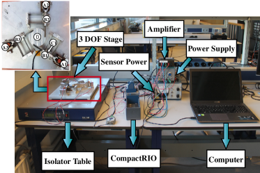
Figure 6: The whole setup including computer, CompactRio, power supply, sensor power, amplifier, isolator, sensor and, stage

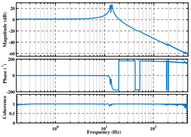
Figure 7: FRF measurement of considered SISO position of the Spyder stage

In [38] a non-linear phase compensator, which is termed “Constant in gain Lead in phase” (CgLp) (for more detail see [35, 16, 38]), has been used to improve the performance of this precision positioning stage. CgLp compensators, consisting of a first/second order lead filter and a GFORE/GSORE, have been utilized along with a PID controller to enhance the precision of the system. In the following, stability properties of two CgLp+PID controllers, one of which has GSORE and the other has SOSRE, are assessed with the proposed methods. The general structure of the controller is

$$C(s) {=} K_{p}\underbrace{\overbrace{\left(\cancelto{A_{\rho}}{\dfrac{1}{s^{2}+2\xi\omega_{r}s+\omega_{r}^{2}}}\right)}^{\text{GSORE}}\overbrace{\left(\dfrac{s^{2}+2\xi_{d}\omega_{d}s+\omega_{d}^{2}}{s^{2}+20\omega_{c}+100\omega_{c}^{2}}\right)}^{\text{Lead}}}_{\text{CgLp}}$$ (66)

$${\times}\underbrace{\overbrace{\left(1+\frac{\omega_{c}}{10s}\right)}^{\text{PI}}\overbrace{\left(\dfrac{\frac{3s}{\omega_{c}}+1}{\frac{s}{3\omega_{c}}+1}\right)}^{\text{Lead}}}_{\text{PID}},$$

in which $\omega_{c}$ is the cross-over frequency and $K_{p}$, $\gamma$, $\omega_{d}$, $\omega_{r}$, $\xi$, and $\xi_{d}$ are tuning parameters. The PID part is tuned on the basis of [39, 18] and the CgLp part is tuned on the basis of [38, 29, 31], and $K_{p}$ is set so that $\omega_{c}=200\pi$, considering the Describing Function (DF) method [38]. In addition, no shaping filter is used for modifying the performance of the reset controller (i.e. $\mathcal{C}_{s}(s)=1$). Note that the tuning of the CgLp compensator is not within the scope of this paper, and we only discuss how to assess stability properties of reset control systems with these compensators.

Remark 5.1.

Suppose that the $H_{\beta}$ condition is/is not satisfied for the reset control system (8) with $\mathcal{C}_{s}(s)$, $C_{L_{1}}(s)$, $C_{L_{2}}(s)$, $C_{R}(s)$, $G(s)$, and $A_{\rho}$. Then the $H_{\beta}$ condition is/is not satisfied for the reset control system (8) with $\mathcal{C}_{s}(s)$, $C^{\prime}_{L_{1}}(s)$, $C^{\prime}_{L_{2}}(s)$, $C_{R}(s)$, $G^{\prime}(s)$, and $A_{\rho}$ if $C^{\prime}_{L_{1}}(s)C^{\prime}_{L_{2}}(s)G^{\prime}(s)=C_{L_{1}}(s)C_{L_{2}}(s)G(s)$ and $G^{\prime}(s)$ is strictly proper. In other words, the “position” of the reset element does not change in the $H_{\beta}$ condition. However, the “position” of the reset element has effects on the performance of the reset control systems [14]. In the two following examples, the sequence of control filters is such that the tracking error is the input of the reset element and other linear parts following in series.

5.1 A Reset control system with GSORE

In the case of GSORE, the control parameters are $\gamma_{1}=\gamma_{2}=0.5$, $\omega_{r}=800\pi$, $\omega_{d}=720\pi$, $K_{p}=8.5273e^{7}$, and $\xi=\xi_{d}=1$. Since the controller has a pole at the origin, we use Definition 4.2 to assess stability properties of this reset control system. Using Proposition 2 yields $340<\dfrac{Q_{2}}{Q_{1}}<5057$ and $1132<\dfrac{Q_{3}}{Q_{4}}$ for $\mathcal{S}_{1}$ and $\mathcal{S}_{2}$, respectively. Thus, we have to solve the optimization problem $M=\underset{Q_{1},Q_{2},Q_{3},Q_{4}}{\min}\ G_{1}(Q_{1},Q_{2},Q_{3},Q_{4})$ such that the following constraints hold

This optimization problem is solved using Genetic Algorithm and Proposition 2. The optimal solution is $Q_{1}=13172$, $Q_{2}=12001144$, $Q_{3}=8113151$, and $Q_{4}=1055$, yielding $M=3.5$ (note that it is not necessary to find the global minimum in these methods). Furthermore, $(\bar{A},C_{0})$ is observable and $(\bar{A},B_{0})$ is controllable. Hence, the reset control system is of Type III and using Theorem 3 this GSORE has the UBIBS property for $A_{\rho}=\gamma I,\ -1<\gamma<1$. Furthermore, since $\dfrac{Q_{1}Q_{3}}{Q_{2}Q_{4}}>\Gamma(-0.5,0.5)$ and $\dfrac{Q_{1}Q_{3}}{Q_{2}Q_{4}}>\Gamma(0.5,-0.5)$, Theorem 3 holds for the considered closed-loop system with $A_{\rho}=\begin{bmatrix}0.5&0\\ 0&-0.5\end{bmatrix}$ or $A_{\rho}=\begin{bmatrix}-0.5&0\\ 0&0.5\end{bmatrix}$. In Fig. 8 the step responses of the closed-loop Spider stage (Fig. 6) with the designed controller for different values of $\gamma_{i}$ are displayed. As it can be observed, the values of $\gamma_{i}$ have effect on the performance of the system. In the sense of transient response, the reset controller with $\gamma_{1}=\gamma_{2}=0.5$ has better performance among other configurations (for more detail see [38, 29]).

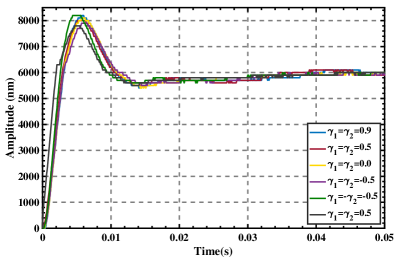
Figure 8: Step response of the closed-loop system with the designed GSORE for different values of $\gamma_{i}$

5.2 Reset control system with SOSRE

In the case in which the controller is a SOSRE the control parameters are $-1<\gamma<1$, $\omega_{r}=150\pi$, $\omega_{d}=96\pi$, $K_{p}=1.135e^{6}$, and $\xi=\xi_{d}=1$. Since the controller has a pole at the origin, we use Definition 3 with the NSV defined in Corollary 4.7 to assess stability properties. The phase of the NSV for this example is shown in Fig. 9. Since the phase of the NSV for this example is between $(-\dfrac{\pi}{2},\pi)$ and the difference between its maximum and its minimum is less than $\pi$, by Remark 2 the reset control system is of Type I. Moreover, the time regularization technique (to prevent successive reset instants, i.e. if the reset happened at one sample time before, the system does not reset) is used to guarantee the well-posedness property. Consequently, by Corollary 4.7 the designed SOSRE yields a closed-loop system which has the UBIBS property. The step responses of the closed-loop Spider stage (Fig. 6) with the designed controller for different values of $\gamma$ are shown in Fig. 10. In the sense of transient response, reset control system with $\gamma=0.5$ has better performance among other controllers. For deeper insights on the performance of closed-loop reset control systems with SOSRE see [31, 29].

Figure 9: $\phase{\vec{\mathcal{N}}(\omega)}$ for the reset control systems with SOSORE

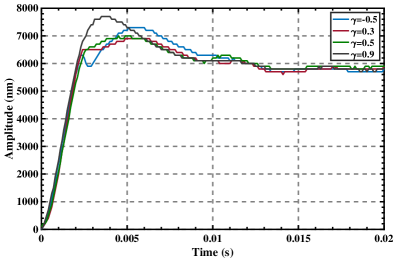
Figure 10: Step response of the closed-loop system with the designed SOSRE for different values of $\gamma$

6 Conclusion

In this paper a novel frequency-domain approach based on the $H_{\beta}$ condition for assessing stability properties of reset control systems has been proposed. This method can be used to determine stability properties of control systems with first and second order reset elements using FRF measurements of their base linear open-loop system. Consequently, the methods do not need an accurate parametric model of the system and the solution of LMIs. In addition, these methods are applicable to the case in which partial reset techniques are used. The effectiveness of the proposed methods have been illustrated with a practical example. This work has been partially supported by NWO through OTP TTW project $\#$16335, by the EACEA, by the European Union’s Horizon 2020 Research and Innovation Programme under grant agreement No 739551 (KIOS CoE), and by the Italian Ministry for Research in the framework of the 2017 Program for Research Projects of National Interest (PRIN), Grant no. 2017YKXYXJ.

Appendix A Proof of Lemma 1

It has been shown in [12] that when $A_{\rho}=0$, $\mathcal{C}_{s}(s)=1$, Assumption 2 holds, and the $H_{\beta}$ condition is satisfied, the reset control system has the UBIBS property. In what follows, we provide a slight modification of the proof in [12] to deal with the case $A_{\rho}\neq 0$. The base linear dynamic of the reset control system is given by

$$\begin{cases}\dot{x}_{l}(t)=\bar{A}x_{l}(t)+\bar{B}w(t),\\ y_{l}(t)=\bar{C}x_{l}(t),\end{cases}$$ (68)

where $x_{l}(t)=[x_{r_{l}}(t)^{T}\ \zeta_{l}(t)^{T}]^{T}\in\mathbb{R}^{n_{p}+n_{r}}$. Denoting $z(t):x(t)-x_{l}(t)=[z_{p}(t)^{T}\ \ z_{r}(t)^{T}]^{T}$, yields

$$\begin{cases}\dot{z}(t)=\bar{A}z(t),&e(t)\neq 0,\\ z(t^{+})=\bar{A}_{\rho}z(t)+(\bar{A}_{\rho}-I)x_{l}(t),&e(t)=0.\\ \end{cases}$$ (69)

According to [12], it is sufficient to show that $z(t)$ is bounded. Since the $H_{\beta}$ condition is satisfied, there exists a matrix $P=P^{T}>0$ such that

$$P=\begin{bmatrix}P_{1}&(\beta\bar{C}_{e})^{T}\\ \beta\bar{C}_{e}&\Varrho\end{bmatrix},\ P_{1}=P_{1}^{T}>0.$$ (70)

Consider now the quadratic Lyapunov function $V(t)=z(t)^{T}Pz(t)$. Using the same procedure as in [12] yields

$$V(t)\leq e^{-\epsilon(t-t_{i})}V(t_{i}),\quad t\in(t_{i},t_{i+1}],\ \epsilon>0,$$ (71)

and

$$V(t_{i}^{+}) {=} V(t_{i})+x_{r}^{T}(t_{i})(A_{\rho}^{T}\Varrho A_{\rho}-\Varrho)x_{r}(t_{i})$$

$${+}\>2(A_{\rho}^{T}-I)x_{r}^{T}(t_{i})\beta\bar{C}_{e}z_{p}(t_{i})-2x^{T}_{r}(t_{i})A_{\rho}^{T}\Varrho x_{r_{l}}(t_{i}),$$

in which $t_{i}$ are the reset instants. Now, let the maximum eigenvalue of $A_{\rho}^{T}\Varrho A_{\rho}-\Varrho$ be $\lambda_{\max}$ and note that $\lambda_{\max}<0$ since $A_{\rho}^{T}\Varrho A_{\rho}-\Varrho<0$. As a result

$$V(t_{i}^{+}) {\leq} V(t_{i})-|\lambda_{\max}|x_{r}^{T}(t_{i})x_{r}(t_{i})+2(A_{\rho}^{T}-I)x_{r}^{T}(t_{i})\beta\bar{C}_{e}z_{p}(t_{i})$$

$${-}\>2x^{T}_{r}(t_{i})A_{\rho}^{T}\Varrho x_{r_{l}}(t_{i})\Rightarrow$$

$$V(t_{i}^{+}) {\leq} V(t_{i})+2\left\lVert x_{r}(t_{i})\right\rVert(||A_{\rho}^{T}-I||\left\lVert\beta\bar{C}_{e}z_{p}(t_{i})\right\rVert$$ (73)

$${+}\>||A_{\rho}\Varrho x_{r_{l}}(t_{i})||).$$

At the reset instants $|\bar{C}_{e}z_{p}(t_{i})|\leq|D_{e}r(t)|$ which implies that $|\bar{C}_{e}z_{p}(t_{i})|$ is bounded. Moreover, since the base linear system is stable, $x_{r_{l}}(t_{i})$ is bounded. Assume now that $x_{r}(t_{i})$ is unbounded. By (71) and (A), we conclude that $\displaystyle\lim_{i\to\infty}V(t_{i})=0$. This is a contradiction because $z(t)=0\Rightarrow x(t)=x_{l}(t)$ which implies that the system is a stable linear system with bounded state. Therefore, $x_{r}(t_{i})$ is bounded. Now, we prove that $\dot{x}_{r}(t_{i})$ is bounded. If reset happens when the input of the reset element is zero (i.e. $\mathcal{C}_{s}(s)=1$) and Assumption 2 holds, then

$$\dfrac{dx_{r}(t)}{dt}\Big{|}_{t=t_{i}^{-}} {=} A_{r}\left(e^{A_{r}(t_{i}-t_{i-1})}x_{r}(t_{i-1})+\displaystyle\int_{t_{i-1}}^{t_{i}}e^{A_{r}(t_{i}-\tau)}B_{r}e(\tau)d\tau\right)$$

$${=} A_{r}x_{r}(t_{i})\Rightarrow\left\lvert\dot{x}_{r}(t_{i}^{-})\right\rvert=\left\lvert A_{r}x_{r}(t_{i})\right\rvert.$$

Thus, since $|x_{r}(t_{i})|$ is bounded, $\left\lvert\dot{x}_{r}(t_{i}^{-})\right\rvert$ is bounded. As a result, since $|x_{r}(t_{i-1}^{+})|\leq|A_{\rho}||x_{r}(t_{i-1})|$, $|x_{r}(t_{i})|$ and $\left\lvert\dot{x}_{r}(t_{i}^{-})\right\rvert$ are bounded,

$$\exists\ K_{1}>0,\ \alpha>0\ \text{such that }|x_{r}(t_{i})|\leq K_{1}\left(1-e^{\alpha(t_{i}-t_{i-1})}\right),\ \forall\ t_{i}.$$ (75)

Now assume that there exist $t_{i}$ and $t_{i-1}$ such that for any $\epsilon>0$, $t_{i}-t_{i-1}<\epsilon$. Thus, by (75) and for sufficient small $\epsilon$, $x_{r}(t_{i})\to 0$. This is a contradiction because $(I-\bar{A}_{\rho})x_{r}(t_{i})\to 0$ which means that $t_{i}$ is not a reset instant. Thus, there exists $\lambda>0$ such that, for all $k\in\mathbb{N}$, $\lambda\leq t_{k+1}-t_{k}$. Therefore, the reset instants have the the well-posedness property (see Definition 1).
In the case in which $\mathcal{C}_{s}=1$ or Assumption 2 does not hold, (74) can not be concluded. However, if the well-posedness property of the reset instants holds, then there exists $\lambda>0$ such that, for all $k\in\mathbb{N}$, $\lambda\leq t_{k+1}-t_{k}$. In addition, since $|x_{r}(t_{i-1}^{+})|\leq|A_{\rho}||x_{r}(t_{i-1})|$ and $|x_{r}(t_{i})|$ are bounded, we conclude (75). Since the system has the well-posedness property, the reset control system (8) has an unique well-defined solution for any initial condition $x_{0}$ and any input $w$ which is a Bohl function [7]. The rest of the proof is the same as the proof in [12].

Appendix B Proof of Corollary 3.2

Let $\beta^{\prime}=-\beta$ and $\Varrho^{\prime}=\dfrac{\Varrho}{C_{r}}$. By the proof of the $H_{\beta}$ condition in [12] the transfer function (10) for the configuration shown in Fig. 4) can be rewritten as (see also Fig. 11)

$$H(s)=\dfrac{\beta^{\prime}\dfrac{L^{\prime}(s)}{\mathcal{C}_{s}(s)}+\Varrho^{\prime}C_{R}(s)}{1+L^{\prime}(s)}.$$ (76)

Let $C_{L_{1}}(s)C_{L_{2}}(s)C_{R}(s)G(s)=\dfrac{k_{m}s^{m}+k_{m-1}s^{m-1}+...+k_{0}}{s^{n}+k^{\prime}_{n-1}s^{n-1}+...+k^{\prime}_{0}}$. Using the NSV defined in (4.1), one could repeat Steps 1 to 4 of the proof of Theorem 1. Note that $K_{s_{0}}\beta^{\prime}$ in (20)-(24) and (28) has to be replaced by $\dfrac{\beta^{\prime}}{K_{s_{0}}}$ and $K_{n}$ has also to be replaced by $k_{n}$ in (25).

Figure 11: The block diagram of $H_{\beta}$ condition for the modified architecture Fig. 4 with GFORE or PCI

Appendix C Proof of Proposition 2

Consider $Q_{1}\mathcal{F}_{1}(\omega)+Q_{2}\mathcal{F}_{2}(\omega)$ as the scalar product of the two vectors $\vv{\mathcal{F}}(\omega)$ and $\vv{\mathcal{Q}}$. Thus, for all $\omega\in\mathbb{R}^{+}$, the condition (33) can be re-written as

$$\sqrt{Q_{1}^{2}+Q_{2}^{2}}\sqrt{\mathcal{F}_{1}^{2}(\omega)+\mathcal{F}_{2}^{2}(\omega)}\cos(\vartheta)>\mathcal{F}_{3}(\omega).$$ (77)

As a result, when $\mathcal{F}_{3}(\omega)\geq 0$, $\cos(\vartheta)$ must be positive and

$$\sqrt{Q_{1}^{2}+Q_{2}^{2}}>\underset{\omega\in\omega_{p}}{\max\ }\dfrac{\mathcal{F}_{3}(\omega)}{\cos(\vartheta)\sqrt{\mathcal{F}^{2}_{1}(\omega)+\mathcal{F}^{2}_{2}(\omega)}}=\eta_{1}(\dfrac{Q_{2}}{Q_{1}}).$$ (78)

Positivity of $\cos(\vartheta)$ implies $\dfrac{Q_{2}}{Q_{1}}\in g_{p}$. When $\mathcal{F}_{3}(\omega)<0$, there are two solutions for condition (77). $\cos(\vartheta)\geq 0$ which requiers $\dfrac{Q_{2}}{Q_{1}}\in g_{N}$, or

$$\sqrt{Q_{1}^{2}+Q_{2}^{2}}<\underset{\omega\in\omega_{N}}{\min\ }\dfrac{\mathcal{F}_{3}(\omega)}{\cos(\vartheta)\sqrt{\mathcal{F}^{2}_{1}(\omega)+\mathcal{F}^{2}_{2}(\omega)}}=\eta_{2}(\dfrac{Q_{2}}{Q_{1}}).$$ (79)

Therefore, by (78) and (79) $\eta_{2}(\dfrac{Q_{2}}{Q_{1}})>\eta_{1}(\dfrac{Q_{2}}{Q_{1}})$ and the proof is complete.

Appendix D Proof of Corollary 4.6

First, a preliminary result is stated and proved.

Lemma D.1.

Consider the reset controllers $C_{R_{1}}$ and $C_{R_{2}}$ shown in Fig. 12. Suppose $C_{R_{1}}$ and $C_{R_{2}}$ have the same base linear system, are strictly proper, and have different state-space realizations. Then if $A_{\rho}=\gamma I$ and their initial conditions are zero, $y_{1}(t)=y_{2}(t)$, for $t\geq 0$.

Figure 12: Two reset controllers $C_{R_{1}}$ and $C_{R_{2}}$ with different realizations

Let $A_{r_{1}}$, $B_{r_{1}}$, and $C_{r_{1}}$ be the state-space realization of $C_{R_{1}}(s)$ and $A_{r_{2}}$, $B_{r_{2}}$, and $C_{r_{2}}$ be the state-space realization of $C_{R_{2}}(s)$. Since the base transfer function of $C_{R_{1}}(s)$ and $C_{R_{2}}(s)$ are the same,

$$C_{r_{1}}\displaystyle\int_{t_{0}}^{t}e^{A_{r_{1}}(t-\tau)}B_{r_{1}}u(\tau)d\tau=C_{r_{2}}\displaystyle\int_{t_{0}}^{t}e^{A_{r_{2}}(t-\tau)}B_{r_{2}}u(\tau)d\tau.$$ (80)

Let $t_{k},\ k\in\mathbb{N}$, be the reset instants of $C_{R_{1}}$ and $C_{R_{2}}$. Since the initial condition is zero,

$$y_{1}(t) {=} C_{r_{1}}\Big{(}\displaystyle\int_{t_{k}}^{t}e^{A_{r_{1}}(t-\tau)}B_{r_{1}}u(\tau)d\tau+\gamma\displaystyle\int_{t_{k-1}}^{t_{k}}e^{A_{r_{1}}(t-\tau)}B_{r_{1}}u(\tau)d\tau$$

$${+}\>\cdots+\gamma^{k}\displaystyle\int_{t_{0}}^{t_{1}}e^{A_{r_{1}}(t-\tau)}B_{r_{1}}u(\tau)d\tau\Big{)},$$

$$y_{2}(t) {=} C_{r_{2}}\Big{(}\displaystyle\int_{t_{k}}^{t}e^{A_{r_{2}}(t-\tau)}B_{r_{2}}u(\tau)d\tau+\gamma\displaystyle\int_{t_{k-1}}^{t_{k}}e^{A_{r_{2}}(t-\tau)}B_{r_{2}}u(\tau)d\tau$$

$${+}\>\cdots+\gamma^{k}\displaystyle\int_{t_{0}}^{t_{1}}e^{A_{r_{2}}(t-\tau)}B_{r_{2}}u(\tau)d\tau\Big{)}.$$

As a result, $y_{1}(t)=y_{2}(t)$, for all $t\geq 0$ by (80). The corollary is now proved. Using Lemma D.1, since the initial condition of the reset part are zero and $A_{\rho}=\gamma I$, the states $\zeta(t)$ are the same for different state-space realizations of $C_{R}(s)$ of the reset control system (8). Thus, since Theorem 3 holds for the reset control system (8) with GSORE (5) with the controllable realization (6), $\zeta(t)$, which contains $u_{1}(t)$ and $u_{r}(t)$, is also bounded in the reset control system (8) with GSORE (5) with realization configurations (61) and (62). Therefore, it is just needed to show that the reset state $x_{r}(t)$ is bounded. Consider the reset controller (1). Now assume that $x_{r}(t)$ is unbounded, since $u_{1}(t)$ is bounded and by state-space realization (61) and (62), $u_{r}(t)$ becomes unbounded which is a contradiction. Therefore, $x_{r}(t)$ must be bounded and the proof is complete.

References

• [1] A. A. Dastjerdi, A. Astolfi, and S. H. HosseinNia. A frequency-domain stability method for reset systems. In IEEE 59th Conference on Decision and Control, 2020.
• [2] W. H. T. M. Aangenent, G. Witvoet, W. P. M. H. Heemels, M. J. G. van de Molengraft, and M. Steinbuch. Performance analysis of reset control systems. International Journal of Robust and Nonlinear Control, 20(11):1213–1233, 2010.
• [3] Alfonso Baños and Antonio Barreiro. Reset control systems. Springer Science $\&$ Business Media, 2011.
• [4] Alfonso Banos, Joaquin Carrasco, and Antonio Barreiro. Reset times-dependent stability of reset control with unstable base systems. In 2007 IEEE International Symposium on Industrial Electronics, pages 163–168. IEEE, 2007.
• [5] Alfonso Baños, Joaquín Carrasco, and Antonio Barreiro. Reset times-dependent stability of reset control systems. IEEE Transactions on Automatic Control, 56(1):217–223, 2010.
• [6] Alfonso Baños and Miguel A Davó. Tuning of reset proportional integral compensators with a variable reset ratio and reset band. IET Control Theory & Applications, 8(17):1949–1962, 2014.
• [7] Alfonso Banos, Juan I Mulero, Antonio Barreiro, and Miguel A Davo. An impulsive dynamical systems framework for reset control systems. International Journal of Control, 89(10):1985–2007, 2016.
• [8] Antonio Barreiro, Alfonso Baños, Sebastián Dormido, and José A González-Prieto. Reset control systems with reset band: Well-posedness, limit cycles and stability analysis. Systems & Control Letters, 63:1–11, 2014.
• [9] R. Beerens, A. Bisoffi, L. Zaccarian, W.P.M.H. Heemels, H. Nijmeijer, and N. van de Wouw. Reset integral control for improved settling of pid-based motion systems with friction. Automatica, 107:483 – 492, 2019.
• [10] R. Beerens, A. Bisoffi, L. Zaccarian, W.P.M.H. Heemels, H. Nijmeijer, and N. van de Wouw. Reset integral control for improved settling of pid-based motion systems with friction. Automatica, 107:483 – 492, 2019.
• [11] O Beker, CV Hollot, Q Chen, and Y Chait. Stability of a reset control system under constant inputs. In Proceedings of the 1999 American Control Conference (Cat. No. 99CH36251), volume 5, pages 3044–3045. IEEE, 1999.
• [12] Orhan Beker, C.V. Hollot, Y. Chait, and H. Han. Fundamental properties of reset control systems. Automatica, 40(6):905 – 915, 2004.
• [13] A. Bisoffi, R. Beerens, W.P.M.H. Heemels, H. Nijmeijer, N. van de Wouw, and L. Zaccarian. To stick or to slip: A reset pid control perspective on positioning systems with friction. Annual Reviews in Control, 49:37 – 63, 2020.
• [14] Chengwei Cai, Ali Ahmadi Dastjerdi, Niranjan Saikumar, and S.H. HosseinNia. The optimal sequence for reset controllers. In $18^{th}$ European Control Conference (ECC 2020), 2020.
• [15] Joaquín Carrasco, Alfonso Baños, and Arjan van der Schaft. A passivity-based approach to reset control systems stability. Systems & Control Letters, 59(1):18–24, 2010.
• [16] L. Chen, N. Saikumar, and S. H. HosseinNia. Development of robust fractional-order reset control. IEEE Transactions on Control Systems Technology, 28(4):1404–1417, 2020.
• [17] J. C. Clegg. A nonlinear integrator for servomechanisms. Transactions of the American Institute of Electrical Engineers, Part II: Applications and Industry, 77(1):41–42, 1958.
• [18] Ali Ahmadi Dastjerdi, Niranjan Saikumar, and S. Hassan HosseinNia. Tuning guidelines for fractional order PID controllers: Rules of thumb. Mechatronics, 56:26 – 36, 2018.
• [19] Fulvio Forni, Dragan Nešić, and Luca Zaccarian. Reset passivation of nonlinear controllers via a suitable time-regular reset map. Automatica, 47(9):2099 – 2106, 2011.
• [20] Wynita M Griggs, Brian DO Anderson, Alexander Lanzon, and Michael C Rotkowitz. A stability result for interconnections of nonlinear systems with “mixed” small gain and passivity properties. In 2007 46th IEEE Conference on Decision and Control, pages 4489–4494. IEEE, 2007.
• [21] Yuqian Guo, Youyi Wang, and Lihua Xie. Frequency-domain properties of reset systems with application in hard-disk-drive systems. IEEE Transactions on Control Systems Technology, 17(6):1446–1453, 2009.
• [22] Yuqian Guo, Lihua Xie, and Youyi Wang. Analysis and Design of Reset Control Systems. Institution of Engineering and Technology, 2015.
• [23] L. Hazeleger, M. Heertjes, and H. Nijmeijer. Second-order reset elements for stage control design. In American Control Conference (ACC), pages 2643–2648, 2016.
• [24] M.F. Heertjes, K.G.J. Gruntjens, S.J.L.M. van Loon, N. Kontaras, and W.P.M.H. Heemels. Design of a variable gain integrator with reset. In American Control Conference (ACC), Chicago, USA, pages 2155–2160, 2015.
• [25] CV Hollot, Orhan Beker, Yossi Chait, and Qian Chen. On establishing classic performance measures for reset control systems. In Perspectives in robust control, pages 123–147. Springer, 2001.
• [26] CV Hollot, Y Zheng, and Y Chait. Stability analysis for control systems with reset integrators. In Proceedings of the 36th IEEE Conference on Decision and Control, volume 2, pages 1717–1719. IEEE, 1997.
• [27] Isaac Horowitz and Patrick Rosenbaum. Non-linear design for cost of feedback reduction in systems with large parameter uncertainty. International Journal of Control, 21(6):977–1001, 1975.
• [28] S Hassan HosseinNia, Inés Tejado, and Blas M Vinagre. Fractional-order reset control: Application to a servomotor. Mechatronics, 23(7):781–788, 2013.
• [29] Nima Karbasizadeh, Ali Ahmadi Dastjerdi, Niranjan Saikumar, Duarte Valerio, and S.H. HosseinNia. Benefiting from linear behaviour of a nonlinear reset-based element at certain frequencies. In Australian and New Zealand Control Conference (ANZCC), 2020.
• [30] Nima Karbasizadeh, Ali Ahmadi Dastjerdi, Niranjan Saikumar, and S Hassan HosseinNia. and-passing nonlinearity in reset elements. arXiv preprint arXiv:2005.02887, 2020.
• [31] Nima Karbasizadeh, Niranjan Saikumar, and S Hassan Hoseinnia. Fractional-order single state reset element. Nonliner Dynamics, 2021.
• [32] Hassan K Khalil and Jessy W Grizzle. Nonlinear systems, volume 3. Prentice hall Upper Saddle River, NJ, 2002.
• [33] Dragan Nešić, Luca Zaccarian, and Andrew R Teel. Stability properties of reset systems. Automatica, 44(8):2019–2026, 2008.
• [34] D Paesa, J Carrasco, O Lucia, and C Sagues. On the design of reset systems with unstable base: A fixed reset-time approach. In IECON 2011-37th Annual Conference of the IEEE Industrial Electronics Society, pages 646–651. IEEE, 2011.
• [35] A. Palanikumar, N. Saikumar, and S. H. HosseinNia. No more differentiator in PID: Development of nonlinear lead for precision mechatronics. In European Control Conference (ECC), pages 991–996, 2018.
• [36] Svetlana Polenkova, Jan W Polderman, and Romanus Langerak. Stability of reset systems. In Proceedings of the 20th International Symposium on Mathematical Theory of Networks and Systems, pages 9–13, 2012.
• [37] KE Rifai and J-JE Slotine. Compositional contraction analysis of resetting hybrid systems. IEEE Transactions on Automatic Control, 51(9):1536–1541, 2006.
• [38] N. Saikumar, R. K. Sinha, and S. H. HosseinNia. ‘Constant in gain Lead in phase’ element-application in precision motion control. IEEE/ASME Transactions on Mechatronics, 24(3):1176–1185, 2019.
• [39] R Munnig Schmidt, Georg Schitter, and Adrian Rankers. The Design of High Performance Mechatronics High-Tech Functionality by Multidisciplinary System Integration. IOS Press, 2014.
• [40] Duarte Valério, Niranjan Saikumar, Ali Ahmadi Dastjerdi, Nima Karbasizadeh, and S Hassan HosseinNia. Reset control approximates complex order transfer functions. Nonlinear Dynamics, pages 1–15, 2019.
• [41] S. J. A. M. Van den Eijnden, Y. Knops, and M. F. Heertjes. A hybrid integrator-gain based low-pass filter for nonlinear motion control. In IEEE Conference on Control Technology and Applications (CCTA), pages 1108–1113, 2018.
• [42] S.J.L.M. van Loon, K.G.J. Gruntjens, M.F. Heertjes, N. van de Wouw, and W.P.M.H. Heemels. Frequency-domain tools for stability analysis of reset control systems. Automatica, 82:101 – 108, 2017.
• [43] Paolo Vettori, Jan Willem Polderman, and Rom Langerak. A geometric approach to stability of linear reset systems. Proceedings of the 21st Mathematical Theory of Networks and Systems, 2014.
• [44] A. F. Villaverde, A. B. Blas, J. Carrasco, and A. B. Torrico. Reset control for passive bilateral teleoperation. IEEE Transactions on Industrial Electronics, 58(7):3037–3045, 2011.
• [45] L. Zaccarian, D. Nesic, and A. R. Teel. First order reset elements and the Clegg integrator revisited. In American Control Conference, pages 563–568 vol. 1, 2005.
• [46] Jinchuan Zheng, Yuqian Guo, Minyue Fu, Youyi Wang, and Lihua Xie. Improved reset control design for a pzt positioning stage. In 2007 IEEE International Conference on Control Applications, pages 1272–1277. IEEE, 2007.