Performance-Agnostic Fusion of Probabilistic Classifier Outputs
^*

Abstract

We propose a method for combining probabilistic outputs of classifiers to make a single consensus class prediction when no further information about the individual classifiers is available, beyond that they have been trained for the same task. The lack of relevant prior information rules out typical applications of Bayesian or Dempster-Shafer methods, and the default approach here would be methods based on the principle of indifference, such as the sum or product rule, which essentially weight all classifiers equally. In contrast, our approach considers the diversity between the outputs of the various classifiers, iteratively updating predictions based on their correspondence with other predictions until the predictions converge to a consensus decision. The intuition behind this approach is that classifiers trained for the same task should typically exhibit regularities in their outputs on a new task; the predictions of classifiers which differ significantly from those of others are thus given less credence using our approach. The approach implicitly assumes a symmetric loss function, in that the relative cost of various prediction errors are not taken into account. Performance of the model is demonstrated on different benchmark datasets. Our proposed method works well in situations where accuracy is the performance metric; however, it does not output calibrated probabilities, so it is not suitable in situations where such probabilities are required for further processing.

I Introduction

In classifying an observation, the members of an ensemble of (probabilistic) classifiers will typically disagree, with individual classifiers sometimes producing markedly different predictions for the same observation. Leveraging such disagreement can be the very basis of improved overall performance, for example in boosting, where different subsets of classifiers might perform better in different settings [1]. Similar predictions are typically easy to handle when a single class prediction must be made; however, it is trickier to reach consensus decisions for markedly different predictions [2].

We consider the problem of fusing probabilistic classifier predictions to reach a consensus decision, i.e. a decision all members agree to support in the best interest of the whole group [3]. The key assumption we make is that the various classifiers have been trained to perform the same classification task. As a result, we would expect the classifier outputs to be quite similar, particularly in regions where they have fairly high confidence. In regions where a classifier is not confident about class probabilities, it is more likely that its prediction deviates more notably from those of other classifiers.

Various approaches have been developed [4] to take advantage of diverse classifier performance in different settings, including Bayesian methods [5] and Dempster-Shafer (DS) methods [6]. However, these approaches invariably make use of information about prior performance of the classifiers, such as the training or test error. Such information about classifier performance is invaluable for high-performance classifier fusion, since it allows one to account explicitly for the quality of each classifier. For DS methods, for instance, such information is used to form basic probability assignments of all subsets of classes [6]. This paper considers the challenging situation where the classifiers are particularly opaque, more so than in the traditional black-box setting: we do not know what model each classifier uses, how or on what data the classifier was trained, what features it was trained with, its performance on any past data, or any of its predictions on any previous observations.

In this setting, the most natural approach would be to use the principle of indifference [7], treating all of the classifiers equally. Prominent approaches based on this principle are the sum rule, the product rule, the majority vote rule [8] and the Borda count rule [9]. The approach we present here relies on the assumption that simply because various classifiers were trained for the same task, we expect there to be regularities in their outputs on future observations, which we should be able to leverage to obtain improved fused decisions relative to approaches using the principle of indifference.

This work is inspired by the negotiation process, where stakeholders (classifiers) attempt to reach consensus decisions: stakeholders gradually update their position during the negotiations until consensus is reached. Our approach is similarly an iterative process, in which initial classifier outputs are transformed to become more similar with the aim of reaching consensus.

Contributions

This paper introduces a classifier fusion method which takes advantage of prediction similarities to enhance consensus decision-making in once-off classifier fusion. While classifiers are not ultimately weighted equally, the approach is rooted in the principle of indifference, in that no external information is used to weight their relative importance. Rather, the fusion mechanism used leverages discrepancies between the predictions of the various classifiers on the observation of interest: fusion is essentially achieved by updating a probability vector for each classifier—initialized with the initial predictions—based on the discrepancies between them until they agree.

We empirically evaluate our proposed approach on a number of benchmark datasets from the UCI machine learning repository[10], as well as one from the Columbia object image library[11]. We observe that the accuracy of our approach generally exceeds those of the sum, product, majority vote, and Borda count rules in a variety of settings.

II Background and Literature Review

While there is a vast literature on classifier fusion, the “zero-knowledge” situation we consider in this paper has received relatively little attention. In general, the lack of knowledge about the various classifiers would lead one to consider approaches based on the principle of indifference. Kittler et al. analyse and empirically compare various fusion approaches based on this principle, and note that the sum rule exhibited the best performance [8]. They attribute this to its lower sensitivity to estimation errors in individual classifier outputs.

We next introduce the sum rule, product rule, majority vote rule and Borda count rule. We wish to combine $m$ classifiers’ predictions for an $l$-class classification task on a single input observation $x_{\text{in}}$. Specifically, the $j$-th classifier $f_{j}$ outputs a probability vector $d_{j}=f_{j}(x_{\textbf{in}})$ of length $l$.

Sum rule

The fused output using the sum rule is

$$\frac{1}{m}\sum_{j=1}^{m}d_{j}=\frac{1}{m}\bigg{(}\sum_{j=1}^{m}d_{j1},\sum_{j=1}^{m}d_{j2},\cdots,\sum_{j=1}^{m}d_{jl}\bigg{)}\enspace.$$ (1)

Product rule

The fused output using the product rule is

$$\alpha\prod_{j=1}^{m}d_{j}\equiv\alpha\bigg{(}\prod_{j=1}^{m}d_{j1},\prod_{j=1}^{m}d_{j2},\cdots,\prod_{j=1}^{m}d_{jl}\bigg{)}\enspace,$$ (2)

where $\alpha$ denotes a normalisation constant.

Majority vote rule

Let

$$\Delta_{jk}=\begin{cases}1&\text{if }d_{jk}=\max_{s=1}^{l}d_{js}\\ 0&\text{otherwise. }\end{cases}$$

The fused output using the majority vote rule is

$$\frac{1}{m}\bigg{(}\sum_{j=1}^{m}\Delta_{j1},\sum_{j=1}^{m}\Delta_{j2},\cdots,\sum_{j=1}^{m}\Delta_{jl}\bigg{)}\,.$$ (3)

Borda count rule

In the Borda count rule, classifiers rank classes in order of preference by giving each class a number of points corresponding to the number of classes ranked lower. Let

$$\beta_{jk}=l-|\{d_{ji}:d_{ji}>d_{jk}\lor(d_{ji}=d_{jk}\land i<k)\}|\,.$$

The fused output using the Borda count rule is

$$\frac{2}{ml(l+1)}\bigg{(}\sum_{j=1}^{m}\beta_{j1},\sum_{j=1}^{m}\beta_{j2},\cdots,\sum_{j=1}^{m}\beta_{jl}\bigg{)}\,.$$ (4)

In this work, we will compare the performance of fusion methods for consensus decision-making, assuming a symmetric loss function. In this setting, the optimal decision for any fusion approach is to select the class with largest fused output. In the case of ties, we will arbitrarily select the class with minimum index among those with maximal outputs.

III Classifier Fusion Method

Given $x_{\textbf{in}}$, each classifier $f_{i}$’s output $d_{i}$ will serve as an initial distribution $\pi_{i}^{(0)}$. These initial distributions are the input to the fusion algorithm, and they are updated over a number of iterations until consensus (or an iteration limit) is reached. We call the resulting fusion method the Yayambo algorithm.

During each iteration $t$, each current distribution $\pi_{i}^{(t-1)}$ is updated to a new distribution $\pi_{i}^{(t)}$. These updates are performed based on a vector of non-negative weights computed between each pair of current distributions. Each vector component expresses a level of support for one distribution’s prediction for a specific class from another, and is called a class support. Such a vector of class supports is termed a support. We denote the support for $\pi_{i}^{(t-1)}$ from $\pi_{j}^{(t-1)}$ by $\beta_{ji}^{(t)}$. The updated distribution $\pi_{i}^{(t)}$ is then calculated using the supports for $\pi_{i}^{(t-1)}$:

$$\pi_{ik}^{(t)}=\alpha_{i}^{(t)}\pi_{ik}^{(t-1)}\sum_{j\neq i}\beta_{ji,k}^{(t)}\,,$$ (5)

where the subscript $k$ denotes a vector component (one per class), and $\alpha_{i}^{(t)}$ is a normalisation constant. Since the supports will be non-negative (as discussed later), this yields valid probability distributions at each iteration. Consensus occurs when these distributions stabilize: our implementation requires

$$\sum_{i=1}^{m}\|\pi_{i}^{(t)}-\pi_{i}^{(t-1)}\|_{2}<m\varepsilon$$ (6)

(for $\varepsilon=10^{-6}$). On termination, we combine the final distributions using the sum rule—this simply provides a mechanism for resolving potential cases that do not reach consensus by the iteration limit.

We finally discuss how the required supports $\beta_{ji}^{(t)}$ are calculated based on the current distributions $\pi_{j}^{(t-1)}$ and $\pi_{i}^{(t-1)}$. A support is a vector of positive scores that encodes a notion of similarity between two distributions: when two distributions are more similar, they assign stronger support to each other, as reflected by larger class supports. Support of distributions need not to be symmetric. While various support functions could be defined, the function we consider is inspired by Kullback-Leibler divergence [12].

This notion of support is related to the Matthew Effect [13], where group members with similar beliefs about a topic amplify and collect ever-larger support from each other. In the setting of our work here, if we cluster stakeholders (classifiers) into groups whose predictions are similar, the members of each group will assign stronger support to each other, and assign weaker support to members of other groups.

The class support for $\pi_{i}^{(t-1)}$ from $\pi_{j}^{(t-1)}$ with respect to class $c_{k}$ depends principally on two things: first, the probability $\pi_{j}^{(t-1)}$ assigns to class $c_{k}$ (larger values corresponds to higher class supports), and second on the difference between the probabilities that $\pi_{i}^{(t-1)}$ and $\pi_{j}^{(t-1)}$ assign to class $c_{k}$ (larger differences lead to smaller class supports). Specifically, at iteration $t$, the class $k$ support for $\pi_{i}^{(t-1)}$ from $\pi_{j}^{(t-1)}$ is

$$\beta^{(t)}_{ji,k}=\frac{\pi^{(t-1)}_{jk}}{1+D(\pi_{ik}^{(t-1)},\pi_{jk}^{(t-1)})}\,,$$ (7)

where the dissimilarity for the $k$th components of $\pi_{i}^{(t)}$ and $\pi_{j}^{(t)}$ is given by

$$D(\pi_{ik}^{(t)},\pi_{jk}^{(t)})=\pi^{(t)}_{ik}|\log\frac{\pi^{(t)}_{ik}+\varepsilon_{0}}{\pi^{(t)}_{jk}+\varepsilon_{0}}|\,,$$ (8)

and $\varepsilon_{0}=10^{-6}$ is a smoothing term to avoid zero division. Figure 1 plots the class supports and related quantities in terms of the relevant class $k$ probabilities.

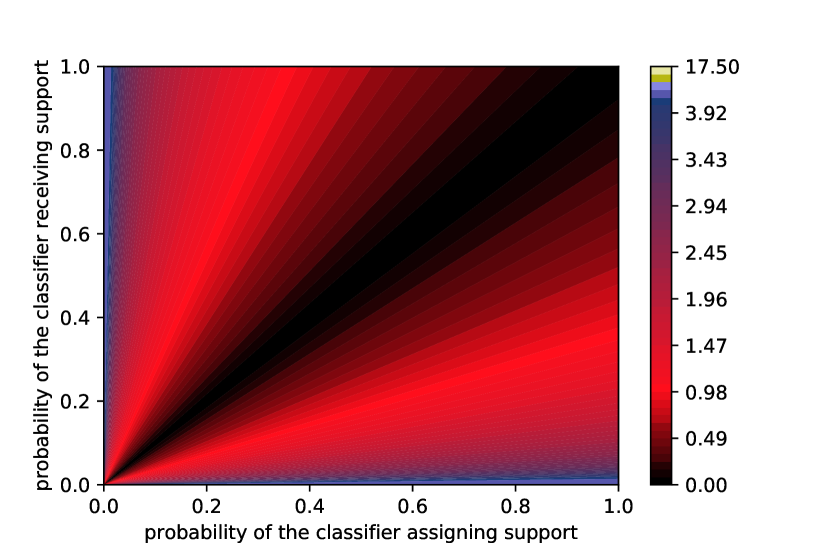
(a)

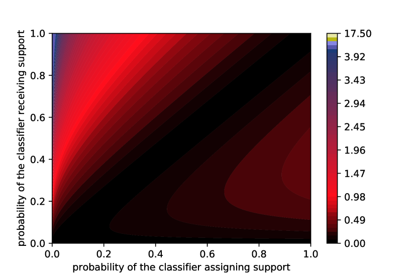
(b)

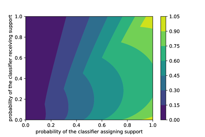
(c)

Figure 1: Various quantities involved in calculation of class supports in Equation 7. (1(a)): The absolute value of the log-ratio defined in the dissimilarity formula (Equation 8). (1(b)): The dissimilarity defined in Equation 8. (1(c)): Class support between probabilities as per Equation 7.

1:  $t\leftarrow 0$

2:  $m\leftarrow\textrm{number of distributions $\pi^{(0)}_{i}$ to fuse}$

3:  repeat

4:     $t\leftarrow t+1$

5:     $\texttt{difference}\leftarrow 0$

6:     for all $i$ do

7:        for all $j\neq i$ do

8:           for all $k=1$ to $l$ do

9:              $\beta^{(t)}_{ji,k}\leftarrow\frac{\pi^{(t-1)}_{jk}}{1+\pi^{(t-1)}_{ik}|\log\frac{\pi^{(t-1)}_{ik}+\varepsilon_{0}}{\pi^{(t-1)}_{jk}+\varepsilon_{0}}|}$

10:           end for

11:        end for

12:        $\pi_{i}^{(t)}\leftarrow(0,0,\cdots,0)$

13:        $\alpha_{i}^{(t)}\leftarrow 0$

14:        for all $j\neq i$ do

15:           for all $k=1$ to $l$ do

16:              $\pi_{ik}^{(t)}\leftarrow\pi_{ik}^{(t)}+\pi_{ik}^{(t-1)}\beta^{(t)}_{ji,k}$

17:              $\alpha_{i}^{(t)}\leftarrow\alpha_{i}^{(t)}+\pi_{ik}^{(t)}$

18:           end for

19:        end for

20:        $\pi^{(t)}_{i}\leftarrow\frac{\pi^{(t)}_{i}}{\alpha_{i}^{(t)}}$

21:        $\texttt{difference}\leftarrow\texttt{difference}+\|\pi_{i}^{(t)}-\pi_{i}^{(t-1)}\|_{2}$

22:     end for

23:  until $\texttt{difference}<m\varepsilon$ or $t==T$

24:  for all $k=1$ to $l$ do

25:     $\varpi_{k}\leftarrow 0$

26:     for all $i$ do

27:        $\varpi_{k}\leftarrow\varpi_{k}+\pi_{ik}^{(t)}$

28:     end for

29:     $\varpi_{k}\leftarrow\frac{\varpi_{k}}{m}$

30:  end for

31:  return  $\varpi$

Algorithm 1 Yayambo(): The algorithm receives as inputs the classifier outputs $\pi_{i}^{(0)}$, a small threshold $\varepsilon_{0}$ to avoid zero division, the convergence threshold $(\varepsilon)$ and the maximum number of iterations $(T)$, and outputs the fusion result $\varpi$.

The resulting algorithm is detailed in Algorithm 1. The source code of Yayambo can be found at https://bitbucket.org/jmf-mas/codes/src/master/classifier. Assuming that $T$ is the number of iterations until termination, its complexity is $\mathcal{O}(Tm^{2}l)$. In terms of computational cost, the Yayambo method is more costly than the benchmark fusion methods. However, for typical $m$ and $T$, this complexity is hardly noticeable. Table I illustrates the algorithm, showing the evolution of two distributions $\pi_{1}^{(t)}$ and $\pi_{2}^{(t)}$ during execution. In this example, convergence is reached after 7 iterations.

$t$	$\pi_{1}^{(t)}$	$\pi_{2}^{(t)}$	$\pi^{(t)}$	$\sum_{i=1}^{2}\|\pi_{i}^{(t)}-\pi_{i}^{(t-1)}\|$
$0$	$(0.3,0.7)$	$(0.8,0.2)$	$(0.55,0.45)$	$-$
$1$	$(0.7130,0.2870)$	$(0.5458,0.4542)$	$(0.6294,03706)$	$0.9435$
$2$	$(0.7394,0.2606)$	$(0.7589,0.2411)$	$(0.7491,0.2509)$	$0.3387$
$3$	$(0.8994,0.1006)$	$(0.8992,0.1008)$	$(0.8993,0.1007)$	$0.4247$
$4$	$(0.9876,0.0124)$	$(0.9876,0.0124)$	$(0.9876,0.0124)$	$0.2498$
$5$	$(9.9984\times 10^{-1},1.5727\times 10^{-4})$	$(9.9984\times 10^{-1},1.5727\times 10^{-4})$	$(9.9984\times 10^{-1},1.5727\times 10^{-4})$	$0.0346$
$6$	$(9.9999\times 10^{-1},2.4740\,10^{-8})$	$(9.9999\times 10^{-1},2.4740\times 10^{-8})$	$(9.9999\times 10^{-1},2.4740\times 10^{-8})$	$0.0004$
$7$	$(9.9999\times 10^{-1},6.1208\times 10^{-16})$	$(9.9999\times 10^{-1},6.1208\times 10^{-16})$	$(9.9999\times 10^{-1},6.1208\times 10^{-16})$	$6.9976\times 10^{-16}$

TABLE I: Evolution of probability distributions over iterations of the Yayambo algorithm. The column labelled $\pi^{(t)}$ shows the result of the sum rule applied to the distributions at the end of each iteration, and the final column shows the quantity monitored for detecting convergence.

IV Experimental Investigation

IV-A Methodology

We compare our proposed classifier fusion method to the Borda count, majority vote, product and sum rules, discussed in Section II. We consider five performance metrics, namely: accuracy, cross-entropy loss, precision, recall, and F₁-score. Since cross-entropy loss heavily penalizes confident misclassifications, we expect our approach may perform poorly relative to the benchmarks on this metric, since it generates highly confident predictions by design: unless performance is perfect, the incorrect predictions will lead to large loss values. However, our contention is that our method may outperform the other techniques in terms of accuracy.

Our experiments were performed using six data sets from the UCI Repository [10], and one from from the Columbia object image library [11]: Iris; Gesture; Activity recognition; Handwritten digits; Satellite; Occupancy and Columbia. Some characteristics of these data sets are given in Table II.

Each object in the Columbia data set was captured from $72$ different views, at $5^{\circ}$ intervals around the object. In our experiments, we only consider $15$ types of objects. We converted the RGB images to sequences of $16384$ grayscale values, and then retained $97$ principal components.

Data set	Training	Test	Attributes	Classes	$n$
Iris	$105$	$45$	$4$	$3$	$2$
Gesture	$785$	$336$	$19$	$5$	$12$
Activity recognition	$4725$	$2025$	$6$	$7$	$4$
Handwritten digits	$10000$	$3000$	$784$	$10$	$25$
Satellite	$4435$	$2000$	$36$	$6$	$299$
Occupancy	$8143$	$2665$	$5$	$2$	$2$
Columbia	$765$	$315$	$97$	$15$	$54$

TABLE II: The characteristics of training data sets and the number of features considered to train classifiers on each data set where $n$ indicates the number of features selected (this will be used for situations where classifiers are trained on different subsets of features of a data set).

For our experiments, we use Python and scikit-learn [14]. We generated classifier outputs using five classifiers trained with various hyperparameters:

• logistic regression fit with liblinear [15] ($f_{1}$),

• $k$-nearest neighbours ($k$-NN) ($f_{2}$),

• a support vector machine (SVM) with the sigmoid function kernel ($f_{3}$),

• an SVM with the radial basis function (RBF) kernel ($f_{4}$), and

• a multi-layer perceptron (MLP) trained with stochastic gradient descent ($f_{5}$).

The hyperparameters we selected to train these classifiers are given in Tables III and IV—for other hyperparameters, we used default values provided by scikit-learn. These hyperparameters were deliberately selected to result in highly similar as well as highly diverse classifiers. Classifiers $f_{1}$ and $f_{5}$ output valid probability distributions by default; the predictions from the support vector machines ($f_{3}$ and $f_{4}$) were converted to probability distributions using the softmax operator [16], while for $k$-nearest neighbours ($f_{2}$) the probability distribution used was the empirical distribution over the neighbours’ classes.

Techniques	Iris	Gesture	Activity	Satellite	Digits	Occupancy	Columbia
$f_{1}$	$C=2$	$C=30$	$C=0.2$	$C=0.002$	$C=0.05$	$C=0.002$	$C=0.002$
$f_{2}$	$k=50$	$k=15$	$k=2000$	$k=500$	$k=150$	$k=500$	$k=80$
$f_{3}$	$C=200$	$C=80$	$C=0.05$	$C=0.03$	$C=0.8$	$C=0.005$	$C=0.005$
$f_{4}$	$C=300$	$C=20$	$C=0.03$	$C=0.015$	$C=0.5$	$C=300$	$C=300$
$f_{5}$	$N=5$	$N=5$	$N=5$	$N=5$	$N=5$	$N=5$	$N=5$
	$\lambda=0.2$	$\lambda=0.2$	$\lambda=0.2$	$\lambda=0.2$	$\lambda=0.2$	$\lambda=0.2$	$\lambda=0.045$
	$T=200$	$T=200$	$T=300$	$T=300$	$T=500$	$T=500$	$T=500$

TABLE III: Hyperparameters used to train classifiers. For $f_{1},f_{3}$ and $f_{4}$, $C$ denotes the penalty parameter of the loss term. For $f_{2}$, $k$ denotes the number of neighbours. For $f_{5}$, $N$, $\lambda$ and $T$ denote the number of hidden layers, the learning rate and the number of epochs.

Techniques	$h_{1}$	$h_{2}$	$h_{3}$	$h_{4}$	$h_{5}$
MLP	$N=10$	$N=3$	$N=3$	$N=3$	$N=2$
	solver=sgd	solver=adam	solver=lbfgs	solver=adam	solver=sgd
	$\lambda=0.045$	$\lambda=0.5$	$\lambda=0.5$	$\lambda=0.1$	$\lambda=0.045$
	$T=500$	$T=100$	$T=100$	$T=500$	$T=500$
	$\sigma$=relu	$\sigma$=relu	$\sigma$=tanh	$\sigma$=logistic	$\sigma$=sigmoid
$k$-NN	$k=30$	$k=60$	$k=90$	$k=120$	$k=150$
	w=uniform	w=distance	w=uniform	w=uniform	w=distance
	solver=ball tree	solver=ball tree	solver=kd tree	solver=brute	solver=brute
SVM	$C=3$	$C=0.000001$	$C=0.1$	$C=100$	$C=1$
	kernel=rbf	kernel=linear	kernel=poly	kernel=sigmoid	kernel=rbf
	tol$=0.001$	tol$=0.01$	tol$=0.1$	tol$=0.001$	tol$=0.001$
	degree$=3$	degree$=4$	degree$=5$	degree$=10$	degree$=10$

TABLE IV: Hyperparameters used to train similar classifiers on the Columbia data set.

Our experiments considered the following cases for each data set, in an attempt to comprehensively test the proposed approach and identify its limitations. (Unless otherwise specified, hyperparameters were as in Table III):

• Fusing the outputs of $f_{1}$ to $f_{5}$ trained on the default training data sets.

• Fusing the outputs of multiple similar classifiers $h_{1}$ to $h_{5}$ (either all MLPs, all $k$-NN, or all SVM classifiers) trained on the default training sets, with hyperparameters as per Table IV.

• Fusing the outputs of $f_{1}$ to $f_{5}$ trained on differing subsets of observations from the default training sets.

• Fusing the outputs of $f_{1}$ to $f_{5}$ trained on differing sets of features of the default training sets.

• Fusing the outputs of varying numbers of classifiers (between 2 and 5) by selecting subsets of $f_{1}$ to $f_{5}$.

Finally, we consider some artificial settings where our assumptions of regularity of trained classifiers may be violated.

IV-B Results and discussion

Over all the experiments, Yayambo reached consensus within 5–23 iterations.

IV-B1 Classifiers trained on the same data set

The results of the five metrics we considered when applying the Borda count rule, the majority vote rule, the sum rule, the product rule and the Yayambo fusion technique to classifiers trained on the same data set are presented in Tables V–VII.

While almost all the fusion algorithms exhibited perfect accuracy, precision, recall and F₁ values on the Iris test data set, the decisions resulting from the Yayambo method outperformed those from the benchmark methods on all the other data sets for all of these metrics. Our results also confirm those of [8] in that the sum rule generally outperformed the majority vote rule and the product rule on these metrics. We see that all five fusion methods behave similarly when all of the individual classifiers are strong. The Yayambo method is most beneficial when the predictions are highly diverse, i.e. the classifiers give different opinions for the same input. This reflects in better fusion performance when combining classifiers with more widely differing performance levels, such as in the Columbia data set in Table V. These results indicate that it is beneficial to use Yayambo as it provides robustness to varying quality of individual classifiers on various quality metrics, with comparable performance when classifiers have similar performance.

Techniques	Iris	Gesture	Activity	Satellite	Digits	Occupancy	Columbia
$f_{1}$	$0.9111$	$0.6845$	$0.7491$	$0.5675$	$0.9063$	$0.6353$	$0.8762$
$f_{2}$	$0.9556$	$0.6667$	$0.6642$	$0.7885$	$0.8753$	$0.9295$	$0.6635$
$f_{3}$	$0.9778$	$0.6488$	$0.6104$	$0.6925$	$0.9047$	$0.6353$	$0.5270$
$f_{4}$	$0.9778$	$0.6101$	$0.6459$	$0.6785$	$0.9117$	$0.8912$	$0.6444$
$f_{5}$	$0.9778$	$0.6815$	$0.5012$	$0.6280$	$0.8217$	$0.6353$	$0.7268$
Borda count rule	$0.9777$	$0.6455$	$0.7356$	$0.8090$	$0.8905$	$0.9033$	$0.8878$
Majority vote rule	1.0000	$0.6728$	$0.7446$	$0.8122$	$0.8886$	$0.9133$	$0.8996$
Product rule	1.0000	$0.6665$	$0.7455$	$0.8110$	$0.8905$	$0.9042$	$0.8852$
Sum rule	1.0000	$0.6875$	$0.7644$	$0.8010$	$0.9153$	$0.9163$	$0.9048$
Yayambo	1.0000	0.7054	0.7788	0.8120	0.9167	0.9365	0.9535

TABLE V: Test accuracy of individual classifiers, the benchmark fusion methods and Yayambo for various data sets. Bold values in all tables indicate the best performance.

Data set	Methods	Precision	Recall	F1-score
Iris	Borda count rule	$0.9800$	$0.9800$	$0.9800$
	Majority vote rule	$\bm{1.0000}$	$\bm{1.0000}$	$\bm{1.0000}$
	Sum rule	$\bm{1.0000}$	$\bm{1.0000}$	$\bm{1.0000}$
	Product rule	$\bm{1.0000}$	$\bm{1.0000}$	$\bm{1.0000}$
	Yayambo	$\bm{1.0000}$	$\bm{1.0000}$	$\bm{1.0000}$
Gesture	Borda count rule	$0.6700$	$0.6800$	$0.6100$
	Majority vote rule	$0.6600$	$0.6800$	$0.6000$
	Sum rule	$0.7000$	$0.6900$	$0.6500$
	Product rule	$0.6900$	$0.6900$	$0.6400$
	Yayambo	$\bm{0.7100}$	$\bm{0.7100}$	$\bm{0.6900}$
Activity	Borda count rule	$0.7700$	$0.7500$	$0.7500$
	Majority vote rule	$\bm{0.7800}$	$\bm{0.7800}$	$\bm{0.7800}$
	Sum rule	$0.7700$	$0.7600$	$0.7600$
	Product rule	$\bm{0.7800}$	$0.7700$	$0.7600$
	Yayambo	$\bm{0.7800}$	$\bm{0.7800}$	$\bm{0.7800}$
Satellite	Borda count rule	$0.7900$	$0.7900$	$0.7800$
	Majority vote rule	$0.7800$	$0.7900$	$0.7900$
	Sum rule	$0.8000$	$0.8000$	$0.8000$
	Product rule	$0.7800$	$0.7800$	$0.7900$
	Yayambo	$\bm{0.8200}$	$\bm{0.8100}$	$\bm{0.8100}$
Digits	Borda count rule	$0.9100$	$0.9100$	$0.9100$
	Majority vote rule	$0.9100$	$0.9100$	$0.9100$
	Sum rule	$0.9100$	$0.9100$	$0.9100$
	Product rule	$0.9100$	$0.9100$	$0.9100$
	Yayambo	$\bm{0.9200}$	$\bm{0.9200}$	$\bm{0.9200}$
Occupancy	Borda count rule	$0.9000$	$0.9100$	$0.9200$
	Majority vote rule	$0.9000$	$0.9000$	$0.9200$
	Sum rule	$0.9300$	$0.9200$	$0.9200$
	Product rule	$0.9000$	$0.9100$	$0.9200$
	Yayambo	$\bm{0.9600}$	$\bm{0.9500}$	$\bm{0.9500}$
Columbia	Borda count rule	$0.9200$	$0.9000$	$0.8900$
	Majority vote rule	$0.9300$	$0.8900$	$0.8800$
	Sum rule	$0.9300$	$0.9000$	$0.9000$
	Product rule	$0.9300$	$0.8900$	$0.8800$
	Yayambo	$\bm{0.9500}$	$\bm{0.9400}$	$\bm{0.9400}$

TABLE VI: Precision, recall, and F₁ values of individual classifiers, the benchmark fusion methods and Yayambo for various data sets.

As expected, the sum rule and product rule outperformed Yayambo in terms of cross-entropy loss in all cases except the Iris data set, where no prediction errors were made. This is because the sum rule and product rule methods each return a sort of average of the probability distributions of individual classifiers, so that these two methods will not return overconfident predictions. Thus, in the case of misclassified observations, the contribution to the loss with the sum rule and product rule are limited. On the other hand, Yayambo’s consensus-seeking approach leads to overconfident classifications, with extremely high corresponding loss values in the case of misclassification: this results from the probability of the correct class being driven down to zero. These high loss values typically easily outweigh the reduction in loss caused by more confident correct classifications. This behaviour confirms that our fusion approach is not suitable for downstream tasks where calibrated fused output probabilities are desired. It is also worth noting that for most data sets, one or more of the individual classifiers had lower cross-entropy loss than all the fusion methods.

Model	Iris	Gesture	Activity	Satellite	Digits	Occupancy	Columbia
$f_{1}$	$0.4798$	$0.8798$	$0.9229$	$1.3969$	$0.4225$	$0.5783$	$2.7037$
$f_{2}$	$0.4451$	$1.1447$	$1.2374$	0.5073	$0.4451$	0.1597	0.8634
$f_{3}$	$0.0891$	$0.8817$	$0.7077$	$0.5501$	$0.2899$	$0.2133$	$2.7086$
$f_{4}$	$0.1125$	$0.8791$	0.6057	$0.5532$	0.2720	$0.3716$	$1.2267$
$f_{5}$	$0.0495$	$0.8786$	$0.6889$	$0.8709$	$0.7405$	$0.7304$	$6.7406$
Borda count rule	$0.0512$	$0.8574$	$1.2443$	$1.4677$	$1.0010$	$0.9000$	$1.2442$
Majority vote rule	$0.2012$	$0.8657$	$0.8888$	$1.2282$	$0.6767$	$1.1989$	$1.2111$
Product rule	$0.1021$	$0.8541$	$0.9542$	$1.2564$	$0.9985$	$1.2564$	$1.2020$
Sum rule	$0.2135$	0.7485	$0.7586$	$0.6459$	$0.3304$	$0.2873$	$1.1151$
Yayambo	0.0000	$10.7262$	$3.5044$	$3.0495$	$1.6125$	$0.6944$	$1.9882$

TABLE VII: Cross-entropy losses of individual classifiers, the benchmark fusion methods and Yayambo for various data sets.

The Borda count rule and majority vote rule were outperformed by other fusion methods in various experiments run. A potential weakness of the Borda count rule and majority vote rule is that the specific values of the probabilities are ignored when performing the fusion (although this might make them robust to outliers or overconfident classifiers).

In Tables V–VII, we considered five fusion methods. Since in these tests the sum rule generally outperforms the product rule, the Borda count rule and the majority vote rule, the results in the following sections will focus almost exclusively on Yayambo and the sum rule. Similarly, in our further experiments, we will only report on accuracy: we have already established that Yayambo is vulnerable to poor performance on cross-entropy loss.

IV-B2 Similar classifiers trained with different parameters on the same data set

Results of the fusion methods on the Columbia data set using the same classifiers but with different hyperparameters are presented in Table VIII. Here $h_{1}$ to $h_{5}$ are all classifiers of the same type—denoted by the row heading—with hyperparameters as specified in Table  IV.

Techniques	MLP	$k$-NN	SVM
$h_{1}$	$0.6444$	0.8381	$0.6444$
$h_{2}$	$0.4635$	$0.8127$	$0.7937$
$h_{3}$	$0.4667$	$0.5937$	$0.9534$
$h_{4}$	$0.4857$	$0.4762$	$0.6095$
$h_{5}$	$0.1238$	$0.7400$	$0.1048$
Borda count rule	$0.6052$	$0.6873$	$0.9016$
Majority vote rule	$0.7014$	$0.7714$	$0.7968$
Product rule	$0.6557$	$0.7714$	$0.9778$
Sum rule	$0.7486$	$0.7841$	$0.9810$
Yayambo	0.8000	$0.7841$	0.9905

TABLE VIII: Test accuracy of the fusion methods and individual classifiers using similar classifiers with different hyperparameters trained on the Columbia data set.

The fusion methods yielded the same accuracy when fusing multiple $k$-NN classifiers, with two of the individual classifiers outperforming all the fusion approaches. Yayambo outperformed the sum rule for fusing MLP and SVM classifiers, where both fusion methods outperformed all the individual classifiers and the other three fusion methods.

Note that two individual $k$-NN classifiers in Table VIII outperform all the fusion methods. This is unsurprising for the benchmark methods. For Yayambo, we might hope that the exchange of supports might help us avoid this, but these results illustrate that it is quite possible for classifiers with low accuracies (i.e. $h_{3},h_{4}$ and $h_{5}$) to support each other’s erroneous predictions, outweighing support for the correct predictions by the other classifiers (since classifiers can be wrong and in agreement): recall that the classifiers do not have a prior notion of which other classifiers perform better.

IV-B3 Classifiers trained on different subsets of a data set

The results of our proposed fusion method and the benchmark fusion methods when various classifiers are each trained on a different subset of a data set are presented in Table IX. Table X shows the data set sizes for training of classifiers on different data sets, with data subsets randomly chosen without replacement.

Techniques	Iris	Gesture	Activity	Satellite	Digits	Occupancy	Columbia
$f_{1}$	$0.6889$	$0.3125$	$0.6089$	$0.7065$	$0.6420$	$0.8640$	$0.8381$
$f_{2}$	$0.9111$	$0.5268$	$0.7728$	$0.8220$	$0.8747$	$0.7809$	$0.5111$
$f_{3}$	$0.7556$	$0.3214$	$0.5807$	$0.2305$	$0.9080$	$0.7595$	$0.2032$
$f_{4}$	$0.9333$	$0.5833$	$0.6336$	$0.7995$	0.9403	$0.9808$	$0.5460$
$f_{5}$	$0.9556$	$0.4791$	$0.5032$	$0.7030$	$0.8933$	0.9852	$0.7302$
Borda count rule	$0.9122$	$0.6022$	$0.7022$	$0.8001$	$0.9014$	$0.9234$	$0.8015$
Majority vote rule	$0.9668$	$0.6211$	$0.7625$	$0.8044$	$0.8325$	$0.9419$	$0.9143$
Product rule	0.9778	$0.6328$	$0.7555$	$0.8220$	$0.9044$	$0.9499$	$0.8793$
Sum rule	0.9778	$0.6429$	$0.7644$	$0.8220$	$0.9143$	$0.9535$	$0.8793$
Yayambo	0.9778	0.6607	0.7802	0.8240	$0.8793$	$0.9519$	0.9143

TABLE IX: Accuracy values of the fusion methods on test data using classifiers trained on different subsets of data set.

Techniques	Iris	Gesture	Activity	Satellite	Digits	Occupancy	Columbia
$f_{1}$	$95$	$544$	$2513$	$3492$	$9198$	$4761$	$619$
$f_{2}$	$57$	$401$	$3829$	$2700$	$5723$	$7176$	$540$
$f_{3}$	$76$	$473$	$3563$	$3024$	$6252$	$4271$	$441$
$f_{4}$	$95$	$528$	$2389$	$3898$	$8128$	$5009$	$620$
$f_{5}$	$56$	$727$	$3341$	$2875$	$5036$	$7972$	$517$

TABLE X: Data set sizes for training of classifiers.

Our fusion technique once again typically achieves accuracy better than or equal to the sum rule: the approaches yield the same accuracy on one task; Yayambo outperforms the sum rule on four tasks, and the sum rule performs best in two cases. When classifiers are trained on different data sets for the same task, we might consider them to be more likely to have differing views on the prediction of future test data points. If this is the case, the better performance of Yayambo over the sum rule provides support to the view that Yayambo is more suitable for highly diverse classifiers, i.e. classifiers with significantly differing predictions for an observation.

Techniques	Iris	Gesture	Activity	Satellite	Digits	Occupancy	Columbia
$h_{1}$	0.9778	$0.6131$	$0.7693$	0.824	$0.8367$	0.9759	$0.1333$
$h_{2}$	$0.6222$	$0.4048$	$0.7787$	$0.2350$	$0.8290$	$0.9688$	$0.9428$
$h_{3}$	$0.9778$	$0.6191$	$0.7254$	$0.2305$	0.9460	$0.9752$	0.9904
$h_{4}$	$0.2667$	$0.4821$	$0.8242$	$0.7810$	$0.1000$	$0.6471$	$0.6793$
$h_{5}$	0.9778	$0.6548$	$0.7293$	$0.8215$	$0.1173$	$0.6010$	$0.7555$
Borda count rule	$0.9254$	$0.6021$	$0.8212$	$0.8230$	$0.9002$	$0.9332$	$0.9774$
Majority vote rule	$0.9262$	$0.6033$	$0.8112$	$0.8000$	$0.9012$	$0.9421$	$0.9686$
Product rule	$0.9755$	$0.6444$	0.8335	$0.8110$	$0.9089$	$0.9750$	$0.9800$
Sum rule	0.9778	0.6607	0.8335	$0.8230$	$0.9177$	$0.9752$	$0.9841$
Yayambo	0.9778	$0.6488$	$0.8301$	$0.8315$	$0.9197$	0.9759	$0.9841$

TABLE XI: Test accuracy of the benchmark fusion methods, Yayambo and individual MLP classifiers trained on different data sets. Bold values indicate best performance.

Table XI shows results of using various classifiers of the same type but with different hyperparameters (we chose MLPs in this case) when trained on different subsets of the training data sets. Unlike Table IX, this table shows that when the same classifier type was trained on different subsets of a data set, Yayambo only slightly outperformed the sum rule. This might indicate that the both fusion methods are recommended when classifiers are highly similar.

IV-B4 Classifiers trained on different subsets of features

Table XII compares our proposed fusion method and the benchmark fusion methods when classifiers are trained on different features of a data set. The number of features considered for each data set were shown in Table II; features were randomly selected without replacement.

Techniques	Iris	Gesture	Activity	Satellite	Digits	Occupancy	Columbia
$f_{1}$	$0.2667$	$0.3095$	$0.2893$	$0.221$	$0.6423$	$0.6353$	0.8762
$f_{2}$	$0.6285$	$0.6190$	$0.7348$	$0.8535$	$0.8846$	0.8671	$0.6095$
$f_{3}$	$0.1206$	$0.5536$	$0.6128$	$0.8310$	$0.8566$	$0.6352$	$0.6413$
$f_{4}$	0.7238	0.9048	0.7550	0.8775	0.9376	$0.5101$	$0.6413$
$f_{5}$	$0.1333$	$0.6845$	$0.6083$	$0.8475$	$0.893$	$0.5830$	$0.8190$
Borda count rule	$0.1223$	$0.4254$	$0.2622$	$0.4880$	$0.6910$	$0.6155$	$0.7587$
Majority vote rule	$0.1332$	$0.4624$	$0.2333$	$0.4877$	$0.6770$	$0.6001$	$0.7446$
Product rule	$0.1333$	$0.4524$	$0.2555$	$0.4887$	$0.6907$	$0.6111$	$0.7338$
Sum rule	$0.1333$	$0.4524$	$0.2622$	$0.4910$	$0.6910$	$0.6200$	$0.7587$
Yayambo	$0.1333$	$0.4672$	$0.2889$	$0.5300$	$0.6367$	$0.6000$	$0.8031$

TABLE XII: Accuracy values of the fusion methods on test data using different classifiers trained on different features of data set.

Here we observe that, for many of the data sets, most of the individual classifiers outperform the fusion methods, with $f_{4}$ outperforming the other classifiers for most of the tasks. We would expect some classifiers to perform poorly in some cases if the selected features do not have sufficient discriminatory information to perform high-quality classification. However, it is unclear why $f_{4}$ specifically performs so well. In other words, there is no clear explanation of why fusion methods achieve poor results, a clearer explanation requires a more in-depth investigation. The results show that our fusion technique and the sum rule method achieve roughly the same average performance (accuracy in this case) on some data sets, with no clear advantage for either approach.

The poor performances of our fusion methods might be caused by the fact that individual classifiers were trained on different features. This indicate that our fusion methods require that individual classifiers have some regularity in the behaviours, which requires that individual classifiers be trained on the same features.

IV-B5 Increasing the number of classifiers

Table XIII shows the accuracies of the fusion methods when increasing the number $m$ of classifiers. For the selection of classifiers, we sample the number of classifiers to be considered in the range $2\leq m\leq 5$: we sample $3$ classifiers $3$ times and average their performances. For two classifiers, the sum rule generally outperformed Yayambo. However, for $m\geq 3$, Yayambo largely outperformed the sum rule. (On the Iris and Occupancy data sets, both techniques yield almost identical results. This is probably because the classifiers trained on these two data sets have fairly similar behaviour, as evidenced by their similar accuracies.)

#Classifiers	Methods	Iris	Gesture	Activity	Satellite	Digits	Occupancy	Columbia
$2$	Borda count rule	0.9111	0.5514	$0.7444$	$0.8005$	$0.8651$	0.6352	$0.5212$
	Majority vote rule	0.9111	0.5514	$0.7364$	$0.76604$	$0.8575$	$0.6222$	0.5333
	Product rule	0.9111	0.5514	$0.7444$	0.8225	$0.8762$	0.6352	0.5333
	Sum rule	0.9111	0.5514	0.7501	0.8225	0.8771	0.6352	0.5333
	Yayambo	0.9111	0.5514	$0.7466$	$0.7801$	0.8771	0.6352	0.5333
$3$	Borda count rule	$0.9777$	$0.5465$	$0.7446$	$0.8032$	$0.9230$	$0.6310$	$0.7596$
	Majority vote rule	0.9778	$0.5449$	$0.7822$	$0.8020$	$0.9111$	$0.6223$	0.8889
	Product rule	0.9778	$0.5444$	$0.7348$	$0.8060$	$0.9207$	$0.6298$	$0.7685$
	Sum rule	0.9778	$0.5476$	$0.7536$	$0.8130$	$0.9207$	0.6352	$0.7685$
	Yayambo	0.9778	0.5595	0.7837	0.8150	0.9257	0.6352	0.8889
$4$	Borda count rule	$0.9556$	$0.6339$	$0.7544$	$0.8115$	$0.9229$	$0.6345$	$0.7443$
	Majority vote rule	$0.9556$	$0.6499$	$0.7900$	$0.8200$	$0.9334$	0.6407	$0.8777$
	Product rule	$0.9556$	$0.6429$	$0.7646$	0.8265	$0.9322$	$0.625$	$0.7522$
	Sum rule	$0.9556$	$0.6429$	$0.7644$	0.8265	$0.9393$	$0.6353$	$0.7524$
	Yayambo	0.9778	0.6458	0.7906	$0.8230$	0.9433	0.6407	0.8857
$5$	Borda count rule	$0.9777$	$0.6455$	$0.7356$	$0.8090$	$0.8905$	$0.9033$	$0.8878$
	Majority vote rule	1.0000	$0.6728$	$0.7446$	$0.8122$	$0.8886$	$0.9133$	$0.8996$
	Product rule	1.0000	$0.6665$	$0.7455$	$0.8110$	$0.8905$	$0.9042$	$0.8852$
	Sum rule	1.0000	$0.6875$	$0.7644$	$0.8010$	$0.9153$	$0.9163$	$0.9048$
	Yayambo	1.0000	0.7054	0.7788	0.8120	0.9167	0.9365	0.9535

TABLE XIII: Accuracy values of fusion methods on benchmark data sets.

IV-B6 Artificial classifiers

Our empirical results so far provide evidence that the Yayambo fusion approach often outperforms the Borda count rule, the majority vote rule, the product rule and the sum rule, but we also see cases where this does not hold. Here we consider fusing outputs of some hypothetical classifiers which we define by specifying their behaviour, rather than training them. The hope is that the extreme setting we describe here sheds further light on the behaviour of our proposed fusion method, for which results are presented in Tables XIV (where we consider an increasing number of classifiers) and XV (where we consider all classifiers).

For the artificial classifier outputs, we have the following situation. We consider fusing five classifiers $f_{1}$ to $f_{5}$ for a binary classification task, where:

• $f_{1}$ always classifies correctly, with probability predictions $0.51$ for the correct class and $0.49$ for the incorrect class;

• $f_{2}$ also classifies perfectly, but it assigns probabilities $0.9$ and $0.1$ for the correct and incorrect class respectively;

• $f_{3}$ is always wrong: it predicts $0.49$ for the correct class, and $0.51$ for the incorrect class;

• $f_{4}$ correctly classifies a test point with an assigned probability of $0.7$ in $65\%$ of cases, and in the other 35% outputs a distribution with a first class probability sampled uniformly from $(0,1)$; and

• $f_{5}$ always outputs a distribution with a first class probability sampled uniformly from $(0,1)$.

To be able to evaluate accuracies of our artificial classifiers, we generate $5000$ expected predictions for each class. Expected performance for each of $5$ individual artificial classifiers is shown on the second column of Table XIV.

Note that viewed at the output level, the first and the third classifiers are in close agreement—see the small value at the intersection of $f_{1}$ and $f_{3}$ in Table XVI—while they differ substantially from the other three classifiers. On the other hand, from a decision perspective, the first and the second classifiers agree exactly—see the high value at the intersection of $f_{1}$ and $f_{2}$ in Table XVII; we used accuracy to evaluate classification disagreement between two classifiers, while the third classifier disagrees totally with the first two classifiers. The fourth and fifth classifiers can agree or disagree with others depending on the random outputs.

Techniques	Expected accuracy	Case 1	Case 2	Case 3	Case 4
$f_{1}$	$1.0000$	1.0000	1.0000	1.0000	1.0000
$f_{2}$	$1.0000$	1.0000	1.0000	1.0000	1.0000
$f_{3}$	$0.0000$	$-$	$0.0000$	$0.0000$	$0.0000$
$f_{4}$	$0.8250$	$-$	$-$	$0.8242$	$0.8242$
$f_{5}$	$0.5000$	$-$	$-$	$-$	$0.5017$
Borda count rule	$-$	1.0000	1.0000	$0.9123$	$0.9123$
Majority vote rule	$-$	1.0000	1.0000	$0.9123$	$0.9123$
Product rule	$-$	1.0000	1.0000	$0.9617$	$0.9011$
Sum rule	$-$	1.0000	1.0000	$0.9617$	$0.9365$
Yayambo	$-$	1.0000	1.0000	$0.9617$	$0.9333$

TABLE XIV: Accuracy values of the fusion methods using artificial classifiers. Here, cases refer to numbers of classifiers considered.

Techniques	Case 1	Case 2	Case 3
$f_{1}$	1.0000	1.0000	1.0000
$f_{2}$	$0.0000$	1.0000	1.0000
$f_{3}$	$0.0000$	$0.0000$	$0.0000$
$f_{4}$	$0.8221$	$0.8280$	$0.8164$
$f_{5}$	$0.5013$	$0.5088$	$0.5050$
Borda count rule	$0.9099$	$0.9137$	$0.9074$
Majority vote rule	$0.9087$	$0.9097$	$0.9017$
Product rule	$0.9087$	$0.9097$	$0.9017$
Sum rule	$0.9376$	$0.9387$	$0.9283$
Yayambo	$0.9350$	$0.9344$	$0.9253$

TABLE XV: Accuracy values of the fusion methods using artificial classifiers. Here, cases refer to different runs of the fourth and fifth classifiers as they are purely random.

	$f_{2}$	$f_{3}$	$f_{4}$	$f_{5}$
$f_{1}$	$55.1443$	$2.8284$	$32.66384$	$41.0806$
$f_{2}$	$-$	$57.9228$	$48.1349$	$69.7933$
$f_{3}$	$-$	$-$	$34.1587$	$41.0897$
$f_{4}$	$-$	$-$	$-$	$51.7427$

TABLE XVI: Measurement of disagreement between classifiers from a prediction point of view. We used the Euclidean distance between classifiers’ outputs to evaluate prediction disagreement between classifiers. Values range in $[0,\infty)$ and high values indicate low agreement between classifiers based on classifiers’ predictions.

	$f_{2}$	$f_{3}$	$f_{4}$	$f_{5}$
$f_{1}$	$1.0000$	$0.0000$	$0.8164$	$0.5050$
$f_{2}$	$-$	$0.0000$	$0.8164$	$0.5050$
$f_{3}$	$-$	$-$	$0.1836$	$0.4950$
$f_{4}$	$-$	$-$	$-$	$0.5066$

TABLE XVII: Measurement of agreement between two classifiers from classification point of view using accuracy where the first classifier’s outputs are considered as ground truth and the second classifier’s outputs as predicted outputs. Values range in $[0,1]$ and high values indicate high agreement between classifiers based on their accuracy.

Table XIV confirms that the accuracy of fused decisions may degrade as we add weaker (or erratic) classifiers. These results support our earlier argument that Yayambo relies on regularity in the behaviour of classifiers resulting from their being trained on the same task, resulting in similar behaviour on future observations.

V Conclusions and future work

We proposed a classifier fusion method which combines classifiers’ outputs, even though knowledge about their functioning or prior performance is not available. The method attempts to take advantage of the expectation of similar behaviour of classifiers trained for the same task. The output of the method is focused on consensus-driven decision-making, where the loss function is symmetric. Since the method does not aim to output calibrated probabilities for the various classes, it is not recommended for use in downstream tasks where such probabilities are desirable.

Our experiments compare our approach to four established black-box classifier fusion approaches, the Borda count rule, the majority vote rule, the product rule and the sum rule. We found that our proposed method generally outperformed these fusion approaches, yielding the best accuracy in many of the cases we considered. This observation held for both highly similar and highly diverse classifiers, indicating that our proposed method is more robust to disparities in the quality of individual classifiers than the sum rule, the product rule, the majority vote rule or the Borda count rule.

It should be noted that the sum rule and product rule are recommended for generating calibrated fused outputs; it is possible that still other fusion approaches might be recommended for consensus-based decision-making. In our experiments we observed empirically that even though supports assigned to predictions are asymmetric, the updated probability vectors converge. While a consensus decision is not necessarily correct, we contend that achieving consensus from different initial distributions using such an asymmetric notion of support confers some credence on the final decision.

There are a number of avenues of interesting theoretical work to further develop our understanding of the Yayambo fusion method. First, it would be good to establish convergence theoretically. Further, it may be possible to obtain a closed form expression for the consensus class from the initial probabilities without performing the iteration explicitly, possibly with some modifications to the forms of the equations used for the supports. Finally, it would be interesting to consider how to formalize a probabilistic prior interpretation of the regularity assumption we are making, and what posterior it leads to in the Bayesian probability setting. The connections this could lead to may lead to support formulae with better theoretical motivations and further improved performance. It would also lay a solid foundation for fusion of multiple sequential observations, rather than the once-off case considered by our algorithm.

References

- [1] Robert E Schapire. The Boosting Approach to Machine Learning: An Overview. In Nonlinear Estimation and Classification, pages 149–171. Springer, 2003.
- [2] Anthony CW Finkelstein, Dov Gabbay, Anthony Hunter, Jeff Kramer, and Bashar Nuseibeh. Inconsistency Handling in Multiperspective Specifications. IEEE Transactions on Software Engineering, 20(8):569–578, 1994.
- [3] Kevin M Lynch, Ira B Schwartz, Peng Yang, and Randy A Freeman. Decentralized Environmental Modeling by Mobile Sensor Networks. IEEE Transactions on Robotics, 24(3):710–724, 2008.
- [4] Utthara Gosa Mangai, Suranjana Samanta, Sukhendu Das, and Pinaki Roy Chowdhury. A Survey of Decision Fusion and Feature Fusion Strategies for Pattern Classification. IETE Technical review, 27(4):293–307, 2010.
- [5] Hyun-Chul Kim and Zoubin Ghahramani. Bayesian Classifier Combination. In Proceedings of the th International Conference on Artificial Intelligence and Statistics, pages 619–627, 2012.
- [6] Liguo Fei, Jun Xia, Yuqiang Feng, and Luning Liu. A Novel Method to Determine Basic Probability Assignment in Dempster–Shafer Theory and its Application in Multi-sensor Information Fusion. International Journal of Distributed Sensor Networks, 15(7):1–16, 2019.
- [7] John Maynard Keynes. Chapter IV: The Principle of Indifference. A Treatise on Probability, 4:41–64, 1921.
- [8] Josef Kittler, Mohamad Hatef, Robert PW Duin, and Jiri Matas. On Combining Classifiers. IEEE Transactions on Pattern Analysis and Machine Intelligence, 20(3):226–239, 1998.
- [9] Peter Emerson. The Initial Borda Count and Partial Voting. Social Choice and Welfare, 40(2):353–358, 2013.
- [10] Arthur Asuncion and David Newman. UCI Machine Learning Repository. Available at https://archive.ics.uci.edu/ml/datasets.html, 2007.
- [11] Sameer A Nene, Shree K Nayar, and Hiroshi Murase. Columbia Object Image Library (coil-100). Technical Report TR CUCS-005-96, Computer Vision Laboratory, Computer Science Department, Columbia University, 2 1996.
- [12] Solomon Kullback and Richard A Leibler. On Information and Sufficiency. The Annals of Mathematical Statistics, 22(1):79–86, 1951.
- [13] Robert K Merton. The Matthew Effect in Sciencee: The Reward and Communication Systems of Science are Considered. Science, 159(3810):56–63, 1968.
- [14] Fabian Pedregosa, Gaël Varoquaux, Alexandre Gramfort, Vincent Michel, Bertrand Thirion, Olivier Grisel, Mathieu Blondel, Peter Prettenhofer, Ron Weiss, Vincent Dubourg, et al. Scikit-learn: Machine Learning in Python. Journal of Machine Learning Research, 12(Oct):2825–2830, 2011.
- [15] Rong-En Fan, Kai-Wei Chang, Cho-Jui Hsieh, Xiang-Rui Wang, and Chih-Jen Lin. LIBLINEAR: A Library for Large Linear Classification. Journal of Machine Learning Research, 9(Aug):1871–1874, 2008.
- [16] Christopher M Bishop. Pattern Recognition and Machine Learning. Springer, 2006.