Generalized local projection stabilized finite element method for advection-reaction problems

Abstract

A priori analysis for a generalized local projection stabilized finite element approximations for the solution of an advection-reaction equation is presented in this article. The stability and a priori error estimates are established for both the conforming and the nonconforming (Crouzeix-Raviart) approximations with respect to the local projection streamline derivative norm. Finally, the validation of the proposed stabilization scheme and verification of the the derived estimates are presented with appropriate numerical experiments.

1 Introduction

Advection-reaction equations arise in many engineering and industrial applications. Numerical solution of these equations are of interest over a several decades. It is well-known that the application of the standard Galerkin finite element method (FEM) to the advection-reaction equations induces spurious oscillations in the numerical solution. Nevertheless, the stability and accuracy of the standard Galerkin solution can be enhanced by applying a stabilization technique. Some of the well-known stabilization techniques are the streamline upwind Petro-Galerkin methods (SUPG), least-squares (LS) methods, residual-free bubbles, Continuous Interior Penalty (CIP) and Subgrid Viscosity (SGV), Local Projection Stabilization (LPS) and many more.

The key idea in SUPG is to add a weighted residual to the Galerkin variational formulation to make it globally stable and consistent. SUPG has been well-established for conforming and nonconforming FEM, see for e.g., [10, 21, 24, 25, 26, 28, 32, 33]. In the early 1970s, the least-square method has become popular within the numerical analysis community following a series of papers [7, 6], although it was already published in the Russian literature; see [19]. LS is inspired by the minimal residual, a technique from linear algebra [7, 30]. The residual-free bubble stabilization method is based on Galerkin FEM with a basis enriched with polynomials (bubble) on each element [9]. In a particular case, we can show that SUPG with piecewise linear finite element space is equivalent to the Galerkin variational formulation with an enriched elements [1]. Another efficient and well-studied stabilization technique is Continuous Interior Penalty (CIP). The basic idea in CIP stabilization (also known as edge stabilization in the literature) is to penalize the jump of the gradient across the cell interfaces [11, 12, 15]. CIP method has also been studied for the hp-finite elements [14] and the Friedrichs’ systems [13].

In this article, we concentrate on stabilization by local projection for advection-reaction equations. Local projection stabilization method has been introduced by Becker and Braack [3] and Braack and Burman [4]. The stabilization term in the local projection method is based on a projection of the finite element space that approximates the unknown into a discontinuous space, see [3, 4].

This technique has originally been studied for fluid flow problems with Stokes like models in which both pressure and velocity components are approximated by using same finite element spaces with macro grid approach [3, 22, 31]. Later, the LPS method on a single mesh with enriched finite element spaces has been proposed and extended to various types of incompressible flow problems [4, 23, 29, 34]. Moreover, SUPG method can be recovered from LPS method with piecewise linear functions enriched polynomial bubble space on triangles and with an appropriate SUPG-parameter, see [23]. LPS method adds a symmetric stabilization term and contains less stabilization terms in comparison to residual based stabilization methods. A generalization of the local projection stabilization allows defining local projection spaces on overlapping grids. Neither macro grid nor enrichment of spaces is needed in generalized local projection stabilization (GLPS). This approach has been introduced and studied for a convection-diffusion problem in [27] with conforming finite element space, recently in [18] with conforming and nonconforming finite element spaces and for the Oseen problem in [29].

In this paper, we study the generalized local projection stabilization scheme with conforming and nonconforming finite element spaces for an advection-reaction equation. Since the Laplacian term is missing in the advection-reaction equation, a different approach is needed to derive the coercivity with a stronger norm compared to the standard approach used in [18]. Moreover, all estimates in this paper are derived with respect to a stronger local projection streamline derivative (LPSD) norm used in [27]. An important feature of this LPSD norm is that it provides control with respect to streamline derivatives. Note that the LPSD norm is equivalent to SUPG norm for an appropriate choice of mesh-dependent parameter [15]. Furthermore, weighted edge integrals of the jumps and the averages of the discrete solution at the interfaces need to be added to the nonconforming bilinear form in order to derive the stability and error estimates for the nonconforming discrete formulation. Though the analysis of nonconforming GLPS is challenging in comparison with the conforming scheme, the nonconforming scheme is preferred in parallel computing. Since the nonconforming shape functions have local support in at most two cells, the sparse matrix stencil will be smaller, and the communication across MPI processes is minimal, and it results a better scalability.

The outline of the article is as follows: In Section 2, we introduce the model problem and GLPS formulation. In Section 3, we derive a stability estimate of conforming GLPS scheme and establish an optimal a priori error estimate. In Section 4, we study the nonconforming GLPS and derive a stability of the GLPS method and obtain an optimal a priori error estimate. In Section 5, we present a set of numerical experiments to support our theoretical estimates.

2 Finite Elements for advection-reaction equation

2.1 The model problem

Let $\Omega\subset{{\mathbb{R}}}^{2}$ be a bounded polygonal domain with boundary $\partial{\Omega}$. Consider the following advection-reaction equation with a boundary condition:

$$\begin{array}[]{rcl}\mu{u}+\mathbf{b}\cdot\nabla{u}&=&f\ \;\text{in}\;\Omega,\\ u&=&g\ \;\text{on}\;\ \partial{\Omega}^{-}.\end{array}$$ (1)

Here, $u$ is an unknown scalar function, $\textbf{b}\in[W^{1}_{\infty}(\Omega)]^{2}$ is the advective velocity, $\mu\in L_{\infty}(\Omega)$ the reaction coefficient, $f\in L_{2}(\Omega)$ is the source term and $g\in L_{2}(\partial\Omega^{-})$ is a boundary data and $\partial{\Omega}^{-}$ denotes the inflow part of the boundary of $\Omega$ namely

$$\partial{\Omega}^{-}:=\{x\in\partial{\Omega}\ |\ \textbf{b}(x)\cdot\textbf{n}(x)<0\ \}.$$

Further, n is the unit outward normal to the boundary. We assume that there exist $\alpha>0$ such that

$$\mu_{0}:=\left(\mu-\frac{1}{2}\mbox{div}{\textbf{b}}\right)\geq\alpha>0\ \ a.e.\text{ in }\ \Omega.$$ (2)

2.2 Variational formulation

Let $L_{2}(\Omega)$ and $H^{k}(\Omega),~{}k>0$ be the standard Sobolev spaces and

$$V=\{v\in L_{2}(\Omega)\ |\textbf{b}\cdot\nabla{v}\in L_{2}(\Omega)\ \}.$$

Note that the functions in $V$ have traces in $L_{2}(\partial{\Omega};|\textbf{b}\cdot\textbf{n}|)$. We now derive a variational form of the model problem in an usual way. Multiplying the model problem with a test function $v\in V$ and after integrating over $\Omega$, the variational form of the model problem (1) reads:

Find ${u}\in V$ such that

$$a(u,v)=l(v)\ \ \text{for all}\ v\in V,$$ (3)

where

$$a(u,v) :=(\textbf{b}\cdot\nabla{u},v)+(\mu{u},v)+\int_{\partial{\Omega}}({\textbf{b}\cdot\textbf{n}})^{\circleddash}uv\,ds,$$ (4)

$$l(v) :=(f,v)+\int_{\partial\Omega}(\mathbf{b}\cdot\mathbf{n})^{\circleddash}gv\,ds.$$

Here, $(\cdot,\cdot)$ is the $L_{2}(\Omega)$ inner product, $u^{\ominus}:=\frac{1}{2}(|u|-u)$ and $u^{\oplus}:=\frac{1}{2}(|u|+u)$, where $\left|u\right|$ is the modulus function of $u$. The well-posedness of the variational problem (3) is an application of the Lax-Milgram lemma [20, pp. 83], for more details; see [20, pp. 230].

2.3 Finite element space

Let $\mathcal{T}_{h}$ be a collection of non-overlapping quasi-uniform triangles obtained by a decomposition of $\Omega$. Let $h_{K}=\rm{diam}(K)$ for all $K\in\mathcal{T}_{h}$ and the mesh-size $h=\mbox{max}_{K\in\mathcal{T}_{h}}h_{K}$. Let $\mathcal{E}_{h}=\mathcal{E}_{h}^{I}\cup\mathcal{E}_{h}^{B}$ be the set of all edges in $\mathcal{T}_{h}$, where $\mathcal{E}_{h}^{I}$ and $\mathcal{E}_{h}^{B}$ are the set of all interior and boundary edges, respectively, and $h_{E}=\rm{diam}(E)$ for all $E\in\mathcal{E}_{h}$. Further for each edge $E$ in $\mathcal{E}_{h}$, we associate a unit normal vector n, where n is taken to be the unit outward normal to $\partial\Omega$ for all $E\in\mathcal{E}_{h}^{B}$. Suppose $K^{+}(E)$ and $K^{-}(E)$ are the neighbors of the interior edge $E\in\mathcal{E}_{h}^{I}$, then the normal vector n is oriented from $K^{+}(E)$ and $K^{-}(E)$, see Figure 1. Similarly for $v\in L_{2}(\Omega)$, the trace of $v$ along one side of a cell is well-defined, whereas there are two traces for edges sharing two cells. In such cases, the average and jump of a function $v$ on the edge $E$ can be defined as

$$\{\hskip-1.0ptv\hskip-1.0pt\}=\frac{1}{2}\left(v^{+}|_{E}+v^{-}|_{E}\right),[\hskip-0.5ptv\hskip-0.5pt]:=v^{+}|_{E}-v^{-}|_{E},\qquad$$

where $v^{\pm}:=v|_{K_{\pm}}$.

Figure 1: The edge $E=ab$ is shared by two neighboring triangles $K^{+}$ and ${K^{-}}$ and $\bf{n}$ is the unit outward normal to $K^{+},$ (left), and node patch ${\mathcal{M}}_{a}$ and edge patch ${\mathcal{M}}_{E}$ (right).

Let $\mathcal{V}_{h}:=\mathcal{V}_{h}^{I}\cup\mathcal{V}_{h}^{B}$ be the set of all vertices in $\mathcal{V}_{h}$, where $\mathcal{V}_{h}^{I}$ and $\mathcal{V}_{h}^{B}$ are the set of all interior and boundary vertices, respectively. For any $a\in\mathcal{V}_{h}$, we denote by ${\mathcal{M}}_{a}$ (patch of $a$) the union of all cells that share the vertex $a$. Further, define $h_{a}=\rm{diam}(\mathcal{M}_{a})$ for all $a\in\mathcal{V}_{h}$. Moreover, for any $E\in\mathcal{E}_{h}$, we denote by ${\mathcal{M}}_{E}$ (patch of $E$) the union of all cells that share the edge $E$, see Figure 1.

We use the following norm in the analysis. Let the piecewise constant function $h_{\mathcal{T}}$ is defined by $h_{\mathcal{T}}|_{K}=h_{K}$ and $s\in\mathbb{R}$ and $k\geq 0$

$$\left\|h_{\mathcal{T}}^{s}u\right\|_{k}=\left(\sum_{K\in\mathcal{T}_{h}}h_{K}^{2s}\left\|u\right\|^{2}_{H^{k}(K)}\right)^{\frac{1}{2}}\text{ for all}\ u\in\ H^{k}(\mathcal{T}_{h}).$$

Suppose $I(a)$ denotes the index set for all $K_{l}$ elements, so that $K_{l}\subset{\mathcal{M}}a$. Then, the local mesh-size associated to ${\mathcal{M}}_{a}$ is defined as

$${h}_{a}:=\frac{1}{\mbox{card}(I(a))}\sum_{l\in I(a)}h_{l},\quad\text{ for each}\ a\in\mathcal{V}_{h},$$

where $\text{card}(I(a))$ denotes the number of elements in ${\mathcal{M}}_{a}$. Since the mesh $\mathcal{T}_{h}$ is assumed to be locally quasi-uniform [5], there exists a positive $\zeta\geq 1$ independent of $h$ such that

$$\zeta^{-1}\leq\frac{{h}_{a}}{h_{l}}\leq\zeta\text{ for all}\ l\in I(a).$$

We next define a piecewise polynomial space as

$$\mathbb{P}_{k}(\mathcal{T}_{h}):=\left\{v\in L_{2}(\Omega):v|_{K}\in\mathbb{P}_{k}(K)\quad\forall K\in\mathcal{T}_{h}\right\},$$

where $\mathbb{P}_{k}(K)$, $k\geq 0$, is the space of polynomials of degree at most $k$ over the element $K$. Further, define a conforming finite element space of piecewise linear

$$V^{c}_{h}:=\left\{v\in H^{1}(\Omega)\ :\ v|_{K}\in\mathbb{P}_{1}(K)~{}~{}\forall~{}K\in\mathcal{T}_{h}\right\}$$

and a nonconforming Crouzeix-Raviart finite element space of piecewise linear

$$V_{h}^{nc} :=\left\{v\in L_{2}(\Omega):v|_{K}\in\mathbb{P}_{1}(K),\quad\int_{E}[\hskip-0.5ptv\hskip-0.5pt]\;\textit{ds}=0,\quad\text{for all}\quad E\in\mathcal{E}_{h}\right\}.$$

We next recall the following technical results of finite element analysis.

Lemma 2.1

Trace inequality [17, pp. 27]: Suppose E denotes an edge of $K\in\mathcal{T}_{h}$. For $v|_{K}\in H^{1}(K)$ and $v_{h}\in\mathbb{P}_{k}(\mathcal{T}_{h})$, there holds

$$\|v\|_{L_{2}(E)} \leq C(h_{K}^{-1/2}\|v\|_{L_{2}(K)}+h_{K}^{1/2}\|\nabla v\|_{L_{2}(K)}),$$ (5)

$$\|v_{h}\|_{L_{2}(E)} \leq Ch_{K}^{-1/2}\|v_{h}\|_{L_{2}(K)}.$$ (6)

Lemma 2.2

Inverse inequality [17, pp. 26]: Let $v\in\mathbb{P}_{k}(\mathcal{T}_{h})$, for all $k\geq 0$; then

$$\left\|\nabla{v}\right\|_{K}\leq Ch^{-1}_{K}\left\|v\right\|_{K}.$$ (7)

Lemma 2.3

Poincaré inequality [8, pp. 104]: For a bounded and connected polygonal domain ${\Omega}$ and for any $v\in H^{1}({\Omega})$, we have

$$\left\|v-\frac{1}{|{\Omega}|}\int_{{\Omega}}v\;\textit{dx}\right\|_{L_{2}({\Omega})}\leq Ch_{\Omega}\left\|\nabla v\right\|_{L_{2}({\Omega})},$$ (8)

where $h_{\Omega}$ and $|{\Omega}|$ denote the diameter and the measure of domain ${\Omega}$. In particular, for every vertex $a\in\mathcal{V}_{h}$ and every function $v\in H^{1}({\mathcal{M}_{a}})$, it holds

$$\left\|v-\frac{1}{|{\mathcal{M}}_{a}|}\int_{{\mathcal{M}}_{a}}v\;\textit{dx}\right\|_{L_{2}({\mathcal{M}}_{a})}\leq Ch_{a}\left\|\nabla v\right\|_{L_{2}({\mathcal{M}}_{a})}.$$ (9)

where the constant $C$ is independent of the mesh-size $h_{a}$.

Note that throughout this paper, C (sometimes subscript) denotes a generic positive constant, which may depend on the shape-regularity of the triangulation but is independent of the mesh-size. Further, the notation $c\lesssim d$ represents the inequality $c\leq Cd$. Moreover $L_{2}(\Omega)$ and $L_{\infty}(\Omega)$ norms are respectively denoted by $\left\|u\right\|$ and $\left\|u\right\|_{\infty}$.

3 Conforming Finite Element Discretization

3.1 Discrete formulation

The conforming discrete solution of (3) is a function $u_{h}\in V^{c}_{h}$ such that

$$a_{h}(u_{h},v_{h})=l(v_{h})\ \text{ for \ all}\ v_{h}\in V_{h}^{c},$$ (10)

where

$$a_{h}(u_{h},v_{h}):= (\mathbf{b}\cdot\nabla{u}_{h},v_{h})+(\mu{u}_{h},v_{h})+\int_{\partial{\Omega}}({\textbf{b}\cdot\textbf{n}})^{\circleddash}u_{h}v_{h}\;\textit{ds},$$

$$l(v_{h}):= (f,v_{h})+\int_{\partial{\Omega}}({\textbf{b}\cdot\textbf{n}})^{\circleddash}gv_{h}\;\textit{ds}.$$

For any $a\in\mathcal{V}_{h}$, define a fluctuation operator $\kappa_{a}:V({\mathcal{M}}_{a})\rightarrow L_{2}({\mathcal{M}}_{a})$ such that

$$\kappa_{a}(u):=\mathbf{b}\cdot\nabla{u}\ -\frac{1}{|{{\mathcal{M}}_{a}|}}\int_{{\mathcal{M}}_{a}}{\mathbf{b}\cdot\nabla{u}}\;\textit{dx},$$

where $|{{\mathcal{M}}_{a}}|$ denotes the measure of ${{\mathcal{M}}_{a}}$. We now define a conforming local projection stabilization

$$S_{h}^{c}(u_{h},v_{h}):=\sum_{a\in\mathcal{V}_{h}}\beta_{a}\big{(}{\kappa_{a}({u_{h}})},{\kappa_{a}({v_{h}})\big{)}}_{L_{2}(\mathcal{M}_{a})}.$$

Here, $\beta_{a}:=\beta h_{a}$ is a stabilization parameter with a stabilization constant $\beta>0$ for all $a\in\mathcal{V}_{h}$. Using this stabilization, the conforming generalized local projection stabilized discrete form of (3) reads:

Find $u_{h}\in V^{c}_{h}$ such that

$$A^{c}_{h}(u_{h},v_{h})=l(v_{h})\quad\text{for \ all}\ v_{h}\in V^{c}_{h},$$ (11)

where

$$A^{c}_{h}(u_{h},v_{h})=a_{h}(u_{h},v_{h})+S_{h}^{c}(u_{h},v_{h}).$$ (12)

Further, we introduce a Local Projection (LP) norm for $v_{h}\in V^{c}_{h}$ as

$$\left|\!\left|\!\left|v_{h}\right|\!\right|\!\right|^{2}_{LP}=\alpha\left\|v_{h}\right\|^{2}+\sum_{E\in\mathcal{E}^{B}_{h}}\int_{E}\frac{|\mathbf{b}\cdot\mathbf{n}|}{2}v^{2}_{h}\;\textit{ds}+S_{h}^{c}(v_{h},v_{h}),$$ (13)

and a Local Projection Streamline Derivative (LPSD) norm for $v_{h}\in V^{c}_{h}$ as

$$\left|\!\left|\!\left|v_{h}\right|\!\right|\!\right|_{LPSD}^{2}=\left\|h^{\frac{1}{2}}_{\mathcal{T}}(\mathbf{b}\cdot\nabla{v}_{h})\right\|^{2}+\left|\!\left|\!\left|v_{h}\right|\!\right|\!\right|^{2}_{LP}.$$ (14)

Remark: The stabilization constant $\beta$ should satisfy $\beta|_{{\mathcal{M}}_{a}}\sim\frac{1}{\left\|\mathbf{b}\right\|_{W^{1}_{{\infty}}({\mathcal{M}}_{a})}}$. Further, for a locally quasi-uniform and shape-regular triangulation the $L_{2}$-orthogonal projection ${J}^{c}_{h}:L_{2}(\Omega)\rightarrow\text{V}^{c}_{h}(\mathcal{T}_{h})$ satisfies the following approximation properties, for more details; see [2, 18].

Lemma 3.1

$L_{2}$-Orthogonal projections: The $L_{2}$-projection $J^{c}_{h}:L_{2}(\Omega)\rightarrow\text{V}^{c}_{h}$ satisfies

$$\left\|h_{\mathcal{T}}^{-1}({v-J^{c}_{h}v})\right\|+\left\|\nabla(v-J^{c}_{h}v)\right\| \leq C\left\|h_{\mathcal{T}}v\right\|_{2}\qquad\forall~{}v\in H^{2}(\Omega),$$ (15)

$$\left(\sum_{E\in\mathcal{E}_{h}}\left\|{v}-{J}^{c}_{h}{v}\right\|^{2}_{L_{2}(E)}\right)^{1/2} \leq C\left\|h_{\mathcal{T}}^{3/2}{v}\right\|_{2}\qquad\forall~{}{v}\in H^{2}(\Omega),$$ (16)

$$({v}-{J}^{c}_{h}{v},{v}_{h}) =0\qquad\forall~{}{v}_{h}\in{V}^{c}_{h}.$$ (17)

Further, the $L_{2}$-orthogonal projection operator satisfies the following approximation estimates

$$\left\|{J}^{c}_{h}{v}\right\|\leq\left\|v\right\|,\quad\left\|h^{-1}_{\mathcal{T}}{J}^{c}_{h}{v}\right\|\leq C\left\|h^{-1}_{\mathcal{T}}v\right\|,\quad\left\|\nabla{J}^{c}_{h}{v}\right\|\leq C\left\|\nabla{v}\right\|.$$ (18)

Moreover, the main result of this subsection is the following theorem, which ensures that the discrete bilinear form is well-posed. For more details; see [20, pp. 85].

Theorem 3.1

(Stability) The discrete bilinear form (12) satisfies the following inf-sup condition for some positive constant $\gamma$, independent of $h$,

$$\inf_{u_{h}\in V^{c}_{h}}\sup_{v_{h}\in V^{c}_{h}}\frac{A^{c}_{h}(u_{h},v_{h})}{\left|\!\left|\!\left|u_{h}\right|\!\right|\!\right|_{LPSD}\left|\!\left|\!\left|v_{h}\right|\!\right|\!\right|_{LPSD}}\geq\gamma>0.$$

Proof. In order to prove the stability result, it is enough to choose some $v_{h}\in V^{c}_{h}$ for all $u_{h}\in V^{c}_{h}$ such that

$$\mbox{sup}_{v_{h}\in V^{c}_{h}}\frac{A^{c}_{h}(u_{h},v_{h})}{\left|\!\left|\!\left|v_{h}\right|\!\right|\!\right|_{LPSD}}\geq C\left|\!\left|\!\left|u_{h}\right|\!\right|\!\right|_{LPSD}>0.$$

We first consider the bilinear form in (12) with $v_{h}=u_{h}$, applying an integration by parts to the first term of the bilinear form and an application of (2) lead to

$$A^{c}_{h}(u_{h},u_{h}) \geq\alpha\left\|u_{h}\right\|^{2}+\sum_{E\in\mathcal{E}^{B}_{h}}\int_{E}\frac{|\mathbf{b}\cdot\mathbf{n}|}{2}u^{2}_{h}\;\textit{ds}+S_{h}^{c}(u_{h},u_{h})=\left|\!\left|\!\left|u_{h}\right|\!\right|\!\right|^{2}_{LP}.$$ (19)

Further, the control of $\left\|h^{\frac{1}{2}}_{\mathcal{T}}(\mathbf{b}\cdot\nabla{v}_{h})\right\|^{2}$ can be obtained by choosing $v_{h}=J^{c}_{h}(h_{\mathcal{T}}(\mathbf{b}\cdot\nabla{u_{h}}))$ in (12), that is,

$$A^{c}_{h}(u_{h}, J^{c}_{h}(h_{\mathcal{T}}(\mathbf{b}\cdot\nabla{u_{h}})))$$

$$= \left\|h^{\frac{1}{2}}_{\mathcal{T}}(\mathbf{b}\cdot\nabla{u_{h}})\right\|^{2}+\left(\mathbf{b}\cdot\nabla{u_{h}},J^{c}_{h}\big{(}h_{\mathcal{T}}(\mathbf{b}\cdot\nabla{u_{h}})\big{)}-h_{\mathcal{T}}(\mathbf{b}\cdot\nabla{u_{h}})\right)$$

$$+\left(\mu{u_{h}},J^{c}_{h}(h_{\mathcal{T}}(\mathbf{b}\cdot\nabla{u_{h}}))\right)+\sum_{E\in\mathcal{E}^{B}_{h}}\int_{E}({\mathbf{b}\cdot\mathbf{n}})^{\circleddash}u_{h}J^{c}_{h}(h_{\mathcal{T}}(\mathbf{b}\cdot\nabla{u_{h}}))\;\textit{ds}$$

$$+S_{h}^{c}(u_{h},J^{c}_{h}(h_{\mathcal{T}}(\mathbf{b}\cdot\nabla{u_{h}})))$$

$$= \left\|h^{\frac{1}{2}}_{\mathcal{T}}(\mathbf{b}\cdot\nabla{u_{h}})\right\|^{2}+(a)+(b)+(c)+(d)$$ (20)

Let us now estimate these four terms. Using the canonical representation of the basis function $\phi_{a}$ at the node $a\in\mathcal{V}_{h}$ for the mesh $\mathcal{T}_{h}$ i.e. $\sum_{a\in\mathcal{V}_{h}}{\phi_{a}}=1$, we have

$$(a) =\sum_{K\in\mathcal{T}_{h}}\int_{K}\left(\sum_{a\in\mathcal{V}_{h}}\phi_{a}\right)(J^{c}_{h}(h_{\mathcal{T}}(\mathbf{b}\cdot\nabla{u_{h}}))-h_{\mathcal{T}}(\mathbf{b}\cdot\nabla{u_{h}}))(\mathbf{b}\cdot\nabla{u_{h}})\;\textit{dx}$$

$$=\sum_{a\in\mathcal{V}_{h}}\int_{\mathcal{M}_{a}}(J^{c}_{h}(h_{\mathcal{T}}(\mathbf{b}\cdot\nabla{u_{h}}))-h_{\mathcal{T}}(\mathbf{b}\cdot\nabla{u_{h}}))(\mathbf{b}\cdot\nabla{u_{h}})\phi_{a}\;\textit{dx}.$$

Using the orthogonality property of $L_{2}$-projection (17) with the test function $C_{a}\phi_{a}\in V^{c}_{h}$, where $C_{a}$ is a constant and $\left\|\phi_{a}\right\|_{\infty}\leq 1$, we obtain

$$(a) \leq\sum_{a\in\mathcal{V}_{h}}\left\|J^{c}_{h}(h_{\mathcal{T}}(\mathbf{b}\cdot\nabla{u_{h}}))-h_{\mathcal{T}}(\mathbf{b}\cdot\nabla{u_{h}})\right\|_{L_{2}(\mathcal{M}_{a})}\left\|\mathbf{b}\cdot\nabla{u_{h}}-C_{a}\right\|_{L_{2}(\mathcal{M}_{a})}.$$

Using the locally quasi-uniformity of mesh ${\mathcal{T}}_{h}$, we choose the constant $C_{a}=\frac{1}{|{\mathcal{M}_{a}|}}\int_{\mathcal{M}_{a}}{\mathbf{b}\cdot\nabla{u_{h}}}\;\textit{dx}$, and applying Cauchy-Schwarz inequality, (18) and Young’s inequality:

$$(a)\leq \left(\sum_{a\in\mathcal{V}_{h}}\beta^{-1}_{a}\left\|J^{c}_{h}(h_{\mathcal{T}}(\mathbf{b}\cdot\nabla{u_{h}}))-h_{\mathcal{T}}(\mathbf{b}\cdot\nabla{u_{h}})\right\|^{2}_{L_{2}(\mathcal{M}_{a})}\right)^{1/2}$$

$$\left(\sum_{a\in\mathcal{V}_{h}}\beta_{a}\int_{\mathcal{M}_{a}}\kappa^{2}_{a}({u_{h}})\;\textit{dx}\right)^{1/2}$$

$$\leq \left\|\mathbf{b}\right\|_{W^{1}_{\infty}}\left(\sum_{a\in\mathcal{V}_{h}}\left\|h^{\frac{1}{2}}_{\mathcal{T}}(\mathbf{b}\cdot\nabla{u_{h}})\right\|^{2}_{L_{2}(\mathcal{M}_{a})}\right)^{1/2}[S_{h}^{c}(u_{h},u_{h})]^{\frac{1}{2}}$$

$$\leq C\left\|h^{\frac{1}{2}}_{\mathcal{T}}(\mathbf{b}\cdot\nabla{u_{h}})\right\|[S_{h}^{c}(u_{h},u_{h})]^{\frac{1}{2}}$$

$$\leq CS_{h}^{c}(u_{h},u_{h})+\frac{1}{6}\left\|h^{\frac{1}{2}}_{\mathcal{T}}(\mathbf{b}\cdot\nabla{u_{h}})\right\|,$$

the constant $C$ in the above estimate depends on $\left\|\mathbf{b}\right\|_{W^{1}_{\infty}}$. The second term is estimated by applying Cauchy-Schwarz inequality followed by (18) and an inverse inequality

$$(b)\leq C\alpha\left\|u_{h}\right\|^{2}.$$ (21)

The constant $C$ in (21) depends on $\left\|\mathbf{b}\right\|_{\infty}$. The third term is handled by applying Cauchy-Schwarz inequality, trace inequality (6), (18) and Young’s inequality

$$(c) \leq\sum_{E\in\mathcal{E}^{B}_{h}}\left\|({\mathbf{b}\cdot\mathbf{n}})^{\circleddash}u_{h}\right\|_{L_{2(E)}}\left\|J^{c}_{h}(h_{\mathcal{T}}(\mathbf{b}\cdot\nabla{u_{h}}))\right\|_{L_{2(E)}}$$

$$\leq C\sum_{E\in\mathcal{E}^{B}_{h}}\int_{E}\frac{|\mathbf{b}\cdot\mathbf{n}|}{2}u^{2}_{h}\;\textit{ds}+\frac{1}{6}\left\|h^{\frac{1}{2}}_{\mathcal{T}}(\mathbf{b}\cdot\nabla{u_{h}})\right\|^{2}.$$

Next, applying the Cauchy-Schwarz inequality to the fourth term to get

$$(d)\leq[S_{h}^{c}(u_{h},u_{h})]^{\frac{1}{2}}[S_{h}^{c}\big{(}J^{c}_{h}(h_{\mathcal{T}}(\mathbf{b}\cdot\nabla{u_{h}})),J^{c}_{h}(h_{\mathcal{T}}(\mathbf{b}\cdot\nabla{u_{h}}))\big{)}]^{\frac{1}{2}}.$$ (22)

The second term of (22) is estimated by using the boundedness of local projection operator, an inverse inequality (7), the stability of the projection estimates (18) and $\beta\sim 1/\left\|\mathbf{b}\right\|_{W^{1}_{\infty}({\mathcal{M}}_{a})}$

$$S_{h}^{c} (J^{c}_{h}(h_{\mathcal{T}}(\mathbf{b}\cdot\nabla{u_{h}})),J^{c}_{h}(h_{\mathcal{T}}(\mathbf{b}\cdot\nabla{u_{h}})))$$

$$\leq\sum_{a\in\mathcal{V}_{h}}\beta_{a}\left\|{\mathbf{b}\cdot\nabla(J^{c}_{h}(h_{\mathcal{T}}(\mathbf{b}\cdot\nabla{u_{h}})))}-\frac{1}{|\mathcal{M}_{a}|}\int_{\mathcal{M}_{a}}{\mathbf{b}\cdot\nabla(J^{c}_{h}(h_{\mathcal{T}}(\mathbf{b}\cdot\nabla{u_{h}}))}\;\textit{dx}\right\|_{L_{2}(\mathcal{M}_{a})}^{2}$$

$$\leq C\sum_{a\in\mathcal{V}_{h}}\left\|h^{\frac{1}{2}}_{\mathcal{T}}(\mathbf{b}\cdot\nabla{u_{h}})\right\|_{L_{2}(\mathcal{M}_{a})}^{2}.$$

Thus

$$S_{h}^{c}(u_{h},J^{c}_{h}(h_{\mathcal{T}}(\mathbf{b}\cdot\nabla{u_{h}})))\leq CS_{h}^{c}(u_{h},u_{h})+\frac{1}{6}\left\|h^{\frac{1}{2}}_{\mathcal{T}}(\mathbf{b}\cdot\nabla{u_{h}})\right\|^{2}.$$ (23)

Put together, (3.1) leads to

$$A^{c}_{h}(u_{h},J^{c}_{h}(h_{\mathcal{T}}(\mathbf{b}\cdot\nabla{u_{h}}))) \geq\frac{1}{2}\left\|h^{\frac{1}{2}}_{\mathcal{T}}(\mathbf{b}\cdot\nabla{u}_{h})\right\|^{2}-{C}\left|\!\left|\!\left|u_{h}\right|\!\right|\!\right|_{LP}^{2}.$$ (24)

The selection of $v_{h}$ is

$$v_{h}=u_{h}+\frac{1}{{C}+1}J^{c}_{h}(h_{\mathcal{T}}(\mathbf{b}\cdot\nabla{u_{h}})),$$

where $J^{c}_{h}$ is as defined in Lemma 3.1. Adding the estimates (19) and (24) we obtain

$$A^{c}_{h}(u_{h},u_{h} +J^{c}_{h}(h_{\mathcal{T}}(\mathbf{b}\cdot\nabla{u_{h}})))$$

$$\geq\left|\!\left|\!\left|u_{h}\right|\!\right|\!\right|_{LP}^{2}+\frac{1}{2{C}+2}\left\|h^{\frac{1}{2}}_{\mathcal{T}}(\mathbf{b}\cdot\nabla{u}_{h})\right\|^{2}-\frac{{C}}{{C}+1}\left|\!\left|\!\left|u_{h}\right|\!\right|\!\right|_{LP}^{2}$$

$$=\frac{1}{2{C}+2}\left\|h^{\frac{1}{2}}_{\mathcal{T}}(\mathbf{b}\cdot\nabla{u}_{h})\right\|^{2}+\Big{(}1-\frac{{C}}{1+{C}}\Big{)}\left|\!\left|\!\left|u_{h}\right|\!\right|\!\right|_{LP}^{2}$$

$$=\frac{1}{2{C}+2}\left\|h^{\frac{1}{2}}_{\mathcal{T}}(\mathbf{b}\cdot\nabla{u}_{h})\right\|^{2}+\frac{1}{1+{C}}\left|\!\left|\!\left|u_{h}\right|\!\right|\!\right|_{LP}^{2}$$

$$\geq\frac{1}{2{C}+2}\left|\!\left|\!\left|u_{h}\right|\!\right|\!\right|_{LPSD}^{2}.$$ (25)

The triangle inequality implies

$$\left|\!\left|\!\left|u_{h}+J^{c}_{h}(h_{\mathcal{T}}(\mathbf{b}\cdot\nabla{u_{h}}))\right|\!\right|\!\right|_{LPSD} \leq\left|\!\left|\!\left|u_{h}\right|\!\right|\!\right|_{LPSD}+\left|\!\left|\!\left|J^{c}_{h}(h_{\mathcal{T}}(\mathbf{b}\cdot\nabla{u_{h}}))\right|\!\right|\!\right|_{LPSD}$$ (26)

$$\leq(1+C)\left|\!\left|\!\left|u_{h}\right|\!\right|\!\right|_{LPSD}$$

$$\leq\tilde{a}\left|\!\left|\!\left|u_{h}\right|\!\right|\!\right|_{LPSD}.$$

Consider the second term on the right-hand side of (26)

$$\left|\!\left|\!\left|J^{c}_{h}(h_{\mathcal{T}}(\mathbf{b}\cdot\nabla{u_{h}}))\right|\!\right|\!\right|_{LPSD}$$

$$=\alpha\left\|J^{c}_{h}(h_{\mathcal{T}}(\mathbf{b}\cdot\nabla{u_{h}}))\right\|^{2}+\sum_{E\in\mathcal{E}_{h}^{B}}\int_{E}\frac{|\mathbf{b}\cdot\mathbf{n}|}{2}(J^{c}_{h}(h_{\mathcal{T}}(\mathbf{b}\cdot\nabla{u_{h}})))^{2}\;\textit{ds}$$

$$+S^{c}(J^{c}_{h}(h_{\mathcal{T}}(\mathbf{b}\cdot\nabla{u_{h}})),J^{c}_{h}(h_{\mathcal{T}}(\mathbf{b}\cdot\nabla{u_{h}})))$$

$$+\left\|h^{\frac{1}{2}}_{\mathcal{T}}(\mathbf{b}\cdot\nabla(J^{c}_{h}(h_{\mathcal{T}}(\mathbf{b}\cdot\nabla{u_{h}}))))\right\|.$$ (27)

We now estimate four terms of (3.1). Using the stability of the projection operator (18) and the inverse inequality, we obtain

$$\alpha\left\|J^{c}_{h}(h_{\mathcal{T}}(\mathbf{b}\cdot\nabla{u_{h}}))\right\|^{2} \leq\alpha\left\|\mathbf{b}\right\|_{{\infty}}\left\|u_{h}\right\|^{2}\leq\left\|\mathbf{b}\right\|_{{\infty}}\left|\!\left|\!\left|u_{h}\right|\!\right|\!\right|^{2}_{LPSD}.$$

The second term is estimated by using trace inequality and (18)

$$\sum_{E\in\mathcal{E}_{h}^{B}}\int_{E}\frac{|\mathbf{b}\cdot\mathbf{n}|}{2}(J^{c}_{h}(h_{\mathcal{T}}(\mathbf{b}\cdot\nabla{u_{h}})))^{2}\;\textit{ds} \leq\left\|\mathbf{b}\right\|_{{\infty}}\left\|h^{\frac{1}{2}}_{\mathcal{T}}(\mathbf{b}\cdot\nabla{u_{h}})\right\|^{2}$$

$$\leq\left\|\mathbf{b}\right\|_{{\infty}}\left|\!\left|\!\left|u_{h}\right|\!\right|\!\right|^{2}_{LPSD}.$$

The last two terms are handled by using the boundedness of the local projection operator, the inverse inequality (7) and the projection estimates (18), that is,

$$S_{h}^{c}(J^{c}_{h}(h_{\mathcal{T}}(\mathbf{b}\cdot\nabla{u_{h}})),J^{c}_{h}(h_{\mathcal{T}}(\mathbf{b}\cdot\nabla{u_{h}}))) +\left\|h^{\frac{1}{2}}_{\mathcal{T}}(\mathbf{b}\cdot\nabla(J^{c}_{h}(h_{\mathcal{T}}(\mathbf{b}\cdot\nabla{u_{h}}))))\right\|$$

$$\leq C\left\|\mathbf{b}\right\|_{{\infty}}\left\|h^{\frac{1}{2}}_{\mathcal{T}}(\mathbf{b}\cdot\nabla{u_{h}})\right\|^{2}$$

$$\leq\left\|\mathbf{b}\right\|_{{\infty}}\left|\!\left|\!\left|u_{h}\right|\!\right|\!\right|^{2}_{LPSD}.$$

Finally put together, we get

$$\left|\!\left|\!\left|J^{c}_{h}(h_{\mathcal{T}}(\mathbf{b}\cdot\nabla{u_{h}}))\right|\!\right|\!\right|_{LPSD}\leq C\left|\!\left|\!\left|{u_{h}}\right|\!\right|\!\right|_{LPSD}.$$ (28)

The constant $C$ in (28) depends on $\left\|\mathbf{b}\right\|_{\infty}$. Finally, the result follows by combining all the above estimates.

3.2 A priori error estimates

Lemma 3.2

Suppose $u\in H^{2}(\Omega)$ and $\beta_{a}=\beta h_{a}$ for some $\beta>0$, then

$$\left|\!\left|\!\left|u-J^{c}_{h}u\right|\!\right|\!\right|_{LPSD}\leq C\left\|h_{\mathcal{T}}^{3/2}u\right\|_{2}.$$

Proof. Consider the terms in LPSD norm defined in (14)

$$\left|\!\left|\!\left|u-J^{c}_{h}u\right|\!\right|\!\right|_{LPSD} =\left\|u-J^{c}_{h}{u}\right\|+\left\|h^{\frac{1}{2}}_{\mathcal{T}}(\mathbf{b}\cdot\nabla({u-J^{c}_{h}{u}}))\right\|$$

$$+\sum_{E\in\mathcal{E}^{B}_{h}}\int_{E}\frac{|\mathbf{b}\cdot\mathbf{n}|}{2}(u-J^{c}_{h}{u})^{2}\;\textit{ds}+S_{h}^{c}(u-J^{c}_{h}{u},u-J^{c}_{h}{u})$$ (29)

We now bound the terms on the right-hand side of (3.2). The first and second terms are estimated by using the projection estimates (15)

$\|u-J^{c}_{h}{u}\|\leq\left\|h_{\mathcal{T}}^{2}u\right\|_{2}\text{and}\ \left\|h^{\frac{1}{2}}_{\mathcal{T}}(\mathbf{b}\cdot\nabla({u-J^{c}_{h}{u}}))\right\|\leq C\left\|h_{\mathcal{T}}^{\frac{3}{2}}u\right\|_{2}.\$
The third term of (3.2) is handled by using the trace inequality (16) over each edge

$$\sum_{E\in\mathcal{E}^{B}_{h}}\int_{E}\frac{|\mathbf{b}\cdot\mathbf{n}|}{2}(u-J^{c}_{h}{u})^{2}\;\textit{ds}\leq C\left\|h_{\mathcal{T}}^{\frac{3}{2}}u\right\|_{2}.$$

Note that the constant $C$ in above estimates depends on $\left\|\mathbf{b}\right\|_{\infty}$. The last term is estimated by using the boundedness of local projection operator and $\beta_{a}=\beta h_{a}$ with $\beta\sim 1/{\left\|\mathbf{b}\right\|^{2}_{W^{1}_{\infty}(\mathcal{M}_{a})}}$

$$S_{h}^{c}(u-J^{c}_{h}{u}, u-J^{c}_{h}{u})$$

$$:=\sum_{a\in\mathcal{V}_{h}}\beta_{a}\left\|{\mathbf{b}\cdot\nabla({u-J^{c}_{h}{u}})}-\frac{1}{|\mathcal{M}_{a}|}\int_{\mathcal{M}_{a}}{\mathbf{b}\cdot\nabla({u-J^{c}_{h}{u}})\;\textit{dx}}\right\|^{2}_{L_{2}(\mathcal{M}_{a})}$$

$$\leq\sum_{a\in\mathcal{V}_{h}}\beta h_{a}\left\|{\mathbf{b}\cdot\nabla({u-J^{c}_{h}{u}})}\right\|_{L_{2}(\mathcal{M}_{a})}^{2}\leq C\left\|{h^{\frac{1}{2}}_{\mathcal{T}}\nabla({u-J^{c}_{h}{u}})}\right\|^{2}$$

$$\leq C\left\|h_{\mathcal{T}}^{3/2}u\right\|^{2}_{2}.$$

The combination of the above estimates concludes the proof.

Lemma 3.3

Suppose $u\in H^{2}(\Omega)$ and $\beta_{a}=\beta{h_{a}}$ for some $\beta>0$, then

$$A^{c}_{h}(u-J^{c}_{h}{u},{v}_{h})\leq C\left\|h^{\frac{3}{2}}_{\mathcal{T}}u\right\|_{2}\left|\!\left|\!\left|v_{h}\right|\!\right|\!\right|_{LPSD}\quad\forall~{}v_{h}\in V^{c}_{h}.$$ (30)

Proof. Applying an integration by parts to the first term of the discrete bilinear form in (12) to get

$$A^{c}_{h}({u-J^{c}_{h}{u}}, v_{h})$$

$$= -(u-J^{c}_{h}{u},\mathbf{b}\cdot\nabla{v_{h}})+((\mu-\mbox{div}\mathbf{b})(u-J^{c}_{h}{u}),{v}_{h})+S_{h}^{c}({u-J^{c}_{h}{u}},v_{h})$$

$$+\sum_{E\in\mathcal{E}^{B}_{h}}\int_{E}(\mathbf{b}\cdot\mathbf{n})(u-J^{c}_{h}{u})v_{h}\;\textit{ds}+\sum_{E\in\mathcal{E}^{B}_{h}}\int_{E}(\mathbf{b}\cdot\mathbf{n})^{\circleddash}(u-J^{c}_{h}{u})v_{h}\;\textit{ds}$$

$$= -(u-J^{c}_{h}{u},\mathbf{b}\cdot\nabla{v_{h}})+((\mu-\mbox{div}\mathbf{b})(u-J^{c}_{h}{u}),{v}_{h})$$

$$+S_{h}^{c}({u-J^{c}_{h}{u}},v_{h})+\sum_{E\in\mathcal{E}^{B}_{h}}\int_{E}(\mathbf{b}\cdot\mathbf{n})^{\oplus}(u-J^{c}_{h}{u})v_{h}\;\textit{ds}$$

$$= (a)+(b)+(c)+(d)$$

The first term is estimated by using Cauchy-Schwarz inequality and the $L_{2}$-projection property (15) to obtain

$$(a)\leq\left\|u-J^{c}_{h}{u}\right\|\left\|\mathbf{b}\cdot\nabla{v_{h}}\right\| \leq\left\|h_{\mathcal{T}}^{2}u\right\|_{2}\left\|(\mathbf{b}\cdot\nabla{v_{h}})\right\|$$

$$\leq\left\|h_{\mathcal{T}}^{\frac{3}{2}}u\right\|_{2}\left\|h_{\mathcal{T}}^{\frac{1}{2}}(\mathbf{b}\cdot\nabla{v_{h}})\right\|$$

$$\leq C\left\|h_{\mathcal{T}}^{3/2}u\right\|_{2}\left|\!\left|\!\left|v_{h}\right|\!\right|\!\right|_{LPSD}.$$

and

$$(b) \leq\frac{\left\|\mu-\mbox{div}\mathbf{b}\right\|_{\infty}}{\surd{\alpha}}\left\|u-J^{c}_{h}{u}\right\|\surd{\alpha}\left\|v_{h}\right\|$$

$$\leq C\left\|h_{\mathcal{T}}^{2}u\right\|_{2}\left|\!\left|\!\left|v_{h}\right|\!\right|\!\right|_{LPSD}.$$

The third term is handled by applying Cauchy-Schwarz inequality, the boundedness of local projection, the approximation estimates (15) and $\beta_{a}=\beta h_{a}$ with $\beta\sim 1/{\left\|\mathbf{b}\right\|^{2}_{W^{1}_{\infty}(\mathcal{M}_{a})}}$

$$(c) =\sum_{a\in\mathcal{V}_{h}}\beta_{a}\big{(}\kappa_{a}(u-J^{c}_{h}u),\kappa_{a}(v_{h})\big{)}_{L_{2}(\mathcal{M}_{a})}$$

$$\leq\left(\sum_{a\in\mathcal{V}_{h}}\beta_{a}\left\|\kappa_{a}(u-J^{c}_{h}u)\right\|_{L_{2}(\mathcal{M}_{a})}^{2}\right)^{1/2}\left|\!\left|\!\left|v_{h}\right|\!\right|\!\right|_{LPSD}$$

$$\leq\left(\sum_{a\in\mathcal{V}_{h}}\beta_{a}\left\|\mathbf{b}\cdot\nabla(u-J^{c}_{h}u)\right\|^{2}_{L_{2}(\mathcal{M}_{a})}\right)^{1/2}\left|\!\left|\!\left|v_{h}\right|\!\right|\!\right|_{LPSD}$$

$$\leq C\left\|h_{\mathcal{T}}^{3/2}u\right\|_{2}\left|\!\left|\!\left|v_{h}\right|\!\right|\!\right|_{LPSD}.$$

Applying the Cauchy-Schwarz inequality, the trace inequality (5) and the approximation estimates (15) to obtain

$$(d) \leq C\left(\sum_{E\in\mathcal{E}^{B}_{h}}\left\|u-J^{c}_{h}{u}\right\|^{2}_{L_{2}(E)}\right)^{\frac{1}{2}}\left(\sum_{E\in\mathcal{E}^{B}_{h}}\int_{E}{\frac{|\mathbf{b}\cdot\mathbf{n}|}{2}}v^{2}_{h}\;\textit{ds}\right)^{\frac{1}{2}}$$

$$\leq C\left\|h_{\mathcal{T}}^{3/2}u\right\|_{2}\left|\!\left|\!\left|v_{h}\right|\!\right|\!\right|_{LPSD}.$$

Combining the above estimates leads to (30) and it concludes the proof.

Theorem 3.2

Let $u\in H^{2}(\Omega)$ be the solution of (3) and $u_{h}\in V^{c}_{h}$ be the discrete solution of (11). Let $\beta_{a}=\beta h_{a}$ for some $\beta>0$. Then

$$\left|\!\left|\!\left|u-u_{h}\right|\!\right|\!\right|_{LPSD}\leq C\left\|h_{\mathcal{T}}^{3/2}u\right\|_{2}.$$

Proof. By adding and subtracting the interpolation operator $J^{c}_{h}u$, we decompose the error as follows:

$$\left|\!\left|\!\left|u-u_{h}\right|\!\right|\!\right|_{LPSD}\leq\left|\!\left|\!\left|u-J^{c}_{h}u\right|\!\right|\!\right|_{LPSD}+\left|\!\left|\!\left|J^{c}_{h}u-u_{h}\right|\!\right|\!\right|_{LPSD}.$$ (31)

In the second term of (31) using the estimate of Theorem 3.1 we obtain

$$c\left|\!\left|\!\left|u_{h}-J^{c}_{h}u\right|\!\right|\!\right|_{LPSD}\leq\mbox{sup}_{w_{h}\in V^{c}_{h}}{\frac{A^{c}_{h}(u_{h}-J^{c}_{h}u,w_{h})}{\left|\!\left|\!\left|w_{h}\right|\!\right|\!\right|_{LPSD}}}=\mbox{sup}_{w_{h}\in V^{c}_{h}}{\frac{A^{c}_{h}(u_{h}-u,w_{h})+A^{c}_{h}(u-J^{c}_{h}u,w_{h})}{\left|\!\left|\!\left|w_{h}\right|\!\right|\!\right|_{LPSD}}}$$ (32)

The weak formulation (4) and (12) imply

$$A^{c}_{h}(u_{h}-u,w_{h}) =-S_{h}^{c}(u,w_{h}).$$

Moreover, the Cauchy-Schwarz inequality implies

$$S_{h}^{c}(u,w_{h}) =\sum_{a\in\mathcal{V}_{h}}\beta_{a}\left(\kappa_{a}(u),\kappa_{a}(w_{h})\right)_{L_{2}(\mathcal{M}_{a})}$$

$$\leq\left(\sum_{a\in\mathcal{V}_{h}}\beta_{a}\left\|\kappa_{a}(u)\right\|_{L_{2}(\mathcal{M}_{a})}^{2}\right)^{1/2}\left|\!\left|\!\left|w_{h}\right|\!\right|\!\right|_{LPSD}.$$

Note that $\beta_{a}=\beta h_{a}$ with $\beta|_{{\mathcal{M}}_{a}}\sim\frac{1}{\left\|\mathbf{b}\right\|_{W^{1}_{{\infty}}({\mathcal{M}}_{a})}}$. Using the Poincaré inequality (9) for every vertex $a\in\mathcal{V}_{h}$ we have

$$S_{h}^{c}(u,w_{h})$$

$$\leq C\Big{(}\sum_{a\in\mathcal{V}_{h}}\beta_{a}h_{a}^{2}\left\|\nabla(\mathbf{b}\cdot\nabla u)\right\|^{2}_{L_{2}(\mathcal{M}_{a})}\Big{)}^{1/2}\left|\!\left|\!\left|w_{h}\right|\!\right|\!\right|_{LPSD}$$

$$\leq C\left(\sum_{a\in\mathcal{V}_{h}}\beta\left(\left\|\mathbf{b}\right\|^{2}_{W^{1}_{{\infty}}({\mathcal{M}}_{a})}\left\|h_{a}^{3/2}u\right\|^{2}_{H^{2}(\mathcal{M}_{a})}+\left\|\mbox{div}\mathbf{b}\right\|_{W^{1}_{{\infty}}({\mathcal{M}}_{a})}^{2}\left\|h_{a}^{3/2}u\right\|^{2}_{H^{1}(\mathcal{M}_{a})}\right)\right)^{\frac{1}{2}}$$

$$\ \ \ \ \ \ \ \ \quad\left|\!\left|\!\left|w_{h}\right|\!\right|\!\right|_{LPSD}$$

$$\leq C\left\|h_{\mathcal{T}}^{3/2}u\right\|_{2}\left|\!\left|\!\left|w_{h}\right|\!\right|\!\right|_{LPSD}.$$

It follows that

$$A^{c}_{h}(u_{h}-u,w_{h})\leq C\left\|h_{\mathcal{T}}^{3/2}u\right\|_{2}\left|\!\left|\!\left|w_{h}\right|\!\right|\!\right|_{LPSD}.$$ (33)

Using the estimate (33) and Lemma 3.3 in (32) we obtain

$$\left|\!\left|\!\left|u_{h}-J^{c}_{h}u\right|\!\right|\!\right|_{LPSD}\leq\left\|h_{\mathcal{T}}^{3/2}u\right\|_{2}.$$ (34)

Finally, Lemma 3.2 and (34) lead (31) to the a priori estimate.

4 Nonconforming Finite Element Discretization

The nonconforming discrete solution of (3) is a function $u_{h}\in V^{nc}_{h}$ such that

$$a^{nc}_{h}(u_{h},v)=(f,v)+\sum_{E\in\mathcal{E}_{h}^{B}}\int_{E}(\mathbf{b}\cdot\mathbf{n})^{\circleddash}gv\,\;\textit{ds}\qquad\forall~{}v\in\ V^{nc}_{h},$$ (35)

where

$$a^{nc}_{h}(u_{h},v): =(\mathbf{b}\cdot\nabla_{h}{u_{h}},v)+(\mu{u_{h}},v)+\sum_{E\in\mathcal{E}_{h}^{B}}\int_{E}(\mathbf{b}\cdot\mathbf{n})^{\circleddash}uv\;\textit{ds}$$

$$-\sum_{E\in\mathcal{E}_{h}^{I}}\int_{E}(\mathbf{b}\cdot\mathbf{n})[\hskip-0.5ptu_{h}\hskip-0.5pt]\{\hskip-1.0ptv\hskip-1.0pt\}\;\textit{ds}+\sum_{E\in\mathcal{E}_{h}^{I}}\int_{E}\frac{|\mathbf{b}\cdot\mathbf{n}|}{2}[\hskip-0.5ptu_{h}\hskip-0.5pt][\hskip-0.5ptv\hskip-0.5pt]\;\textit{ds}.$$

Here, $\nabla_{h}$ denotes the piecewise (element-wise) gradient operator. For each $E\in\mathcal{E}_{h}$, define the fluctuation operator $\kappa_{E}:V(\mathcal{M}_{E})+V^{nc}_{h}\rightarrow L_{2}(\mathcal{M}_{E})$ such that

$$\kappa_{E}(u_{h}):=\mathbf{b}\cdot\nabla_{h}{u_{h}}\ -\frac{1}{|{\mathcal{M}_{E}|}}\int_{\mathcal{M}_{E}}{\mathbf{b}\cdot\nabla_{h}{u_{h}}}\;\textit{dx},$$

where, $|{\mathcal{M}_{E}}|$ denotes the measure of $\mathcal{M}_{E}$. We now define a nonconforming local projection stabilization term

$$S_{h}^{nc}(u_{h},v_{h}):=\sum_{E\in\mathcal{E}_{h}}\beta_{E}\big{(}{\kappa_{E}({u_{h}})},{\kappa_{E}({v_{h}})\big{)}}_{L_{2}(\mathcal{M}_{E})},$$

where $\beta_{E}:=\beta h_{E}$ with a stabilization constant $\beta>0$. Using this term, the nonconforming generalized local projection stabilized discrete form of (3) reads:

Find $u_{h}\in V^{nc}_{h}$ such that

$$A^{nc}_{h}(u_{h},v_{h})=l(v_{h})\qquad\forall~{}v_{h}\in V^{nc}_{h},$$ (36)

where

$$\begin{array}[]{rcl}A^{nc}_{h}(u_{h},v_{h})&=&a^{nc}_{h}(u_{h},v_{h})+S_{h}^{nc}(u_{h},v_{h}),\\ l(v_{h})&=&\ (f,v_{h})+\displaystyle\sum_{E\in\mathcal{E}_{h}^{B}}\displaystyle\int_{E}(\mathbf{b}\cdot\mathbf{n})^{\circleddash}gv_{h}\;\textit{ds}.\end{array}$$ (37)

Further, we define a Nonconforming Local Projection (NLP) norm by

$$\left|\!\left|\!\left|v_{h}\right|\!\right|\!\right|^{2}_{NLP}=\alpha\left\|v_{h}\right\|^{2}+\sum_{E\in\mathcal{E}^{B}_{h}}\int_{E}\frac{|\mathbf{b}\cdot\mathbf{n}|}{2}v^{2}_{h}\;\textit{ds}+S_{h}^{nc}(v_{h},v_{h})+\sum_{E\in\mathcal{E}_{h}^{I}}\int_{E}\frac{|\mathbf{b}\cdot\mathbf{n}|}{2}[\hskip-0.5ptv_{h}\hskip-0.5pt]^{2}\;\textit{ds},$$ (38)

and Nonconforming Local Projection Streamline Derivative (NLPSD) norm by

$$\left|\!\left|\!\left|v_{h}\right|\!\right|\!\right|_{NLPSD}^{2}=\left|\!\left|\!\left|v_{h}\right|\!\right|\!\right|^{2}_{NLP}+\left\|h^{\frac{1}{2}}_{\mathcal{T}}(\mathbf{b}\cdot\nabla_{h}{v_{h}})\right\|^{2},$$ (39)

for all $v_{h}\in V^{nc}_{h}$.

Remark: The stabilization parameter $\beta$ should satisfy $\beta|_{\mathcal{M}_{E}}\sim\frac{1}{\left\|\mathbf{b}\right\|_{W^{1}_{{\infty}}(\mathcal{M}_{E})}}$. Further, the $L_{2}$-projection ${J}^{nc}_{h}:L_{2}(\Omega)\rightarrow\text{V}^{nc}_{h}(\mathcal{T}_{h})$ satisfies the approximation properties stated in (15)-(18) for a locally quasi-uniform and shape-regular triangulation.

Theorem 4.1

(Stability) The discrete bilinear form (36) satisfies the following inf-sup condition for a positive constant $\nu$, independent of $h$,

$$\inf_{u_{h}\in V^{nc}_{h}}\sup_{v_{h}\in V^{nc}_{h}}\frac{A^{nc}_{h}(u_{h},v_{h})}{\left|\!\left|\!\left|u_{h}\right|\!\right|\!\right|_{NLPSD}\left|\!\left|\!\left|v_{h}\right|\!\right|\!\right|_{NLPSD}}\geq\nu.$$ (40)

Proof. In order to prove the stability result (40), it is enough to choose some $v_{h}\in V^{nc}_{h}$ for all $u_{h}\in V^{nc}_{h}$ such that

$$\mbox{sup}_{v_{h}\in V^{nc}_{h}}\frac{A^{nc}_{h}(u_{h},v_{h})}{\left|\!\left|\!\left|v_{h}\right|\!\right|\!\right|_{NLPSD}}\geq C\left|\!\left|\!\left|u_{h}\right|\!\right|\!\right|_{NLPSD}>0.$$ (41)

The key steps to derive the estimate (41) are as follows: Choosing first $v_{h}=u_{h}$ as a test function in (37) we have

$$A^{nc}_{h}(u_{h}, u_{h})$$

$$\geq\alpha\left\|u_{h}\right\|^{2}+\sum_{E\in\mathcal{E}^{B}_{h}}\int_{E}\frac{|\mathbf{b}\cdot\mathbf{n}|}{2}u^{2}_{h}\;\textit{ds}+\sum_{E\in\mathcal{E}_{h}^{I}}\int_{E}(\mathbf{b}\cdot\mathbf{n})[\hskip-0.5ptu_{h}\hskip-0.5pt]^{2}\;\textit{ds}+S_{h}^{nc}(u_{h},u_{h}).$$

Further, the control of $\left\|h^{\frac{1}{2}}_{\mathcal{T}}(\mathbf{b}\cdot\nabla_{h}{v_{h}})\right\|^{2}$ is obtained by choosing $v_{h}=J^{nc}_{h}(h_{\mathcal{T}}(\mathbf{b}\cdot\nabla_{h}{u_{h}}))$ in (37) we have by adding and subtracting $\left\|h^{\frac{1}{2}}_{\mathcal{T}}(\mathbf{b}\cdot\nabla_{h}{u_{h}})\right\|^{2}$

$$A^{nc}_{h}\big{(}u_{h} ,J^{nc}_{h}(h_{\mathcal{T}}(\mathbf{b}\cdot\nabla_{h}{u_{h}})\big{)}$$

$$=\left\|h^{\frac{1}{2}}_{\mathcal{T}}(\mathbf{b}\cdot\nabla_{h}{u_{h}})\right\|^{2}+(\mathbf{b}\cdot\nabla_{h}{u_{h}},J^{nc}_{h}(h_{\mathcal{T}}(\mathbf{b}\cdot\nabla_{h}{u_{h}}))-h_{\mathcal{T}}(\mathbf{b}\cdot\nabla_{h}{u_{h}}))$$

$$+\big{(}\mu{u_{h}},J^{nc}_{h}(h_{\mathcal{T}}(\mathbf{b}\cdot\nabla_{h}{u_{h}}))\big{)}+\sum_{E\in\mathcal{E}^{B}_{h}}\int_{E}({\mathbf{b}\cdot\mathbf{n}})^{\circleddash}u_{h}J^{nc}_{h}(h_{\mathcal{T}}(\mathbf{b}\cdot\nabla_{h}{u_{h}}))\;\textit{ds}$$

$$+S_{h}^{nc}(u_{h},J^{nc}_{h}(h_{\mathcal{T}}(\mathbf{b}\cdot\nabla_{h}{u_{h}}))$$

$$+\sum_{E\in\mathcal{E}_{h}^{I}}\int_{E}\frac{|\mathbf{b}\cdot\mathbf{n}|}{2}[\hskip-0.5ptu_{h}\hskip-0.5pt][\hskip-0.5ptJ^{nc}_{h}(h_{\mathcal{T}}(\mathbf{b}\cdot\nabla_{h}{u_{h}}))\hskip-0.5pt]\;\textit{ds}$$

$$-\sum_{E\in\mathcal{E}_{h}^{I}}\int_{E}(\mathbf{b}\cdot\mathbf{n})[\hskip-0.5ptu_{h}\hskip-0.5pt]\{\hskip-1.0ptJ^{nc}_{h}(h_{\mathcal{T}}(\mathbf{b}\cdot\nabla_{h}{u_{h}}))\hskip-1.0pt\}\;\textit{ds}.$$ (42)

Most of the estimates of (4) can be derived in a similar way as shown in (3.1).

$$(\mathbf{b}\cdot\nabla_{h}{u_{h}},J^{nc}_{h}(h_{\mathcal{T}}(\mathbf{b}\cdot\nabla_{h}{u_{h}}))- h_{\mathcal{T}}(\mathbf{b}\cdot\nabla_{h}{u_{h}}))$$

$$\leq CS_{h}^{nc}(u_{h},u_{h})+\frac{1}{10}\left\|h^{\frac{1}{2}}_{\mathcal{T}}(\mathbf{b}\cdot\nabla_{h}{u_{h}})\right\|,$$

$$(\mu{u_{h}},J^{nc}_{h}(h_{\mathcal{T}}(\mathbf{b}\cdot\nabla_{h}{u_{h}}))) \leq C\alpha\left\|u_{h}\right\|^{2},$$

$$S_{h}^{nc}(u_{h},J^{nc}_{h}(h_{\mathcal{T}}(\mathbf{b}\cdot\nabla_{h}{u_{h}})) \leq CS_{h}^{nc}(u_{h},u_{h})+\frac{1}{10}\left\|h^{\frac{1}{2}}_{\mathcal{T}}(\mathbf{b}\cdot\nabla_{h}{u_{h}})\right\|^{2},$$

$$\sum_{E\in\mathcal{E}^{B}_{h}}\int_{E}({\mathbf{b}\cdot\mathbf{n}})^{\circleddash}u_{h}J^{nc}_{h}(h_{\mathcal{T}}(\mathbf{b}\cdot\nabla_{h}{u_{h}}))\;\textit{ds} \leq C\sum_{E\in\mathcal{E}^{B}_{h}}\int_{E}\frac{|\mathbf{b}\cdot\mathbf{n}|}{2}u^{2}_{h}\;\textit{ds}$$

$$+\frac{1}{10}\left\|h^{\frac{1}{2}}_{\mathcal{T}}(\mathbf{b}\cdot\nabla_{h}{u_{h}})\right\|^{2}.$$

Now, it is sufficient to estimate the last two terms of (4). Using Cauchy-Schwarz inequality we obtain

$$\sum_{E\in\mathcal{E}_{h}^{I}}\int_{E} \frac{|\mathbf{b}\cdot\mathbf{n}|}{2}[\hskip-0.5ptu_{h}\hskip-0.5pt][\hskip-0.5ptJ^{nc}_{h}(h_{\mathcal{T}}(\mathbf{b}\cdot\nabla_{h}{u_{h}}))\hskip-0.5pt]\;\textit{ds}$$

$$\leq C\left(\sum_{E\in\mathcal{E}^{I}_{h}}\int_{E}\frac{|\mathbf{b}\cdot\mathbf{n}|}{2}[\hskip-0.5ptu_{h}\hskip-0.5pt]^{2}\;\textit{ds}\right)^{\frac{1}{2}}\left(\sum_{E\in\mathcal{E}^{I}_{h}}\left\|[\hskip-0.5ptJ^{nc}_{h}(h_{\mathcal{T}}(\mathbf{b}\cdot\nabla_{h}{u_{h}}))\hskip-0.5pt]\right\|_{L_{2}(E)}^{2}\right)^{\frac{1}{2}}.$$

At the edge $E$ the jump term has contribution for both the triangles sharing that edge, using the trace inequality (6) and (18) we get

$$\left\|[\hskip-0.5ptJ^{nc}_{h}(h_{\mathcal{T}}(\mathbf{b}\cdot\nabla_{h}{u_{h}}))\hskip-0.5pt]\right\|_{L_{2}(E)} \leq C\left\|h_{\mathcal{T}}^{-1/2}J^{nc}_{h}(h_{\mathcal{T}}(\mathbf{b}\cdot\nabla_{h}{u_{h}}))\right\|_{L_{2}(\mathcal{M}_{E})}$$

$$\leq C\left\|h^{\frac{1}{2}}_{\mathcal{T}}(\mathbf{b}\cdot\nabla_{h}{u_{h}})\right\|^{2}_{L_{2}(\mathcal{M}_{E})}.$$

We then get

$$\sum_{E\in\mathcal{E}_{h}^{I}}\int_{E} \frac{|\mathbf{b}\cdot\mathbf{n}|}{2}[\hskip-0.5ptu_{h}\hskip-0.5pt][\hskip-0.5ptJ^{nc}_{h}(h_{\mathcal{T}}(\mathbf{b}\cdot\nabla_{h}{u_{h}}))\hskip-0.5pt]\;\textit{ds}$$

$$\leq C\left(\sum_{E\in\mathcal{E}^{I}_{h}}\int_{E}\frac{|\mathbf{b}\cdot\mathbf{n}|}{2}[\hskip-0.5ptu_{h}\hskip-0.5pt]^{2}\;\textit{ds}\right)^{\frac{1}{2}}\left(\sum_{E\in{\mathcal{E}}_{h}}\left\|h^{\frac{1}{2}}_{\mathcal{T}}(\mathbf{b}\cdot\nabla_{h}{u_{h}})\right\|_{L_{2}(\mathcal{M}_{E})}^{2}\right)^{\frac{1}{2}}$$

$$\leq C\sum_{E\in\mathcal{E}^{I}_{h}}\int_{E}\frac{|\mathbf{b}\cdot\mathbf{n}|}{2}[\hskip-0.5ptu_{h}\hskip-0.5pt]^{2}\;\textit{ds}+\frac{1}{10}\left\|h^{\frac{1}{2}}_{\mathcal{T}}(\mathbf{b}\cdot\nabla_{h}{u_{h}})\right\|^{2}.$$

In a similar way, the next term is estimated as

$$\sum_{E\in\mathcal{E}_{h}^{I}}\int_{E} (\mathbf{b}\cdot\mathbf{n})[\hskip-0.5ptu_{h}\hskip-0.5pt]\{\hskip-1.0ptJ^{nc}_{h}(h_{\mathcal{T}}(\mathbf{b}\cdot\nabla_{h}{u_{h}}))\hskip-1.0pt\}\;\textit{ds}$$

$$\leq C\sum_{E\in\mathcal{E}^{I}_{h}}\int_{E}\frac{|\mathbf{b}\cdot\mathbf{n}|}{2}[\hskip-0.5ptu_{h}\hskip-0.5pt]^{2}\;\textit{ds}+\frac{1}{10}\left\|h^{\frac{1}{2}}_{\mathcal{T}}(\mathbf{b}\cdot\nabla_{h}{u_{h}})\right\|^{2}.$$

Combining all these estimates and (4) lead to

$$A^{nc}_{h}(u_{h},J^{nc}_{h}(h_{\mathcal{T}}(\mathbf{b}\cdot\nabla_{h}{u_{h}}))) \geq\frac{1}{2}\left\|h^{\frac{1}{2}}_{\mathcal{T}}(\mathbf{b}\cdot\nabla_{h}{u}_{h})\right\|^{2}-{C}\left|\!\left|\!\left|u_{h}\right|\!\right|\!\right|_{NLP}^{2}.$$ (43)

In particular the inequality holds for

$$v_{h}=u_{h}+\frac{1}{{C}+1}J^{nc}_{h}(h_{\mathcal{T}}(\mathbf{b}\cdot\nabla_{h}{u_{h}})),$$

where $J^{nc}_{h}$ is the projection operator. Rest of the proof can be derived in a similar way as in the proof of (3.1)-(28).

4.1 A priori error estimates

Lemma 4.1

Suppose $u\in H^{2}(\Omega)$ and $\beta_{E}=\beta h_{E}$ for some $\beta>0$, then

$$\left|\!\left|\!\left|u-J^{nc}_{h}u\right|\!\right|\!\right|_{NLPSD}\leq C\left\|h_{\mathcal{T}}^{3/2}u\right\|_{2}.$$ (44)

Proof. Most of the estimates of the term (39) follows from Lemma 3.2, hence, we need to handle the last term of (38)

$$\sum_{E\in\mathcal{E}_{h}^{I}}\int_{E}\frac{|\mathbf{b}\cdot\mathbf{n}|}{2}[\hskip-0.5ptu-J^{nc}_{h}u\hskip-0.5pt]^{2}\;\textit{ds}\leq C\sum_{E\in\mathcal{E}_{h}^{I}}\left\|[\hskip-0.5ptu-J^{nc}_{h}u\hskip-0.5pt]\right\|^{2}_{L_{2}(E)}.$$

The constant $C$ in the above estimate depends on $\left\|\mathbf{b}\right\|_{\infty}$. At the edge $E$ the jump term has contribution for both the triangles sharing that edge, using the trace inequality (5) we have

$$\left\|[\hskip-0.5ptu-J^{nc}_{h}u\hskip-0.5pt]\right\|_{L_{2}(E)} \leq C\big{(}h_{\mathcal{T}}^{-1/2}\left\|u-J^{nc}_{h}u\right\|_{L_{2}(\mathcal{M}_{E})}+h_{\mathcal{T}}^{1/2}\left\|\nabla_{h}(u-J^{nc}_{h}u)\right\|_{L_{2}(\mathcal{M}_{E})}\big{)}.$$

Squaring and summing up all the inner edges and using (15) we have

$$\sum_{E\in\mathcal{E}_{h}^{I}}\int_{E}\frac{|\mathbf{b}\cdot\mathbf{n}|}{2}[\hskip-0.5ptu-J^{nc}_{h}u\hskip-0.5pt]^{2}\;\textit{ds}\leq C\left\|h_{\mathcal{T}}^{3/2}u\right\|_{2}.$$

The result follows by combining all the above estimates.

Lemma 4.2

Suppose $u\in H^{2}(\Omega)$ and $\beta_{E}=\beta{h_{E}}$ for some $\beta>0$, then

$$A^{nc}_{h}(u-J^{nc}_{h}{u},{v}_{h})\leq C\left\|h^{\frac{3}{2}}_{\mathcal{T}}u\right\|_{2}\left|\!\left|\!\left|v_{h}\right|\!\right|\!\right|_{NLPSD}\quad\forall~{}v_{h}\in V^{nc}_{h}.$$ (45)

Proof. Using an integration by parts in the first term of (37) we have

$$A^{nc}_{h}(u- J^{nc}_{h}{u},v_{h})$$

$$=-({u-J^{nc}_{h}{u}},\mathbf{b}\cdot\nabla_{h}v_{h})+((\mu-\mbox{div}_{h}\mathbf{b}){(u-J^{nc}_{h}{u})},v_{h})+S_{h}^{nc}(u-J^{nc}_{h}{u},v_{h})$$

$$+\sum_{E\in\mathcal{E}_{h}^{B}}\int_{E}(\mathbf{b}\cdot\mathbf{n})^{\oplus}(u-J^{nc}_{h}{u})v_{h}\;\textit{ds}-\sum_{E\in\mathcal{E}_{h}^{I}}\int_{E}(\mathbf{b}\cdot\mathbf{n})\{\hskip-1.0ptu-J^{nc}_{h}{u}\hskip-1.0pt\}[\hskip-0.5ptv_{h}\hskip-0.5pt]\;\textit{ds}$$

$$+\sum_{E\in\mathcal{E}_{h}^{I}}\int_{E}\frac{|\mathbf{b}\cdot\mathbf{n}|}{2}[\hskip-0.5ptu-J^{nc}_{h}{u}\hskip-0.5pt][\hskip-0.5ptv_{h}\hskip-0.5pt]\;\textit{ds}.$$

The first four terms of the bilinear form $A^{nc}_{h}(u-J^{nc}_{h}{u},v_{h})$, can be estimate in a similar way as in the Lemma 3.3. Moreover, the last two terms are handled by applying Cauchy-Schwarz inequality

$$\sum_{E\in\mathcal{E}_{h}^{I}}\int_{E}(\mathbf{b}\cdot\mathbf{n}) \{\hskip-1.0ptu-J^{nc}_{h}u\hskip-1.0pt\}[\hskip-0.5ptv_{h}\hskip-0.5pt]\;\textit{ds}$$

$$\leq C\left(\sum_{E\in\mathcal{E}_{h}^{I}}\left\|\{\hskip-1.0ptu-J^{nc}_{h}u\hskip-1.0pt\}\right\|^{2}_{L_{2}(E)}\right)^{1/2}\left(\sum_{E\in\mathcal{E}_{h}^{I}}\int_{E}\frac{|\mathbf{b}\cdot\mathbf{n}|}{2}[\hskip-0.5ptv_{h}\hskip-0.5pt]^{2}\;\textit{ds}\right)^{1/2}.$$

Since $\beta_{E}=\beta h_{E}$ with $\beta\sim 1/{\left\|\mathbf{b}\right\|^{2}_{W^{1}_{\infty}(\mathcal{M}_{E})}}$, and at the edge $E$ the jump term has contribution for both the triangles sharing that edge, using the trace inequality (5) we have

$$\left\|\{\hskip-1.0ptu-J^{nc}_{h}u\hskip-1.0pt\}\right\|_{L_{2}(E)}, \left\|[\hskip-0.5ptu-J^{nc}_{h}u\hskip-0.5pt]\right\|_{L_{2}(E)}$$

$$\leq C\big{(}h_{K}^{-1/2}\left\|u-J^{nc}_{h}u\right\|_{L_{2}(\mathcal{M}_{E})}+h_{K}^{1/2}\left\|\nabla_{h}(u-J^{nc}_{h}u)\right\|_{L_{2}(\mathcal{M}_{E})}\big{)}.$$

Squaring and summing up all the inner edges and using (15) we have

$$\sum_{E\in\mathcal{E}_{h}^{I}}\int_{E}(\mathbf{b}\cdot\mathbf{n})\{\hskip-1.0ptu-J^{nc}_{h}u\hskip-1.0pt\}[\hskip-0.5ptv_{h}\hskip-0.5pt]\;\textit{ds} \leq C\left\|h_{\mathcal{T}}^{3/2}u\right\|_{2}\left|\!\left|\!\left|v_{h}\right|\!\right|\!\right|_{NLPSD}.$$

Similarly,

$$\sum_{E\in\mathcal{E}_{h}^{I}}\int_{E}\frac{|\mathbf{b}\cdot\mathbf{n}|}{2}[\hskip-0.5ptu-J^{nc}_{h}u\hskip-0.5pt][\hskip-0.5ptv_{h}\hskip-0.5pt]\;\textit{ds}\leq C\left\|h_{\mathcal{T}}^{3/2}u\right\|_{2}\left|\!\left|\!\left|v_{h}\right|\!\right|\!\right|_{NLPSD}.$$

Combining all these estimates lead to (45) and it concludes the proof.

Theorem 4.2

Suppose $u\in H^{2}(\Omega)$ be the solution of continuous problem (3) and $u_{h}\in V^{nc}_{h}$ be the solution of discrete problem (36). Further, let $\beta_{E}=\beta h_{E}$ for some $\beta>0$, then

$$\left|\!\left|\!\left|u-u_{h}\right|\!\right|\!\right|_{NLPSD}\leq C\left\|h_{\mathcal{T}}^{3/2}u\right\|_{2}.$$ (46)

Proof. The proof of the estimate (46) follows by applying Lemma 4.1 and Lemma 4.2, as in the proof of Theorem 3.2.

5 Numerical Results

In this section, we present an array of numerical results to support the analysis presented in the previous sections. Numerical solutions of all examples are computed on an hierarchy of a uniformly refined triangular meshes having 16, 64, 256, 1024, and 4096 elements, respectively, see Figure 2 for the initial and an uniformly refined mesh.

Example 5.1

(Smooth solution)
Consider the model problem (1) with $\Omega=(0,1)^{2}$, coefficients $\mathbf{b}=(3,2)$, $\mu=2$ and homogeneous Dirichlet boundary condition. The source term $f$ is chosen such that the solution

$$u(x,y)=100x^{2}(1-x)^{2}y(1-y)(1-2y)$$

satisfies the model problem. Further, the stabilization parameters for conforming and nonconforming FEMs are chosen as $\beta_{a}=0.1h_{a}$ and $\beta_{E}=0.1h_{E}$, respectively.

Figure 3(a) depicts the nonconforming stabilized finite element solution computed on a mesh with $h=0.0156$. Table 1 and Table 2 present the errors of GLPS conforming and nonconforming finite element approximations, respectively, in $L_{2}-$norm, $H^{1}-$seminorm and the local projection streamline-derivative norm defined in (14) and (39). We can observe a second-order convergence in $L_{2}$- norm and first-order convergence in $H^{1}$-seminorm. Moreover, we can also observe the convergence order of ${1.5}$ in $\left|\!\left|\!\left|\cdot\right|\!\right|\!\right|_{LPSD}$ norm. Also, the log-log plot of the errors in Figure 3(b) shows the convergence behavior of errors in the conforming and the nonconforming approximation, and it confirms our theoretical estimates.

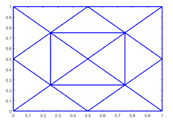
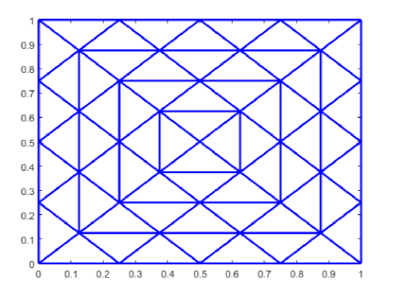
Figure 2: Triangulation used for computations in Examples 5.1-5.4

Table 1: Errors and convergence orders to the conforming FE solution of Example 5.1

$h$	$L_{2}$-error	Order	$H^{1}$-error	Order	$\left|\!\left|\!\left|\cdot\right|\!\right|\!\right|_{LPSD}$	Order
1/4	0.263770	-	1.540172	-	1.818878	-
1/8	0.080853	1.705905	0.847902	0.861120	0.711660	1.353788
1/16	0.021496	1.911176	0.320976	1.401432	0.180366	1.980258
1/32	0.004985	2.108176	0.125672	1.352791	0.054998	1.713475
1/64	0.001214	2.037217	0.056010	1.165911	0.018152	1.599241
1/128	0.000299	2.018018	0.025754	1.120875	0.006203	1.548898

Table 2: Errors and convergence orders to the nonconforming FE solution of Example 5.1

$h$	$L_{2}$-error	Order	$H^{1}$-error	Order	$\left|\!\left|\!\left|\cdot\right|\!\right|\!\right|_{LPSD}$	Order
1/4	0.218747	-	1.387872	-	0.796730	-
1/8	0.052263	2.065387	0.606678	1.193870	0.190189	2.066650
1/16	0.013520	1.950637	0.262326	1.209569	0.037488	2.342906
1/32	0.003466	1.963566	0.114017	1.202108	0.009396	1.996299
1/64	0.000897	1.950087	0.051673	1.141751	0.002739	1.778052
1/128	0.000219	2.031642	0.021006	1.298612	0.000835	1.712686

Figure 3: Nonconforming stabilized finite element solution (a) and the errors of GLPS finite element approximations (b) of the example (5.1).

Example 5.2

(Advection problem)
Consider the model problem (1) with $\Omega=(0,1)^{2}$, coefficients $\mathbf{b}=(0,1)$, $\mu=1$ and inflow boundary condition $g(x)=0$. The source term $f$ is chosen such that the solution

$$u(x,y)=\frac{1}{2}\left(\tanh\left(\frac{y-.5}{0.04}\right)+1\right)$$

satisfies the model problem. The stabilization parameters for conforming and nonconforming finite element approximations are chosen as $\beta_{a}=0.1h_{a}$ and $\beta_{E}=0.2h_{E}$ respectively.

Figure 4(a) and (b) show the nonconforming Galerkin and the nonconforming GLPS finite element solutions. We can observe that the spurious oscillation in Galerkin solution is suppressed in GLPS approximation. Further, Table 3 and Table 4 present the errors and convergence behavior of the conforming and nonconforming stabilized finite element solutions, respectively. Moreover, Figure 5 dipicts the obtained optimal order of convergence in both the conforming and the nonconforming approximations.

Figure 4: (a) Nonconforming Galerkin and (b) nonconforming stabilized finite element with $\beta_{E}=0.2h_{E}$ solutions of the example (5.2).

Table 3: Errors and orders of convergence of conforming FE solution of Example 5.2.

$h$	$L_{2}$-error	Order	$H^{1}$-error	Order	$\left|\!\left|\!\left|\cdot\right|\!\right|\!\right|_{LPSD}$	Order
1/4	1.8666	-	15.3910	-	6.3703	-
1/8	0.8769	1.0898	13.4262	0.1970	3.6031	0.8221
1/16	0.1677	2.3864	6.3194	1.0871	0.9101	1.9850
1/32	0.0223	2.9077	1.7178	1.8791	0.1878	2.2765
1/64	0.0042	2.3896	0.6164	1.4784	0.0565	1.7324
1/128	0.0010	2.0838	0.2921	1.0773	0.0155	1.8622
1/256	0.0002	2.0026	0.14534	1.0072	0.0048	1.6722

Table 4: Errors and orders of convergence of nonconforming FE solution of Example 5.2

$h$	$L_{2}$-error	Order	$H^{1}$-error	Order	$\left|\!\left|\!\left|\cdot\right|\!\right|\!\right|_{LPSD}$	Order
1/4	0.2057	-	5.5664	-	1.7495	-
1/8	0.1344	0.6135	3.4595	0.6861	0.6924	1.3372
1/16	0.0579	1.2153	1.9449	0.8308	0.2302	1.5882
1/32	0.0190	1.6052	0.9636	1.0131	0.0464	2.3098
1/64	0.0047	1.9983	0.4548	1.0829	0.0069	2.7484
1/128	0.0011	2.0198	0.2364	0.9440	0.0012	2.4467

Figure 5: Order of convergence of the stabilised finite element solution of the example 5.2.

Example 5.3

(Circular internal layer)
Consider the model problem (1) with $\Omega=(0,1)^{2}$, coefficients $\mathbf{b}=(2,3)$ and $\mu=2$. The source term $f$ and the inflow boundary condition are chosen such that the solution

$$u(x,y)=16x(1-x)y(1-y)\left(\frac{1}{2}+\frac{\tan^{-1}\left(200\left((0.25)^{2}-(x-.5)^{2}-(y-.5)^{2})\right)\right)}{\pi}\right)$$

satisfies the model equation. This solution possesses a circular internal layer on the circumference of the circle, centered at (0.5,0.5) and radius 0.25, in the unit square domain. The conforming and the nonconforming approximations are obtained with the stabilization parameters $\beta_{a}=0.06h_{a}$ and $\beta_{E}=0.05h_{E}$, respectively. Figure 6 (a) dipicts the GLPS conforming stabilised finite element solution on a mesh with $h=0.0078$. We can observe that the conforming stabilized scheme approximates the solution well and retains the solution’s inner circular layer. A similar result is obtained with the nonconforming GLPS finite element approximation. Figure 6 (b) presents the errors in the conforming and nonconforming approximations. Next, the Table 5 displays the errors in $\left|\!\left|\!\left|\cdot\right|\!\right|\!\right|_{LPSD}$ norm and the order of convergence for the GLPS conforming and nonconforming finite approximations and supports the theoretical estimates.

$h$		$1/4$	$1/8$	$1/16$	$1/32$	$1/64$	$1/128$
$V^{c}_{h}$	$\left|\!\left|\!\left|\cdot\right|\!\right|\!\right|_{LPSD}$	1.1680	4.0817	1.5967	0.91067	0.4164	0.1300
	Order	-	-1.8050	1.3540	0.8101	1.1288	1.67908
$V^{nc}_{h}$	$\left|\!\left|\!\left|\cdot\right|\!\right|\!\right|_{NLPSD}$	2.1939	2.6771	0.8502	0.3660	0.1516	0.0275
	Order	-	-0.2871	1.6546	1.2158	1.2713	2.4622

Table 5: Errors and convergence orders to the GLPS finite element approxomations of the example 5.3.

Figure 6: Conforming stabilized FE solution and its order of convergence of the example (5.3).

Example 5.4

(Non-smooth solution)
Consider the model problem (1) with $\Omega=(-1,1)^{2}$, coefficients $\mathbf{b}=(1,0)$, $\mu=0$, $f=0$, the inflow boundary condition

$$g(x)=\left\{\begin{array}[]{ll}1&\quad y>0\\ 0&\quad y<0,\end{array}\right.$$

and the exact solution

$$u(x,y)=\left\{\begin{array}[]{ll}1&\quad y>0\\ 0&\quad y<0.\end{array}\right.$$

Even though a discontinuous boundary data [16, Example 2] is not considered in our numerical analysis, this example is considered to examine the robustness of the proposed scheme. The stabilization parameters for the conforming and the nonconforming approximations are chosen as $\beta_{a}=0.7h_{a}$ and $\beta_{E}=0.7h_{E}$, respectively. Figure 7 dipicts the conforming and the nonconforming stabilized finite element solutions on a mesh with $h$= 0.015625. The boundary layers are not resolved, because the boundary conditions are imposed weakly in the current scheme. Nevertheless, with the generalized LP stabilization method, the interior layer is captured well. While small overshoots and undershoots are observed near the interior layer, there are no oscillations in the solution away from the layer and it shows the robustness of the proposed scheme.

Figure 7: Left side conforming stabilized solution and right side nonconforming stabilized solution of the example 5.4 with $h$= 0.015625.

6 Summary

We have derived stability and convergence estimates for the generalized local projection stabilized finite element scheme for advection-reaction equations with conforming and nonconforming interpolation spaces. In particular, optimal a priori error estimates are established for both the conforming and nonconforming approximations with respect to the local projection streamline derivative norm. The accuracy and the robustness of the proposed scheme are shown numerically with suitable examples. Moreover, extension of this study to flow problem is planned.

References

- [1] Claudio Baiocchi, Franco Brezzi, and Leopoldo P Franca. Virtual bubbles and Galerkin-least-squares type methods (Ga. L.S). Comput. Methods Appl. Mech. Engrg., 105(1):125–141, 1993.
- [2] Randolph E Bank and Harry Yserentant. On the -stability of the -projection onto finite element spaces. Numer. Math., 126(2):361–381, 2014.
- [3] Roland Becker and Malte Braack. A finite element pressure gradient stabilization for the Stokes equations based on local projections. Calcolo, 38(4):173–199, 2001.
- [4] Malte Braack and Erik Burman. Local projection stabilization for the Oseen problem and its interpretation as a variational multiscale method. SIAM J. Numer. Anal., 43(6):2544–2566, 2006.
- [5] James H Bramble, Joseph E Pasciak, and Olaf Steinbach. On the stability of the projection in . Math. Comp, 71(237):147–156, 2002.
- [6] James H Bramble and Alfred H Schatz. Rayleigh-Ritz-Galerkin methods for dirichlet’s problem using subspaces without boundary conditions. Comm. Pure Appl. Math., 23(4):653–675, 1970.
- [7] JH Bramble and AH Schatz. Least squares methods for 2mth order elliptic boundary-value problems. Math. Comp., 25(113):1–32, 1971.
- [8] Susanne C. Brenner and L Ridgway Scott. The mathematical theory of finite element methods. Springer-Verlag, New York, 2008.
- [9] Franco Brezzi, Thomas JR Hughes, LD Marini, Alessandro Russo, and Endre Süli. A priori error analysis of residual-free bubbles for advection-diffusion problems. SIAM J. Numer. Anal., 36(6):1933–1948, 1999.
- [10] Alexander N Brooks and Thomas JR Hughes. Streamline upwind/Petrov-Galerkin formulations for convection dominated flows with particular emphasis on the incompressible Navier-Stokes equations. Comput. Methods Appl. Mech. Engrg., 32(1-3):199–259, 1982.
- [11] Erik Burman. A unified analysis for conforming and nonconforming stabilized finite element methods using interior penalty. SIAM J. Numer. Anal., 43(5):2012–2033, 2005.
- [12] Erik Burman. A posteriori error estimation for interior penalty finite element approximations of the advection-reaction equation. SIAM J. Numer. Anal., 47(5):3584–3607, 2009.
- [13] Erik Burman and Alexandre Ern. A Continuous finite element method with Face penalty to approximate Friedrichs’ systems. M2AN Math. Model. Numer. Anal., 41(1):55–76, 2007.
- [14] Erik Burman and Alexandre Ern. Continuous interior penalty -finite element methods for advection and advection-diffusion equations. Math. Comput., 76(259):1119–1140, 2007.
- [15] Erik Burman and Peter Hansbo. Edge stabilization for Galerkin approximations of convection–diffusion–reaction problems. Comput. Methods Appl. Mech. Engrg., 193(15-16):1437–1453, 2004.
- [16] Erik Burman and Benjamin Stamm. Minimal stabilization for discontinuous Galerkin finite element methods for hyperbolic problems. J. Sci. Comput., 33:183–208, 2007.
- [17] Daniele Antonio Di Pietro and Alexandre Ern. Mathematical aspects of discontinuous Galerkin methods, volume 69. Springer Science & Business Media, 2011.
- [18] Asha K Dond and Thirupathi Gudi. Patch-wise local projection stabilized finite element methods for convection–diffusion–reaction problems. Numer. Methods Partial Differential Equations, 35(2):638–663, 2019.
- [19] AV Dzhishkariani. The least square and Bubnov–Galerkin methods. Russian Academy of Sciences, Branch of Mathematical Sciences, 8(5):1110–1116, 1968.
- [20] A Ern and JL Guermond. Theory and practice of finite elements springer-verlag. New York, 2004.
- [21] Sashikumaar Ganesan. An operator-splitting Galerkin/SUPG finite element method for population balance equations: stability and convergence. ESAIM Math. Model. Numer. Anal., 46(6):1447–1465, 2012.
- [22] Sashikumaar Ganesan, Gunar Matthies, and Lutz Tobiska. Local projection stabilization of equal order interpolation applied to the Stokes problem. Math. Comp., 77(264):2039–2060, 2008.
- [23] Sashikumaar Ganesan and Lutz Tobiska. Stabilization by local projection for convection–diffusion and incompressible flow problems. J. Sci. Comput., 43(3):326–342, 2010.
- [24] Thomas JR Hughes, Leopoldo P Franca, and Gregory M Hulbert. A new finite element formulation for computational fluid dynamics: VIII. the Galerkin/least-squares method for advective diffusive equations. Comput. Methods Appl. Mech. Engrg, 73:173–189, 1989.
- [25] V John, JM Maubach, and L Tobiska. Nonconforming streamline-diffusion-finite-element-methods for convection-diffusion problems. Numer. Math., 78(2):165–188, 1997.
- [26] Volker John, G Matthies, F Schieweck, and L Tobiska. A streamline-diffusion method for nonconforming finite element approximations applied to convection-diffusion problems. Comput. Methods Appl. Mech. Engrg., 166(1-2):85–97, 1998.
- [27] Petr Knobloch. A generalization of the local projection stabilization for convection-diffusion-reaction equations. SIAM J. Numer. Anal., 48(2):659–680, 2010.
- [28] Petr Knobloch and Lutz Tobiska. The element: A new nonconforming finite element for convection-diffusion problems. SIAM J. Numer. Anal., 41(2):436–456, 2003.
- [29] Petr Knobloch and Lutz Tobiska. Improved stability and error analysis for a class of local projection stabilizations applied to the Oseen problem. Numer. Methods Partial Differential Equations, 29(1):206–225, 2013.
- [30] Subhashree Mohapatra and Sashikumaar Ganesan. A non-conforming least squares spectral element formulation for Oseen equations with applications to Navier-Stokes equations. Numer. Funct. Anal. Optim., 37(10):1295–1311, 2016.
- [31] Kamel Nafa. Local projection finite element stabilization for Darcy flow. Int. J. Numer. Anal. Model., 7(4):656–666, 2010.
- [32] Lutz Tobiska. Finite element methods of streamline diffusion type for the Navier-Stokes equations. Numerical methods Miskolc, pages 259–266, 1990.
- [33] Lutz Tobiska and Rüdiger Verfürth. Analysis of a streamline diffusion finite element method for the Stokes and Navier–Stokes equations. SIAM J. Numer. Anal., 33(1):107–127, 1996.
- [34] J. Venkatesan and S. Ganesan. Finite element computations of viscoelastic two-phase flows using local projection stabilization. Int. J. Numer. Meth. Fluids, DOI: 10.1002/fld.4808, 2020.