Elemental Abundances in M31: Properties of the Inner Stellar Halo

Abstract

We present measurements of [Fe/H] and [$\alpha$/Fe] for 128 individual red giant branch stars (RGB) in the stellar halo of M31, including its Giant Stellar Stream (GSS), obtained using spectral synthesis of low- and medium-resolution Keck/DEIMOS spectroscopy ($R\sim 3000$ and 6000, respectively). We observed four fields in M31’s stellar halo (at projected radii of 9, 18, 23, and 31 kpc), as well as two fields in the GSS (at 33 kpc). In combination with existing literature measurements, we have increased the sample size of [Fe/H] and [$\alpha$/Fe] measurements to a total of 229 individual M31 RGB stars. From this sample, we investigate the chemical abundance properties of M31’s inner halo, finding $\langle$[Fe/H]$\rangle$ = $-$1.08 $\pm$ 0.04 and $\langle$[$\alpha$/Fe]$\rangle$ = 0.40 $\pm$ 0.03. Between 8–34 kpc, the inner halo has a steep [Fe/H] gradient ($-$0.025 $\pm$ 0.002 dex kpc^-1) and negligible [$\alpha$/Fe] gradient, where substructure in the inner halo is systematically more metal-rich than the smooth component of the halo at a given projected distance. Although the chemical abundances of the inner stellar halo are largely inconsistent with that of present-day dwarf satellite galaxies of M31, we identified 22 RGB stars kinematically associated with the smooth stellar halo that have chemical abundance patterns similar to M31 dSphs. We discuss formation scenarios for M31’s halo, concluding that these dSph-like stars may have been accreted from galaxies of similar stellar mass and star formation history, or of higher stellar mass and similar star formation efficiency.

1 Introduction

In the $\Lambda$CDM cosmological paradigm, $L_{\star}$ galaxies like the Milky Way (MW) and Andromeda (M31) form through hierarchical assembly (e.g., White & Rees 1978). Debris from mergers across cosmic time are deposited within the extended stellar halo, where they remain observationally identifiable because the phase-mixing timescales in the outskirts of galaxies are long compared to the age of the universe (e.g., Helmi et al. 1999; Bullock & Johnston 2005). Simulations of stellar halo formation in MW-like galaxies have shown that the mass and accretion time distributions of progenitor dwarf galaxies can imprint strong chemical signatures in a galaxy’s stellar population (e.g., Robertson et al. 2005; Font et al. 2006b; Johnston et al. 2008; Zolotov et al. 2010; Tissera et al. 2012), particularly in terms of [Fe/H] and [$\alpha$/Fe]. Measurements of $\alpha$-element abundance (O, Ne, Mg, Si, S, Ar, Ca, and Ti) and iron (Fe) abundance encode information concerning the relative timescales of Type Ia and core-collapse supernovae (e.g., Gilmore & Wyse 1998), such that galactic systems with different evolutionary histories will have distinct chemical abundance patterns. In this way, stellar halos serve as fossil records of a galaxy’s accretion history. This theory has been extensively put into practice in the MW, where the differing patterns of [$\alpha$/Fe] and [Fe/H] between its stellar halo and satellite dwarf galaxies have revealed their fundamentally incompatible enrichment histories (Shetrone et al., 2001; Venn et al., 2004).

Studies of the kinematics and chemical composition of individual stars in the MW have provided a detailed window into the formation of its stellar halo (e.g., Carollo et al. 2007, 2010; Nissen & Schuster 2010; Ishigaki et al. 2012; Haywood et al. 2018; Helmi et al. 2018; Belokurov et al. 2018, 2020). However, the MW is a single example of an $L_{\star}$ galaxy. Observations of MW-like stellar halos in the Local Volume have revealed a wide diversity in their properties, such as stellar halo fraction, mean photometric metallicity, and satellite galaxy demographics, which likely results from halo-to-halo variations in merger history (Merritt et al., 2016; Monachesi et al., 2016a; Harmsen et al., 2017; Geha et al., 2017; Smercina et al., 2019). In these studies, both the MW and M31 have emerged as outliers at the quiescent and active ends, respectively, of the spectrum of accretion histories for nearby $L_{\star}$ galaxies.

Owing to its proximity (785 kpc; McConnachie et al. 2005), M31 is currently the only $L_{\star}$ galaxy that we can study at a level of detail approaching what is possible in the MW. M31’s nearly edge-on orientation ($i=77^{\circ}$; de Vaucouleurs 1958) provides an exquisite view of its extended, highly structured stellar halo (e.g., Ferguson et al. 2002; Guhathakurta et al. 2005; Kalirai et al. 2006b; Gilbert et al. 2007, 2009b; Ibata et al. 2007, 2014; McConnachie et al. 2018). Most notably, M31’s stellar halo contains a prominent tidal feature known as the Giant Stellar Stream (GSS; Ibata et al. 2001), where the debris from this event litters the inner halo (Brown et al., 2006; Gilbert et al., 2007). Since the discovery of M31’s halo (Guhathakurta et al., 2005; Irwin et al., 2005; Gilbert et al., 2006), its global metallicity, and kinematical properties have been thoroughly characterized from photometric and shallow ($\sim$1 hr) spectroscopic surveys (Kalirai et al., 2006a; Ibata et al., 2007; Koch et al., 2008; McConnachie et al., 2009; Gilbert et al., 2012, 2014, 2018; Ibata et al., 2014). However, it is only recently that Vargas et al. (2014a, b) made the first chemical abundance measurements beyond metallicity estimates in M31’s halo and dwarf galaxies.

We have undertaken a deep ($\gtrsim$6 hour) spectroscopic survey using Keck/DEIMOS to probe the formation history of M31 from the largest sample of [Fe/H] and [$\alpha$/Fe] measurements in M31 to date. This has resulted in the first [$\alpha$/Fe] measurements in the GSS (Gilbert et al., 2019), the inner halo (Escala et al., 2019, 2020), and the outer disk (Escala et al., 2020), in addition to an expanded sample of [$\alpha$/Fe] and [Fe/H] measurements in M31 satellite galaxies (Kirby et al. 2020 for individual stars; Wojno et al. 2020 for coadded groups of spectra) and the outer halo (Gilbert et al., 2020). Some of our key results include (1) evidence for a high efficiency of star formation in the GSS progenitor (Gilbert et al., 2019; Escala et al., 2020) and the outer disk (Escala et al., 2020), (2) the distinct chemical abundance patterns of the inner halo compared to M31 satellite galaxies (Escala et al., 2020; Kirby et al., 2020), (3) support for chemical differences between the inner and outer halo (Escala et al., 2020; Gilbert et al., 2020), and (4) chemical similarity between MW and M31 satellite galaxies (Kirby et al., 2020; Wojno et al., 2020). In this contribution, we analyze the global chemical abundance properties of the kinematically smooth component of M31’s inner stellar halo.

This paper is organized as follows. In § 2, we present our recently observed M31 fields. We provide a brief overview of our chemical abundance analysis in § 3 and develop a statistical model to determine M31 membership in § 4. We present our [$\alpha$/Fe] and [Fe/H] measurements for 128 M31 RGB stars and analyze the combined sample of inner halo abundance measurements (including those in the literature) in § 5. Finally, we compare M31 to the MW and the Magellanic Clouds, and place our results in the context of stellar halo formation models in § 6.

2 Data

2.1 Spectroscopy and Data Reduction

Table 1 presents previously unpublished deep ($\gtrsim$ 5 hr) observations of six spectroscopic fields in M31. Fields f109_1, f123_1, f130_1, a0_1, a3_1, and a3_2 were observed in total for 7.0, 6.25, 6.74, 6.79, 6.44, and 6.60 hours, respectively. For five of these fields, we utilized the Keck/DEIMOS (Faber et al., 2003) 600 line mm^-1 (600ZD) grating with the GG455 order blocking filter, a central wavelength of 7200 Å, and 0.8” slitwidths. We observed a single field (f123_1) with the 1200 line mm^-1 (1200G) grating with the OG550 order blocking filter, a central wavelength of 7800 Å, and 0.8” slitwidths. We observed each spectroscopic field using two separate slitmasks that are identical in design, excepting slit position angles. This difference minimizes flux losses owing to differential atmospheric refraction at blue wavelengths via tracking changes in parallatic angle. The spectral resolution of the 600ZD (1200G) grating is approximately 2.8 (1.3) Å FWHM, or R$\sim$3000 (6500) at the Ca II triplet region ($\lambda\sim 8500$ Å). Similarly deep observations of DEIMOS fields in M31, which we further analyze in this work, were previously published by Escala et al. (2020, 2019) (600ZD) and Gilbert et al. (2019) (1200G).

One-dimensional spectra were extracted from the raw, two-dimensional DEIMOS data using the spec2d pipeline (Cooper et al., 2012; Newman et al., 2013), including modifications for bright, unresolved stellar sources (Simon, & Geha, 2007). Kirby et al. (2020) provides a comprehensive description of the data reduction process. We included additional alterations to correct for atmospheric refraction, which preferentially affects bluer optical wavelengths (Escala et al., 2019).

Figure 1: The location of deep ($\gtrsim$ 5 hr total exposure time) DEIMOS fields in M31-centric coordinates overlaid on the PAndAS red giant branch star count map (McConnachie et al., 2018). Rectangles represent the approximate size (16’ x 4’) and orientation of the DEIMOS fields, whereas the dashed magenta line corresponds to 50 projected kpc. We include fields observed with both the low-resolution (600ZD; magenta) and medium-resolution (1200G; green) gratings on DEIMOS. Nearby HST/ACS fields (202”x 202”; Brown et al. 2009) are shown as gold stars. Observations first presented in this work are outlined in white (Table 1; § 2). Our additional deep fields include 9 kpc, 18 kpc, 23 kpc, and 31 kpc in the stellar halo and 33 kpc in the Giant Stellar Stream.

Table 1: Deep DEIMOS Observations in M31

$\alpha_{\rm J2000}$	$\delta_{\rm J2000}$	P.A.	Grating	Slitmaska	Date	$\theta_{s}$ (′′)	$X$	$t_{\textrm{exp}}$ (hr)	$N$
f109_1 (9 kpc Halo Field)
00h45m47.02s	+40∘56${}^{{}^{\prime}}$58.7${}^{{}^{\prime\prime}}$	23.9	600ZD	f109_1a	2019 Oct 24	0.67	1.35	2.77	143
				f109_1a	2019 Oct 25	0.61	1.32	2.00	…
				f109_1b	2019 Oct 24	0.68	1.10	0.93	…
				f109_1b	2019 Oct 25	0.73	1.10	1.30	…
f123_1 (18 kpc Halo Field)
00h48m05.83s	+40∘27${}^{{}^{\prime}}$24.0${}^{{}^{\prime\prime}}$	$-$20	1200G	f123_1a	2017 Oct 23	0.88	1.52	2.83	136
				f123_1b	2019 Sep 25	0.80	1.34	3.42	…
f130_1 (23 kpc Halo Field)
00h49m11.90s	+40∘11${}^{{}^{\prime}}$50.3${}^{{}^{\prime\prime}}$	$-$20	600ZD	f130_1b	2019 Sep 25	0.43	1.07	1.15	93
				f130_1c	2018 Sep 10	0.72	1.29	0.97	…
				f130_1c	2018 Sep 11	0.80	1.25	2.07	…
				f130_1c	2019 Sep 25	0.61	1.25	2.55	…
a0_1 (31 kpc Halo Field)
00h51m51.31s	+39∘50${}^{{}^{\prime}}$26.9${}^{{}^{\prime\prime}}$	$-$17.9	600ZD	a0_1a	2019 Oct 24	0.68	1.07	0.73	67
				a0_1a	2019 Oct 25	0.57	1.06	0.43	…
				a0_1b	2019 Oct 24	0.66	1.24	2.84	…
				a0_1b	2019 Oct 25	0.70	1.24	2.79	…
a3_1 (33 kpc GSS Field)
00h48m22.09s	+39∘02${}^{{}^{\prime}}$33.1${}^{{}^{\prime\prime}}$	64.2	600ZD	a3_1a	2018 Sep 10	0.80	1.49	2.00	84
				a3_1a	2018 Sep 11	0.54	1.50	2.27	…
				a3_1a	2019 Sep 26	0.55	1.44	1.67	…
				a3_1b	2019 Sep 26	0.58	1.17	0.50	…
a3_2 (33 kpc GSS Field)
00h47m47.22s	+39∘05${}^{{}^{\prime}}$50.7${}^{{}^{\prime\prime}}$	178.2	600ZD	a3_2a	2018 Oct 02	0.60	1.16	2.10	80
				a3_2a	2019 Sep 26	0.64	1.09	1.00	…
				a3_2b	2019 Sep 26	0.61	1.18	3.50	…

• Note. — The columns of the table refer to right ascension, declination, position angle in degrees east of north, grating, slitmask name, date of observation (UT), average seeing, average airmass, exposure time per slitmask, and number of stars targeted per slitmask. Additional deep DEIMOS observations of M31 fields utilized in this work were published by Escala et al. (2019, 2020) and Gilbert et al. (2019).

• Slitmasks labeled as “a”, “b”, etc., are identical, except that the slits are tilted according to the parallactic angle at the approximate time of observation for the slitmask.

Figure 2: Extinction-corrected color-magnitude diagrams in the relevant photometric filters (Johnson-Cousins $V,I$ and CFHT/MegaCam $g,i$; § 2.3) for individual stars in each spectroscopic field (Table 1). For reference, we overplot PARSEC isochrones (black lines; Marigo et al. 2017), assuming 9 Gyr ages and [$\alpha$/Fe] = 0, with [Fe/H] = $-2.2$, $-1.0$, $-0.5$, and $0$ (from left to right). Stars without successful radial velocity measurements (§ 3) are represented as black points. Stars that are likely to be MW foreground dwarfs are indicated as grey diamonds, whereas likely M31 RGB stars (§ 4.1) are represented as circles.

2.2 Field Properties

Fields f109_1, f123_1, f130_1, a0_1, and a3 are located at 9, 18, 23, 31, and 33 kpc away from the galactic center of M31 in projected distance. We assumed that M31’s galactocenter is located at a right ascension of 0.71 hours and a declination of 41.3 degrees. Table 1 provides the mask center and mask position angle of each field on the sky. Figure 1 illustrates the locations of our newly observed DEIMOS fields relative to the center of M31, including previously observed fields (Escala et al., 2020, 2019; Gilbert et al., 2019) further analyzed in this work, overlaid on a RGB star count map from the Pan-Andromeda Archaeological Survey (PAndAS; McConnachie et al. 2018). We also show the locations of pencil-beam HST/ACS fields (Brown et al., 2009), some of which overlap with DEIMOS fields (Escala et al., 2020), from which Brown et al. (2006, 2007, 2008) derived stellar age distributions.

The deep fields presented in this work were previously observed using shallow ($\sim$1 hr) DEIMOS spectroscopy with the 1200G grating to obtain kinematical information for each field (Gilbert et al., 2007, 2009a). Based on the shallow 1200G observations, Gilbert et al. (2007, 2009a) argued that fields f109_1, f123_1, f130_1, and a0_1 probe the properties of the stellar halo of M31, whereas a3 probes the GSS. However, multiple kinematical components can be present in a given field. For example, f123_1 contains substructure known as the Southeast shelf, which is likely associated with the GSS progenitor (Gilbert et al., 2007; Fardal et al., 2007; Escala et al., 2020). Unlike fields along the GSS located closer to M31’s center, a3 does not show evidence for the secondary kinematically cold component (KCC) of unknown origin (Kalirai et al., 2006a; Gilbert et al., 2009a, 2019). We expect that f130_1 is associated with the “smooth”, relatively metal-poor halo of M31, based on the known properties of the overlapping DEIMOS field f130_2 (Figure 1; Escala et al. 2019). Similarly, the velocity distributions of a0_1 and f109_1 are fully consistent with that of M31’s stellar halo (Gilbert et al., 2007). Despite being the innermost M31 field in our sample ($r_{\rm proj}=9$ kpc, or $r_{\rm disk}=38$ kpc assuming $i$ = 77^∘), f109_1 does not show any kinematical evidence for significant contamination ($\gtrsim$10%) by M31’s extended disk (Gilbert et al., 2007). This also applies to the Southeast shelf, which was predicted to extend to the location of f109_1 with a large velocity dispersion ($\sim$350 km s^-1; Fardal et al. 2007; Gilbert et al. 2007), such that any hypothetical SE shelf stars in this field could not be kinematically separated from the halo population.

2.3 Photometry

The photometry for the majority of fields published in this work were obtained from MegaCam images in the $g^{\prime},i^{\prime}$ filters using the 3.6 m Canada-France-Hawaii Telescope (CFHT). The MegaCam images were obtained by Kalirai et al. (2006a) and reduced with the CFHT MegaPipe pipeline (Gwyn, 2008). For 9 targets in field f109_1 absent from our primary catalogs, we sourced g^′ and $i^{\prime}$ band photometry from the Pan-Andromeda Archaeological Survey (PAndAS) point source catalog (McConnachie et al., 2018). For field f130_1, the $g^{\prime}$, $i^{\prime}$ magnitudes were transformed to Johnson-Cousins $V,I$ using observations of Landolt photometric standard stars (Kalirai et al., 2006a). In the case of fields a0_1 and a3, the original photometry was obtained in the Washington $M,T_{2}$ filters by Ostheimer (2003) using the Mosaic camera on the 4 m Kitt Peak National Observatory (KPNO) telescope and subsequently transformed to the Johnson-Cousins $V,I$ bands using the relations of Majewski et al. (2000).

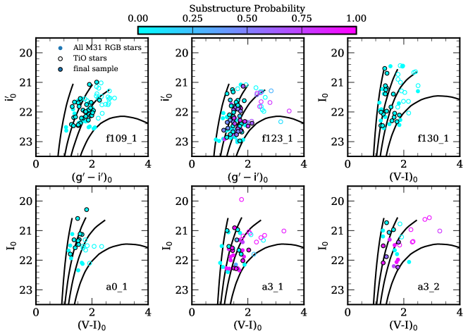
Figure 2 presents the extinction-corrected color-magnitude diagrams (CMDs) for each field in the relevant photometric filters used to derive quantities based on the photometry such as the photometric effective temperature ($T_{\rm{eff,phot}}$), surface gravity ($\log$ $g$), and metallicity ([Fe/H]_phot). We show all stars in a given field for which we extracted 1D spectra (M31 RGB stars, MW foreground dwarf stars, and stars for which we were unable to evaluate M31 membership owing to failed radial velocity measurements; § 4).

For fields f109_1, f130_1, a0_1, and a3, for which stellar spectra were obtained using the 600ZD grating (§ 2.1), we calculated $T_{\rm{eff,phot}}$, $\log$ $g$, and [Fe/H]_phot following the procedure described by Escala et al. (2020). In summary, the color and magnitude of a star are compared to a grid of theoretical stellar isochrones to derive the above quantities. We utilized the PARSEC isochrones (Marigo et al., 2017), which include molecular TiO in their stellar evolutionary modeling, and assumed a distance modulus to M31 of $m-M$ = 24.63 $\pm$ 0.20 (Clementini et al., 2011). For the 600ZD fields, we assumed 9 Gyr isochrones based on the mean stellar ages of the stellar halo and GSS, as inferred from HST CMDs

The photometric quantities ($T_{\rm{eff,phot}}$, $\log$ $g$) for the single 1200G-based field, f123_1, were derived following the procedure outlined by Kirby et al. (2008), assuming an identical distance modulus and 14 Gyr isochrones from a combination of model sets (Girardi et al., 2002; Demarque et al., 2004; VandenBerg et al., 2006). As described in detail by Escala et al. (2019) and summarized in § 5, $T_{\rm{eff,phot}}$ and $\log$ $g$ are used as constraints in measuring $T_{\rm{eff}}$, [Fe/H], and [$\alpha$/Fe] from spectra of individual stars, where these measurements are insensitive to the employed isochrone models and assumed stellar age.

3 Chemical Abundance Analysis

We use spectral synthesis of low- and medium-resolution stellar spectroscopy to measure stellar parameters ($T_{\rm{eff}}$) and abundances ([Fe/H] and [$\alpha$/Fe]) from our deep observations of M31 RGB stars. For a detailed description of the low- and medium-resolution spectral synthesis methods, see Escala et al. (2019, 2020) and Kirby et al. (2008), respectively. The low- and medium-resolution spectral synthesis procedures are nearly identical in principle, excepting differences in the continuum normalization given the differing wavelength coverage between the low- and medium-resolution spectra ($\sim$4500$-$9100 vs. 6300$-$9100 Å). For 1200G spectra, the continuum is determined using “continuum regions” defined by Kirby et al. (2008), whereas such regions would be unilaterally defined for 600ZD spectra owing to the high density of absorption features toward the blue wavelengths. Chemical abundances for individual stars measured using each technique are generally consistent within the uncertainties (Escala et al., 2020).

Prior to the chemical abundance analysis, the radial velocity of each star is measured via cross-correlation with empirical templates (Simon, & Geha, 2007; Kirby et al., 2015; Escala et al., 2020) observed in the relevant science configuration (§ 2.1). Systematic radial velocity errors of 5.6 km s^-1 (Collins et al., 2011) and 1.49 km s^-1 (Kirby et al., 2015) from repeat measurements of identical stars are added in quadrature to the random component of the error for observations taken with the 600ZD and 1200G gratings, respectively. The spectral resolution is empirically determined as a function of wavelength using the width of sky lines (Kirby et al., 2008), and in the case of the bluer 600ZD spectra, arc lines from calibration lamps (Escala et al. 2020; McKinnon et al., in preparation). The observed spectrum is then corrected for telluric absorption using a template of a hot star observed in the relevant science configuration (Kirby et al., 2008; Escala et al., 2019), shifted into the rest frame based on the measured radial velocity, and an initial continuum normalization is performed.

We measured the spectroscopic effective temperature, $T_{\rm{eff}}$, informed by photometric constraints, and fixed the surface gravity, $\log$ $g$, to the photometric value (§ 2.3). We simultaneously measured [Fe/H] and [$\alpha$/Fe] from regions of the spectrum sensitive to Fe and $\alpha$-elements (Mg, Si, Ca – with the addition of Ti for medium-resolution spectra), respectively, by comparing to a grid of synthetic spectra degraded to the resolution of the applicable DEIMOS grating (600ZD or 1200G) using Levenberg-Marquardt $\chi^{2}$ minimization. The grids of synthetic spectra utilized were generated for 4100$-$6300 Å and 6300$-$9100 Å, respectively, by Escala et al. (2019) and Kirby et al. (2008). The continuum determination is refined throughout this process, where $T_{\rm{eff}}$, [Fe/H], and [$\alpha$/Fe] are measured iteratively until $T_{\rm{eff}}$ changed by less than 1 K and [Fe/H] and [$\alpha$/Fe] each changed by less than 0.001. Finally, systematic errors on the abundances are added in quadrature to the random component of the error from the fitting procedure. For 600ZD-based abundance measurements, $\delta$([Fe/H])_sys = 0.130 and $\delta$([$\alpha$/Fe])_sys = 0.107, whereas for 1200G-based measurements, $\delta$([Fe/H])_sys = 0.101 and $\delta$([$\alpha$/Fe])_sys = 0.084 (Gilbert et al., 2019).

4 Membership Determination

Separating M31 RGB stars from the intervening foreground of MW dwarf stars has served as one of the primary challenges for spectroscopic studies of individuals stars in M31. The colors and heliocentric radial velocity distributions of MW and M31 stars exhibit significant overlap (e.g., Gilbert et al. 2006), thus the difficulty in disentangling the two populations when the distances to such faint stars are unknown. Early spectroscopic studies of M31 employed simple radial velocity cuts to exclude MW stars (e.g., Reitzel, & Guhathakurta 2002; Ibata et al. 2005; Chapman et al. 2006), resulting in kinematically biased populations of M31 RGB stars and relatively uncontaminated, albeit incomplete samples of M31 stars. Gilbert et al. (2006) performed the first rigorous, probabilistic membership determination in M31 using various diagnostics, including (1) heliocentric radial velocity, (2) the strength of the surface-gravity sensitive Na I $\lambda\lambda$8190 doublet, (3) CMD position, and (4) the discrepancy between photometric and calcium triplet based metallicity estimates as a distance indicator.

Given the variety of photometric filters utilized, Gilbert et al.’s method cannot be uniformly applied to all spectroscopic fields analyzed in this work. For inner halo fields ($r_{\rm proj}$ $\lesssim$ 30 kpc), Escala et al. (2020) illustrated that a binary membership determination using the aforementioned diagnostics is sufficient to recover the majority of stars classified as likely M31 RGB stars by the more sophisticated method of Gilbert et al. (2006) with minimal MW contamination. However, this binary determination excludes all stars with $v_{\rm helio}$ $>$ $-$150 km s^-1, where some of these stars may be M31 members at the positive tail of the stellar halo velocity distribution. It also does not allow us to assign a degree of certainty to our membership determination for each star. Thus, we used Bayesian inference to assign a membership probability to each observed star with a successful radial velocity determination (§ 3).

4.1 Membership Probability Model

We evaluated the probability of M31 membership for all stars with successful velocity measurements based on (1) a parameterization of color ($X_{\rm CMD}$), (2) the strength of the Na I absorption line doublet at $\lambda\lambda$8190 (EW_Na), (3) heliocentric radial velocity (§ 3; $v_{\rm helio}$), and (4) an estimate of the spectroscopic metallicity based on the strength of the calcium triplet ([Fe/H]_CaT).

Thus, according to Bayes’ theorem, the posterior probability that a star labeled by an index $j$ is an M31 member—given independent measurements $\vec{x_{j}}$ = (EW_Na,j, X_CMD,j, $v_{{\rm helio},j}$, [Fe/H]_CaT,j) with uncertainties $\delta\vec{x_{j}}$—is proportional to,

$$P({\rm M31}|\vec{x_{j}})\propto\\ P({\rm M31})_{j}\times P(\vec{x_{j}}|{\rm M31}),$$ (1)

where $P$(M31) is the prior probability that a star observed on a given DEIMOS slitmask is a member of M31, and $P(\vec{x_{j}}|$M31) is the likelihood of measuring a given set of membership diagnostics, $\vec{x_{j}}$, assuming the star is a M31 member. Analogously, we can also construct $P({\rm MW}|\vec{x_{j}})$, the posterior probability that a star belongs to the MW foreground population given a set of diagnostic measurements, where the sum of $P({\rm MW}|\vec{x}_{j})$ and $P({\rm M31}|\vec{x}_{j})$ is unity.

4.1.1 Measuring Membership Diagnostics

Figure 3: Properties of spectroscopically confirmed M31 (grey circles, purple contours) and MW (black crosses, blue contours) member stars from the SPLASH (Guhathakurta et al., 2005; Gilbert et al., 2006) survey. The contour levels correspond to 16^th, 50^th, and 84^th percentiles of the distributions. Histograms of star counts are also shown for both M31 and MW members. For clarity, we omit showing uncertainties in each parameter. The middle right panel illustrates the number of spectroscopically confirmed M31 members (Gilbert et al., 2006) relative to the number of targets with successful radial velocity measurements in a given field as a function of projected radius, , where we have fit the relationship with an exponential distribution, . We used heliocentric radial velocity ($v_{\rm helio}$), a parameterization of color ($X_{\rm CMD}$), Na I $\lambda\lambda 8190$ equivalent width (EW_Na), and calcium triplet metallicity estimates ([Fe/H]_CaT) as diagnostics to determine membership (§ 4.1.1, § 4.1.3) for our sample of stars with successful radial velocity measurements.

We described the CMD position of each star by the parameter $X_{\rm CMD}$, which is analogous to photometric metallicity ([Fe/H]_phot). The advantage of using $X_{\rm CMD}$ rather than color and magntiude is that we can place all of our stars on the same scale, despite the diversity of the photometric filter sets (§ 2.3). Assuming 12.6 Gyr isochrones and a distance modulus of 24.47, we defined $X_{\rm CMD}$ = 0 as the color of the most metal-poor PARSEC (Marigo et al., 2017) isochrone ([Fe/H] = $-$2.2) in the relevant photometric filter and $X_{\rm CMD}$ = 1 as the most metal-rich PARSEC isochrone ([Fe/H] = +0.5). Then, we used linear interpolation to map the color and magnitude of a star to a value of $X_{\rm CMD}$. The uncertainty on $X_{\rm CMD}$ was derived from the photometric errors by using a Monte Carlo procedure. This normalization provides the advantage of easily identifying stars that are bluer than the most metal-poor isochrone at a fixed stellar age by negative values of $X_{\rm CMD}$, where stars with $X_{\rm CMD}<0$ are $\gtrsim$10 times more likely to belong to the MW than M31 (Gilbert et al., 2006). In the sample being evaluated for membership, we classified stars with ($X_{\rm CMD}+\delta$X_CMD) $<$ 0 as MW dwarf stars.

By including [Fe/H]_CaT as an independent diagnostic in our model, we can additionally distinguish between foreground stars at unknown distances and distant giant stars. Given that our assumed distance modulus is appropriate only for stars at the distance of M31, [Fe/H]_phot, and analogously, $X_{\rm CMD}$, measurements are fundamentally incorrect for MW stars. Therefore, the two stellar populations will appear distinct in $X_{\rm CMD}$ versus [Fe/H]_CaT space. In order to compute [Fe/H]_CaT , we fit Gaussian profiles to 15 Å wide windows centered on Ca II absorption lines at 8498, 8542, and 8662 Å. Then, we calculated a total equivalent width for the calcium triplet from a linear combination of the individual equivalent widths,

$$\Sigma{\rm Ca}=0.5\times{\rm EW}_{\lambda 8498}+1.0\times{\rm EW}_{\lambda 8542}+0.6\times{\rm EW}_{\lambda 8662},$$ (2)

following Rutledge et al. (1997a). In addition to $\Sigma$Ca, the calibration to determine [Fe/H]_CaT depends on stellar luminosity,

$${\rm[Fe/H]_{CaT}}=-2.66+0.42\times\Sigma{\rm Ca}+0.27\times(V-V_{\rm HB}),$$ (3)

where $V-V_{\rm HB}$ is the Johnson-Cousins $V$-band apparent magnitude above the horizontal branch, assuming that $V_{\rm HB}$ = 25.17 for M31 (Holland et al., 1996) For fields with CFHT MegaCam $g^{\prime}$ and $i^{\prime}$ band photometry (§ 2.3), we approximated $V-V_{\rm HB}$ by $g^{\prime}-g^{\prime}_{\rm HB}$ using an empirical transformation between SDSS and Johnson-Cousins photometry (Jordi et al., 2006),

$$g-V=0.56\times(g-r+0.23)/1.05+0.12.$$ (4)

Assuming that $g-r$ = 0.6 and $g^{\prime}_{\rm HB}\approx g_{\rm HB}$, we obtained $g_{\rm HB}=V_{\rm HB}+(g-V)=25.73$ for stars in M31.

We measured EW_Na by summing the area under the best-fit Gaussian line profiles fit to the observed spectrum between 8178$-$8190, 8189$-$8200 Å with central wavelengths of 8183, 8195 Å using least-squares minimization. This parameter is sensitive to temperature and surface gravity (Schiavon et al., 1997), thus functioning as a discriminant between MW dwarf stars and M31 RGB stars.

4.1.2 Prior Probability of M31 Membership

Figure 4: Properties used as membership diagnostics ($v_{\rm helio}$, EW_Na, $X_{\rm CMD}$, [Fe/H]_CaT) for stars in our spectroscopic fields (Table 1) with successful radial velocity measurements (§ 3). We also include previously observed fields H, S, D, and f130_2 (Figure 1; Escala et al. 2020). For clarity, we omit showing measurement uncertainties. Each point is color-coded by its probability of belonging to M31 . The SPLASH distributions utilized in our probability model (§ 4.1) are underlaid as contours. For field D, we used a distinct velocity criterion owing to the presence of M31’s disk at $\sim-130$ km s^-1(Escala et al., 2020). We identified 328 (210) secure M31 RGB stars and 92 (75) secure MW dwarf stars across the spectroscopic fields presented in this (prior) work.

The probability of a given star observed on a DEIMOS slitmask belonging to M31, $P$(M31), increases with decreasing projected radial distance from the center of M31, owing to the increase in M31’s stellar surface density. The trend of increasing probability of M31 membership with decreasing projected radius is augmented compared to expectations from M31’s surface brightness profile (Courteau et al., 2011; Gilbert et al., 2012) by our photometric pre-selection of DEIMOS spectroscopic targets. These selection criteria are designed to include M31 members and exclude MW foreground stars. The photometry of the targets spans the magnitude range characteristic of M31 RGB stars (20 $<$ $I_{0}$ $<$ 22.5). We also considered narrow-band, Washington DDO51 photometry in the fields a0_1 and a3. The DDO51 filter isolates the Mg b triplet, which acts as discriminant between MW dwarf and M31 giant stars due to its sensitivity to surface gravity. We expect that an enhancement in the probability of observing an M31 RGB star owing to magnitude cuts is fairly uniform at a factor of $\lesssim$ 2 within $r_{\rm proj}$ $\lesssim$ 30 kpc (Gilbert et al., 2012), where the majority of our targets are located. For fields toward the outer halo, such as a0_1 and a3, DDO51-selection bias increases the likelihood of observing an M31 RGB star by a factor of 3$-$4 (Gilbert et al., 2012).

Thus, we parameterized P(M31) empirically using the ratio of the number of secure M31 RGB stars (Gilbert et al., 2006), $N_{\rm M31}$, to the number of targets with successful radial velocity measurements, $N_{\rm targets}$, from the Spectroscopic and Phomtometric Landscape of Andromeda’s Stellar Halo (SPLASH; Guhathakurta et al. 2005; Gilbert et al. 2006) survey. The SPLASH survey consists of tens of thousands of shallow ($\sim$1 hr exposures) DEIMOS spectra of stars along the line of sight toward M31’s halo, disk, and satellite dwarf galaxies (e.g., Kalirai et al. 2010; Tollerud et al. 2012; Dorman et al. 2012, 2015; Gilbert et al. 2012, 2014, 2018). In addition to $N_{\rm M31}$/$N_{\rm targets}$ as a function of radius, Figure 3 presents measurements of EW_Na, $X_{\rm CMD}$, $v_{\rm helio}$, and [Fe/H]_CaT for 1,510 secure M31 members and 1,794 secure MW members across 29 spectroscopic fields in M31’s stellar halo. We controlled for differences in methodology between this work and SPLASH by re-determining $X_{\rm CMD}$ homogeneously for the SPLASH data from the original Johnson-Cousins photometry and measuring [Fe/H]_CaT for our sample based on the same calibration (Rutledge et al., 1997a) used in SPLASH .

Based on this data, we approximated P(M31) by an exponential distribution,

$$P_{\rm M31}(r_{j})=\exp(-r_{j}/r_{p}),$$ (5)

where $r_{j}$ is the projected radius of a star from M31’s galactic center and $r_{p}$ = 45.5 kpc. Figure 3 includes $P_{\rm M31}(r)$ overlaid on the SPLASH survey data.

4.1.3 Likelihood of M31 Membership

Given the wealth of existing information on the properties of M31 RGB stars (and the MW foreground dwarf stars characteristic of our selection function) from the SPLASH survey, we assigned membership likelihoods to individual stars informed by this extensive data set. We described the likelihood that a star, $j$, with unknown membership belongs to M31 given its diagnostic measurements and uncertainties, ($\vec{x}_{j}$, $\delta\vec{x}_{j}$), as,

$$P(\vec{x_{j}},\delta\vec{x_{j}}|\mathrm{M31})=\frac{1}{N_{i}}\sum_{i=1}^{N_{i}}P(\vec{x_{j}}|\vec{\theta_{i}},\delta\vec{\theta_{i}}),$$ (6)

where ($\vec{\theta_{i}}$, $\delta\vec{\theta_{i}}$) is a set of four diagnostic measurements and uncertainties for a star, $i$, from the SPLASH survey that is a secure M31 member. The total number of secure SPLASH member stars, $N_{i}$, equals 1,510 (1,794) for M31 (the MW). The likelihood that a star, $j$, with unknown membership belongs to the MW, $P(\vec{x_{j}},\delta\vec{x_{j}}|\mathrm{MW})$, is defined analogously. Assuming normally distributed uncertainties, the log likelihood that a star, $j$, is a member of either M31 or the MW given a single set of SPLASH measurements, $i$, is a non-parametric, $N_{k}$-dimensional Gaussian distribution,

$$\ln{P(\vec{x_{j}},\delta\vec{x_{j}}|\vec{\theta_{i}},\delta\vec{\theta_{i}})}=-\frac{N_{k}}{2}\ln{2\pi}-\frac{1}{2}\sum_{k=1}^{N_{k}}\ln(\delta x_{j,k}^{2}+\delta\theta_{i,k}^{2})\\ -\frac{1}{2}\sum_{k=1}^{N_{k}}\frac{(x_{j,k}-\theta_{i,k})^{2}}{\delta x_{j,k}^{2}+\delta\theta_{i,k}^{2}},$$ (7)

where $k$ corresponds to a given membership diagnostic (EW_Na, $X_{\rm CMD}$, $v_{\rm helio}$, or [Fe/H]_CaT) and $N_{k}$ is the number of diagnostics utilized for a given star. For some stars in our sample, we were unable to measure EW_Na and/or [Fe/H]_CaT as a consequence of factors such as weak absorption, low S/N, or convergence failure in the Gaussian fit. For such stars, we excluded EW_Na and/or [Fe/H]_CaT as a diagnostic, such that $N_{k}$ = 2$-$3.

Finally, we computed the probability that a star is a M31 RGB candidate, as opposed to a MW dwarf candidate, from the odds ratio of the posterior probabilities (Eq. 1),

$$p_{\rm M31,j}=\frac{P({\rm M31}|\vec{x_{j}},\delta\vec{x_{j}})/P({\rm MW}|\vec{x_{j}},\delta\vec{x_{j}})}{1+P({\rm M31}|\vec{x_{j}},\delta\vec{x_{j}})/P({\rm MW}|\vec{x_{j}},\delta\vec{x_{j}})},$$ (8)

where the proportionality factor in Eq. 1 is equivalent for $P$(M31$|\vec{x}_{j},\delta\vec{x_{j}}$) and $P$(MW$|\vec{x}_{j},\delta\vec{x_{j}}$).

4.1.4 Results of Membership Determination

Figure 5: Heliocentric radial velocity distributions for stars with successful velocity measurements (§ 3) in each of the spectroscopic fields (Table 1). Grey histograms represent distributions for likely M31 RGB stars (§ 4.1), whereas black outlined histograms represent likely MW foreground dwarf stars. The systemic velocity of M31 ($v_{\rm sys}=-300$ km s^-1) is indicated by a dashed vertical line. The adopted velocity model for M31 RGB stars in each field (§ 4.2; Gilbert et al. 2018) is overplotted as a purple curve. Halo stars are present in each field, where they are distributed in a kinematically hot component centered near the systemic velocity. The velocity distributions of f109_1, f130_1, a0_1 are fully consistent with a “smooth” stellar halo. The Southeast shelf, a tidal feature potentially originating from the GSS progenitor (Fardal et al., 2007; Gilbert et al., 2007), is evident in f123_1, whereas the substructure in fields a3_1 a3_2 correspond to the GSS.

Figure 4 summarizes our membership determination for 426 total stars with successful radial velocity measurements across the six spectroscopic fields first presented in this work. The probability distribution is strongly bimodal, where the majority of stars are either secure ($p_{{\rm M31},j}$ $\gtrsim$ 0.75) M31 RGB ($N_{\rm M31}={328}$) or MW dwarf ($N_{\rm MW}$ = 92) candidates, excepting 6 stars with intermediate properties (0.5 $<$ $p_{{\rm M31},j}$ $\lesssim$ 0.75).

Figure 4 also includes a homogeneously re-evaluated membership determination for fields H, S, D, and f130_2 (Figure 1; Escala et al. 2020), which we further analyze in this work. Across these four fields, 346 stars have successful radial velocity measurements, 210 (75) of which are classified as secure M31 (MW) stars. In total, 61 stars in these fields have intermediate properties, most of which (60) are located in field D. Owing to the presence of M31’s northeastern disk at MW-like line-of-sight velocity ($v_{\rm helio}\sim-130$ km s^-1; Escala et al. 2020), we calculated M31 membership probabilities in D without the use of radial velocity as a diagnostic. Then, we classified all stars with ($v_{\rm helio}-\delta v_{\rm helio}$) $>$ $-$100 km s^-1 as MW contaminants, as in Escala et al. (2020).

In order to maximize our sample size across all spectroscopic fields, we considered stars that are more likely to belong to M31 than the MW ($p_{{\rm M31},j}>0.5$) to be M31 members in the following analysis. For stars in common between our dataset and SPLASH, we recovered 91.1% of stars classified as M31 RGB stars by Gilbert et al. (2006), where we used an equivalent definition of membership ($\langle L_{{\rm splash},j}\rangle$ $>$ 0). The excess MW contamination is 0.30%, in addition to the expected 2-5% from Gilbert et al.’s method. The 8.6% discrepancy results from stars at MW-like heliocentric velocities that we conservatively classified as MW stars, where these stars are considered M31 RGB stars in SPLASH.

4.2 Kinematics of M31 RGB Stars

Figure 5 illustrates the heliocentric radial velocity distributions for all stars with successful measurements (§ 5), including both M31 RGB stars and MW dwarf stars (§ 4.1), across the spectroscopic fields. We also show the adopted Gaussian mixture models (Gilbert et al., 2018) describing the velocity distribution for each field, which were computed using over 5,000 spectroscopically confirmed M31 RGB stars across 50 fields in M31’s stellar halo. Gilbert et al. omitted radial velocity as a membership diagnostic (§ 4) in their analysis and simultaneously fit for contributions from M31 and MW components to obtain kinematically unbiased models for each field. Table 5.1 presents the parameters characterizing the velocity model for each field, where we assumed 50^th percentile values of Gilbert et al.’s marginalized posterior probability distribution functions. For the stellar halo components, we transformed the mean velocity from the Galactocentric to heliocentric frame using the median right ascension and declination of all stars in a given field (Gilbert et al., 2018).

We confirmed that the observed velocity distribution for each field is consistent with its velocity model using a two-sided Kolmogorov-Smirnov test. As discussed in § 2.2, f109_1, f130_1, and a0_1 probe the “smooth” stellar halo of M31 with no detected substructure, whereas fields f123_1 and a3 show clear evidence of substructure known to be associated with the Southeast shelf (Fardal et al., 2007; Gilbert et al., 2007, 2019; Escala et al., 2020) and the GSS. Owing to the spatial proximity (Figure 1) and kinematical similarity (Gilbert et al., 2007, 2009a, 2018) between fields f130_1 (this work) and f130_2 (Escala et al., 2020, 2019) and fields a3 (this work), we consider them together in our subsequent abundance analysis (§ 5).

4.2.1 Substructure Probability

Figure 6: [$\alpha$/Fe] versus [Fe/H] for M31 RGB stars in the spectroscopic fields (Table 1), color-coded according to the probability of belonging to substructure (Eq. 9; § 4.2.1). The final sample selection criteria are described in § 5.1. Stars belonging to the stellar halo are $\alpha$-enhanced on average, but span a wide range of [$\alpha$/Fe]. Most notably, $\alpha$-poor stars ([$\alpha$/Fe] $\lesssim$ 0) are consistently present in the stellar halo of M31.

Based on the velocity model for each field, we assigned a probability of belonging to substructure in M31’s stellar halo, $p_{\rm sub}$, to every star identified as a likely RGB candidate ($p_{\rm M31}$ $>$ 0.5; Eq. 8). For smooth stellar halo fields, $p_{\rm sub}$ = 0. For fields with substructure, we computed $p_{\rm sub}$ using an equation analogous to Eq. 8, where the Bayesian odds ratio is substituted with the relative likelihood that a M31 RGB star belongs to substructure versus the halo,

$$\mathcal{L}_{{\rm sub},j}=\frac{f_{\rm sub}\mathcal{N}(v_{j}|\mu_{\rm sub},\sigma_{\rm sub}^{2})}{f_{\rm halo}\mathcal{N}(v_{j}|\mu_{\rm halo},\sigma_{\rm halo}^{2})},$$ (9)

where $v_{j}$ is the heliocentric velocity of an individual star and $\mu$, $\sigma$, and $f$ are the mean, standard deviation, and fractional contribution of the substructure or halo component in the Gaussian mixture describing the velocity distribution for a given field. In contrast, Escala et al. (2020) calculated $p_{\rm sub}$ based on the full posterior distributions, as opposed to 50^th percentiles alone, of their velocity models for fields with kinematical substructure. Given that we included abundance measurements of M31 RGB stars from Escala et al. (2020) in this work, we re-calculated $p_{\rm sub}$ for such fields (H, S, and D; Figure 1) based on their 50^th percentiles, as above. In the following abundance analysis (§ 5), we incorporated $p_{\rm sub}$ as a weight when determining the chemical properties of the stellar halo.

5 The Chemical Properties of the Inner Stellar Halo

We measured [Fe/H] and [$\alpha$/Fe] for 128 M31 RGB stars across six spectroscopic fields spanning $8-34$ kpc in the stellar halo. We measured [Fe/H] for 80 additional RGB stars for which we could not measure [$\alpha$/Fe]. In combination with measurements from previous work by our collaboration (Escala et al., 2020; Gilbert et al., 2019, 2020), we have increased the sample size of individual [$\alpha$/Fe] and [Fe/H] measurements in M31 to 229 RGB stars.

Figure 6 shows [Fe/H] and [$\alpha$/Fe] measurements for each field, where we have color-coded each star according to its probability of belonging to substructure (Eq. 9; § 4.2.1). Table 5.1 summarizes the chemical properties for each kinematical component present in a given field, including previously published inner halo fields with abundance measurements (Escala et al., 2019, 2020; Gilbert et al., 2019). We calculated each average chemical property from a bootstrap resampling of 10⁴ draws of the final sample for each field, including weighting by the inverse square of the measurement uncertainty and the probability that a star belongs to a given kinematical component (§ 4.2.1).

Hereafter, we predominantly restricted our abundance analysis to RGB stars (§ 4.1) from all six fields that are likely to be dynamically associated with the kinematically hot stellar halo of M31. Additionally, we incorporated likely M31 halo stars from inner halo fields with existing abundance measurements (Escala et al., 2020; Gilbert et al., 2019) into our final sample. We will analyze the chemical composition of RGB stars likely belonging to substructure, such as the Southeast shelf (f123_1) and outer GSS (a3), in a companion study (I. Escala et al., in preparation). A catalog of stellar parameters and abundance measurements for M31 RGB stars in the six spectroscopic fields is presented in Appendix A.

5.1 Sample Selection and Potential Biases

Figure 7: Same as Figure 2, except showing only M31 RGB stars for each field. Points are color-coded according to their probability of belonging to kinematical substructure in the stellar halo (§ 4.2.1, Eq. 9). Open circles indicate M31 RGB stars with strong TiO absorption, which we excluded from our final sample (§ 5.1).

Table 2: Kinematical^a and Chemical^b Properties of M31 Fields

Field	$r_{\rm proj}$
	Comp.	$\mu$
	$\sigma$	(km s-1)
	$f$	$\langle$[Fe/H]$\rangle$	$\sigma$([Fe/H])	$\langle$[$\alpha$/Fe]$\rangle$	$\sigma$([$\alpha$/Fe])	N[α/Fe]
f109_1	9	Halo	$-$315.7	108.2	1.0	$-$0.93${}^{+0.08}_{-0.09}$	0.45 $\pm$ 0.09	0.32 $\pm$ 0.08	0.36${}^{+0.04}_{-0.05}$	30
H	12	Halo	$-$315.1	108.2	0.44	$-$1.30 $\pm$ 0.11	0.45${}^{+0.07}_{-0.08}$	0.45${}^{+0.12}_{-0.13}$	0.42${}^{+0.09}_{-0.14}$	16
		SE Shelf	$-$295.4	65.8	0.56	$-$1.30${}^{+0.13}_{-0.12}$	0.49${}^{+0.08}_{-0.09}$	0.53${}^{+0.08}_{-0.10}$	0.36${}^{+0.09}_{-0.11}$
f207_1	17	Halo	$-$319.6	98.1	0.35	$-$1.04${}^{+0.09}_{-0.07}$	0.26 $\pm$ 0.04	0.53 $\pm$ 0.07	0.16 $\pm$ 0.04	21
		GSS	$-$529.4	24.5	0.33	$-$0.87${}^{+0.09}_{-0.10}$	0.31 $\pm$ 0.06	0.44${}^{+0.04}_{-0.05}$	0.16 $\pm$ 0.03
		KCC	$-$427.3	21.0	0.32	$-$0.79 $\pm$ 0.07	0.20 $\pm$ 0.04	0.54 $\pm$ 0.06	0.14 $\pm$ 0.02
f123_1	18	Halo	$-$318.2	98.1	0.68	$-$1.00 $\pm$ 0.06	0.36 $\pm$ 0.04	0.40 $\pm$ 0.04	0.23 $\pm$ 0.03	49
		SE Shelf	$-$279.9	11.0	0.32	$-$0.71 $\pm$ 0.07	0.32${}^{+0.04}_{-0.05}$	0.41${}^{+0.04}_{-0.05}$	0.23 $\pm$ 0.04
S	22	Halo	$-$318.8	98.1	0.28	$-$0.66${}^{+0.16}_{-0.18}$	0.44${}^{+0.07}_{-0.10}$	0.49${}^{+0.05}_{-0.06}$	0.21${}^{+0.05}_{-0.04}$	20
		GSS	$-$489.0	26.1	0.49	$-$1.02${}^{+0.15}_{-0.14}$	0.45${}^{+0.10}_{-0.11}$	0.38${}^{+0.17}_{-0.19}$	0.45${}^{+0.07}_{-0.08}$
		KCC	$-$371.6	17.6	0.22	$-$0.71 $\pm$ 0.11	0.27 $\pm$ 0.09	0.35${}^{+0.08}_{-0.09}$	0.18${}^{+0.04}_{-0.05}$
f130c	23	Halo	$-$317.3	98.1	1.0	$-$1.64 $\pm$ 0.11	0.59${}^{+0.08}_{-0.07}$	0.39${}^{+0.09}_{-0.10}$	0.38${}^{+0.06}_{-0.09}$	30
D	26	Halo	$-$317.1	98.0	0.57	$-$1.00${}^{+0.17}_{-0.19}$	0.68${}^{+0.12}_{-0.14}$	0.55 $\pm$ 0.13	0.40${}^{+0.06}_{-0.08}$	23
		Disk	$-$128.4	16.2	0.43	$-$0.82 $\pm$ 0.09	0.28${}^{+0.07}_{-0.09}$	0.60${}^{+0.09}_{-0.10}$	0.28${}^{+0.05}_{-0.06}$
a0_1	31	Halo	$-$314.0	98.0	1.0	$-$1.35 $\pm$ 0.10	0.33${}^{+0.06}_{-0.07}$	0.40 $\pm$ 0.10	0.30 $\pm$ 0.07	10
a3c	33	Halo	$-$331.7	98.0	0.44	$-$1.48${}^{+0.12}_{-0.13}$	0.45${}^{+0.06}_{-0.07}$	0.41${}^{+0.05}_{-0.07}$	0.24 $\pm$ 0.06	21
		GSS	$-$444.6	15.7	0.56	$-$1.11${}^{+0.12}_{-0.13}$	0.46${}^{+0.06}_{-0.07}$	0.34${}^{+0.08}_{-0.09}$	0.30 $\pm$ 0.05

• Note. — The columns of the table correspond to field name, projected radial distance from the center of M31, kinematical component, mean heliocentric velocity, velocity dispersion, fractional contribution of the given kinematical component, mean [Fe/H], spread in [Fe/H], mean [$\alpha$/Fe], spread in [$\alpha$/Fe], and total number of RGB stars in a given field with [$\alpha$/Fe] measurements (regardless of component association). Chemical properties were calculated from a bootstrap resampling of the final sample, including weighting by the inverse variance of the measurement uncertainty and the probability that a star belongs to a given kinematical component.

• The parameters of the velocity model are the 50^th percentiles of the marginalized posterior probability distribution functions. These were computed by Gilbert et al. (2018) for all fields except H, S, and D. We have transformed the 50^th percentile values for the stellar halo components from the Galactocentric to heliocentric frame, based on the median right ascension and declination of all stars in a given field. For fields H, S, and D, Escala et al. (2020) fixed the stellar halo component to the parameters derived by Gilbert et al. (2018) to independently compute the posterior distributions.

• Chemical abundances for fields f109_1, f123_1, f130_1, a0_1, and a3 are first presented in this work. We have included chemical properties of previously published M31 fields H, S, D, and f130_2 (Escala et al., 2019, 2020) and f207_1 (Gilbert et al., 2019) for reference. We further analyze the halo populations of H, S, f130_2, and f207_1 in this work.

• We combined the chemical abundance samples for fields f130_1 (this work) and f130_2 (Escala et al., 2019, 2020) given their proximity (Figure 1) and the consistency of their velocity distributions (Gilbert et al., 2007, 2018). The same is true for fields a3_1 and a3_2 (this work), where Gilbert et al. (2009a, 2018) illustrated the similarity in kinematics between these fields.

We vetted our final sample to consist only of reliable abundance measurements (§ 3) for M31 RGB stars. Similar to Escala et al. (2019, 2020), we restrict our analysis to M31 RGB stars with $\delta$($T_{\rm{eff}}$) $<$ 200 K, $\delta$([Fe/H])  $<$ 0.5, $\delta$([$\alpha$/Fe])  $<$ 0.5, and well-constrained parameter estimates based on the 5$\sigma$ $\chi^{2}$ contours for all fitted parameters ($T_{\rm{eff}}$, [Fe/H], and [$\alpha$/Fe]). We also require that convergence is achieved in each of the measured parameters (§ 3). Unreliable abundance measurements often result from an insufficient signal-to-noise (S/N) ratio, translating to an effective S/N threshold of $\gtrsim$ 8 Å^-1 for robust measurements of [Fe/H] and [$\alpha$/Fe]. Such S/N limitations result in a bias in our final sample against metal-poor stars with low S/N spectra, but do not affect the [$\alpha$/Fe] distributions. This bias is negligible for our innermost halo fields (f109_1, f123_1), whereas it is on the order of 0.10$-$0.15 dex for our remaining fields (f130_1, a0_1, a3).

We also manually inspected spectra to exclude stars with clear signatures of strong molecular TiO absorption in the wavelength range 7055$-$7245 Å from our final sample. It is unclear whether abundances measured from TiO stars are accurate owing to the lack of (1) the inclusion of TiO in our synthetic spectral modeling (Kirby et al., 2008; Escala et al., 2019) and (2) an appropriate calibration sample. For stars with successful radial velocity measurements, 31.5%, 16.7%, 34.5%, 32.5%, 30.4%, and 31.3% of stars in fields f109_1, f123_1, f130_1, a0_1, a3_1, and a3_2 have clear evidence of TiO in their spectra. To be conservative, we excluded 54 M31 RGB stars that showed TiO but otherwise would have made the final sample. In total, 128 M31 RGB stars across the six spectroscopic fields pass the above selection criteria, thereby constituting our final sample.

As discussed in detail by Escala et al. (2020), removing stars on the basis of TiO results in a bias against stars with red colors, which translates to a bias in photometric metallicity ([Fe/H]_phot) against metal-rich stars. Including the sample presented in this work, this photometric bias ([Fe/H]_phot,mem $-$ [Fe/H]_phot,final) ranges from 0.13$-$0.40 dex per field. For fields a3, more stars kinematically associated with the GSS (§ 4.2) show evident TiO absorption, whereas for field f123_1, fewer stars in the Southeast shelf substructure are affected compared to those in the halo. Therefore, the exclusion of TiO stars disproportionately impacts the [Fe/H]_phot bias depending on the given field and kinematical component. However, a bias in [Fe/H]_phot cannot be converted into a bias in spectroscopic [Fe/H], considering that [Fe/H]_phot measurements suffer from degeneracy with stellar age and [$\alpha$/Fe] from which spectroscopic [Fe/H] measurements are exempt.

5.2 Abundance Distributions for Individual Fields

In this section, we provide a brief overview of the chemical abundance properties of the six spectroscopic fields first presented in this work (Table 1; Figure 1). We discuss the global properties of the inner stellar halo in § 5.3 and § 5.4.

• f109_1 (9 kpc halo field): Field f109_1 is the innermost region of the stellar halo of M31 yet probed with chemical abundances (Gilbert et al., 2007, 2014). It does not contain any detected kinematical substructure (§ 2.2, 4.2). Excepting fields along the GSS, which have an insufficient number of smooth halo stars to constrain the abundances of the stellar halo component, f109_1 is more metal-rich on average ($\langle$[Fe/H]$\rangle$ = $-$0.93${}^{+0.08}_{-0.09}$) than the majority of halo components in fields at larger projected distance (Table 5.1; see also § 5.3). Based on the abundances for this field, the inner halo of M31 may be potentially less $\alpha$-enhanced on average ($\langle$[$\alpha$/Fe]$\rangle$ = +0.32 $\pm$ 0.08) than the stellar halo at larger projected distances, although we did not measure a statistically significant [$\alpha$/Fe] gradient in M31’s inner stellar halo (§ 5.3). Additionally, we did not find evidence for a correlation between [Fe/H] and [$\alpha$/Fe] for this field, where we computed a distribution of correlation coefficients from 10⁵ draws of the measured abundances perturbed by their (Gaussian) uncertainties.

• f123_1 (18 kpc halo field): Field f123_1 is dominated by the smooth stellar halo, but it also has a clear detection of substructure (§ 4.2; Table 5.1) known as the Southeast shelf (§ 2.2; Fardal et al. 2007; Gilbert et al. 2007). We defer further analysis of this component to a companion paper (I. Escala et al., in preparation) owing to its likely connection to the GSS. The stellar halo in this field is metal-rich ($\langle$[Fe/H]$\rangle$ = $-$0.98 $\pm$ 0.05), $\alpha$-enhanced ($\langle$[$\alpha$/Fe]$\rangle$ = $+$0.41${}^{+0.03}_{-0.04}$), and exhibits no statistically significant correlation between [$\alpha$/Fe] and [Fe/H].

• f130_1 (23 kpc halo field): Similar to f109_1, f130_1 does not possess detectable substructure. We combined the chemical abundance samples for this field with f130_2 (Escala et al., 2019, 2020) due to their proximity (Figure 1) and the consistency of their velocity distributions (Gilbert et al., 2007, 2018). The average abundances for the combined sample of 30 M31 RGB stars ($\langle$[Fe/H]$\rangle$ = $-$1.64 $\pm$ 0.11, $\langle$[$\alpha$/Fe]$\rangle$ = $+$0.39${}^{+0.09}_{-0.10}$; Table 5.1) agree within the uncertainties with previous determinations from an 11 star sample by Escala et al. (2019, 2020). The lack of a significant trend between [$\alpha$/Fe] and [Fe/H] is also maintained by the larger sample. The inner halo at 23 kpc appears to be more metal-poor and $\alpha$-enhanced than field f109_1 at 9 kpc, possibly representing a population that assembled rapidly at early times (Escala et al., 2019). The star formation history inferred for this region of M31’s halo indicates that the majority of the stellar population is over 8 Gyr old (Brown et al., 2007), suggesting that an accretion origin would require the progenitor galaxies to have quenched their star formation at least 8 Gyr ago.

• a0_1 (31 kpc halo field): The stellar population at the location of a0_1 is solely associated with the kinematically hot component of the stellar halo (§ 4.2). The 10 RGB star sample in this field suggests a positive trend between [$\alpha$/Fe] and [Fe/H] ($r$ = 0.24${}^{+0.12}_{-0.24}$) that is likely a consequence of small sample size. Despite its similar projected distance from the center of M31 and kinematical profile, a0_1 appears to be more metal-rich ($\langle$[Fe/H]$\rangle$ = $-$1.35 $\pm$ 0.10) than f130, although it may be comparably $\alpha$-enhanced (Table 5.1). Nearby HST/ACS fields at 35 kpc (Figure 1) imply a mean stellar age of 10.5 Gyr (Brown et al., 2008) for the vicinity, compared to a mean stellar age of 11.0 Gyr at 21 kpc . The full age distributions suggest that the stellar populations are in fact distinct between the 21 and 35 kpc ACS fields: the star formation history of the 35 kpc field is weighted toward more dominant old stellar populations and is inconsistent with the star formation history at 21 kpc at more than 3$\sigma$ significance (Brown et al., 2008). If applicable to a0_1, this suggests that its stellar population is both younger and more metal-rich than that at 23 kpc .

• a3 (33 kpc GSS fields): Field a3 is dominated by GSS substructure (§ 2.2, § 4.2), such that it may not provide meaningful constraints on the smooth stellar halo in this region. However, the stellar halo at 33 kpc along the GSS may be more metal-poor ($\langle$[Fe/H]$\rangle$ = $-$1.48${}^{+0.12}_{-0.13}$) than at 17 and 22 kpc along the GSS (Table 5.1). The abundances in this field clearly show a declining pattern of [$\alpha$/Fe] with [Fe/H], which is characteristic of dwarf galaxies. A comparison between $\langle$[Fe/H]$\rangle$ for the GSS between fields f207_1 and S indicates that the GSS likely has a metallicity gradient, as found from photometric based metallicity estimates (Ibata et al., 2007; Gilbert et al., 2009a; Conn et al., 2016; Cohen et al., 2018). We will quantify spectral synthesis based abundance gradients in the GSS and make connections to the properties of the progenitor in future work (I. Escala et al., in preparation).

In agreement with previous findings (Escala et al., 2019, 2020; Gilbert et al., 2019), the M31 fields are $\alpha$-enhanced with a significant spread in metallicity. This implies that stars in the inner stellar halo formed rapidly, such that the timescale for star formation was less than the typical delay time for Type Ia supernovae. For an accreted halo, a spread in metallicity coupled with high $\alpha$-enhancement can indicate contributions from multiple progenitor galaxies or a dominant, massive progenitor galaxy with high star formation efficiency (Robertson et al., 2005; Font et al., 2006b; Johnston et al., 2008; Font et al., 2008). We further discuss formation scenarios for M31’s stellar halo in § 6.3.

5.3 The Inner vs. Outer Halo

Figure 8: [Fe/H] (left) and [$\alpha$/Fe] (right) versus projected distance from the center of M31 for 197 M31 RGB stars (Escala et al. 2019, 2020; Gilbert et al. 2019; this work) in the inner halo ($r_{\rm proj}$ $\lesssim$ 35 kpc). Stars are color-coded according to their probability of substructure association (§ 4.2.1). We omit measurement uncertainties for clarity. $\langle$[Fe/H]$\rangle$ and $\langle$[$\alpha$/Fe]$\rangle$ for the halo component in each spectroscopic field (Table 5.1) are plotted as indigo diamonds. The photometric metallicity gradient of the stellar halo ($t$ = 10 Gyr, [$\alpha$/Fe] = 0) measured from spectroscopically confirmed M31 RGB stars (Gilbert et al., 2014) is indicated as a dotted gold line, assuming an intercept of [Fe/H]_phot = $-$0.5. This slope is unchanged within the uncertainties with the inclusion/exclusion of substructure. We also display [Fe/H]_phot gradients measured from our final spectroscopic sample (dotted black and brown lines). The uncertainty envelopes are determined from 16^th and 84^th percentiles.

The existence of a steep, global metallicity gradient in M31’s stellar halo is well-established from both Ca triplet based (Koch et al., 2008) and photometric (Kalirai et al., 2006b; Ibata et al., 2014; Gilbert et al., 2014) metallicity estimates. In addition to radial [Fe/H] gradients, the possibility of radial [$\alpha$/Fe] gradients between the inner and outer halo of M31 has recently been explored. From a sample of 70 M31 RGB stars, including an additional 21 RGB stars from Gilbert et al. (2019), with spectral synthesis based abundance measurements, Escala et al. (2020) found tentative evidence that the inner stellar halo ($r_{\rm proj}$ $\lesssim$ 26 kpc) had higher $\langle$[$\alpha$/Fe]$\rangle$ than a sample of four outer halo stars (Vargas et al., 2014b) drawn from $\sim$70$-$140 kpc. Gilbert et al. (2020) increased the number of stars in the outer halo (43$-$165 kpc) with abundance measurements from four to nine. In combination with existing literature measurements by Vargas et al. (2014b), Gilbert et al. found that $\langle$[$\alpha$/Fe]$\rangle$ = 0.30 $\pm$ 0.16 for the outer halo. This value is formally consistent with the average $\alpha$-enhancement of M31’s inner halo from the 91 M31 RGB star sample ($\langle$[$\alpha$/Fe]$\rangle$ = 0.45 $\pm$ 0.06), indicating an absence of a gradient between the inner and outer halo, with the caveat that the sample size in the outer halo is currently limited.

Despite the formal agreement between $\langle$[$\alpha$/Fe]$\rangle$ in the inner and outer halo, Gilbert et al. found that [Fe/H] and [$\alpha$/Fe] measurements of M31’s outer halo are similar to those of M31 satellite dwarf galaxies (Vargas et al., 2014a; Kirby et al., 2020) and the MW halo (e.g., Ishigaki et al., 2012; Hayes et al., 2018). In comparison, [$\alpha$/Fe] is higher at fixed [Fe/H] in M31’s inner halo than in its dwarf galaxies (Escala et al., 2020). This suggests that M31’s outer halo may have a more dominant population of stars with lower [$\alpha$/Fe] than the inner halo. This difference implies that the respective stellar halo populations may be, in fact, distinct.

With the contribution from this work of 128 M31 individual RGB stars to the existing sample of literature [Fe/H] and [$\alpha$/Fe] measurements (Vargas et al., 2014b; Escala et al., 2019, 2020; Gilbert et al., 2019, 2020), we obtaining $\langle$[Fe/H]$\rangle$ = $-$1.08 $\pm$ 0.04 ($-$1.17 $\pm$ 0.04) and $\langle$[$\alpha$/Fe]$\rangle$ = 0.40 $\pm$ 0.03 (0.39 $\pm$ 0.04) for M31’s inner halo when excluding (including) substructure. From this enlarged sample of inner halo abundance measurements, we assessed the presence of gradients in [Fe/H] and [$\alpha$/Fe] over the radial range spanned by our spectroscopic sample (8–34 kpc).

Taking stars in the kinematically hot stellar halo to have $p_{\rm sub}$ $<$ 0.5 (Eq. 9), we identified 122 (75) stars that are likely associated with the “smooth” stellar halo (kinematically cold substructure) within a projected distance of $r_{\rm proj}$ $\lesssim$ 35 kpc of M31. We emphasize that these numbers are simply to provide an idea of the relative contribution of each component to the stellar halo–in the subsequent analysis, we do not employ any cuts on $p_{\rm sub}$, but rather incorporate M31 RGB stars, regardless of halo component association, by using $p_{\rm sub}$ as a weight. We have excluded all M31 RGB stars in field D (Figure 1) from our analysis sample owing to the presence of M31’s northeastern disk. To determine the radial abundance gradients of the smooth inner halo, we fit a line using an MCMC ensemble sampler (Foreman-Mackey et al., 2013), weighting each star by $p_{\rm halo}=1-p_{\rm sub}$ and the measurement uncertainty. We also determined the radial gradients in the case of including substructure by removing $p_{\rm sub}$ as a weight.

We measured a radial [Fe/H] gradient of $-$0.025 $\pm$ 0.002 dex kpc^-1 between 8–34 kpc, with an intercept at $r_{\rm proj}=0$ of $-$0.72 $\pm$ 0.03, for the smooth halo. The inclusion of substructure results in a shallower [Fe/H] gradient ($-$0.018 $\pm$ 0.001 dex kpc^-1) with a similar intercept ($-$0.74 $\pm$ 0.03), reflecting the preferentially metal-rich nature of substructure in M31’s halo (Font et al., 2008; Gilbert et al., 2009b). We did not find statistically significant radial [$\alpha$/Fe] gradients between 8–34 kpc in M31’s stellar halo, both excluding (0.0029 $\pm$ 0.0027 dex kpc^-1) and including (0.00048 $\pm$ 0.00261 dex kpc^-1) substructure. Figure 8 shows [Fe/H] and [$\alpha$/Fe] versus projected radial distance . In this Figure, we refer to the stellar population including substructure simply by “halo”, in contrast to “smooth halo”, which excludes substructure.

our measured radial gradients, the photometric metallicity gradient of Gilbert et al. (2014) . Using a sample of over 1500 spectroscopically confirmed M31 RGB stars, Gilbert et al. (2014) measured a radial [Fe/H]_phot gradient of $-$0.011 $\pm$ 0.001 dex kpc^-1 between 10$-$90 projected kpc. The radial gradients measured with and without kinematical substructure were found to be consistent within the uncertainties. , our results suggest that the radial [Fe/H] gradient of the smooth halo is inconsistent with that of the halo including substructure over the probed radial range. The substructures in our inner halo fields are likely GSS progenitor debris (Fardal et al., 2007; Gilbert et al., 2007, 2009a), thus the change in slope at its inclusion may reflect a convolution with the distinct metallicity gradient of the GSS progenitor (I. Escala et al., in preparation).

5.3.1 Spectroscopic vs. Photometric Metallicity Gradients

In order to control for differences in sample size, target selection, number and locations of spectroscopic fields utilized, and the radial extent of the measured gradient between this work and Gilbert et al. (2014), we measured a [Fe/H]_phot (§ 2.3) gradient from our final sample , assuming $t$ = 10 Gyr and [$\alpha$/Fe] = 0 (Figure 8). We obtained a slope of $-$0.0091 $\pm$ 0.0019 dex kpc^-1 ($-$0.00070 $\pm$ 0.0016 dex kpc^-1) with an intercept of $-$0.71 $\pm$ 0.04 ($-$0.81 $\pm$ 0.03) when including (excluding) substructure. These gradients are inconsistent for $r_{\rm proj}$ $\gtrsim$ 20 kpc, where the [Fe/H]_phot gradient including substructure remains flat as the [Fe/H]_phot gradient of the smooth halo declines. Such a difference is not detected from Gilbert et al.’s sample of over 1500 RGB stars spanning 10$-$90 kpc. However, the [Fe/H]_phot gradients measured in this work provide a more direct comparison to our spectral synthesis based [Fe/H] gradients.

A possible explanation for the difference in trends with substructure between spectral synthesis and CMD-based gradients is the necessary assumption of uniform stellar age and $\alpha$-enhancement to determine [Fe/H]_phot. Although we did not measure a significant radial [$\alpha$/Fe] gradient (Figure 8), M31’s inner stellar halo has a range of stellar ages present at a given location based on HST CMDs extending down to the main-sequence turn-off (Brown et al., 2006, 2007, 2008). If the smooth stellar halo is systematically older than the tidal debris toward 30 kpc, this would steepen the relative [Fe/H]_phot gradient between populations with and without substructure. This agrees with our observation that [Fe/H]_phot$-$[Fe/H] is increasingly positive on average toward larger projected distances, where the discrepancy is greater for the smooth halo than in the case of including substructure.

Additionally, a comparatively young stellar population at 10 kpc compared to 30 kpc could result in a steeper [Fe/H]_phot gradient in better agreement with our measured [Fe/H] gradient. The difference between mean stellar age at 35 kpc and 10 kpc is 0.8 Gyr (Brown et al., 2008), though the mean stellar age of M31’s halo does not appear to increase monotonically with projected radius. Assuming constant [$\alpha$/Fe], this mean age difference translates to a negligible gradient between 10$-$35 kpc. Thus, a more likely explanation for the discrepancy in slope between the [Fe/H]_phot and [Fe/H] gradients are uncertainties in the stellar isochrone models at the tip of the RGB.

In general, [Fe/H]_phot is offset toward higher metallicity, where the adopted metallicity measurement methodology can result in substantial discrepancies for a given sample (e.g., Lianou et al. 2011). For example, the discrepancy between the CMD-based gradient of Gilbert et al. (2014) and literature measurements from spectral synthesis (Vargas et al., 2014b; Gilbert et al., 2019; Escala et al., 2020) decreases when assuming an $\alpha$-enhancement ([$\alpha$/Fe] = +0.3) in better agreement with the inner and outer halo (Gilbert et al., 2020). Despite differences in the magnitude of the slope, the behavior with substructure, and intercept of the [Fe/H] gradient from different metallicity measurement techniques, our enlarged sample of spectral synthesis based [Fe/H] measurements provides further support for the existence of a large-scale metallicity gradient in the inner stellar halo, where this gradient extends out to at least 100 projected kpc in the outer halo (Gilbert et al., 2020). For a thorough consideration of the implications of steep, large-scale negative radial metallicity gradients in M31’s stellar halo, we refer the reader to the discussions of Gilbert et al. (2014) and Escala et al. (2020).

5.3.2 The Effect of Potential Sources of Bias on Metallicity Gradients

Alternatively, the discrepancy between the [Fe/H]_phot and [Fe/H] gradients could be partially driven by the bias against red, presumably metal-rich, stars incurred by the omission stars with strong TiO absorption from our final sample (§ 5.1). We investigated the impact of potential bias from both (1) the exclusion of TiO stars ($b_{\rm TiO}$) and (2) S/N limitations ($b_{\rm S/N}$; § 5.1) on our measured radial [Fe/H] gradients by shifting each [Fe/H] measurement for an M31 RGB star in a given field by $b_{\rm TiO}+b_{\rm S/N}$. As in Escala et al. (2020), we estimated $b_{\rm TiO}$ from the discrepancy in $\langle$[Fe/H]$\rangle_{\rm phot}$ between all M31 RGB stars in a given field (including TiO stars) and the final sample (excluding TiO stars). We calculated $b_{\rm S/N}$ from the difference between $\langle$[Fe/H]$\rangle$ for the sample of M31 RGB stars with [Fe/H] measurements in each field (regardless of whether an [$\alpha$/Fe] measurement was obtained for a given star) and the final sample. These sources of bias do not affect the [$\alpha$/Fe] distributions.

Incorporating these bias terms yields a radial [Fe/H] gradient of $-$0.022 $\pm$ 0.002 dex kpc^-1 ($-$0.018 $\pm$ 0.001 dex kpc^-1) and an intercept of $-$0.60 $\pm$ 0.03 ($-$0.58 $\pm$ 0.03) without (with) substructure. The primary effect of including bias estimates is a shift toward higher metallicity in the overall normalization of the gradient. The gradient slopes calculated including bias estimates are consistent with our previous measurements, which did not account for potential sources of bias. We can therefore conclude that the slopes of radial [Fe/H] gradients between 8-34 kpc in M31’s stellar halo are robust against these two possible sources of bias.

5.4 Comparing the Stellar Halo to M31 dSphs

In $\Lambda$CDM cosmology, simulations of stellar halo formation for M31-like galaxies predict that the chemical abundance distributions of an accreted component should be distinct from the present-day satellite population of the host galaxy (Robertson et al., 2005; Font et al., 2006b; Tissera et al., 2012), as is observed for the MW (Unavane et al., 1996; Shetrone et al., 2001, 2003; Tolstoy et al., 2003; Venn et al., 2004). This chemical distinction is driven by the early assembly of the stellar halo, where its progenitors were accreted $\sim$8-9 Gyr ago, as opposed to $\sim$4-5 Gyr ago for surviving satellite galaxies (Bullock & Johnston, 2005; Font et al., 2006b; Fattahi et al., 2020). Accordingly, Escala et al. (2020) showed that the [$\alpha$/Fe] distribution for the metal-rich ([Fe/H] $>$ $-$1.5) component of M31’s smooth, inner stellar halo ($r_{\rm proj}$ $\lesssim$ 26 kpc) is inconsistent with having formed from progenitor galaxies similar to present-day M31 dwarf spheroidal (dSph) galaxies with measurements of [Fe/H] and [$\alpha$/Fe] ($M_{*}\sim 10^{5-8}M_{\odot}$; Vargas et al. 2014a; Kirby et al. 2020). This sample of M31 dSphs consisted of NGC 185 and And II (Vargas et al., 2014a) and And VII, And I, And V, and And III (Kirby et al., 2020).

However, Escala et al. were unable to statistically distinguish between the [$\alpha$/Fe] distributions for the low-metallicity ([Fe/H] $<$ $-$1.5) component of the smooth, inner stellar halo. This could be a consequence of an insufficient sample size at low metallicity, where they identified 29 RGB stars likely belonging to the smooth stellar halo ($p_{\rm halo}$ $>$ 0.5; Eq. 9). Another possibility is that such low-metallicity stars, with lower average $\alpha$-enhancement ($\langle$[$\alpha$/Fe]$\rangle$ $\sim$ 0.25; Escala et al. 2020), may represent a stellar population in the stellar halo more similar to present-day M31 dSphs.

Figure 9: [$\alpha$/Fe] versus [Fe/H] for RGB stars in the inner halo of M31 (Gilbert et al. 2019; Escala et al. 2020; this work) compared to abundance trends for M31 dSphs. The combined sample of M31 dSphs consists of NGC 185, NGC 147, And II (Vargas et al., 2014a) and And VII, And I, And V, And III, and And X (Kirby et al., 2020). The size of each point is proportional to the inverse variance of the measurement uncertainty, where M31 RGB stars are also color-coded by their probability of belonging to substructure (Eq. 9). The majority of inner halo RGB stars are inconsistent with the stellar populations of present-day M31 dSphs (Escala et al., 2020; Kirby et al., 2020), although some probable halo stars exhibit abundance patterns similar to M31 dSphs (§ 5.4.2).

Figure 10: (Left) Probability density functions (PDFs) for the relationship between [$\alpha$/Fe] and [Fe/H] for the smooth component of the inner halo (dashed orange contours; Gilbert et al. 2019; Escala et al. 2020; this work), substructure in the inner halo (dotted gold contours; Gilbert et al. 2019; Escala et al. 2020; this work), and M31 dSphs (solid pink contours; Vargas et al. 2014a; Kirby et al. 2020), constructed from bivariate normal distributions (§ 5.4.2; Eq. 11; Table 3). The contour levels correspond to the 16^th, 50^th, and 84^th percentiles of the 2D PDFs. (Middle) [$\alpha$/Fe] versus [Fe/H] for individual RGB stars in the inner halo, color-coded by the probability that the star is both kinematically associated with the smooth stellar halo and has abundance patterns similar to M31 dSphs ($p_{\rm dSph}$; Eq. 15). Point sizes are proportional to the inverse variance of the measurement uncertainties. (Right) [$\alpha$/Fe] versus [Fe/H] for M31 RGB stars identified as secure ($p_{\rm dSph}$ $>$ 0.75; outlined circles) members of the smooth stellar halo that have dSph-like abundances.

5.4.1 1-D Comparisons

To investigate whether the [$\alpha$/Fe] distributions of the stellar halo and dSphs at low-metallicity are in fact statistically indistinguishable, we repeated the analysis of Escala et al. (2020) with our expanded sample of 197 inner halo RGB stars (excluding field D; Figure 1) with abundance measurements.

In contrast to Escala et al. (2020), we applied corrections to the abundances measured by Vargas et al. (2014a) to place them on the same scale as M31’s halo (Escala et al. 2019, 2020; Gilbert et al. 2019; this work) and other M31 dSph (Kirby et al., 2020) measurements. Kirby et al. (2020) found that the Vargas et al. measurements were systematically offset toward higher [Fe/H] by +0.3 dex compared to their measurements, based on an identical sample of spectra of M31 dwarf galaxy stars. Kirby et al. did not find evidence of a systematic offset between their [$\alpha$/Fe] measurements and those of Vargas et al. (2014a). Thus, we adjusted [Fe/H] values measured by Vargas et al. (2014a) by the mean systematic offset of $-$0.3 dex and did not make any changes to their [$\alpha$/Fe] values. This correction is reflected for the relevant M31 dSphs in Figures 9 and 10.

We constructed [$\alpha$/Fe] distributions for a mock stellar halo built by destroyed dSph-like progenitor galaxies, weighting the contribution of each M31 dwarf galaxy by (Eq. 4 of Escala et al. 2020),

$$w_{i,j}=\frac{M_{\star,j}\Phi(L_{V,j})/N_{j}}{\Sigma_{j=1}^{N_{gal}}M_{\star,j}\Phi(L_{V,j})},$$ (10)

When re-sampling the observed inner halo abundance distributions, we assigned each star a probability of being drawn according to its $p_{\rm halo}$. Not only did we find that the [$\alpha$/Fe] distribution of the metal-rich smooth inner halo are inconsistent with that of present-day M31 dSphs at high significance ($p\ll 1$%), but also that the [$\alpha$/Fe] distribution of the metal-poor component of the smooth halo disagrees with that of low-metallicity RGB stars in M31 dSphs ($p<0.3$%).

Nevertheless, constructing [$\alpha$/Fe] distributions according to metallicity bins presents a limited, 1-D view of the relationship between [$\alpha$/Fe] and [Fe/H]. Figure 9 displays [$\alpha$/Fe] versus [Fe/H] for the inner halo of M31 compared to M31 dSphs with abundance measurements, including NGC 147 (Vargas et al., 2014a) and And X (Kirby et al., 2020). Evidently, the majority of inner halo RGB stars are inconsistent with the stellar populations of M31 dSphs, as previously found using the combined 91 RGB star sample of Escala et al. (2020) and Gilbert et al. (2019), and reinforced by this work. In general, [$\alpha$/Fe] tends to be higher for M31’s inner halo at fixed metallicity than for the dSphs. Many of the high-metallicity, $\alpha$-enhanced stars in the inner halo have a high probability of being associated with kinematical substructure, such as the GSS.

In addition to these trends, Figure 9 suggests the existence of a stellar population preferentially associated with the dynamically hot halo that also has chemical abundance patterns similar to M31 dSphs. These stars are not contained within a well-defined metallicity bin (such as [Fe/H] $<$ $-$1.5, the metal-poor bin utilized by Escala et al. 2020), but rather span a region of [$\alpha$/Fe] versus [Fe/H] space coincident with the mean trend of the dSphs.

5.4.2 Modeling 2-D Chemical Abundance Distributions

In order to robustly identify M31 halo stars with abundance patterns similar to that of M31 dSphs (Figure 9), we modeled the observed 2-D chemical abundance ratio distributions, as advocated by Lee et al. (2015).

We considered the smooth component of the inner stellar halo, substructure in the inner halo, and M31 dSphs as distinct populations in our modeling. We expanded upon the M31 dSph sample analyzed in § 5.4.1 by incorporating abundance measurements from galaxies that were previously excluded on the basis of their small sample sizes: And X ($N_{\rm stars}$ = 9 ; Kirby et al. 2020) and NGC 147 ($N_{\rm stars}$ = 7 ; Vargas et al. 2014a). Taking $\delta$([Fe/H]) $<$ 0.5, $\delta$([$\alpha$/Fe]) $<$ 0.5, and [Fe/H] $<$ $-$0.5, these two additional galaxies result in a sample size of 293 abundance measurements for M31 dSphs.

Assuming the form of a bivariate normal distribution, the likelihood of observing a given set of abundance measurements ($x_{i}$, $y_{i}$) = ([Fe/H]_i, [$\alpha$/Fe]_i) and uncertainties ($\delta x_{i}$, $\delta y_{i}$) = ($\delta$[Fe/H]_i, $\delta$[$\alpha$/Fe]_i) given a model described by means $\vec{\mu}=(\mu_{x},\mu_{y})$ and standard deviations $\vec{\sigma}=(\sigma_{x},\sigma_{y})$ is,

$$\mathcal{L}_{i}(x_{i},y_{i},\delta x_{i},\delta y_{i}|\vec{\mu},\vec{\sigma})=\frac{1}{2\pi\sigma_{x_{i}}\sigma_{y_{i}}\sqrt{1-r^{2}}}\\ \times\exp\left(-\frac{1}{2(1-r^{2})}\left[\frac{(x_{i}-\mu_{x})}{\sigma_{x_{i}}^{2}}+\frac{(y_{i}-\mu_{y})}{\sigma_{y_{i}}^{2}}\right.\right.\\ \left.\left.-\frac{2r(x_{i}-\mu_{x})(y_{i}-\mu_{y})}{\sigma_{x_{i}}\sigma_{y_{i}}}\right]\right),$$ (11)

where $i$ is an index corresponding to an individual RGB star. We incorporated the measurement uncertainties into Eq. 11 via the variable $\sigma_{x_{i}}=\sqrt{\sigma_{x}^{2}+\delta_{x_{i}}^{2}}$, which is defined analogously for $\sigma_{y_{i}}$. The correlation coefficient, $r$, is an additional model parameter that accounts for covariance between $x$ and $y$.

Table 3: 2-D Chemical Abundance Ratio Distribution Model Parameters

Model	$\mu_{\rm[Fe/H]}$	$\sigma_{\rm[Fe/H]}$	$\mu_{\rm[\alpha/Fe]}$	$\sigma_{\rm[\alpha/Fe]}$	$r$
Smooth Halo	$-$1.27 $\pm$ 0.05	0.54 $\pm$ 0.04	0.38 $\pm$ 0.03	0.23 $\pm$ 0.03	$-$0.022 $\pm$ 0.09
Substructure	$-$0.88 $\pm$ 0.06	0.38 $\pm$ 0.05	0.42 $\pm$ 0.05	0.18 $\pm$ 0.03	$-$0.320${}^{+0.17}_{-0.14}$
dSphs	$-$1.60 $\pm$ 0.03	0.45 $\pm$ 0.02	0.12 $\pm$ 0.02	0.26 $\pm$ 0.02	$-$0.297 $\pm$ 0.05

• Note. — The columns of the table correspond to the model for the observed 2-D chemical abundance ratio distributions (Figure 10) for a given stellar population, and the parameters describing the bivariate normal probability density functions (Eq. 11). We fit for the smooth halo and substructure components simultaneously (Eq. 12) using a mixture model. The parameters for the 2-D chemical abundance models are the 50^th percentiles of the marginalized posterior probability distribution functions (§ 5.4.2), where the uncertainies on each parameter were calculated from the corresponding 16^th and 84^th percentiles.

For the full stellar halo sample, we modeled the smooth and substructure components simultaneously by combining the respective likelihood functions (Eq. 11) using a mixture model,

$$\mathcal{L}_{i}=(1-p_{i}^{\rm sub})\mathcal{L}_{i}^{\rm halo}+p_{i}^{\rm sub}\mathcal{L}_{i}^{\rm sub},$$ (12)

where $p_{i}^{\rm sub}$ is the probability that a star belongs to substructure in M31’s stellar halo (Eq. 9). Thus, the full stellar halo abundance ratio distribution is represented by an eight parameter model ($\vec{\mu}_{\rm halo}$, $\vec{\mu}_{\rm sub}$, $\vec{\sigma}_{\rm halo}$, $\vec{\sigma}_{\rm sub}$), whereas we utilized a four parameter model ($\vec{\mu}_{\rm dSph}$, $\vec{\sigma}_{\rm dSph}$) for M31 dSphs. The likelihood of the entire observed data set for a given stellar population is therefore the product of the individual likelihoods,

$$\mathcal{L}=\prod_{i=1}^{N}\mathcal{L}_{i}$$ (13)

Using Bayes’ theorem (see also Eq. 1), we evaluated the posterior probability of a particular bivariate model accurately describing a given a set of abundance measurements for a stellar population,

$$P(\vec{\mu},\vec{\sigma}|_{i=1}^{N}x_{i},y_{i},\delta x_{i},\delta y_{i})\\ \propto P(_{i=1}^{N}x_{i},y_{i},\delta x_{i},\delta y_{i}|\vec{\mu},\vec{\sigma})P(\vec{\mu},\vec{\sigma}),$$ (14)

where $P(_{i=1}^{N}x_{i},y_{i},\delta x_{i},\delta y_{i}|\vec{\mu},\vec{\sigma})$ is the likelihood (Eq. 13) and $P(\vec{\mu},\vec{\sigma})$ represents our prior knowledge regarding constraints on $\vec{\mu}$ and $\vec{\sigma}$. We implemented noninformative priors over the allowed range for each fitted parameter, where we assumed uniform priors and inverse Gamma priors for non-dispersion and dispersion parameters, respectively. We allowed the dispersion parameters in our model to vary between 0.0 $<$ $\sigma$ $<$ 1.0, the correlation coefficients between $-$1 $<$ $r$ $<$ 1, and permitted samples of $\mu$ to be drawn from $-3.0<{\rm[Fe/H]}<0.0$ and $-0.8<{\rm[\alpha/Fe]}<1.2$.

In the case of the variance, $\vec{\sigma}^{2}$, the inverse Gamma distribution is described as $\Gamma^{-1}(\alpha,\beta)$, where $\alpha$ is a shape parameter and $\beta$ is a scale parameter. This distribution is defined for $\vec{\sigma}$ $>$ 0 and can account for asymmetry in the posterior distributions for dispersion parameters, which are restricted to be positive. The bootstrap resampled standard deviations , weighted by the inverse variance of the measurement uncertainty and the probability of belonging to a given kinematical component, are $\sigma$([Fe/H]) = 0.53 $\pm$ 0.03, $\sigma$([$\alpha$/Fe]) = 0.32 $\pm$ 0.02 for the smooth halo, $\sigma$([Fe/H]) = 0.51 $\pm$ 0.03, $\sigma$([$\alpha$/Fe]) = 0.32 $\pm$ 0.02 for halo substructure, and $\sigma$([Fe/H]) = 0.49 $\pm$ 0.02, $\sigma$([$\alpha$/Fe]) = 0.34 $\pm$ 0.02 for M31 dSphs. Owing to the similarity in the dispersion for each abundance ratio between the various stellar populations, we fixed the priors on $\vec{\sigma}^{2}$ to $\Gamma^{-1}(3,0.5)$ for all $\sigma^{2}_{\rm[Fe/H]}$ parameters and $\Gamma^{-1}(3,0.2)$ for all $\sigma^{2}_{\rm[\alpha/Fe]}$ parameters. These distributions result in priors that peak at $\sigma_{\rm[Fe/H]}\sim 0.50$ and $\sigma_{\rm[\alpha/Fe]}\sim 0.30$ with a standard deviation of 0.3 dex.

With the above formulation, we sampled from the posterior distribution of each model (Eq. 14) using an affine-invariant Markov Chain Monte Carlo (MCMC) ensemble sampler (Foreman-Mackey et al., 2013). That is, we solved for the parameters describing the two-component stellar halo abundance distribution (Eq. 12), and separately for a model corresponding to M31 dSphs. We evaluated each model using 100 walkers and ran the sampler for 10⁴ steps, retaining the latter 50% of the MCMC chains to form the converged posterior distribution. Table 3 presents the final parameters of each 2-D chemical abundance ratio distribution model. We computed the mean values from the 50^th percentiles of the marginalized posterior distributions, whereas the uncertainty on each parameter was calculated relative to the 16^th and 84^th percentiles.

Figure 10 displays the resulting bivariate normal distribution models for the 2-D chemical abundance ratio distributions, reflecting the general trends of the observed abundance distributions (§ 5.4.1) for the smooth halo, halo substructure, and dSph populations. The models predict a larger separation between the mean metallicity of the smooth halo and substructure populations, where $\mu_{\rm[Fe/H]}^{\rm sub}-\mu_{\rm[Fe/H]}^{\rm halo}=0.39\pm 0.08$, compared to $\langle$[Fe/H]$\rangle_{\rm sub}-\langle$[Fe/H]$\rangle_{\rm halo}=0.09\pm 0.06$ from a weighted boostrap resampling (§ 5.3). However, the models predict similar mean $\alpha$-enhancements between the two halo populations.

Based on these models, we calculated the probability that a star is both kinematically associated with the smooth stellar halo and has abundance patterns similar to M31 dSphs,

$$p_{\rm dSph}=\left(\frac{\mathcal{L}_{i}^{\rm dwarf}/\mathcal{L}_{i}^{\rm halo}}{1+\mathcal{L}_{i}^{\rm dwarf}/\mathcal{L}_{i}^{\rm halo}}\right)\times(1-p_{\rm sub,f}),$$ (15)

where $\mathcal{L}_{i}$ is the likelihood from Eq. 11 and $p_{\rm sub,f}$ is the refined probability that a star belongs to kinematical substructure For every sampling of the posterior distribution for each star, we calculated the odds ratio of the Bayes factor, $K$, for the substructure versus halo models, where $K$ = $p_{\rm sub}\mathcal{L}_{i}^{\rm sub}$/( ($1-p_{\rm sub}$) $\mathcal{L}_{i}^{\rm halo}$). Then, we computed $p_{\rm sub,f}$ for each star from the 50^th percentile of these distributions. The outcome of this procedure is an updated determination of the substructure probability for each star that incorporates both kinematical and chemical information. For stars with nonzero $p_{\rm sub}$, the net effect is $p_{\rm sub,f}$ $>$ $p_{\rm sub}$ for metal-rich stars ([Fe/H] $\gtrsim$ $-$1.0) and $p_{\rm sub,f}$ $<$ $p_{\rm sub}$ for metal-poor stars. This change occurs because the substructure model (Table 3) has a higher mean [Fe/H] than the smooth halo model, such that metal-rich stars are more likely to belong to substructure.

Figure 10 illustrates the selection of smooth halo stars with M31 dSph-like chemical abundances, where we have identified 22 RGB stars that securely fall within this category ($p_{\rm dSph}$ $>$ 0.75). Hereafter, we refer to this group of stars as a dSph-like population.

By definition, dSph-like stars belong to the dynamically hot component of the stellar halo in which we do not detect any kinematical substructure. These stars span the same range of parameter space in line-of-sight velocity ($-$700 km s^-1 $<$ v_helio $\lesssim$ $-$150 km s^-1) and projected distance (8 kpc $<$ r_proj $<$ 34 kpc) as the full sample of RGB stars in M31’s inner halo. Unsurprisingly, dSph-like stars are more likely to be found in spectroscopic fields along the minor axis dominated by the smooth halo, such as f130 and a0_1, as opposed to fields dominated by tidal debris along the high surface-brightness core of the GSS.

5.4.3 The Effect of Potential Sources of Bias on Population Detections

Potential bias from the omission of red, presumably metal-rich, stars with strong TiO absorption (§ 5.1) does not affect the robust identification of smooth halo stars with chemical abundance patterns similar to M31 dSphs. Introducing maximal bias estimates for [Fe/H] based on this source alone (§ 5.3.2) shifts the mean metallicity of the halo and substructure models (Table 3) to $-$1.05 $\pm$ 0.05 and $-$0.64 $\pm$ 0.07, respectively. TiO stars are not a significant source of bias in M31 dSphs (Kirby et al., 2020), and their abundance measurements are similarly affected by S/N limitations (§ 5.1) compared to M31 RGB stars. Thus, the net effect of the omission of TiO stars would be an increased separation between the dSph and halo PDFs. This would result in the classification of 36 secure dSph-like stars, thereby reinforcing the detection of this population.

6 Discussion

6.1 The Stellar Halos of M31 and the MW

Figure 11: Comparisons between [$\alpha$/Fe] vs. [Fe/H] for the inner halo of M31 (Escala et al. 2019, 2020; Gilbert et al. 2019; this work) and metal-poor ([Fe/H] $\lesssim$ $-$0.9) stars in the MW halo (Hayes et al., 2018). The MW stars are separated into low-[Mg/Fe] (LMg; grey points) and high-[Mg/Fe] (HMg; brown points) populations. In the right panel, we show a perturbation of the MW halo abundances by M31’s empirical error distribution ($\langle\delta_{\textrm{[Fe/H]}}\rangle$ $\sim$ 0.12, $\langle\delta_{\textrm{[$\alpha$/Fe]}}\rangle$ $\sim$ 0.30).

we compare the chemical abundance distributions of M31’s inner halo and the MW. We used the low-metallicity ([Fe/H] $\lesssim$ $-$0.9) sample from Hayes et al. (2018) based on APOGEE (Majewski et al., 2017) data ($R\sim 22500$) presented in SDSS-III (Eisenstein et al., 2011) Data Release (DR) 13 (Albareti et al., 2017). Hayes et al. (2018) illustrated that their data set is equivalent to the two distinct populations of Nissen & Schuster (2010, 2011), and by extension contains Gaia-Enceladus stars (Haywood et al., 2018). Gaia-Enceladus was likely comparable to the Small Magellanic Cloud (SMC; $M_{\star}\sim 10^{8.5}M_{\odot}$) in stellar mass at infall, with $M_{\star}$ $\sim$10^8-9 $M_{\odot}$ and was accreted $\sim$10 Gyr ago (e.g., Helmi et al. 2018; Belokurov et al. 2018; Gallart et al. 2019; Mackereth et al. 2019; Fattahi et al. 2019).

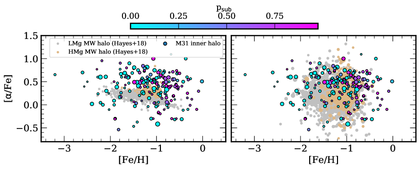
In contrast to earlier work (using DR12) on metal-poor MW field stars (Hawkins et al., 2015) that relied on kinematical selection, Hayes et al. (2018) used a larger sample of stars in combination with a data-driven approach to identify stellar populations that were distinct in multi-dimensional chemical abundance space. This resulted in the identification of two kinematically and chemically distinct MW stellar halo populations characterized by low-[Mg/Fe] with negligible Galactic rotation (LMg) and high-[Mg/Fe] with significant Galactic rotation (HMg). Based on these chemodynamical properties, Hayes et al. concluded that the origin of the LMg population is likely massive progenitors similar to the Large Magellanic Cloud (LMC; $M_{\star}\sim 10^{9.5}M_{\odot}$), accreted early in the MW’s history (i.e., Gaia-Enceladus; Haywood et al. 2018). The HMg population was likely formed in-situ, either via dissipative collapse or disk heating. In a companion study, Fernández-Alvar et al. (2018) modeled the chemical evolution of the two populations to find that HMg stars experienced a more intense and long-lived star formation history than LMg stars .

Figure 11 presents a comparison between [$\alpha$/Fe] and [Fe/H] for 1,321 stars from the metal-poor halo ([Fe/H] $<$ $-$0.9) sample of Hayes et al. (2018) and 197 RGB stars in the inner stellar halo of M31 (Escala et al. 2019, 2020; Gilbert et al. 2019; this work). The atmospheric [$\alpha$/Fe] from Hayes et al. (2018) is measured from spectral synthesis by the APOGEE Stellar Parameters and Chemical Abundances Pipeline (ASPCAP; García Pérez et al. 2016) based on a fit to all $\alpha$-elments (O, Mg, Si, Ca, S, and Ti; Holtzman et al. 2015) in the infrared H-band ($1.514-1.696$ $\mu$m). We show both the LMg and HMg populations for the MW, whereas M31’s inner halo stellar population is color-coded according to kinematically-based substructure probability.

Although the abundance distributions of the MW and M31 halo stars clearly overlap, the spread in [$\alpha$/Fe] (and perhaps [Fe/H]) for the M31 RGB stars is much larger owing to the uncertainties on our measurements. The typical measurement uncertainties for M31 RGB stars are $\delta_{\textrm{[Fe/H]}}\sim 0.12$ and $\delta_{\textrm{[$\alpha$/Fe]}}\sim 0.30$, compared to $\sim$0.04 for MW halo stars in the Hayes et al. (2018) sample. In order to perform a more direct comparison between M31’s and the MW’s chemical abundance distributions, we perturbed the MW halo abundances by uncertainties from 10⁴ draws of the empirical error distribution of our measurements. During each draw, each MW halo star was perturbed by random values sourced from a normal distribution defined by the uncertainties on a single randomly selected M31 RGB star and the MW halo star. The M31 RGB star is randomly selected from a metallicity bin within 0.2 dex of the MW halo star to preserve the metallicity-dependence of the M31 error distribution: M31 RGB stars with lower [Fe/H] tend to have larger [Fe/H] uncertainties.

We show an example of a single perturbation of the MW halo stars in the upper right panel of Figure 11. The primary effect of this perturbation is that the MW halo stars now span a similar range in [$\alpha$/Fe] as the M31 halo stars. .

By performing the above exercise, we constructed empirical PDFs in [$\alpha$/Fe] vs. [Fe/H] space for the LMg and HMg populations (Figure 12). In this figure, we qualitatively compared M31 RGB stars that likely belong to M31’s dSph-like population ($p_{\rm dSph}$ $>$ 0.75; Eq. 15) to the MW PDFs. A subset of M31’s dSph-like stars appear similar to the LMg population, but it is unclear if all of M31’s dSph-like stars could originate from a LMg-like population. In particular, M31’s halo may have stars that are more metal-poor ([Fe/H] $\lesssim$ $-$1.8) than those observed in Hayes et al.’s MW halo sample. We note that the APOGEE abundances attributed to Gaia-Enceladus from Helmi et al. (2018) extend down to [Fe/H] $\sim$ $-$2.5 and up to [$\alpha$/Fe] $\sim$ 0.5, potentially encapsulating the low-metallicity RGB stars in M31’s dSph-like population.

Figure 12: Empirical PDFs for the LMg (grey solid lines) and HMg (dashed brown lines) populations of the MW halo (Hayes et al., 2018), computed from 10⁴ perturbations of the MW abundances by M31’s measurement errors (§ 6.1). The contour levels correspond to 16^th, 50^th, and 84^th percentiles. We also show RGB stars in the smooth halo of M31 with dSph-like chemical abundances (§ 5.4.2) as colored points. A subset of the dSph-like stars appears similar to the LMg population, but it is unclear if all of such stars could originate from a LMg-like population.

Figure 13: [$\alpha$/Fe] versus [Fe/H] for RGB stars in the inner halo of M31 compared to the Magellanic Clouds (black points; Nidever et al. 2019; § 6.2): the SMC (left) and LMC (right). The point scaling for the M31 data is the same as in Figure 10. We do not show the small measurement uncertainties for the MCs ($\delta_{\rm[Fe/H]}\sim 0.02$, $\delta_{\rm[\alpha/Fe]}\sim 0.03$).

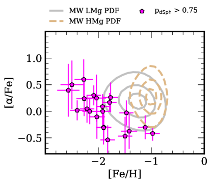
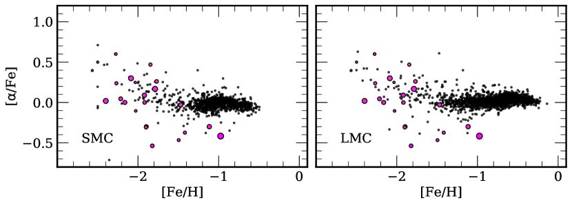
6.1.1 Potential Sources of Systematic Offsets

We refrained from drawing detailed conclusions based on these comparisons owing to potential systematic offsets in the abundance distributions between the MW and M31 data sets. As previously discussed, the APOGEE chemical abundances are based on high-resolution spectroscopy in the near-infrared H-band, in contrast with our measurements, which we derive from low- ($R\sim 3000$) and medium- ($R\sim 6000$) resolution spectroscopy at optical wavelengths with comparatively low S/N. Additionally, the APOGEE abundances are internally calibrated against observations of metal-rich open clusters (Holtzman et al., 2015) and externally calibrated to correct for systematic offsets. Although our spectral synthesis method relies on MW globular clusters to determine the systematic uncertainty on our abundance measurements (Kirby et al., 2008; Escala et al., 2019, 2020), we do not calibrate the stellar parameters and elemental abundances outputted by our abundance pipelines to external observations. The selection functions also differ between Hayes et al. (2018) and this work, where we have avoided selection criteria based on chemical abundances. Although we acknowledge these caveats, an exploration of the impact of these possible systematic offsets and selection effects between the MW and M31 data sets is beyond the scope of this paper.

6.2 Comparison of M31’s dSph-like Stars to the Magellanic Clouds

we compared the abundances of M31’s to the Magellanic Clouds (MCs), which have stellar masses ($2.7\times 10^{9}$ $M_{\odot}$ and $3.1\times 10^{8}$ $M_{\odot}$ for the LMC and SMC, respectively; van der Marel et al. 2002; Stanimirović et al. 2004) We used the MC abundance sample of Nidever et al. (2019) from APOGEE DR16 (Ahumada et al., 2019) obtained as part of SDSS-IV (Blanton et al., 2017) through the installation of a second APOGEE spectrograph in the Southern hemisphere (Wilson et al., 2019). Figure 13 shows [$\alpha$/Fe] versus [Fe/H] for the MC samples compared to M31’s dSph-like stars. The MCs show the same broad chemical abundance trends defined by low [$\alpha$/Fe], a relatively metal-rich body, and a metal-poor tail extending to higher [$\alpha$/Fe]. Figure 13 further illustrates that M31 RGB stars with $p_{\rm dSph}>$ 0.75 and the metal-poor, high-$\alpha$ tails of the MCs

Chemical evolution models for the LMC predict the dominance of Type Ia supernovae over core-collapse supernovae during this quiescent epoch (Bekki & Tsujimoto, 2012; Nidever et al., 2019), resulting in the observed decline in [$\alpha$/Fe] with [Fe/H] in the metal-poor tails. the predicted age-metallicity relation from Nidever et al. (2019) has the LMC reaching [Fe/H]$\sim-1.5$ at 6 Gyr into its evolution (Nidever et al., 2019), suggesting that the majority of its metal-poor tail was in place by $\sim$7 Gyr ago.

Based on their chemical abundances, Nidever et al. (2019) concluded that the early evolution of the MCs was characterized by low star formation efficiency (gas mass converted into stellar mass). This low efficiency may result from the MCs having evolved in isolation, given that they are likely on first infall into the MW’s potential well (Besla et al., 2007, 2012). The relatively quiescent star formation history of the MCs until $\sim$4 Gyr ago may be a consequence of such isolation (e.g., Smecker-Hane et al. 2002; Harris & Zaritsky 2009; Weisz et al. 2013).

Thus, we can infer that the galaxie(s) that were accreted to form its dSph-like population, which is characterized by low star formation efficiency, . We evaluate whether the scenario of multiple low-mass progenitors (LM-SFH) or a dominant high-mass progenitor (HM-SFE) is more likely to explain the origin of M31’s dSph-like stars in § 6.3.2.

6.3 Formation Scenarios for M31’s Inner Stellar Halo

In this subsection, we explore the implications of our abundance measurements in M31’s stellar halo for in-situ and accreted formation channels (§ 6.3.1). We also investigate possible origins of M31’s dSph-like population in the context of the stellar mass function of accreted galaxies (§ 6.3.2).

6.3.1 The In-Situ vs. Accreted Halo

Simulations predict the existence of an in-situ component of the stellar halo, which formed in the main progenitor of the host galaxy, in addition to an accreted component formed from external galaxies (Zolotov et al., 2009; Font et al., 2011; Tissera et al., 2013; Cooper et al., 2015). In addition to a component formed via dissipative collapse, the in-situ halo includes contributions from kinematically heated stars originating in the disk (Purcell et al., 2010; McCarthy et al., 2012; Tissera et al., 2013; Cooper et al., 2015). The relative contributions of these two formation channels to stellar halo build-up depend on the stochastic accretion history of the host galaxy, where more active histories correspond to lower in-situ stellar halo mass fractions (Zolotov et al., 2009). However, the in-situ fraction also depends on the numerical details of a given simulation (Zolotov et al., 2009; Cooper et al., 2015). The more recent simulations of Cooper et al. (2015) have found that the in-situ fraction typically ranges between $\sim$30-40%. Despite variations in the predictions of this fraction, multiple studies have found that the in-situ component tends to dominate within the inner $\sim$20-30 kpc of the stellar halo (Zolotov et al., 2009; Font et al., 2011; Tissera et al., 2013; Cooper et al., 2015).

Predicted chemical signatures for the in-situ and accreted stellar halo can also vary depending on the simulation. In some studies (Zolotov et al., 2009; Font et al., 2011; Tissera et al., 2013, 2014), in-situ star formation produces more metal-rich stellar halos than accretion alone. In contrast, Cooper et al. (2015) argued that the in-situ and accreted halo may be indistinguishable based on metallicity alone, assuming that the in-situ halo forms mostly from gas stripped from accreted galaxies. For galaxies that have not experienced a recent ($z\lesssim 1$) major merger, Zolotov et al. (2010) found that the in-situ halo has higher [$\alpha$/Fe] at fixed [Fe/H] than the accreted halo for stars with [Fe/H] $>-1$ in the solar neighborhood. Tissera et al. (2012, 2013) found the opposite trend, where accreted stars tend to be more $\alpha$-enhanced (but also more metal-poor) than in-situ stars.

On the observational front, a bimodality in the metallicity of the MW’s stellar halo with radius was interpreted as evidence in favor of a two-component halo defined by in-situ and accreted populations (Carollo et al., 2007, 2010). After Gaia DR2, it has become apparent that the MW’s presumably in-situ inner stellar halo is in actuality the remnants of Gaia-Enceladus (Helmi et al., 2018; Haywood et al., 2018; Belokurov et al., 2018; Deason et al., 2018). A veritable in-situ component of the inner stellar halo has recently emerged via its distinct chemical composition and kinematics in relation to Gaia-Enceladus tidal debris (Hayes et al. 2018; Haywood et al. 2018; Di Matteo et al. 2019; Gallart et al. 2019; Conroy et al. 2019, with earlier suggestions from Gaia DR1 by Bonaca et al. 2017). In particular, Belokurov et al. (2020) identified this component from old, high-eccentricity, $\alpha$-rich stars on retrograde orbits where with ${\rm[Fe/H]}>-0.7$ in the solar neighborhood, associating it with formation from the MW’s proto-disk following its last significant merger.

At this time, the presence of a significant in-situ component in the inner stellar halo of M31 is less clear than in the case of the MW. Along the major axis of M31’s northeastern disk, there is compelling kinematical evidence for both a rotating inner spheroid (Dorman et al., 2012) and dynamically heated stars originating from the disk (Dorman et al., 2013). An extended disk-like structure possibly formed from M31’s last significant merger has also been detected within the inner $\sim$40 kpc of M31’s disk plane (Ibata et al., 2005). Although these stellar structures may reasonably be various in-situ components, they have not been detected within the radial range spanned by our data ($\sim$8-34 kpc in M31’s southeastern quadrant, along its minor axis; Figure 1). Even at the distance of our innermost spectroscopic field ($r_{\rm proj}\sim 9$ kpc, or $r_{\rm disk}\sim$ 38 kpc assuming $i=77^{\circ}$), the contribution from the extended disk is expected to be $\lesssim$10% (Guhathakurta et al., 2005; Gilbert et al., 2007).

Interestingly, M31’s global stellar halo properties appear to agree with predictions from accretion-only models for stellar halo formation (Harmsen et al., 2017), along with other MW-like, edge-on galaxies in the Local Volume from the GHOSTS survey (Radburn-Smith et al., 2011; Monachesi et al., 2016a). Indeed, multiple lines of evidence indicate that accretion has played a dominant role in the formation of M31’s stellar halo (§ 6.3.2).

Based on this alone, both the dSph-like and non-dSph-like stars in M31’s smooth, inner stellar halo (§ 5.4.2) could be accreted populations resulting from chemically distinct groups of progenitors. the similarity of their chemical abundance patterns to M31’s dSphs provides strong evidence in favor of an accretion origin .

Conversely , the overlap between M31’s broader stellar halo population and the MW’s in-situ HMg population in abundance space (§ 6.1; Figure 11) suggests that M31 could reasonably possess a ancient in-situ population, instead of having a accretion origin in distinct progenitor(s). In an in-situ formation scenario, the bulk of M31’s metal-rich stars in the smooth halo may have originated from a proto-stellar disk, similar to the MW’s in-situ halo population (Belokurov et al., 2020). Given that we are lacking multi-dimensional kinematical information or higher-dimensional chemical information, it is difficult to distinguish between accreted and in-situ formation scenarios for the bulk of M31’s stellar population without performing a detailed comparison to simulations, which is beyond the scope of this paper.

6.3.2 The Mass Function of Destroyed Galaxies

The general consensus from simulations of MW-like galaxies is that massive dwarf galaxies ($M_{\star}\sim 10^{8-10}M_{\odot}$) distinct from present-day satellites are the dominant progenitors of the accreted stellar halo (Bullock & Johnston, 2005; Robertson et al., 2005; Font et al., 2006b; Cooper et al., 2010; Deason et al., 2016; D’Souza & Bell, 2018a; Fattahi et al., 2020). These galaxies have a median accretion time of $\gtrsim$9 Gyr ago (Bullock & Johnston, 2005; Font et al., 2006b; Fattahi et al., 2020). Furthermore, a few massive progenitors are predicted to form the bulk of the accreted halo (Cooper et al., 2010; Deason et al., 2016; D’Souza & Bell, 2018a; Fattahi et al., 2020), where the secondary progenitor is on average half as massive as the primary progenitor (D’Souza & Bell, 2018a). In particular, Fattahi et al. (2020) found that such massive progenitors dominate the stellar mass budget within the inner 50 kpc of the stellar halo, where contributions from progenitors with $M_{\star}<10^{8}M_{\odot}$ become non-negligible around $\sim$100 kpc.

The details of the stellar mass function of destroyed constituent galaxies are dictated by the accretion history of the host galaxy. Deason et al. (2016) found that MW-like galaxies with more active accretion histories have higher mass accreted progenitors ($M_{\star}\sim 10^{9-10}M_{\odot}$) and larger accreted halo mass fractions than their quiescent counterparts. The wealth of substructure visible in M31’s stellar halo (e.g., Ferguson et al. 2002; Ibata et al. 2007; McConnachie et al. 2018), including the GSS (Ibata et al., 2001), and the lack of an apparent break in its density profile (Guhathakurta et al., 2005; Irwin et al., 2005; Courteau et al., 2011; Gilbert et al., 2012) suggests that M31 has likely experienced multiple and continuous contributions to its stellar halo from accreted galaxies (Deason et al., 2013; Cooper et al., 2013; Font et al., 2020). Moreover, the total accreted stellar mass of M31 ($1.5\pm 0.5\times 10^{10}M_{\odot}$; Harmsen et al. 2017) is on the upper end of both observed (Merritt et al., 2016; Harmsen et al., 2017) and predicted (Cooper et al., 2013; Deason et al., 2016; Monachesi et al., 2019) accreted stellar halo mass fractions for MW-like galaxies.

The large-scale negative metallicity gradient of M31’s stellar halo (Gilbert et al. 2014, 2020; this work) may also lend support to it being dominated by a few massive progenitors, although this trend could also result from a significant in-situ component in the inner regions of the halo (Font et al., 2011; Tissera et al., 2014; Monachesi et al., 2019). Thus, M31’s accreted mass function is likely weighted toward progenitor galaxies with $M_{\star}\sim 10^{9-10}M_{\odot}$. This agrees with the hypothesis that the main contributor to M31’s stellar halo (including substructure) is the GSS progenitor, a massive galaxy with $M_{\star}\sim 10^{9-10}M_{\odot}$ accreted between $\sim$1-4 Gyr ago, depending on the merger scenario (Fardal et al., 2007, 2008; Hammer et al., 2018; D’Souza & Bell, 2018b).

The mass spectrum of progenitor galaxies dictates the metallicity of the accreted stellar halo through the stellar mass-metallicity relation for galaxies (Gallazzi et al., 2005; Kirby et al., 2013) and its redshift evolution (Gallazzi et al., 2014; Ma et al., 2016; Leethochawalit et al., 2018, 2019). In particular, Leethochawalit et al. (2018, 2019) found that the normalization of the stellar-mass metallicity relation evolves by 0.04 $\pm$ 0.01 dex Gyr^-1. Assuming that this relation extends to $M_{\star}<10^{9}\ M_{\odot}$, this means that an SMC-mass galaxy ($M_{\star}\sim 10^{8.5}\ M_{\odot}$) accreted 10 Gyr ago would have $\langle$[Fe/H]$\rangle=-1.39\pm 0.04$, compared to $\langle$[Fe/H]$\rangle=-0.99\pm 0.01$ at $z=0$ (Nidever et al., 2019). Observations of the MW-like GHOSTS galaxies (Harmsen et al., 2017) have firmly established such a relationship between stellar halo mass and metallicity, as first suggested by Mouhcine et al. (2005). The physical driving force for this relation is the fact that the most massive progenitors dominate halo assembly (D’Souza & Bell, 2018a; Monachesi et al., 2019).

In addition to setting the stellar halo metallicity, the most massive progenitors largely determine the full metallicity distribution function of the stellar halo (Deason et al., 2016; Fattahi et al., 2020). For a typical progenitor mass of 10^9-10 $M_{\odot}$, these galaxies contribute $\gtrsim$90% of metal-poor stars ([Fe/H] $<$ $-$1) and $\sim$20-60% of stars with [Fe/H] $<$ $-2$ (Deason et al., 2016). Deason et al. also found that classical dwarf galaxies ($M_{\star}\sim 10^{5-8}M_{\odot}$) contribute the remainder of metal-poor stars, with negligible contributions from ultra-faint dwarf galaxies.

Indeed, M31’s dSph-like stars most likely have an accretion origin owing to their defining similarity to the abundance patterns M31 dwarf galaxies (§ 5.4.2). Given that (1) the chemical abundance patterns of M31’s dSph-like population are broadly consistent with the low-metallicity ([Fe/H] $\lesssim-1.5$), early evolution of the MCs (§ 6.2) and (2) we do not detect any kinematical substructure for this population (§ 5.4), the accreted galaxies(s) that contributed to M31’s dSph-like population could have been massive ($M_{\star}\sim 10^{8-9}M_{\odot}$) if they evolved in an isolated, low star formation efficiency environment and were accreted $\gtrsim$ 8 Gyr ago.

Given M31’s halo properties and inferred accretion history (based on halo formation models), a possible scenario for the formation of the dSph-like population ($-2.5\lesssim$ [Fe/H] $\lesssim-1.0$) is the accretion of a massive, secondary progenitor . Assuming that the GSS progenitor is the dominant progenitor, the stellar mass of this secondary progenitor should be approximately between the mass of the SMC and LMC ($M_{\star}\sim 10^{8.5-9.5}M_{\odot}$; § 6.2) and possibly comparable to Gaia-Enceladus (§ 6.1). An early, massive accretion event such as this would also deposit its debris closer to the center of the host potential in the inner halo owing to dynamical friction (Cooper et al., 2010; Tissera et al., 2013; Fattahi et al., 2020). Alternatively, M31’s dSph-like population could have formed exclusively from the accretion of multiple progenitors similar to classical dwarf galaxies . Although this hypothesis cannot be rejected, it is less favored by the predictions of stellar halo formation in a cosmological context (Bullock & Johnston, 2005; Font et al., 2006b; Deason et al., 2016; D’Souza & Bell, 2018a).

To discern between the LM-SFH and HM-SFE hypotheses, we consider the accretion of an SMC-mass galaxy onto M31 $\sim$10 Gyr ago. Assuming a significant metallicity dispersion as observed in LG galaxies ($\sim$0.4 dex; e.g., Kirby et al. 2013; Ho et al. 2015; Kirby et al. 2020), such a galaxy would span $-1.9\ (-2.2)\lesssim\langle{\rm[Fe/H]}\rangle\lesssim-0.9\ (-0.6)$ within 1$\sigma$ (2$\sigma$). It is unclear if such a galaxy could account for the most metal-poor stars observed in M31’s dSph-like population ([Fe/H] $\lesssim$ $-2.2$). Additional progenitors with $M_{\star}\sim 10^{7-8}\ M_{\odot}$ may be necessary to explain these low-metallicity stars

7 Summary

We have presented measurements of [$\alpha$/Fe] and [Fe/H] for 128 individual M31 RGB stars from low- ($R\sim 3000$) and medium- ($R\sim 6000$) resolution Keck/DEIMOS spectroscopy. With a combined sample of 197 M31 RGB stars with abundance measurements in inner halo fields (Escala et al. 2019, 2020; Gilbert et al. 2019; this work), we have undertaken an analysis of the chemical abundance properties of M31’s kinematically smooth stellar halo between 8–34 kpc. Our primary results are the following:

1. We measured $\langle$[Fe/H]$\rangle$ = $-$1.08 $\pm$ 0.04 ($-$1.17 $\pm$ 0.04) and $\langle$[$\alpha$/Fe]$\rangle$ = 0.40 $\pm$ 0.03 (0.39 $\pm$ 0.03) including (excluding) substructure in M31’s inner stellar halo (§ 5.3).

2. We measured a radial [Fe/H] gradient of $-$0.025 $\pm$ 0.002 dex kpc^-1, with an intercept of [Fe/H] = $-$0.72 $\pm$ 0.03, for the smooth halo (§ 5.3). Including substructure results in a shallower [Fe/H] gradient ($-$0.018 $\pm$ 0.001). We did not find statistically significant radial gradients in [$\alpha$/Fe], including or excluding substructure.

3. We reaffirmed previous results based on smaller sample sizes (Escala et al., 2020; Kirby et al., 2020) that the chemical abundance distribution of M31’s inner halo is incompatible with having formed from progenitors similar to present-day M31 dSphs (Vargas et al., 2014a; Kirby et al., 2020) when taken as a whole (§ 5.4.1).

4. we robustly identified a subset of stars ($N$ = 22 with $p_{\rm dSph}>$ 0.75; Eq. 15) belonging to smooth halo that have [Fe/H] and [$\alpha$/Fe] measurements consistent with M31 dSphs (§ 5.4.2).

5. We compared the abundance distributions of the stellar halos of M31 and the MW (Hayes et al. 2018; § 6.1), finding that M31’s halo appears to be more metal-rich and $\alpha$-rich on average.

6. We compared M31’s dSph-like stars to the Magellanic Clouds (Nidever et al., 2019), finding that the population’s chemical evolution is similar to that of the MCs at [Fe/H] $\lesssim-1.5$ (§ 6.2). This indicates that the dSph-like stars could have formed in an environment, , resulting in low star formation efficiency.

7. We concluded that M31’s dSph-like population was likely accreted (§ 6.3) . The remaining, dominant population of stars in the smooth component of M31’s halo may result from progenitor(s) distinct from those of the dSph-like population, or represent an in-situ stellar halo component.

Appendix A Catalog of Stellar Parameters and Abundances

Stellar parameters and elemental abundances of individual M31 RGB stars for fields f109_1, f123_1, f130_1, a0_1, and a3 are presented in Table 4. The table includes data for 128 total M31 RGB stars with reliable [Fe/H] and [$\alpha$/Fe] measurements (§ 5.1), in addition to 80 M31 RGB stars that only have reliable [Fe/H] measurements.

Table 4: Stellar Parameters and Elemental Abundances of Individual M31 RGB Stars

Object	Sky Coordinates		$v_{\rm{helio}}$	S/N	$T_{\rm eff}$	$\delta(T_{\rm eff}$)	$\log$ $g$	[Fe/H]	$\delta$([Fe/H])	[$\alpha$/Fe]	$\delta$([$\alpha$/Fe])
ID	RA	Dec	(km s-1)	(Å -1)	(K)	(K)	(dex)	(dex)	(dex)	(dex)	(dex)
f109_1 (9 kpc Halo Field)
1092408	00h45m44.35s	+40∘54${}^{{}^{\prime}}$15.0${}^{{}^{\prime\prime}}$	$-$281.6	15	3883	5	0.64	$-$0.96	0.13	0.23	0.27
1095375	00h45m49.45s	+40∘58${}^{{}^{\prime}}$53.8${}^{{}^{\prime\prime}}$	$-$190.4	12	4082	10	1.06	$-$0.83	0.14	0.39	0.38
1092785	00h45m44.27s	+40∘54${}^{{}^{\prime}}$52.2${}^{{}^{\prime\prime}}$	$-$288.9	13	3975	6	0.77	$-$0.56	0.13	0.68	0.26
f123_1 (18 kpc Halo Field)
1230048	00h48m18.89s	+40∘20${}^{{}^{\prime}}$18.1${}^{{}^{\prime\prime}}$	$-$350.2	7	4825	51	1.51	$-$0.81	0.17	$\cdots$	$\cdots$
1230053	00h48m05.10s	+40∘20${}^{{}^{\prime}}$22.8${}^{{}^{\prime\prime}}$	$-$158.2	22	4554	41	0.73	$-$1.92	0.12	0.09	0.23
1230079	00h48m18.52s	+40∘20${}^{{}^{\prime}}$40.1${}^{{}^{\prime\prime}}$	$-$324.3	13	4198	39	0.91	$-$1.00	0.11	0.58	0.24
f130_1 (23 kpc Halo Field)
1300360	00h49m12.01s	+40∘10${}^{{}^{\prime}}$00.3${}^{{}^{\prime\prime}}$	$-$280.2	14	3938	8	1.14	$-$1.15	0.14	0.56	0.25
1300698	00h49m03.01s	+40∘15${}^{{}^{\prime}}$05.1${}^{{}^{\prime\prime}}$	$-$235.4	15	3774	37	0.98	$-$0.34	0.14	0.60	0.29
1300024	00h49m06.69s	+40∘04${}^{{}^{\prime}}$54.2${}^{{}^{\prime\prime}}$	$-$360.4	52	4459	3	0.66	$-$2.60	0.16	0.70	0.23
a0_1 (31 kpc Halo Field)
8002454	00h51m59.62s	+39∘46${}^{{}^{\prime}}$49.7${}^{{}^{\prime\prime}}$	$-$317.4	11	3991	14	1.19	$-$1.18	0.14	$\cdots$	$\cdots$
7007191	00h51m30.89s	+39∘55${}^{{}^{\prime}}$56.4${}^{{}^{\prime\prime}}$	$-$278.1	19	4410	14	1.13	$-$1.55	0.15	0.10	0.43
7003904	00h51m49.68s	+39∘51${}^{{}^{\prime}}$43.1${}^{{}^{\prime\prime}}$	$-$268.2	21	3991	11	0.80	$-$1.19	0.13	0.38	0.32
a3_1 (33 kpc Halo Field)
7003496	00h03m12.68s	+39∘00${}^{{}^{\prime}}$28.1${}^{{}^{\prime\prime}}$	$-$278.5	11	4261	34	1.31	$-$2.90	0.26	$\cdots$	$\cdots$
7003469	00h03m12.76s	+39∘03${}^{{}^{\prime}}$16.7${}^{{}^{\prime\prime}}$	$-$462.2	9	3996	14	1.14	$-$0.56	0.14	0.74	0.33
7004205	00h03m11.44s	+38∘59${}^{{}^{\prime}}$44.0${}^{{}^{\prime\prime}}$	$-$355.3	11	3793	9	0.83	$-$1.42	0.15	$-$0.37	0.33
a3_2 (33 kpc Halo Field)
6004645	00h03m11.76s	+39∘12${}^{{}^{\prime}}$03.3${}^{{}^{\prime\prime}}$	$-$431.1	18	4372	10	0.98	$-$0.92	0.13	$-$0.19	0.35
6004424	00h03m12.05s	+39∘10${}^{{}^{\prime}}$33.0${}^{{}^{\prime\prime}}$	$-$343.6	48	4314	5	0.64	$-$2.10	0.14	0.61	0.90
7005249	00h03m11.68s	+39∘03${}^{{}^{\prime}}$36.6${}^{{}^{\prime\prime}}$	$-$412.5	19	4126	9	1.03	$-$0.77	0.13	0.06	0.18

Note. — (This table is available in its entirety in machine-readable form.).

Appendix B Identifying Probable Accreted Stars in the Stellar Halo of the MW

Figure 14: (Left panel) The perturbed abundance distributions of the MW halo (Hayes et al., 2018), separated into LMg (grey points) and HMg (brown points) populations, and the SMC MP tail (black points; Nidever et al. 2019). The 2D PDFs fitted to the entire MW halo and the SMC MP tail are shown as yellow and magenta contours, respectively. (Middle panel) The 2D PDFs fitted to the perturbed abundance distributions compared against the unperturbed abundance distributions. (Right panel) The unperturbed MW halo abundance distribution color-coded according to a star’s probability of being SMC-like (defined analogously to Eq. 15), as evaluated from the perturbed abundance distributions. Magenta stars are SMC-like, whereas yellow stars are not.

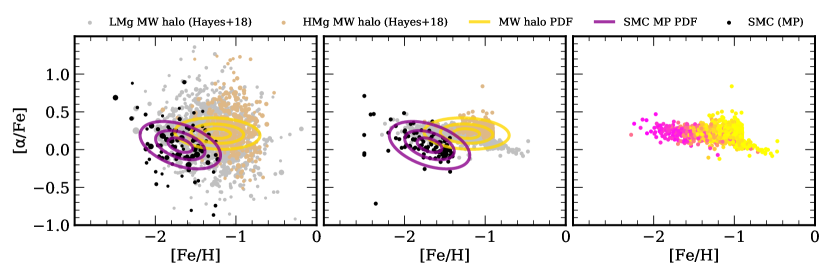
In § 5.4.2, we modeled the 2-D chemical abundance distributions of M31’s stellar halo and its dSphs in order to statistically identify M31 RGB stars with abundances similar to M31 dSphs. The suggestion that such stars may exist in M31’s stellar halo was first made apparent by Figure 9 through a comparison to abundance measurements in M31 dSphs obtained using the same techniques. In this Appendix, we use APOGEE chemical abundances of the MW’s stellar halo (Hayes et al., 2018) and the ancient, metal-poor tail of the SMC (§ 6.2; Nidever et al. 2019), which we perturb by an M31-like error distribution (§ 6.1), to illustrate the efficacy of this method for successfully recovering dwarf-galaxy-like stars in a stellar halo population.

Figure 14 outlines the steps in this proof of concept. First, we perturbed the MW’s halo abundance distribution by M31-like errors, as described in § 6.1. Then, we fit a 2D PDF, following § 5.4.2, to the perturbed MW halo abundances without separating it into the LMg or HMg populations of Hayes et al. 2018. The left panel of Figure 14 illustrates the resulting PDF (yellow contours). Next, we isolated the metal-poor tail of the SMC abundance distribution ([Fe/H] $\lesssim-1.4$). As discussed in § 6.2, chemical evolution models for the Large Magellanic Cloud (Bekki & Tsujimoto, 2012; Nidever et al., 2019) indicate that its metal poor tail was in place by $\sim$7-9 Gyr ago at the latest. Given the similarly low star formation efficiency of the SMC (Nidever et al., 2019), we can assume that its metal-poor tail is similarly ancient. The more ancient, metal-poor portion of the SMC abundance distribution is the relevant portion to compare to the predominately old stellar halo of the MW (e.g., Gallart et al. 2019; Bonaca et al. 2020). We perturbed the SMC metal-poor tail by M31-like errors and fit a 2D PDF to resulting abundance distribution (left panel of Figure 14, magenta contours).

The middle panel of Figure 14 shows the original unperturbed MW halo and SMC abundance distributions compared to the 2D PDFs calculated from the perturbed distributions. We used the MW halo PDF and the SMC metal-poor (MP) PDF to calculate a probability that each MW halo star has abundances similar to the SMC (analogously to Eq. 15). To calculate this probability, we used the perturbed values of the abundances for a given star. The right panel of Figure 14 shows the unperturbed MW halo abundances color-coded according to this probability calculated using the perturbed equivalent.

Figure 15: Stars identified as SMC-like ($p_{\rm SMC}>$ 0.75; pink circles) compared to MW halo stars that were not classified as SMC-like separated according their membership in the LMg or HMg population (black and brown points, respectively; Hayes et al. 2018). Some stars classified as SMC-like reside close to the HMg region of the MW halo abundance distribution because they were classified based on their perturbed abundances and uncertainties. 99% of SMC-like stars are correctly classified as originating from the accreted LMg population. (Right panel) 2D PDFs fit to abundance distributions of the perturbed MW halo (solid yellow contours) and SMC MP tail (solid pink contours), compared to 2D PDFs fit to the unperturbed equivalents (dashed gold and purple contours, respectively). The true, underlying abundance distribution is constrained by both the perturbed and unperturbed abundance distributions.

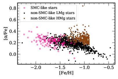
We compared the stars classified as “SMC-like” ($p_{\rm SMC}>$ 0.75) by the perturbation analysis to the stars that are truly SMC-like (e.g., the LMg stars). The LMg population corresponds to stars that were accreted during the Gaia-Enceladus merger event (§ 6.1; Helmi et al. 2018; Belokurov et al. 2018; Haywood et al. 2018) of a galaxy at least as massive as the SMC. Assuming that stars with $p_{\rm SMC}>0.75$ (0.5) are SMC-like, this results in the correct classification of 99% (98%) of SMC-like stars as belonging to the LMg population. If we assume that stars with $p_{\rm SMC}<0.25$ (0.5) are not SMC-like, this results in the correct classification of 38% (32%) of not-SMC-like stars as belonging to the HMg population. This is because the classification of SMC-like stars is incomplete at high metallicity beyond the bounds of the SMC MP PDF. However, the relevant point for our analysis is that the classification of stars as SMC-like is highly accurate. Repeating this exercise for different perturbations of the MW halo and SMC abundance distributions does not alter these percentages by more than 0.5%.

Figure 15 further supports this analysis. The left panel shows stars that we have identified as SMC-like overlaid on the full MW halo abundance distribution, where it is evident that the overwhelming majority of SMC-like stars correspond to the LMg population. The right panel shows PDFs fit to the perturbed and unperturbed abundance distributions for the MW halo and SMC MP tail. The primary difference between the perturbed and unperturbed PDFs is that the unperturbed PDFs are narrower in the [$\alpha$/Fe] direction, whereas the shapes, angles, and metallicity spreads between each case are similar. Both the perturbed and unperturbed distributions represent approximations of the true, underlying parent distribution. The fact that they show significant overlap demonstrates that we can in fact reasonably constrain the underlying PDFs describing the abundance distributions in spite of our uncertainties in [$\alpha$/Fe].

In this example, the statistical methodology developed in § 5.4.2 is successful at identifying MW stars that are similar in their 2D [$\alpha$/Fe] vs. [Fe/H] abundances to stars in the metal-poor tail of the SMC abundance distribution, using abundances perturbed by the typical uncertainties in our M31 sample. This gives us confidence that we can statistically identify M31 halo stars that are similar in their 2D [$\alpha$/Fe] vs. [Fe/H] abundances to stars in M31’s dSph galaxies, and thus may have formed in similar environments and been accreted onto M31’s halo. This is true despite the fact that we did not assume any knowledge about the true underlying abundance distributions, and despite the size of the uncertainties [$\alpha$/Fe]. Thus, this statistical method can successfully identify dwarf-galaxy-like stars not only in the MW’s halo, but also in the smooth component of M31’s stellar halo.

References

- Albareti et al. (2017) Albareti, F. D., Allende Prieto, C., Almeida, A., et al. 2017, ApJS, 233, 25
- Ahumada et al. (2019) Ahumada, R., Allende Prieto, C., Almeida, A., et al. 2019, arXiv e-prints, arXiv:1912.02905
- Astropy Collaboration et al. (2013) Astropy Collaboration, Robitaille, T. P., Tollerud, E. J., et al. 2013, A&A, 558, A33
- Astropy Collaboration et al. (2018) Astropy Collaboration, Price-Whelan, A. M., Sipőcz, B. M., et al. 2018, AJ, 156, 123
- Bekki & Tsujimoto (2012) Bekki, K., & Tsujimoto, T. 2012, ApJ, 761, 180
- Belokurov et al. (2018) Belokurov, V., Erkal, D., Evans, N. W., et al. 2018, MNRAS, 478, 611
- Belokurov et al. (2020) Belokurov, V., Sanders, J. L., Fattahi, A., et al. 2020, MNRAS, doi:10.1093/mnras/staa876
- Besla et al. (2007) Besla, G., Kallivayalil, N., Hernquist, L., et al. 2007, ApJ, 668, 949
- Besla et al. (2012) Besla, G., Kallivayalil, N., Hernquist, L., et al. 2012, MNRAS, 421, 2109
- Blanton et al. (2017) Blanton, M. R., Bershady, M. A., Abolfathi, B., et al. 2017, AJ, 154, 28
- Bonaca et al. (2017) Bonaca, A., Conroy, C., Wetzel, A., et al. 2017, ApJ, 845, 101
- Bonaca et al. (2020) Bonaca, A., Conroy, C., Cargile, P. A., et al. 2020, arXiv e-prints, arXiv:2004.11384
- Brown et al. (2007) Brown, T. M., Smith, E., Ferguson, H. C., et al. 2007, ApJ, 658, L95.
- Brown et al. (2006) Brown, T. M., Smith, E., Ferguson, H. C., et al. 2006, ApJ, 652, 323.
- Brown et al. (2008) Brown, T. M., Beaton, R., Chiba, M., et al. 2008, ApJ, 685, L121
- Brown et al. (2009) Brown, T. M., Smith, E., Ferguson, H. C., et al. 2009, ApJS, 184, 152
- Bullock & Johnston (2005) Bullock, J. S., & Johnston, K. V. 2005, ApJ, 635, 931
- Carollo et al. (2007) Carollo, D., Beers, T. C., Lee, Y. S., et al. 2007, Nature, 450, 1020
- Carollo et al. (2010) Carollo, D., Beers, T. C., Chiba, M., et al. 2010, ApJ, 712, 692
- Chapman et al. (2006) Chapman, S. C., Ibata, R., Lewis, G. F., et al. 2006, ApJ, 653, 255
- Clementini et al. (2011) Clementini, G., Contreras Ramos, R., Federici, L., et al. 2011, ApJ, 743, 19
- Cohen et al. (2018) Cohen, R. E., Kalirai, J. S., Gilbert, K. M., et al. 2018, AJ, 156, 230
- Collins et al. (2011) Collins, M. L. M., Chapman, S. C., Ibata, R. A., et al. 2011, MNRAS, 413, 1548
- Conn et al. (2016) Conn, A. R., McMonigal, B., Bate, N. F., et al. 2016, MNRAS, 458, 3282
- Conroy et al. (2019) Conroy, C., Naidu, R. P., Zaritsky, D., et al. 2019, ApJ, 887, 237
- Cooper et al. (2010) Cooper, A. P., Cole, S., Frenk, C. S., et al. 2010, MNRAS, 406, 744
- Cooper et al. (2012) Cooper, M. C., Griffith, R. L., Newman, J. A., et al. 2012, MNRAS, 419, 3018
- Cooper et al. (2013) Cooper, A. P., D’Souza, R., Kauffmann, G., et al. 2013, MNRAS, 434, 3348
- Cooper et al. (2015) Cooper, A. P., Parry, O. H., Lowing, B., et al. 2015, MNRAS, 454, 3185
- Courteau et al. (2011) Courteau, S., Widrow, L. M., McDonald, M., et al. 2011, ApJ, 739, 20
- D’Souza & Bell (2018a) D’Souza, R., & Bell, E. F. 2018, MNRAS, 474, 5300
- D’Souza & Bell (2018b) D’Souza, R., & Bell, E. F. 2018, Nature Astronomy, 2, 737
- Das et al. (2020) Das, P., Hawkins, K., & Jofré, P. 2020, MNRAS, doi:10.1093/mnras/stz3537
- Deason et al. (2013) Deason, A. J., Belokurov, V., Evans, N. W., et al. 2013, ApJ, 763, 113
- Deason et al. (2016) Deason, A. J., Mao, Y.-Y., & Wechsler, R. H. 2016, ApJ, 821, 5
- Deason et al. (2018) Deason, A. J., Belokurov, V., Koposov, S. E., et al. 2018, ApJ, 862, L1
- Demarque et al. (2004) Demarque, P., Woo, J.-H., Kim, Y.-C., et al. 2004, ApJS, 155, 667
- de Vaucouleurs (1958) de Vaucouleurs, G. 1958, ApJ, 128, 465
- Di Matteo et al. (2019) Di Matteo, P., Haywood, M., Lehnert, M. D., et al. 2019, A&A, 632, A4
- Dorman et al. (2012) Dorman, C. E., Guhathakurta, P., Fardal, M. A., et al. 2012, ApJ, 752, 147
- Dorman et al. (2013) Dorman, C. E., Widrow, L. M., Guhathakurta, P., et al. 2013, ApJ, 779, 103
- Dorman et al. (2015) Dorman, C. E., Guhathakurta, P., Seth, A. C., et al. 2015, ApJ, 803, 24
- Escala et al. (2019) Escala, I., Kirby, E. N., Gilbert, K. M., et al. 2019, ApJ, 878, 42
- Escala et al. (2020) Escala, I., Gilbert, K. M., Kirby, E. N., et al. 2020, ApJ, 889, 177
- Eisenstein et al. (2011) Eisenstein, D. J., Weinberg, D. H., Agol, E., et al. 2011, AJ, 142, 72
- Faber et al. (2003) Faber, S. M., Phillips, A. C., Kibrick, R. I., et al. 2003, Instrument Design and Performance for Optical/infrared Ground-based Telescopes, 1657.
- Fardal et al. (2007) Fardal, M. A., Guhathakurta, P., Babul, A., et al. 2007, MNRAS, 380, 15.
- Fardal et al. (2008) Fardal, M. A., Babul, A., Guhathakurta, P., et al. 2008, ApJ, 682, L33
- Fattahi et al. (2019) Fattahi, A., Belokurov, V., Deason, A. J., et al. 2019, MNRAS, 484, 4471
- Fattahi et al. (2020) Fattahi, A., Deason, A. J., Frenk, C. S., et al. 2020, arXiv e-prints, arXiv:2002.12043
- Ferguson et al. (2002) Ferguson, A. M. N., Irwin, M. J., Ibata, R. A., et al. 2002, AJ, 124, 1452
- Fernández-Alvar et al. (2018) Fernández-Alvar, E., Carigi, L., Schuster, W. J., et al. 2018, ApJ, 852, 50
- Font et al. (2006b) Font, A. S., Johnston, K. V., Bullock, J. S., et al. 2006, ApJ, 638, 585
- Font et al. (2006c) Font, A. S., Johnston, K. V., Bullock, J. S., et al. 2006, ApJ, 646, 886
- Font et al. (2008) Font, A. S., Johnston, K. V., Ferguson, A. M. N., et al. 2008, ApJ, 673, 215
- Font et al. (2011) Font, A. S., McCarthy, I. G., Crain, R. A., et al. 2011, MNRAS, 416, 2802
- Font et al. (2020) Font, A. S., McCarthy, I. G., Poole-Mckenzie, R., et al. 2020, arXiv e-prints, arXiv:2004.01914
- Foreman-Mackey et al. (2013) Foreman-Mackey, D., Hogg, D. W., Lang, D., et al. 2013, PASP, 125, 306.
- García Pérez et al. (2016) García Pérez, A. E., Allende Prieto, C., Holtzman, J. A., et al. 2016, AJ, 151, 144
- Gaia Collaboration et al. (2016) Gaia Collaboration, Brown, A. G. A., Vallenari, A., et al. 2016, A&A, 595, A2
- Gaia Collaboration et al. (2018) Gaia Collaboration, Brown, A. G. A., Vallenari, A., et al. 2018, A&A, 616, A1
- Gaia Collaboration et al. (2018) Gaia Collaboration, Babusiaux, C., van Leeuwen, F., et al. 2018, A&A, 616, A10
- Gallart et al. (2019) Gallart, C., Bernard, E. J., Brook, C. B., et al. 2019, Nature Astronomy, 3, 932
- Gallazzi et al. (2005) Gallazzi, A., Charlot, S., Brinchmann, J., et al. 2005, MNRAS, 362, 41
- Gallazzi et al. (2014) Gallazzi, A., Bell, E. F., Zibetti, S., et al. 2014, ApJ, 788, 72
- Geha et al. (2017) Geha, M., Wechsler, R. H., Mao, Y.-Y., et al. 2017, ApJ, 847, 4
- Gilbert et al. (2006) Gilbert, K. M., Guhathakurta, P., Kalirai, J. S., et al. 2006, ApJ, 652, 1188
- Gilbert et al. (2007) Gilbert, K. M., Fardal, M., Kalirai, J. S., et al. 2007, ApJ, 668, 245.
- Gilbert et al. (2009a) Gilbert, K. M., Guhathakurta, P., Kollipara, P., et al. 2009, ApJ, 705, 1275
- Gilbert et al. (2009b) Gilbert, K. M., Font, A. S., Johnston, K. V., et al. 2009, ApJ, 701, 776
- Gilbert et al. (2012) Gilbert, K. M., Guhathakurta, P., Beaton, R. L., et al. 2012, ApJ, 760, 76
- Gilbert et al. (2014) Gilbert, K. M., Kalirai, J. S., Guhathakurta, P., et al. 2014, ApJ, 796, 76
- Gilbert et al. (2018) Gilbert, K. M., Tollerud, E., Beaton, R. L., et al. 2018, ApJ, 852, 128
- Gilbert et al. (2019) Gilbert, K. M., Kirby, E. N., Escala, I., et al. 2019, ApJ, 883, 128
- Gilbert et al. (2020) Gilbert, K. M., Wojno, J., Kirby, E. N., et al. 2020, AJ, 160, 41
- Gilmore & Wyse (1998) Gilmore, G., & Wyse, R. F. G. 1998, AJ, 116, 748
- Girardi et al. (2002) Girardi, L., Bertelli, G., Bressan, A., et al. 2002, A&A, 391, 195
- Guhathakurta et al. (2005) Guhathakurta, P., Ostheimer, J. C., Gilbert, K. M., et al. 2005, arXiv e-prints, astro-ph/0502366
- Gwyn (2008) Gwyn, S. D. J. 2008, PASP, 120, 212
- Harmsen et al. (2017) Harmsen, B., Monachesi, A., Bell, E. F., et al. 2017, MNRAS, 466, 1491
- Hammer et al. (2018) Hammer, F., Yang, Y. B., Wang, J. L., et al. 2018, MNRAS, 475, 2754
- Harris & Zaritsky (2009) Harris, J., & Zaritsky, D. 2009, AJ, 138, 1243
- Hawkins et al. (2014) Hawkins, K., Jofré, P., Gilmore, G., et al. 2014, MNRAS, 445, 2575
- Hawkins et al. (2015) Hawkins, K., Jofré, P., Masseron, T., et al. 2015, MNRAS, 453, 758
- Hayden et al. (2014) Hayden, M. R., Holtzman, J. A., Bovy, J., et al. 2014, AJ, 147, 116
- Hayden et al. (2015) Hayden, M. R., Bovy, J., Holtzman, J. A., et al. 2015, ApJ, 808, 132
- Hayes et al. (2018) Hayes, C. R., Majewski, S. R., Shetrone, M., et al. 2018, ApJ, 852, 49
- Haywood et al. (2018) Haywood, M., Di Matteo, P., Lehnert, M. D., et al. 2018, ApJ, 863, 113
- Helmi et al. (1999) Helmi, A., White, S. D. M., de Zeeuw, P. T., et al. 1999, Nature, 402, 53
- Helmi et al. (2018) Helmi, A., Babusiaux, C., Koppelman, H. H., et al. 2018, Nature, 563, 85
- Ho et al. (2015) Ho, N., Geha, M., Tollerud, E. J., et al. 2015, ApJ, 798, 77
- Holland et al. (1996) Holland, S., Fahlman, G. G., & Richer, H. B. 1996, AJ, 112, 1035
- Holtzman et al. (2015) Holtzman, J. A., Shetrone, M., Johnson, J. A., et al. 2015, AJ, 150, 148
- Ibata et al. (2001) Ibata, R., Irwin, M., Lewis, G., et al. 2001, Nature, 412, 49
- Ibata et al. (2005) Ibata, R., Chapman, S., Ferguson, A. M. N., et al. 2005, ApJ, 634, 287
- Ibata et al. (2007) Ibata, R., Martin, N. F., Irwin, M., et al. 2007, ApJ, 671, 1591
- Ibata et al. (2014) Ibata, R. A., Lewis, G. F., McConnachie, A. W., et al. 2014, ApJ, 780, 128
- Irwin et al. (2005) Irwin, M. J., Ferguson, A. M. N., Ibata, R. A., et al. 2005, ApJ, 628, L105
- Ishigaki et al. (2012) Ishigaki, M. N., Chiba, M., & Aoki, W. 2012, ApJ, 753, 64
- Johnston et al. (2008) Johnston, K. V., Bullock, J. S., Sharma, S., et al. 2008, ApJ, 689, 936
- Jordi et al. (2006) Jordi, K., Grebel, E. K., & Ammon, K. 2006, A&A, 460, 339
- Kalirai et al. (2006a) Kalirai, J. S., Guhathakurta, P., Gilbert, K. M., et al. 2006, ApJ, 641, 268.
- Kalirai et al. (2006b) Kalirai, J. S., Gilbert, K. M., Guhathakurta, P., et al. 2006, ApJ, 648, 389
- Kalirai et al. (2010) Kalirai, J. S., Beaton, R. L., Geha, M. C., et al. 2010, ApJ, 711, 671
- Koppelman et al. (2018) Koppelman, H., Helmi, A., & Veljanoski, J. 2018, ApJ, 860, L11
- Kirby et al. (2008) Kirby, E. N., Guhathakurta, P., & Sneden, C. 2008, ApJ, 682, 1217
- Kirby et al. (2010) Kirby, E. N., Guhathakurta, P., Simon, J. D., et al. 2010, ApJS, 191, 352
- Kirby et al. (2013) Kirby, E. N., Cohen, J. G., Guhathakurta, P., et al. 2013, ApJ, 779, 102
- Kirby et al. (2015) Kirby, E. N., Simon, J. D., & Cohen, J. G. 2015, ApJ, 810, 56
- Kirby et al. (2020) Kirby, E. N., Gilbert, K. M., Escala, I., et al. 2020, AJ, 159, 46
- Koch et al. (2008) Koch, A., Rich, R. M., Reitzel, D. B., et al. 2008, ApJ, 689, 958
- Koch et al. (2019) Koch, A., Grebel, E. K., & Martell, S. L. 2019, A&A, 625, A75
- Lapenna et al. (2012) Lapenna, E., Mucciarelli, A., Origlia, L., et al. 2012, ApJ, 761, 33
- Lee et al. (2015) Lee, D. M., Johnston, K. V., Sen, B., et al. 2015, ApJ, 802, 48
- Leethochawalit et al. (2018) Leethochawalit, N., Kirby, E. N., Moran, S. M., et al. 2018, ApJ, 856, 15
- Leethochawalit et al. (2019) Leethochawalit, N., Kirby, E. N., Ellis, R. S., et al. 2019, ApJ, 885, 100
- Lianou et al. (2011) Lianou, S., Grebel, E. K., & Koch, A. 2011, A&A, 531, A152
- Ma et al. (2016) Ma, X., Hopkins, P. F., Faucher-Giguère, C.-A., et al. 2016, MNRAS, 456, 2140
- Mackereth et al. (2019) Mackereth, J. T., Schiavon, R. P., Pfeffer, J., et al. 2019, MNRAS, 482, 3426
- Majewski et al. (2000) Majewski, S. R., Ostheimer, J. C., Kunkel, W. E., et al. 2000, AJ, 120, 2550
- Majewski et al. (2017) Majewski, S. R., Schiavon, R. P., Frinchaboy, P. M., et al. 2017, AJ, 154, 94
- Marigo et al. (2017) Marigo, P., Girardi, L., Bressan, A., et al. 2017, ApJ, 835, 77
- McCarthy et al. (2012) McCarthy, I. G., Font, A. S., Crain, R. A., et al. 2012, MNRAS, 420, 2245
- McConnachie et al. (2005) McConnachie, A. W., Irwin, M. J., Ferguson, A. M. N., et al. 2005, MNRAS, 356, 979
- McConnachie et al. (2009) McConnachie, A. W., Irwin, M. J., Ibata, R. A., et al. 2009, Nature, 461, 66
- McConnachie (2012) McConnachie, A. W. 2012, AJ, 144, 4
- McConnachie et al. (2018) McConnachie, A. W., Ibata, R., Martin, N., et al. 2018, ApJ, 868, 55
- Merritt et al. (2016) Merritt, A., van Dokkum, P., Abraham, R., et al. 2016, ApJ, 830, 62
- Monachesi et al. (2016a) Monachesi, A., Bell, E. F., Radburn-Smith, D. J., et al. 2016, MNRAS, 457, 1419
- Monachesi et al. (2019) Monachesi, A., Gómez, F. A., Grand, R. J. J., et al. 2019, MNRAS, 485, 2589
- Mouhcine et al. (2005) Mouhcine, M., Ferguson, H. C., Rich, R. M., et al. 2005, ApJ, 633, 821
- Mucciarelli (2014) Mucciarelli, A. 2014, Astronomische Nachrichten, 335, 79
- Naidu et al. (2020) Naidu, R. P., Conroy, C., Bonaca, A., et al. 2020, arXiv e-prints, arXiv:2006.08625
- Navarro et al. (2011) Navarro, J. F., Abadi, M. G., Venn, K. A., et al. 2011, MNRAS, 412, 1203
- Nidever et al. (2019) Nidever, D. L., Hasselquist, S., Hayes, C. R., et al. 2019, arXiv e-prints, arXiv:1901.03448
- Nissen & Schuster (1997) Nissen, P. E., & Schuster, W. J. 1997, A&A, 326, 751
- Nissen & Schuster (2010) Nissen, P. E., & Schuster, W. J. 2010, A&A, 511, L10
- Nissen & Schuster (2011) Nissen, P. E., & Schuster, W. J. 2011, A&A, 530, A15
- Newman et al. (2013) Newman, J. A., Cooper, M. C., Davis, M., et al. 2013, ApJS, 208, 5
- Ostheimer (2003) Ostheimer, J. C. 2003, Ph.D. Thesis
- Pompéia et al. (2008) Pompéia, L., Hill, V., Spite, M., et al. 2008, A&A, 480, 379
- Purcell et al. (2010) Purcell, C. W., Bullock, J. S., & Kazantzidis, S. 2010, MNRAS, 404, 1711
- Radburn-Smith et al. (2011) Radburn-Smith, D. J., de Jong, R. S., Seth, A. C., et al. 2011, ApJS, 195, 18
- Ramírez et al. (2012) Ramírez, I., Meléndez, J., & Chanamé, J. 2012, ApJ, 757, 164
- Reina-Campos et al. (2020) Reina-Campos, M., Hughes, M. E., Kruijssen, J. M. D., et al. 2020, MNRAS, 493, 3422
- Reitzel, & Guhathakurta (2002) Reitzel, D. B., & Guhathakurta, P. 2002, AJ, 124, 234
- Robertson et al. (2005) Robertson, B., Bullock, J. S., Font, A. S., et al. 2005, ApJ, 632, 872
- Rutledge et al. (1997a) Rutledge, G. A., Hesser, J. E., & Stetson, P. B. 1997, PASP, 109, 907
- Schiavon et al. (1997) Schiavon, R. P., Barbuy, B., Rossi, S. C. F., et al. 1997, ApJ, 479, 902
- Schuster et al. (2012) Schuster, W. J., Moreno, E., Nissen, P. E., et al. 2012, A&A, 538, A21
- Searle & Zinn (1978) Searle, L., & Zinn, R. 1978, ApJ, 225, 357
- Sheffield et al. (2012) Sheffield, A. A., Majewski, S. R., Johnston, K. V., et al. 2012, ApJ, 761, 161
- Shetrone et al. (2001) Shetrone, M. D., Côté, P., & Sargent, W. L. W. 2001, ApJ, 548, 592
- Shetrone et al. (2003) Shetrone, M., Venn, K. A., Tolstoy, E., et al. 2003, AJ, 125, 684
- Sick et al. (2015) Sick, J., Courteau, S., Cuillandre, J.-C., et al. 2015, Galaxy Masses as Constraints of Formation Models, 82
- Simon, & Geha (2007) Simon, J. D., & Geha, M. 2007, ApJ, 670, 313
- Smecker-Hane et al. (2002) Smecker-Hane, T. A., Cole, A. A., Gallagher, J. S., et al. 2002, ApJ, 566, 239
- Smercina et al. (2019) Smercina, A., Bell, E. F., Price, P. A., et al. 2019, arXiv e-prints, arXiv:1910.14672
- Stanimirović et al. (2004) Stanimirović, S., Staveley-Smith, L., & Jones, P. A. 2004, ApJ, 604, 176
- Tissera et al. (2012) Tissera, P. B., White, S. D. M., & Scannapieco, C. 2012, MNRAS, 420, 255
- Tissera et al. (2013) Tissera, P. B., Scannapieco, C., Beers, T. C., et al. 2013, MNRAS, 432, 3391
- Tissera et al. (2014) Tissera, P. B., Beers, T. C., Carollo, D., et al. 2014, MNRAS, 439, 3128
- Tollerud et al. (2012) Tollerud, E. J., Beaton, R. L., Geha, M. C., et al. 2012, ApJ, 752, 45
- Tolstoy et al. (2003) Tolstoy, E., Venn, K. A., Shetrone, M., et al. 2003, AJ, 125, 707
- Unavane et al. (1996) Unavane, M., Wyse, R. F. G., & Gilmore, G. 1996, MNRAS, 278, 727
- VandenBerg et al. (2006) VandenBerg, D. A., Bergbusch, P. A., & Dowler, P. D. 2006, ApJS, 162, 375
- van der Marel et al. (2002) van der Marel, R. P., Alves, D. R., Hardy, E., et al. 2002, AJ, 124, 2639
- Van der Swaelmen et al. (2013) Van der Swaelmen, M., Hill, V., Primas, F., et al. 2013, A&A, 560, A44
- Vargas et al. (2014a) Vargas, L. C., Geha, M. C., & Tollerud, E. J. 2014, ApJ, 790, 73
- Vargas et al. (2014b) Vargas, L. C., Gilbert, K. M., Geha, M., et al. 2014, ApJ, 797, L2
- Venn et al. (2004) Venn, K. A., Irwin, M., Shetrone, M. D., et al. 2004, AJ, 128, 1177
- Weisz et al. (2013) Weisz, D. R., Dolphin, A. E., Skillman, E. D., et al. 2013, MNRAS, 431, 364
- White & Rees (1978) White, S. D. M., & Rees, M. J. 1978, MNRAS, 183, 341
- Wilson et al. (2019) Wilson, J. C., Hearty, F. R., Skrutskie, M. F., et al. 2019, PASP, 131, 055001
- Wojno et al. (2020) Wojno, J., Gilbert, K. M., Kirby, E. N., et al. 2020, arXiv e-prints, arXiv:2004.03425
- Zolotov et al. (2009) Zolotov, A., Willman, B., Brooks, A. M., et al. 2009, ApJ, 702, 1058
- Zolotov et al. (2010) Zolotov, A., Willman, B., Brooks, A. M., et al. 2010, ApJ, 721, 738