Lieb–Thirring constant on the sphere and on the torus

Abstract.

We prove on the sphere $\mathbb{S}^{2}$ and on the torus $\mathbb{T}^{2}$ the Lieb–Thirring inequalities with improved constants for orthonormal families of scalar and vector functions.

1. Introduction

The Lieb–Thirring inequalities [12] give estimates for $\gamma$-moments of the negative eigenvalues of the Schrödinger operator $-\Delta-V$ in $L_{2}(\mathbb{R}^{d})$, where $V=V(x)\geq 0$:

$$\sum_{\lambda_{i}\leq 0}|\lambda_{i}|^{\gamma}\leq\mathrm{L}_{\gamma,d}\int_{\mathbb{R}^{d}}V(x)^{\gamma+d/2}dx.$$ (1.1)

In the case $\gamma=1$ estimate (1.1) is equivalent to the dual inequality

$$\int_{\mathbb{R}^{d}}\rho(x)^{1+2/d}dx\leq\mathrm{k}_{d}\sum_{j=1}^{N}\|\nabla\psi_{j}\|^{2},$$ (1.2)

where $\rho(x)$ is as in (1.4), and $\{\psi_{j}\}_{j=1}^{N}\in H^{1}(\mathbb{R}^{d})$ is an arbitrary orthonormal system. Furthermore the (sharp) constants $\mathrm{k}_{d}$ and $\mathrm{L}_{1,d}$ satisfy

$$\mathrm{k}_{d}=(2/d)(1+d/2)^{1+2/d}\mathrm{L}_{1,d}^{2/d}.$$ (1.3)

Sharp constants in (1.1) were found in [9] for $\gamma\geq 3/2$, while for a long time the best available estimates for $1\leq\gamma<3/2$ were those found in [2]. Very recently an important improvement in the area was made in [3], where the original idea of [14] was developed and extended in a substantial way.

Inequality (1.2) plays an important role in the theory of the Navier–Stokes equations [10, 1, 16], where the constant $\mathrm{k}_{2}$ enters the estimates of the fractal dimension of the global attractors of the Navier–Stokes system in various two-dimensional formulations. (In the three-dimensional case the corresponding results are of a conditional character.)

Along with the problem in a bounded domain $\Omega\subset\mathbb{R}^{2}$ with Dirichlet boundary conditions the Navier–Stokes system is also studied with periodic boundary conditions, that is, on a two-dimensional torus. In this case for the system to be dissipative one has to impose the zero mean condition on the components of the velocity vector over the torus.

Another physically relevant model is the Navier–Stokes system on the sphere. In this case the system is dissipative without extra orthogonality conditions. However, if we want to study the system in the form of the scalar vorticity equation, then the scalar stream function of a divergence free vector field is defined up to an additive constant, and without loss of generality we can (and always) assume that the integral of the stream function over the sphere vanishes.

We can formulate our main result as follows.

Theorem 1.1.

Let ${M}$ denote either $\mathbb{S}^{2}$ or $\mathbb{T}^{2}$, and let $\dot{H}^{1}({M})$ be the Sobolev space of functions with mean value zero. Let $\{\psi_{j}\}_{j=1}^{N}\in\dot{H}^{1}({M})$ be an orthonormal family in $L_{2}({M})$. Then

$$\rho(x):=\sum_{j=1}^{N}|\psi_{j}(x)|^{2}$$ (1.4)

satisfies the inequality

$$\int_{{M}}\rho(x)^{2}d{M}\leq\mathrm{k}\sum_{j=1}^{N}\|\nabla\psi_{j}\|^{2},$$ (1.5)

where

$$\mathrm{k}\leq\frac{3\pi}{32}=0.2945\dots\,.$$

Corollary 1.1.

Setting $N=1$ and $\psi=\varphi/\|\varphi\|$ we obtain the interpolation inequality which is often called the Ladyzhenskaya inequality (in the context of the Navier–Stokes equations) or the Keller–Lieb–Thirring one-bound-state inequality (in the context of the spectral theory):

$$\|\varphi\|_{L_{4}}^{4}\leq\mathrm{k}_{\mathrm{Lad}}\|\varphi\|^{2}\|\nabla\varphi\|^{2},\qquad\mathrm{k}_{\mathrm{Lad}}\leq\mathrm{k}_{\mathrm{LT}}.$$

Remark 1.1.

The previous estimate of the Lieb–Thirring constant on $\mathbb{T}^{2}$ and $\mathbb{S}^{2}$ obtained in [19] and [8] by means of the discrete version of the method of [14] was:

$$\mathrm{k}\leq\frac{3}{2\pi}=0.477\,.$$

Remark 1.2.

In all cases $M=\mathbb{S}^{2},\mathbb{T}^{2}$, or $\mathbb{R}^{2}$ the Lieb–Thirring constant satisfies the (semiclassical) lower bound

$$0.1591\dots=\frac{1}{2\pi}\leq\mathrm{k}_{\mathrm{LT}}.\$$

In $\mathbb{R}^{2}$ the sharp value of $\mathrm{k}_{\mathrm{Lad}}$ was found in [17] by the numerical solution of the corresponding Euler–Lagrange equation

$$\mathrm{k}_{\mathrm{Lad}}=\frac{1}{\pi\cdot 1.8622\dots}=0.1709\dots\,,$$

while the best to date closed form estimate for this constant was obtained in [13]

$$\mathrm{k}_{\mathrm{Lad}}\leq\frac{16}{27\pi}=0.188\dots,$$

see also [11, Theorem 8.5] where the equivalent result is obtained for the inequality in the additive form.

2. Lieb–Thirring inequalities on $\mathbb{S}^{2}$

We begin with the case of a sphere and first consider the scalar case. We recall the basic facts concerning the spectrum of the scalar Laplace operator $\Delta=\mathop{\mathrm{missing}}{div}\nabla$ on the sphere $\mathbb{S}^{2}$:

$$-\Delta Y_{n}^{k}=n(n+1)Y_{n}^{k},\quad k=1,\dots,2n+1,\quad n=0,1,2,\dots.$$ (2.1)

Here the $Y_{n}^{k}$ are the orthonormal real-valued spherical harmonics and each eigenvalue $\Lambda_{n}:=n(n+1)$ has multiplicity $2n+1$.

The following identity is essential in what follows [15]: for any $s\in\mathbb{S}^{2}$

$$\sum_{k=1}^{2n+1}Y_{n}^{k}(s)^{2}=\frac{2n+1}{4\pi}.$$ (2.2)

Theorem 2.1.

Let $\{\psi_{j}\}_{j=1}^{N}\in H^{1}(\mathbb{S}^{2})$ be an orthonormal family of scalar functions with zero average: $\int_{\mathbb{S}^{2}}\psi_{j}(s)dS=0$. Then $\rho(s):=\sum_{j=1}^{N}|\psi_{j}(s)|^{2}$ satisfies the inequality

$$\int_{\mathbb{S}^{2}}\rho(s)^{2}dS\leq\frac{3\pi}{32}\sum_{j=1}^{N}\|\nabla\psi_{j}\|^{2}.$$ (2.3)

Proof.

We use the discrete version of the recent important far-going improvement [3] of the approach of [14].

Let $f$ be a smooth non-negative function on $\mathbb{R}^{+}$ with

$$\int_{0}^{\infty}f(t)^{2}dt=1,$$ (2.4)

and therefore for any $a>0$

$$a=\int_{0}^{\infty}f(E/a)^{2}dE.$$ (2.5)

Expanding a function $\psi$ with $\int_{\mathbb{S}^{2}}\psi(s)dS=0$ in spherical harmonics

$$\psi(s)=\sum_{n=1}^{\infty}\sum_{k=1}^{2n+1}\psi_{n}^{k}Y_{n}^{k}(s),\qquad\psi_{n}^{k}=\int_{\mathbb{S}^{2}}\psi(s)Y_{n}^{k}(s)dS=(\psi,Y_{n}^{k})$$

and observing that the summation starts with $n=1$ we see using (2.5) that

$$\|\nabla\psi\|^{2}=\int_{\mathbb{S}^{2}}|\nabla\psi(s)|^{2}dS=\sum_{n=1}^{\infty}n(n+1)\sum_{k=1}^{2n+1}|\psi_{n}^{k}|^{2}=$$ (2.6)

$$=\int_{0}^{\infty}\sum_{n=1}^{\infty}f\biggl{(}\frac{E}{n(n+1)}\biggr{)}^{2}\,\sum_{k=1}^{2n+1}|\psi_{n}^{k}|^{2}dE=$$

$$=\int_{0}^{\infty}\int_{\mathbb{S}^{2}}|\psi^{E}(s)|^{2}dSdE=\int_{\mathbb{S}^{2}}\int_{0}^{\infty}|\psi^{E}(s)|^{2}dEdS,$$

where

$$\psi^{E}(s)=\sum_{n=1}^{\infty}\sum_{k=1}^{2n+1}f\biggl{(}\frac{E}{n(n+1)}\biggr{)}\psi_{n}^{k}\,Y_{n}^{k}(s).$$

Returning to the family $\{\psi_{j}\}_{j=1}^{N}$ we have for any $\varepsilon>0$

$$\rho(s) =\sum_{j=1}^{N}|\psi_{j}(s)|^{2}=$$

$$=\sum_{j=1}^{N}|\psi^{E}_{j}(s)|^{2}+2\sum_{j=1}^{N}\psi^{E}_{j}(s)(\psi_{j}(s)-\psi_{j}^{E}(s))+\sum_{j=1}^{N}|\psi_{j}(s)-\psi^{E}_{j}(s)|^{2}\leq$$

$$\leq(1+\varepsilon)\sum_{j=1}^{N}|\psi^{E}_{j}(s)|^{2}+(1+\varepsilon^{-1})\sum_{j=1}^{N}|\psi_{j}(s)-\psi^{E}_{j}(s)|^{2}.$$

For each term in the second sum we have

$$\psi(s)-\psi^{E}(s)=\sum_{n=1}^{\infty}\sum_{k=1}^{2n+1}\psi_{n}^{k}\biggl{(}1-f\biggl{(}\frac{E}{n(n+1)}\biggr{)}\biggr{)}\,Y_{n}^{k}(s)=\bigl{(}\psi(\cdot),\chi^{E}(\cdot,s)\bigr{)},$$

where

$$\chi^{E}(s^{\prime},s)=\sum_{n=1}^{\infty}\sum_{k=1}^{2n+1}\biggl{(}1-f\biggl{(}\frac{E}{n(n+1)}\biggr{)}\biggr{)}\,Y_{n}^{k}(s^{\prime})Y_{n}^{k}(s).$$

Since the $\psi_{j}$’s are orthonormal, we have by Bessel’s inequality

$$\sum_{j=1}^{N}|\psi_{j}(s)-\psi^{E}_{j}(s)|^{2}=\sum_{j=1}^{N}\bigl{(}\psi_{j}(\cdot),\chi^{E}(\cdot,s)\bigr{)}^{2}\leq\|\chi^{E}(\cdot,s)\|^{2},$$

where in view of (2.2) $\|\chi^{E}(\cdot,s)\|^{2}$, in fact, is independent of $s$:

$$\|\chi^{E}(\cdot,s)\|^{2}=\sum_{n=1}^{\infty}\sum_{k=1}^{2n+1}\biggl{(}1-f\biggl{(}\frac{E}{n(n+1)}\biggr{)}\biggr{)}^{2}Y_{n}^{k}(s)^{2}=$$ (2.7)

$$=\frac{1}{4\pi}\sum_{n=1}^{\infty}(2n+1)\biggl{(}1-f\biggl{(}\frac{E}{n(n+1)}\biggr{)}\biggr{)}^{2}.$$

We now specify the choice of $f$ by setting (see [3], [4])

$$f(t)=\frac{1}{1+\mu t^{2}},\qquad\ \mu=\frac{\pi^{2}}{16}\,.$$ (2.8)

The function $f$ so chosen solves the minimization problem

$$\int_{\mathbb{R}^{2}}\left(1-f(1/|\xi|^{2})\right)^{2}d\xi= \pi\int_{0}^{\infty}(1-f(t))^{2}t^{-2}dt\to\min$$

under condition $$\int_{0}^{\infty}f(t)^{2}dt=1,$$

and the above integral over $\mathbb{R}^{2}$ corresponds to the series on the right-hand side in (2.7) (see also (3.1)).

We first observe that (2.4) is satisfied and secondly, in view of the estimate for the series in the Appendix

$$\|\chi^{E}(\cdot,s)\|^{2}=\frac{1}{4\pi}\sum_{n=1}^{\infty}\frac{(2n+1)}{\biggl{(}{1+\left(\frac{1}{\sqrt{\mu}E}n(n+1)\right)^{2}}\biggr{)}^{2}}<$$ (2.9)

$$<\frac{1}{4\pi}\sqrt{\mu}E\int_{0}^{\infty}\frac{dt}{(1+t^{2})^{2}}=\frac{1}{4\pi}\sqrt{\mu}E\frac{\pi}{4}=\frac{\pi}{64}E=:AE\,.$$

Hence

$$\rho(s)\leq(1+\varepsilon)\sum_{j=1}^{N}|\psi^{E}_{j}(s)|^{2}+(1+\varepsilon^{-1})AE.$$ (2.10)

Optimizing with respect to $\varepsilon$ we obtain

$$\rho(s)\leq\left(\sqrt{\sum_{j=1}^{N}|\psi^{E}_{j}(s)|^{2}}+\sqrt{AE}\right)^{2},$$

which gives that

$$\sum_{j=1}^{N}|\psi^{E}_{j}(s)|^{2}\geq\left(\sqrt{\rho(s)}-\sqrt{AE}\right)^{2}_{+}.$$

Summing equalities (2.6) from $j=1$ to $N$ we obtain

$$\sum_{j=1}^{N}\|\nabla\psi_{j}\|^{2}=\int_{\mathbb{S}^{2}}\int_{0}^{\infty}\sum_{j=1}^{N}|\psi_{j}^{E}(s)|^{2}dEdS\geq$$

$$\int_{\mathbb{S}^{2}}\int_{0}^{\infty}\left(\sqrt{\rho(s)}-\sqrt{AE}\right)^{2}_{+}dEdS=\frac{1}{6A}\int_{\mathbb{S}^{2}}\rho(s)^{2}dS=\frac{32}{3\pi}\int_{\mathbb{S}^{2}}\rho(s)^{2}dS.$$

The proof is complete. ∎

Remark 2.1.

The constant $\mathrm{k}$ in the theorem satisfies the (semiclassical) lower bound

$$k\geq\frac{1}{2\pi}\,,$$ (2.11)

which can easily be proved in our particular case of $\mathbb{S}^{2}$. In fact, we take for the orthonormal family the eigenfunctions $Y_{n}^{k}$ with $n=1,\dots,N-1$, and $k=1,\dots,2n+1$, so that

$$\sum_{n=1}^{N-1}(2n+1)=N^{2}-1\ \ \text{and}\ \ \sum_{n=1}^{N-1}(2n+1)n(n+1)=\frac{1}{2}N^{2}(N^{2}-1),$$

then (1.5) and the Cauchy inequality give (2.11), since

$$(N^{2}-1)^{2}=\left(\int_{\mathbb{S}^{2}}\rho(s)dS\right)^{2}\leq 4\pi\|\rho\|^{2}\leq 2\pi\mathrm{k}N^{2}(N^{2}-1).$$

2.1. The vector case

The vector case is similar, and the key identity (2.2) is replaced by vector analogue (see [5]): for any $s\in\mathbb{S}^{2}$

$$\sum_{k=1}^{2n+1}|\nabla Y_{n}^{k}(s)|^{2}=n(n+1)\frac{2n+1}{4\pi}.$$ (2.12)

In the vector case by the Laplace operator acting on (tangent) vector fields on $\mathbb{S}^{2}$ we mean the Laplace–de Rham operator $-d\delta-\delta d$ identifying $1$-forms and vectors. Then for a two-dimensional manifold (not necessarily $\mathbb{S}^{2}$) we have [5]

$$\mathbf{\Delta}u=\nabla\mathop{\mathrm{missing}}{div}u-\mathop{\mathrm{missing}}{rot}\mathop{\mathrm{missing}}{rot}u,$$ (2.13)

where the operators $\nabla=\mathop{\mathrm{missing}}{grad}$ and $\mathop{\mathrm{missing}}{div}$ have the conventional meaning. The operator $\mathop{\mathrm{missing}}{rot}$ of a vector $u$ is a scalar and for a scalar $\psi$, $\mathop{\mathrm{missing}}{rot}\psi$ is a vector:

$$\mathop{\mathrm{missing}}{rot}u:=\mathop{\mathrm{missing}}{div}(u^{\perp}),\qquad\mathop{\mathrm{missing}}{rot}\psi:=\nabla^{\perp}\psi,$$ (2.14)

where in the local frame $u^{\perp}=(u_{2},-u_{1})$.

Integrating by parts we obtain

$$(-\mathbf{\Delta}u,u)=\|\mathop{\mathrm{missing}}{rot}u\|^{2}+\|\mathop{\mathrm{missing}}{div}u\|^{2}.$$ (2.15)

The vector Laplacian has a complete in $L_{2}(T\mathbb{S}^{2})$ orthonormal basis of vector eigenfunctions: corresponding to the eigenvalue $\Lambda_{n}=n(n+1)$, where $n=1,2,\dots$, there are two families of $2n+1$ orthonormal vector-valued eigenfunctions $w_{n}^{k}(s)$ and $v_{n}^{k}(s)$

$$w_{n}^{k}(s) =(n(n+1))^{-1/2}\,\nabla^{\perp}Y_{n}^{k}(s),\ -\mathbf{\Delta}w_{n}^{k}=n(n+1)w_{n}^{k},\ \mathop{\mathrm{missing}}{div}w_{n}^{k}=0;$$ (2.16)

$$v_{n}^{k}(s) =(n(n+1))^{-1/2}\,\nabla Y_{n}^{k}(s),\ \ -\mathbf{\Delta}v_{n}^{k}=n(n+1)v_{n}^{k},\ \mathop{\mathrm{missing}}{rot}v_{n}^{k}=0,$$

where $k=1,\dots,2n+1$, and (2.12) gives the following important identities: for any $s\in\mathbb{S}^{2}$

$$\sum_{k=1}^{2n+1}|w_{n}^{k}(s)|^{2}=\frac{2n+1}{4\pi},\qquad\sum_{k=1}^{2n+1}|v_{n}^{k}(s)|^{2}=\frac{2n+1}{4\pi}.$$ (2.17)

We finally observe that $-\mathbf{\Delta}$ is strictly positive $-\mathbf{\Delta}\geq\Lambda_{1}I=2I.$

Theorem 2.2.

Let $\{u_{j}\}_{j=1}^{N}\in H^{1}(T\mathbb{S}^{2})$ be an orthonormal family of vector fields in $L^{2}(T\mathbb{S}^{2})$. Then

$$\int_{\mathbb{S}^{2}}\rho(s)^{2}dS\leq\frac{3\pi}{16}\sum_{j=1}^{N}(\|\mathop{\mathrm{missing}}{rot}u_{j}\|^{2}+\|\mathop{\mathrm{missing}}{div}u_{j}\|^{2}),$$ (2.18)

where $\rho(s)=\sum_{j=1}^{N}|u_{j}(s)|^{2}$. If, in addition, $\mathop{\mathrm{missing}}{div}u_{j}=0$ $($or $\mathop{\mathrm{missing}}{rot}u_{j}=0$$)$, then

$$\int_{\mathbb{S}^{2}}\rho(s)^{2}dS\leq\frac{3\pi}{32}\cdot\begin{cases}\displaystyle\sum_{j=1}^{N}\|\mathop{\mathrm{missing}}{rot}u_{j}\|^{2},\quad\ \mathop{\mathrm{missing}}{div}u_{j}=0,\\ \displaystyle\sum_{j=1}^{N}\|\mathop{\mathrm{missing}}{div}u_{j}\|^{2},\quad\mathop{\mathrm{missing}}{rot}u_{j}=0.\end{cases}$$ (2.19)

Proof.

We prove the first inequality in (2.19), the proof of the second is similar. Expanding a vector function $u$ with $\mathop{\mathrm{missing}}{div}u=0$ in the basis $w_{n}^{k}$

$$u(s)=\sum_{n=1}^{\infty}\sum_{k=1}^{2n+1}u_{n}^{k}w_{n}^{k}(s),\qquad u_{n}^{k}=(u,w_{n}^{k}),$$

we have instead of (2.6)

$$\|\mathop{\mathrm{missing}}{rot}u\|^{2} =\sum_{n=1}^{\infty}n(n+1)\sum_{k=1}^{2n+1}|u_{n}^{k}|^{2}=$$ (2.20)

$$=\int_{0}^{\infty}\sum_{n=1}^{\infty}f\biggl{(}\frac{E}{n(n+1)}\biggr{)}^{2}\,\sum_{k=1}^{2n+1}|u_{n}^{k}|^{2}dE=\int_{\mathbb{S}^{2}}\int_{0}^{\infty}|u^{E}(s)|^{2}dEdS,$$

where

$$u^{E}(s)=\sum_{n=1}^{\infty}\sum_{k=1}^{2n+1}f\biggl{(}\frac{E}{n(n+1)}\biggr{)}u_{n}^{k}\,w_{n}^{k}(s).$$

As before

$$\rho(s)\leq(1+\varepsilon)\sum_{j=1}^{N}|u^{E}_{j}(s)|^{2}+(1+\varepsilon^{-1})\sum_{j=1}^{N}|u_{j}(s)-u^{E}_{j}(s)|^{2}.$$

We now imbed $\mathbb{S}^{2}$ into $\mathbb{R}^{3}$ in the natural way and use the standard basis $\{e_{1},e_{2},e_{3}\}$ and the scalar product $\langle\cdot,\cdot\rangle$ in $\mathbb{R}^{3}$. Then we see that

$$\langle u(s)-u^{E}(s),e_{1}\rangle=$$

$$\sum_{n=1}^{\infty}\sum_{k=1}^{2n+1}u_{n}^{k}\biggl{(}1-f\biggl{(}\frac{E}{n(n+1)}\biggr{)}\biggr{)}\,\langle w_{n}^{k}(s),e_{1}\rangle=\bigl{(}u(\cdot),\chi^{E}_{1}(\cdot,s)\bigr{)},$$

where the vector function

$$\chi^{E}_{1}(s^{\prime},s)=\sum_{n=1}^{\infty}\sum_{k=1}^{2n+1}\biggl{(}1-f\biggl{(}\frac{E}{n(n+1)}\biggr{)}\biggr{)}\,w_{n}^{k}(s^{\prime})\langle w_{n}^{k}(s),e_{1}\rangle.$$

By orthonormality and Bessel’s inequality

$$\sum_{j=1}^{N}|u_{j}(s)-u^{E}_{j}(s)|^{2}=\sum_{j=1}^{N}\sum_{l=1}^{3}|\langle u_{j}(s)-u^{E}_{j}(s),e_{l}\rangle|^{2}=$$

$$=\sum_{l=1}^{3}\sum_{j=1}^{N}\bigl{(}u_{j}(\cdot),\chi^{E}_{l}(\cdot,s)\bigr{)}^{2}\leq\sum_{l=1}^{3}\|\chi_{l}^{E}(\cdot,s)\|^{2}.$$

However, in view of (2.17), the right hand side is again independent of $s$

$$\sum_{l=1}^{3}\|\chi^{E}_{l}(\cdot,s)\|^{2} =\sum_{n=1}^{\infty}\biggl{(}1-f\biggl{(}\frac{E}{n(n+1)}\biggr{)}\biggr{)}^{2}\sum_{k=1}^{2n+1}\sum_{l=1}^{3}|\langle w_{n}^{k}(s),e_{l}\rangle|^{2}=$$

$$=\sum_{n=1}^{\infty}\biggl{(}1-f\biggl{(}\frac{E}{n(n+1)}\biggr{)}\biggr{)}^{2}\sum_{k=1}^{2n+1}|w_{n}^{k}(s)|^{2}=$$

$$=\frac{1}{4\pi}\sum_{n=1}^{\infty}(2n+1)\biggl{(}1-f\biggl{(}\frac{E}{n(n+1)}\biggr{)}\biggr{)}^{2},$$

and we complete the proof in exactly the same way as we have done in the proof of Theorem 2.1 after (2.7). Finally, in the proof of inequality (2.18) both families of vector eigenfunctions (2.16) play equal roles, and the constant is increased by the factor of two. ∎

This, however, does not happen for a single vector function.

Corollary 2.1.

Let $u\in H^{1}(T\mathbb{S}^{2})$. Then

$$\|u\|^{4}_{L_{4}}\leq\vec{\mathrm{k}}_{\mathrm{Lad}}\|u\|^{2}\left(\|\mathop{\mathrm{missing}}{rot}u\|^{2}+\|\mathop{\mathrm{missing}}{div}u\|^{2}\right),\qquad\vec{\mathrm{k}}_{\mathrm{Lad}}\leq\frac{3\pi}{32}\,.$$ (2.21)

Proof.

The proof is based on the equivalence (1.1)${}_{\gamma=1}\Leftrightarrow$(1.2) with equality for the constants (1.3) and the fact that the eigenvalues of the vector Schrödinger operator on $\mathbb{S}^{2}$

$$Av=-\mathbf{\Delta}v-Vv$$ (2.22)

have even multiplicities as the following equality implies (see (2.13), (2.14))

$$\mathbf{\Delta}(v^{\perp})=(\mathbf{\Delta}v)^{\perp}.$$

Now let $u$ in (2.21) be normalized, $\|u\|=1$, let $V(s)=\alpha|u(s)|^{2}$, $\alpha>0$, and let $E$ be the lowest eigenvalue of (2.22). If $E<0$, then since $E$ is counted at least twice in the sum $\sum_{\lambda_{j}\leq 0}\lambda_{j}$, it follows that

$$E\geq\frac{1}{2}\sum_{\lambda_{j}\leq 0}\lambda_{j}\geq-\frac{1}{2}\mathrm{L_{1}}\int_{\mathbb{S}^{2}}V(s)^{2}dS=-\alpha^{2}\frac{1}{2}\mathrm{L_{1}}\|u\|_{L_{4}}^{4},$$ (2.23)

where the second inequality is (1.1) with

$$\mathrm{L_{1}}\leq\frac{1}{4}\cdot\frac{3\pi}{16},$$

in view of (1.3) and (2.18). If $E\geq 0$, then (2.23) also formally holds.

Next, by the variational principle

$$E\leq(Au,u)=\|\mathop{\mathrm{missing}}{rot}u\|^{2}+\|\mathop{\mathrm{missing}}{div}u\|^{2}-\int_{\mathbb{S}^{2}}V(s)|u(s)|^{2}dS=$$ (2.24)

$$\|\mathop{\mathrm{missing}}{rot}u\|^{2}+\|\mathop{\mathrm{missing}}{div}u\|^{2}-\alpha\|u\|^{4}_{L_{4}}.$$

Combining (2.23) and (2.24) and setting optimal $\alpha=1/\mathrm{L}_{1}$ we finally obtain

$$\|u\|_{L_{4}}^{4}\leq 2\mathrm{L}_{1}\left(\|\mathop{\mathrm{missing}}{rot}u\|^{2}+\|\mathop{\mathrm{missing}}{div}u\|^{2}\right)\leq\frac{3\pi}{32}\left(\|\mathop{\mathrm{missing}}{rot}u\|^{2}+\|\mathop{\mathrm{missing}}{div}u\|^{2}\right).$$

∎

Remark 2.2.

It is worth pointing out that and for any domain on the sphere $\Omega\subseteq\mathbb{S}^{2}$ and an orthonormal family $\{u_{j}\}_{j=1}^{N}\in H^{1}_{0}(\Omega,T\mathbb{S}^{2})$ extension by zero shows that the corresponding Lieb–Thirring constants are uniformly bounded by the constants on the whole sphere whose estimates were found in Theorem 2.2 and Corollary 2.1.

3. Lieb–Thirring inequalities on $\mathbb{T}^{2}$

We now prove Theorem 1.1 for the 2D torus. We first consider the torus with equal periods and without loss of generality we set $\mathbb{T}^{2}=[0,2\pi]^{2}$.

Proof of Theorem 1.1 for $\mathbb{T}^{2}$.

We use the Fourier series

$$\psi(x)=\frac{1}{2\pi}\sum_{k\in\mathbb{Z}^{2}_{0}}\psi_{k}e^{ik\cdot x},\qquad\psi_{k}=\frac{1}{2\pi}\int_{\mathbb{T}^{2}}\psi(x)e^{-ik\cdot x}dx,\quad\mathbb{Z}^{2}_{0}=\mathbb{Z}^{2}\setminus\{0,0\},$$

so that

$$\|\psi\|^{2}=\sum_{k\in\mathbb{Z}^{2}_{0}}|\psi_{k}|^{2},\qquad\|\nabla\psi\|^{2}=\sum_{k\in\mathbb{Z}^{2}_{0}}|k|^{2}|\psi_{k}|^{2}.$$

Then as before we have

$$\|\nabla\psi\|^{2}=\int_{0}^{\infty}\sum_{k\in\mathbb{Z}^{2}_{0}}f\biggl{(}\frac{E}{|k|^{2}}\biggr{)}^{2}|\psi_{k}|^{2}dE=\int_{\mathbb{T}^{2}}\int_{0}^{\infty}|\psi^{E}(x)|^{2}dEdx,$$

where

$$\psi^{E}(x)=\frac{1}{2\pi}\sum_{k\in\mathbb{Z}^{2}_{0}}f\biggl{(}\frac{E}{|k|^{2}}\biggr{)}\psi_{k}e^{ik\cdot x},$$

and therefore

$$\psi(x)-\psi^{E}(x)=\frac{1}{2\pi}\sum_{k\in\mathbb{Z}^{2}_{0}}\left(1-f\biggl{(}\frac{E}{|k|^{2}}\biggr{)}\right)\psi_{k}e^{ik\cdot x}=(\psi(\cdot),\chi^{E}(\cdot,x)),$$

where

$$\chi^{E}(x^{\prime},x)=\frac{1}{2\pi}\sum_{k\in\mathbb{Z}^{2}_{0}}\left(1-f\biggl{(}\frac{E}{|k|^{2}}\biggr{)}\right)e^{ik\cdot x^{\prime}}e^{-ik\cdot x}.$$

With the choice of $f$ given in (2.8) and setting $a=\sqrt{\mu}E$ below, we have

$$\|\chi^{E}(\cdot,x)\|^{2}=\frac{1}{4\pi^{2}}\sum_{k\in\mathbb{Z}^{2}_{0}}\left(1-f\biggl{(}\frac{E}{|k|^{2}}\biggr{)}\right)^{2}=$$ (3.1)

$$=\frac{1}{4\pi^{2}}\sum_{k\in\mathbb{Z}^{2}_{0}}\frac{1}{\left(\left(\frac{|k|}{\sqrt{a}}\right)^{4}+1\right)^{2}}<\frac{a}{16}=\frac{\pi}{64}E=:AE,$$

where the key inequality for series is proved in the Appendix.

At this point we can complete the proof as in Theorem 2.1. ∎

3.1. Elongated torus.

We now briefly discuss the Lieb–Thirring constant on a 2D torus with aspect ratio $\alpha$. Since the Lieb–Thirring constant depends only on $\alpha$, we consider the torus $\mathbb{T}^{2}_{\alpha}=[0,2\pi/\alpha]\times[0,2\pi]$. Furthermore, it suffices to consider the case $\alpha\leq 1$, since otherwise we merely interchange the periods.

Theorem 3.1.

The Lieb–Thirring constant on the elongated torus $\mathbb{T}^{2}_{\alpha}$ satisfies the bound

$$\mathrm{k}_{\mathrm{LT}}(\mathbb{T}^{2}_{\alpha})\leq\frac{1}{\alpha}\frac{3\pi}{32}\ \text{as}\ \alpha\to 0.$$ (3.2)

Proof.

We shall prove (3.2) under an additional technical assumption that $k=1/\alpha\in\mathbb{N}$. Given the orthonormal family $\{\psi_{j}\}_{j=1}^{N}\in\dot{H}^{1}(\mathbb{T}^{2}_{\alpha})$, we extend each $\psi_{j}$ by periodicity in the $x_{2}$ direction $k$ times, multiply the result by $\sqrt{\alpha}$ and denote the resulting function defined on the square torus $\mathbb{T}^{2}=[0,2\pi k]^{2}$ by $\widetilde{\psi}_{j}$. Then the family $\{\widetilde{\psi}_{j}\}_{j=1}^{N}$ is orthonormal in $L_{2}(\mathbb{T}^{2})$ and for $\rho_{\widetilde{\psi}}(x)=\sum_{j=1}^{N}|\widetilde{\psi}_{j}(x)|^{2}$ and $\rho_{\psi}(x)=\sum_{j=1}^{N}|\psi_{j}(x)|^{2}$ it holds

$$\int_{\mathbb{T}^{2}}\rho_{\widetilde{\psi}}(x)^{2}dx=\alpha\int_{\mathbb{T}^{2}_{\alpha}}\rho_{\psi}(x)^{2}dx,\qquad\int_{\mathbb{T}^{2}}|\nabla\widetilde{\psi}_{j}(x)|^{2}dx=\int_{\mathbb{T}^{2}_{\alpha}}|\nabla\psi_{j}(x)|^{2}dx,$$

which gives (3.2). ∎

Remark 3.1.

The rate of growth $1/\alpha$ of the Lieb–Thirring constant is sharp as $\alpha\to 0$. To see this we set $N=1$ and consider a function on $\mathbb{T}^{2}_{\alpha}$ depending on the long coordinate $x_{1}$ only. For example, let $\psi(x_{1},x_{2})=\sin(2\pi\alpha x_{1})$. Then $\|\psi\|^{4}_{L_{4}}\sim 1/\alpha$ $(=\frac{3\pi^{2}}{2\alpha})$, $\|\psi\|^{2}_{L_{2}}\sim 1/\alpha$ $(=\frac{2\pi^{2}}{\alpha})$, $\|\nabla\psi\|^{2}_{L_{2}}\sim\alpha$ $(=2\pi^{2}\alpha)$. Therefore $\mathrm{k}_{\mathrm{LT}}(\mathbb{T}^{2}_{\alpha})\succeq 1/\alpha$ $(\geq\frac{1}{\alpha}\frac{3}{8\pi^{2}})$.

Remark 3.2.

The orthogonal complement to the subspace of functions depending only on the long coordinate $x_{1}$ consists of functions $\psi(x_{1},x_{2})$ with mean value zero with respect to the short coordinate $x_{2}$:

$$\int_{0}^{2\pi}\psi(x_{1},x_{2})dx_{2}=0\quad\forall x_{1}\in[0,2\pi/\alpha].$$ (3.3)

The Lieb–Thirring constant on this subspace is bounded uniformly with respect to $\alpha$ as $\alpha\to 0$. The similar result holds for the multidimensional torus with different periods. See [7] for the details.

Remark 3.3.

The lifting argument of [9] was used in [7] to derive the Lieb–Thirring inequalities on the multidimensional with pointwise orthogonality condition of the type (3.3). It is not clear how to use the lifting argument in the case of a global (and weaker) orthogonality contition $\int_{\mathbb{T}^{d}}\psi(x)dx=0$.

Finally, we do not know whether the lifting argument can in some form be used for the Lieb–Thirring inequalities on the sphere, say, when going over from $\mathbb{S}^{d-1}$ to $\mathbb{S}^{d}$.

4. Appendix. Estimates of the series

Estimate for the sphere.

The series estimated in (2.9) is precisely of the type

$$G(\nu):=\sum_{n=1}^{\infty}(2n+1)g\left(\nu\,n(n+1)\right),$$ (4.1)

where $g$ is sufficiently smooth and sufficiently fast decays at infinity. We need to find the asymptotic behavior of $G(\nu)$ as $\nu\to 0$. This has been done in [18] where the following result was proved.

Lemma 4.1.

The following asymptotic expansion holds as $\nu\to 0$:

$$G(\nu)=\frac{1}{\nu}\int_{0}^{\infty}g(t)dt-\frac{2}{3}g(0)-\frac{1}{15}\nu g^{\prime}(0)+\frac{4}{315}\nu^{2}g^{\prime\prime}(0)+O(\nu^{3}).$$ (4.2)

The series in (2.9) is of the form (4.1) with

$$g(t)=\frac{1}{(1+t^{2})^{2}},\qquad\nu=\frac{1}{\sqrt{\mu}E},$$

so that $g(0)=1$, $g^{\prime}(0)=0$, $g^{\prime\prime}(0)=-4$ and $\int_{0}^{\infty}g(t)dt=\pi/4$. Therefore (4.2) gives

$$\sum_{n=1}^{\infty}\frac{(2n+1)}{\biggl{(}{1+\left(\frac{n(n+1)}{a}\right)^{2}}\biggr{)}^{2}}=a\frac{\pi}{4}-\frac{2}{3}-\frac{16}{315}a^{-2}+O(a^{-3}),\ \text{as}\ a\to\infty,$$

which shows that inequality (2.9) clearly holds for large energies $E>E_{0}$. The proof of inequality (2.9) for all $E\in[0,\infty)$ amounts to showing that the inequality

$$H_{\mathbb{S}^{2}}(a):=\frac{4}{\pi}\,a^{3}\sum_{n=1}^{\infty}\frac{2n+1}{\bigl{(}\bigl{(}n(n+1)\bigr{)}^{2}+a^{2}\bigr{)}^{2}}\,<\,1,\quad a=\sqrt{\mu}E=\frac{\pi}{4}E$$

holds on a finite interval $a\in[0,a_{0}]$. The value of $a_{0}$ (say, $20$) can be specified similarly to [6]. Furthermore, the sum of the series can be found in an explicit form in terms of the (digamma) $\psi$-function. The function $H_{\mathbb{S}^{2}}(a)$ and the third-order remainder term are shown in Fig. 1.

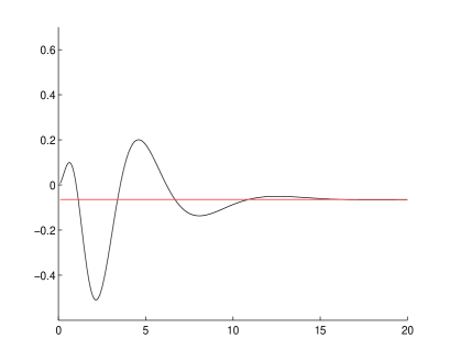
Figure 1. The graph of $H_{\mathbb{S}^{2}}(a)$ is on the left; the remainder term $\left(H_{\mathbb{S}^{2}}(a)-1-\frac{8}{3\pi a}\right)\cdot a^{3}$ is shown on the right, the horizontal red line is $-64/(315\pi)=-0.064$.

Estimate for the torus.

Lemma 4.2.

The following asymptotic expansion holds as $a\to\infty$:

$$\sum_{k\in\mathbb{Z}^{2}_{0}}\frac{1}{\left(\left(\frac{|k|}{\sqrt{a}}\right)^{4}+1\right)^{2}}=\frac{\pi^{2}}{4}a-1+O(e^{-C\sqrt{a}}).$$ (4.3)

Proof.

We use the Poisson summation formula (see, e. g., [15]):

$$\sum_{m\in\mathbb{Z}^{d}}f(m/\nu)=(2\pi)^{d/2}\nu^{d}\sum_{m\in\mathbb{Z}^{d}}\widehat{f}(2\pi m\nu),$$

where $\widehat{f}(\xi)=(2\pi)^{-d/2}\int_{\mathbb{R}^{d}}f(x)e^{-i\xi x}dx$.

Taking into account that the term with $k=(0,0)$ is missing in (4.3), the Poisson summation formula gives

$$\sum_{k\in\mathbb{Z}^{2}_{0}}\frac{1}{\left(\left(\frac{|k|}{\sqrt{a}}\right)^{4}+1\right)^{2}}+1=$$ (4.4)

$$=a\int_{\mathbb{R}^{2}}\frac{dxdy}{((x^{2}+y^{2})^{2}+1)^{2}}+2\pi a\sum_{k\in\mathbb{Z}^{2}_{0}}\widehat{h}(2\pi\sqrt{a}|k|)=\frac{\pi^{2}}{4}a+O(e^{-C\sqrt{a}}),$$

where $h(x,y)=\frac{1}{((x^{2}+y^{2})^{2}+1)^{2}}$ is analytic and therefore its Fourier transform

$$\widehat{h}(\xi)=\frac{1}{2\pi}\int_{\mathbb{R}^{2}}e^{-ix\xi_{1}-iy\xi_{2}}h(x,y)dxdy$$ (4.5)

is exponentially decaying. ∎

The graph of the function

$$H_{\mathbb{T}^{2}}(a):=\frac{4}{\pi^{2}}\,a^{3}\sum_{k\in\mathbb{Z}^{2}_{0}}\frac{1}{\bigl{(}|k|^{4}+a^{2}\bigr{)}^{2}}\,<\,1,$$ (4.6)

and the exponentially small remainder term

$$R(a)=2\pi a\sum_{k\in\mathbb{Z}^{2}_{0}}\widehat{h}(2\pi\sqrt{a}|k|)$$

are shown in Fig. 2

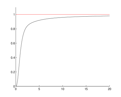
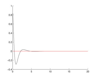
Figure 2. The function $H_{\mathbb{T}^{2}}(a)$ is shown on the left; the exponentially small term $R(a)$ is shown on the right.

We now give an explicit estimate for the exponentially small remainder term in (4.4). The function $h(z)$ is analytic in the domain $\Omega\subset\mathbb{C}^{2}$: $\Omega=\{z\in\mathbb{C}^{2},\ |\mathrm{Im}z_{1}|<\frac{1}{2},\ |\mathrm{Im}z_{2}|<\frac{1}{2}\}$. In fact, the equation

$$(x+i\alpha)^{2}+(y+i\alpha)^{2}=\pm i$$

has real solutions $x$ and $y$ only for $\alpha\geq\frac{1}{2}$.

For $F(x,y,\alpha)=((x+i\alpha)^{2}+(y+i\alpha)^{2})^{2}+1$ we have

$$\mathrm{Re}\,F=(x^{2}+y^{2})^{2}-8\alpha^{2}(x^{2}+y^{2}+xy)+4\alpha^{4}+1\geq t^{2}-12\alpha^{2}t+4\alpha^{4}+1,$$

$$\mathrm{Im}\,F=4a(x+y)(x^{2}+y^{2}-2\alpha^{2}),\quad|\mathrm{Im}\,F|\leq 4\sqrt{2}\alpha t^{1/2}|t-2\alpha^{2}|,$$

where $t:=x^{2}+y^{2}$. Next, by a direct inspection we verify that for $t\geq 0$

$$|F^{2}|\geq(\mathrm{Re}\,F)^{2}-(\mathrm{Im}\,F)^{2}=$$

$$(t^{2}-12\alpha^{2}t+4\alpha^{4}+1)^{2}-32\alpha^{2}t(t-2a^{2})^{2}>\frac{1}{b}(t^{4}+1),$$

where $\alpha=4.6^{-1}$ and $b=4.75$. This gives that for $|\mathrm{Im}z_{1}|\leq\alpha,\ |\mathrm{Im}z_{2}|\leq\alpha$

$$|h(x+i\alpha,y+i\alpha)|\leq\frac{b}{(x^{2}+y^{2})^{4}+1}\,.$$

By the Cauchy integral theorem we can shift the $x$ and $y$ integration in (4.5) in the complex plane by $\pm i\alpha$ (depending on the sign of $\xi_{1}$ and $\xi_{2}$) and find that

$$|\widehat{h}(\xi)|\!\leq\!\frac{b}{2\pi}e^{-(|\xi_{1}|+|\xi_{2}|)\alpha}\!\int_{\mathbb{R}^{2}}\frac{dxdy}{(x^{2}+y^{2})^{4}+1}\!=e^{-(|\xi_{1}|+|\xi_{2}|)\alpha}\frac{b\pi\sqrt{2}}{8}\leq e^{-\alpha|\xi|}\frac{b\pi\sqrt{2}}{8}\,.$$

We write the numbers $|k|^{2}$ over the lattice $\mathbb{Z}^{2}_{0}$ in non-decreasing order and denote them by $\{\lambda_{j}\}^{\infty}_{j=1}$. Using that $\lambda_{j}\geq j/4$ (see [8]) and setting $L:=\frac{\alpha\pi\sqrt{a}}{2}$ and $A:=\frac{\pi^{2}\sqrt{2}ab}{4}$ we estimate the series in (4.4) as follows

$$|R(a)|\leq 2\pi a\sum_{k\in\mathbb{Z}^{2}_{0}}|\widehat{h}(2\pi\sqrt{a}|k|)|=2\pi a\sum_{j=1}^{\infty}|\widehat{h}(2\pi\sqrt{a}\lambda_{j}^{1/2})|\leq$$

$$A\sum_{j=1}^{\infty}e^{-2\pi\alpha\sqrt{a}\lambda_{j}^{1/2}}\leq A\sum_{j=1}^{\infty}e^{-2Lj^{1/2}}=Ae^{-L}\sum_{j=1}^{\infty}e^{-L(2j^{1/2}-1)}\leq$$

$$Ae^{-L}\sum_{j=1}^{\infty}e^{-Lj^{1/2}}<Ae^{-L}\int_{0}^{\infty}e^{-L\sqrt{x}}dx=Ae^{-L}\frac{2}{L^{2}}=\frac{2^{3/2}b}{\alpha^{2}}e^{-\frac{\alpha\pi\sqrt{a}}{2}}\,.$$

Inequality (4.6) holds if $R(a)<1$. The above estimates show that $|R(a)|<1$ for

$$a>\left[\frac{2}{\alpha\pi}\log\left(\frac{2^{3/2}b}{\alpha^{2}}\right)\right]^{2}=273.8\,.$$

A more optimistic estimate follows from the fact that $h(x)$ is radial and therefore so is its Fourier transform

$$\widehat{h}(\xi)=\int_{0}^{\infty}J_{0}(|\xi|r)h(r)rdr,$$

where $J_{0}$ is the Bessel function. The latter integral is expressed in terms of the Meijer G-function and satisfies $|\widehat{h}(\xi)|<e^{-|\xi|/2}$. Similar estimates give that $|R(a)|<1$ for

$$a>\left[\frac{4}{\pi}\log\frac{64}{\pi}\right]^{2}=14.73\,.$$

Acknowledgements

The work of A. I. and S. Z. is supported in part by the Russian Science Foundation grant 19-71-30004 (sections 1,2). Research of A. L. is supported by the Russian Science Foundation grant 19-71-30002 (sections 3,4).

References

- [1] A. Babin and M. Vishik, Attractors of evolution equations. Studies in Mathematics and its Applications, 25. North-Holland Publishing Co., Amsterdam, 1992.
- [2] J. Dolbeault, A. Laptev, and M. Loss, Lieb–Thirring inequalities with improved constants. J. European Math. Soc. 10:4 (2008), 1121–1126.
- [3] R.L. Frank, D. Hundertmark, M. Jex, P.T. Nam. The Lieb–Thirring inequality revisited. arXiv:1808.09017
- [4] R.L. Frank, A. Laptev, and T. Weidl, Lieb–Thirring inequalities, book in preparation.
- [5] A.A.Ilyin, Partly dissipative semigroups generated by the Navier–Stokes system on two-dimensional manifolds and their attractors. Mat. Sbornik 184, no. 1, 55–88 (1993) English transl. in Russ. Acad. Sci. Sb. Math. 78, no. 1, 47–76 (1993).
- [6] A.A. Ilyin, Lieb–Thirring inequalities on some manifolds. J. Spectr. Theory 2 (2012), 57–78.
- [7] A.A. Ilyin and A.A. Laptev, Lieb-Thirring inequalities on the torus. Mat. Sb. 207:10 (2016), 56–79; English transl. in Sb. Math. 207:9-10 (2016).
- [8] A.A. Ilyin and A.A. Laptev, Lieb–Thirring inequalities on the sphere. Algebra i Analiz 31:3 (2019), 116–135; English transl. in St. Petersburg Mathematical Journal 31:3 (2020.)
- [9] A. Laptev and T. Weidl, Sharp Lieb–Thirring inequalities in high dimensions. Acta Math. 184 (2000), 87–111.
- [10] E.H. Lieb, On characteristic exponents in turbulence. Comm. Math. Phys. 92 (1984), 473–480.
- [11] E. Lieb, M. Loss, Analysis. Second edition. Graduate Studies in Mathematics, 14. American Mathematical Society, Providence, RI, 2001.
- [12] E. Lieb and W. Thirring, Inequalities for the moments of the eigenvalues of the Schrödinger Hamiltonian and their relation to Sobolev inequalities, Studies in Mathematical Physics. Essays in honor of Valentine Bargmann, Princeton University Press, Princeton NJ, 269–303 (1976).
- [13] Sh.M. Nasibov, On optimal constants in some Sobolev inequalities and their application to a nonlinear Schrödinger equation, Dokl. Akad. Nauk SSSR. 307 (1989), 538–542; English transl. in Soviet Math. Dokl. 40 (1990).
- [14] M. Rumin, Balanced distribution-energy inequalities and related entropy bounds. Duke Math. J. 160 (2011), 567–597.
- [15] E.M. Stein and G. Weiss, Introduction to Fourier analysis on Euclidean spaces. Princeton University Press, Princeton NJ, 1972.
- [16] R. Temam, Infinite Dimensional Dynamical Systems in Mechanics and Physics, 2nd ed., Springer-Verlag, New York, 1997.
- [17] M. Weinstein, Nonlinear Schrödinger equations and sharp interpolation estimates Comm. Math. Phys. 87 (1983), 567–576.
- [18] S.V. Zelik, A.A.Ilyin. Green’s function asymptotics and sharp interpolation inequalities. Uspekhi Mat. Nauk 69:2 (2014), 23–76; English transl. in Russian Math. Surveys 69:2 (2014).
- [19] S.V. Zelik, A.A. Ilyin, and A.A. Laptev. On the Lieb–Thirring constant on the torus. Mat. zametki. 106:6 (2019), 946–950; English transl. in Math. notes 106:6 (2019).