A hybrid WENO method with modified ghost fluid method for compressible two-medium flow problems

Zhuang Zhao, Yibing Chen and Jianxian Qiu

Abstract

In this paper, we develop a simplified hybrid weighted essentially non-oscillatory (WENO) method combined with the modified ghost fluid method (MGFM) [28] to simulate the compressible two-medium flow problems. The MGFM can turn the two-medium flow problems into two single-medium cases by defining the ghost fluids status in terms of the predicted the interface status, which makes the material interface “invisible”. For the single medium flow case, we adapt between the linear upwind scheme and the WENO scheme automatically by identifying the regions of the extreme points for the reconstruction polynomial as same as the hybrid WENO scheme [50]. Instead of calculating their exact locations, we only need to know the regions of the extreme points based on the zero point existence theorem, which is simpler for implementation and saves computation time. Meanwhile, it still keeps the robustness and has high efficiency. Extensive numerical results for both one and two dimensional two-medium flow problems are performed to demonstrate the good performances of the proposed method.

Key Words: hybrid WENO scheme, two-medium flow problems, modified ghost fluid method, zero point existence theorem

AMS(MOS) subject classification: 65M60, 35L65

1 Introduction

In this paper, we propose a simplified hybrid weighted essentially non-oscillatory (WENO) method with modified ghost fluid method (MGFM) [28] for simulating compressible two-medium flow problems. For two-medium flow problems, the equation of state (EOS) would switch between the different medium, which may cause numerical oscillations or inaccuracies near the material interface. Hence, many researchers have used various additional works and techniques to overcome this difficulty, and there are two major options to simulate the compressible two-medium flow problems.

One is the front capturing method, where the high resolution methods are applied to suppress the non-physical oscillations near discontinuities by bringing the numerical diffusion or viscosity, which inherently exists in the method itself or is given artificially. The front capturing method can deal with large deformation problems and relatively easy to extend to high dimension. However, the numerical inaccuracies and oscillations are inevitable near the interface, therefore, various techniques were introduced by Larrouturou [20], Karni [19], Abgrall et al. [1, 2], Shyue et al. [40], Saurel et al. [36] and Chen et al. [5] to resolve this difficulty. The other one is the front tracking method, which terms the discontinuities between the two-medium flows as internal moving interfaces. It works well at multi-material interfaces, but it would have difficulties about the entanglement of the Lagrangian meshes and the extension to high dimension, and there are some typical methods about the front tracking method, such as volume of fluid (VOF) method [13], level set method [41] and other front tracking methods [42, 7].

To combine the best properties of the front capturing and tracking methods, Fedikw et al. [6] proposed a new numerical method for treating interfaces using a level set function in Eulerian schemes named as the ghost fluid method (GFM), which makes the interface “invisible”. In the framework of the GFM [6], the pressure and velocity at the ghost fluid nodes near the interface are defined as the local real pressure and velocity, while the density is obtained by isobaric fixing. It can easily turn the two-medium flow problems into two single-medium flow cases, and for the single-medium flow problems, many classical and mature schemes can be applied. Hence, it provides an alternative and flexible way to simulate the two-medium flow problems, and the extension to high dimension becomes fairly straightforward. However, it may cause numerical inaccuracies in the case of a strong shock impacting on the interface, and the reason may be that the statuses near the interface are affected by the wave interaction and the material properties on both sides. Therefore, Liu et al. [28] developed a modified ghost fluid method (MGFM), in which a multi-material Riemann problem is defined and solved approximately or exactly to predict the interfacial status, then, the predicted interfacial status is applied to define the fluid values at the ghost points. The MGFM combines the advantages of the GFM [6] and the implicit characteristic methods [26, 27], and it takes the interaction of shock with the interface into consideration. Later, the interface interaction GFM (IGFM) [14], the real GFM (RGFM) [43] and the practical GFM (PGFM) [44] were developed following the idea of the Riemann problem-based technique in the MGFM [28]. The MGFM is robust and less problem related, and it has been applied in various situations as in [25, 30, 33, 46, 23], and the accuracy analysis and errors estimation can be seen in [24, 45]. The GFM [6] and its relevant ghost fluid methods [28, 14, 43, 44] are non-conservative near the interface, and the conservative scheme can be seen in [32].

Here, we would use the MGFM to define the ghost fluid status for the two-medium flow problems considering its great performances, and for the single-medium flow problems, many successful numerical schemes can be applied for it. Among them, the finite difference or finite volume weighted essentially non-oscillatory (WENO) schemes have been widely applied for the single-medium flow problems which usually contain shock, contact discontinuities and sophisticated smooth structures simultaneously. And in 1994, the first WENO scheme was constructed by Liu, Osher and Chan [29] on the basis of ENO schemes [11, 9, 10], where all candidate stencils were used with a nonlinear convex methodology to obtain higher order accuracy in the smooth regions, then, Jiang and Shu [17] proposed the third and fifth-order finite difference WENO schemes in multi-space dimension, in which a general definition for smoothness indicators and nonlinear weights was presented. After this, WENO schemes have been further developed in [15, 21, 37, 47, 3, 49, 51]. However, the cost of computing the nonlinear weights and local characteristic decompositions is still very high. Hence, Hill and Pullin [12] combined the tuned center-difference schemes with WENO schemes to expect that the nonlinear weights would be achieved automatically in the smooth regions away from shocks, but a switching principle was still significant. Later, Li and Qiu [22] studied the hybrid WENO scheme using different switching principles [34], which shows different principles would have different influences for the hybrid WENO scheme [22], and the majorities of the troubled-cell indicators need to adjust parameters for different problems to balance better non-oscillations near discontinuities and less computation cost, simultaneously. Hence, Qiu et al. [50, 48] used a new simple switching principle, which employed different reconstruction method automatically based on the locations of all extreme points of the big reconstruction polynomial for numerical flux. Then, we develop this methodology in this paper, in which we only need to know the regions of the extreme points, rather than calculating their exact locations as in [50, 48].

In this paper, to keep the robustness of the MGFM [28] and high efficiency of the hybrid WENO schemes [50, 48], we first use the methodology introduced in [28] to predict the interfacial status based on a multi-material Riemann problem, then, the predicted interfacial status is applied to define the ghost fluid values, by which it turns a two-medium flow problems into two single-medium cases. For the single-medium problems, we would solve it by the hybrid WENO method, where we reconstruct the numerical flux by upwind linear approximation directly if all extreme points of the big reconstruction polynomial for numerical flux are located outside of the big stencil, otherwise we use the classical WENO procedure [17]. But we only need to know the regions of the extreme points in terms of the zero point existence theorem, instead of calculating their exact locations as in [50, 48], and it is more easy for implementation and saves computation time. Meanwhile, it still keeps the robustness of the WENO scheme [17] and the MGFM [28] to simulate the two-medium flow problems. In addition, it has higher efficiency with less computation costs than the WENO scheme [17] for employing linear approximation straightforwardly in the smooth regions.

The organization of the paper is as follows: in Section 2, the detailed implementation procedures of the finite difference hybrid WENO scheme combined with the MGFM are presented for two-medium flow problems. In Section 3, Extensive numerical results for gas-gas and gas-water interaction problems in one and two dimensions are presented to illustrate good performances of the proposed scheme. Concluding remarks are given in Section 4.

2 Numerical Methods

We first introduce the governing equations for the compressible two-medium flow problems, then, we give a brief review about the finite difference hybrid WENO method [50] for single-medium flow problems, but we have an improvement about the identification technique for the regions of the extreme points of the big reconstruction polynomial. Next, we introduce the level set technique to track the moving interface, then, we briefly introduce the modified ghost fluid method (MGFM) [28] to define the status of ghost fluids. Finally, we give the summary of the implementation procedures.

2.1 Governing equations

We consider the hyperbolic conservations laws given as follows

$$\left\{\begin{array}[]{ll}U_{t}+\nabla\cdot F(U)=0,\\ U(x,0)=U_{0}(x),\\ \end{array}\right.$$ (2.1)

where $U$ is $(\rho,\rho\mu,E)^{T}$ and $F(U)$ is $(\rho\mu,\rho\mu^{2}+p,\mu(E+p))^{T}$ for one dimensional Euler equations, while for two dimensional Euler equations, $U$ is $(\rho,\rho\mu,\rho\nu,E)^{T}$, and $F(U)$ is $(F_{1}(U),F_{2}(U))$ with $F_{1}(U)=(\rho\mu,\rho\mu^{2}+p,\rho\mu\nu,\mu(E+p))^{T}$, $F_{2}(U)=(\rho\nu,\rho\mu\nu,\rho\nu^{2}+p,\nu(E+p))^{T}$. In order to close the systems, the equations of state (EOS) is still required. The $\gamma$-law for gas is

$$\rho e=p/(\gamma-1),$$

and Tait EOS for the water medium [4, 6, 26] is given as

$$\rho e=(p+N\bar{B})/(N-1),$$

in which $\bar{B}=B-A$, $N=7.15$, $A=1.0\times 10^{5}$ Pa, $A=3.31\times 10^{8}$ Pa, and $\rho_{0}=1000.0kg/m^{3}$.

2.2 Hybrid WENO scheme for single-medium flow

We first consider one dimensional scalar hyperbolic conservation laws

$$\left\{\begin{array}[]{ll}u_{t}+f_{x}(u)=0,\\ u(x,0)=u_{0}(x).\\ \end{array}\right.$$ (2.1)

We divide the computing domain by uniform grid points $\{x_{i}\}$, and $h$ is denoted as $x_{i+1}-x_{i}$. The cell $I_{i}$ is defined as $[x_{i-1/2},x_{i+1/2}]$, where $x_{i+1/2}$ is set as $x_{i+1/2}=x_{i}+h/2$, then, the semi-discrete finite difference scheme of (2.1) is written as

$$\frac{du_{i}(t)}{dt}=-\frac{1}{h}\left(\hat{f}_{i+1/2}-\hat{f}_{i-1/2}\right),$$ (2.2)

in which $u_{i}(t)$ is represented as $u(x_{i},t)$, and the numerical flux $\hat{f}_{i+1/2}$ is a fifth order approximation of $v_{i+1/2}=v(x_{i+1/2})$, in which $v(x)$ is defined implicitly as in [17]:

$$f(u(x))=\frac{1}{h}\int_{x-h/2}^{x+h/2}v(x)dx,$$

then, the right hand item of (2.2) is the fifth order approximation for $-f_{x}(u)$ at $x_{i}$. For the stability of the finite difference scheme, we split the flux $f(u)$ into two parts: $f(u)=f^{+}(u)+f^{-}(u)$, in which $\frac{df^{+}(u)}{du}\geq 0$ and $\frac{df^{-}(u)}{du}\leq 0$, and the Lax-Friedrichs flux splitting method is applied here as

$$f^{\pm}(u)=\frac{1}{2}(f(u)\pm\alpha u),$$

where $\alpha=$ $\max_{u}|f^{\prime}(u)|$.

Next, we introduce the detailed procedures for the reconstruction of the numerical flux $\hat{f}^{+}_{i+1/2}$, which is the fifth order approximation of $f^{+}(u(x_{i+1/2}))$, and the reconstruction formulas for $\hat{f}^{-}_{i+1/2}$ are mirror symmetric with respect to $x_{i+1/2}$ of that for $\hat{f}^{+}_{i+1/2}$. $\hat{f}_{i+1/2}$ is finally taken as $\hat{f}^{+}_{i+1/2}+\hat{f}^{-}_{i+1/2}$. Now, we first give a big stencil: $S_{0}=\{I_{i-2},...,I_{i+2}\}$, then we can easily obtain the fourth degree polynomial $p_{0}(x)$ in terms of the following requirements as

$$\frac{1}{h}\int_{I_{j}}p_{0}(x)dx=f^{+}(u_{j}),\ j=i-2,...,i+2.$$

For simplicity, $\frac{(x-x_{i})}{h}$ is set as $\xi$, then we have

$$\begin{split}p_{0}(x)=&\frac{1}{1920}[(-116f^{+}_{i-1}+9f^{+}_{i-2}+2134f^{+}_{i}-116f^{+}_{i+1}+9f^{+}_{i+2})-\\ &40(34f^{+}_{i-1}-5f^{+}_{i-2}-34f^{+}_{i+1}+5f^{+}_{i+2})\xi+120(12f^{+}_{i-1}-\\ &f^{+}_{i-2}-22f^{+}_{i}+12f^{+}_{i+1}-f^{+}_{i+2})\xi^{2}+160(2f^{+}_{i-1}-f^{+}_{i-2}-\\ &2f^{+}_{i+1}+f^{+}_{i+2})\xi^{3}-80(4f^{+}_{i-1}-f^{+}_{i-2}-6f^{+}_{i}+4f^{+}_{i+1}-f^{+}_{i+2})\xi^{4})].\end{split}$$

To increase the efficiency, we also use the thought of the hybrid WENO schemes [50, 48], in which the linear upwind approximation or WENO reconstruction is applied automatically based on the locations of the extreme points of the big polynomial $p_{0}(x)$. More explicitly, if all extreme points are located outside of the big spatial stencil $S_{0}$, $\hat{f}^{+}_{i+1/2}$ is taken as $p_{0}(x_{i+\frac{1}{2}})$ directly, otherwise the classical WENO procedures [17] would be used to reconstruct it. Unlike the hybrid WENO schemes [50, 48] solving the real zero points of $p_{0}^{\prime}(x)$ exactly, we identify the regions of the extreme points of $p_{0}(x)$ in terms of the zero point existence theorem as that if the endpoint values of $p^{\prime}_{0}(x)$ and the extreme values of $p^{\prime}_{0}(x)$ have same signs on the big stencil $S_{0}$, it means there is no single zero points of $p_{0}^{\prime}(x)$ on $S_{0}$, that is to say, there is no extreme points of $p_{0}(x)$ located in $S_{0}$. Also, we present their performances in the numerical examples, which shows the new identification skill can catch the regions for the extreme points of the big polynomial $p_{0}(x)$ as the old one in [50, 48], but it has higher efficiency. In addition, the new one has simpler implementation procedure as it only needs to solve the zero points of the quadratic polynomial $p_{0}^{\prime\prime}(x)$, while the old one has to calculate the roots of the cubic polynomial $p_{0}^{\prime}(x)$.

Then, we review the classical WENO procedure [17] for the reconstruction of $\hat{f}^{+}_{i+1/2}$. Firstly, the big stencil $S_{0}$ is divided into three smaller stencils: $S_{1}=\{I_{i-2},I_{i-1},I_{i}\}$, $S_{2}=\{I_{i-1},I_{i},I_{i+1}\}$ and $S_{3}=\{I_{i},I_{i+1},I_{i+2}\}$, then, the polynomials $p_{l}(x)$ are obtained by the following requirements as

$$\frac{1}{h}\int_{I_{j}}p_{l}(x)dx=f^{+}(u_{j}),\ j=i-3+l,...,i-1+l,\ l=1,2,3.$$

The explicit values of $p_{l}(x)$ at the point $x_{i+1/2}$ can be seen in [17], and the linear weights are computed by $p_{0}(x_{i+1/2})=\sum_{l=1}^{3}\gamma_{l}p_{l}(x_{i+1/2})$, in which $\gamma_{1}=\frac{1}{10}$, $\gamma_{1}=\frac{3}{5}$ and $\gamma_{2}=\frac{3}{10}$. To measure how smooth these small polynomials $p_{l}(x)$ are in the target cell $I_{i}$, we use the same definition of smoothness indicators $\beta_{l}$ seen in [17, 38] as

$$\beta_{l}=\sum_{\alpha=1}^{2}\int_{I_{i}}h^{2\alpha-1}(\frac{d^{\alpha}p_{l}(x)}{dx^{\alpha}})^{2}dx,$$

then, the nonlinear weights are

$$\omega_{l}=\frac{\overline{\omega}_{l}}{\sum_{k=0}^{r}\overline{\omega}_{k}},\,\,\,\overline{\omega}_{l}=\frac{\gamma_{l}}{(\beta_{l}+\varepsilon)^{2}},\ l=1,2,3,$$

where $\varepsilon=10^{-6}$, and the explicit values of $\omega_{l}$ also can be seen in [17]. Finally, the WENO reconstruction of $\hat{f}^{+}_{i{+}1/2}$ is

$$\hat{f}^{+}_{i{+}1/2}=\sum_{l=1}^{3}\omega_{l}p_{l}(x_{i+1/2}).$$

After the spatial discretization, the semi-discrete scheme (2.2) is discretized by the third order TVD Runge-Kutta method [39] in time as

$$\left\{\begin{array}[]{lll}u^{(1)}&=&u^{n}+\Delta tL(u^{n}),\\ u^{(2)}&=&\frac{3}{4}u^{n}+\frac{1}{4}u^{(1)}+\frac{1}{4}\Delta tL(u^{(1)}),\\ u^{(n+1)}&=&\frac{1}{3}u^{n}+\frac{2}{3}u^{(2)}+\frac{2}{3}\Delta tL(u^{(2)}).\end{array}\right.$$ (2.6)

Remark 1: For the systems, such as the one dimensional compressible Euler equations, WENO procedure is performed in the local characteristic directions to overcome the oscillations nearby discontinuities as in [17], while the linear approximation is directly computed in each component. For two dimensional problems, the spatial reconstruction is performed by dimension by dimension.

2.3 Level set equation

We choose the next level set technique to track the moving interface. For one dimensional problems, the level set equation is

$$\phi_{t}+u\phi_{x}=0,$$ (2.7)

while for two dimensional case it is written as

$$\phi_{t}+u\phi_{x}+v\phi_{x}=0,$$ (2.8)

where $\phi$ is a signed distance function. $u$ and $v$ are the velocity of the flow in the $x$ and $y$ directions, respectively. We would solve the equations (2.7) and (2.8) by the fifth order finite difference hybrid WENO method introduced in Appendix A. However, if the velocity field has a large gradient in the vicinity of the interface, the level set method may cause seriously distorted contours. Therefore, the re-initialization technique is needed to remedy this influence. For one dimensional problems, we can obtain the position of the interface exactly by Newton’s iteration method, then we re-distribute the signed distance function $\phi$. For two dimensional case, the interface is a curve, so we need to use other ways for re-initialization, in which we solve the re-initialization equation as:

$$\phi_{t}+S(\phi_{0})(\sqrt{\phi_{x}^{2}+\phi_{y}^{2}}-1)=0,$$ (2.9)

where $S$ is the sign function of $\phi_{0}$, and the equation (2.9) is also calculated by the hybrid WENO method shown in Appendix A.

2.4 Modified Ghost Fluid Method

We use the modified ghost fluid method (MGFM) [28] to define the information of the ghost cells as it considers the interaction of shock with the interface correctly. The main procedures of the MGFM are that we first predict the interface status by solving a two-medium Riemann problem exactly or approximately, then, the predicted interface status is used to define the ghost fluid status for each fluid, by which it turns a two-medium flow problem into two single-medium flow problems.

Figure 2.1: Isentropic fixing for 1D two-medium flow problems.

For one dimensional case, we only introduce how to define the ghost fluid status for Medium 1 in detail, and the definition of the ghost fluid status for Medium 2 is similar. Let’s assume that the interface is located between $i$ and $i+1$ seen in Figure 2.1, then, we use the status of $U_{i-1}$ and $U_{i+2}$ to define the two-medium Riemann problem suggested in [28], and obtain the interfacial status: $u_{i}$ (velocity), $p_{i}$ (pressure), $\rho_{i}^{L}$ (density at left-side) and $\rho_{i}^{R}$ (density at right-side). Later, we take the predicted $u_{i}$, $p_{i}$, $\rho_{i}^{L}$ as the velocity, pressure and density at the ghost point $i+1$, but at these points $i$, $i+2$ and $i+3$, the pressure and velocity are those on the real local fluid, and the density at these points is replaced by the isentropic fixing [6, 28].

For two dimensional case, it would have one difficulty about the definition of the two-medium Riemann problem for there is two velocity components. However, we can know the normal direction $\overrightarrow{n}$ near the interface employing the level set function ($\overrightarrow{n}=\nabla\phi/|\nabla\phi|$), then, we obtain the normal velocity $u_{N}$ and tangential velocity $u_{T}$, in which $u_{N}$ is defined as $(\mu,\nu)\cdot\overrightarrow{n}$, then, we apply the normal velocity $u_{N}$, the pressure $p$ and the density $\rho$ to define the two-medium Riemann problem like one dimensional case. In terms of the MGFM [28], we need to define a computation domain for each medium that includes boundary points and grid points in the interfacial regions by $|\phi|<\epsilon$, where $\epsilon$ is set to be 3$\max(\Delta x,\Delta y)$ for the fifth order hybrid WENO scheme. Later, we would only introduce the definition of the status for Medium 1 at the points $A$ and $B$ (seen in Figure 2.2) in detail. To define the status at the point $A$ in Medium 1, we need to find other point next to the interface ($|\phi|<\epsilon$) located in the Medium 2, and let’s assume that $B$ is the target point as the angle made by the normal of $B$ and $A$ is the minimum, then we define Riemann problem in the normal direction as

$$U|_{t=t_{n}}=\left\{\begin{array}[]{ll}U_{A},\\ U_{B},\\ \end{array}\right.$$

in which $U_{A}$ = $(\rho^{A},u_{N}^{A},p^{A})$ and $U_{B}$ = $(\rho^{B},u_{N}^{B},p^{B})$, then we can solve it approximately or exactly to predict the status $u_{I}$ (velocity), $p_{I}$ (pressure), $\rho_{I}^{L}$ (density at left-side) and $\rho_{I}^{R}$ (density at right-side). Notice that node $A$ is located in Medium 1, then, we only need to define the density by isentropic fixing [6, 28], but node $B$ is located in Medium 2, therefore, we need to define the status at node $B$ by $u_{I}$, $p_{I}$ and $\rho_{I}^{L}$, and its tangential velocity is still the original one. In addition, the definition of the ghost fluid status for Medium 2 is similar.

Figure 2.2: Isentropic fixing for 2D two-medium flow problems.

2.5 Summary of the Procedures

Now, we give a brief summary of the procedures for simulating two-medium flow problems. Let’s assume that the flow status at $t_{n}$ has been obtained, then we can advance the respective quantities to $t_{n+1}$ following as:

Step 1. Calculate the time step $\Delta t$, satisfying the stability condition over the whole range.

Step 2. Solve the level set function $\phi$, and obtain the locations of the interface in the next intermediate time step introduced in Section 2.3.

Step 3. Define the Riemann problem near the interface and predict the interface status, then use it to define the fluid values at the ghost points for Mediums 1 and 2, respectively, given in Section 2.4.

Step 4. Solve the governing equations for Mediums 1 and 2, respectively, advancing the solution to the next intermediate time level, shown in Section 2.2.

Step 5. Repeat Steps 2, 3 and 4 at each intermediate time step of the third order TVD Runge-Kutta method, and advance the solution from $U_{n}$ to $U_{n+1}$, then, re-initialize the level set function $\phi$.

3 Numerical Results

In this section, we perform the numerical results of the new simplified hybrid WENO scheme and classical WENO scheme [17] with the modified ghost fluid method for two-medium flow problems which are outlined in the previous section, and the CFL number is set as 0.6. In addition, we also make a comparison between the new identification skill for the regions of the extreme points introduced in the previous section and the old one used in the hybrid WENO schemes [50, 48]. The units for the density, velocity, pressure, length and time are kg$/\text{m}^{3}$, m/s, Pa, m, and s, respectively.

Here, we use “New/simplified hybrid WENO method” to denote the new simplified finite difference hybrid WENO scheme with the modified ghost fluid method developed in this paper, and use “Classical WENO method” to represent the classical finite difference WENO scheme [17] with the modified ghost fluid method. In addition, we use “Old hybrid WENO method” to denote the finite difference hybrid WENO scheme [50] with the modified ghost fluid method.

Example 3.1. This problem was taken from [6], and the initial conditions are

$$(\rho,\mu,p,\gamma)=\left\{\begin{array}[]{ll}(1,0,1\times 10^{5},1.4),&x\in[0,0.5),\\ (0.125,0,1\times 10^{4},1.2),&x\in[0.5,1].\end{array}\right.$$

In flow and out flow boundary conditions are applied here, and the final computed time $t$ is 0.0007. We present the computed density $\rho$, velocity $\mu$ and pressure $p$ by New/Simplified hybrid WENO and Classical WENO methods against the exact solution in Figure 3.1. We can find that the two methods both capture the location of the material interface correctly. These two schemes also have similar numerical results, and the overall results are comparable to analysis, but New/simplified hybrid WENO method can achieve higher efficiency than Classical WENO method for saving 22.93% computation time. In addition, we find New/simplified hybrid WENO method can save 9.25% CPU time than Old hybrid WENO method by calculation, meanwhile, there are only 15.13% and 15.14% points where the WENO procedures are computed in New/simplified hybrid WENO and Old hybrid WENO methods, respectively, and the time history of the locations of WENO reconstruction for two methods are given in the top of Figure 3.4. These results show that the new identification skill in New/simplified hybrid WENO method can identify the regions of the extreme points correctly as the old one in Old hybrid WENO method, but the new one has higher efficiency. The new identification technique is also simpler as it only needs to solve the zero points of a quadratic polynomial, while the old one has to calculate the roots of a cubic polynomial.

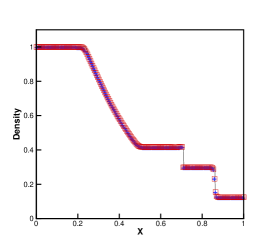
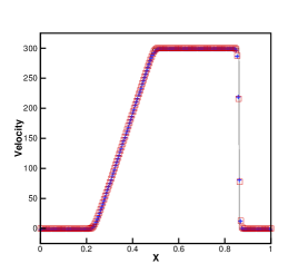
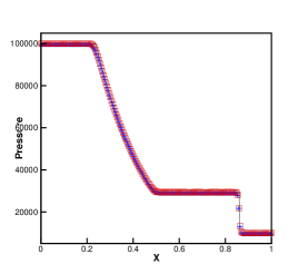
Figure 3.1: Example 3.1. t=0.0007. From left to right: density; velocity; pressure. Solid line: the exact solution; plus signs: the results of Classical WENO method; squares: the results of New/simplified hybrid WENO method. Grid points: 200.

Example 3.2. This problem is also taken from [6], which contains a right going shock refracting at an air-helium interface with a reflected rarefaction wave, and the initial conditions are given as

$$(\rho,\mu,p,\gamma)=\left\{\begin{array}[]{ll}(4.3333,3.2817\sqrt{10^{5}},1.5\times 10^{6},1.4),&x\in[0,0.05),\\ (1,0,1\times 10^{5},1.4),&x\in[0.05,0.5),\\ (0.1379,0,1\times 10^{5},5/3),&x\in[0.5,1],\\ \end{array}\right.$$

with inflow/outflow boundary conditions. The initial strength of the shock is $p_{l}/p_{R}=15$ at $x=0.05$, and the interface of air and helium is located at $x=0.5$. We ran the code to a final time of 0.0005, and the computed density $\rho$, velocity $\mu$ and pressure $p$ by New/simplified hybrid WENO and Classical WENO methods against the exact solution are shown in Figure 3.2. We can see the contact discontinuity is located in the correct cell, and two methods have similar results, but New/simplified hybrid WENO method can achieve higher efficiency than Classical WENO method for saving 16.41% CPU time. In addition, we find New/simplified hybrid WENO method can save 9.54% computation time than Old hybrid WENO method by calculation, meanwhile, there are 25.07% and 24.50% points where the WENO procedures are computed in New/simplified hybrid WENO and Old hybrid WENO methods, respectively, and the time history of the locations of WENO reconstruction are shown in the middle of Figure 3.4, which illustrate that the new identification skill in New/simplified hybrid WENO method catchs the regions of the extreme points as the old one in Old hybrid WENO method. However, the new identification technique has higher efficiency, and it is also simpler for it only needs to calculate the roots of a quadratic polynomial.

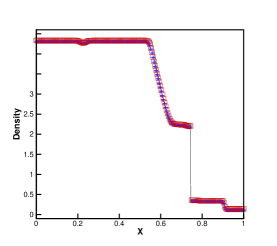
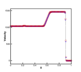
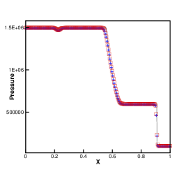
Figure 3.2: Example 3.2. t=0.0005. From left to right: density; velocity; pressure. Solid line: the exact solution; plus signs: the results of Classical WENO method; squares: the results of New/simplified hybrid WENO method. Grid points: 200.

Example 3.3. We solve the governing equations (2.1) for one dimensional Euler equations with the following Riemann initial conditions

$$(\rho,\mu,p,\gamma)=\left\{\begin{array}[]{ll}(1.3333,0.3535\sqrt{10^{5}},1.5\times 10^{5},1.4),&x\in[0,0.05),\\ (1,0,1\times 10^{5},1.4),&x\in[0.05,0.5),\\ (3.1538,0,1\times 10^{5},1.249),&x\in[0.5,1],\\ \end{array}\right.$$

The final computed time $t$ is up to 0.0017. This example is also taken from [6], and the computed density $\rho$, velocity $\mu$ and pressure $p$ by New/simplified hybrid WENO and Classical WENO methods against the exact solution are given in Figure 3.3. The numerical results illustrate two schemes capture the contact discontinuity correctly, with non-oscillations and similar comparable results, meanwhile, New/simplified hybrid WENO method saves almost 25.49% computation time comparing with Classical WENO method. In addition, we find New/simplified hybrid WENO method with the new identification skill can save 8.31% CPU time than Old hybrid WENO method by calculation, meanwhile, there are only 8.48% and 8.52% points where the WENO procedures are computed in New/simplified hybrid WENO and Old hybrid WENO methods, respectively. The time history of the locations of WENO reconstruction by the two hybrid methods are seen in the bottom of Figure 3.4. These results illustrate that the new identification technique in New/simplified hybrid WENO method catches the regions of the extreme points as the old one in Old hybrid WENO method, but New/simplified hybrid WENO method with the new one has higher efficiency, and the new identification technique is also simpler.

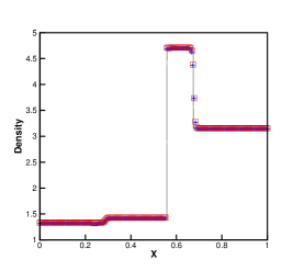
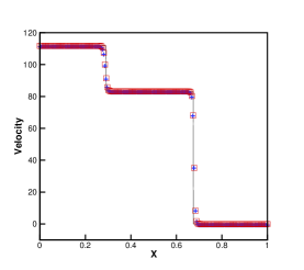
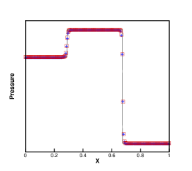
Figure 3.3: Example 3.3. T=0.0017. From left to right: density; velocity; pressure. Solid line: the exact solution; plus signs: the results of Classical WENO method; squares: the results of New/simplified hybrid WENO method. Grid points: 200.

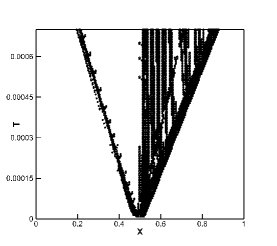
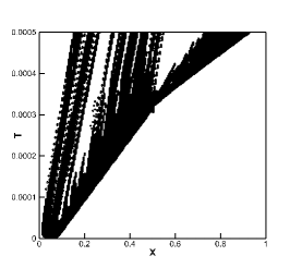
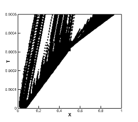
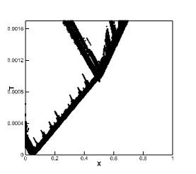
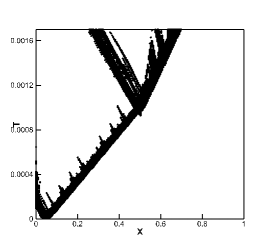
Figure 3.4: The points where the WENO procedures are performed for Examples 3.1 to 3.3. From left to right: the results of Old hybrid WENO method; the results of New/simplified hybrid WENO method.

Example 3.4. This problem is taken from [28], having a strong shock on a gas-gas interface, and the strength of the right shock wave is up to $p_{L}/p_{R}=100$. The initial conditions are given as follows

$$(\rho,\mu,p,\gamma)=\left\{\begin{array}[]{ll}(0.3884,27.1123\sqrt{10^{5}},1.0\times 10^{7},5/3),&x\in[0,0.3),\\ (0.1,0,1\times 10^{5},5/3),&x\in[0.3,0.4),\\ (1,0,1\times 10^{5},1.4),&x\in[0.4,1].\\ \end{array}\right.$$

In Figure 3.5, we present the computed density $\rho$, velocity $\mu$ and pressure $p$ by New/simplified hybrid WENO and Classical WENO methods against the exact solution at the final time $0.0001$. We can find that two methods work well for simulating this two-phase flow problem, and they capture the correct location of the interface between two gases. Comparing with Classical WENO method, New/simplified hybrid WENO method saves almost 15.98% computation time. In addition, we find New/simplified hybrid WENO method with the new identification skill can save 14.52% CPU time than Old hybrid WENO method by calculation, meanwhile, there are 26.76% and 25.52% points where the WENO procedures are performed in New/simplified hybrid WENO and Old hybrid WENO methods, respectively, and the time history of the locations of WENO reconstruction by two hybrid methods are given in the top of Figure 3.8, which illustrate the new identification skill in New/simplified hybrid WENO method identifies the regions of the extreme points as the old one in Old hybrid WENO method, but New/simplified hybrid WENO method with the new one has higher efficiency. The new identification technique in New/simplified hybrid WENO method is also simpler as it only needs to solve the roots of a quadratic polynomial, while the old one in Old hybrid WENO method has to calculate the zero points of a cubic polynomial.

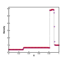
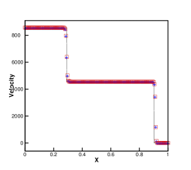
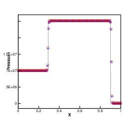
Figure 3.5: Example 3.4. t=0.0001. From left to right: density; velocity; pressure. Solid line: the exact solution; plus signs: the results of Classical WENO method; squares: the results of New/simplified hybrid WENO method. Grid points: 200.

Example 3.5. We consider the gas-water shock tube problem taken from [33], and the initial condition are given as

$$(\rho,\mu,p,\gamma)^{T}=\left\{\begin{array}[]{ll}(1270,0,8\times 10^{8},1.4)^{T},&x\in[0,0.5),\\ (1000,0,1\times 10^{5},7.15)^{T},&x\in[0.5,1].\end{array}\right.$$

This underwater explosion problem has extremely high pressure in the gas medium, therefore, there is a very strong shock in the water. The final computation time is $0.00016$. We present the computed density $\rho$, velocity $\mu$ and pressure $p$ by New/simplified hybrid WENO and Classical WENO methods against the exact solution in Figure 3.6, which illustrates two schemes capture the location of the material interface correctly, and they have good performance in the smooth and discontinuous regions. In addition, New/simplified hybrid WENO method saves about 16.53% CPU time. Moreover, we find New/simplified hybrid WENO method with the new identification skill can save 13.93% computation time than the Old hybrid WENO method with the old identification technique by calculation, meanwhile, there are both 20.68% points where the WENO procedures are performed in New/simplified hybrid WENO and Old hybrid WENO methods, respectively, and the time history of the locations of WENO reconstruction in two hybrid methods are given in the middle of Figure 3.8. These results show that the new identification skill in New/simplified hybrid WENO can catch the regions of the extreme points as the old one in Old hybrid WENO method. However, New/simplified hybrid WENO method with the new identification skill has higher efficiency, and the procedure of the new one is also simpler.

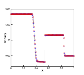
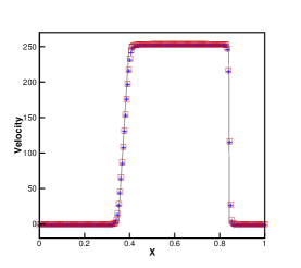
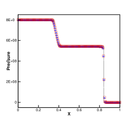
Figure 3.6: Example 3.5. t=00016. From left to right: density; velocity; pressure. Solid line: the exact solution; plus signs: the results of Classical WENO method; squares: the results of New/simplified hybrid WENO method. Grid points: 200.

Example 3.6. This gas-water shock tube problem is taken from [6], which has higher energy of the explosive gaseous medium than the problem given in Example 3.5, and the initial conditions are

$$(\rho,\mu,p,\gamma)^{T}=\left\{\begin{array}[]{ll}(1630,0,7.81\times 10^{9},1.4)^{T},&x\in[0,0.5),\\ (1000,0,1\times 10^{5},7.15)^{T},&x\in[0.5,1].\end{array}\right.$$

We ran the code to the final time 0.0001, then, we give the computed density $\rho$, velocity $\mu$ and pressure $p$ by New/simplified hybrid WENO and Classical WENO methods against the exact solution in Figure 3.7, which shows two schemes work well for this tough gas-water problem with non-oscillation in the non-smooth regions, and they also capture the right interface between two mediums. In addition, New/simplified hybrid WENO method has higher efficiency for saving almost 15.12% CPU time. Moreover, we find New/simplified hybrid WENO method with the new identification skill can save 13.52% computation time than the Old hybrid WENO method by calculation, meanwhile, there are both 32.88% points where the WENO procedures are computed in two hybrid WENO method, and the time history of the locations of WENO reconstruction in New/simplified hybrid WENO and Old hybrid WENO methods are given in the bottom of Figure 3.8, which show that the new identification skill New/simplified hybrid WENO method can catch the regions of the extreme points correctly as the old one, but New/simplified hybrid WENO method with the new one has higher efficiency, and the new identification technique is also simpler.

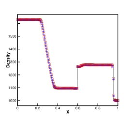
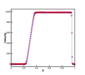
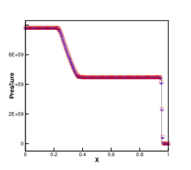
Figure 3.7: Example 3.6. t=0.0001. From left to right: density; velocity; pressure. Solid line: the exact solution; plus signs: the results of Classical WENO method; squares: the results of New/simplified hybrid WENO method. Grid points: 200.

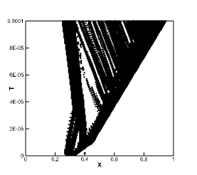
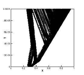
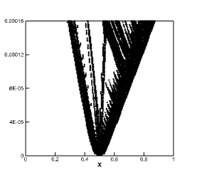
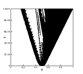
Figure 3.8: The points where the WENO procedures are performed for Examples 3.4 to 3.6. From left to right: the results of Old hybrid WENO method; the results of New/simplified hybrid WENO method.

Example 3.7. This problem is a Mach 1.22 air shock acting on a helium bubble, then, we solve the governing equations (2.1) for two dimensional Euler equations, and its physical initial schematic diagram is shown in the left of Figure 3.9. The reflective conditions are applied in the upper and lower boundary, while the inflow/outflow conditions are given in the left and right boundary, respectively. The non-dimensionalized initial conditions are given as follows

$$\begin{array}[]{rll}(\rho,\mu,\nu,p,\gamma)&=&\left\{\begin{array}[]{ll}(1,0,0,1,1.4),&\text{pre-shocked air},\\ (1.3764,0.394,0,1.5698,1.4),&\text{post-shocked air},\\ (0.138,0,0,5/3),&\text{helium},\\ \end{array}\right.\\ \phi&=&\sqrt{x^{2}+y^{2}}-1,\quad\quad\quad\quad\quad\quad\quad\quad\ \text{level set},\end{array}$$

in which $\phi\leq 0$ represents helium and $\phi>0$ represents the air. In addition, the region for $x<1.2$ is the post-shocked air state.

This shock impacting on a helium bubble problem had been experimentally studied in [8], and we present our computed results for density at time $0.5$, $1.0$, $2.0$ and $4.0$ with $280\times 240$ uniform points in Figure 3.10, then, we can know the numerical results are comparable to the results given in [8], and our computation for this example stops at time $t=4.0$ before the generation of the strong re-entrant jet, which is a complex physical phenomenon, and it might need to employ quite fine meshes or adaptive refinement technique seen in [18, 35].

Then, we would give some descriptions for the numerical results. At first, a initial shock impacts on the helium bubble, then, a part of the incident shock refracts into the helium bubble, and other part of the shock reflects from the surface and backs into the air. At $t=0.5$, we can see that the initial regular shock becomes irregular having bifurcation of the shock on the bubble surface for the sound speed in helium is faster than that in air, which was also illustrated in the experimental results given in [8]. At $t=1.0$, the refracted shock inside the bubble has interacted with the rear of the bubble and enters into the air, but the incident shock just went through the top of the helium bubble, then, the whole bubble starts moving to the right. At $t=2.0$, the incident shock has gone through the whole bubble, and the shape of the bubble begins to misshape. After this, a re-entrant jet begins to form. At $t=4.0$, the re-entrant jet actually has been formed, and the interface would be instable, when the re-entrant jet becomes stronger and stronger, which would affect the rear side of the bubble and cause the bubble to collapse, and the quite fine meshes or adaptive refinement technique might be needed seen in [18, 35]. Hence, our computation stops at the non-dimensional time $t=4.0$.

Finally, we also find that the results computed by New/simplified hybrid WENO and Classical WENO methods are similar, but New/simplified hybrid WENO method saves almost 35.49% computation time as we use linear approximation directly for the governing equation, the level set function and its re-initialization in the smooth regions. In addition, we find New/simplified hybrid WENO method with the new identification skill can save 9.41% computation time than Old hybrid WENO method by calculation, meanwhile, there are only 2.84% and 2.75% points where the WENO procedures are computed in New/simplified hybrid WENO and Old hybrid methods at the final time step, respectively, and the locations of WENO reconstruction computed by the two hybrid WENO methods at the final time step are given in the top of Figure 3.12, which illustrate that the new identification skill has similar ability as the old one in Old hybrid WENO method, but New/simplified hybrid WENO method with the new one has higher efficiency, and the new one is simpler as it only needs to solve the roots of a quadratic polynomial, while the old one has to calculate the zero points of a cubic polynomial.

Figure 3.9: Physical domain for Example 3.7 (left) and Example 3.8 (right)

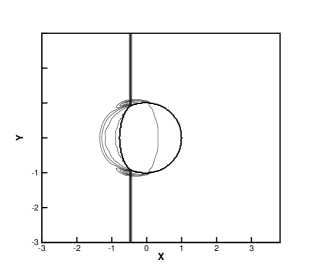
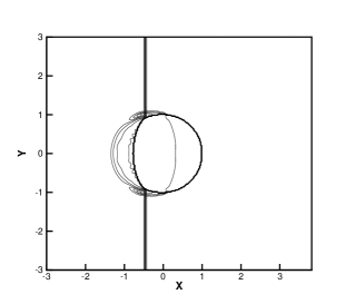
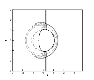
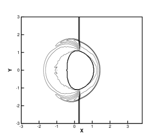
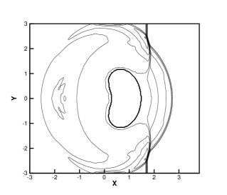
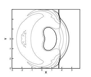
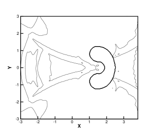
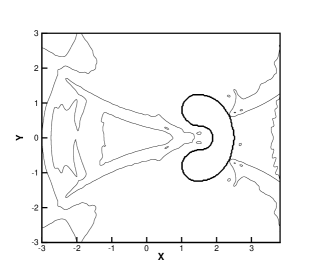
Figure 3.10: Example 3.7. The results computed by Classical WENO method (left) and New/simplified hybrid WENO method (right). 30 equally spaced density contours from 0.1 to 1.6. From top to bottom are $T=0.5$, $T=1.0$, $T=2.0$ and $T=4.0$, respectively. Grid points: $280\times 240$.

Example 3.8. The final example is a initial Mach 1.653 planar underwater shock interacting with a gas bubble in an open domain taken from [33], then we solve the governing equations (2.1) for two dimensional Euler equations with the next non-dimensionalized initial conditions:

$$\begin{array}[]{rll}(\rho,\mu,\nu,p,\gamma)&=&\left\{\begin{array}[]{ll}(1000,0,0,1,7.15),&\text{pre-shocked water},\\ (1176.3333,1.1692,0,9120,7.15),&\text{post-shocked water},\\ (1,0,0,1.4),&\text{gas},\\ \end{array}\right.\\ \phi&=&\sqrt{x^{2}+y^{2}}-1,\quad\quad\quad\quad\quad\quad\quad\quad\ \text{level set},\end{array}$$

where $\phi\leq 0$ represents gas and $\phi>0$ represents the water. In addition, the region for $x<1.2$ is the post-shocked water state. The physical initial schematic diagram is given in the right of Figure 3.9. Reflective boundary conditions are applied in the upper and lower boundary. In flow and out flow boundary conditions are given in the left and right boundary, respectively. We present the computed density at $t=0.06$, $t=0.19$, $t=0.357$ and $=0.481$. The detailed physical analysis can be seen in [27] for the earlier stage, while for the late time, one can be found in [31]. Our numerical results are similar with the computed results by Qiu et al. [33], where they solved this problem by the discontinuous Galerkin finite element methods with MGFM. Again, our computation stops at time $=0.481$ before the form of the strong re-entrant jet, and the bubble doesn’t collapse at this time.

From Figure 3.11, we can see that the density computed by New/simplified hybrid WENO and Classical WENO methods are similar, however, New/simplified hybrid WENO method has higher efficiency than Classical WENO scheme for saving almost 27.13% computation time. In addition, we find New/simplified hybrid WENO method with the new identification skill can save 12.00% CPU time than the old one in Old hybrid WENO method by calculation, meanwhile, there are only 19.05% and 19.21% points where the WENO procedures are computed in the two hybrid WENO methods at the final time step, respectively, and the locations of WENO reconstruction at the final time step are shown in the bottom of Figure 3.12, which illustrate that the new identification skill in New/simplified hybrid WENO method can identify the regions of the extreme points as the old one in Old hybrid WENO, but New/simplified hybrid WENO method with the new one has higher efficiency, and the new one has simpler implementation procedure.

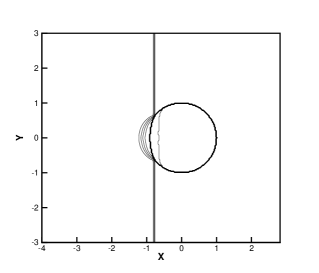
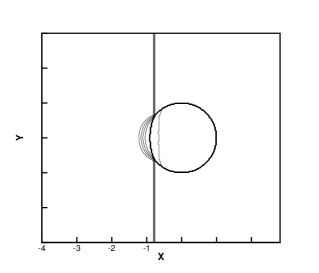
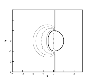
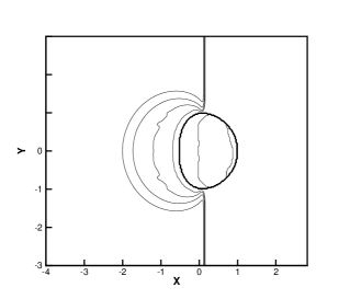
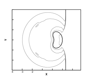
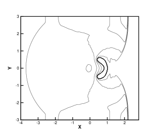
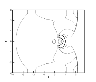
Figure 3.11: Example 3.8. The results computed by Classical WENO method (left) and New/simplified hybrid WENO method (right). 30 equally spaced density contours from 1.0 to 1200. From top to bottom are $t=0.06$, $t=0.19$, $t=0.357$ and $t=0.481$, respectively. Grid points: $280\times 240$.

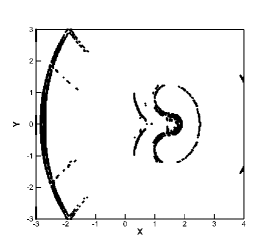
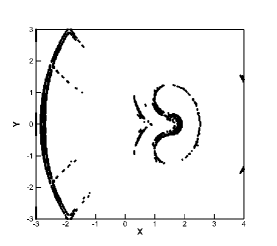
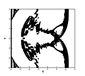
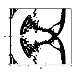
Figure 3.12: The points where the WENO procedures are performed at the final time step for Examples 3.7 and 3.8. From left to right: the results of Old hybrid WENO method; the results of New/simplified hybrid WENO method.

4 Concluding remarks

In this paper, we combine the new simplified hybrid WENO method with the modified ghost fluid method [28] to simulate the compressible two-medium flow problems, which adapts between the linear upwind approximation and WENO reconstruction automatically in terms of the regions of the extreme points for the big reconstruction polynomial, and we have an improvement about the identification technique for the regions of the extreme points of the big reconstruction polynomial. This new switch principle is not only simple for we doesn’t need to adjust the parameters, but also it is effective as we just need to know the range of the extreme point for the big reconstruction polynomial, rather than solving the exact location of the extreme point as the old one in hybrid WENO schemes [50, 48]. Comparing with the classical WENO scheme [17], the new simplified hybrid WENO scheme is more efficient with less numerical errors in the smooth region and less computation costs, meanwhile, the new simplified hybrid WENO scheme with MGFM is robust and non-oscillatory to simulate these two-medium flow problems. In general, these numerical results all show the good performances of the new simplified hybrid WENO scheme with the modified ghost fluid method.

5 Appendix A: The finite difference hybrid WENO method for Hamilton-Jacobi equations

The next finite difference hybrid WENO method for Hamilton-Jacobi equations is mainly developed from the fifth order WENO scheme introduced by Jiang and Peng [16] to solve the Hamilton-Jacobi equations (2.7), (2.8) and (2.9) in Section 2.2.

We first consider one dimensional Hamilton-Jacobi equation

$$\left\{\begin{array}[]{ll}\phi_{t}+H(x,t,\phi,\phi_{x})=0,\\ \phi(x,0)=\phi_{0}(x).\\ \end{array}\right.$$ (5.1)

The computing domain is divided by uniform grid points $\{x_{i}\}$, and the semi-discrete form of (5.1) is

$$\frac{d\phi_{i}(t)}{dt}=-\hat{H}(x_{i},t,\phi_{i},\phi_{x_{i}}^{+},\phi_{x_{i}}^{-}),$$ (5.2)

where $\phi_{i}(t)$ is represented as $\phi(x_{i},t)$, and $\phi_{x_{i}}^{\pm}$ are linear or WENO approximations for $\frac{\partial\phi(x_{i})}{\partial x}$. $\hat{H}$ is a numerical flux to approximate $H$, and we use the Lax-Friedrichs (LF) flux here as:

$$\hat{H}(x,t,\phi,u^{+},u^{-})=H\left(x,t,\phi,\frac{u^{+}+u^{-}}{2}\right)-\alpha(u^{+},u^{-})\frac{u^{+}-u^{-}}{2},$$

where $\alpha$ is $\max_{u}|H_{1}(u)|$, where $H_{1}$ is represented as the partial derivative of $H$ with respect to $\phi_{x}$.

Next, we only introduce the reconstruction procedures for $\phi_{x_{i}}^{-}$, and the reconstruction for $\phi_{x_{i}}^{+}$ is mirror symmetric with respect to $x_{i}$ of that for $\phi_{x_{i}}^{-}$. Firstly, we can easily obtain the fourth degree polynomial $p_{0}(x)$ to approximate $\phi_{x}$ in terms of the requirements:

$$\frac{1}{\Delta x}\int_{x_{i-1+l}}^{x_{i+l}}p_{0}(x)dx=\frac{1}{\Delta x}\int_{x_{i-1+k}}^{x_{i+k}}\phi_{x}dx=\frac{\phi_{x_{i+k}}-\phi_{x_{i-1+k}}}{\Delta x},\ k=-2,...,2.$$

To increase the efficiency, if all extreme points of $p_{0}(x)$ are located outside of the big spatial stencil, $\phi_{x_{i}}^{-}$ is taken as $p_{0}(x_{i})$ directly, otherwise we would use the next classical WENO procedures [16, 17], and the method to identify the regions of the extreme points for $p_{0}(x)$ has been detailedly introduced in Section 2.2.

Now, we would give a brief review of the WENO reconstruction for $\phi_{x_{i}}^{-}$. Similarly, we obtain three quadratic polynomials $p_{l}(x)$ to approximate $\phi_{x}$, satisfying

$$\frac{1}{\Delta x}\int_{x_{i-3+k+l}}^{x_{i-2+k+l}}p_{l}(x)dx=\frac{1}{\Delta x}\int_{x_{i-3+k+l}}^{x_{i-2+k+l}}\phi_{x}dx=\frac{\phi_{x_{i-2+k+l}}-\phi_{x_{i-3+k+l}}}{\Delta x},\ k=-1,0,1,\ l=1,2,3.$$

For saving space, the explicit values of $p_{l}(x_{i})$, the linear weights $\gamma_{l}$, the smoothness indicators $\beta_{l}$, and the nonlinear weights $\omega_{l}$ are not present here, and these expressions can be seen in [16, 17]. Finally, the WENO reconstruction of $\phi^{-}_{x_{i}}$ is approximated by

$$\phi^{-}_{x_{i}}=\sum_{l=1}^{3}\omega_{l}p_{l}(x_{i}).$$

For the two dimensional Hamilton-Jacobi equation

$$\left\{\begin{array}[]{ll}\phi_{t}+H(x,y,t,\phi,\phi_{x},\phi_{y})=0,\\ \phi(x,y,0)=\phi_{0}(x,y).\\ \end{array}\right.$$ (5.3)

The computing domain is divided by uniform grid points $\{(x_{i},y_{j})\}$, and the semi-discrete form of (5.3) is

$$\frac{d\phi_{i,j}(t)}{dt}=-\hat{H}(x_{i},y_{j},t,\phi_{i,j},\phi_{x,i,j}^{+},\phi_{x,i,j}^{-},\phi_{y,i,j}^{+},\phi_{y,i,j}^{-}),$$ (5.4)

where $\phi_{i,j}(t)$ is represented as $\phi(x_{i},y_{j},t)$. $\phi_{x,i,j}^{\pm}$ and $\phi_{y,i,j}^{\pm}$ are linear or WENO approximations for $\frac{\partial\phi(x_{i},y_{j})}{\partial x}$ and $\frac{\partial\phi(x_{i},y_{j})}{\partial y}$, respectively. $\hat{H}$ is a numerical flux to approximate $H$, and we use the Lax-Friedrichs (LF) flux here as:

$$\hat{H}(x_{i},y_{j},t,\phi_{i,j},u^{+},u^{-},v^{+},v^{-})=H(x_{i},y_{j},t,\phi_{i,j},\frac{u^{+}+u^{-}}{2},\frac{v^{+}+v^{-}}{2})-\alpha\frac{u^{+}-u^{-}}{2}-\beta\frac{v^{+}-v^{-}}{2},$$

where $\alpha$ is $\max_{u}|H_{1}(u,v)|$ and $\beta$ is $\max_{v}|H_{2}(u,v)|$. $H_{1}$ and $H_{2}$ are represented as the partial derivative of $H$ with respect to $\phi_{x}$ and $\phi_{y}$, respectively. Finally, $\phi_{x,i,j}^{\pm}$ and $\phi_{y,i,j}^{\pm}$ are reconstructed by dimension by dimension as one dimension case.

For the time discretization, the semi-discrete schemes (5.2) and (5.4) are discretized by the third order Runge-Kutta method [39] in (2.6) of Section 2.2.

References

- [1] R. Abgrall, How to prevent oscillations in multicomponent flow calculations: a quasi conservative approach, J. Comput. Phys., 125 (1996), 150-160.
- [2] R. Abgrall and S. Karni, Computations of compressible multifluids, J. Comput. Phys., 169 (2001), 594-623.
- [3] M. Castro, B. Costa and W.S. Don, High order weighted essentially non-oscillatory WENO-Z schemes for hyperbolic conservation laws, J. Comput. Phys., 230 (2011), 1766-1792.
- [4] T.-J. Chen and C.H. Cooke, On the Riemann problem for liquid or gas-liquid media, Int. J. Numer. Meth. Fluids, 18 (1994), 529-541.
- [5] Y. Chen and S. Jiang, A non-oscillatory kinetic scheme for multi-component flows with equation of state for a stiffened gas, J. Comput. Math., 29 (2011), 661-683.
- [6] R. P. Fedkiw, T. Aslam, B. Merriman and S. Osher, A non-oscillatory Eulerian approach to interfaces in multimaterial flows (the ghost fluid method), J. Comput. Phys., 152 (1999), 457-492.
- [7] J. Glimm, J.W. Grove, X.L. Li, K.-M. Shyue, Y. Zheng and Q. Zhang, Three-dimensional front tracking, SIAM J. Sci. Comput., 19 (1998), 703-727.
- [8] J.-F. Haas and B. Sturtevant, Interaction of weak shock waves with cylindrical and spherical gas inhomogeneities, J. Fluid Mech., 181 (1987), 41-76.
- [9] A. Harten, Preliminary results on the extension of ENO schemes to two-dimensional problems, in Proceedings, International Conference on Nonlinear Hyperbolic Problems, Saint-Etienne, 1986, Lecture Notes in Mathematics, edited by C. Carasso et al. (Springer-Verlag, Berlin, 1987).
- [10] A. Harten, B. Engquist, S. Osher and S. Chakravarthy, Uniformly high order accurate essentially non-oscillatory schemes III, J. Comput. Phys., 71 (1987), 231-323.
- [11] A. Harten and S. Osher, Uniformly high-order accurate non-oscillatory schemes, IMRC Technical Summary Rept. 2823, Univ. of Wisconsin, Madison, WI, May 1985.
- [12] D.J. Hill and D.I. Pullin, Hybrid tuned center-difference-WENO method for large eddy simulations in the presence of strong shocks, J. Comput. Phys., 194 (2004), 435-450.
- [13] C. Hirt and B. Nichols, Volume of fluid (VOF) method for the dynamics of free boundaries, J. Comput. Phys., 39 (1981), 201-225.
- [14] X.Y. Hu and B.C. Khoo, An interface interaction method for compressible multifluids, J. Comput. Phys., 198 (2004), 35-64.
- [15] C. Hu and C.-W. Shu, Weighted essentially non-oscillatory schemes on triangular meshes, J. Comput. Phys., 150 (1999), 97-127.
- [16] G.-S. Jiang and D. Peng, Weighted ENO schemes for Hamilton-Jacobi equations, SIAM J. Sci. Comput., 21 (2000), 2126-2143.
- [17] G.-S. Jiang and C.-W. Shu, Efficient implementation of weighted ENO schemes, J. Comput. Phys., 126 (1996), 202-228.
- [18] E. Johnsen and T. Colonius, Implementation of WENO schemes in compressible multicomponent flow problems, J. Comput. Phys., 219 (2006), 715-732.
- [19] S. Karni, Multicomponent flow calculations by a consistent primitive algorithm, J. Comput. Phys., 112 (1994), 31-43.
- [20] B. Larrouturou, How to preserve the mass fractions positivity when computing compressible multicomponent flows, J. Comput. Phys., 95 (1991), 59-84.
- [21] D. Levy, G. Puppo and G. Russo, Central WENO schemes for hyperbolic systems of conservation laws, Math. Model. Numer. Anal., 33 (1999), 547-571.
- [22] G. Li and J. Qiu, Hybrid weighted essentially non-oscillatory schemes with different indicators, J. Comput. Phys., 229 (2010), 8105-8129.
- [23] T.G. Liu, C.L. Feng and L. Xu, Modified Ghost Fluid Method with Acceleration Correction (MGFM/AC), J. Sci. Comput., 81 (2019), 1906-1944.
- [24] T.G. Liu and B.C. Khoo, The accuracy of the modified ghost fluid method for gas-gas Riemann problem, Adv. Appl. Math., 57 (2007), 721-733.
- [25] T.G. Liu, B.C. Khoo and W.F. Xie, The modified ghost fluid method as applied to extreme fluid-structure interaction in the presence of cavitation, Commun. Comput. Phys., 1 (2006), 898-919.
- [26] T. G. Liu, B. C. Khoo and K. S. Yeo, The simulation of compressible multi-medium flow. Part I: a new methodology with applications to 1D gas-gas and gas-water cases, Comput. Fluids, 30 (2001), 291-314.
- [27] T.G. Liu, B.C. Khoo and K.S. Yeo, The simulation of compressible multi-medium flow. Part II: applications to 2D underwater shock refraction, Comput. Fluids, 30 (2001), 315-337.
- [28] T.G. Liu, B.C. Khoo and K.S. Yeo, Ghost fluid method for strong shock impacting on material interface, J. Comput. Phys., 190 (2003), 651-681.
- [29] X.D. Liu, S. Osher and T. Chan, Weighted essentially non-oscillatory schemes, J. Comput. Phys., 115 (1994), 200-212.
- [30] T.G. Liu, W.F. Xie and B.C. Khoo, The modified ghost fluid method for coupling of fluid and structure constituted with hydro-elasto-plastic equation of state, SIAM J. Sci. Comput., 30 (2008), 1105-1130.
- [31] R.R. Nourgaliev, T.N. Dinh and T.G. Theofanous, Adaptive characteristic-based matching for compressible multifluid dynamics, J. Comput. Phys., 213 (2006), 500-529.
- [32] J. Qiu, T.G. Liu and B.C. Khoo, Runge-Kutta discontinuous Galerkin methods for compressible two-medium flow simulations: One-dimensional case, J. Comput. Phys., 222 (2007), 353-373.
- [33] J. Qiu, T.G Liu and B.C. Khoo, Simulations of compressible two-medium flow by Runge-Kutta discontinuous Galerkin methods with the ghost fluid method, Commun. Comput. Phys., 3 (2008) 479-504.
- [34] J. Qiu and C.-W. Shu, A comparison of troubled-cell indicators for Runge-Kutta discontinuous Galerkin methods using weighted essentially nonoscillatory limiters, SIAM J. Sci. Comput., 27 (2005), 995-1013.
- [35] J.J. Quirk and S. Karni, On the dynamics of a shock-bubble interaction, J. Fluid Mech., 318 (1996), 129-163.
- [36] R. Saurel and R. Abgrall, A simple method for compressible multifluid flows, SIAM J. Sci. Comput., 21 (1999), 1115-1145.
- [37] J. Shi, C. Hu and C.-W. Shu, A technique of treating negative weights in WENO schemes, J. Comput. Phys., 175 (2002), 108-127.
- [38] C.-W. Shu, High order weighted essentially nonoscillatory schemes for convection dominated problems, SIAM Review, 51 (2009), 82-126.
- [39] C.-W. Shu and S. Osher, Efficient implementation of essentially non-oscillatory shock capturing schemes, J. Comput. Phys., 77 (1988), 439-471.
- [40] K.-M. Shyue, An efficient shock-capturing algorithm for compressible multicomponent problems, J. Comput. Phys., 142 (1998), 208-242.
- [41] M. Sussman, P. Smereka and S. Osher, A level set approach for computing solutions to incompressible two-phase flow, J. Comput. Phys., 114 (1994), 146-159.
- [42] S.O. Unverdi and G. Tryggvason, A front-tracking method for viscous incompressible multi-fluid flows, J. Comput. Phys., 100 (1992), 25-37.
- [43] C.W. Wang, T.G. Liu and B.C. Khoo, A real-ghost fluid method for the simulation of multimedium compressible flow, SIAM J. Sci. Comput., 28 (2006), 278-302.
- [44] L. Xu, C.L. Feng and T.G. Liu, Practical techniques in ghost fluid method for compressible multi-medium flows, Commun. Comput. Phys., 20 (2016), 619-659.
- [45] L. Xu and T.G. Liu, Optimal error estimation of the modified ghost fluid method, Commun. Comput. Phys., 8 (2010), 403-426.
- [46] L. Xu and T.G. Liu, Modified ghost fluid method as applied to fluid Cplate interaction, Adv. Appl. Math. Mech. 6 (2014), 24-48.
- [47] Y.-T. Zhang and C.-W. Shu, Third order WENO scheme on three dimensional tetrahedral meshes, Commun. Comput. Phys., 5 (2009), 836-848.
- [48] Z. Zhao, J. Zhu, Y. Chen and J. Qiu, A new hybrid WENO scheme for hyperbolic conservation laws, Comput. Fluids, 179 (2019), 422-436.
- [49] J. Zhu and J. Qiu, A new fifth order finite difference WENO scheme for solving hyperbolic conservation laws, J. Comput. Phys., 318 (2016), 110-121.
- [50] J. Zhu and J. Qiu, A new type of modified WENO schemes for solving hyperbolic conservation laws, SIAM. J. Sci. Comput., 39 (2017), A1089-A1113.
- [51] J. Zhu and C.-W. Shu, A new type of multi-resolution WENO schemes with increasingly higher order of accuracy, J. Comput. Phys., 375 (2018), 659-683.