New method for calculating electromagnetic effects in semileptonic beta-decays of mesons

Abstract

We construct several classes of hadronic matrix elements and relate them to the low-energy constants in Chiral Perturbation Theory that describe the electromagnetic effects in the semileptonic beta decay of the pion and the kaon. We propose to calculate them using lattice QCD, and argue that such a calculation will make an immediate impact to a number of interesting topics at the precision frontier, including the outstanding anomalies in $|V_{us}|$ and the top-row Cabibbo-Kobayashi-Maskawa matrix unitarity.

I Introduction

The last few years have seen a rapid development in the theory of the electroweak radiative corrections (RCs) in hadron and nuclear beta decay processes. In particular, a dispersion relation analysis Seng:2018yzq ; Seng:2018qru significantly reduced the hadronic uncertainty of the single-particle RCs in free neutron and superallowed nuclear beta decays, and led to a new status of the top-row Cabibbo-Kobayashi-Maskawa (CKM) matrix unitarity, as quoted in the 2020 Particle Data Group (PDG) Zyla:2020zbs :

$$|V_{ud}|^{2}+|V_{us}|^{2}+|V_{ub}|^{2}=0.9985(3)_{V_{ud}}(4)_{V_{us}},$$ (1)

in contrast to the result in the 2018 PDG Tanabashi:2018oca with $0.9994(4)_{V_{ud}}(4)_{V_{us}}$ at the right hand side (RHS). The apparent violation of the top-row CKM unitarity at a 3$\sigma$ level and its implications on the possible physics Beyond the Standard Model (BSM) Gonzalez-Alonso:2018omy ; Bryman:2019ssi ; Belfatto:2019swo ; Cirgiliano:2019nyn ; Tan:2019yqp ; Bryman:2019bjg ; Grossman:2019bzp ; Coutinho:2019aiy ; Cheung:2020vqm ; Crivellin:2020lzu ; Endo:2020tkb ; Capdevila:2020rrl ; Kirk:2020wdk trigger renewed interest from both the experimental and theoretical community in the precision frontier.

The improvements in the recent years mainly concern the reduction of the Standard Model (SM) theory uncertainties in the extraction of $V_{ud}$. And now, as indicated in Eq.(1), the next breakthrough must involve a similar reduction of the $V_{us}$ theory uncertainties. In particular, the outstanding disagreement between the $V_{us}$ extracted from the kaon semileptonic decay ($K_{l3}$) and leptonic decay ($K_{l2}$) Zyla:2020zbs :

$$|V_{us}|=\left\{\begin{array}[]{c}0.2231(4)_{\mathrm{exp+RCs}}(6)_{\mathrm{lattice}}\>\>(N_{f}=2+1+1,\>K_{l3})\\ 0.2252(5)\>\>(N_{f}=2+1+1,\>K_{\mu 2})\end{array}\right.$$ (2)

has to be understood. Apart from possible BSM explanations, such a disagreement could originate either from unknown systematic errors in the SM input of the $K\pi$ form factor or, although somewhat less likely, the RCs in $K_{l3}$. For the first case one simply needs a better lattice Quantum Chromodynamics (QCD) calculation of the $K\pi$ form factor at zero momentum transfer, whereas the second case is much more complicated and will be the focus in this paper. In particular, we will discuss the possible roles that lattice QCD can play in this aspect.

Recently lattice QCD has made a tremendous progress in first-principles studies of Quantum Electrodynamics (QED) corrections to hadronic processes, see e.g. Carrasco:2015xwa ; Lubicz:2016xro ; Giusti:2017dwk ; DiCarlo:2019thl . In particular, Ref. Giusti:2017dwk presented, for the first time, the full lattice study of the QED RCs to the $K_{\mu 2}$ and $\pi_{\mu 2}$ decay rates, which involves a direct calculation of both the virtual and real photon emission diagrams. The extension of the method above to semileptonic decay processes is, however, expected to be extremely challenging Giusti:2018guw ; Sachrajda:2019uhh ; Cirigliano:2019jig . On the other hand, Ref. Feng:2020zdc adopted a completely different starting point, namely to calculate the so-called “axial $\gamma W$ box diagram” on the lattice, which resulted in a significant reduction of the theory uncertainty in $\pi_{e3}$ Feng:2020zdc , and also provided an independent cross-check of the dispersion relation analysis in the neutron RCs Seng:2020wjq . This is the first time lattice QCD ever plays a decisive role in the understanding of RCs of semi-leptonic beta decays, so a natural question to ask is whether the same method is going to teach us anything useful about the RCs in $K_{l3}$, which is much more complicated than $\pi_{e3}$ due to its larger Q-value.

The answer is yes if we appropriately combine lattice QCD with the existing theory framework. We first recall that the standard approach to deal with the electroweak RCs in $K_{l3}$ is based on Chiral Perturbation Theory (ChPT) Cirigliano:2001mk ; Cirigliano:2008wn , in which the theoretical uncertainties are from two sources: (1) the neglected terms that scale as higher-order in the chiral power counting, and (2) the unknown low-energy constants (LECs). The first can in principle be reduced by including higher-order loop corrections, whereas the second represents a more fundamental issue: the LECs characterize the unknown dynamics of QCD at the chiral symmetry breaking scale $\Lambda_{\chi}\sim 1$ GeV. The LECs are not constrained by chiral symmetry, and there is no reliable experimental constraint on the ones that describe the electromagnetic interactions of mesons. They are so far only calculated within models Ananthanarayan:2004qk ; DescotesGenon:2005pw with no rigorous error analysis. Therefore, the ability to determine the relevant LECs with high accuracy will serve as a first step in the breakthrough of the $V_{us}$ theory.

There is also another motivation to get more reliable values of these LECs. In leptonic decay processes, one extracts $|V_{us}/V_{ud}|$ by considering the ratio $R_{A}=\Gamma_{K_{\mu 2}}/\Gamma_{\pi_{\mu 2}}$ Marciano:2004uf , because it turns out that the $K_{\mu 2}$ and $\pi_{\mu 2}$ decay rates share not only the same short-distance electroweak RCs, but also the same combination of LECs at $\mathcal{O}(e^{2}p^{2})$ so they cancel out in the ratio. This leads to a smaller theoretical uncertainty than the extractions of the individual $|V_{us}|$ and $|V_{ud}|$ themselves. Recently, a similar ratio $R_{V}=\Gamma_{K_{l3}}/\Gamma_{\pi_{e3}}$ was introduced for the semileptonic decay processes Czarnecki:2019iwz , which provides another venue to extract $|V_{us}/V_{ud}|$ and could shed new lights on the $V_{us}$ discrepancy mentioned above. However, we find that $\Gamma_{K_{l3}}$ and $\Gamma_{\pi_{e3}}$ do not share the same LECs at $\mathcal{O}(e^{2}p^{2})$ and so they do not fully cancel in the ratio. Therefore, one could better make use of $R_{V}$ if its residual dependence on the LECs can be fixed through an extra lattice QCD calculation.

In this paper we demonstrate how all the LECs relevant for the RCs in $K_{l3}$ and $\pi_{e3}$ can be pinned down by calculating two types of rather simple hadronic matrix elements on lattice. The first type is just the axial $\gamma W$ box diagram, which has already been done for pion. We derive a matching relation between this quantity and the relevant LECs, and show that the lattice QCD result differs significantly from the widely-adopted value based on resonance model estimation DescotesGenon:2005pw , which motivates us even further for a thorough re-analysis. A similar calculation of the $K_{e3}^{0}$ box diagram at the SU(3) symmetric point will eventually fix all the needed LECs that describe the lepton-hadron electromagnetic interactions. Finally, for the remaining LECs that do not involve a lepton, we propose a lattice calculation of the four-point correlation functions based on the construction in Ref. Ananthanarayan:2004qk .

The contents in this paper are arranged as follows. In Sec. II we review the existing theory frameworks to study the electroweak RCs in kaon and pion semileptonic decays, including the classical “Sirlin’s representation” and the modern ChPT representation. We show in Sec. III that comparing these two representations in the SU(3) limit gives an elegant matching relation between a subset of LECs and the axial $\gamma W$ box diagram calculable on lattice. We discuss the implications of the lattice result in Ref. Feng:2020zdc and propose a similar calculation in the $K\pi$ system. In Sec. IV we construct a class of four-point correlation functions that enable a direct lattice determination of the lepton-free LECs. Our final conclusions are given in Sec. V.

II Radiative corrections to semileptonic beta decays in two representations

We start by reviewing the existing theoretical frameworks in the treatment of the semileptonic decay of a generic spinless particle $\phi$, and its corresponding electroweak RCs. First, the electromagnetic and charged weak currents in the quark sector are defined as:

$$J_{\mathrm{em}}^{\mu}=\frac{2}{3}\bar{u}\gamma^{\mu}u-\frac{1}{3}\bar{d}\gamma^{\mu}d-\frac{1}{3}\bar{s}\gamma^{\mu}s,\>\>\>J_{W}^{\mu}=V_{ud}\bar{u}\gamma^{\mu}(1-\gamma_{5})d+V_{us}\bar{u}\gamma^{\mu}(1-\gamma_{5})s,$$ (3)

and the matrix element of the charged weak current can be expressed in terms of two form factors:

$$F^{\mu}_{fi}(p^{\prime},p)=\left\langle\phi_{f}(p^{\prime})\right|J_{W}^{\mu\dagger}(0)\left|\phi_{i}(p)\right\rangle=F_{+}^{fi}(t)(p+p^{\prime})^{\mu}+F_{-}^{fi}(t)(p-p^{\prime})^{\mu},$$ (4)

where $t=(p-p^{\prime})^{2}$. Notice that in the definition above the form factors contain the CKM matrix elements. It is useful to remember that the contribution from $F_{-}^{fi}$ to the decay rate is suppressed at tree level by the factor $m_{l}^{2}/M_{\phi_{i}}^{2}$, where $l$ is the emitted charged lepton.

Now let us consider the decay process $\phi_{i}(p)\to\phi_{f}(p^{\prime})e^{+}(p_{e})\nu_{e}(p_{\nu})$, where $\phi_{i,f}$ are spinless particles. At tree level the decay amplitude is given by:

$$M_{0}=-\frac{G_{F}}{\sqrt{2}}\bar{u}_{\nu}\gamma_{\lambda}(1-\gamma_{5})v_{e}F_{fi}^{\lambda}(p^{\prime},p)\leavevmode\nobreak\ .$$ (5)

Here, $G_{F}=1.1663787(6)\times 10^{-5}$ GeV^-2 is the Fermi constant measured in muon decay. This definition has a natural advantage as it absorbs a large portion of the electroweak RCs that is common to both the muon and hadron semileptonic beta decays into the definition of $G_{F}$.

Next we discuss the two different representations of the electroweak RCs in this decay process, namely Sirlin’s representation and the effective field theory (EFT) representation. We will show later that the comparison between the results in these two representations leads to useful relations between the LECs in ChPT and hadronic matrix elements calculable on lattice. To avoid discussing issues such as the gauge-dependence of the LECs, throughout this paper we simply adopt the Feynman gauge which is the standard choice in all papers of similar topics.

II.1 Sirlin’s representation

Earliest theory analysis of electromagnetic RCs in Fermi interactions can be traced back to the seminal work by Kinoshita and Sirlin in 1958 Kinoshita:1958ru , and later by Sirlin. He derived the universal function $g(E,E_{m},m)$ that summarizes the infrared (IR) physics of the RCs in generic beta decay processes Sirlin:1967zza . The analysis was then extended to the full electroweak RCs, where the muon decay rate was taken as a normalization Sirlin:1974ni . All these were later integrated into a complete theory framework based on current algebra Sirlin:1977sv and the on-shell renormalization of the SM electroweak sector Sirlin:1980nh , which we shall name as Sirlin’s representation. Despite being gradually superseded by the EFT representation, recently it was re-introduced in the study of $K_{l3}$ RCs in a hybridized form with EFT, which aims to further reduce the existing theory uncertainty Seng:2019lxf .

In Sirlin’s representation, the $\mathcal{O}(G_{F}\alpha)$ electroweak RCs to the amplitude of a semi-leptonic decay process of a spinless particle $\phi_{i}(p)\to\phi_{f}(p^{\prime})e^{+}(p_{e})\nu_{e}(p_{\nu})$ can be summarized as Seng:2019lxf :

$$\delta M = \left[-\frac{\alpha}{2\pi}\left(\ln\frac{M_{W}^{2}}{M_{Z}^{2}}+\frac{1}{4}\ln\frac{M_{W}^{2}}{m_{e}^{2}}-\frac{1}{2}\ln\frac{m_{e}^{2}}{M_{\gamma}^{2}}+\frac{9}{8}+\frac{3}{4}a_{\mathrm{pQCD}}\right)+\frac{1}{2}\delta_{\mathrm{HO}}^{\mathrm{QED}}\right]M_{0}$$ (6)

$$-\frac{G_{F}}{\sqrt{2}}\bar{u}_{\nu}\gamma_{\lambda}(1-\gamma_{5})v_{e}\delta F_{fi}^{\lambda}(p^{\prime},p)+\delta M_{\gamma W}\leavevmode\nobreak\ .$$

The first line in the equation above represents the contributions from the “weak” RCs (see Ref. Seng:2019lxf for rigorous definition) including its perturbative QCD (pQCD) corrections $a_{\mathrm{pQCD}}\approx 0.068$, the electromagnetic RC to the electron wavefunction renormalization (with a small photon mass $M_{\gamma}$ as an IR regulator), as well as the contribution from the resummation of the large QED logs, which is formally of higher order but numerically sizable: $\delta_{\mathrm{HO}}^{\mathrm{QED}}=0.0010(3)$ Erler:2002mv . The second line encodes the contribution from the electromagnetic RCs to the charged weak matrix element and the $\gamma W$ box diagram. Employing the on-mass-shell formula Brown:1970dd and Ward identities, the form factor correction splits into two pieces: $\delta F^{\lambda}_{fi}=\delta F^{\lambda}_{fi,2}+\delta F^{\lambda}_{fi,3}$, among which the “two-point function” contribution reads:

$$\delta F_{fi,2}^{\lambda}(p^{\prime},p)=-\frac{e^{2}}{2}\int\frac{d^{4}q^{\prime}}{(2\pi)^{4}}T^{\mu}_{fi\>\mu}(q^{\prime};p^{\prime},p)\frac{\partial}{\partial q^{\prime}_{\lambda}}\left(\frac{1}{q^{\prime 2}-M_{\gamma}^{2}}\frac{M_{W}^{2}}{M_{W}^{2}-q^{\prime 2}}\right),$$ (7)

where we have defined the “generalized Compton tensor” that consists of the interference between the electromagnetic and charged weak current as:

$$T^{\mu\nu}_{fi}(q^{\prime};p^{\prime},p)=\int d^{4}xe^{iq^{\prime}\cdot x}\left\langle\phi_{f}(p^{\prime})\right|T\{J_{\mathrm{em}}^{\mu}(x)J_{W}^{\nu\dagger}(0)\}\left|\phi_{i}(p)\right\rangle\leavevmode\nobreak\ .$$ (8)

On the other hand, the explicit form of the “three-point function” contribution $\delta F_{fi,3}^{\lambda}$ is not of our concern. One needs only to know that it vanishes when the vector charged weak current is conserved and $p-p^{\prime}=0$. Finally, the $\gamma W$ box diagram contribution is given by:

$$\delta M_{\gamma W}=-\frac{G_{F}e^{2}}{\sqrt{2}}\int\frac{d^{4}q^{\prime}}{(2\pi)^{4}}\frac{\bar{u}_{\nu}\gamma^{\nu}(1-\gamma_{5})(\not{q}^{\prime}-\not{p}_{e}+m_{e})\gamma^{\mu}v_{e}}{(p_{e}-q^{\prime})^{2}-m_{e}^{2}}\frac{1}{q^{\prime 2}-M_{\gamma}^{2}}\frac{M_{W}^{2}}{M_{W}^{2}-q^{\prime 2}}T_{\mu\nu}^{fi}(q^{\prime};p^{\prime},p)\leavevmode\nobreak\ .$$ (9)

An important point to notice is that all the integrals above are ultraviolet (UV)-finite, so there is no need to introduce any extra UV-regulators and unknown counterterms.

Further simplifications can be made to the expressions above. First, using the on-shell formula $(\not{p}_{e}+m_{e})v_{e}=0$ and the Dirac matrix identity:

$$\gamma^{\mu}\gamma^{\nu}\gamma^{\alpha}=g^{\mu\nu}\gamma^{\alpha}-g^{\mu\alpha}\gamma^{\nu}+g^{\nu\alpha}\gamma^{\mu}-i\epsilon^{\mu\nu\alpha\beta}\gamma_{\beta}\gamma_{5},$$ (10)

with $\epsilon^{0123}=-1$ in our convention, the lepton tensor in Eq.(9) can be rewritten as:

$$\bar{u}_{\nu}\gamma^{\nu}(1-\gamma_{5})(\not{q}^{\prime}-\not{p}_{e}+m_{e})\gamma^{\mu}v_{e}=\bar{u}_{\nu}\gamma_{\lambda}(1-\gamma_{5})v_{e}\left[g^{\lambda\nu}q^{\prime\mu}+g^{\lambda\mu}q^{\prime\nu}-g^{\mu\nu}q^{\prime\lambda}-2g^{\lambda\nu}p_{e}^{\mu}+i\epsilon^{\mu\nu\alpha\lambda}q_{\alpha}^{\prime}\right]\leavevmode\nobreak\ .$$ (11)

With this, the box diagram contribution in Eq. (9) splits into two parts:

$$\delta M_{\gamma W}=\delta M_{\gamma W}^{V}+\delta M_{\gamma W}^{A}\leavevmode\nobreak\ ,$$ (12)

where $\delta M_{\gamma W}^{V}$ and $\delta M_{\gamma W}^{A}$ include the contribution from the first four terms and the last term at the RHS of Eq.(11), respectively.

Next, we recall that the generalized Compton tensor satisfies the following Ward identities:

$$q_{\mu}^{\prime}T^{\mu\nu}_{fi}(q^{\prime};p^{\prime},p) = -iF^{\nu}_{fi}(p^{\prime},p)$$

$$q_{\nu}T^{\mu\nu}_{fi}(q^{\prime};p^{\prime},p) = -iF^{\mu}_{fi}(p^{\prime},p)-i\Gamma^{\mu}_{fi}(q^{\prime};p^{\prime},p)\leavevmode\nobreak\ ,$$ (13)

where $q=p^{\prime}+q^{\prime}-p$, and

$$\Gamma^{\mu}_{fi}(q^{\prime};p^{\prime},p)=\int d^{4}xe^{iq^{\prime}\cdot x}\left\langle\phi_{f}(p^{\prime})\right|T\{J_{\mathrm{em}}^{\mu}(x)\partial\cdot J_{W}^{\dagger}(0)\}\left|\phi_{i}(p)\right\rangle\leavevmode\nobreak\ .$$ (14)

These Ward identities are derived from the equal-time commutation relation between the $J_{W}^{0\dagger}$ and $J_{\mathrm{em}}^{\mu}$, i.e. the current algebra relation, which is protected from perturbative Quantum Chromodynamics (pQCD) corrections to all orders.

With the identities above, the two-point function contribution (i.e. Eq.(7)) and $\delta M_{\gamma W}^{V}$ sums up to give:

$$\delta M_{2}+\delta M_{\gamma W}^{V} = \frac{\alpha}{2\pi}\left[\ln\frac{M_{W}^{2}}{m_{e}^{2}}+\frac{3}{4}+\frac{1}{2}\tilde{a}_{g}^{\mathrm{res}}\right]M_{0}+\frac{G_{F}e^{2}}{\sqrt{2}}\bar{u}_{\nu}\gamma_{\lambda}(1-\gamma_{5})v_{e}\int\frac{d^{4}q^{\prime}}{(2\pi)^{4}}\frac{M_{W}^{2}}{M_{W}^{2}-q^{\prime 2}}$$ (15)

$$\times\frac{1}{(p_{e}-q^{\prime})^{2}-m_{e}^{2}}\left\{\frac{2p_{e}\cdot q^{\prime}q^{\prime\lambda}}{(q^{\prime 2}-M_{\gamma}^{2})^{2}}T^{\mu}_{fi\>\mu}(q^{\prime};p^{\prime},p)+\frac{2p_{e\mu}}{q^{\prime 2}-M_{\gamma}^{2}}T^{\mu\lambda}_{fi}(q^{\prime};p^{\prime},p)\right.$$

$$\left.-\frac{(p-p^{\prime})_{\mu}}{q^{\prime 2}-M_{\gamma}^{2}}T^{\lambda\mu}_{fi}(q^{\prime};p^{\prime},p)+\frac{i}{q^{\prime 2}-M_{\gamma}^{2}}\Gamma^{\lambda}_{fi}(q^{\prime};p^{\prime},p)\right\}\leavevmode\nobreak\ .$$

Here, $\tilde{a}_{g}^{\mathrm{res}}\approx 0.019$ is a small pQCD correction to the two-point function. Using the free-field operator product expansion (OPE) of the hadronic tensors, it is easy to see that the remaining integrals in the equation above do not depend on physics at the scale $q^{\prime}\sim M_{W}$.

II.2 The EFT representation

The second and more commonly adopted representation in studies of the RCs in beta decays is based on the EFT of the SM at low energy. In such a formalism, one constructs the most general Lagrangian consistent with the symmetry properties of the underlying theory in terms of the relevant low-energy degrees of freedom (DOFs). UV-divergences due to loop integrals are first regularized using dimensional regularization (DR) and then canceled by the corresponding LECs. A power counting scheme is defined to ensure the finiteness of terms in the Lagrangian for any given precision that one wants to achieve. Finally, a matching with the perturbative calculation in the SM at the UV-end is carried out to determine the dependence of the LECs on the UV-physics, e.g. large electroweak logarithms.

For the decay processes we are discussing in this paper, i.e. $K_{l3}$ and $\pi_{e3}$, the corresponding EFT is simply the three-flavor ChPT with dynamical photons and leptons. Here we shall simply quote the involved chiral Lagrangian for future reference. First, the pseudo-Nambu-Goldstone boson (pNGB) octet is contained in the usual matrix $U$. To describe its coupling with the dynamical photon field $\mathcal{A}_{\mu}$, we introduce the following covariant derivative:

$$D_{\mu}U=\partial_{\mu}U-i(r_{\mu}+q_{R}\mathcal{A}_{\mu})U+iU(l_{\mu}+q_{L}\mathcal{A}_{\mu})\leavevmode\nobreak\ ,$$ (16)

where we have introduced the left/right-handed external sources $\{l_{\mu},r_{\mu}\}$ and spurion fields $\{q_{L},q_{R}\}$ that are traceless, Hermitian matrices in the quark flavor space. We also define $u=\sqrt{U}$, and

$$u_{\mu}=i[u^{\dagger}(\partial_{\mu}-ir_{\mu}-iq_{R}\mathcal{A}_{\mu})u-u(\partial_{\mu}-il_{\mu}-iq_{L}\mathcal{A}_{\mu})u^{\dagger}]\leavevmode\nobreak\ ,$$ (17)

as well as the covariant derivatives on the spurion fields:

$$\nabla_{\mu}q_{R}=\partial_{\mu}q_{R}-i[r_{\mu},q_{R}],\>\>\>\nabla_{\mu}q_{L}=\partial_{\mu}q_{L}-i[l_{\mu},q_{L}]\leavevmode\nobreak\ .$$ (18)

Finally, for the SM charged weak interaction Lagrangian, the external sources should be identified as:

$$q_{R}=q_{L}=-eQ^{\mathrm{em}},\>\>l_{\mu}=\sum_{l}(\bar{l}\gamma_{\mu}\nu_{lL}Q_{\mathrm{L}}^{\mathrm{w}}+h.c.),\>\>r_{\mu}=0\leavevmode\nobreak\ ,$$ (19)

where

$$Q^{\mathrm{em}}=\left(\begin{array}[]{ccc}2/3&0&0\\ 0&-1/3&0\\ 0&0&-1/3\end{array}\right),\>\>Q_{\mathrm{L}}^{\mathrm{w}}=-2\sqrt{2}G_{F}\left(\begin{array}[]{ccc}0&V_{ud}&V_{us}\\ 0&0&0\\ 0&0&0\end{array}\right)\leavevmode\nobreak\ .$$ (20)

One sees that the dynamical leptons enter through the left-handed source field $l_{\mu}$.

Now we can write down the chiral Lagrangian. In a consistent chiral power counting scheme, $p$ (a typical small momentum of the pNGBs) and $e$ should carry the same chiral order. Therefore at leading order (LO) we have:

$$\mathcal{L}^{(2)} = \frac{F_{0}^{2}}{4}\left\langle D_{\mu}U(D^{\mu}U)^{\dagger}+U\chi^{\dagger}+\chi U^{\dagger}\right\rangle+ZF_{0}^{4}\left\langle q_{L}U^{\dagger}q_{R}U\right\rangle-\frac{1}{4}F_{\mu\nu}F^{\mu\nu}-\frac{1}{2\xi}(\partial_{\mu}\mathcal{A}^{\mu})^{2}$$ (21)

$$+\frac{1}{2}M_{\gamma}^{2}\mathcal{A}_{\mu}\mathcal{A}^{\mu}+\sum_{l}[\bar{l}(i\not{\partial}+e\not{\mathcal{A}}-m_{l})l+\bar{\nu}_{lL}i\not{\partial}\nu_{iL}]\leavevmode\nobreak\ ,$$

where $F_{0}$ is the pion decay constant in the chiral limit, $F_{\mu\nu}$ is the photon field strength tensor, $\chi=2B_{0}M_{q}$ with $M_{q}$ the quark mass matrix, and $Z\approx 0.8$ is obtained from the $\pi^{\pm}-\pi^{0}$ mass splitting. The notation $\left\langle...\right\rangle$ represents the trace over the flavor space. As stated above, throughout this work we choose $\xi=1$, the Feynman gauge.

To absorb the UV-divergences generated from $\mathcal{L}^{(2)}$ at one loop, one needs to introduce the next-to-leading order (NLO) chiral Lagrangian, which could either scale as $\mathcal{O}(p^{4})$ or $\mathcal{O}(e^{2}p^{2})$. The former is just the standard Gasser-Leutwyler Lagrangian Gasser:1984gg so we shall concentrate on the latter. There are two types of chiral Lagrangian at $\mathcal{O}(e^{2}p^{2})$. The first type characterizes the short-distance electromagnetic effects of hadrons Urech:1994hd ; Neufeld:1995mu :

$$\mathcal{L}^{e^{2}p^{2}}_{\{K\}} = F_{0}^{2}\left\{\frac{1}{2}K_{1}\left\langle D^{\mu}U(D_{\mu}U)^{\dagger}\right\rangle\left\langle q_{R}q_{R}+q_{L}q_{L}\right\rangle+K_{2}\left\langle D^{\mu}U(D_{\mu}U)^{\dagger}\right\rangle\left\langle q_{R}Uq_{L}U^{\dagger}\right\rangle\right.$$ (22)

$$+K_{3}\left(\left\langle(D^{\mu}U)^{\dagger}q_{R}U\right\rangle\left\langle(D_{\mu}U)^{\dagger}q_{R}U\right\rangle+\left\langle D^{\mu}Uq_{L}U^{\dagger}\right\rangle\left\langle D_{\mu}Uq_{L}U^{\dagger}\right\rangle\right)$$

$$K_{4}\left\langle(D^{\mu}U)^{\dagger}q_{R}U\right\rangle\left\langle D_{\mu}Uq_{L}U^{\dagger}\right\rangle+K_{5}\left\langle q_{L}q_{L}(D^{\mu}U)^{\dagger}D_{\mu}U+q_{R}q_{R}D^{\mu}U(D_{\mu}U)^{\dagger}\right\rangle$$

$$+K_{6}\left\langle(D^{\mu}U)^{\dagger}D_{\mu}Uq_{L}U^{\dagger}q_{R}U+D^{\mu}U(D_{\mu}U)^{\dagger}q_{R}Uq_{L}U^{\dagger}\right\rangle$$

$$+\frac{1}{2}K_{7}\left\langle\chi^{\dagger}U+U^{\dagger}\chi\right\rangle\left\langle q_{R}q_{R}+q_{L}q_{L}\right\rangle+K_{8}\left\langle\chi^{\dagger}U+U^{\dagger}\chi\right\rangle\left\langle q_{R}Uq_{L}U^{\dagger}\right\rangle$$

$$+K_{9}\left\langle(\chi^{\dagger}U+U^{\dagger}\chi)q_{L}q_{L}+(\chi U^{\dagger}+U\chi^{\dagger})q_{R}q_{R}\right\rangle$$

$$+K_{10}\left\langle(\chi^{\dagger}U+U^{\dagger}\chi)q_{L}U^{\dagger}q_{R}U+(\chi U^{\dagger}+U\chi^{\dagger})q_{R}Uq_{L}U^{\dagger}\right\rangle$$

$$+K_{11}\left\langle(\chi^{\dagger}U-U^{\dagger}\chi)q_{L}U^{\dagger}q_{R}U+(\chi U^{\dagger}-U\chi^{\dagger})q_{R}Uq_{L}U^{\dagger}\right\rangle$$

$$+K_{12}\left\langle(D^{\mu}U)^{\dagger}[\nabla_{\mu}q_{R},q_{R}]U+D^{\mu}U[\nabla_{\mu}q_{L},q_{L}]U^{\dagger}\right\rangle$$

$$\bigl{.}+K_{13}\left\langle\nabla^{\mu}q_{R}U\nabla_{\mu}q_{L}U^{\dagger}\right\rangle+K_{14}\left\langle\nabla^{\mu}q_{R}\nabla_{\mu}q_{R}+\nabla^{\mu}q_{L}\nabla_{\mu}q_{L}\right\rangle\biggr{\}},$$

although the lepton fields may still enter through the covariant derivatives. The second type involves explicit leptonic degrees of freedom. The part relevant to $K_{l3}$ and $\pi_{e3}$ RCs is given by Knecht:1999ag :

$$\mathcal{L}^{e^{2}p^{2}}_{\{X\}} = e^{2}F_{0}^{2}\sum_{l}\left\{X_{1}\bar{l}\gamma_{\mu}\nu_{lL}\left\langle u^{\mu}\left\{\mathcal{Q}_{\mathrm{R}}^{\mathrm{em}},\mathcal{Q}_{\mathrm{L}}^{\mathrm{w}}\right\}\right\rangle+X_{2}\bar{l}\gamma_{\mu}\nu_{lL}\left\langle u^{\mu}\left[\mathcal{Q}_{\mathrm{R}}^{\mathrm{em}},\mathcal{Q}_{\mathrm{L}}^{\mathrm{w}}\right]\right\rangle\right.$$ (23)

$$\left.+X_{3}m_{l}\bar{l}v_{lL}\left\langle\mathcal{Q}_{\mathrm{L}}^{\mathrm{w}}\mathcal{Q}^{\mathrm{em}}_{\mathrm{R}}\right\rangle+h.c.\right\}+e^{2}\sum_{l}X_{6}\bar{l}(i\not{\partial}+e\not{\mathcal{A}})l\leavevmode\nobreak\ ,$$

where $\mathcal{Q}_{\mathrm{R}}^{\mathrm{em}}=u^{\dagger}Q^{\mathrm{em}}u$ and $\mathcal{Q}_{\mathrm{L}}^{\mathrm{w}}=uQ_{\mathrm{L}}^{\mathrm{w}}u^{\dagger}$.

The LECs $\{K_{i},X_{i}\}$ are generically UV-divergent, and their corresponding renormalized LECs are defined as:

$$K_{i}^{r}(\mu)=K_{i}-\Sigma_{i}\lambda,\>\>\>X_{i}^{r}(\mu)=X_{i}-\Xi_{i}\lambda,$$ (24)

where

$$\lambda=\frac{\mu^{d-4}}{16\pi^{2}}\left(\frac{1}{d-4}-\frac{1}{2}\left[\ln 4\pi-\gamma_{E}+1\right]\right),$$ (25)

with $\mu$ the scale introduced in DR, $d$ the number of the space-time dimensions, and $\gamma_{E}$ the Euler-Mascheroni constant. The values of $\{\Sigma_{i},\Xi_{i}\}$ are given in Refs. Urech:1994hd ; Knecht:1999ag , respectively. In connection with the SM electroweak sector, we find that $X_{6}^{r}$ and $K_{12}^{r}$ are sensitive to physics at the scale $q\sim M_{W}$ (in another word, they carry the large electroweak logarithms). It is customary to define the combination $X_{6}^{\mathrm{phys}}(\mu)\equiv X_{6}^{r}(\mu)-4K_{12}^{r}(\mu)$ and take $\mu=M_{\rho}$ in the numerical analysis.

	$\delta_{\mathrm{em}}^{Kl}$(%)
$K_{e3}^{0}$	$0.99\pm 0.19_{e^{2}p^{4}}\pm 0.11_{\mathrm{LEC}}$
$K_{e3}^{\pm}$	$0.10\pm 0.19_{e^{2}p^{4}}\pm 0.16_{\mathrm{LEC}}$
$K_{\mu 3}^{0}$	$1.40\pm 0.19_{e^{2}p^{4}}\pm 0.11_{\mathrm{LEC}}$
$K_{\mu 3}^{\pm}$	$0.016\pm 0.19_{e^{2}p^{4}}\pm 0.16_{\mathrm{LEC}}$

Table 1: $\delta_{\mathrm{em}}^{Kl}$ calculated in ChPT Cirigliano:2008wn .

With the effective Lagrangian above, the RCs to $K_{l3}$ and $\pi_{e3}$ were computed to $\mathcal{O}(e^{2}p^{2})$ Cirigliano:2001mk ; Cirigliano:2002ng ; Cirigliano:2008wn , and we shall briefly discuss the main results. First, the master formula of the $K_{l3}$ decay rate is given by:

$$\Gamma_{K_{l3}}=\frac{C_{K}^{2}G_{F}^{2}M_{K}^{5}}{128\pi^{3}}S_{\mathrm{EW}}|F_{+}^{\pi^{-}K^{0}}(0)|^{2}I_{Kl}^{(0)}(\lambda_{i})\left(1+\delta_{\mathrm{em}}^{Kl}+\delta_{\mathrm{SU(2)}}^{K\pi}\right)\leavevmode\nobreak\ ,$$ (26)

among which the short-distance electroweak factor $S_{\mathrm{EW}}$ is defined as:

$$S_{\mathrm{EW}}\equiv 1-e^{2}\left[-\frac{1}{2\pi^{2}}\ln\frac{M_{Z}}{M_{\rho}}+(X_{6}^{\mathrm{phys}})_{\alpha_{s}}\right]+\delta_{\mathrm{HO}}^{\mathrm{QED}}=1.0229(3)\leavevmode\nobreak\ ,$$ (27)

where we take $M_{\rho}=0.77$ GeV. Here $(X_{6})^{\mathrm{phys}}_{\alpha_{s}}\approx 3.0\times 10^{-3}$ DescotesGenon:2005pw summarizes the $\mathcal{O}(\alpha_{s})$ pQCD contribution to $X_{6}^{\mathrm{phys}}$ (but not from higher-order contributions such as $\mathcal{O}(\alpha_{s}^{(2)})$, which we shall discuss later). This value is consistent with that quoted in Ref. Cirigliano:2003yr as well as the more commonly cited value of 1.0232 by Marciano and Sirlin Marciano:1993sh . Meanwhile, the long-distance EM correction is represented by the quantity $\delta_{\mathrm{em}}^{Kl}$. The ChPT estimations of their numerical values in different channels are summarized in Tab. 1. We see that there are two sources of uncertainties in $\delta_{\mathrm{em}}^{Kl}$, namely (1) the neglected higher-order terms in the chiral power counting, and (2) the LECs $\{K_{i}^{r},X_{i}^{r}\}$. Here we are only interested in its dependence on the non-unsuppressed LECs (i.e. those contributing to $\delta F_{+}^{\pi K}$):

$$\delta_{\mathrm{em}}^{K^{\pm}l} = 2e^{2}\left[-\frac{8}{3}X_{1}-\frac{1}{2}\tilde{X}_{6}^{\mathrm{phys}}(M_{\rho})-2K_{3}^{r}(M_{\rho})+K_{4}^{r}(M_{\rho})+\frac{2}{3}K_{5}^{r}(M_{\rho})+\frac{2}{3}K_{6}^{r}(M_{\rho})\right]+...,$$

$$\delta_{\mathrm{em}}^{K^{0}l} = 2e^{2}\left[\frac{4}{3}X_{1}-\frac{1}{2}\tilde{X}_{6}^{\mathrm{phys}}(M_{\rho})\right]+...,$$ (28)

where $\tilde{X}_{6}^{\mathrm{phys}}(M_{\rho})\equiv X_{6}^{\mathrm{phys}}(M_{\rho})+(2\pi^{2})^{-1}\ln(M_{Z}/M_{\rho})-(X_{6}^{\mathrm{phys}})_{\alpha_{s}}$ removes the large electroweak logarithm and the $\mathcal{O}(\alpha_{s})$ pQCD correction from $X_{6}^{\mathrm{phys}}$. As a comparison, we can define a similar quantity for $\pi_{e3}$, and its LEC-dependence reads:

$$\delta_{\mathrm{em}}^{\pi^{\pm}e}=2e^{2}\left[-\frac{2}{3}X_{1}-\frac{1}{2}\tilde{X}_{6}^{\mathrm{phys}}(M_{\rho})\right]+...\ .$$ (29)

It is useful to contrast the results above with the case of the kaon and pion leptonic beta decay. We notice that both the $K_{l2}$ and $\pi_{l2}$ decay rate depend on the same combination of LECs Knecht:1999ag :

$$E^{r}\equiv\frac{8}{3}K_{1}^{r}+\frac{8}{3}K_{2}^{r}+\frac{20}{9}K_{5}^{r}+\frac{20}{9}K_{6}^{r}-\frac{4}{3}X_{1}-4X_{2}^{r}+4X_{3}^{r}-X_{6}^{\mathrm{phys}},$$ (30)

so it will be canceled out in the ratio $R_{A}=\Gamma_{K_{\mu 2}}/\Gamma_{\pi_{\mu 2}}$, which results in a reduced theory uncertainty in the extraction of the ratio $|V_{us}/V_{ud}|$. This is, however, not the case in the ratio $R_{V}=\Gamma_{K_{l3}}/\Gamma_{\pi_{e3}}$ recently introduced in Ref. Czarnecki:2019iwz , as we see that Eqs. (28) and (29) are not identical (except the $\tilde{X}_{6}^{\mathrm{phys}}$ term which is common to all channels). Therefore, to reduce the theoretical uncertainty in $R_{V}$ we propose a first-principles calculation of $X_{1}$ and $-2K_{3}^{r}+K_{4}^{r}+(2/3)(K_{5}^{r}+K_{6}^{r})$ and outline an appropriate method below.

III Lattice QCD calculation of $X_{1}$ and $X_{6}^{\mathrm{phys}}$ via the $\gamma W$ box

We start by discussing the LECs $X_{1}$ and $X_{6}^{\mathrm{phys}}$. They describe the electromagnetic interaction between leptons and pNGBs, so it is natural to expect that they could be related to the hadronic matrix element that occurs in the $\gamma W$ box diagram, Eq. (9). This section serves to derive such a relation.

We first consider the electroweak RCs in the decay process $\phi_{i}\rightarrow\phi_{f}e^{+}\nu_{e}$ in Sirlin’s representation, and restrict ourselves to the case where $M_{\phi_{i}}\approx M_{\phi_{f}}\gg m_{e}$. In this limit, we can define a power counting where $p-p^{\prime}$, $p_{e}$ and $p_{\nu}$ all scale as a small expansion parameter $\Delta$. An enormous amount of simplification is observed if we retain the terms in $\delta M$ only up to $\mathcal{O}(\Delta^{0})$:

1. The three-point function contribution to $\delta F_{fi}^{\mu}$ vanishes;

2. The weak axial charged-current contribution to the integrals in Eq. (15) vanishes. The vector contribution does not vanish, but it survives only in the region where $q^{\prime}\sim\Delta$, so it is sufficient to replace $T^{\mu\nu}_{fi}$ and $\Gamma_{fi}^{\mu}$ by their respective “convection terms” Meister:1963zz that describe the IR behavior of these quantities. By doing so, the integrals in Eq. (15) are analytically calculable.

3. The remainder of the $\gamma W$ box contribution simplifies to $\delta M_{\gamma W}^{A}=\Box_{\gamma W}^{VA}(\phi_{f},\phi_{i})M_{0}$, where

   $$\Box_{\gamma W}^{VA}(\phi_{f},\phi_{i})\equiv\frac{ie^{2}}{2M_{\phi_{i}}^{2}}\int\frac{d^{4}q}{(2\pi)^{4}}\frac{1}{(q^{2})^{2}}\frac{M_{W}^{2}}{M_{W}^{2}-q^{2}}\epsilon^{\mu\nu\alpha\beta}q_{\alpha}p_{\beta}\frac{T_{\mu\nu}^{fi}(q;p,p)}{F_{+}^{fi}(0)}$$ (31)

   shall be denoted as the “forward axial $\gamma W$ box”, as it probes the axial charged weak current in $T_{\mu\nu}^{fi}$.

From the above, we see that in the $\Delta\to 0$ limit the only unknown piece in $\delta M$ is $\Box_{\gamma W}^{VA}(\phi_{f},\phi_{i})$ which depends on the details of the non-perturbative QCD at the hadron scale. It is, however, a well-defined hadronic matrix element which is calculable on lattice. In fact, Ref.Feng:2020zdc presented a first-principles calculation of $\Box_{\gamma W}^{VA}(\pi^{0},\pi^{+})$ by combining the direct computation of the relevant four-point contraction diagrams at small $Q^{2}=-q^{2}$ and a pQCD calculation to $\mathcal{O}(\alpha_{s}^{4})$ at large $Q^{2}$, achieving an impressive 1% overall accuracy. Other possible methods include the application of the Feynman-Hellmann theorem on lattice Seng:2019plg ; Bouchard:2016heu ; Chambers:2017dov .

Now it is clear how one could obtained the LECs $X_{1}$ and $X_{6}^{\mathrm{phys}}$ on the lattice: One repeats the calculation of $\delta M$ in the ChPT and take the $\Delta\to 0$ limit, in which the only quantities that are not determined a priori are the LECs. Therefore, comparing the expression of $\delta M$ in the $\Delta\to 0$ limit between Sirlin’s representation and the ChPT representation gives us a relation between $\{X_{1},X_{6}^{\mathrm{phys}}\}$ and $\Box_{\gamma W}^{VA}$. Of course, one needs to calculate the latter at least in two different channels to fix $X_{1}$ and $X_{6}^{\mathrm{phys}}$ individually. In what follows we choose $\pi_{e3}$ and $K_{e3}^{0}$ to fulfill this task.

III.1 Axial $\gamma W$ box diagram in $\pi_{e3}$ decay

In the $\pi_{e3}$ channel, since the strong isospin breaking effects are small, the $\Delta\to 0$ limit is in fact quite well-satisfied in nature (the same holds for the free neutron and nuclear beta decays). To evaluate the integrals in Eq. (15), we replace $T^{\mu\nu}$ and $\Gamma^{\mu}$ by their convection terms:

$$T_{\pi^{0}\pi^{+}}^{\mu\nu}(q^{\prime};p^{\prime},p) \rightarrow \frac{i(2p-q^{\prime})^{\mu}F_{\pi^{0}\pi^{+}}^{\nu}(p^{\prime},p)}{(p-q^{\prime})^{2}-M_{\pi}^{2}}$$

$$\Gamma_{\pi^{0}\pi^{+}}^{\mu}(q^{\prime};p^{\prime},p) \rightarrow -\frac{(2p-q^{\prime})^{\mu}(p^{\prime}-p)\cdot F_{\pi^{0}\pi^{+}}(p^{\prime},p)}{(p-q^{\prime})^{2}-M_{\pi}^{2}}\leavevmode\nobreak\ .$$ (32)

With these, the total one-loop electroweak RCs to the decay amplitude in Sirlin’s representation read ($u=(p-p_{e})^{2}$, $\beta=|\vec{p}_{e}|/E_{e}$):

$$\delta M = M_{0}\left\{\frac{\alpha}{4\pi}\left[\frac{3}{2}\ln\frac{M_{W}^{2}}{m_{e}^{2}}-2\ln\frac{M_{W}^{2}}{M_{Z}^{2}}+2\ln\frac{m_{e}^{2}}{M_{\gamma}^{2}}-\frac{11}{4}+\tilde{a}_{g}+4p_{e}\cdot pC_{0}(u,M_{\pi},m_{e})+\frac{1}{\beta}\ln\frac{1+\beta}{1-\beta}\right]\right.$$ (33)

$$\left.+\Box_{\gamma W}^{VA}(\pi_{0},\pi_{+})+\frac{1}{2}\delta_{\mathrm{HO}}^{\mathrm{QED}}\right\}+\frac{\alpha}{4\pi}\frac{G_{F}}{\sqrt{2}}\bar{u}_{\nu}\not{p}_{e}(1-\gamma_{5})v_{e}\frac{p\cdot F_{\pi^{0}\pi^{+}}}{p\cdot p_{e}}\frac{1}{\beta}\ln\frac{1+\beta}{1-\beta}+\mathcal{O}(\Delta)\leavevmode\nobreak\ .$$

Here, $\tilde{a}_{g}=-(3/2)a_{\mathrm{pQCD}}+\tilde{a}_{g}^{\mathrm{res}}\approx-0.083$ summarizes the $\mathcal{O}(\alpha_{s})$ pQCD correction to all one-loop diagrams except the axial $\gamma W$ box. Meanwhile, $C_{0}$ is the well-known IR-divergent loop function:

$$C_{0}(z,m_{1},m_{2})=\int\frac{d^{4}q}{i\pi^{2}}\frac{1}{(q^{2}-M_{\gamma}^{2}+i\epsilon)((q+p_{1})^{2}-m_{1}^{2}+i\epsilon)((q-p_{2})^{2}-m_{2}^{2}+i\epsilon)}\leavevmode\nobreak\ ,$$ (34)

with $p_{1}^{2}=m_{1}^{2}$, $p_{2}^{2}=m_{2}^{2}$ and $z=(p_{1}+p_{2})^{2}$. On the other hand, taking the $\Delta\to 0$ limit in the $\mathcal{O}(e^{2}p^{2})$ ChPT expression Cirigliano:2002ng gives:

$$\delta M = M_{0}\left\{\frac{\alpha}{4\pi}\left[-\frac{3}{2}-\frac{3}{2}\ln\frac{m_{e}^{2}}{\mu^{2}}+2\ln\frac{m_{e}^{2}}{M_{\gamma}^{2}}+4p_{e}\cdot pC_{0}(u,M_{\pi},m_{e})+\frac{1}{\beta}\ln\frac{1+\beta}{1-\beta}\right]+\frac{1}{2}\delta_{\mathrm{HO}}^{\mathrm{QED}}\right.$$

$$\left.+e^{2}\left(-\frac{2}{3}X_{1}-\frac{1}{2}X_{6}^{\mathrm{phys}}\right)\right\}+\frac{\alpha}{4\pi}\frac{G_{F}}{\sqrt{2}}\bar{u}_{\nu}\not{p}_{e}(1-\gamma_{5})v_{e}\frac{p\cdot F_{\pi^{0}\pi^{+}}}{p\cdot p_{e}}\frac{1}{\beta}\ln\frac{1+\beta}{1-\beta}+\mathcal{O}(\Delta)\leavevmode\nobreak\ .$$

We see that Eq. (33) and (LABEL:eq:pie3ChPT) agree completely in their IR behavior, which is of course expected.

We now want to equate these two expressions to obtain the relation between $X_{i}$ and $\Box_{\gamma W}^{VA}$. In doing so, we find the definition of $\tilde{X}_{6}^{\mathrm{phys}}$ to be not particularly convenient, because (1) in Ref.Feng:2020zdc the pQCD correction is evaluated up to $\mathcal{O}(\alpha_{s}^{4})$ instead of just $\mathcal{O}(\alpha_{s})$, and (2) in the first-principles evaluation of Eq. (31), one requires a smooth connection between the pQCD-corrected integrand in the asymptotic region and the non-perturbative integrand at small $Q^{2}$. Thus, the procedure to “remove the pQCD correction” becomes rather unnatural. Therefore, we choose instead to express our result in terms of

$$\bar{X}_{6}^{\mathrm{phys}}(M_{\rho})\equiv X_{6}^{\mathrm{phys}}(M_{\rho})+\frac{1}{2\pi^{2}}\ln\frac{M_{Z}}{M_{\rho}}\leavevmode\nobreak\ ,$$ (36)

that removes only the large electroweak logarithm but retains the full pQCD corrections to all orders. With this we obtain

$$\frac{4}{3}X_{1}+\bar{X}_{6}^{\mathrm{phys}}(M_{\rho})=-\frac{1}{2\pi\alpha}\left(\Box_{\gamma W}^{VA}(\pi_{0},\pi_{+})-\frac{\alpha}{8\pi}\ln\frac{M_{W}^{2}}{M_{\rho}^{2}}\right)+\frac{1}{8\pi^{2}}\left(\frac{5}{4}-\tilde{a}_{g}\right)\leavevmode\nobreak\ ,$$ (37)

which is the first central result in this paper: It matches a specific linear combination of $X_{1}$ and $\bar{X}_{6}^{\mathrm{phys}}$ to the axial $\gamma W$ box in $\pi_{e3}$ decay. We observe that in the first bracket at the right of Eq. (37), the large electroweak logarithm contribution to $\Box_{\gamma W}^{VA}$ has been subtracted out due to the use of $\bar{X}_{6}^{\mathrm{phys}}$ at the left.

Substituting the lattice QCD result $\Box_{\gamma W}^{VA}(\pi_{0},\pi_{+})=2.830(28)\times 10^{-3}$ Feng:2020zdc gives:

$$\frac{4}{3}X_{1}+\bar{X}_{6}^{\mathrm{phys}}(M_{\rho})=0.0140(6)_{\mathrm{box}}(8)_{\mathrm{ChPT}}\leavevmode\nobreak\ ,$$ (38)

where the first uncertainty comes from the box diagram, and the second is the estimated leading ChPT uncertainty that comes from the neglected $\pi^{0}-\eta$ mixing terms which scale as $M_{\pi}^{2}/(M_{\eta}^{2}-M_{\pi}^{2})\sim 6$%. It is instructive to compare the result above with that from the resonance model DescotesGenon:2005pw . There, they estimated $X_{1}=-3.7\times 10^{-3}$ and $\bar{X}_{6}^{\mathrm{phys}}=\tilde{X}_{6}^{\mathrm{phys}}+(X_{6}^{\mathrm{phys}})_{\alpha_{s}}=(10.4+3.0)\times 10^{-3}$, with no robust estimation of the theory uncertainty. That implies

$$\frac{4}{3}X_{1}+\bar{X}_{6}^{\mathrm{phys}}(M_{\rho})=0.0085,\>\>\>(\mathrm{resonance}\>\mathrm{model})$$ (39)

which is significantly below the lattice result. This suggests that a careful first-principles study of the LECs could lead to a visible change in the central values of $\delta_{\mathrm{em}}$.

III.2 Axial $\gamma W$ box diagram in $K_{e3}^{0}$ deacy

The same matching can in principle also be done on $K_{e3}^{0}$ deacy in order to determine another linear combination of $X_{1}$ and $\bar{X}_{6}^{\mathrm{phys}}$. The only extra complication is that $M_{K}$ is significantly larger than $M_{\pi}$ so the $\Delta\to 0$ limit is not satisfied in nature. Nevertheless, nothing prohibits us from considering an unphysical situation where $M_{K}\approx M_{\pi}\equiv M_{\phi}$, which is always achievable on the lattice, the well-known SU(3) limit. In this limit all the simplifications in Sirlin’s representation work again, provided that the axial $\gamma W$ box diagram for $K_{e3}^{0}$ decay is now evaluated at the SU(3) symmetric point (i.e. $m_{u}=m_{d}=m_{s}$) rather than on the physical point. Despite such an unphysical setting, the LECs extracted from this procedure can still be applied to physical processes because they are by definition independent of the quark masses.

To evaluate the integrals in Eq. (15), one again replaces $T^{\mu\nu}$ and $\Gamma^{\mu}$ by their convection terms. In this case they read:

$$T_{\pi^{-}K^{0}}^{\mu\nu}(q^{\prime};p^{\prime},p) \rightarrow -\frac{i(2p^{\prime}+q^{\prime})^{\mu}F_{\pi^{-}K^{0}}^{\nu}(p^{\prime},p)}{(p^{\prime}+q^{\prime})^{2}-M_{\phi}^{2}}\leavevmode\nobreak\ ,$$

$$\Gamma^{\mu}_{\pi^{-}K^{0}}(q^{\prime};p^{\prime},p) \rightarrow \frac{(2p^{\prime}+q^{\prime})^{\mu}(p^{\prime}-p)\cdot F_{\pi^{-}K^{0}}(p^{\prime},p)}{(p^{\prime}+q^{\prime})^{2}-M_{\phi}^{2}}\leavevmode\nobreak\ .$$ (40)

With these, the total one-loop electroweak RCs to the $K_{e3}^{0}$ decay amplitude in Sirlin’s representation with the unphysical setting reads ($s=(p^{\prime}+p_{e})^{2}$, $\beta=|\vec{p}_{e}|/E_{e}$):

$$\delta M = M_{0}\left\{\frac{\alpha}{4\pi}\left[\frac{3}{2}\ln\frac{M_{W}^{2}}{m_{e}^{2}}-2\ln\frac{M_{W}^{2}}{M_{Z}^{2}}+2\ln\frac{m_{e}^{2}}{M_{\gamma}^{2}}-\frac{11}{4}+\tilde{a}_{g}-4p_{e}\cdot p^{\prime}C_{0}(s,M_{\phi},m_{e})\right.\right.$$ (41)

$$\left.\left.-\frac{2}{\beta}\ln\left(-\sqrt{\frac{1-\beta}{1+\beta}}+i\epsilon\right)\right]+\left(\Box_{\gamma W}^{VA}(\pi^{-},K^{0})\right)_{\mathrm{SU(3)}}+\frac{1}{2}\delta_{\mathrm{HO}}^{\mathrm{QED}}\right\}$$

$$-\frac{\alpha}{2\pi}\frac{G_{F}}{\sqrt{2}}\bar{u}_{\nu}\not{p}_{e}(1-\gamma_{5})v_{e}\frac{p^{\prime}\cdot F_{\pi^{-}K^{0}}}{p^{\prime}\cdot p_{e}}\frac{1}{\beta}\ln\left(-\sqrt{\frac{1-\beta}{1+\beta}}+i\epsilon\right)+\mathcal{O}(\Delta)\leavevmode\nobreak\ .$$

Here, the subscript in $\left(\Box_{\gamma W}^{VA}(\pi^{-},K^{0})\right)_{\mathrm{SU(3)}}$ reminds us that it should be evaluated at the SU(3) symmetric point. On the other hand, in the $\Delta\to 0$ limit the ChPT expression Cirigliano:2001mk reads:

$$\delta M = M_{0}\left\{\frac{\alpha}{4\pi}\left[-\frac{3}{2}-\frac{3}{2}\ln\frac{m_{e}^{2}}{\mu^{2}}+2\ln\frac{m_{e}^{2}}{M_{\gamma}^{2}}-4p_{e}\cdot p^{\prime}C_{0}(s,M_{\phi},m_{e})\right.\right.$$ (42)

$$\left.\left.-\frac{2}{\beta}\ln\left(-\sqrt{\frac{1-\beta}{1+\beta}}+i\epsilon\right)\right]+\frac{1}{2}\delta_{\mathrm{HO}}^{\mathrm{QED}}+e^{2}\left(\frac{4}{3}X_{1}-\frac{1}{2}X_{6}^{\mathrm{phys}}\right)\right\}$$

$$-\frac{\alpha}{2\pi}\frac{G_{F}}{\sqrt{2}}\bar{u}_{\nu}\not{p}_{e}(1-\gamma_{5})v_{e}\frac{p^{\prime}\cdot F_{\pi^{-}K^{0}}}{p^{\prime}\cdot p_{e}}\frac{1}{\beta}\ln\left(-\sqrt{\frac{1-\beta}{1+\beta}}+i\epsilon\right)+\mathcal{O}(\Delta)\leavevmode\nobreak\ .$$

Matching the two expressions gives:

$$-\frac{8}{3}X_{1}+\bar{X}_{6}^{\mathrm{phys}}(M_{\rho})=-\frac{1}{2\pi\alpha}\left(\left(\Box_{\gamma W}^{VA}(\pi_{-},K_{0})\right)_{\mathrm{SU(3)}}-\frac{\alpha}{8\pi}\ln\frac{M_{W}^{2}}{M_{\rho}^{2}}\right)+\frac{1}{8\pi^{2}}\left(\frac{5}{4}-\tilde{a}_{g}\right)\leavevmode\nobreak\ ,$$ (43)

which is the second central result in this paper. Therefore, a future lattice calculation of $\left(\Box_{\gamma W}^{VA}(\pi_{-},K_{0})\right)_{\mathrm{SU(3)}}$ allows a simultaneous determination of $X_{1}$ and $\bar{X}_{6}^{\mathrm{phys}}(M_{\rho})$ from first principles. A point to remember is that the matching above is valid only up to $\mathcal{O}(e^{2}p^{2})$, therefore taking $M_{\phi}^{2}\ll\Lambda_{\chi}$ in the lattice calculation will help suppressing the theory uncertainties from the neglected $\mathcal{O}(e^{2}p^{4})$ terms. In the flavor SU(3) limit, the $K^{0}_{e3}$ $\gamma$W-box diagrams share the same types of quark contractions as $\pi^{0}_{e3}$ in the lattice calculation. Therefore, it is straightforward to extend the calculation of $\gamma$W-box diagrams from the pion to the kaon sector.

One may wonder if calculating the axial $\gamma W$ box diagrams in more channels, such as $K_{e3}^{+}$, will also give us information about other LECs, for example the $\{K_{i}^{r}\}$ that appear in $\delta_{\mathrm{em}}^{K^{\pm}l}$ (see Eq. (28)). This is, unfortunately, impossible because through a simple inspection of Eq. (22) one sees that the terms with these LECs can survive even without a lepton, which means that they do not describe a short-distance lepton-hadron QED interaction, hence the axial $\gamma W$ box cannot carry any information of these LECs. To study them, we must construct another type of correlation functions calculable on lattice, which we shall discuss in the following section.

IV The setup of a lattice QCD calculation of the $\{K_{i}^{r}\}$

As far as the unsuppressed contribution to the $K_{l3}$ decay rate is concerned, the only extra LEC we need to calculate is the combination $-2K_{3}^{r}+K_{4}^{r}+(2/3)(K_{5}^{r}+K_{6}^{r})$ (see Eq.(28)). However, if we wish to be more precise by also studying the RCs to the form factor $F_{-}^{\pi K}$, then we need to know $K_{3}^{r},...,K_{6}^{r}$ individually Cirigliano:2001mk . At the same time, $K_{1}^{r}$ and $K_{2}^{r}$ are also interesting because in the large-$N_{c}$ limit they satisfy the relations $K_{3}^{r}=-K_{1}^{r}$ and $K_{4}^{r}=2K_{2}^{r}$, Urech:1994hd ; Bijnens:1996kk , so by calculating them one could test the precision of the large-$N_{c}$ predictions from first principles. Therefore in this section we shall outline a strategy to calculate $K_{1}^{r},...,K_{6}^{r}$ on the lattice. While the remaining $\{K_{i}^{r}\}$ are also interesting by themselves (e.g., $K_{8}^{r},...,K_{11}^{r}$ contribute to the $K^{\pm}-K^{0}$ mass splitting at $\mathcal{O}(e^{2}p^{2})$ Urech:1994hd ; Moussallam:1997xx ), we will not discuss them here.

Ref. Ananthanarayan:2004qk expressed the $\{K_{i}^{r}\}$ in terms of a series of four-point functions, which they later calculated using resonance models to obtain an estimate of the LECs. We find that such a formalism is indeed a good starting point to motivate a realistic lattice QCD calculation upon appropriate modifications (for instance, the chiral limit, which is not attainable on lattice). In what follows, we shall derive the modified four-point function representation of the LECs. Of course we could work on the physical point, but since the variation of non-zero quark masses do not give rise to extra singularities in these correlation functions (which can be seen from the Feynman diagrams in Fig.4, 5 and 6), here we shall present our result in the SU(3) limit, $M_{\pi}=M_{K}=M_{\eta}\equiv M_{\phi}$, which brings a great simplification to the involved loop functions.

IV.1 Lepton-free Lagrangian with external sources and spurions

We start again by discussing the SM Lagrangian responsible for the semi-leptonic beta decay processes, which was explained in some detail in Ref. Seng:2019lxf . First, the UV-divergences in the electroweak sector are reabsorbed into the respective coupling constants and mass parameters following the on-shell renormalization scheme Sirlin:1980nh . Next, since here we are only interested in the LECs that do not involve the lepton-hadron interaction, we can take $G_{F}\to 0$ so the leptons completely decouple with the quarks. We then retain only the non-leptonic (denoted by the subscript “nl”) piece in the Lagrangian that reads:

$$\mathcal{L}_{\mathrm{nl}}=\mathcal{L}_{\mathrm{QCD}}-e\bar{\psi}Q_{\mathrm{em}}\not{\mathcal{A}}_{<}\psi-\frac{1}{4}F_{\mu\nu}^{<}F^{\mu\nu}_{<}-\frac{1}{2\xi}(\partial_{\mu}\mathcal{A}_{<}^{\mu})^{2}+\frac{1}{2}M_{\gamma}^{2}\mathcal{A}_{\mu}^{<}\mathcal{A}_{<}^{\mu}\leavevmode\nobreak\ ,$$ (44)

with $\psi=(u,d,s)^{\mathrm{T}}$, and $\xi=1$ for the Feynman gauge. Here $\mathcal{A}_{<}^{\mu}$ represents the photon field with its propagator being multiplied by a Pauli-Villars regulator with $\Lambda=M_{W}$:

$$D_{<}^{\mu\nu}(z)=\int\frac{d^{4}q}{(2\pi)^{4}}e^{-iq\cdot z}\frac{-ig^{\mu\nu}}{q^{2}-M_{\gamma}^{2}}\frac{M_{W}^{2}}{M_{W}^{2}-q^{2}}\leavevmode\nobreak\ .$$ (45)

This extra regulator comes from the splitting of the full photon propagator in the on-shell renormalization scheme:

$$\frac{1}{q^{2}}=\frac{1}{q^{2}-M_{W}^{2}}+\frac{1}{q^{2}}\frac{M_{W}^{2}}{M_{W}^{2}-q^{2}}\leavevmode\nobreak\ .$$ (46)

To make a connection with the chiral Lagrangian in Sec. II.2, we generalize $\mathcal{L}_{\mathrm{nl}}$ by introducing external sources $\{l_{\mu},r_{\mu}\}$ and spurion fields $\{q_{L},q_{R}\}$:

$$\tilde{\mathcal{L}}_{\mathrm{nl}} = \mathcal{L}_{\mathrm{QCD}}+\bar{\psi}_{L}\gamma^{\mu}\left(l_{\mu}+q_{L}\mathcal{A}_{\mu}^{<}\right)\psi_{L}+\bar{\psi}_{R}\gamma^{\mu}\left(r_{\mu}+q_{R}\mathcal{A}_{\mu}^{<}\right)\psi_{R}$$ (47)

$$-\frac{1}{4}F_{\mu\nu}^{<}F^{\mu\nu}_{<}-\frac{1}{2\xi}(\partial_{\mu}\mathcal{A}_{<}^{\mu})^{2}+\frac{1}{2}M_{\gamma}^{2}\mathcal{A}_{\mu}^{<}\mathcal{A}_{<}^{\mu}.$$

However, unlike Sec. II.2, here we do not identify the external sources and spurions with the charge matrices and the fermion bilinears, but rather define $l_{\mu}=v_{\mu}-a_{\mu}$, $r_{\mu}=v_{\mu}+a_{\mu}$, $q_{L}=q_{V}-q_{A}$, $q_{R}=q_{V}+q_{A}$, and decompose them into flavor octet components:

$$v_{\mu}=v_{\mu}^{a}\frac{\lambda^{a}}{2},\>\>\>a_{\mu}=a_{\mu}^{a}\frac{\lambda^{a}}{2},\>\>\>q_{V}=q_{V}^{a}\frac{\lambda^{a}}{2},\>\>\>q_{A}=q_{A}^{a}\frac{\lambda^{a}}{2}\leavevmode\nobreak\ ,$$ (48)

where $\{\lambda^{a}\}$ are the Gell-Mann matrices. We may also define flavor-octet vector and axial currents as:

$$V_{\mu}^{a}=\bar{\psi}\gamma_{\mu}\frac{\lambda^{a}}{2}\psi,\>\>\>A_{\mu}^{a}=\bar{\psi}\gamma_{\mu}\gamma_{5}\frac{\lambda^{a}}{2}\psi\leavevmode\nobreak\ .$$ (49)

Thus we can write:

$$\tilde{\mathcal{L}}_{\mathrm{nl}} = \mathcal{L}_{\mathrm{QCD}}+V^{a\mu}\left(v_{\mu}^{a}+q_{V}^{a}\mathcal{A}_{\mu}^{<}\right)+A^{a\mu}\left(a_{\mu}^{a}+q_{A}^{a}\mathcal{A}_{\mu}^{<}\right)$$ (50)

$$-\frac{1}{4}F_{\mu\nu}^{<}F^{\mu\nu}_{<}-\frac{1}{2\xi}(\partial_{\mu}\mathcal{A}_{<}^{\mu})^{2}+\frac{1}{2}M_{\gamma}^{2}\mathcal{A}_{\mu}^{<}\mathcal{A}_{<}^{\mu}\leavevmode\nobreak\ .$$

IV.2 Defining the four-point correlation functions

Using the generating functional of the action $\tilde{S}_{\mathrm{nl}}$ in the presence of external sources and spurions:

$$W(v,a,q_{V},q_{A})=\frac{1}{Z}\int D(\bar{\psi},\psi,\mathcal{A}_{<})\exp\{i\tilde{S}_{\mathrm{nl}}(v,a,q_{V},q_{A})\},$$ (51)

we can define three types of four-point correlation functions Ananthanarayan:2004qk :

$$\left\langle A_{\alpha}^{a}A_{\beta}^{b}Q_{V}^{c}Q_{V}^{d}\right\rangle \equiv \int d^{4}xd^{4}yd^{4}ze^{ik\cdot y}\left.\frac{\delta^{4}W(v,a,q_{V},q_{A})}{\delta a^{a\alpha}(x)\delta a^{b\beta}(y)\delta q_{V}^{c}(z)\delta q_{V}^{d}(0)}\right|_{0}\leavevmode\nobreak\ ,$$

$$\left\langle A_{\alpha}^{a}A_{\beta}^{b}Q_{A}^{c}Q_{A}^{d}\right\rangle \equiv \int d^{4}xd^{4}yd^{4}ze^{ik\cdot y}\left.\frac{\delta^{4}W(v,a,q_{V},q_{A})}{\delta a^{a\alpha}(x)\delta a^{b\beta}(y)\delta q_{A}^{c}(z)\delta q_{A}^{d}(0)}\right|_{0}\leavevmode\nobreak\ ,$$

$$\left\langle V_{\alpha}^{a}V_{\beta}^{b}Q_{V}^{c}Q_{V}^{d}\right\rangle \equiv \int d^{4}xd^{4}yd^{4}ze^{ik\cdot y}\left.\frac{\delta^{4}W(v,a,q_{V},q_{A})}{\delta v^{a\alpha}(x)\delta v^{b\beta}(y)\delta q_{V}^{c}(z)\delta q_{V}^{d}(0)}\right|_{0}\leavevmode\nobreak\ ,$$ (52)

where $k$ is a freely-chosen external momentum. The “$|_{0}$” means that we take $v_{\mu}=a_{\mu}=q_{V}=q_{A}=0$ after the functional derivative, which decouples the quarks from the photon. Obviously, the only possible Lorentz structures of these correlation functions are $g_{\alpha\beta}$ and $k_{\alpha}k_{\beta}$.

Using Eq. (50), it is straightforward to show that the correlation functions above can be written as:

$$\left\langle A_{\alpha}^{a}A_{\beta}^{b}Q_{V}^{c}Q_{V}^{d}\right\rangle = \int d^{4}xd^{4}yd^{4}ze^{ik\cdot y}\left\langle 0\right|T\{A_{\alpha}^{a}(x)A_{\beta}^{b}(y)V_{\rho}^{c}(z)V_{\sigma}^{d}(0)\}\left|0\right\rangle D_{<}^{\rho\sigma}(z)\leavevmode\nobreak\ ,$$

$$\left\langle A_{\alpha}^{a}A_{\beta}^{b}Q_{A}^{c}Q_{A}^{d}\right\rangle = \int d^{4}xd^{4}yd^{4}ze^{ik\cdot y}\left\langle 0\right|T\{A_{\alpha}^{a}(x)A_{\beta}^{b}(y)A_{\rho}^{c}(z)A_{\sigma}^{d}(0)\}\left|0\right\rangle D_{<}^{\rho\sigma}(z)\leavevmode\nobreak\ ,$$

$$\left\langle V_{\alpha}^{a}V_{\beta}^{b}Q_{V}^{c}Q_{V}^{d}\right\rangle = \int d^{4}xd^{4}yd^{4}ze^{ik\cdot y}\left\langle 0\right|T\{V_{\alpha}^{a}(x)V_{\beta}^{b}(y)V_{\rho}^{c}(z)V_{\sigma}^{d}(0)\}\left|0\right\rangle D_{<}^{\rho\sigma}(z)\leavevmode\nobreak\ .$$ (53)

Note that $\left\langle 0\right|T\{...\}\left|0\right\rangle$ are pure QCD matrix elements, so the RHS of the equations above are in principle calculable on the lattice. For instance, the hadronic part in the correlation functions defined in Eq. (IV.2) can be calculated using the sequential-source propagators. Combining the hadronic part with the photonic weight function of $D_{<}^{\rho\sigma}(z)$, the whole 4-point correlation functions can be constructed in lattice simulations.

There is a simple diagrammatic interpretation of the correlation functions. Take $\left\langle A_{\alpha}^{a}A_{\beta}^{b}Q_{V}^{c}Q_{V}^{d}\right\rangle$ as an example: It is nothing but the amplitude $iM(q_{V}^{c}(0)q_{V}^{d}(k)\to a_{\alpha}^{a}(0)a_{\beta}^{b}(k))$ calculated using the action $\tilde{S}_{\mathrm{nl}}(v,a,q_{V},q_{A})$, see Fig. 1 (notice that $v,a,q_{V},q_{A}$ are not dynamical fields and do not propagate internally). Therefore, the strategy is to make use of the ChPT representation of $\tilde{S}_{\mathrm{nl}}$ to calculate the correlation functions. The results obviously depend on the unknown LECs $\{K_{i}^{r}\}$. Comparing the ChPT expression and the lattice calculation of the correlation functions then allows us to determine the unknown LECs.

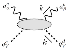
Figure 1: Diagrammatic representation of $\left\langle A_{\alpha}^{a}A_{\beta}^{b}Q_{V}^{c}Q_{V}^{d}\right\rangle$. The other correlation functions can be represented in a similar way.

Before proceeding with the ChPT calculation, we make a final comment on the correlation functions in Eq. (53). Due to the existence of the Pauli-Villars regulator in $D^{\rho\sigma}_{<}(z)$, all the space-time integrals with respect to $x,y,z$ are convergent. Still, if the LECs probe the physics at the scale $q\sim M_{W}$, then the corresponding correlation functions are not fully computed by lattice QCD alone because this will require a lattice spacing of the size $a\sim 1/M_{W}$ which is not achievable in practice. Fortunately, unlike $K_{12}^{r}$ (see the discussion in Sec. II.2), none of the LECs $K_{1}^{r},...,K_{6}^{r}$ is sensitive to physics at the UV-scale, so the use of a typical lattice spacing is sufficient.

IV.3 ChPT representation of the four-point functions

The four-point functions defined in Eq. (52) were already calculated in ChPT to $\mathcal{O}(e^{2}p^{2})$ in Ref. Ananthanarayan:2004qk , but there they worked in the chiral limit and retained only the $g_{\alpha\beta}$ structure, making the results not directly applicable for the lattice. Here, we redo the calculation at the SU(3) symmetric point with non-zero $M_{\phi}$ and include both the $g_{\alpha\beta}$ and $k_{\alpha}k_{\beta}$ structures. Following that reference, we cast our results in terms of the four flavor basis defined below:

$$\hat{e}_{1} = f^{acg}f^{bdg}+f^{adg}f^{bcg}\leavevmode\nobreak\ ,$$

$$\hat{e}_{2} = \delta^{ac}\delta^{bd}+\delta^{ad}\delta^{bc}\leavevmode\nobreak\ ,$$

$$\hat{e}_{3} = d^{acg}d^{bdg}+d^{adg}d^{bcg}\leavevmode\nobreak\ ,$$

$$\hat{e}_{4} = f^{abg}f^{cdg}.$$ (54)

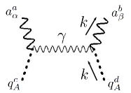
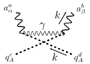
Figure 2: $\mathcal{O}(p^{2})$ contributions to $\left\langle A_{\alpha}^{a}A_{\beta}^{b}Q_{A}^{c}Q_{A}^{d}\right\rangle$.

Up to $\mathcal{O}(e^{2}p^{2})$, the four-point functions read:

$$\left\langle A_{\alpha}^{a}A_{\beta}^{b}Q_{V}^{c}Q_{V}^{d}\right\rangle = iF_{0}^{2}g_{\alpha\beta}\sum_{i=1}^{3}\alpha_{AV}^{(i)}\hat{e}_{i}+iF_{0}^{2}\frac{k_{\alpha}k_{\beta}}{k^{2}-M_{\phi}^{2}}\sum_{i=1}^{4}\beta_{AV}^{(i)}\hat{e}_{i}$$

$$+\left\langle A_{\alpha}^{a}A_{\beta}^{b}Q_{V}^{c}Q_{V}^{d}\right\rangle_{\phi}+\left\langle A_{\alpha}^{a}A_{\beta}^{b}Q_{V}^{c}Q_{V}^{d}\right\rangle_{\gamma}\leavevmode\nobreak\ ,$$

$$\left\langle A_{\alpha}^{a}A_{\beta}^{b}Q_{A}^{c}Q_{A}^{d}\right\rangle = iF_{0}^{2}g_{\alpha\beta}\left[\delta^{ad}\delta^{bc}\frac{F_{0}^{2}}{k^{2}-M_{\gamma}^{2}}-\delta^{ac}\delta^{bd}\frac{F_{0}^{2}}{M_{\gamma}^{2}}\right]+iF_{0}^{2}g_{\alpha\beta}\sum_{i=1}^{3}\alpha_{AA}^{(i)}\hat{e}_{i}$$

$$+iF_{0}^{2}\frac{k_{\alpha}k_{\beta}}{k^{2}-M_{\phi}^{2}}\sum_{i=1}^{4}\beta_{AA}^{(i)}\hat{e}_{i}+\left\langle A_{\alpha}^{a}A_{\beta}^{b}Q_{A}^{c}Q_{A}^{d}\right\rangle_{\phi}+\left\langle A_{\alpha}^{a}A_{\beta}^{b}Q_{A}^{c}Q_{A}^{d}\right\rangle_{\gamma}\leavevmode\nobreak\ ,$$

$$\left\langle V_{\alpha}^{a}V_{\beta}^{b}Q_{V}^{c}Q_{V}^{d}\right\rangle = iF_{0}^{2}g_{\alpha\beta}\alpha_{VV}^{(1)}\hat{e}_{1}+\left\langle V_{\alpha}^{a}V_{\beta}^{b}Q_{V}^{c}Q_{V}^{d}\right\rangle_{\phi}\leavevmode\nobreak\ .$$ (55)

Let us explain the results above. First, the square bracket in $\left\langle A_{\alpha}^{a}A_{\beta}^{b}Q_{A}^{c}Q_{A}^{d}\right\rangle$ represents the only $\mathcal{O}(p^{2})$ contribution that comes from the diagrams shown in Fig. 2 which is, for some reason, missing in Ref. Ananthanarayan:2004qk . All the others are $\mathcal{O}(e^{2}p^{2})$. The coefficients $\alpha^{(i)}$ and $\beta^{(i)}$ contain the contributions from the LECs (as depicted in Fig. 3) as well as the UV-divergent part of the loop contributions . The remaining parts that carry the subscript $\phi$ and $\gamma$ denote the UV-finite contributions of the meson and photon loop diagrams, further detail can be found in Appendix A.

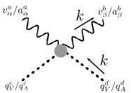
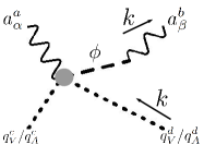
Figure 3: LEC contributions to the correlation functions. The gray dot represents the counterterm vertex.

Let us concentrate on the coefficients $\alpha^{(i)}$ and $\beta^{(i)}$. They read:

$$\alpha_{AV}^{(1)} = 2K_{1}^{r}+2K_{2}^{r}+2K_{5}^{r}+2K_{6}^{r}+4K_{12}^{r}-K_{13}+2K_{14}+\frac{5Z-2}{32\pi^{2}}\ln\frac{\mu^{2}}{M_{\phi}^{2}}\leavevmode\nobreak\ ,$$

$$\alpha_{AV}^{(2)} = -4K_{3}^{r}+2K_{4}^{r}+\frac{4}{3}K_{5}^{r}+\frac{4}{3}K_{6}^{r}+\frac{3Z}{16\pi^{2}}\ln\frac{\mu^{2}}{M_{\phi}^{2}}\leavevmode\nobreak\ ,$$

$$\alpha_{AV}^{(3)} = 6K_{1}^{r}+6K_{2}^{r}+2K_{5}^{r}+2K_{6}^{r}+\frac{9Z}{32\pi^{2}}\ln\frac{\mu^{2}}{M_{\phi}^{2}}\leavevmode\nobreak\ ,$$ (56)

$$\beta_{AV}^{(1)} = -2K_{1}^{r}-2K_{2}^{r}-2K_{5}^{r}-2K_{6}^{r}-2K_{12}^{r}+K_{13}+\frac{5-10Z}{64\pi^{2}}\ln\frac{\mu^{2}}{M_{\phi}^{2}}\leavevmode\nobreak\ ,$$

$$\beta_{AV}^{(2)} = 4K_{3}^{r}-2K_{4}^{r}-\frac{4}{3}K_{5}^{r}-\frac{4}{3}K_{6}^{r}-\frac{3Z}{16\pi^{2}}\ln\frac{\mu^{2}}{M_{\phi}^{2}}\leavevmode\nobreak\ ,$$

$$\beta_{AV}^{(3)} = -6K_{1}^{r}-6K_{2}^{r}-2K_{5}^{r}-2K_{6}^{r}-\frac{9Z}{32\pi^{2}}\ln\frac{\mu^{2}}{M_{\phi}^{2}}\leavevmode\nobreak\ ,$$

$$\beta_{AV}^{(4)} = -2K_{12}^{r}+K_{13}-\frac{1}{64\pi^{2}}\ln\frac{\mu^{2}}{M_{\phi}^{2}}\leavevmode\nobreak\ ,$$ (57)

$$\alpha_{AA}^{(1)} = 2K_{1}^{r}-2K_{2}^{r}+2K_{5}^{r}-2K_{6}^{r}+4K_{12}^{r}+K_{13}+2K_{14}-\frac{5Z+2}{32\pi^{2}}\ln\frac{\mu^{2}}{M_{\phi}^{2}}\leavevmode\nobreak\ ,$$

$$\alpha_{AA}^{(2)} = -4K_{3}^{r}-2K_{4}^{r}+\frac{4}{3}K_{5}^{r}-\frac{4}{3}K_{6}^{r}-\frac{3Z}{16\pi^{2}}\ln\frac{\mu^{2}}{M_{\phi}^{2}}\leavevmode\nobreak\ ,$$

$$\alpha_{AA}^{(3)} = 6K_{1}^{r}-6K_{2}^{r}+2K_{5}^{r}-2K_{6}^{r}-\frac{9Z}{32\pi^{2}}\ln\frac{\mu^{2}}{M_{\phi}^{2}}\leavevmode\nobreak\ ,$$ (58)

$$\beta_{AA}^{(1)} = -2K_{1}^{r}+2K_{2}^{r}-2K_{5}^{r}+2K_{6}^{r}-2K_{12}^{r}-K_{13}+\frac{5+10Z}{64\pi^{2}}\ln\frac{\mu^{2}}{M_{\phi}^{2}}\leavevmode\nobreak\ ,$$

$$\beta_{AA}^{(2)} = 4K_{3}^{r}+2K_{4}^{r}-\frac{4}{3}K_{5}^{r}+\frac{4}{3}K_{6}^{r}+\frac{3Z}{16\pi^{2}}\ln\frac{\mu^{2}}{M_{\phi}^{2}}\leavevmode\nobreak\ ,$$

$$\beta_{AA}^{(3)} = -6K_{1}^{r}+6K_{2}^{r}-2K_{5}^{r}+2K_{6}^{r}+\frac{9Z}{32\pi^{2}}\ln\frac{\mu^{2}}{M_{\phi}^{2}}\leavevmode\nobreak\ ,$$

$$\beta_{AA}^{(4)} = -2K_{12}^{r}-K_{13}-\frac{1}{64\pi^{2}}\ln\frac{\mu^{2}}{M_{\phi}^{2}}\leavevmode\nobreak\ ,$$ (59)

and finally, $\alpha_{VV}^{(1)}=K_{13}+2K_{14}$. They provide an over-complete set of equations to solve for the needed LECs, an example of solutions is given in Appendix B. So in principle one could calculate each correlation function with several flavor combinations to extract the needed coefficients $\alpha^{(i)}$ and $\beta^{(i)}$, and with them one could determine all the $\{K_{i}^{r}\}$ individually. However, if we are only interested in the unsuppressed combination of $\{K_{i}^{r}\}$ that enters $\delta_{\mathrm{em}}^{K^{\pm}l}$ (see Eq. (28)), things are much simpler: It can be obtained from a single four-point function at zero external momentum:

$$\left\langle A_{\alpha}^{1}A_{\beta}^{8}Q_{V}^{8}Q_{V}^{1}\right\rangle_{k=0}=iF_{0}^{2}g_{\alpha\beta}\left[-4K_{3}^{r}+2K_{4}^{r}+\frac{4}{3}K_{5}^{r}+\frac{4}{3}K_{6}^{r}+\frac{3Z}{16\pi^{2}}\left(-1+\ln\frac{\mu^{2}}{M_{\phi}^{2}}\right)\right]\leavevmode\nobreak\ ,$$ (60)

which is the last central result of this paper.

This completes the setup of the problem for the future lattice calculation. The chiral LEC’s are unambiguously related to a 4-point correlation function and the axial $\gamma W$ box. Using lattice QCD simulations, one can expect to determine the LECs with controlled uncertainties and provide useful information for the electromagnetic corrections to $K_{l3}$ decays.

V Conclusions

We have entered a new era where lattice QCD becomes increasingly important in the studies of high-precision electromagnetic effects in low-energy phenomena. In particular, it is now timely to extend its impact to the field of semileptonic beta decays which plays a decisive role in the precision test of the top-row CKM matrix unitarity and the implications for BSM physics therein.

It is expected to be extremely challenging to perform a full lattice QCD calculation to the virtual + real QED corrections to the kaon semileptonic decay rate, of which the estimated time span is of the order of $10^{1}$ years. Given the current status of the CKM unitarity, it is highly desirable to look for an alternative starting point such that lattice QCD can make immediate impact to the field. In this paper we propose a strategy of such kind. We first point out that, at $\mathcal{O}(e^{2}p^{2})$ in chiral power counting, there are only three combinations of LECs that are relevant for $K_{l3}$ and $\pi_{e3}$ decays: $X_{1}$, $\bar{X}_{6}^{\mathrm{phys}}$ and $-2K_{3}^{r}+K_{4}^{r}+(2/3)(K_{5}^{r}+K_{6}^{r})$. Based on a careful comparison between the Sirlin’s representation and the ChPT representation of the QED effects, we show that these LECs can all be pinned down by calculating a few simple quantities on the lattice.

To obtain the LECs $X_{1}$ and $\bar{X}_{6}^{\mathrm{phys}}$, we need to calculate the axial $\gamma W$-box diagrams for the $\pi^{0}\pi^{+}$ and $\pi^{-}K^{0}$ systems in the degenerate limit. The former was already performed in Ref. Feng:2020zdc , which translates into a determination of $(4/3)X_{1}+\bar{X}_{6}^{\mathrm{phys}}$ with 10% accuracy. We observe that the outcome is significantly different from the resonant model calculation widely adopted in the existing $K_{l3}$ RC analysis, which adds to the urgency of our proposed calculations. The $\pi^{-}K^{0}$ axial box can be computed in exactly the same way, and in fact its result will be available in the near future.

On the other hand, the extraction of the LECs $\{K_{i}^{r}\}$ will be based on the lattice calculation of the four-point correlation functions defined in Eq.(53) which can be done using, e.g., sequential-source propagators. In particular, we show an example in Appendix B where all individual $\{K_{i}^{r}\}$ are obtained from the coefficients $\{\beta^{(i)}\}$ in the four-point functions. In practice it is of course not so trivial, because these coefficients are associated to the $k_{\alpha}k_{\beta}$ structure that is sensitive to the direction of the external momentum $k$, which may lead to extra systematic uncertainties due to the breaking of the exact rotational symmetry on the lattice (it is not possible to solve for all individual $\{K_{i}^{r}\}$ using only the simpler coefficients $\{\alpha^{(i)}\}$ without imposing further assumptions, such as large-$N_{c}$ approximation, which one normally avoids in first-principles calculations). Fortunately, as far as the relevant linear combination $-2K_{3}^{r}+K_{4}^{r}+(2/3)(K_{5}^{r}+K_{6}^{r})$ is concerned, one needs only to calculate a single four-point correlation function with zero external momentum, as indicated in Eq.(60). We will defer the discussions of the actual lattice QCD setup needed for such a calculation to a future work.

Our proposed calculation will not only improve the precision of the $|V_{us}|$ extraction from $K_{l3}$ alone, but will also reduce the theoretical uncertainty in the ratio $R_{V}=\Gamma_{K_{l3}}/\Gamma_{\pi_{e3}}$ that helps us to better understand the disagreement between the $K_{l2}$ and $K_{l3}$ extractions of $|V_{us}|$.

Appendix A loop contributions to the four-point functions

In this Appendix we present the UV-finite parts of the one-loop contributions to the four-point correlation functions in Eq. (55).

A.1 $\mathcal{O}(e^{2}p^{2})$ contributions from meson loops

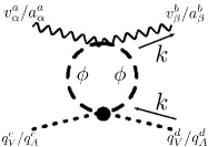
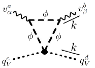
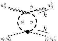
Figure 4: Contributions from meson loops. The black circle denotes the $\mathcal{O}(e^{2})$ vertex. The third diagram contains a meson pole.

The meson loop contributions are depicted in Fig. 4. The results are:

$$\left\langle A_{\alpha}^{a}A_{\beta}^{b}Q_{V}^{c}Q_{V}^{d}\right\rangle_{\phi} = -\left\langle A_{\alpha}^{a}A_{\beta}^{b}Q_{A}^{c}Q_{A}^{d}\right\rangle_{\phi}$$

$$= iF_{0}^{2}\frac{Z}{16\pi^{2}}\left(\frac{5}{2}\hat{e}_{1}+3\hat{e}_{2}+\frac{9}{2}\hat{e}_{3}\right)\left(1+\Lambda(k^{2},M_{\phi})\right)\left(g_{\alpha\beta}-\frac{k_{\alpha}k_{\beta}}{k^{2}-M_{\phi}^{2}}\right)$$

$$\left\langle V_{\alpha}^{a}V_{\beta}^{b}Q_{V}^{c}Q_{V}^{d}\right\rangle_{\phi} = 0,$$ (61)

where

$$\Lambda(k^{2},M_{\phi})=\frac{\sqrt{k^{2}(k^{2}-4M_{\phi}^{2})}}{k^{2}}\ln\left(\frac{\sqrt{k^{2}(k^{2}-4M_{\phi}^{2})}-k^{2}+2M_{\phi}^{2}}{2M_{\phi}^{2}}\right).$$ (62)

A.2 $\mathcal{O}(e^{2}p^{2})$ contributions from photon loops

The photon loop contributions involve more Feynman diagrams, so for the benefits of future cross-check, we split them into two pieces: $\left\langle...\right\rangle_{\gamma}=\left\langle...\right\rangle_{\gamma_{1}}+\left\langle...\right\rangle_{\gamma_{2}}$, where the two terms on the RHS denote contribution without and with a meson pole, respectively.

A.2.1 without meson pole

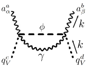
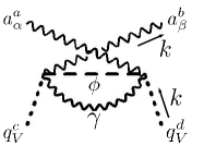
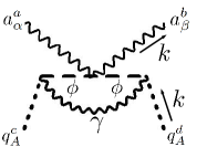
Figure 5: Contributions from photon loops without a meson pole.

The photon loop contributions without a meson pole are depicted in Fig. 5. The results read:

$$\left\langle A_{\alpha}^{a}A_{\beta}^{b}Q_{V}^{c}Q_{V}^{d}\right\rangle_{\gamma_{1}} = -iF_{0}^{2}\frac{1}{16\pi^{2}}\frac{\hat{e}_{1}-\hat{e}_{4}}{2}\left(\frac{k^{2}-M_{\phi}^{2}}{k^{2}}\ln\frac{M_{\phi}^{2}}{M_{\phi}^{2}-k^{2}}+1\right)g_{\alpha\beta}$$

$$\left\langle A_{\alpha}^{a}A_{\beta}^{b}Q_{A}^{c}Q_{A}^{d}\right\rangle_{\gamma_{1}} = -iF_{0}^{2}\frac{1}{16\pi^{2}}\hat{e}_{1}\left(\frac{2M_{\phi}^{2}-k^{2}}{2M_{\phi}^{2}}\Lambda(k^{2},M_{\phi})+\frac{(k^{2}-M_{\phi}^{2})^{2}}{2k^{2}M_{\phi}^{2}}\ln\frac{M_{\phi}^{2}}{M_{\phi}^{2}-k^{2}}+\frac{1}{2}\right)g_{\alpha\beta}.$$

A.2.2 with meson pole

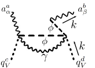
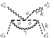
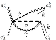
Figure 6: Contributions from photon loops with a meson pole.

The contributions from photon loops with a meson pole are depicted in Fig. 6. The results read:

$$\left\langle A_{\alpha}^{a}A_{\beta}^{b}Q_{V}^{c}Q_{V}^{d}\right\rangle_{\gamma_{2}} = iF_{0}^{2}\frac{1}{16\pi^{2}}\frac{\hat{e}_{1}-\hat{e}_{4}}{2}\frac{3k^{2}+M_{\phi}^{2}}{2k^{2}}\left(\frac{k^{2}-M_{\phi}^{2}}{k^{2}}\ln\frac{M_{\phi}^{2}}{M_{\phi}^{2}-k^{2}}+1\right)\frac{k_{\alpha}k_{\beta}}{k^{2}-M_{\phi}^{2}}$$

$$\left\langle A_{\alpha}^{a}A_{\beta}^{b}Q_{A}^{c}Q_{A}^{d}\right\rangle_{\gamma_{2}} = iF_{0}^{2}\frac{1}{16\pi^{2}}\left\{\hat{e}_{1}\left[\frac{2M_{\phi}^{2}-k^{2}}{2M_{\phi}^{2}}\Lambda(k^{2},M_{\phi})+\frac{2(k^{2})^{3}-3(k^{2})^{2}M_{\phi}^{2}+2k^{2}M_{\phi}^{4}-M_{\phi}^{6}}{4(k^{2})^{2}M_{\phi}^{2}}\right.\right.$$ (64)

$$\left.\times\ln\frac{M_{\phi}^{2}}{M_{\phi}^{2}-k^{2}}+\frac{3k^{2}+M_{\phi}^{2}}{4k^{2}}\right]+\hat{e}_{4}\left[-\frac{(k^{2})^{2}+4k^{2}M_{\phi}^{2}-5M_{\phi}^{4}}{4(k^{2})^{2}}\ln\frac{M_{\phi}^{2}}{M_{\phi}^{2}-k^{2}}\right.$$

$$\left.\left.-\frac{k^{2}+5M_{\phi}^{2}}{4k^{2}}\right]\right\}\frac{k_{\alpha}k_{\beta}}{k^{2}-M_{b}^{2}}.$$

Appendix B Obtaining every $K_{i}^{r}$ individually

In this Appendix we present one (out of the many possible) set of solutions for $K_{1}^{r},...,K_{6}^{r}$ in terms of the coefficients $\{\alpha^{(i)},\beta^{(i)}\}$ defined in Eq. (55). Here we make use of only $\{\beta^{(i)}\}$:

$$K_{1}^{r} = \frac{1}{8}\left(\beta_{AA}^{(1)}-\beta_{AA}^{(3)}-\beta_{AA}^{(4)}+\beta_{AV}^{(1)}-\beta_{AV}^{(3)}-\beta_{AV}^{(4)}-\frac{3}{16\pi^{2}}\ln\frac{\mu^{2}}{M_{\phi}^{2}}\right)$$

$$K_{2}^{r} = \frac{1}{8}\left(-\beta_{AA}^{(1)}+\beta_{AA}^{(3)}+\beta_{AA}^{(4)}+\beta_{AV}^{(1)}-\beta_{AV}^{(3)}-\beta_{AV}^{(4)}-\frac{Z}{4\pi^{2}}\ln\frac{\mu^{2}}{M_{\phi}^{2}}\right)$$

$$K_{3}^{r} = \frac{1}{24}\left(-3\beta_{AA}^{(1)}+3\beta_{AA}^{(2)}+\beta_{AA}^{(3)}+3\beta_{AA}^{(4)}-3\beta_{AV}^{(1)}+3\beta_{AV}^{(2)}+\beta_{AV}^{(3)}+3\beta_{AV}^{(4)}+\frac{9}{16\pi^{2}}\ln\frac{\mu^{2}}{M_{\phi}^{2}}\right)$$

$$K_{4}^{r} = \frac{1}{12}\left(-3\beta_{AA}^{(1)}+3\beta_{AA}^{(2)}+\beta_{AA}^{(3)}+3\beta_{AA}^{(4)}+3\beta_{AV}^{(1)}-3\beta_{AV}^{(2)}-\beta_{AV}^{(3)}-3\beta_{AV}^{(4)}-\frac{3Z}{4\pi^{2}}\ln\frac{\mu^{2}}{M_{\phi}^{2}}\right)$$

$$K_{5}^{r} = \frac{1}{8}\left(-3\beta_{AA}^{(1)}+\beta_{AA}^{(3)}+3\beta_{AA}^{(4)}-3\beta_{AV}^{(1)}+\beta_{AV}^{(3)}+3\beta_{AV}^{(4)}+\frac{9}{16\pi^{2}}\ln\frac{\mu^{2}}{M_{\phi}^{2}}\right)$$

$$K_{6}^{r} = \frac{1}{8}\left(3\beta_{AA}^{(1)}-\beta_{AA}^{(3)}-3\beta_{AA}^{(4)}-3\beta_{AV}^{(1)}+\beta_{AV}^{(3)}+3\beta_{AV}^{(4)}-\frac{3Z}{8\pi^{2}}\ln\frac{\mu^{2}}{M_{\phi}^{2}}\right).$$ (65)

References

- (1) C.-Y. Seng, M. Gorchtein, H. H. Patel and M. J. Ramsey-Musolf, Reduced Hadronic Uncertainty in the Determination of , Phys. Rev. Lett. 121 (2018), no. 24 241804 [1807.10197].
- (2) C. Y. Seng, M. Gorchtein and M. J. Ramsey-Musolf, Dispersive evaluation of the inner radiative correction in neutron and nuclear decay, Phys. Rev. D100 (2019), no. 1 013001 [1812.03352].
- (3) Particle Data Group Collaboration, P. Zyla et. al., Review of Particle Physics, PTEP 2020 (2020), no. 8 083C01.
- (4) Particle Data Group Collaboration, M. Tanabashi et. al., Review of Particle Physics, Phys. Rev. D98 (2018), no. 3 030001.
- (5) M. Gonzalez-Alonso, O. Naviliat-Cuncic and N. Severijns, New physics searches in nuclear and neutron decay, Prog. Part. Nucl. Phys. 104 (2019) 165–223 [1803.08732].
- (6) D. Bryman and R. Shrock, Improved Constraints on Sterile Neutrinos in the MeV to GeV Mass Range, Phys. Rev. D 100 (2019), no. 5 053006 [1904.06787].
- (7) B. Belfatto, R. Beradze and Z. Berezhiani, The CKM unitarity problem: A trace of new physics at the TeV scale?, Eur. Phys. J. C 80 (2020), no. 2 149 [1906.02714].
- (8) V. Cirigliano, A. Garcia, D. Gazit, O. Naviliat-Cuncic, G. Savard and A. Young, Precision Beta Decay as a Probe of New Physics, 1907.02164.
- (9) W. Tan, Laboratory tests of the ordinary-mirror particle oscillations and the extended CKM matrix, 1906.10262.
- (10) D. Bryman and R. Shrock, Constraints on Sterile Neutrinos in the MeV to GeV Mass Range, Phys. Rev. D 100 (2019) 073011 [1909.11198].
- (11) Y. Grossman, E. Passemar and S. Schacht, On the Statistical Treatment of the Cabibbo Angle Anomaly, JHEP 07 (2020) 068 [1911.07821].
- (12) A. M. Coutinho, A. Crivellin and C. A. Manzari, Global Fit to Modified Neutrino Couplings and the Cabibbo-Angle Anomaly, Phys. Rev. Lett. 125 (2020), no. 7 071802 [1912.08823].
- (13) K. Cheung, W.-Y. Keung, C.-T. Lu and P.-Y. Tseng, Vector-like Quark Interpretation for the CKM Unitarity Violation, Excess in Higgs Signal Strength, and Bottom Quark Forward-Backward Asymmetry, JHEP 05 (2020) 117 [2001.02853].
- (14) A. Crivellin and M. Hoferichter, Beta decays as sensitive probes of lepton flavor universality, 2002.07184.
- (15) M. Endo and S. Mishima, Muon g-2 and CKM unitarity in extra lepton models, JHEP 08 (2020), no. 08 004 [2005.03933].
- (16) B. Capdevila, A. Crivellin, C. A. Manzari and M. Montull, Explaining and the Cabibbo Angle Anomaly with a Vector Triplet, 2005.13542.
- (17) M. Kirk, The Cabibbo anomaly versus electroweak precision tests – an exploration of extensions of the Standard Model, 2008.03261.
- (18) N. Carrasco, V. Lubicz, G. Martinelli, C. Sachrajda, N. Tantalo, C. Tarantino and M. Testa, QED Corrections to Hadronic Processes in Lattice QCD, Phys. Rev. D 91 (2015), no. 7 074506 [1502.00257].
- (19) V. Lubicz, G. Martinelli, C. Sachrajda, F. Sanfilippo, S. Simula and N. Tantalo, Finite-Volume QED Corrections to Decay Amplitudes in Lattice QCD, Phys. Rev. D 95 (2017), no. 3 034504 [1611.08497].
- (20) D. Giusti, V. Lubicz, G. Martinelli, C. T. Sachrajda, F. Sanfilippo, S. Simula, N. Tantalo and C. Tarantino, First lattice calculation of the QED corrections to leptonic decay rates, Phys. Rev. Lett. 120 (2018), no. 7 072001 [1711.06537].
- (21) M. Di Carlo, D. Giusti, V. Lubicz, G. Martinelli, C. T. Sachrajda, F. Sanfilippo, S. Simula and N. Tantalo, Light-meson leptonic decay rates in lattice QCD+QED, Phys. Rev. D100 (2019), no. 3 034514 [1904.08731].
- (22) D. Giusti, V. Lubicz, G. Martinelli, C. Sachrajda, F. Sanfilippo, S. Simula and N. Tantalo, Radiative corrections to decay amplitudes in lattice QCD, PoS LATTICE2018 (2019) 266 [1811.06364].
- (23) C. Sachrajda, M. Di Carlo, G. Martinelli, D. Giusti, V. Lubicz, F. Sanfilippo, S. Simula and N. Tantalo, Radiative corrections to semileptonic decay rates, in 37th International Symposium on Lattice Field Theory, 10, 2019. 1910.07342.
- (24) USQCD Collaboration, V. Cirigliano, Z. Davoudi, T. Bhattacharya, T. Izubuchi, P. E. Shanahan, S. Syritsyn and M. L. Wagman, The Role of Lattice QCD in Searches for Violations of Fundamental Symmetries and Signals for New Physics, Eur. Phys. J. A 55 (2019), no. 11 197 [1904.09704].
- (25) X. Feng, M. Gorchtein, L.-C. Jin, P.-X. Ma and C.-Y. Seng, First-principles calculation of electroweak box diagrams from lattice QCD, Phys. Rev. Lett. 124 (2020), no. 19 192002 [2003.09798].
- (26) C.-Y. Seng, X. Feng, M. Gorchtein and L.-C. Jin, Joint lattice QCD–dispersion theory analysis confirms the quark-mixing top-row unitarity deficit, Phys. Rev. D 101 (2020), no. 11 111301 [2003.11264].
- (27) V. Cirigliano, M. Knecht, H. Neufeld, H. Rupertsberger and P. Talavera, Radiative corrections to K(l3) decays, Eur. Phys. J. C23 (2002) 121–133 [hep-ph/0110153].
- (28) V. Cirigliano, M. Giannotti and H. Neufeld, Electromagnetic effects in K(l3) decays, JHEP 11 (2008) 006 [0807.4507].
- (29) B. Ananthanarayan and B. Moussallam, Four-point correlator constraints on electromagnetic chiral parameters and resonance effective Lagrangians, JHEP 06 (2004) 047 [hep-ph/0405206].
- (30) S. Descotes-Genon and B. Moussallam, Radiative corrections in weak semi-leptonic processes at low energy: A Two-step matching determination, Eur. Phys. J. C42 (2005) 403–417 [hep-ph/0505077].
- (31) W. J. Marciano, Precise determination of —V(us)— from lattice calculations of pseudoscalar decay constants, Phys. Rev. Lett. 93 (2004) 231803 [hep-ph/0402299].
- (32) A. Czarnecki, W. J. Marciano and A. Sirlin, Pion beta decay and Cabibbo-Kobayashi-Maskawa unitarity, Phys. Rev. D 101 (2020), no. 9 091301 [1911.04685].
- (33) T. Kinoshita and A. Sirlin, Radiative corrections to Fermi interactions, Phys. Rev. 113 (1959) 1652–1660.
- (34) A. Sirlin, General Properties of the Electromagnetic Corrections to the Beta Decay of a Physical Nucleon, Phys. Rev. 164 (1967) 1767–1775.
- (35) A. Sirlin, Radiative corrections to g(v)/g(mu) in simple extensions of the su(2) x u(1) gauge model, Nucl. Phys. B 71 (1974) 29–51.
- (36) A. Sirlin, Current Algebra Formulation of Radiative Corrections in Gauge Theories and the Universality of the Weak Interactions, Rev. Mod. Phys. 50 (1978) 573. [Erratum: Rev. Mod. Phys.50,905(1978)].
- (37) A. Sirlin, Radiative Corrections in the SU(2)-L x U(1) Theory: A Simple Renormalization Framework, Phys. Rev. D 22 (1980) 971–981.
- (38) C.-Y. Seng, D. Galviz and U.-G. Meißner, A New Theory Framework for the Electroweak Radiative Corrections in Decays, JHEP 02 (2020) 069 [1910.13208].
- (39) J. Erler, Electroweak radiative corrections to semileptonic tau decays, Rev. Mex. Fis. 50 (2004) 200–202 [hep-ph/0211345].
- (40) L. S. Brown, Perturbation theory and selfmass insertions, Phys. Rev. 187 (1969) 2260–2265.
- (41) J. Gasser and H. Leutwyler, Chiral Perturbation Theory: Expansions in the Mass of the Strange Quark, Nucl. Phys. B250 (1985) 465–516.
- (42) R. Urech, Virtual photons in chiral perturbation theory, Nucl. Phys. B433 (1995) 234–254 [hep-ph/9405341].
- (43) H. Neufeld and H. Rupertsberger, The Electromagnetic interaction in chiral perturbation theory, Z. Phys. C 71 (1996) 131–138 [hep-ph/9506448].
- (44) M. Knecht, H. Neufeld, H. Rupertsberger and P. Talavera, Chiral perturbation theory with virtual photons and leptons, Eur. Phys. J. C12 (2000) 469–478 [hep-ph/9909284].
- (45) V. Cirigliano, M. Knecht, H. Neufeld and H. Pichl, The Pionic beta decay in chiral perturbation theory, Eur. Phys. J. C 27 (2003) 255–262 [hep-ph/0209226].
- (46) V. Cirigliano, K(e3) and pi(e3) decays: Radiative corrections and CKM unitarity, in 38th Rencontres de Moriond on Electroweak Interactions and Unified Theories, 5, 2003. hep-ph/0305154.
- (47) W. J. Marciano and A. Sirlin, Radiative corrections to pi(lepton 2) decays, Phys. Rev. Lett. 71 (1993) 3629–3632.
- (48) V. Cirigliano, G. Ecker, H. Neufeld, A. Pich and J. Portoles, Kaon Decays in the Standard Model, Rev. Mod. Phys. 84 (2012) 399 [1107.6001].
- (49) N. Meister and D. Yennie, Radiative Corrections to High-Energy Scattering Processes, Phys. Rev. 130 (1963) 1210–1229.
- (50) C.-Y. Seng and U.-G. Meißner, Toward a First-Principles Calculation of Electroweak Box Diagrams, Phys. Rev. Lett. 122 (2019), no. 21 211802 [1903.07969].
- (51) C. Bouchard, C. C. Chang, T. Kurth, K. Orginos and A. Walker-Loud, On the Feynman-Hellmann Theorem in Quantum Field Theory and the Calculation of Matrix Elements, Phys. Rev. D 96 (2017), no. 1 014504 [1612.06963].
- (52) A. Chambers, R. Horsley, Y. Nakamura, H. Perlt, P. Rakow, G. Schierholz, A. Schiller, K. Somfleth, R. Young and J. Zanotti, Nucleon Structure Functions from Operator Product Expansion on the Lattice, Phys. Rev. Lett. 118 (2017), no. 24 242001 [1703.01153].
- (53) M. Passera, K. Philippides and A. Sirlin, Observations on the radiative corrections to pion -decay, Phys. Rev. D 84 (2011) 094030 [1109.1069].
- (54) W. Beenakker and A. Denner, Infrared Divergent Scalar Box Integrals With Applications in the Electroweak Standard Model, Nucl. Phys. B 338 (1990) 349–370.
- (55) J. Bijnens and J. Prades, Electromagnetic corrections for pions and kaons: Masses and polarizabilities, Nucl. Phys. B490 (1997) 239–271 [hep-ph/9610360].
- (56) B. Moussallam, A Sum rule approach to the violation of Dashen’s theorem, Nucl. Phys. B 504 (1997) 381–414 [hep-ph/9701400].
- (57) H. H. Patel, Package-X: A Mathematica package for the analytic calculation of one-loop integrals, Comput. Phys. Commun. 197 (2015) 276–290 [1503.01469].
- (58) H. H. Patel, Package-X 2.0: A Mathematica package for the analytic calculation of one-loop integrals, Comput. Phys. Commun. 218 (2017) 66–70 [1612.00009].