h Cavendish-HEP-20/11, VBSCAN-PUB-09-20
NLO QCD and EW corrections to vector-boson scattering into ZZ at the LHC

Abstract

We present the first calculation of the full next-to-leading-order electroweak and QCD corrections for vector-boson scattering (VBS) into a pair of Z bosons at the LHC. We consider specifically the process $\text{p}\text{p}\to\text{e}^{+}\text{e}^{-}\mu^{+}\mu^{-}\text{j}\text{j}+X$ at orders $\mathcal{O}{\left(\alpha^{7}\right)}$ and $\mathcal{O}{\left(\alpha_{s}\alpha^{6}\right)}$ and take all off-shell and interference contributions into account. Owing to the presence of enhanced Sudakov logarithms, the electroweak corrections amount to $-16\%$ of the leading-order electroweak fiducial cross section and induce significant shape distortions of differential distributions. The QCD corrections on the other hand are larger ($+24\%$) than typical QCD corrections in VBS. This originates from considering the full computation including tri-boson contributions in a rather inclusive phase space. We also provide a leading-order analysis of all contributions to the cross section for $\text{p}\text{p}\to\text{e}^{+}\text{e}^{-}\mu^{+}\mu^{-}\text{j}\text{j}+X$ in a realistic setup.

1 Introduction

The non-observation of physics not described by the Standard Model (SM) at the Large Hadron Collider (LHC) shifts into the focus of interest tests of the SM of particle physics and in particular of the mechanism of electroweak (EW) symmetry breaking. A particularly important class of processes in this respect is vector-boson scattering (VBS). It is not only sensitive to the scalar sector of the EW theory but also to non-standard triple and quartic gauge-boson couplings.

The scattering of like-sign W bosons as well as WZ has been observed Aad:2014zda ; Khachatryan:2014sta ; Aaboud:2016ffv ; Sirunyan:2017ret ; Aaboud:2018ddq ; Sirunyan:2019ksz ; Aaboud:2019nmv ; Sirunyan:2020gyx by both ATLAS and CMS in leptonic final states. Quite recently, measurements of VBS into a pair of leptonically decaying Z bosons, which allows for a cleaner experimental detection albeit with lower hadronic cross section, have been published by both experiments Sirunyan:2017fvv ; Aad:2020zbq ; CMS:2020zly . Moreover, EW di-boson production in association with a high-mass di-jet system in semileptonic final states has been searched for Sirunyan:2019der ; Aad:2019xxo .

Theoretically, VBS has been studied since a long time. NLO QCD corrections to all VBS processes exist for more than ten years (see Refs. Baglio:2014uba ; Rauch:2016pai and references therein). On the other hand, EW corrections to these processes have become available only recently Biedermann:2016yds ; Biedermann:2017bss ; Denner:2019tmn . Thereby it has been found that EW corrections to fiducial cross sections of VBS are generically at the level of $-15\%$ Biedermann:2016yds . This has been confirmed by complete calculations for the scattering of $\text{W}^{+}\text{W}^{+}$ Biedermann:2017bss and WZ pairs Denner:2019tmn . Furthermore, for like-sign W scattering an event generator including EW and QCD corrections is available Chiesa:2019ulk .

In this article, we present for the first time NLO EW corrections to VBS into a pair of Z bosons at the LHC, considering specifically the fully leptonic final state $\text{e}^{+}\text{e}^{-}\mu^{+}\mu^{-}\text{j}\text{j}$. The prospects of this channel for the high-luminosity and high-energy upgrade of the LHC have been studied in Ref. CMS:2018mbt . NLO QCD corrections to the purely EW VBS process in the so-called VBS approximation, which neglects $s$-channel diagrams and interferences between $u$-channel and $t$-channel diagrams, have been presented in Ref. Jager:2006cp . These corrections have been matched Jager:2013iza to a QCD parton shower via the POWHEG BOX framework Alioli:2010xd . NLO QCD corrections to the corresponding QCD-induced process have been provided in Ref. Campanario:2014ioa . Very recently, loop-induced ZZ production with up to 2 jets merged and matched to parton showers has been studied Li:2020nmi .

The leading-order (LO) cross section for $\text{p}\text{p}\to\text{e}^{+}\text{e}^{-}\mu^{+}\mu^{-}\text{j}\text{j}+X$ receives contributions of orders $\mathcal{O}{\left(\alpha^{6}\right)}$ (EW contributions), $\mathcal{O}{\left(\alpha_{s}\alpha^{5}\right)}$ (interference), and $\mathcal{O}{\left(\alpha_{s}^{2}\alpha^{4}\right)}$ (QCD-induced contributions). The VBS subprocess is part of the gauge-invariant EW contributions. In the experimental analysis, the three contributions are often referred to as signal, interference, and QCD background, respectively. While the QCD-induced contributions are larger than the EW ones for typical VBS cuts, the interference is smaller than the latter. Since gluon-induced contributions at the order $\mathcal{O}{\left(\alpha_{s}^{4}\alpha^{4}\right)}$ contribute sizeably, we include them in our analysis. In this paper we focus on the NLO EW and QCD corrections to the LO EW contributions. More precisely, we consider the complete gauge-invariant set of contributions at orders $\mathcal{O}{\left(\alpha^{7}\right)}$ and $\mathcal{O}{\left(\alpha_{s}\alpha^{6}\right)}$. While the former are pure EW corrections to the LO EW contributions, the latter receive contributions from the QCD corrections to the LO EW contributions as well as from EW corrections to the LO interferences. In our NLO calculation we do not rely on approximations but take into account the full set of diagrams relevant at the corresponding perturbative order including all interference contributions. We also compare the full NLO EW corrections with the ones obtained within a Sudakov approximation.

The final state $\text{e}^{+}\text{e}^{-}\mu^{+}\mu^{-}\text{j}\text{j}$ leads to a wide-spread variety of contributing partonic channels. This renders the full calculation at NLO EW and especially at NLO QCD technically very demanding and CPU-time intensive.

This article is structured as follows: In Section 2 the considered process and the different contributions are described. In addition, details of our calculation including the checks to validate our results are presented. Section 3 contains numerical results and their description. Lastly, in Section 4 a summary and concluding remarks are given.

2 Description of the calculation

2.1 Leading-order contributions

We are studying the process

$$\text{p}\text{p}\rightarrow{\text{e}^{+}\text{e}^{-}\mu^{+}\mu^{-}\text{j}\text{j}}+X.$$ (1)

At LO, VBS appears in quark-induced partonic channels $\mathrm{qq}\rightarrow\mathrm{e^{+}e^{-}\mu^{+}\mu^{-}qq}$ (q generically stands for a quark or anti-quark). The amplitudes for these processes receive contributions of order $\mathcal{O}{\left(g^{6}\right)}$ as well as of order $\mathcal{O}{\left(g_{\mathrm{s}}^{2}g^{4}\right)}$, where $g$ and $g_{\mathrm{s}}$ denote the EW and strong coupling constant, respectively.

We neglect quark mixing and use a unit quark-mixing matrix. Since a non-trivial quark-mixing matrix would only affect the $s$-channel contributions and the NLO corrections, its effects are suppressed.

Some sample diagrams of order $\mathcal{O}{\left(g^{6}\right)}$ are shown in Figures 1(a)–1(h).

(a)

(b)

(c)

(d)

(e)

(f)

(g)

(h)

(i)

Figure 1: Examples of tree-level Feynman diagrams.

The diagrams in Figures 1(a) and 1(b) represent the characteristic $t$-channel VBS topology. While the first diagram illustrates the scattering of $\text{W}^{+}\text{W}^{-}$ into ZZ, the second one exemplifies ZZ scattering, which takes place only via Higgs exchange. Higgs-exchange $s$-channel diagrams arise in VBS into ZZ as a new feature with respect to same-sign W and WZ scattering. However, partonic channels involving only ZZ scattering are suppressed with respect to those involving the subprocess $\text{W}^{+}\text{W}^{-}\to\text{Z}\text{Z}$. Doubly-resonant, singly-resonant, and non-resonant diagrams of non-VBS type contribute to the partonic processes at order $\mathcal{O}{\left(g^{6}\right)}$, as illustrated in Figures 1(c), 1(d), and 1(e), respectively. Besides $t$- and $u$-channel diagrams also $s$-channel diagrams show up for some partonic processes (Figure 1(f)). In particular, $s$-channel diagrams corresponding to triple gauge-boson production, both for WZZ and ZZZ production appear as depicted in Figures 1(g) and 1(h). Lastly, diagrams at the order $\mathcal{O}{\left(g^{4}g_{s}^{2}\right)}$ are characterised by $t$-channel gluon exchange between the two quark lines (see Figure 1(i)). While in the diagrams we specify only Z bosons in $s$-channel propagators to stress the contributions to the intermediate ZZ state, corresponding diagrams with photons are also included in our computation. In fact, we take into account the complete set of diagrams for the given six-fermion final state.

Consequently, at the level of squared amplitudes three kinds of gauge-invariant contributions exist, purely EW contributions at $\mathcal{O}{\left(\alpha^{6}\right)}$, QCD-induced contributions at order $\mathcal{O}{\left(\alpha_{\text{s}}^{2}\alpha^{4}\right)}$ and contributions at order $\mathcal{O}{\left(\alpha_{\text{s}}\alpha^{5}\right)}$, which result from the interference of diagrams at order $\mathcal{O}{\left(g^{6}\right)}$ and $\mathcal{O}{\left(g_{\mathrm{s}}^{2}g^{4}\right)}$. Owing to the colour structure, the latter contributions are only non-vanishing, if diagrams of two different kinematic channels ($s$, $t$, $u$) with all 4 external quarks in the same generation are interfered, such as the diagrams in Figure 1(f) and Figure 1(i).

We do not consider contributions with bottom quarks in the initial state, which are PDF suppressed, and also do not include final states with bottom quarks. Then 60 partonic quark-induced channels contribute compared to 40 for WZ and 12 for $\text{W}^{\pm}\text{W}^{\pm}$ scattering (not counting $\text{q}\text{q}^{\prime}$ and $\text{q}^{\prime}\text{q}$ initial states separately). Out of these 60 channels, 24 receive non-vanishing interference contributions between different coupling orders that make up the contribution of order $\mathcal{O}{\left(\alpha_{\text{s}}\alpha^{5}\right)}$. At order $\mathcal{O}{\left(\alpha_{\text{s}}^{2}\alpha^{4}\right)}$, in addition to the 60 quark-induced channels, channels with one or two gluons in the initial state contribute. Given the large gluon luminosity at the LHC, the latter are one of the reasons for the enhancement of the QCD-induced contributions over the EW ones.

Further contributions at orders $\mathcal{O}{\left(\alpha^{6}\right)}$ and $\mathcal{O}{\left(\alpha_{\text{s}}\alpha^{5}\right)}$ result from photon-induced processes with $\gamma\gamma$, $\gamma\text{g}$ and $\gamma\text{q}$ initial states. Such contributions were found to be below $0.5\%$ for WZ scattering Denner:2019tmn , which is also expected for VBS into ZZ. These contributions are neglected in this work.

In contrast to final states corresponding to charged $\text{W}^{\pm}\text{W}^{\pm}$ and WZ scattering, the $\text{e}^{+}\text{e}^{-}\mu^{+}\mu^{-}\text{j}\text{j}$ final state receives contributions from the loop-induced partonic process $\text{g}\text{g}\to\text{e}^{+}\text{e}^{-}\mu^{+}\mu^{-}\text{g}\text{g}$ at order $\mathcal{O}{\left(\alpha_{\text{s}}^{4}\alpha^{4}\right)}$ (see Figure 2 for sample diagrams). We include these contributions in our leading-order analysis.

(a)

(b)

Figure 2: Sample diagrams for the loop-induced process $\text{g}\text{g}\to\text{e}^{+}\text{e}^{-}\mu^{+}\mu^{-}\text{g}\text{g}$.

2.2 Virtual corrections

We compute NLO corrections of orders $\mathcal{O}{\left(\alpha^{7}\right)}$ and $\mathcal{O}{\left(\alpha_{\text{s}}\alpha^{6}\right)}$ to the process (1).

(a)

(b)

(c)

(d)

(e)

(f)

Figure 3: Sample one-loop diagrams.

Virtual corrections of order $\mathcal{O}{\left(\alpha^{7}\right)}$ result from interfering purely EW loop diagrams of order $\mathcal{O}{\left(g^{8}\right)}$ with tree diagrams of order $\mathcal{O}{\left(g^{6}\right)}$ and are thus EW corrections to the LO EW diagrams. Examples for loop diagrams of order $\mathcal{O}{\left(g^{8}\right)}$ are depicted Figures 3(a)–3(b). While corrections to VBS involve diagrams with up to 6-point functions (Figure 3(a)), non-resonant diagrams contain up to 8-point functions (Figure 3(b)).

Virtual corrections of order $\mathcal{O}{\left(\alpha_{\text{s}}\alpha^{6}\right)}$ have different sources. First, loop diagrams of order $\mathcal{O}{\left(g^{6}g_{\mathrm{s}}^{2}\right)}$ interfere with tree diagrams of order $\mathcal{O}{\left(g^{6}\right)}$. Such loop diagrams (see Figures 3(c)–3(f) for examples) can be viewed as QCD corrections to diagrams of order $\mathcal{O}{\left(g^{6}\right)}$. However, the diagrams in Figures 3(e)–3(f) can also be viewed as EW corrections to diagrams of order $\mathcal{O}{\left(g^{4}g_{\mathrm{s}}^{2}\right)}$. As a consequence EW and QCD-induced contributions cannot be separated at order $\mathcal{O}{\left(\alpha_{\text{s}}\alpha^{6}\right)}$ on the basis of Feynman diagrams. While diagrams with gluons attached to a single quark line (see Figure 3(c)) contribute for all partonic channels, diagrams with gluon exchange between different quark lines only contribute for partonic processes that receive contributions of different kinematic channels such as those in Figures 3(e) and 3(f), which interfere with the LO diagram Figure 1(a). In the VBS approximation only $t$- and $u$-channel diagrams are taken into account and no interferences between different kinematic channels. Then all corrections of $\mathcal{O}{\left(\alpha_{\text{s}}\alpha^{6}\right)}$ can be interpreted as QCD corrections to the EW LO diagrams.

We do not include contributions of partonic channels with external bottom quarks or photons in the initial state in the virtual corrections.

2.3 Real corrections

In addition to the virtual corrections also real photon and gluon emission needs to be considered. Some related Feynman diagrams are shown in Figure 4.

(a)

(b)

(c)

(d)

(e)

(f)

Figure 4: Sample diagrams for real corrections.

In the quark-induced channels, emission of a real photon from a quark, a W boson, or a charged lepton gives rise to the partonic processes $\text{q}\text{q}\rightarrow{\text{e}^{+}\text{e}^{-}\mu^{+}\mu^{-}\text{q}\text{q}\gamma}$. These furnish the real EW corrections to the LO EW diagrams with diagrams of order $\mathcal{O}{\left(g^{7}\right)}$. As examples, the diagrams in Figures 4(a) and 4(b) represent two of many possibilities of a photon insertion into an $s$-channel Higgs-exchange and W-boson exchange diagram, respectively. Squaring the sum of all these diagrams yields the real corrections of order $\mathcal{O}{\left(\alpha^{7}\right)}$.

As the virtual corrections, also the real contributions at order $\mathcal{O}{\left(\alpha_{\text{s}}\alpha^{6}\right)}$ emerge from different sources. First, as part of the NLO QCD corrections, emission of a real gluon from quarks of the LO EW diagrams exemplarily depicted in Figure 4(c), results in diagrams of order $\mathcal{O}{\left(g^{6}g_{\mathrm{s}}\right)}$. These contribute to the partonic process $\text{q}\text{q}\rightarrow{\text{e}^{+}\text{e}^{-}\mu^{+}\mu^{-}\text{q}\text{q}\text{g}}$ and upon squaring yield contributions of order $\mathcal{O}{\left(\alpha_{\text{s}}\alpha^{6}\right)}$. Contributions of the same order result from interferences of real-photon-emission diagrams of orders $\mathcal{O}{\left(g^{7}\right)}$ (Figure 4(b)) and $\mathcal{O}{\left(g^{5}g_{\mathrm{s}}^{2}\right)}$ (Figure 4(d)) corresponding to different kinematic channels. Besides quark-induced channels also gq channels appear with diagrams resulting from crossing the gluon and a quark in $\text{q}\text{q}\rightarrow{\text{e}^{+}\text{e}^{-}\mu^{+}\mu^{-}\text{q}\text{q}\text{g}}$, as for example shown in Figures 4(e) and 4(f), and contribute at order $\mathcal{O}{\left(\alpha_{\text{s}}\alpha^{6}\right)}$.

The number of partonic channels for the quark-induced processes is the same as for the corresponding LO processes. For the gluon-induced gq processes 40 partonic channels contribute compared to 28 for WZ and none for $\text{W}^{\pm}\text{W}^{\pm}$ scattering. Note that we do not take into account partonic channels with external bottom quarks.

Crossing the photon and a quark in $\text{q}\text{q}\rightarrow{\text{e}^{+}\text{e}^{-}\mu^{+}\mu^{-}\text{q}\text{q}\gamma}$ gives rise to photon-induced partonic processes that contribute both at orders $\mathcal{O}{\left(\alpha^{7}\right)}$ and $\mathcal{O}{\left(\alpha_{\text{s}}\alpha^{6}\right)}$. Such contributions have been found to be below $2\%$ for same-sign W scattering Biedermann:2017bss and are neglected in this calculation.

For the treatment of the infrared (IR) singularities arising in the phase-space integration of the real corrections we use Catani–Seymour dipole subtraction for QCD Catani:1996vz and its variant for QED Dittmaier:1999mb ; Dittmaier:2008md . In this regard, the strategy for WZ scattering of Ref. Denner:2019tmn can be taken over, and no new features appear. At the order $\mathcal{O}{\left(\alpha_{\text{s}}\alpha^{6}\right)}$ both QCD and QED IR singularities due to soft and/or collinear gluon or photon emission or via forward branchings of QCD partons in the initial state appear. Another type of singularity arises in diagrams with photons converting into a quark–anti-quark pair in the final state. The low virtuality of the photon leads to a collinear singularity, which would cancel against the virtual corrections to the $\text{e}^{+}\text{e}^{-}\mu^{+}\mu^{-}\text{j}\gamma$ final state. While this final state is considered separately from VBS, this singularity can be absorbed into a photon-to-jet conversion function Denner:2019zfp , which can be related to the non-perturbative hadronic vacuum polarisation. In general, different kinds of singularities appear in the same diagrams and have to be dealt with simultaneously. More details on the treatment of IR singularities can be found in Refs. Biedermann:2017bss ; Denner:2019tmn .

2.4 Details of the computation and validation

The results presented here have been obtained from the combination MoCaNLO+Recola of two computer programs. MoCaNLO is a generic Monte Carlo integration code that can compute arbitrary processes at NLO QCD and EW accuracy in the SM. The use of phase-space mappings similar to the ones of Refs. Berends:1994pv ; Denner:1999gp ; Dittmaier:2002ap ensures an efficient integration even for high-multiplicity processes. Recola Actis:2012qn ; Actis:2016mpe , on the other hand, is a tree and one-loop matrix-element provider. It uses the Collier library Denner:2014gla ; Denner:2016kdg to obtain numerically the one-loop scalar 'tHooft:1978xw ; Beenakker:1988jr ; Dittmaier:2003bc ; Denner:2010tr and tensor integrals Passarino:1978jh ; Denner:2002ii ; Denner:2005nn . The tandem MoCaNLO+Recola has already been used for many complex computations, in particular for VBS processes Biedermann:2016yds ; Biedermann:2017bss ; Ballestrero:2018anz ; Denner:2019tmn ; Pellen:2019ywl . It has also been successfully compared for WZ scattering with results of BONSAY+O PEN L OOPS Denner:2019tmn and for same-sign W scattering with the combination of Recola and the Monte Carlo integration code BBMC Biedermann:2017bss . MoCaNLO+Recola has also served as baseline for the validation of the implementation of $\mathcal{O}{\left(\alpha^{7}\right)}$ corrections in Powheg+Recola Chiesa:2019ulk for same-sign W scattering and of $\mathcal{O}{\left(\alpha_{\text{s}}\alpha^{5}\right)}$ corrections for $\text{p}\text{p}\to\text{W}\text{W}\text{j}$ in Sherpa+Recola Biedermann:2017yoi ; Brauer:2020kfv . For VBS into ZZ, we compared the dominant partonic process $\text{u}\text{d}\to\text{e}^{+}\text{e}^{-}\mu^{+}\mu^{-}\text{u}\text{d}$ as well as the channels $\text{u}\text{s}\to\text{e}^{+}\text{e}^{-}\mu^{+}\mu^{-}\text{d}\text{c}$, $\text{u}\text{u}\to\text{e}^{+}\text{e}^{-}\mu^{+}\mu^{-}\text{u}\text{u}$, and $\text{u}\bar{}\text{c}\to\text{e}^{+}\text{e}^{-}\mu^{+}\mu^{-}\text{d}\bar{}\text{s}$ at order $\mathcal{O}{\left(\alpha^{7}\right)}$ and selected contributions at order $\mathcal{O}{\left(\alpha_{\text{s}}\alpha^{6}\right)}$ between MoCaNLO+Recola and BBMC+Recola and found agreement within integration errors.

In MoCaNLO, the IR divergences in the real radiation are subtracted using the dipole method for QCD Catani:1996vz and its extension to QED Dittmaier:1999mb ; Dittmaier:2008md . Within the dipole-subtraction scheme, the $\alpha_{\mathrm{dipole}}$ parameter Nagy:1998bb allows to restrict the phase space to the singular regions. The value $\alpha_{\mathrm{dipole}}=1$ corresponds to the full phase space (within the acceptance defined by selection cuts) without additional restrictions. In the present case, two full computations both at order $\mathcal{O}{\left(\alpha^{7}\right)}$ and $\mathcal{O}{\left(\alpha_{\text{s}}\alpha^{6}\right)}$ have been performed, one with $\alpha_{\mathrm{dipole}}=10^{-2}$ and one with $\alpha_{\mathrm{dipole}}=1$. Both computations agree within statistical errors at each order and provide thus a robust check of the subtraction procedure. The results presented here have been obtained from the computation with $\alpha_{\mathrm{dipole}}=10^{-2}$. In addition, representative contributions have also been computed with two different numerical values of the IR-regulator parameter, proving IR finiteness of the results. Finally, for the computation of the one-loop amplitudes of order $\mathcal{O}{\left(g^{6}g_{\rm s}^{2}\right)}$, the two different modes of Collier have been used: the DD mode in the $\alpha_{\mathrm{dipole}}=1$ computation and the COLI mode in the $\alpha_{\mathrm{dipole}}=10^{-2}$ computation. Throughout, the massive resonant particles are described in the complex-mass scheme Denner:1999gp ; Denner:2005fg ; Denner:2006ic at both tree and one-loop level.

3 Numerical Results

3.1 Input parameters and event selection

Input parameters

The numerical simulations have been carried out for the LHC at a centre-of-mass energy of $13\,\text{TeV}$. As parton distribution functions (PDF) we employ the NLO NNPDF-3.1 Lux QED set with $\alpha_{\text{s}}(M_{\text{Z}})=0.118$ Ball:2014uwa ; Bertone:2017bme . This is incorporated in the calculation through LHAPDF Andersen:2014efa ; Buckley:2014ana . We are working with the fixed $N_{\text{F}}=5$ flavour scheme throughout. Both the EW and QCD collinear initial-state splittings are treated by ${\overline{\rm MS}}$ redefinition of the PDF. Note that the same PDF set is used for both the LO and NLO predictions.

The renormalisation and factorisation scales are set to the geometric average of the transverse momentum of the jets

$$\mu_{\rm ren}=\mu_{\rm fac}=\sqrt{p_{\rm T,j_{1}}\,p_{\rm T,j_{2}}},$$ (2)

where $\text{j}_{1}$ and $\text{j}_{2}$ are the two hardest identified jets (see definition below) ordered according to transverse momentum. In the following, we perform the usual 7-point scale variation of both the renormalisation and factorisation scale, i.e. we calculate the observables for the pairs of renormalisation and factorisation scales

$$(\mu_{\mathrm{ren}}/\mu_{0},\mu_{\mathrm{fact}}/\mu_{0})=(0.5,0.5),(0.5,1),(1,0.5),(1,1),(1,2),(2,1),(2,2)$$ (3)

with the central scale defined in (2) and use the resulting envelope.

To fix the electromagnetic coupling, the $G_{\mu}$ scheme Denner:2000bj is used, which defines the coupling from the Fermi constant as

$$\alpha=\frac{\sqrt{2}}{\pi}G_{\mu}M_{\text{W}}^{2}\left(1-\frac{M_{\text{W}}^{2}}{M_{\text{Z}}^{2}}\right)\qquad\text{with}\qquad{G_{\mu}=1.16638\times 10^{-5}\,\text{GeV}^{-2}}.$$ (4)

The masses and widths of the massive particles are chosen as Tanabashi:2018oca

$$m_{\text{t}} =173.0\,\text{GeV}, \quad\quad\quad\Gamma_{\text{t}} =0\,\text{GeV},$$

$$M_{\text{Z}}^{\text{OS}} =91.1876\,\text{GeV}, \quad\quad\quad\Gamma_{\text{Z}}^{\text{OS}} =2.4952\,\text{GeV},$$

$$M_{\text{W}}^{\text{OS}} =80.379\,\text{GeV}, \Gamma_{\text{W}}^{\text{OS}} =2.085\,\text{GeV},$$

$$M_{\rm H} =125.0\,\text{GeV}, \Gamma_{\text{H}} =4.07\times 10^{-3}\,\text{GeV}.$$ (5)

The bottom quark is taken to be massless, and no partonic channel with initial-state and/or final-state bottom quarks is included. Since there are no resonant top quarks in the considered processes, we set the top-quark width to zero. The values of Higgs-boson mass and width are taken from Ref. Heinemeyer:2013tqa . The pole masses and widths of the W and Z bosons used in the calculation are determined from the measured on-shell (OS) values Bardin:1988xt via

$$M_{V}=\frac{M_{V}^{\text{OS}}}{\sqrt{1+(\Gamma_{V}^{\text{OS}}/M_{V}^{\text{OS}})^{2}}}\,,\qquad\Gamma_{V}=\frac{\Gamma_{V}^{\text{OS}}}{\sqrt{1+(\Gamma_{V}^{\text{OS}}/M_{V}^{\text{OS}})^{2}}}.$$ (6)

Event selection

The event selection used here is inspired by the CMS measurement Sirunyan:2017fvv . Experimentally, the final state of the process is described by four charged leptons and at least two QCD jets. The QCD partons are combined into jets with the anti-$k_{\text{T}}$ algorithm Cacciari:2008gp using $R=0.4$ as jet-resolution parameter. In the same way, the real photons are recombined with the final-state quarks into jets or with the charged leptons into dressed leptons. In both cases the anti-$k_{\text{T}}$ algorithm and a resolution parameter $R=0.4$ is utilised.

The four charged leptons $\ell$ are required to fulfil

$$p_{\text{T},\ell}>20\,\text{GeV},\qquad|\eta_{\ell}|<2.5,\qquad\Delta R_{\ell\ell^{\prime}}>0.05,\qquad M_{\ell^{+}\ell^{\prime-}}>4\,\text{GeV},$$ (7)

where $\ell$ and $\ell^{\prime}$ can be any type of leptons and $\ell^{+}$ and $\ell^{\prime-}$ have to be oppositely charged leptons regardless of flavour. In addition, a cut on the invariant mass of the leptonic decay products of the Z bosons is applied

$$60\,\text{GeV}<M_{\ell^{+}\ell^{-}}<120\,\text{GeV},\qquad\ell=\text{e},\mu.$$ (8)

Note that this cut also removes the phase-space region containing the Higgs resonance.

After jet clustering, jets that fulfil the conditions

$$p_{\text{T},\text{j}}>30\,\text{GeV},\qquad|\eta_{\text{j}}|<4.7,\qquad\Delta R_{\text{j}\ell}>0.4$$ (9)

are called identified jets, and at least two of them are required. Note that the last condition demands a minimal distance between the jet and all four charged leptons. The two identified jets with highest transverse momenta, called hardest or leading jets, should obey

$$M_{\text{j}_{1}\text{j}_{2}}>100\,\text{GeV}.$$ (10)

3.2 Cross sections

In this section, numerical results are discussed for the fiducial cross section in the setup defined above (inclusive setup for short) as well as corresponding results with a stronger cut on the invariant mass of the two leading jets (VBS setup)

$$M_{\text{j}_{1}\text{j}_{2}}>500\,\text{GeV}.$$ (11)

We start by presenting contributions of different orders in the strong and EW coupling constants at LO, i.e. the EW component [order $\mathcal{O}{\left(\alpha^{6}\right)}]$, the interference [order $\mathcal{O}{\left(\alpha_{\text{s}}\alpha^{5}\right)}$], the QCD component [order $\mathcal{O}{\left(\alpha_{\text{s}}^{2}\alpha^{4}\right)}$], and the loop-induced contributions [order $\mathcal{O}{\left(\alpha_{\text{s}}^{4}\alpha^{4}\right)}$] in Table 1.

Order	$\mathcal{O}{\left(\alpha^{6}\right)}$	$\mathcal{O}{\left(\alpha_{\text{s}}\alpha^{5}\right)}$	$\mathcal{O}{\left(\alpha_{\text{s}}^{2}\alpha^{4}\right)}$	$\mathcal{O}{\left(\alpha_{\text{s}}^{4}\alpha^{4}\right)}$	Sum
$M_{\text{j}_{1}\text{j}_{2}}>100\,\text{GeV}$
$\sigma_{\mathrm{LO}}[$\mathrm{fb}$]$	$0.097683(2)$	$0.008628(1)$	$1.062478(48)$	$0.12101(64)$	$1.28980(64)$
$\textrm{fraction}[$\mathrm{\char 37\relax}$]$	$7.57$	$0.67$	$82.38$	$9.38$	$100$
$M_{\text{j}_{1}\text{j}_{2}}>500\,\text{GeV}$
$\sigma_{\mathrm{LO}}[$\mathrm{fb}$]$	$0.073676(3)$	$0.005567(1)$	$0.136143(15)$	$0.01345(29)$	$0.22883(29)$
$\textrm{fraction}[$\mathrm{\char 37\relax}$]$	$32.20$	$2.43$	$59.49$	$5.88$	$100$

Table 1: LO cross section (Sum) and contributions of individual orders $\mathcal{O}{\left(\alpha^{6}\right)}$, $\mathcal{O}{\left(\alpha_{\text{s}}\alpha^{5}\right)}$, $\mathcal{O}{\left(\alpha_{\text{s}}^{2}\alpha^{4}\right)}$, and $\mathcal{O}{\left(\alpha_{\text{s}}^{4}\alpha^{4}\right)}$ for $\text{p}\text{p}\to\text{e}^{+}\text{e}^{-}\mu^{+}\mu^{-}\text{j}\text{j}+X$ at $13\,\text{TeV}$ CM energy. Photon-induced contributions and contributions with external bottom quarks are not included. Each contribution is given in  fb and as fraction relative to the sum of the four contributions (in percent). While the numbers in the upper part of the table are for the inclusive setup, those in the lower part are for the VBS setup. The digits in parentheses indicate integration errors.

In the experimental analysis, the first three contributions are often referred to as signal, interference, and QCD background, respectively. We note that the contributions of bottom quarks, which are not included in the results of Table 1, amount to $0.2\%$, $-1.1\%$ and $2.8\%$ of the three contributions, respectively. The most striking fact is the size of the QCD contributions with respect to the EW ones. In our default setup, the QCD component is an order of magnitude larger, and the EW component containing VBS contributions is only about $0.1{\,\text{fb}}$. This is in contrast to same-sign-WW and WZ scattering which have larger cross sections as well as larger signal-to-background ratios Biedermann:2017bss ; Denner:2019tmn . Imposing the stronger cut $M_{\text{j}_{1}\text{j}_{2}}>500\,\text{GeV}$, the QCD background is suppressed and is only twice as large as the EW contribution, which is only moderately decreased. The relevance of the interference grows from $1\%$ to $2.5\%$ of the cross section, while the relative contribution of the loop-induced process decreases from $10\%$ to $6\%$.

Including 7-point scale variations as defined above, the EW contribution to the LO cross section of order $\mathcal{O}{\left(\alpha^{6}\right)}$ reads

$$\sigma_{\alpha^{6}}={} 0.097683(2)^{+6.8\%}_{-6.0\%}\qquad\text{ for }\quad M_{\text{j}_{1}\text{j}_{2}}>100\,\text{GeV},$$

$$\sigma_{\alpha^{6}}={} 0.073676(3)^{+8.6\%}_{-7.5\%}\qquad\text{ for }\quad M_{\text{j}_{1}\text{j}_{2}}>500\,\text{GeV}.$$ (12)

In Table 2 we present results for the NLO cross section including EW corrections of order $\mathcal{O}{\left(\alpha^{7}\right)}$, QCD corrections of order $\mathcal{O}{\left(\alpha_{\text{s}}\alpha^{6}\right)}$, or both as well as the corresponding corrections normalised to the LO cross section of order $\mathcal{O}{\left(\alpha^{6}\right)}$ in percent.

Order	$\mathcal{O}{\left(\alpha^{6}\right)}+\mathcal{O}{\left(\alpha^{7}\right)}$	$\mathcal{O}{\left(\alpha^{6}\right)}+\mathcal{O}{\left(\alpha_{\text{s}}\alpha^{6}\right)}$	$\mathcal{O}{\left(\alpha^{6}\right)}+\mathcal{O}{\left(\alpha^{7}\right)}+\mathcal{O}{\left(\alpha_{\text{s}}\alpha^{6}\right)}$
$M_{\text{j}_{1}\text{j}_{2}}>100\,\text{GeV}$
$\sigma_{\mathrm{NLO}}[$\mathrm{fb}$]$	$0.08211(4)$	$0.12078(11)$	$0.10521(11)$
$\sigma^{\mathrm{max}}_{\mathrm{NLO}}[$\mathrm{fb}$]$	$0.08728(5)$ $[+6.3\%]$	$0.12540(13)$ $[+3.8\%]$	$0.10838(14)$ $[+3.0\%]$
$\sigma^{\mathrm{min}}_{\mathrm{NLO}}[$\mathrm{fb}$]$	$0.07749(4)$ $[-5.6\%]$	$0.11656(9)$ $[-3.5\%]$	$0.10225(9)$ $[-2.8\%]$
$\delta[$\mathrm{\char 37\relax}$]$	$-15.9$	$23.6$	$7.7$
$M_{\text{j}_{1}\text{j}_{2}}>500\,\text{GeV}$
$\sigma_{\mathrm{NLO}}[$\mathrm{fb}$]$	$0.06069(4)$	$0.07375(25)$	$0.06077(25)$
$\sigma^{\mathrm{max}}_{\mathrm{NLO}}[$\mathrm{fb}$]$	$0.06568(5)$ $[+8.2\%]$	$0.07466(26)$ $[+1.2\%]$	$0.06149(24)$ $[+1.2\%]$
$\sigma^{\mathrm{min}}_{\mathrm{NLO}}[$\mathrm{fb}$]$	$0.05636(4)$ $[-7.1\%]$	$0.07282(21)$ $[-1.3\%]$	$0.05977(30)$ $[-1.6\%]$
$\delta[$\mathrm{\char 37\relax}$]$	$-17.6$	$0.1$	$-17.5$

Table 2: Fiducial cross sections for $\text{p}\text{p}\to\text{e}^{+}\text{e}^{-}\mu^{+}\mu^{-}\text{j}\text{j}+X$ at $13\,\text{TeV}$ CM energy at NLO EW [$\mathcal{O}{\left(\alpha^{6}\right)}+\mathcal{O}{\left(\alpha^{7}\right)}$], NLO QCD [$\mathcal{O}{\left(\alpha^{6}\right)}+\mathcal{O}{\left(\alpha_{\text{s}}\alpha^{6}\right)}$], and NLO QCD+EW [$\mathcal{O}{\left(\alpha^{6}\right)}+\mathcal{O}{\left(\alpha^{7}\right)}+\mathcal{O}{\left(\alpha_{\text{s}}\alpha^{6}\right)}$]. Each contribution is given in  fb (with the extrema resulting from scale variations as absolute numbers and as deviation in percent) and as relative correction $\delta=\sigma_{\rm NLO}/\sigma_{\alpha^{6}}-1$ in percent. While the numbers in the upper part of the table are for the inclusive setup, those in the lower part are for the VBS setup. The digits in parentheses indicate the integration errors.

We also list the numbers corresponding to the maxima and minima of the 7-point scale variation in absolute terms and relative to the central values in percent. The scale dependence is reduced by a factor of 2 for the inclusive setup and even more in the setup with the additional VBS cut when including the QCD corrections of order $\mathcal{O}{\left(\alpha_{\text{s}}\alpha^{6}\right)}$. We find negative EW corrections at the level of $16\%$–$17\%$, i.e. in the same range as for other VBS processes Biedermann:2016yds ; Denner:2019tmn . While the relative EW corrections are only marginally affected by the additional cut, the QCD corrections are drastically reduced. The reason for this sizeable effect is discussed further below.

We turn to the discussion of different partonic channels. To this end, we split all partonic channels into 4 subsets: VBS-WW encompasses the $16$ partonic channels that contain $\text{W}\text{W}\to\text{Z}\text{Z}$ as subprocess, VBS-ZZ is made up of the remaining 32 channels that include the $\text{Z}\text{Z}\to\text{Z}\text{Z}$ subprocess. The left-over channels are further separated into 4 that contain $\text{p}\text{p}\to\text{W}\text{Z}\text{Z}$ as subprocess (WZZ) and 8 that then always include the $\text{p}\text{p}\to\text{Z}\text{Z}\text{Z}$ subprocess (ZZZ). We note that in total 36 partonic channels involve $\text{Z}\text{Z}\to\text{Z}\text{Z}$, 8 involve WZZ, and 16 involve ZZZ. None of the channels involves both $\text{W}\text{W}\to\text{Z}\text{Z}$ and WZZ.

The contributions of these different partonic processes are compiled in Table 3, where we show the corresponding contributions of orders $\mathcal{O}{\left(\alpha^{6}\right)}$, $\mathcal{O}{\left(\alpha^{7}\right)}$, and $\mathcal{O}{\left(\alpha_{\text{s}}\alpha^{6}\right)}$ in $\mathrm{ab}$, as well as the NLO corrections in percent.

Contribution	$\sigma_{\alpha^{6}}[$\mathrm{ab}$]$	$\Delta\sigma_{\alpha^{7}}[$\mathrm{ab}$]$	$\Delta\sigma_{\alpha^{7}}/\sigma_{\alpha^{6}}[$\mathrm{\char 37\relax}$]$	$\Delta\sigma_{\alpha_{\text{s}}\alpha^{6}}[$\mathrm{ab}$]$	$\Delta\sigma_{\alpha_{\text{s}}\alpha^{6}}/\sigma_{\alpha^{6}}[$\mathrm{\char 37\relax}$]$
$M_{\text{j}_{1}\text{j}_{2}}>100\,\text{GeV}$
all	$97.683(2)$	$-15.55(5)$	$-15.9$	$23.10(11)$	$23.6$
VBS-WW	$95.237(2)$	$-15.28(5)$	$-16.0$	$1.33(11)$	$1.4$
VBS-ZZ	$1.9463(2)$	$-0.1979(6)$	$-10.2$	$3.892(4)$	$200$
WZZ	$0.1361(1)$	$-0.0142(1)$	$-10.5$	$13.850(4)$	$10174$
ZZZ	$0.3629(1)$	$-0.0542(6)$	$-14.9$	$4.029(3)$	$1110$
$M_{\text{j}_{1}\text{j}_{2}}>500\,\text{GeV}$
all	$73.679(2)$	$-13.01(4)$	$-17.7$	$0.07(25)$	$0.10$
VBS-WW	$72.846(2)$	$-12.91(4)$	$-17.7$	$-2.73(25)$	$-3.7$
VBS-ZZ	$0.8096(2)$	$-0.0986(3)$	$-12.2$	$0.486(6)$	$60.1$
WZZ	$0.00471(2)$	$-0.00085(1)$	$-18.1$	$1.849(5)$	$39258$
ZZZ	$0.01887(1)$	$-0.00529(2)$	$-28.0$	$0.470(1)$	$2488$

Table 3: Contributions of partonic channels to fiducial cross sections for $\text{p}\text{p}\to\text{e}^{+}\text{e}^{-}\mu^{+}\mu^{-}\text{j}\text{j}+X$ at $13\,\text{TeV}$ CM energy. Contributions at orders $\mathcal{O}{\left(\alpha^{6}\right)}$, $\mathcal{O}{\left(\alpha^{7}\right)}$, and $\mathcal{O}{\left(\alpha_{\text{s}}\alpha^{6}\right)}$ are given in  ab and relative to the corresponding $\mathcal{O}{\left(\alpha^{6}\right)}$ cross section in percent. While the numbers in the upper part of the table are for the inclusive setup, those in the lower part are for the VBS setup. The digits in parentheses indicate the integration errors.

The LO $\mathcal{O}{\left(\alpha^{6}\right)}$ cross section is dominated by the $16$ partonic channels containing $\text{W}\text{W}\to\text{Z}\text{Z}$ as subprocess. The remaining partonic channels contribute about $2.5\%$ and $1.0\%$ in the inclusive and VBS setup, respectively, at LO and similarly at the order $\mathcal{O}{\left(\alpha^{7}\right)}$. The relative EW corrections are smaller for the non-VBS-WW channels than for the VBS-WW channels apart from ZZZ in the VBS setup, which is however very small. The $\mathcal{O}{\left(\alpha_{\text{s}}\alpha^{6}\right)}$ contributions, on the other hand, are dominated by channels involving triple-vector-boson production in the inclusive setup. In the inclusive setup more than 70% of the VBS-ZZ contribution in the fifth column results from partonic channels that also involve WZZ. Note that at this order also gq channels contribute at the same level as the qq channels and are included in columns 5 and 6 of Table 3. In the VBS-setup, the VBS channels and the non-VBS channels practically cancel at order $\mathcal{O}{\left(\alpha_{\text{s}}\alpha^{6}\right)}$. The cut $M_{\text{j}_{1}\text{j}_{2}}>500\,\text{GeV}$ reduces the $\mathcal{O}{\left(\alpha_{\text{s}}\alpha^{6}\right)}$ contributions of the WZZ/ZZZ channels by almost an order of magnitude. Note that the QCD corrections are small for the dominating VBS-WW channels, but huge for the WZZ/ZZZ channels. The huge QCD corrections result from contributions with three resonant vector bosons that are present at NLO QCD but not at LO (see below).

In Table 4 we show the relative EW corrections of order $\mathcal{O}{\left(\alpha^{7}\right)}$ for selected partonic processes.

Part. channel	$\sigma_{\mathrm{\alpha^{6}}}[$\mathrm{ab}$]$	$\delta_{\mathrm{\alpha^{7}}}[$\mathrm{\char 37\relax}$]$	$\delta_{\mathrm{LL}}[$\mathrm{\char 37\relax}$]$	$\delta_{\mathrm{LL+SSC}}[$\mathrm{\char 37\relax}$]$	subprocesses
$\mathrm{u}\mathrm{d}\to\text{e}^{+}\text{e}^{-}\mu^{+}\mu^{-}\mathrm{u}\mathrm{d}$	$51.537(2)$	$-17.3(1)$	$-16.4$	$-14.6$	VBS-WW/VBS-ZZ
$\mathrm{u}\mathrm{s}\to\text{e}^{+}\text{e}^{-}\mu^{+}\mu^{-}\mathrm{d}\mathrm{c}$	$12.769(1)$	$-15.1(1)$	$-14.2$	$-12.6$	VBS-WW
$\mathrm{u}\mathrm{\bar{u}}\to\text{e}^{+}\text{e}^{-}\mu^{+}\mu^{-}\mathrm{d}\mathrm{\bar{d}}$	$10.666(1)$	$-15.0(1)$	$-13.6$	$-10.1$	VBS-WW/ZZZ
$\mathrm{u}\mathrm{u}\to\text{e}^{+}\text{e}^{-}\mu^{+}\mu^{-}\mathrm{u}\mathrm{u}$	$0.37718(5)$	$-11.8(1)$	–	–	VBS-ZZ
$\mathrm{u}\mathrm{\bar{d}}\to\text{e}^{+}\text{e}^{-}\mu^{+}\mu^{-}\mathrm{u}\mathrm{\bar{d}}$	$0.24011(5)$	$-10.2(1)$	–	–	WZZ
$\mathrm{u}\mathrm{\bar{u}}\to\text{e}^{+}\text{e}^{-}\mu^{+}\mu^{-}\mathrm{u}\mathrm{\bar{u}}$	$0.15878(4)$	$-11.6(1)$	–	–	VBS-ZZ/ZZZ
$\mathrm{d}\mathrm{\bar{d}}\to\text{e}^{+}\text{e}^{-}\mu^{+}\mu^{-}\mathrm{s}\mathrm{\bar{s}}$	$0.11638(3)$	$-11.0(1)$	–	–	ZZZ

Table 4: Relative EW-NLO corrections $\delta_{\alpha^{7}}=\Delta\sigma_{\alpha^{7}}/\sigma_{\alpha^{6}}$ for various partonic channels and corresponding corrections in the Sudakov approximation without ($\delta_{\mathrm{LL}}$) and with ($\delta_{\mathrm{LL+SSC}}$) angular-dependent logarithms. Contributing subprocesses are indicated in the last column, and digits in parentheses indicate the integration errors.

In the LO cross sections $\sigma_{\mathrm{\alpha^{6}}}$ the contributions of $\text{q}\text{q}^{\prime}$ and $\text{q}^{\prime}\text{q}$ are combined and the channels resulting from interchanging all quarks of the first and second generations are included. The last column shows the subprocesses present in the channels. We have selected those channels with the relevant subprocesses that give the largest contributions. While the relative EW corrections for the channels involving VBS-WW are in the range $15\%$–$18\%$, they are between $7\%$ and $19\%$ for the other channels.

The large EW corrections for the dominant VBS-WW channels can be explained based on a Sudakov approximation applied to the $\text{W}\text{W}\to\text{Z}\text{Z}$ subprocesses, as was already shown for like-sign WW scattering Biedermann:2016yds and WZ scattering Denner:2019tmn . Following Refs. Denner:2000jv ; Accomando:2006hq one can show that the leading logarithmic corrections to the scattering of transverse vector bosons, which is the dominant contribution, yields the simple correction factor

$$\delta_{\textrm{LL}}=\frac{\alpha}{4\pi}\left\{-4C_{W}^{\mathrm{EW}}\log^{2}\left(\frac{Q^{2}}{M_{\text{W}}^{2}}\right)+2b_{W}^{\mathrm{EW}}\log\left(\frac{Q^{2}}{M_{\text{W}}^{2}}\right)\right\}.$$ (13)

It includes all logarithmically enhanced EW corrections apart from the angular-dependent subleading soft-collinear logarithms and applies to all VBS processes that are not mass suppressed, such as $\text{W}\text{W}\to\text{Z}\text{Z}$, owing to the fact that these scattering processes result from the same $\mathrm{SU}(2)_{\mathrm{w}}$ coupling. Equation (13) is, however, not valid for mass-suppressed processes like $\text{Z}\text{Z}\to\text{Z}\text{Z}$. The constants are given by $C_{W}^{\mathrm{EW}}=2/s_{\mathrm{w}}^{2}$ and $b_{W}^{\mathrm{EW}}=19/(6s_{\mathrm{w}}^{2})$, where $s_{\mathrm{w}}$ represents the sine of the weak mixing angle. Further, $Q$ is a representative scale of the $VV\to VV$ scattering process, which can conveniently be chosen as the four-lepton invariant mass $M_{4\ell}$. Using $Q=M_{4\ell}$ event by event, results in the numbers for $\delta_{\textrm{LL}}$ shown in the 4th column of Table 4, which agree within $2\%$ with the exact NLO results. It should be clear that the formula (13) is not applicable to the non-VBS-WW processes. For the angular-dependent subleading soft-collinear logarithms, correction factors can be derived as well in the Sudakov limit based on the results of Refs. Denner:2000jv ; Accomando:2006hq . These depend on the specific VBS process, and the correction factor for $\text{W}\text{W}\to\text{Z}\text{Z}$ reads

$$\delta_{\text{SSC}}=\frac{\alpha}{\pi s_{\mathrm{w}}^{2}}2\ln\left(\frac{Q^{2}}{M_{\text{W}}^{2}}\right)\left[-\ln\frac{s_{12}}{Q^{2}}+\frac{s_{23}}{s_{12}}\ln\frac{s_{13}}{Q^{2}}+\frac{s_{13}}{s_{12}}\ln\frac{s_{23}}{Q^{2}}\right],$$ (14)

where $s_{12}$, $s_{13}$, and $s_{23}$ are the Mandelstam variables of the VBS process. Applying the correction factor (14) combined with (13) event by event yields the approximations for the EW corrections in column 5 of Table 4. While the inclusion of these angular-dependent logarithmic terms somewhat deteriorates the agreement with the full correction factors, it shows that the effect of the angular-dependent logarithmic corrections is only at the level of $2\%$ and thus well within the accuracy of the approximation, which is expected to be a few percent.

3.3 Differential distributions

In this section we discuss distributions for the inclusive setup (10) only.

LO distributions

First, we display distributions at LO in Figure 5 including theoretical predictions at orders $\mathcal{O}{\left(\alpha^{6}\right)}$, $\mathcal{O}{\left(\alpha_{\text{s}}\alpha^{5}\right)}$, and $\mathcal{O}{\left(\alpha_{\text{s}}^{2}\alpha^{4}\right)}$.

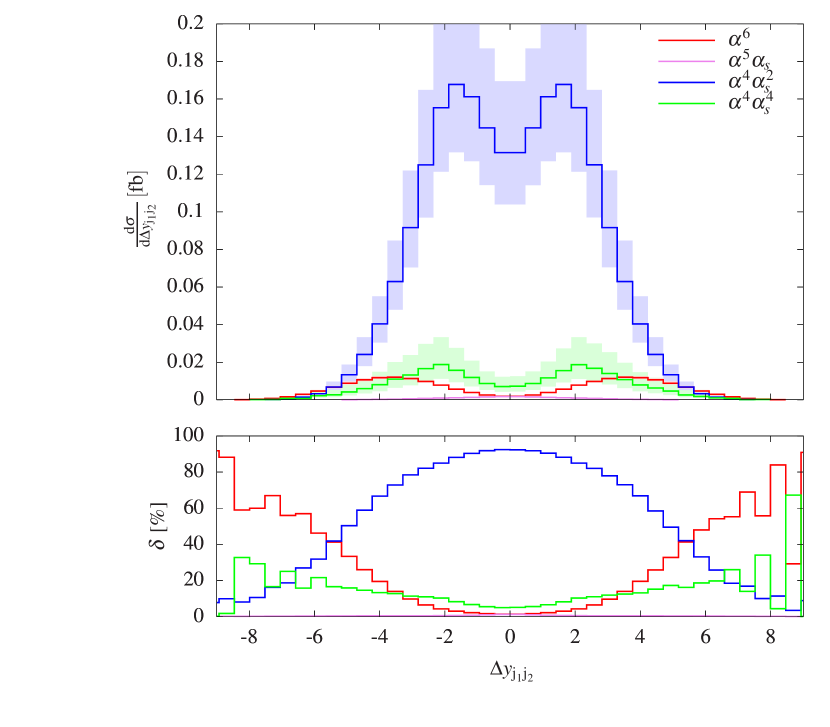
(a)

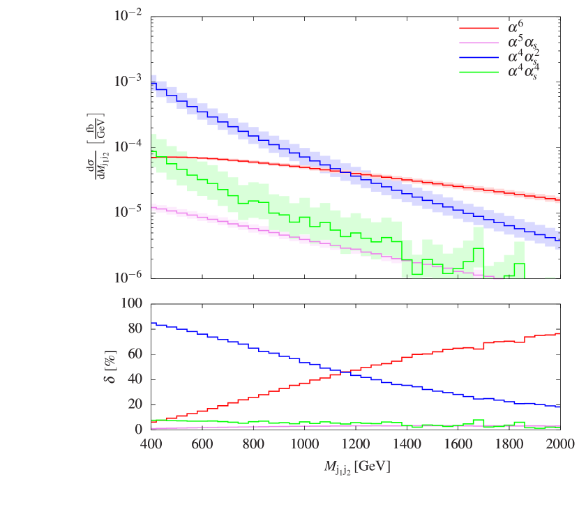
(b)

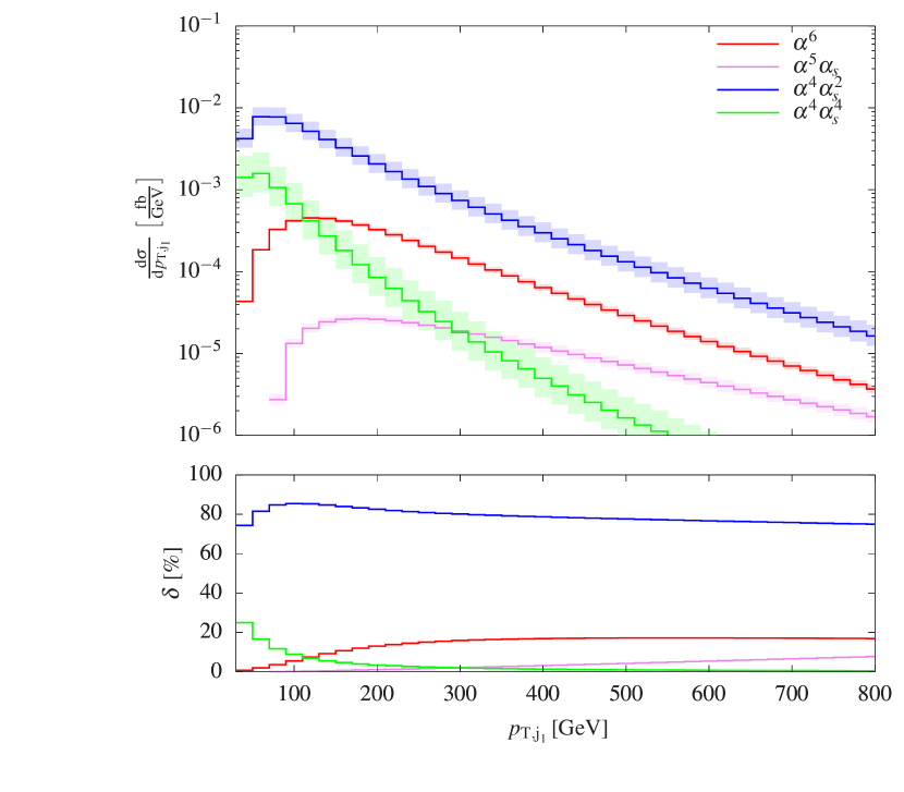
(c)

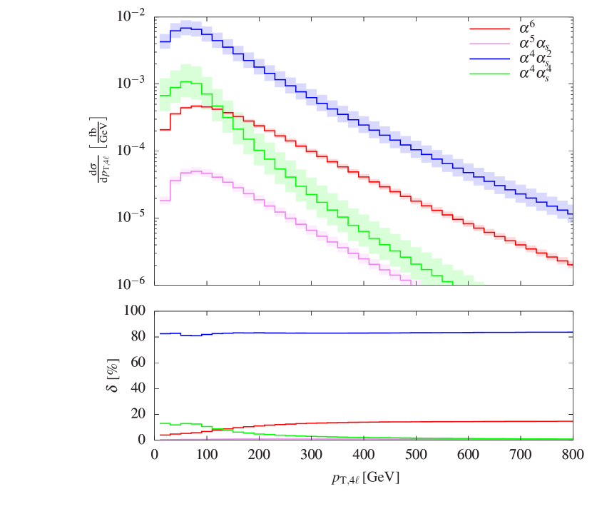
(d)

Figure 5: LO differential distributions at orders $\mathcal{O}{\left(\alpha^{6}\right)}$ (EW contribution), $\mathcal{O}{\left(\alpha_{\text{s}}\alpha^{5}\right)}$ (interference), and $\mathcal{O}{\left(\alpha_{\text{s}}^{2}\alpha^{4}\right)}$ (QCD contribution) combined with the loop-induced contribution of order $\mathcal{O}{\left(\alpha_{\text{s}}^{4}\alpha^{4}\right)}$. The upper panels show absolute predictions, while the lower ones show each contribution relative to the sum of all of them. The observables read as follows: rapidity difference between the two hardest jets (top left), invariant mass of the two hardest jets (top right), transverse momentum of the hardest jet (bottom left), and transverse momentum of the 4 leptons (bottom right).

In addition, we include predictions for the loop-induced contributions at the order $\mathcal{O}{\left(\alpha_{\text{s}}^{4}\alpha^{4}\right)}$. While the upper panels show the absolute predictions, the lower ones display each contribution relative to the sum of all of them.

The rapidity difference between the two hardest jets, shown in Figure 5(a), is a typical handle to enhance the EW contribution. As expected, the EW contribution becomes dominant only in a rather extreme part of the phase space, typically for $|\Delta y_{\text{j}_{1}\text{j}_{2}}|>5$. The central region is largely dominated by the QCD contributions which amount to more than $90\%$ of the total process. The interference contribution is below $1\%$ and hardly visible in the figure. The loop-induced process is particularly interesting. It is minimal for low rapidity difference but relatively increasing towards large rapidity difference like the EW contribution.

A further variable that is used to enhance the EW contribution is the di-jet invariant mass, whose distribution is shown in Figure 5(b). The EW contribution exceeds the QCD contribution only for $M_{\text{j}_{1}\text{j}_{2}}>1200\,\text{GeV}$. The fraction of the loop-induced contribution decreases with increasing invariant mass, while the interference increases but stays below $5\%$ for $M_{\text{j}_{1}\text{j}_{2}}<2000\,\text{GeV}$.

In Figure 5(c), the distribution in the transverse momentum of the hardest jet is shown. The relative EW contribution is slowly increasing with $p_{{\mathrm{T}},\text{j}_{1}}$ to reach almost $20\%$ at $400\,\text{GeV}$. The interference contribution becomes non negligible in this part of phase space and amounts to about $10\%$ for $p_{{\mathrm{T}},\text{j}_{1}}=800\,\text{GeV}$. Finally, the loop-induced contribution drops quickly and is below $3\%$ above $200\,\text{GeV}$.

The distribution in the transverse momentum of the four leptons, shown in Figure 5(d), behaves qualitatively similar to the distribution in the transverse momentum of the hardest jet. This is expected as these two observables are correlated. It is worth noticing that the interference contribution does not increase towards high transverse momentum as in the previous case and is thus almost imperceptible over the whole range. Also, the loop-induced contribution is dropping less quickly than in the previous case. In particular, in the first bin of the distribution in the transverse momentum of the hardest jet, the loop-induced process represents about $25\%$ of the total predictions, while here it is about $15\%$.

NLO distributions

We turn to distributions including NLO corrections. In the following figures, the upper panels show the absolute predictions for the LO EW component of $\mathcal{O}{\left(\alpha^{6}\right)}$ complemented by predictions including the orders $\mathcal{O}{\left(\alpha^{7}\right)}$ (NLO EW) or $\mathcal{O}{\left(\alpha_{\text{s}}\alpha^{6}\right)}$ (NLO QCD). In addition, the best prediction is denoted NLO EW+QCD and includes both types of corrections summed. In the lower panel, the three NLO predictions are normalised to the LO EW predictions of $\mathcal{O}{\left(\alpha^{6}\right)}$.

The observables shown in Figure 6 are related to the two hardest jets. We start with the two observables that are typically used to enhance EW contributions over its irreducible QCD background: the invariant mass (Figure 6(a)) and the rapidity difference (Figure 6(b)) of the two leading jets.

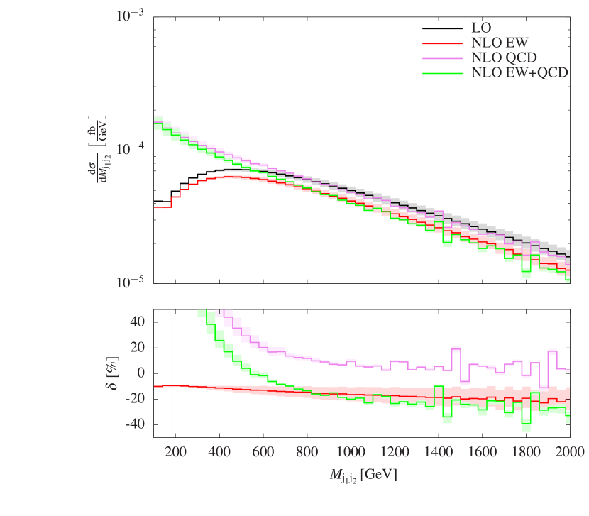
(a)

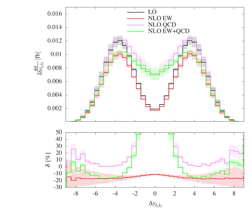
(b)

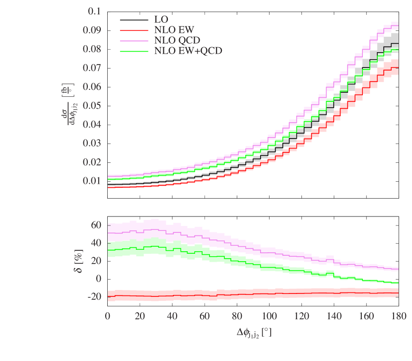
(c)

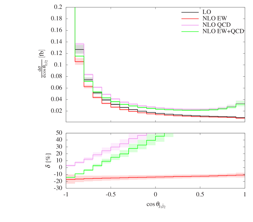
(d)

Figure 6: LO and NLO differential distributions at orders $\mathcal{O}{\left(\alpha^{6}\right)}$ (LO), $\mathcal{O}{\left(\alpha^{7}\right)}$ (NLO EW), $\mathcal{O}{\left(\alpha_{\text{s}}\alpha^{6}\right)}$ (NLO QCD), and NLO EW+QCD. The upper panels show absolute predictions while the lower ones show each contribution relative to the LO predictions. The observables read as follows: invariant mass of the two hardest jets (top left), rapidity separation of the two hardest jets (top right), azimuthal angle between the two hardest jets (bottom left), and cosine of the angle between the two hardest jets (bottom right).

The most interesting feature is that the bulk of the positive QCD corrections is located at low di-jet invariant mass. The $\mathcal{O}{\left(\alpha_{\text{s}}\alpha^{6}\right)}$ corrections are well above $100\%$ in the first bins but become of the order of a few percent above $600\,\text{GeV}$. This effect has been already observed and partially discussed in Ref. Ballestrero:2018anz for like-sign W-boson scattering and is due the appearance of W or Z bosons becoming resonant and decaying to a pair of jets when including real gluon radiation. As shown in Figures 1(g) and 1(h), $\text{p}\text{p}\to\text{e}^{+}\text{e}^{-}\mu^{+}\mu^{-}\text{j}\text{j}$ also includes contributions from triple vector-boson production (WZZ and ZZZ) at order $\mathcal{O}{\left(\alpha^{6}\right)}$. At LO, the massive vector boson decaying hadronically cannot become resonant due to the cut on the invariant mass of the two jets at $100\,\text{GeV}$ [see Eq. (10)]. When including real radiation at NLO, the cut (10) does not necessarily apply to the two quarks coming from the vector-boson decay. An extra gluon jet can make up the $M_{\text{j}_{1}\text{j}_{2}}>100\,\text{GeV}$ and allows the two quarks to originate from a resonant W or Z boson. Thus, the relatively large QCD corrections found here are a combined effect of the real radiation, the event selection, and the inclusion of tri-boson contributions. We would like to emphasise that the phase-space region of our default setup is rather inclusive and should be avoided if one does not include tri-boson contributions in the theory predictions. Otherwise, the fiducial corrections at NLO QCD will most likely be off by about $20\%$, and this offset is by no means accounted for by scale-variation uncertainties. This consideration is particularly important if Monte Carlo programs using the VBS approximation Ballestrero:2018anz are used to extrapolate measurements from the inclusive region to more VBS-enriched regions. An alternative is to subtract the on-shell tri-boson contributions from the results for the full process. Such a strategy is often used in experimental analysis to extract VBS contributions. While it allows one to claim a VBS measurement, care has to be taken not to violate gauge invariance. Furthermore, it has the disadvantage to make the measurement even more theory dependent. In our opinion, the most straightforward and physical measurement would include both the QCD and the EW processes and in the latter all possible contributions including tri-boson production, i.e. all contributions to a given physical final state. The EW corrections, on the other hand, do not display an unexpected behaviour but confirm the results known from other VBS signatures Biedermann:2016yds ; Biedermann:2017bss ; Denner:2019tmn . They become negatively large for large invariant masses owing to enhanced EW logarithms to reach $-20\%$ at $2\,\text{TeV}$.

Turning to the distribution in the rapidity difference shown in Figure 6(b), the QCD corrections reach almost $300\%$ in the central rapidity region. The rapidity separation of the two hardest jets is strongly correlated to their invariant mass (see, for instance, Figure 3 of Ref. Ballestrero:2018anz ). Thus, the arguments given for the distribution in $M_{\text{j}_{1}\text{j}_{2}}$ can be transfered to the distribution in $\Delta y_{\text{j}_{1}\text{j}_{2}}$. Events with small $\Delta y_{\text{j}_{1}\text{j}_{2}}$ are depleted at LO owing to the cut (10), while this is not the case at NLO QCD where extra gluons can provide a leading jet. The distribution also shows that a cut on the rapidity difference would be very effective in removing the sizeable QCD corrections linked to triple-vector-boson production in a similar way as a stronger cut on $M_{\text{j}_{1}\text{j}_{2}}$. Thus, the large QCD corrections could be reduced by either a cut on $\Delta y_{\text{j}_{1}\text{j}_{2}}$ or a stronger one on $M_{\text{j}_{1}\text{j}_{2}}$, which are usually imposed in VBS studies. The EW corrections are moderate and vary between $-10\%$ for zero rapidity difference and $-20\%$ for large rapidity differences.

Figures 6(c) and 6(d) show distributions in the azimuthal-angle difference and the cosine of the angle between the two leading jets, respectively, which provide information on the correlation between the two jets. The EW corrections are rather stable throughout the kinematic range and vary by less than $7\%$. For the azimuthal-angle difference, the QCD corrections are maximal near $30^{\circ}$ where they are about $55\%$. When the two jets have maximal azimuthal-angle difference, the LO contribution is maximal and receives QCD corrections at the level of $10\%$. The distribution in $\cos\theta_{\text{j}_{1}\text{j}_{2}}$ peaks at $-1$, i.e. when the two jets are back-to-back. The QCD corrections are minimal there but exceed $200\%$ when the two jets are close to each other.

In Figure 7 we display distributions related to the 4-lepton system, i.e. the Z-boson pair, and the electron–positron pair, i.e. one of the Z bosons.

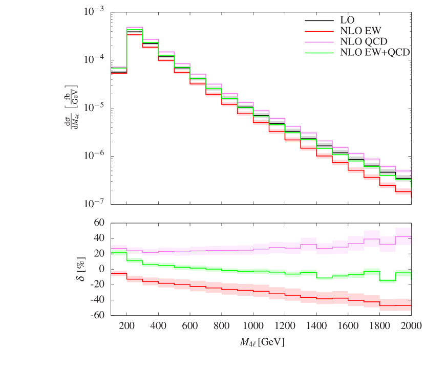
(a)

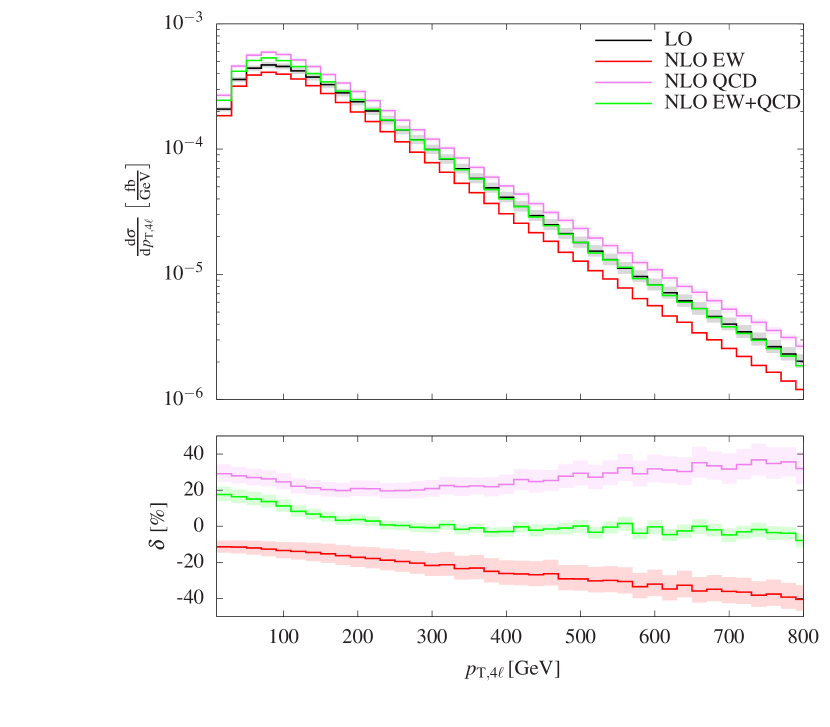
(b)

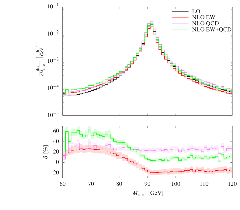
(c)

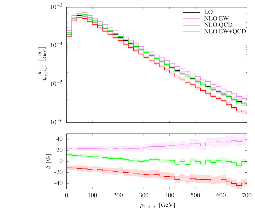
(d)

Figure 7: LO and NLO differential distributions at orders $\mathcal{O}{\left(\alpha^{6}\right)}$ (LO), $\mathcal{O}{\left(\alpha^{7}\right)}$ (NLO EW), $\mathcal{O}{\left(\alpha_{\text{s}}\alpha^{6}\right)}$ (NLO QCD), and NLO EW+QCD. The upper panels show absolute predictions while the lower ones show each contribution relative to the LO predictions. The observables read as follows: invariant mass of 4-lepton system (top left), transverse momentum of the 4 leptons (top right), invariant mass of the electron–positron system (bottom left), and transverse momentum of the electron–positron system (bottom right).

The distribution in the invariant mass of the 4-lepton system receives the typical EW Sudakov corrections growing to $-40\%$ at $M_{4\ell}=2\,\text{TeV}$. The QCD corrections increase from $20\%$ to $40\%$ in the considered range. As a consequence, the overall NLO corrections experience a cancellation for larger invariant masses and decrease from $20\%$ to almost zero towards large $M_{4\ell}$. The distribution in the transverse momentum of the 4 leptons (Figure 7(b)) is particularly interesting as it is the transverse momentum of the vector-boson scattering subprocess. The corrections behave similarly as for the distribution in the invariant mass of the 4-lepton system and show cancellations for large transverse momenta. The EW corrections steadily increase to $-40\%$ at $p_{\text{T},4\ell}=800\,\text{GeV}$. The relative QCD ones, on the other hand, reach a minimum near $200\,\text{GeV}$ and slowly increase up to $40\%$ at $800\,\text{GeV}$. The distribution in the invariant mass of the electron–positron system, presented in Figure 7(c), shows a typical Z-boson resonance. While the QCD corrections hardly modify the shape of this distribution, the EW ones exhibit a radiative tail below the resonance reaching more than $+20\%$. This tail is due to real photon radiation that takes away part of the energy of the electron–positron system and thus shifts events from the peak towards lower invariant masses. Such an effect is well known and has been observed already for Drell–Yan, di-boson, or top–anti-top production processes. The distribution in the transverse momentum of the electron–positron system, i.e. the transverse momentum of one of the Z bosons, is presented in Figure 7(d). The EW corrections increase from $-10\%$ to $-40\%$ and the QCD corrections from $25\%$ to $40\%$, leading to an overall NLO correction decreasing from $15\%$ to almost zero.

Next we study distributions in transverse momenta and rapidities of the leading jet and the positron in Figure 8.

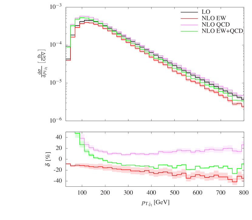
(a)

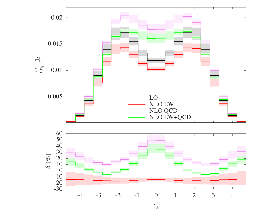
(b)

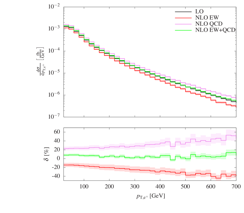
(c)

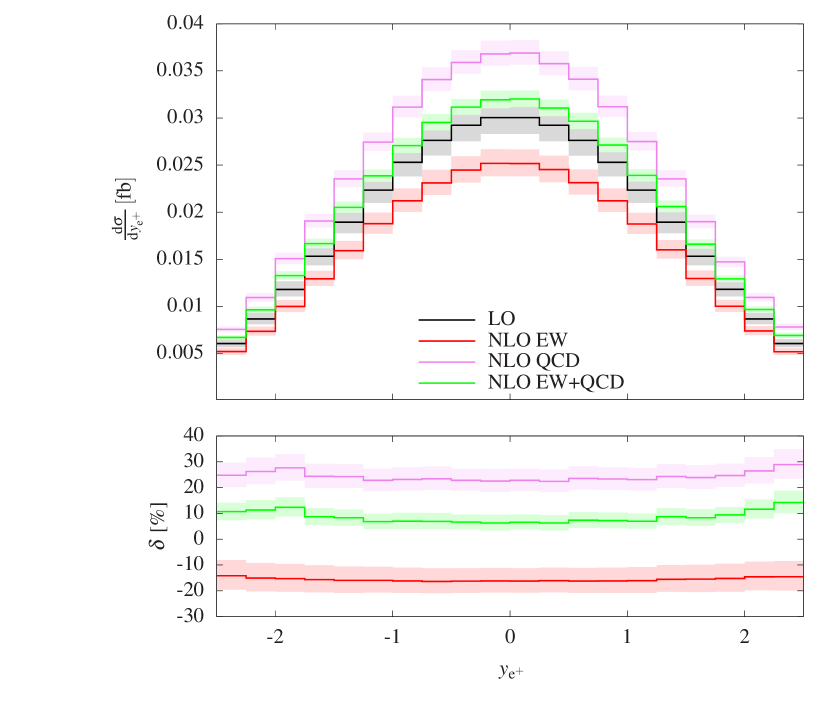
(d)

Figure 8: LO and NLO differential distributions at orders $\mathcal{O}{\left(\alpha^{6}\right)}$ (LO), $\mathcal{O}{\left(\alpha^{7}\right)}$ (NLO EW), $\mathcal{O}{\left(\alpha_{\text{s}}\alpha^{6}\right)}$ (NLO QCD), and NLO EW+QCD. The upper panels show absolute predictions while the lower ones show each contribution relative to the LO predictions. The observables read as follows: transverse momentum of the hardest jet (top left), rapidity of the hardest jet (top right), transverse momentum of the positron (bottom left), and rapidity of the positron (bottom right).

As observed in previous computations of VBS processes Biedermann:2017bss ; Denner:2019tmn , the distribution in the transverse momentum of the leading jet (Figure 8(a)) is suppressed for small transverse momenta and receives large QCD corrections in this region. This can be attributed to the presence of an extra jet and reshuffling of energy between the jets. In the rest of the spectrum, the QCD corrections are at the level of $+20\%$ as for the fiducial cross section. The EW corrections show the typical high-energy behaviour of other transverse-momentum distributions growing negatively large with increasing transverse momentum and reaching about $-40\%$ at $800\,\text{GeV}$. The distribution in the rapidity of the hardest jet (Figure 8(b)) displays a similar behaviour as the rapidity difference of the jet pair. While the relative EW corrections are rather flat, the QCD ones show large variations being maximal in the central region and in the peripheral region. At intermediate rapidity, the corrections are the lowest with a bit more than $+10\%$. The distribution in the transverse momentum of the positron (Figure 8(c)) follows closely the distribution in the transverse momentum of the electron–positron pair (Figure 7(d)), up to the region of very small transverse momentum. Both the EW and QCD corrections display the same behaviour for both distributions. The distribution in the rapidity of the positron peaks in the central region. Both QCD and EW corrections are flat.

Finally, we show distributions in angular variables related to pairs of leptons in Figure 9.

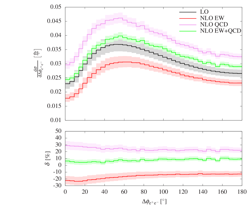
(a)

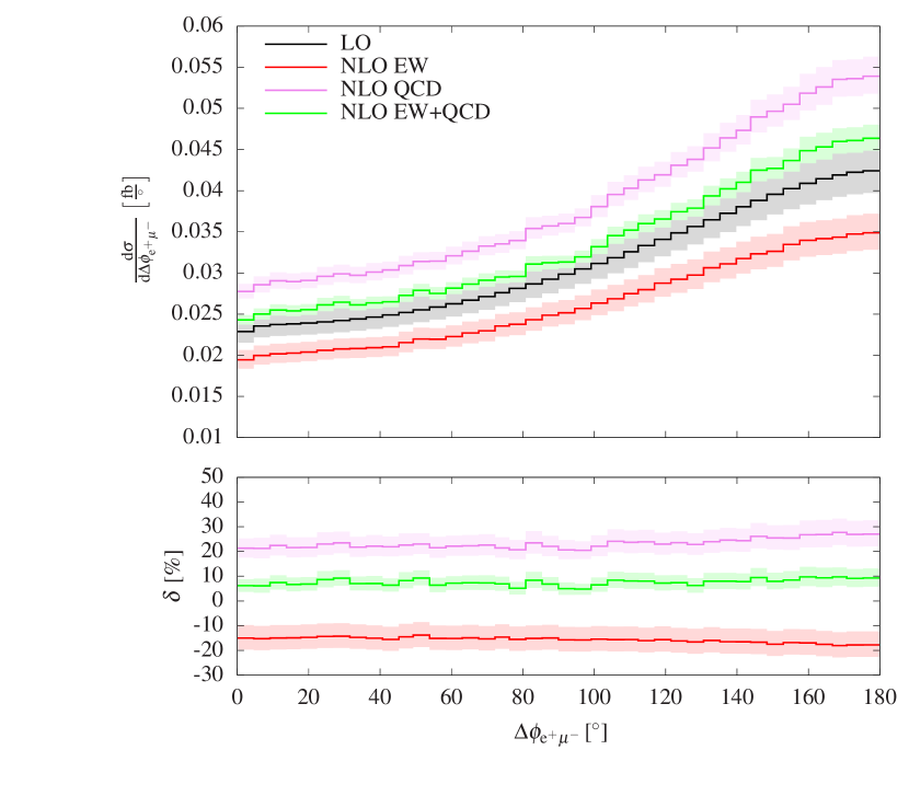
(b)

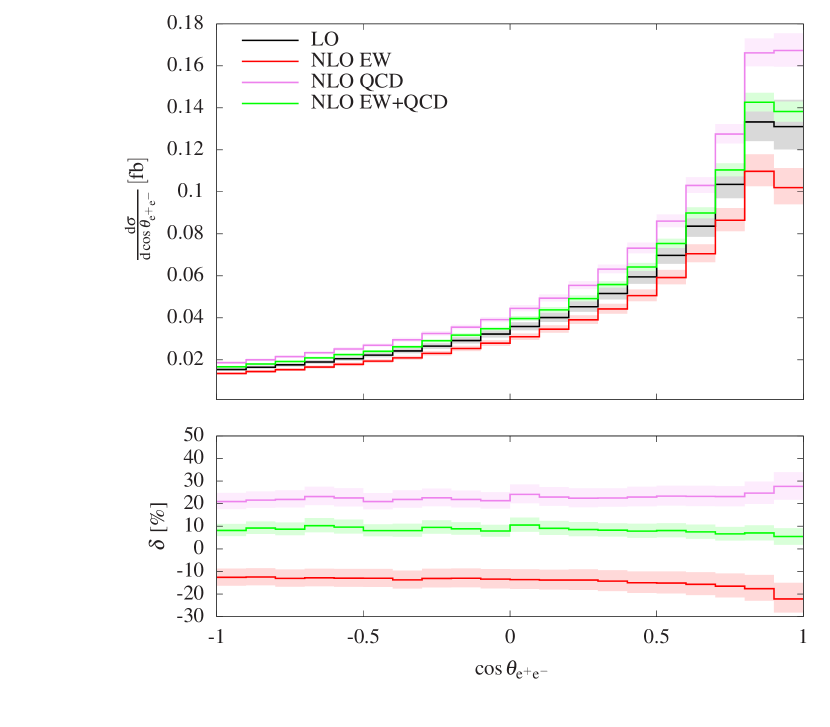
(c)

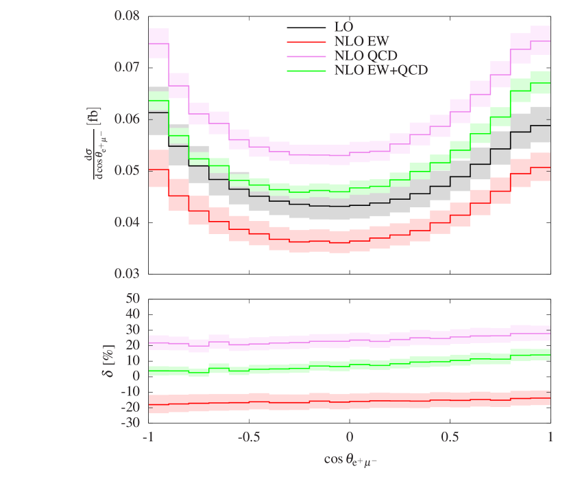
(d)

Figure 9: LO and NLO differential distributions at orders $\mathcal{O}{\left(\alpha^{6}\right)}$ (LO), $\mathcal{O}{\left(\alpha^{7}\right)}$ (NLO EW), $\mathcal{O}{\left(\alpha_{\text{s}}\alpha^{6}\right)}$ (NLO QCD), and NLO EW+QCD. The upper panels show absolute predictions while the lower ones show each contribution relative to the LO predictions. The observables read as follows: azimuthal angle between the electron and the positron (top left), azimuthal angle between the positron and the muon (top right), cosine of the angle between the electron and the positron (bottom left), and cosine of the angle between the positron and the muon (bottom right).

Such observables are particularly useful in ZZ scattering as they give insight in details of the scattering process which is not possible for other VBS signatures due to the presence of neutrino(s). We start with distributions in azimuthal-angle differences for the electron–positron system (Figure 9(a)) and the positron–muon system (Figure 9(b)). Given the flavour, the first observable relates two opposite-sign leptons originating from the same Z-boson decay, while the second one links leptons of two different Z-boson decays. The shapes of the two distributions are therefore rather different. The distribution for the electron–positron system peaks near $50^{\circ}$, while the one for the positron–muon case is maximal at $180^{\circ}$. The corrections behave also rather differently. In the electron–positron case, the QCD (EW) corrections are maximally positive (negative) at low angle, leading to an overall correction which is rather stable around $+10\%$ over the whole spectrum. For the positron–muon azimuthal separation, the QCD corrections slightly increase by almost ten percent from low to large angles, while the EW ones have the opposite trend. Thus, the overall corrections are again rather steady at about $10\%$. We emphasise that such cancellations are, a priori, largely accidental and should not be taken for granted in other VBS signatures or setups. The last two distributions concern the cosine of the angle between the two leptons for the same two leptonic systems (Figures 9(c) and 9(d)). It is interesting to notice that for these distributions, again both types of corrections do not induce large shape distortions (less than $10\%$). This makes such observables particularly attractive for correlation analysis or to test models of new physics.

4 Conclusion

In this article we have presented a calculation of the NLO EW and QCD corrections of orders $\mathcal{O}{\left(\alpha^{7}\right)}$ and $\mathcal{O}{\left(\alpha_{\text{s}}\alpha^{6}\right)}$, respectively, for the process $\text{p}\text{p}\to\text{e}^{+}\text{e}^{-}\mu^{+}\mu^{-}\text{j}\text{j}+X$. Our results include, in particular, the NLO EW and QCD corrections to the LO EW contribution of order $\mathcal{O}{\left(\alpha^{6}\right)}$, which is dominated by vector-boson scattering (VBS) into a pair of Z bosons. As the full matrix elements are used at the corresponding orders, our computation accounts for all off-shell, non-resonant, and interference effects. In particular, triple-boson-production processes are part of the EW contributions. We have included all partonic channels apart from those involving initial-state bottom quarks or photons, which are suppressed.

The EW corrections of order $\mathcal{O}{\left(\alpha^{7}\right)}$ are found to be relatively large, in agreement with similar results obtained previously for $\text{W}^{\pm}\text{W}^{\pm}$ and WZ scattering and the expectation that large EW corrections are an intrinsic feature of VBS at the LHC. For the chosen fiducial cross section, the corrections are $-16\%$ and can be well reproduced by a simple logarithmic approximation. In the high-energy tails of distributions the EW corrections can reach $-40\%$. The QCD corrections of order $\mathcal{O}{\left(\alpha_{\text{s}}\alpha^{6}\right)}$ exceed $20\%$ for the fiducial cross section. While such a magnitude for QCD corrections at the LHC is perfectly normal, it is rather large for VBS processes. In particular, previous computations relying on the VBS approximation have found QCD corrections at the percent level, in strong contrast to our findings. These differences are due to the fact that our computation is done for a rather inclusive phase-space region ($M_{\text{j}_{1}\text{j}_{2}}>100\,\text{GeV}$ as opposed to $M_{\text{j}_{1}\text{j}_{2}}\;\raisebox{-3.00003pt}{$\stackrel{{\scriptstyle\displaystyle>}}{{\sim}}$}\;500\,\text{GeV}$ and/or $\Delta y_{\text{j}_{1}\text{j}_{2}}\;\raisebox{-3.00003pt}{$\stackrel{{\scriptstyle\displaystyle>}}{{\sim}}$}\;3$ usually) and includes tri-boson contributions. Hence, when including real QCD radiation at NLO, Z or W bosons decaying hadronically can become resonant thus leading to very large corrections that are not captured by scale variation. We emphasise that there is nothing wrong in using such inclusive fiducial regions as long as the theoretical simulations used include tri-boson contributions at NLO QCD. In particular, Monte Carlo programs relying on the VBS approximation should not be used to extrapolate measurements from the inclusive region to more VBS-enriched regions. Nonetheless, they still constitute reliable theoretical predictions in the typical VBS regions (with $M_{\text{j}_{1}\text{j}_{2}}\;\raisebox{-3.00003pt}{$\stackrel{{\scriptstyle\displaystyle>}}{{\sim}}$}\;500\,\text{GeV}$ and/or $\Delta y_{\text{j}_{1}\text{j}_{2}}\;\raisebox{-3.00003pt}{$\stackrel{{\scriptstyle\displaystyle>}}{{\sim}}$}\;3$), where the NLO QCD corrections are of the usual size. The present work also shows that the proper inclusion of tri-boson contributions is of great relevance. We strongly advocate for simpler and more physical measurements where tri-boson contributions are not subtracted from the signal. This has the advantage to be clearly gauge invariant and not to rely on conventions and theory predictions. Finally, as argued in previous work, comparing predictions including all QCD, interference, and EW contributions with the measurements is the cleanest way of testing the SM in such processes.

We have also analysed the composition of the LO process by comparing contributions at orders: $\mathcal{O}{\left(\alpha^{6}\right)}$ (EW contribution), $\mathcal{O}{\left(\alpha_{\text{s}}\alpha^{5}\right)}$ (interference), and $\mathcal{O}{\left(\alpha_{\text{s}}^{2}\alpha^{4}\right)}$ (QCD contribution). The findings are in line with known observations that VBS ZZ is a challenging channel due to the very large irreducible QCD background. In particular, in the fiducial region chosen, the LO EW contributions amount to less than $10\%$. In the LO analysis, we have also further included the loop-induced contribution with gluon–gluon initial state at order $\mathcal{O}{\left(\alpha_{\text{s}}^{4}\alpha^{4}\right)}$. It has been found to be of the order of $10\%$ in the fiducial region, but becomes relatively negligible in the high-energy limit of differential distributions. Imposing an extra VBS cut $M_{\text{j}_{1}\text{j}_{2}}>500\,\text{GeV}$ enhances the EW contribution to more than $30\%$.

We would like to point out that this calculation constitutes a further leap in complexity with respect to previous calculations for VBS processes. The fact that eight charged external particles occur increases significantly the complexity of the virtual and, in particular, of the real corrections. The number of partonic channels is amplified by a factor of 5 with respect to like-sign W scattering and 1.5 relative to WZ scattering. As a consequence, the required CPU time is increased and efficient book-keeping, automation and parallelisation are crucial.

Finally, we hope that these results will be useful in the current and upcoming measurements of ZZ VBS at the LHC. In particular, we believe that this article contains valuable information for the experimental collaborations when conducting their analysis.

References

- (1) ATLAS Collaboration, G. Aad et al., Evidence for Electroweak Production of in Collisions at TeV with the ATLAS Detector, Phys. Rev. Lett. 113 (2014) 141803, [arXiv:1405.6241].
- (2) CMS Collaboration, V. Khachatryan et al., Study of vector boson scattering and search for new physics in events with two same-sign leptons and two jets, Phys. Rev. Lett. 114 (2015) 051801, [arXiv:1410.6315].
- (3) ATLAS Collaboration, M. Aaboud et al., Measurement of vector-boson scattering and limits on anomalous quartic gauge couplings with the ATLAS detector, Phys. Rev. D96 (2017) 012007, [arXiv:1611.02428].
- (4) CMS Collaboration, A. M. Sirunyan et al., Observation of electroweak production of same-sign W boson pairs in the two jet and two same-sign lepton final state in proton-proton collisions at TeV, Phys. Rev. Lett. 120 (2018) 081801, [arXiv:1709.05822].
- (5) ATLAS Collaboration, M. Aaboud et al., Observation of electroweak boson pair production in association with two jets in collisions at TeV with the ATLAS detector, Phys. Lett. B 793 (2019) 469–492, [arXiv:1812.09740].
- (6) CMS Collaboration, A. M. Sirunyan et al., Measurement of electroweak WZ boson production and search for new physics in WZ + two jets events in pp collisions at TeV, Phys. Lett. B 795 (2019) 281–307, [arXiv:1901.04060].
- (7) ATLAS Collaboration, M. Aaboud et al., Observation of electroweak production of a same-sign boson pair in association with two jets in collisions at TeV with the ATLAS detector, Phys. Rev. Lett. 123 (2019) 161801, [arXiv:1906.03203].
- (8) CMS Collaboration, A. M. Sirunyan et al., Measurements of production cross sections of WZ and same-sign WW boson pairs in association with two jets in proton-proton collisions at TeV, arXiv:2005.01173.
- (9) CMS Collaboration, A. M. Sirunyan et al., Measurement of vector boson scattering and constraints on anomalous quartic couplings from events with four leptons and two jets in proton-proton collisions at TeV, Phys. Lett. B774 (2017) 682–705, [arXiv:1708.02812].
- (10) ATLAS Collaboration, G. Aad et al., Observation of electroweak production of two jets and a -boson pair with the ATLAS detector at the LHC, arXiv:2004.10612.
- (11) CMS Collaboration, A. M. Sirunyan et al., Evidence for electroweak production of four charged leptons and two jets in proton-proton collisions at TeV, arXiv:2008.07013.
- (12) CMS Collaboration, A. M. Sirunyan et al., Search for anomalous electroweak production of vector boson pairs in association with two jets in proton-proton collisions at 13 TeV, Phys. Lett. B 798 (2019) 134985, [arXiv:1905.07445].
- (13) ATLAS Collaboration, G. Aad et al., Search for the electroweak diboson production in association with a high-mass dijet system in semileptonic final states in collisions at TeV with the ATLAS detector, Phys. Rev. D 100 (2019) 032007, [arXiv:1905.07714].
- (14) J. Baglio et al., Release Note - VBFNLO 2.7.0, arXiv:1404.3940.
- (15) M. Rauch, Vector-Boson Fusion and Vector-Boson Scattering, arXiv:1610.08420.
- (16) B. Biedermann, A. Denner, and M. Pellen, Large electroweak corrections to vector-boson scattering at the Large Hadron Collider, Phys. Rev. Lett. 118 (2017) 261801, [arXiv:1611.02951].
- (17) B. Biedermann, A. Denner, and M. Pellen, Complete NLO corrections to W+W+ scattering and its irreducible background at the LHC, JHEP 10 (2017) 124, [arXiv:1708.00268].
- (18) A. Denner, S. Dittmaier, P. Maierhöfer, M. Pellen, and C. Schwan, QCD and electroweak corrections to WZ scattering at the LHC, JHEP 06 (2019) 067, [arXiv:1904.00882].
- (19) M. Chiesa, A. Denner, J.-N. Lang, and M. Pellen, An event generator for same-sign W-boson scattering at the LHC including electroweak corrections, Eur. Phys. J. C 79 (2019) 788, [arXiv:1906.01863].
- (20) CMS Collaboration, Vector Boson Scattering prospective studies in the ZZ fully leptonic decay channel for the High-Luminosity and High-Energy LHC upgrades, Tech. Rep. CMS-PAS-FTR-18-014, CERN, Geneva, 12, 2018.
- (21) B. Jäger, C. Oleari, and D. Zeppenfeld, Next-to-leading order QCD corrections to Z boson pair production via vector-boson fusion, Phys. Rev. D 73 (2006) 113006, [hep-ph/0604200].
- (22) B. Jäger, A. Karlberg, and G. Zanderighi, Electroweak production in the Standard Model and beyond in the POWHEG-BOX V2, JHEP 03 (2014) 141, [arXiv:1312.3252].
- (23) S. Alioli, P. Nason, C. Oleari, and E. Re, A general framework for implementing NLO calculations in shower Monte Carlo programs: the POWHEG BOX, JHEP 06 (2010) 043, [arXiv:1002.2581].
- (24) F. Campanario, M. Kerner, L. D. Ninh, and D. Zeppenfeld, Next-to-leading order QCD corrections to ZZ production in association with two jets, JHEP 07 (2014) 148, [arXiv:1405.3972].
- (25) C. Li, et al., Loop-induced production at the LHC: an improved description by matrix-element matching, arXiv:2006.12860.
- (26) S. Catani and M. H. Seymour, A general algorithm for calculating jet cross-sections in NLO QCD, Nucl. Phys. B485 (1997) 291–419, [hep-ph/9605323]. [Erratum: Nucl. Phys. B510 (1998) 503].
- (27) S. Dittmaier, A general approach to photon radiation off fermions, Nucl. Phys. B565 (2000) 69–122, [hep-ph/9904440].
- (28) S. Dittmaier, A. Kabelschacht, and T. Kasprzik, Polarized QED splittings of massive fermions and dipole subtraction for non-collinear-safe observables, Nucl. Phys. B800 (2008) 146–189, [arXiv:0802.1405].
- (29) A. Denner, S. Dittmaier, M. Pellen, and C. Schwan, Low-virtuality photon transitions and the photon-to-jet conversion function, Phys. Lett. B 798 (2019) 134951, [arXiv:1907.02366].
- (30) F. A. Berends, R. Pittau, and R. Kleiss, All electroweak four fermion processes in electron-positron collisions, Nucl. Phys. B424 (1994) 308–342, [hep-ph/9404313].
- (31) A. Denner, S. Dittmaier, M. Roth, and D. Wackeroth, Predictions for all processes fermions , Nucl. Phys. B560 (1999) 33–65, [hep-ph/9904472].
- (32) S. Dittmaier and M. Roth, LUSIFER: A LUcid approach to six FERmion production, Nucl. Phys. B642 (2002) 307–343, [hep-ph/0206070].
- (33) S. Actis, A. Denner, L. Hofer, A. Scharf, and S. Uccirati, Recursive generation of one-loop amplitudes in the Standard Model, JHEP 04 (2013) 037, [arXiv:1211.6316].
- (34) S. Actis et al., RECOLA: REcursive Computation of One-Loop Amplitudes, Comput. Phys. Commun. 214 (2017) 140–173, [arXiv:1605.01090].
- (35) A. Denner, S. Dittmaier, and L. Hofer, Collier - A fortran-library for one-loop integrals, PoS LL2014 (2014) 071, [arXiv:1407.0087].
- (36) A. Denner, S. Dittmaier, and L. Hofer, COLLIER: a fortran-based Complex One-Loop LIbrary in Extended Regularizations, Comput. Phys. Commun. 212 (2017) 220–238, [arXiv:1604.06792].
- (37) G. ’t Hooft and M. J. G. Veltman, Scalar one loop integrals, Nucl. Phys. B153 (1979) 365–401.
- (38) W. Beenakker and A. Denner, Infrared divergent scalar box integrals with applications in the electroweak Standard Model, Nucl. Phys. B338 (1990) 349–370.
- (39) S. Dittmaier, Separation of soft and collinear singularities from one-loop N-point integrals, Nucl. Phys. B675 (2003) 447–466, [hep-ph/0308246].
- (40) A. Denner and S. Dittmaier, Scalar one-loop 4-point integrals, Nucl. Phys. B844 (2011) 199–242, [arXiv:1005.2076].
- (41) G. Passarino and M. J. G. Veltman, One-loop corrections for annihilation into in the Weinberg Model, Nucl. Phys. B160 (1979) 151.
- (42) A. Denner and S. Dittmaier, Reduction of one-loop tensor 5-point integrals, Nucl. Phys. B658 (2003) 175–202, [hep-ph/0212259].
- (43) A. Denner and S. Dittmaier, Reduction schemes for one-loop tensor integrals, Nucl. Phys. B734 (2006) 62–115, [hep-ph/0509141].
- (44) A. Ballestrero et al., Precise predictions for same-sign W-boson scattering at the LHC, Eur. Phys. J. C78 (2018) 671, [arXiv:1803.07943].
- (45) M. Pellen, Exploring the scattering of vector bosons at LHCb, Phys. Rev. D101 (2020) 013002, [arXiv:1908.06805].
- (46) B. Biedermann, et al., Automation of NLO QCD and EW corrections with Sherpa and Recola, Eur. Phys. J. C77 (2017) 492, [arXiv:1704.05783].
- (47) S. Bräuer, A. Denner, M. Pellen, M. Schönherr, and S. Schumann, Fixed-order and merged parton-shower predictions for WW and WWj production at the LHC including NLO QCD and EW corrections, arXiv:2005.12128.
- (48) Z. Nagy and Z. Trocsanyi, Next-to-leading order calculation of four-jet observables in electron-positron annihilation, Phys. Rev. D59 (1999) 014020, [hep-ph/9806317]. [Erratum: Phys. Rev. D62 (2000) 099902].
- (49) A. Denner, S. Dittmaier, M. Roth, and L. H. Wieders, Electroweak corrections to charged-current 4 fermion processes: Technical details and further results, Nucl. Phys. B724 (2005) 247–294, [hep-ph/0505042]. [Erratum: Nucl. Phys. B854 (2012) 504].
- (50) A. Denner and S. Dittmaier, The complex-mass scheme for perturbative calculations with unstable particles, Nucl. Phys. Proc. Suppl. 160 (2006) 22–26, [hep-ph/0605312].
- (51) NNPDF Collaboration, R. D. Ball et al., Parton distributions for the LHC Run II, JHEP 04 (2015) 040, [arXiv:1410.8849].
- (52) NNPDF Collaboration, V. Bertone, S. Carrazza, N. P. Hartland, and J. Rojo, Illuminating the photon content of the proton within a global PDF analysis, SciPost Phys. 5 (2018) 008, [arXiv:1712.07053].
- (53) J. R. Andersen et al., Les Houches 2013: Physics at TeV Colliders: Standard Model Working Group Report, arXiv:1405.1067.
- (54) A. Buckley, et al., LHAPDF6: parton density access in the LHC precision era, Eur. Phys. J. C75 (2015) 132, [arXiv:1412.7420].
- (55) A. Denner, S. Dittmaier, M. Roth, and D. Wackeroth, Electroweak radiative corrections to 4 fermions in double pole approximation: The RACOONWW approach, Nucl. Phys. B587 (2000) 67–117, [hep-ph/0006307].
- (56) ParticleDataGroup Collaboration, M. Tanabashi et al., Review of Particle Physics, Phys. Rev. D98 (2018) 030001.
- (57) LHC Higgs Cross Section Working Group Collaboration, J. R. Andersen et al., Handbook of LHC Higgs Cross Sections: 3. Higgs Properties, arXiv:1307.1347. CERN-2013-004.
- (58) D. Yu. Bardin, A. Leike, T. Riemann, and M. Sachwitz, Energy-dependent width effects in -annihilation near the Z-boson pole, Phys. Lett. B206 (1988) 539–542.
- (59) M. Cacciari, G. P. Salam, and G. Soyez, The anti- jet clustering algorithm, JHEP 04 (2008) 063, [arXiv:0802.1189].
- (60) A. Denner and S. Pozzorini, One loop leading logarithms in electroweak radiative corrections. 1. Results, Eur. Phys. J. C18 (2001) 461–480, [hep-ph/0010201].
- (61) E. Accomando, A. Denner, and S. Pozzorini, Logarithmic electroweak corrections to , JHEP 03 (2007) 078, [hep-ph/0611289].