Time-Varying Parameters as Ridge Regressions

Abstract

Time-varying parameters (TVPs) models are frequently used in economics to capture structural change. I highlight a rather underutilized fact—that these are actually ridge regressions. Instantly, this makes computations, tuning, and implementation much easier than in the state-space paradigm. Among other things, solving the equivalent dual ridge problem is computationally very fast even in high dimensions, and the crucial "amount of time variation" is tuned by cross-validation. Evolving volatility is dealt with using a two-step ridge regression. I consider extensions that incorporate sparsity (the algorithm selects which parameters vary and which do not) and reduced-rank restrictions (variation is tied to a factor model). To demonstrate the usefulness of the approach, I use it to study the evolution of monetary policy in Canada using large time-varying local projections. The application requires the estimation of about 4 600 TVPs, a task well within the reach of the new method.

1 Introduction

Economies change. Intuitively, this should percolate to the parameters of models characterizing them. To econometrically achieve that, a popular approach is Time-Varying Parameters (TVPs), where a linear equation’s coefficients follow stochastic processes — usually random walks. Classic papers in the literature consider TVP Vector Auto Regressions (TVP-VARs) to study changing monetary policy (Primiceri,, 2005) and evolving inflation dynamics (Cogley and Sargent,, 2001, 2005). Recently, such ideas were introduced to jorda2005’s local projections (LPs) to obtain directly time-varying impulse response functions (ruisi2019time; lusompa2020local).

In both the VAR and LP cases, important practical obstacles reduce the scope and applicability of TVPs. One is prohibitive computations limiting the model’s size. Another is the difficulty of tuning the crucial amount of time variation. To address those and other problems, I fully leverage the underutilized fact that TVP models are ridge regressions (RR). The connection is useful: 50 years (hoerl1970ridge) of RR widespread use, research and wisdom is readily transferable to TVPs. Among other things, this provides fast computations via a closed-form dual solution only using matrix operations. The amount of time variation is automatically tuned by cross-validation (CV). Adjustments for evolving residuals’ volatility and heterogeneous parameter drifting speeds (random walk variances) are implemented via a 2-step ridge regression (henceforth 2SRR) the flagship model of this paper. In contrast with the usual Bayesian machinery, it is easy to implement and to operate. For instance, it will never face initialization and convergence issues since it avoids altogether MCMC simulations and filtering. Moreover, the setup is directly extendable to deploy additional shrinkage schemes (sparse TVP, reduced rank TVPs) recently proposed in the literature (stevanovic2016common; bitto2018achieving). For the remainder of this introduction, I review the issues facing current TVP models, survey their related literature, and explain how the ridge approach can help.

Computations. Using standard implementations allowing for stochastic volatility (SV) in TVP-VARs, researchers are limited to a few lags and a small number of variables (not more than 4 or 5) (kilian2017SVAR). This constraint leaves the reader ever-wondering whether time variation is not merely the byproduct of omitted variables. A similar problem occurs if one wants to study time-varying local projections of a certain size, which imply repeated estimation over many horizons. Consequently, a growing number of contributions attempt to deal with the computational problem. In the state-space paradigm, koop2013large and huber2020bayesian proposed approximations to speed up MCMC simulations. giraitis2014inference and kapetanios2017large drop the state-space paradigm altogether in favor of a nonparametric kernel-based estimator. chen2012testing consider a similar approach to develop a test for smooth structural change while petrova2016quasi develops a Bayesian version particularly apt with large multivariate systems. While this type of framework allows the estimation of the desired big models, it is unclear how we can incorporate useful features such as heterogeneous variances for parameters (as in primiceri2005). Further, there seems to be an artificial division between nonparametric and law-of-motion approaches. Later, by showing that random walk TVPs give rise to a ridge regression (which will also be a smoothing splines problem), it will become clear that random walks TVPs are no less nonparametric than TVPs obtained from the "nonparametric approach". Yet, RR implements nearly the same model as classical TVP models and preserves the interpretation of the resulting coefficients as latent stochastic states. Keeping alive the parallel to a law of motion has some advantages — like an obvious prediction for tomorrow’s coefficients.

Tuning and Forecasting. On the forecasting front, AAG2013, BaumeisterKilian2014 and pettenuzzo2017forecasting have all investigated, with varying angles, the usefulness of time variation to increase prediction accuracy. A critical choice underlying forecasting successes and failures is the amount of time variation. Notoriously, tuning parameter(s) determining it can largely influence prediction results and estimated coefficients, accounting for much of the cynicism regarding the transparency and reliability of TVP models. amir2018choosing and cadonna2020triple propose to treat those pivotal hyperparameters as another layer of parameters to be estimated within the Bayesian procedure — and find this indeed helps. By showing the TVP–RR equivalence, this paper defines even more clearly what the fundamental tuning problem is for this class of models. TVP models are standard (very) high-dimensional regressions which need to be regularized somehow. By construction, the unique ridge tuning parameter, in this context, (golub1979gcv) mechanically corresponds to a ratio of two variances, that of parameter innovations and that of residuals. Hence, tuning $\lambda$ via standard (and fast) cross-validation techniques delivers the desired quantity of how much time variation there is in the coefficients. Given how the quantity is paramount for both predictive accuracy and economic analysis, it is particularly comforting that it suddenly can be tuned the same way ridge $\lambda$’s have been tuned for decades.

Fancier Shrinkage. TVP models are densely parametrized which makes overfitting an enduring threat The RR approach makes this explicit: TVP models are linear regressions where parameters always outnumber observations — and by a lot. Precisely, the ratio of parameters to observations is always $K$, the number of original regressors. Clearly, things do get any better with large models. Assuming a random walk as a law of motion and enforcing it with a varying degree of rigidity (using $\lambda$ in my approach) curbs overfitting, provided the plain constant-coefficient models itself does not overfit. However, an unpleasant side effect of $\lambda$ "abuse" is that time variation itself is evacuated. Since this problem pertains to the class of models rather than the estimation method, I borrow insights from the recent literature to extend my framework into two directions. Firstly, I consider Sparse TVPs. This means that not all parameters are created equal: some will vary and some will not. This brings hope for larger models. If adding regressors actually make some other coefficients time-invariant, we are gaining degrees of freedom. In that spirit, belmonte2014hierarchical, korobilis2014data, bitto2018achieving, cadonna2020triple, and hauzenberger2020dynamic have proposed such extensions to MCMC-based procedures. In the RR setup, this amounts to the development of the Group Lasso Ridge Regression (GLRR) which is shown to be obtainable by simply iterating 2SRR. Secondly, another natural way to discipline TVPs is to impose a factor structure. This means that instead of trying to filter, say, 20 independent states, we can span these with a parsimonious set of latent factors. This extension is considered in stevanovic2016common, dewindgambetti2014 and chan-ftvp2018. Such reduced rank restrictions are brought to this paper’s arsenal by developing a Generalized Reduced Rank Ridge Regression (GRRRR).

Results. I first evaluate the method with simulations. For models of smaller size, where traditional Bayesian procedures can also be used, 2SRR does as well and sometimes better at recovering the true parameter path than the (Bayesian) TVP-VAR. This is true whether SV is involved or not. This is practical given that running and tuning 2SRR for such small models (300 observations, 6 TVPs per equation) takes less than 5 seconds to compute. Since large single equations will be at the heart of the forecasting and empirical application, I also benchmark with with a state-of-the-art single equation Bayesian method (cadonna2020triple) that (i) optimizes the amount of shrinkage and (ii) can work in modestly higher dimensions with an acceptable computing time. Again, 2SRR provides estimates of comparable quality at a fraction of the computational cost. Additionally, I evaluate the performance of 3 variants of the RR approach in a substantive forecasting experiment. 2SRR and its iterated extension provide sizable gains for interest rates and inflation, two variables traditionally associated with the need for time variation. I complete with an application to estimating large time-varying LPs (more than 4 600 TVPs) in a Canadian context using champagnesekkel2018’s narrative monetary policy (MP) shocks. It is found that MP shocks long-run impact on inflation increased substantially starting from the 1990s (onset of inflation targeting), whereas the effects on real activity indicators (GDP, unemployment) became milder.

Intended Use. The method has comparative advantages and disadvantages. It provides quick and off-the-shelf estimates of time-varying coefficients for models of various sizes without sacrificing reliability. In fact, it sometimes increases it with respect to more sophisticated methods. This practicality and scalability make it a handy generic tool in the applied econometrician’s arsenal, for both forecasting and analysis. Additionally, the basis expansion and reparametrization ideas developed in the paper can be used to easily induce random walk parameters in models with implicit ridge shrinkage like neural network models with early stopping (MDTM; HNN). What it does not do as readily as Bayesian methods is providing inference. While it is surely can be done given that RR is equivalently a plain Bayesian regression, the paper focuses on point estimates and applications to multiple single equation modeling (like local projections or vast direct forecasting exercises). In sum, 2SRR and its variants are not built with the ambition of redeeming all the time-varying parameters models, but simply to excel in key aspects of empirical practice where current offerings have significant limitations.

Outline. Section 2 presents the ridge approach, its extensions, and related practical issues. Sections 3 and 4 report simulations and forecasting results, respectively. Section 5 applies 2SRR to (large) time-varying LPs. Tables, additional graphs and technical details are in the Appendix.

Notation. $\beta_{t,k}$ refers to the coefficient on regressor $X_{k}$ at time $t$. To make things lighter, $\beta_{t}\in{\rm I\!R}^{K}$ or $\beta_{0}\in{\rm I\!R}^{K}$ always refers to all coefficients at time $t$ or time zero, respectively. Analogously, $\beta_{k}$ represents the whole time path for the coefficient on $X_{k}$. $\boldsymbol{\beta}\in{\rm I\!R}^{KT}$ is stacking all $\beta_{k}$’s one after the other, for $k=1,...,K$. All this also applies to $u$ and $\theta$.

2 Time-Varying Parameters are Ridge Regressions

2.1 A Useful Observation

Consider a generic linear model with random walk time-varying parameters

$$y_{t} =X_{t}{\beta_{t}}+{\epsilon_{t}},\quad{\epsilon}_{t}\sim{N(0,\sigma_{\epsilon_{t}}^{2}})$$ (1a)

$${\beta_{t}} ={\beta_{t-1}}+{u}_{t},\quad{u}_{t}\sim{N(0,\Omega_{u}})$$ (1b)

where $\beta_{t}\in{\rm I\!R}^{K}$, $X_{t}^{\prime}\in{\rm I\!R}^{K}$, $u_{t}\in{\rm I\!R}^{p}$ and both $y_{t}$ and $\epsilon_{t}$ are scalars. This paper first considers a general single equation time series model and then discuss its generalization to the multivariate case in section 2.4.4. For clarity, a single equation in a VAR with $M$ variables and $P$ lags has $K=PM+1$ parameters for each equation. For simplicity of exposition, I first impose $\Omega_{u}=\sigma_{u}^{2}I_{K}$ and $\sigma_{\epsilon_{t}}^{2}=\sigma_{\epsilon}^{2}\quad\forall t$. This means all parameters are assumed to vary equally a priori and constant variance of residuals. These assumptions will be relaxed in section (2.4). The textbook way of estimating (1) is to impose some value for $\frac{\sigma_{\epsilon}}{\sigma_{u}}$ and use the Kalman filter for linear Gaussian model (hamilton1994). The advantages of the newly proposed methods will be more apparent when considering complications typically encountered in macroeconometric modeling (e.g. evolving volatility, heterogeneous variances for coefficients paths, unknown $\frac{\sigma_{\epsilon}}{\sigma_{u}}$ and a large $X_{t}$).

A useful observation is that (1)’s parameters can be equivalently obtained from solving the penalized regression problem

$$\min_{\beta_{1}\dots\beta_{T}}\frac{1}{T}{\sum_{t=1}^{T}}\frac{\left(y_{t}-X_{t}{\beta_{t}}\right)^{2}}{\sigma^{2}_{\epsilon}}+\frac{1}{KT}{\sum_{t=1}^{T}}\frac{\|{\beta}_{t}-\beta_{t-1}\|^{2}}{{\sigma^{2}_{u}}}.$$ (2)

This is merely an implication of the well-known fact that $l_{2}$ regularization is equivalent to opting for a standard normal prior on the penalized quantity (see, for instance sections 7.5-7.6 in murphy2012). Hence, model (3) implicitly poses ${\beta_{t}}-{\beta_{t-1}}\sim{N(0,\sigma_{u}^{2}})$, which is exactly what model (1) also does. Defining $\lambda\equiv\frac{\sigma^{2}_{\epsilon}}{\sigma^{2}_{u}}\frac{1}{K}$, the problem has the more familiar look of

$$\min_{\beta_{1}\dots\beta_{T}}{\sum_{t=1}^{T}}\left(y_{t}-X_{t}{\beta_{t}}\right)^{2}+\lambda{\sum_{t=1}^{T}}\|{\beta}_{t}-\beta_{t-1}\|^{2}.$$ (3)

The sole hyperparameter of the model is $\lambda$ and it can be tuned by cross-validation (CV). This model has a closed-form solution as an application of generalized ridge regression (hastie2015statistical). In particular, it can be seen as the $l_{2}$ norm version of the "Fused" Lasso of fusedlasso2005 and embeds the economic assumption that coefficients evolve slowly. However, as currently stated, solving directly (3) may prove unfeasible even for models of medium size.

2.2 Getting a Ridge Regression by Reparametrization

The goal of this subsection is to rewrite the problem (3) as a ridge regression. Doing so will prove extremely useful at the conceptual level, but also to alleviate the computational burden dramatically. Related reparametrizations have been seldomly discussed in various literatures. For instance, it is evoked in tibshirani2015statistical as a way to estimate "fused" Lasso via plain Lasso. Within to the time series realm, koop2003bayesian discuss that a local-level model can be rewritten as a plain Bayesian regression. More recently, korobilis2019high uses it as a building block of his "message-passing" algorithm, and MDTM use derivations inspired by those below to implement regularized lag polynomials in Machine Learning models. From now on, it is less tedious to use matrix notation. The fused ridge problem reads as

$$\min_{\boldsymbol{\beta}}\left(\boldsymbol{y}-\boldsymbol{W\beta}\right)^{\prime}\left(\boldsymbol{y}-\boldsymbol{W\beta}\right)+\lambda\boldsymbol{\beta^{\prime}D^{\prime}D\beta}$$

where $\boldsymbol{D}$ is the first difference operator. $\boldsymbol{W}=[diag(X_{1})\quad\dots\quad diag(X_{K})]$ is a $T\times KT$ matrix. To make matters more visual, the simple case of $K=2$ and $T=4$ gives rise to

$$\boldsymbol{W}=\begin{bmatrix}X_{11}&0&0&0&X_{21}&0&0&0\\ 0&X_{12}&0&0&0&X_{22}&0&0\\ 0&0&X_{13}&0&0&0&X_{23}&0\\ 0&0&0&X_{14}&0&0&0&X_{24}\\ \end{bmatrix}.$$

The first step is to reparametrize the problem by using the relationship $\beta_{k}=C\theta_{k}$ that we have for all $k$ regressors. $C$ is a lower triangular matrix of ones (for the random walk case) and I define ${\theta_{k}}=[{u_{k}}\quad{\beta_{0,k}}]$. For the simple case of one parameter and $T=4$:

$$\begin{bmatrix}\beta_{0}\\ \beta_{1}\\ \beta_{2}\\ \beta_{3}\end{bmatrix}=\begin{bmatrix}1&0&0&0\\ 1&1&0&0\\ 1&1&1&0\\ 1&1&1&1\end{bmatrix}\begin{bmatrix}\beta_{0}\\ u_{1}\\ u_{2}\\ u_{3}\end{bmatrix}$$

For the general case of $K$ parameters, we have

$$\boldsymbol{\beta}=\boldsymbol{C}\boldsymbol{\theta},\quad\boldsymbol{C}\equiv I_{K}\otimes C$$

and $\boldsymbol{\theta}$ is just stacking all the $\theta_{k}$ into one long vector of length $KT$. Note that the summation matrix $C$ could accommodate easily for a wide range of law of motions just by changing summation weights. Actually, any process that can be rewritten (a priori) in terms of uncorrelated $u$’s could be used. For instance, AR models of arbitrary order and RW with drifts would be straightforward to implement. Furthermore, one could use $C^{2}$ in the random walk setup and obtain smooth second derivatives, e.i. a local-level model. While it clear that many more exotic configurations are only a $C$ choice away, there is a clear advantage to random walks-based processes: the corresponding $C$ has no parameter to estimate. If we wanted to consider an AR(1) process with a coefficient $\phi\in(0,1]$, either a 2-step estimation procedure or cross-validating $\phi$ would be necessary. Thus, the ridge approach is possible, whether $\beta_{t}$’s are random walks or not.

Using the reparametrization $\boldsymbol{\beta}=\boldsymbol{C}\boldsymbol{\theta}$, the fused ridge problem becomes

$$\min_{\boldsymbol{\theta}}\left(\boldsymbol{y}-\boldsymbol{WC\theta}\right)^{\prime}\left(\boldsymbol{y}-\boldsymbol{WC\theta}\right)+\lambda\boldsymbol{\theta^{\prime}C^{\prime}D^{\prime}DC\theta}$$

and it is now clear what should be done. Let $\boldsymbol{Z}\equiv\boldsymbol{WC}$ and use the fact that $\boldsymbol{D}=\boldsymbol{C}^{-1}$ to obtain the desired ridge regression problem

$$\min_{\boldsymbol{\theta}}\left(\boldsymbol{y}-\boldsymbol{Z\theta}\right)^{\prime}\left(\boldsymbol{y}-\boldsymbol{Z\theta}\right)+\lambda\boldsymbol{\theta^{\prime}\theta}.$$ (4)

Again, for concreteness, the matrix $\boldsymbol{Z}=\boldsymbol{WC}$ looks like

$$\boldsymbol{Z}=\begin{bmatrix}X_{11}&0&0&0&X_{21}&0&0&0\\ X_{12}&X_{12}&0&0&X_{22}&X_{22}&0&0\\ X_{13}&X_{13}&X_{13}&0&X_{23}&X_{23}&X_{23}&0\\ X_{14}&X_{14}&X_{14}&X_{14}&X_{24}&X_{24}&X_{24}&X_{24}\end{bmatrix}$$

in the $K=2$ and $T=4$ case. The solution to the original problem is thus

$$\boldsymbol{\hat{\beta}}=\boldsymbol{C\hat{\theta}}=\boldsymbol{C}(\boldsymbol{Z}^{\prime}\boldsymbol{Z}+\lambda I_{KT})^{-1}\boldsymbol{Z}^{\prime}\boldsymbol{y}.$$ (5)

This is really just a standard (very) high-dimensional Ridge regression. These derivations are helpful to understand TVPs, which is arguably one of the most popular nonlinearity in modern macroeconometrics. (5) is equivalent to that of a first-order smoothing splines estimator. More generally, the equivalence between Bayesian stochastic process estimation and splines has been known since kimeldorf1970. Following along, considering a local-level model for $\beta_{t}$ would yield second order smoothing splines. Clearly, random walk TVPs and their derivatives can hardly be described as "more parametric" than kernel-based approaches: splines methods are prominent within the nonparametric canon. Furthermore, the basis expansion and associated penalty $\boldsymbol{D^{\prime}D}$ in the original fused problem can be approximated by a very specific reproducing kernel (equivalentkernel). This brings the one-step estimator in the direction of the kernel proposition of giraitis2018inference.

In other words, assuming a law of motion implies assuming implicitly a certain kernel. The ridge approach makes clear that there is nothing special about random walks beyond that it is just another way of doing a nonparametric regression. This new view of the problem – in sync with the reality of implementation – allows dispensing with some theoretical worries, like the one that a random walk parameter is not bounded, which are of little empirical relevance.

At this point, the computational elephant is still in the room since the solution implies inverting a $KT\times KT$ matrix. Avoiding this inversion is crucial; otherwise the procedure will be limited to models of similar size to primiceri2005. Fortunately, there is no need to invert that matrix.

2.3 Solving the Dual Problem

The goal of this subsection is to introduce a computationally tractable way of obtaining the ridge estimator $\boldsymbol{\hat{\beta}}$ in (5). It is well known from the splines literature (wahba1990spline) and later generalized by scholkopf2001generalized that for a $\boldsymbol{\hat{\theta}}$ that solves problem (4), there exist a $\boldsymbol{\hat{\alpha}}\in{\rm I\!R}^{T}$ such that $\boldsymbol{\hat{\theta}}=\boldsymbol{Z^{\prime}\hat{\alpha}}$. Using this knowledge about the solution, we can replace $\boldsymbol{\theta}$ in (4) to obtain

$$\min_{\boldsymbol{\alpha}}\left(\boldsymbol{y}-\boldsymbol{ZZ^{\prime}\alpha}\right)^{\prime}\left(\boldsymbol{y}-\boldsymbol{ZZ^{\prime}\alpha}\right)+\lambda\boldsymbol{\alpha^{\prime}ZZ^{\prime}\alpha}.$$

The solution to the original problem becomes

$$\boldsymbol{\hat{\beta}}=\boldsymbol{CZ^{\prime}\hat{\alpha}}=\boldsymbol{CZ^{\prime}}(\boldsymbol{ZZ^{\prime}}+\lambda\boldsymbol{I}_{T})^{-1}\boldsymbol{y}.$$ (6)

When the number of observations is smaller than the number of regressors, the dual problem allows to obtain numerically identical estimates by inverting a smaller matrix of size $T$. Since sample sizes for macroeconomic applications quite rarely exceed  700 observations (US monthly data from the 1960s), the need to invert that matrix is not prohibitive. While computational burden does still increase with $K$, it increases much slowly since the complexity of matrix multiplication is now $O(KT^{3})$ and $O(T^{3})$ for matrix inversion. Solving the primal problem, one would be facing $O(K^{2}T^{3})$ and $O(K^{3}T^{3})$ complexities respectively. Concretely, solving the dual problem brings high-dimensional TVP models to be more feasible than ever. Estimating a small TVP-VAR with $T$=300 with 6 lags and 5 variables takes roughly 10 seconds on a standard computer. This includes hyperparameters optimization by cross-validation, which is usually excluded in the standard MCMC methodology. However, the latter provides full Bayesian inference. A VAR(20) with the same configuration takes less than 2 minutes. Section 3 reports detailed results on this.

2.4 Heterogenous Parameter and Residual Variances

For pedagogical purposes, previous sections considered the simpler case of $\Omega_{u}=\sigma_{u}^{2}I_{K}$ and no evolving volatility of residuals. I now generalize the solution (6) to allow for heterogeneous $\sigma_{u_{k}}^{2}$ (a diagonal $\Omega_{u}\neq\sigma_{u}^{2}I_{K}$) and $\sigma_{\epsilon,t}^{2}$. The end product is 2SRR, this paper’s flagship model.

New matrices must be introduced. First, we have the standard matrix of time-varying residuals variance $\Omega_{\epsilon}=diag([\sigma_{\epsilon_{1}}^{2}\quad\sigma_{\epsilon_{2}}^{2}\quad...\quad\sigma_{\epsilon_{T}}^{2}]).$ I assume in this section that both $\Omega_{\epsilon}$ and $\Omega_{u}$ are given and will provide a data-driven way to obtain them later. Departing from the homogeneous parameter variances assumption implies that the sole hyperparameter $\lambda$ must now be replaced by an enormous $KT\times KT$ diagonal matrix $\boldsymbol{\Omega_{u}}=\Omega_{u}\otimes I_{T}$ which is fortunately only used for mathematical derivations. For convenience, I split $\boldsymbol{Z}$ in two parts so they can be penalized differently. Hence, the original $\boldsymbol{Z}\equiv[X\quad\boldsymbol{Z_{-0}}]$. The new primal problem is

$$\min_{\boldsymbol{u},\beta_{0}}\left(\boldsymbol{y}-\boldsymbol{X}\beta_{0}-\boldsymbol{Z_{-0}u}\right)^{\prime}\Omega_{\epsilon}^{-1}\left(\boldsymbol{y}-\boldsymbol{X}\beta_{0}-\boldsymbol{Z_{-0}u}\right)+\boldsymbol{u^{\prime}}\boldsymbol{\Omega_{u}^{-1}}\boldsymbol{u}+\lambda_{0}\beta_{0}^{\prime}\beta_{0}.$$ (7)

For convenience, let the $\boldsymbol{\Omega_{\theta}}$ matrix that stacks on the diagonal all the parameters prior variances, which allow rewriting the problem in a more compact form

$$\min_{\boldsymbol{\theta}}\left(\boldsymbol{y}-\boldsymbol{Z\theta}\right)^{\prime}\Omega_{\epsilon}^{-1}\left(\boldsymbol{y}-\boldsymbol{Z\theta}\right)+\boldsymbol{\theta^{\prime}}\boldsymbol{\Omega_{\theta}^{-1}}\boldsymbol{\theta}.$$

Using a GLS re-weighting scheme on observations and regressors, we get a "new" standard primal ridge problem

$$\min_{\boldsymbol{\tilde{\theta}}}\left(\boldsymbol{\tilde{y}}-\boldsymbol{\tilde{Z}\tilde{\theta}}\right)^{\prime}\left(\boldsymbol{\tilde{y}}-\boldsymbol{\tilde{Z}\tilde{\theta}}\right)+\boldsymbol{\tilde{\theta}^{\prime}}\boldsymbol{\tilde{\theta}}.$$

where $\boldsymbol{\tilde{\theta}}=\boldsymbol{\Omega^{-\frac{1}{2}}_{\theta}}\boldsymbol{{u}}$, $\boldsymbol{\tilde{Z}}=\Omega^{-\frac{1}{2}}_{\epsilon}\boldsymbol{Z}\boldsymbol{\Omega^{\frac{1}{2}}_{\theta}}$ and $\boldsymbol{\tilde{y}}=\Omega^{-\frac{1}{2}}_{\epsilon}\boldsymbol{y}$. Solving this problem by the "dual path" and rewriting it in terms of original matrices gives the general formula

$$\hat{\boldsymbol{\theta}}=\boldsymbol{\Omega_{\theta}}\boldsymbol{Z^{\prime}}(\boldsymbol{Z}\boldsymbol{\Omega_{\theta}}\boldsymbol{Z^{\prime}}+\Omega_{\epsilon})^{-1}\boldsymbol{y}.$$ (8)

Equation (8) contains all the relevant information to back out the parameters paths, provided some estimates of matrices $\boldsymbol{\Omega_{\theta}}$ and $\Omega_{\epsilon}$.

2.4.1 Implementation

The solution (8) takes $\boldsymbol{\Omega_{\theta}}$ and $\Omega_{\epsilon}$ as given. In this section, I provide a simple adaptive algorithm to get the heterogeneous variances model estimates empirically. Multi-step approaches to obtain the obtain analogs of $\boldsymbol{\Omega_{\theta}}$ and $\Omega_{\epsilon}$ have been proposed in ito2017alternative and giraitis2014inference. Algorithm 1 follows along and describes a two-step ridge regression (2SRR) which uses a first stage plain RR to gather the necessary hyperparameters in one swift blow.

Algorithm 1 2SRR

1:  Use the homogeneous variances approximation. That is, get $\boldsymbol{\hat{\theta}_{1}}$ with (6). $\lambda$ is obtained by CV.

2:  Obtain ${{\hat{\sigma}_{\epsilon,t}^{2}}}$ by fitting a volatility model to the residuals from step 1. Normalize ${{\hat{\sigma}_{\epsilon,t}^{2}}}$’s mean to 1.

3:  Obtain ${{\hat{\sigma}_{u,k}^{2}}}=\frac{1}{T}{\sum_{\tau=1}^{T}}\hat{u}_{k,\tau}^{2}$ for $k=1,...,K$. Normalize the new vector to have its previous mean ($\nicefrac{{1}}{{\lambda}}$).

4:  Stack these into matrices $\boldsymbol{\Omega_{u}}$ and $\Omega_{\epsilon}$. Use solution (8) to rerun CV and get $\boldsymbol{\hat{\theta}_{2}}$, the final estimator.

Here are some necessary details. In step 2, the prior variances for "starting values" $\beta_{0}$ can either be fixed of cross-validated – which will be important for bigger models. The prior mean can be zero or the OLS solution as in primiceri2005, and 0 is used throughout the paper. Regarding step 3, I use GARCH(1,1) as the volatility model. Better (and faster) alternatives are available for multivariate cases where we may also want to model time-varying covariances. Those are discussed in section 2.4.4. Lastly, the optimal $\lambda$ may change when $\Omega_{u}$’s entries are heterogeneous, justifying a second CV run in step 4.

2SRR (and eventually GLRR in section 2.5.1) makes use of adaptive (or data-driven) shrinkage. Adaptive prior tuning has a long tradition in Bayesian hierarchical modeling (murphy2012) but the term itself came to be associated with the Adaptive Lasso of zou2006. To modulate the penalty’s strength in Lasso, the latter suggest weights based on preliminary OLS (or Ridge) estimates. Those, taken as given, may be contaminated with a considerable amount of noise, especially when the regression problem is high-dimensional (like the one considered here). Thankfully, adaptive weights in 2SRR have a natural group structure, which drastically improves their accuracy through averaging.

2.4.2 Choosing $\lambda$

Derivations from previous sections rely on a given $\lambda$. This section explains how to obtain the amount of time variation by CV (as alluded to in Algorithm 1), and how that new strategy compares to more traditional approaches to the problem.

Within the older literature where TVPs were obtained via classical methods, estimating the parameters variances ($\sigma_{u}^{2}$ in my notation) made MLE’s life particularly difficult (stock1998median; boivin2005has). In the RR paradigm, with $\sigma_{u}^{2}$ expressed through $\lambda$, it is apparent as to why those issues arose in the first place: nobody would directly maximize an in-sample likelihood to obtain ridge’s $\lambda$. In the Bayesian TVP-VAR literature, it is common to implicitly fix the influential parameter to a value loosely inspired by primiceri2005. Some consider a few and argue ex-post about their relative plausibility (AAG2013). Within this paradigm or that of RR, it is known that a high $\lambda$ (or its equivalent) guarantees well-behaved paths but also shrinks $\beta_{k}$ to a horizontal line. As a result, one is often left wondering whether the recurrent finding of not so much time variation is not merely a reflection of the prior (and its absence of tuning) doing all the talking.

More recently, amir2018choosing and cadonna2020triple propose ways to estimate hyperparameters within the whole Bayesian procedure and find that doing so can strongly improve forecasting results. This suggests that opting for a data-driven choice of $\lambda$ is the preferable strategy. Nonetheless, CV is not carried without its own theoretical backing. golub1979gcv’s Theorem 2 shows that the $\lambda$ minimizing the expected generalization error as calculated by generalized CV is equal to the "true" ratio of the parameters prior variance and that of residuals. In the case of TVPs, this is a multiple of $\frac{\sigma_{\epsilon}}{\sigma_{u}}$, the ratio guiding the amount of time variation in the coefficients. Of course, the specific elements of this ratio are only of interest if one truly believes random walks are being estimated (in contrast to simply being a tool for nonparametric estimation as discussed in section 2.3). Also, the ridge approach makes clear that only the ratio influences out-of-sample performance rather than the denominator or numerator separately, and should be the focus of tuning so to optimally balance bias and variance. Thus, by seeing the TVP problem as the high-dimensional regression it really is, one avoids the "pile-up" problem inherent to in-sample maximum likelihood estimation (grant2017bayesian) and the usual necessity of manually selecting a highly influential parameter in the Bayesian paradigm.

I use k-fold CV for convenience, but anything could be used – conditional on some amount of thinking about how to make it computationally tractable. This is also what standard RR implementations use, like glmnet in R. A concern is that k-fold CV might be overoptimistic with time series data. Fortunately, bergmeir2018note show that without residual autocorrelation, k-fold CV is consistent. Assuming models under consideration include enough lags of $y_{t}$, this condition will be satisfied for one-step ahead forecasts. Moreover, GCLSS2018 report that macroeconomic forecasting performance can often be improved by using k-fold CV rather than a CV procedure that mimics the recursive pseudo-out-of-sample experiment.

One last question to address is that of the hypothesized behavior of $\lambda$ as a function of $T$ and $K$. In a standard ridge context (i.e., with constant parameters) where the number of regressors is fixed as the sample increases, $\lambda\rightarrow 0$ as $T$ grows and we get back the OLS solution. This is not gonna happen in the TVP setup since the effective number of regressors is $KT$, and it clearly grows as fast as $T$. When it comes to $K$, $\lambda$ will tend to increase with it simply because a larger model requires more regularization. This is a feature of the model, not the ridge estimation strategy. But the latter helps make it crystal clear. This means there is little hope to find a lot of time variation in a large model – provided it is tuned to predict well.

2.4.3 Credible Regions

In various applications, quantifying uncertainty of $\boldsymbol{\beta}$ is useful. This is possible for 2SRR by leveraging the link between ridge and a plain Bayesian regression (murphy2012). In the general case, we need to obtain

$$V_{\boldsymbol{\beta}}=\boldsymbol{C}(\boldsymbol{Z^{\prime}}\Omega^{-1}_{\epsilon}\boldsymbol{Z}+\boldsymbol{\Omega^{-1}_{\theta}})^{-1}\boldsymbol{C^{\prime}}$$

which is precisely the large matrix we were avoiding to invert earlier. However, this is much less of an issue here because we only have to do it once at the very end of the procedure.

In the simple case where $\Omega_{u}=\sigma_{u}^{2}I_{K}$ and $\Omega_{\epsilon}=\sigma_{\epsilon}^{2}\ I_{T}$, there is a clear Bayesian interpretation allowing the use of the posterior variance formula for linear Bayesian regression. However, it treats the cross-validated $\lambda$ as known. This also means these credible regions are conditional on $\sigma_{\epsilon}^{2}$. In a similar line of thought, I treat the hyperparameters inherent to 2SRR as given when computing the bands. Note that in the context of VAR modeling, we are typically interested in making inference on impulse responses, which are nonlinear transformation of $\boldsymbol{\beta}$. Although not explored in this paper, this could be carried by sampling from an approximate Bayesian posterior using $\boldsymbol{\beta}$ and $V_{\boldsymbol{\beta}}$.

2.4.4 From Univariate to Multivariate

Many applications of TVPs are multivariate and derivations so far have focused on the univariate case. This section details the modifications necessary for a multivariate 2SRR.

Since both $\Omega_{u}$ and $\Omega_{\epsilon}$ are equation-specific, we must use (8) for each $\boldsymbol{y}$. However, all estimation procedures proposed in this paper have the homogeneous case of section 2.3 as a first step. This is usually the longer step since it is where cross-validation is done. Hence, it is particularly desirable not to have computations of the first step scaling up in $M$, the number of variables in the multivariate system. Thankfully, in the plain ridge case, we can obtain all parameters of the system in one swift blow, by stacking all $\boldsymbol{y}$’s into $\boldsymbol{Y}$ (a $T\times M$ matrix) and computing

$$\boldsymbol{\hat{\Theta}}=\boldsymbol{Z^{\prime}}(\boldsymbol{ZZ^{\prime}}+\lambda\boldsymbol{I}_{T})^{-1}\boldsymbol{Y}=\boldsymbol{P}^{\lambda}_{Z}\boldsymbol{Y}.$$ (9)

This is precisely the approach that will be used as a first step for any multivariate extension. Of course, this works because the multivariate model has the same regressor matrix for each equation (like VARs and LPs). In this common case, $\boldsymbol{P}^{\lambda}_{Z}$ is the same for all equations and cross-validation still implies inverting $(\boldsymbol{ZZ^{\prime}}+\lambda\boldsymbol{I}_{T})$ as many times as we have candidates for $\lambda$. That is, even if we wish to have a different $\lambda$ for each equation in the first step, computing time does not increase in $M$, except for matrix multiplication operations which are much less demanding.

When entering multivariate territory, modeling the residuals covariances – a necessary input to structural VARs (but not forecasting) – arises as an additional task. The number of TVPs entering the $\boldsymbol{\Omega_{\epsilon}}$ matrix can quickly explode. There are $\frac{M(1+M)}{2}$ of them. Here, I quickly describe a workaround for the computational issues this could engender. Let $\tilde{\eta}_{t}=vec^{*}(\boldsymbol{\epsilon_{t}}\boldsymbol{\epsilon_{t}}^{\prime})$ where $*$ means only the non-redundant covariances are kept. Let $\tilde{\boldsymbol{\eta}}$ be the $T\times\frac{M(1+M)}{2}$ matrix that binds them all together. We can get the whole set of paths $\hat{\boldsymbol{\eta}}$ with

$$\hat{{\boldsymbol{\boldsymbol{\eta}}}}=(\boldsymbol{I}_{T}+\varphi\boldsymbol{D^{\prime}D})^{-1}\tilde{\boldsymbol{\eta}}$$ (10)

where $\varphi$ is a smoothness hyperparameter (just like $\lambda$) and $\boldsymbol{D}$ is the matrix difference operator described above. In this new case, CV can be conducted very fast even if $\varphi$ differs by elements of $\hat{{\boldsymbol{\boldsymbol{\eta}}}}$. Of course, if $\varphi$ are heterogeneous, we may have to invert $\frac{M(1+M)}{2}$ times a $T\times T$ matrix. While this may originally appear like some form of empirical Waterloo, it is not. In practice, one would reasonably consider a grid for $\varphi$’s that has between 10 and 20 elements. By forming $\tilde{\boldsymbol{\eta}}$’s subgroups that share the same $\varphi$, one has to invert at most 20 matrices.

2.5 Extensions

2.5.1 Iterating Ridge to Obtain Sparse TVPs

Looking at the 2SRR’s algorithm, one may rightfully aks: "why not iterate it further?" This section provides a way to iterate it so that not only it fine tunes $\Omega_{u}$ but also set some of its elements to zero. That is, some parameters will vary and some will not. Applications in the literature often suggest that the standard TVP model may be wildly inefficient. A quick look at some reported TVP plots (AAG2013) suggests there are potential efficiency gains waiting for harvest by Sparse TVPs. Those have already been proposed in the standard Bayesian MCMC paradigm most notably by bitto2018achieving and belmonte2014hierarchical. However, such an extension would be more productive if it were implemented in a framework which easily allow for the computation of the very models that could benefit most from it — the bigger ones.

The new primal problem is

$$\min_{\boldsymbol{u}}\left(\boldsymbol{y}-\boldsymbol{X}\beta_{0}-\boldsymbol{Z_{-0}u}\right)^{\prime}\Omega_{\epsilon}^{-1}\left(\boldsymbol{y}-\boldsymbol{X}\beta_{0}-\boldsymbol{Z_{-0}u}\right)+\boldsymbol{u^{\prime}}(\Omega_{u}^{-1}\otimes I_{T})\boldsymbol{u}+\xi tr(\Omega_{u}^{\frac{1}{2}}),$$ (11)

which is just adding the penalty $\xi tr(\Omega_{u}^{\frac{1}{2}})$ to (7). In the RR paradigm, it is quite straightforward to implement: it corresponds to a specific form of Group Lasso — a Group Lasso ridge regression (GLRR). Mechanically, making a parameter constant amounts to dropping the group of regressors $\boldsymbol{Z}_{k}$ corresponding to the basis expansion of $X_{k}$ making it time-varying. That is, for this "group", $\lambda_{k}$ is set to infinity. The proposed implementation, formalized by Algorithm 2, amounts to iterating ridge regressions and updating penalty weights in a particular way. This estimation approach is inspired by grandvalet1998’s proposition of using Adaptive Ridge to compute the Lasso solution. The insight has since been recuperated by frommletnuel2016 and liuli2014 to implement $l_{0}$ regularization in a way that makes computations tractable. In particular, liuli2014 show that such algorithm has three desirable properties. It converges to a unique minimum, it is consistent and has the oracle property. GLRR goes back to implementing the $l_{1}$ norm by Adaptive Ridge as in grandvalet1998 but extend it to do Group Lasso and add a Ridge penalty within selected groups. Many derivations details are omitted from the main text and can be found in Appendix A.1.

Algorithm 2 GLRR

1:  Initiate the procedure with $\boldsymbol{\hat{\theta}_{1}}$ or $\boldsymbol{\hat{\theta}_{2}}$ from Algorithm 1. Keep the sequence of $\sigma_{u_{k}}^{2,(1)}$’s and the chosen $\lambda_{(1)}$. Set $\tilde{\lambda}=\lambda_{(1)}$. Choose a value for $\alpha$. In applications, it is set to 0.5.

2:  Iterate the following until convergence of $\lambda_{u_{k}}$’s. For iteration $i$:

1. Use solution (8) to get $\boldsymbol{\hat{\theta}_{3}^{(i)}}$.

2. Obtain ${{\hat{\sigma}_{u,k}^{2,(i)}}}$ the usual way and normalize them to have mean of 1. Generate next step’s weights using

   $$\lambda_{u_{k}}^{(i+1)}\leftarrow\tilde{\lambda}\left[\alpha\frac{1}{\sigma_{u_{k}}^{2,(1)}}+(1-\alpha)\frac{1}{\sigma_{u_{k}}^{(i)}}\right]$$

   on the diagonal of $\Omega_{u}^{-1,(i)}$. The formula is derived in Appendix A.1.

3. Obtain ${{\hat{\sigma}_{\epsilon,t}^{2}}}$ by fitting a volatility model to the residuals from step 1. Normalize ${{\hat{\sigma}_{\epsilon,t}^{2}}}$’s mean to 1 and input it to $\Omega_{\epsilon}^{(i)}$.

3:  Use solution (8) with the converged $\Omega_{\epsilon}$ and $\Omega_{u}$ to get $\boldsymbol{\hat{\theta}_{3}}$, the final estimator.

As we will see in simulations, iterative weights can help in many situations, but not all. A relevant empirical example of where it can help in discovering that only the constant is time-varying, an important and frequently studied special case (gotz2018large). One where it can fail is by shutting down many coefficients that were varying only slightly, but jointly. An algorithm tailored for the latter situation is the subject of the next subsection.

2.5.2 Reduced Rank Restrictions

As the TVP-VAR or -LPs increase in size, more shrinkage is needed to keep prediction variance in check. Unsettlingly, chronic abuse of the smoothness prior delivers the smoothest TVP ever: a time-invariant parameter. Looking at this problem through the lenses of RR makes this crystal clear. The penalty function is, essentially, a "time-variation" budget constraint. Thus, when estimating bigger models, we may want to reach for more sophisticated points on the budget line. This subsection explores an extension implementing reduced-rank restrictions – another recent proposition in the TVP literature.

A frequent empirical observation, dating back to cogley2005drifting, is that $\beta_{t}$’s can be spanned very well by a handful of latent factors. dewindgambetti2014, stevanovic2016common and chaneisenstat2018 exploit this that directly by implementing directly a factor structure within the model. It is clear that dimensionality can be greatly reduced if we only track a few latent states and impose that evolving parameters are linear combinations of those, Dense TVPs. Additionally, it can be combined with the idea of section 2.5.1 that not all parameters vary to get sparse and dense TVPs via a Generalized Reduced Rank Ridge Regression (GRRRR). "Generalized" comes from the fact that what will be proposed here is somewhat more general than what RRRR have coined as Reduced Rank Ridge Regression (RRRR) – or even the classic anderson1951 Reduced Rank regression. Precisely, the model under consideration here is univariate. The reduced rank restrictions will be applied to a matrix $\boldsymbol{U}=vec^{-1}(\boldsymbol{u})$ where $\boldsymbol{u}$ are the coefficients from an univariate ridge regression.

The measurement equation from a TVP model can be written more generally as

$$\boldsymbol{y}=\boldsymbol{X}\beta_{0}+\boldsymbol{Z}vec(\boldsymbol{U})+\epsilon$$ (12)

$$\boldsymbol{U}=A\boldsymbol{S}$$ (13)

where $\beta_{0}$ are still the starting values for the coefficients and $A$ is a $K\times K$ matrix and $S$ is a $K\times T$ matrix. For identification’s sake, the rows of $S$ are imposed to a have a variance of one. The $A$ matrix scales and/or transforms the few (potentially uncorrelated) components of $S$. The homogeneous variance model of section (2.1) correspond to $A=\frac{1}{\sqrt{\lambda}}I_{K}$ and $S$ is just a matrix of the normalized $u$’s. The heterogeneous variances model, as implemented by 2SRR, corresponds to $A=\Omega_{u}^{\frac{1}{2}}$ where $\Omega_{u}$ is a diagonal matrix with (possibly) distinct entries. Sparse TVPs discussed earlier consists in setting some diagonal elements of $A$ to zero.

Overfitting complementarily can be dealt with by reducing the rank of the generic $A$ and $S$. Thus, we can have $A=\Lambda$ being $K\times r$ and $S=F$ being $r\times T$, which, with some additional orthogonality restrictions, corresponds conceptually and notationally to traditional factor model. The new primal problem is

$$\min_{\Lambda,\boldsymbol{F},\beta_{0}}\left(\boldsymbol{y}-\boldsymbol{X}\beta_{0}-\boldsymbol{Z}vec(\Lambda\boldsymbol{F})\right)^{\prime}\Omega_{\epsilon}^{-1}\left(\boldsymbol{y}-\boldsymbol{X}\beta_{0}-\boldsymbol{Z}vec(\Lambda\boldsymbol{F})\right)+\boldsymbol{f^{\prime}f}+\xi\|l\|_{1}$$ (14)

where $\boldsymbol{f}=vec(\boldsymbol{F})$ and $l=vec(\Lambda)$. This is neither Lasso or Ridge. However, there is still a way to implement an iterative procedure sharing a resemblance to the updates needed to estimate a regularized factor model as in bai2017principal. First, note these two linear algebra facts:

$$vec(\Lambda\boldsymbol{F})=(I_{T}\otimes\Lambda)\boldsymbol{f}$$ (15)

$$vec(\Lambda\boldsymbol{F})=(\boldsymbol{F^{\prime}}\otimes I_{K})l.$$ (16)

These two identities are of great help: they allow for the problem to be split in two simple linear penalized regressions. The solution to (14) can be obtained by the following maximization-maximization procedure.

1. Given $\Lambda$, we can solve

   $$\min_{\boldsymbol{f},\beta_{0}}\left(\boldsymbol{y}-\boldsymbol{X}\beta_{0}-\boldsymbol{Z}^{\Lambda}\boldsymbol{f}\right)^{\prime}\Omega_{\epsilon}^{-1}\left(\boldsymbol{y}-\boldsymbol{X}\beta_{0}-\boldsymbol{Z}^{\Lambda}\boldsymbol{f}\right)+\lambda\boldsymbol{f^{\prime}f}$$ (17)

   where $\boldsymbol{Z}^{\Lambda}=\boldsymbol{Z}(I_{T}\otimes\Lambda)$. This is just RR.

2. Given $\boldsymbol{F}$, we can get the solution to

   $$\min_{l,\beta_{0}}\left(\boldsymbol{y}-\boldsymbol{X}\beta_{0}-\boldsymbol{Z^{F}}l\right)^{\prime}\Omega_{\epsilon}^{-1}\left(\boldsymbol{y}-\boldsymbol{X}\beta_{0}-\boldsymbol{Z^{F}}l\right)+\xi\|l\|_{1}$$ (18)

   where $\boldsymbol{Z^{F}}=\boldsymbol{Z}(\boldsymbol{F^{\prime}}\otimes I_{K})$. This is just Lasso.

A first observation is that this problem is biconvex. A second one is that at each step, the objective function is further minimized and the objective is bounded from below. Hence, alternating these steps generate a monotonic sequence that converges to a (local) minima. In terms of implementation, one must be carefully imposing the identification restriction of the factor model at all times. Algorithm 3 summarizes this and other practical aspects.

Algorithm 3 GRRRR

1:  Get $\boldsymbol{\hat{\theta}_{2}}$ from Algorithm 1 or plain RR. Estimate $\boldsymbol{F}^{(1)}$ and $\Lambda^{(1)}$ by fitting a factor model to the $u$’s. Choose $r$ the number of factor using a citerion of choice.

2:  Iterate the following until convergence. For iteration $i>1$:

1. Run (17) to get $\boldsymbol{F}^{(i)}$ given $\Lambda^{(i-1)}$. Orthogonalize factors.

2. Run (18) to get $\Lambda^{(i)}$ given $\boldsymbol{F}^{(i)}$. Orthogonalize loadings.

3. Obtain ${{\hat{\sigma}_{\epsilon,t}^{2}}}$ by fitting a volatility model to (current) residuals. Normalize ${{\hat{\sigma}_{\epsilon,t}^{2}}}$’s mean to 1 and input it to $\Omega_{\epsilon}^{(i)}$.

It is noteworthy that doing Lasso on the loadings $\Lambda$ operates a fusion of sparse and dense TVPs. If a parameter $\beta_{k}$ does not "load" on any of the factors (because the vector $\Lambda_{k}$ is shrunk perfectly to 0), we effectively get a constant $\beta_{k}$. In the resulting model, a given parameter can vary or not, and when it does, it shares a common structure with fellow parameters also selected as time-varying.

In Appendix A.2, I present the multivariate extension to GRRRR and discuss its connection to kelly2017ipca’s Instrumented PCA estimator for asset pricing models. Further, in Appendix A.3, I write the GRRRR updates using summation notation for the simpler $r=1$ case, which presents an obvious pedagogical advantage over $vec$ and Kronecker products operations.

3 Simulations

The simulation study investigates how accurately the different estimators proposed in this paper can recover the true parameters path. Moreover, computational times will be reported and discussed for various specifications.

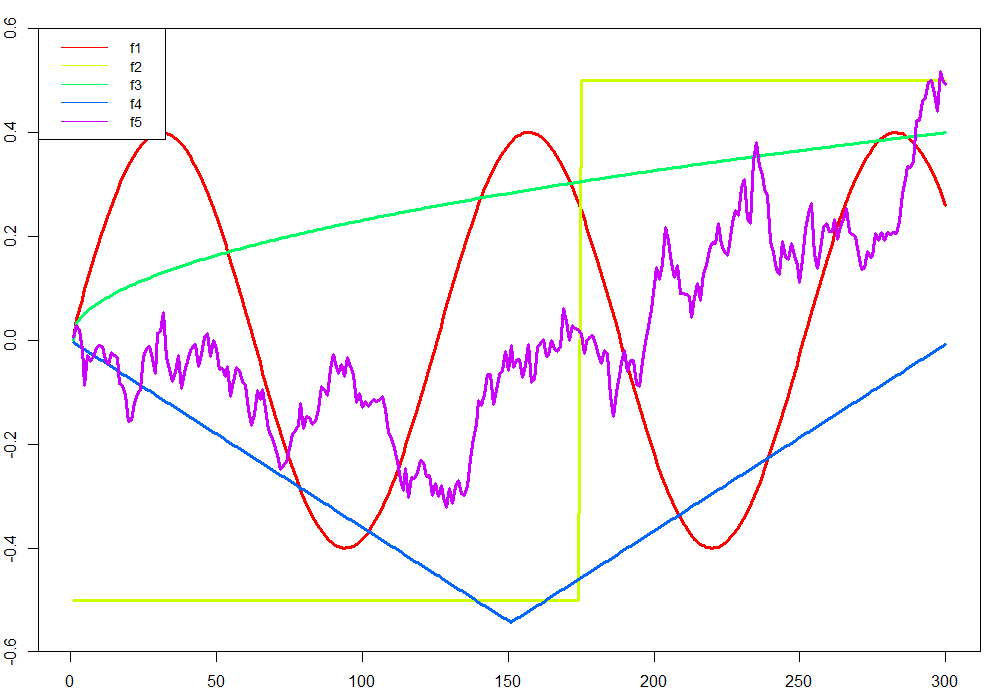
Figure 4: This graph displays the 5 paths out of which the true $\beta_{k,t}$’s will be constructed for simulations.

I consider three numbers of observations $T\in\{150,300,600\}$. Most of the attention will be dedicated to $T=300$ since it is roughly the number of US quarterly observations we will have 15 years from now. The size of the original regressor matrix $X$ is $K\in\{6,20,100\}$ and the first regressor in each is the first lag of $y$. Figure 4 display the 5 types of parameters path $f_{i}$ that will serve as basic material: cosine, quadratic trend, discrete break, a pure random walk and a linear trend with a break. $f_{1}$, $f_{2}$ and $f_{4}$ "fit" relatively well with the prior that coefficients evolve smoothly whereas $f_{3}$ and $f_{5}$ can pose more difficulties. In those latter situations, TVP models are expected to underperform. The design for simulations $S_{1}$, $S_{2}$, $S_{3}$ and $S_{4}$ can be summarized in a less cryptic fashion as

• $\beta_{k,t}$ follow the red line or is time invariant

• $\beta_{k,t}$ follow the yellow line, the negative of it or is time invariant

• $\beta_{k,t}$ is either the green line or the red one in equal proportions, otherwise time-invariant.

• $\beta_{k,t}$ is a random mixture (loadings are drawn from a normal distribution) from the red, purple and blue lines. Some coefficients are also time-invariant.

The considered proportions of TVPs within the $K$ parameters are $\nicefrac{{K^{*}}}{{K}}\in\{0.2,0.5,1\}$. Formally, we have

$$\beta_{k,t}^{S_{1}} =(-1)^{k}I(k<\nicefrac{{K^{*}}}{{K}})f_{1,t}+I(k>\nicefrac{{K^{*}}}{{K}})\beta_{k,0}$$

$$\beta_{k,t}^{S_{2}} =(-1)^{k}I(k<\nicefrac{{K^{*}}}{{K}})f_{2,t}+I(k>\nicefrac{{K^{*}}}{{K}})\beta_{k,0}$$

$$\beta_{k,t}^{S_{3}} =(-1)^{k}I(k<\nicefrac{{K^{*}}}{{2K}})f_{3,t}+(-1)^{k}I(\nicefrac{{K^{*}}}{{2K}}<k<\nicefrac{{K^{*}}}{{K}})f_{1,t}+I(k>\nicefrac{{K^{*}}}{{K}})\beta_{k,0}.$$

$$\beta_{k,t}^{S_{4}} =I(k<\nicefrac{{K^{*}}}{{K}})\sum_{j\in\{1,4,5\}}l_{j,k}f_{j,t}\enskip,\quad l_{j,t}\sim N(0,1).$$

The scale of coefficients is manually adjusted to prevent explosive behavior and/or overwhelmingly high $R^{2}$’s. The most important transformation in that regard is a min-max normalization on the coefficient of $y_{t-1}$ to prevent unit/explosive roots or simply persistence levels that would drive the true $R^{2}$ above its targeted range. Regarding the latter, I consider four different types of noise process. Three of them are homoscedastic and have a {Low, Medium, High} noise level. Those are calibrated so that $R^{2}$’s are around 0.8, 0.5 and 0.3 for low, medium and high respectively. The last two noise processes are SV, which is the predominant departure from the normality of $\epsilon_{t}$ in applied macroeconomics. For better comparison with time-invariant volatility cases, those are "manually" forced (by a min-max normalization) to oscillate between a predetermined minimum and maximum. The first SV process is constrained within the Low and Medium noise level bounds. For the second, it is Low and High, making the volatility spread much higher than in the first SV process case.

Four estimators are considered: the standard TVP-BVAR with SV, the two-step Ridge Regression (2SRR), the Group Lasso Ridge Regression (GLRR) and the Generalized Reduced Rank Ridge Regression (GRRRR). TVP-BVAR results are only obtained for $K=6$ for obvious computational reasons. Performance is assessed using the mean absolute error (MAE) with respect to the true path. I then take the mean across 100 simulations for each setup. To make this multidimensional notation more compact, let us define the permutation $\mathcal{J}=\{K,\nicefrac{{K^{*}}}{{K}},\sigma_{\epsilon},S_{i}\}$. I consider simulations $s=1,...,50$ for all $\mathcal{J}$’s. Formally, for model $m$ and setup $\mathcal{J}$, the reported performance metric is $\frac{1}{50}\sum_{s=1}^{50}MAE_{\mathcal{J}}^{s,m}$ where

$$MAE_{\mathcal{J}}^{s,m}=\frac{1}{K}\frac{1}{T}\sum_{k=1}^{K}\sum_{t=1}^{T}|\beta_{k,t}^{\mathcal{J},s}-\hat{\beta}_{k,t}^{\mathcal{J},s,m}|.$$ (19)

3.1 Results

The results for $T=300$ are in Tables 3, 4, 5 and 6. With these simulations, I am mostly interested in verifying two things. First, I want to verify that 2SRR’s performance is comparable to that of the BVAR for models’ size that can be handled by the latter. Second, I want to demonstrate that additional shrinkage can help under DGPs that more of less fit the prior of reduced-rank and/or sparsity. To make the investigation of these two points visually easier by looking at the tables, the lowest MAE out of BVAR/2SRR for each setup is in blue while that of the best one out of all algorithms is in bold.

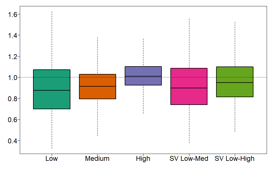
(a) By noise process

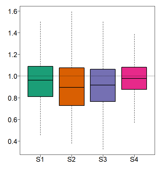
(b) By DGP

Figure 1: This figures summarizes tables 3, 4, 5 and 6 results comparing 2SRR and the BVAR when $K=6$ and $T=300$. The plotted quantity is the distribution of $\nicefrac{{MAE_{\mathcal{J}}^{s,2SRR}}}{{MAE_{\mathcal{J}}^{s,BVAR}}}$ for different subsets of interest.

Overall, results for 2SRR and the BVAR are very similar and their relative performance depends on the specific setup. These two models are interesting to compare because they share the same prior for TVPs (no additional shrinkage) but address evolving residuals volatility differently. Namely, the BVAR models SV directly within the MCMC procedure whereas 2SRR is a two-step GLS-like approach using a GARCH(1,1) model of the first step’s residuals. Figure 1 summarizes results of the 2SRR/BVAR comparison by reporting boxplots showcasing the distribution of relative MAEs (2SRR/BVAR) for different subsets. Overall, 2SRR does marginally better in almost all cases. A lower noise level seems to help its cause. It is plausible that cross-validating $\lambda$ as implemented by 2SRR plays a role (BVAR uses default values).

In Table 3, where the DGP is the rather friendly cosine-based TVPs, it is observed that the BVAR will usually outperform 2SRR by a thin margin when the level of noise is high. The reverse is observed for low noise environment and results are mixed for the medium one. Results for the SV cases will the subject of its own discussion later. For $K=6$, GLRR will marginally improve on 2SRR for most setups, especially those where 2SRR is already better than BVAR. In higher dimensions ($K=20$ or $K=100$), GLRR constantly improves on 2SRR (albeit minimally) whereas GRRRR can provide important gains (see the $\nicefrac{{K^{*}}}{{K}}=1$ block for instance) but is more vulnerable in the high noise environment.

In Table 4, where the DGP is the antagonistic structural break, 2SRR is clearly performing better than the BVAR, providing a smaller average MAE in 12 out of 15 cases for $K=6$. Still for the small dimensional case, it is observed that GLRR can further reduce the MAE — albeit by a very small amount — in many instances. The same is true for GRRRR when all parameters vary ($\nicefrac{{K^{*}}}{{K}}=1$). For GRRRR, this observation additionally extends to $K=20$, an environment where it is expected to thrive. Nonetheless, for setups where only a fraction of parameters vary, 2SRR and GLRR are the best alternatives for all $K$’s.

In Table 5, where the DGP is a mix of trending coefficients and cosine ones, Table 5 reports very similar results to that of Simulation 1. 2SRR is better than BVAR except in the high noise setups, where the latter has a minor advantage. GLRR often marginally improves upon 2SRR whereas GRRRR’s edge is more visible in low-noise and high-dimensional environments — factors being more precisely estimated with a large cross-section.

For the simulation in Table 6, a sophisticated mixture of TVP-friendly and -unfriendly parameters paths, BVAR does a better job than 2SRR for 8 out of 15 cases. The gains are, as before, quantitatively small. When 2SRR does better, gains are also negligible, suggesting that BVAR and 2SRR provide very similar results in this environment. When it comes to higher-dimensional setups ($K=20$ or $K=100$), GLRR emerges as the clear better option with (now familiar) marginal improvements with respect to 2SRR. This recurrent observation is potentially due to the iterative process producing a more precise $\hat{\Omega}_{u}$ when $\sigma_{u_{k}}^{2}$’s are heterogeneous whether sparsity is involved or not.

Table 1: Average Computational Time in Seconds

	$T=150$				$T=300$				$T=600$
	$K=6$	$K=20$	$K=100$		$K=6$	$K=20$	$K=100$		$K=6$	$K=20$	$K=100$
BVAR	219.3	–	–		513.7	–	–		1105.1	–	–
2SRR	0.3	0.9	2.7		1.0	3.1	12.4		4.8	14.1	69.5
GLRR	0.3	1.2	3.7		1.3	4.1	17.0		6.9	20.9	99.2
GRRRR	2.4	5.1	22.1		4.5	6.9	42.9		14.4	20.5	98.9

• Notes: The average is taken over DGPs’s, $\nicefrac{{K^{*}}}{{K}}=1$, noise processes, and all 100 runs. For all $\sim$RR models, this includes tuning cross-validating $\lambda$.

The results for $T=150$ and $T=600$ are in Tables 7, 8, 9, 10, 11, 12, 13 and 14. When $T$ is reduced from 300 to 150, the performance of 2SRR relative to that of BVAR remains largely unchanged: both report very similar results. When bumping $T$ to 600, overall performance of all estimators improves, but not by a gigantic leap. This is, of course, due to the fact that increasing $T$ also brings up the number of effective regressors. BVAR has a small edge on Simulation 1 in Table 11 whereas 2SRR wins marginally for the more complicated Simulation 4 (Table 14). What is most noticeable from those simulations with a larger $T$ is how much more frequently GLRR and especially GRRRR are preferred, especially in the medium- and high-dimensional cases. For instance, for the Cosine DGP ($S_{1}$) with $K\in\{20,100\}$, GRRRR almost always deliver the lowest MAE, and sometimes by good margins (e.g., $\{S_{1},\nicefrac{{K^{*}}}{{K}}=1,\sigma_{\epsilon}=\text{Low}\}$ for both $K$’s). Similar behavior is observed for $S_{3}$ in almost all cases of $K=20$. This noteworthy amelioration of GRRRR is intuitively attributable to factor loadings being more precisely estimated with a growing $T$. Thus, unlike 2SRR whose performance is largely invariant to $T$ by model design, algorithms incorporating more sophisticated shrinkage schemes may benefit from larger samples.

A pattern emerges across the four simulations: when SV is built in the DGP ($\sigma_{\epsilon,t}$ in tables), 2SRR either performs better or deliver roughly equivalent results to that of the BVAR. Indeed, with $T=300$, for 17 out of 24 setups with SV-infused DGPs, 2SRR supplants BVAR. The wedge is sometimes small ($\{S_{1},\nicefrac{{K^{*}}}{{K}}=0.2,\text{SV Low-Med}\}$,$\{S_{4},\nicefrac{{K^{*}}}{{K}}=1,\text{both SV}\}$), sometimes large ($\{S_{1},\nicefrac{{K^{*}}}{{K}}=1,\text{SV Low-High}\}$,$\{S_{2},\nicefrac{{K^{*}}}{{K}}=0.5,\text{both SV}\}$). However, it fair to say that small gaps between 2SRR and BVAR performances are the norm rather than the exception. Nonetheless, these results suggest that 2SRR is not merely a suboptimal approximation to the BVAR in the wake of computational adversity. It is a viable statistical alternative with the additional benefit of being easy to compute and to tune.

Speaking of computations, Table 1 reports how computational time varies in $K$ and $T$ on a cluster, and how 2SRR compares to a standard BVAR implementation. When $T$ is 300 and $K$ is 6, 2SRR takes one second while BVAR takes 513 seconds. When $T$ increases to 600, BVAR takes over 1 000 seconds whereas 2SRR takes less than 5. $T=300$ with $K=300$ can be seen as a typical high-dimensional case. It takes 13 seconds to compute (and tune) 2SRRR. When $T$ is reduced to 150, high-dimensional 2SRR runs in less than 3 seconds on average. Only when both $T$ and $K$ gets very large (by traditional macro data sets standards) do things become harder with 2SRR taking 69.5 seconds on average. By construction, GLRR takes marginally longer than 2SRR. Finally, by relying on an EM algorithm, GRRRR inevitably takes longer, yet remains highly manageable for very large models with many observations – taking a bit more than 100 seconds.

Table 2: Comparison in Higher Dimensions for Mixture DGP and $T=300$

		$K=20$							$K=50$
		2SRR		ShTVP-R		ShTVP-3G			2SRR		ShTVP-R		ShTVP-3G
$\mathbf{\nicefrac{{K^{*}}}{{K}}=0.2}$
$\sigma_{\epsilon}=\text{Low}$		0.067		0.074		0.063			0.103		0.121		0.101
$\sigma_{\epsilon}=\text{Medium}$		0.113		0.130		0.115			0.178		0. 198		0. 166
$\sigma_{\epsilon}=\text{High}$		0.233		0.239		0.202			0. 387		0. 348		0. 241
$\sigma_{\epsilon,t}=\text{SV Low-Med}$		0.087		0.095		0.081			0. 127		0. 148		0. 130
$\sigma_{\epsilon,t}=\text{SV Low-High}$		0.128		0.14		0.121			0. 216		0. 207		0. 169
$\mathbf{\nicefrac{{K^{*}}}{{K}}=0.5}$
$\sigma_{\epsilon}=\text{Low}$		0.088		0.085		0.081			0. 121		0. 132		0. 117
$\sigma_{\epsilon}=\text{Medium}$		0.130		0.139		0.130			0. 186		0. 205		0. 181
$\sigma_{\epsilon}=\text{High}$		0.239		0.245		0.207			0. 394		0. 353		0. 254
$\sigma_{\epsilon,t}=\text{SV Low-Med}$		0.102		0.105		0.095			0. 142		0. 156		0. 141
$\sigma_{\epsilon,t}=\text{SV Low-High}$		0.137		0.141		0.13			0. 220		0. 215		0. 183
$\mathbf{\nicefrac{{K^{*}}}{{K}}=1}$
$\sigma_{\epsilon}=\text{Low}$		0.111		0.104		0.109			0. 151		0. 151		0. 144
$\sigma_{\epsilon}=\text{Medium}$		0.151		0.155		0.155			0. 213		0. 222		0. 202
$\sigma_{\epsilon}=\text{High}$		0.268		0.258		0.230			0. 415		0. 364		0. 278
$\sigma_{\epsilon,t}=\text{SV Low-Med}$		0.127		0.125		0.125			0. 164		0. 173		0. 159
$\sigma_{\epsilon,t}=\text{SV Low-High}$		0.162		0.156		0.151			0. 229		0. 227		0. 200
Running Times
Seconds		5		70		70			13		360		362

• Notes: This table reports the average MAE of estimated $\beta_{t}$’s for various models. Seconds are from running such models on a 2020 M1 Macbook Air. MAE are averaged over 20 simulations.

Benchmarking in Higher Dimensions. In the years following the original draft of this paper, new Bayesian procedures have been proposed and packaged in statistical software. This allows for an easier evaluation of 2SRR in higher dimensions, both statistically and computationally. One such package is shrinkTVP from knaus2021shrinkage. It conveniently features C++ based computations, a very wide set of potential prior specifications, focus on single equation modeling, and features a data-driven way of choosing shrinkage intensity. Two default specifications are used, one with a ridge prior (ShTVP-R) on coefficients and another with the triple gamma prior (ShTVP-3G) of cadonna2020triple). The former is the closest relative to 2SRR within the suite of available configurations. The latter should perform well in the sparse TVP environments for which it has been designed. The high dimensional case of $K=100$ has been reduced to $K=50$ since it took shrinkTVP 38 minutes to estimate a single model in the original large $K$ case.

Results in Table 2 further establish the relevance of 2SRR for the estimation of models with many TVPs. Its statistical performance is mostly on par with ShTVP-R, with differences always being marginal in favor of one or another. ShTVP-3G can provide some less trivial improvements over both 2SRR andShTVP-R under a sparse DGP or in the hostile high noise and $K=50$ environment. Otherwise, it does not meaningfully outperform 2SRR. This is evidently the prior’s doing, and it is an empirical question as to which setup in Table 2 most closely resembles real data.

The Bayesian computations are manageable for $K=20$, and becomes rather burdensome for $K=50$ (about 10 minutes vs less than 15 seconds). Even at $K=20$, the fact that 2SRR gets similarly valid estimates in 5 seconds rather than in over a minute makes it more convenient in applied work where the trial and error of specifications (and sometimes even grid search of them) is widespread. It is apparent that for large models rolling/expanding window forecasting evaluations as in section 4 and large local projections as in 5, 2SRR remains the only practical game in town. Of course, full-blown Bayesian estimation directly provides many additional quantities that 2SRR does not procure readily, and its computational time could be brought down to a certain extent by cutting MCMC iterations. Nonetheless, the point is that, depending on the intended use, the ridge-based methods have non-trivial comparative advantages in many ways that are relevant for applied work.

4 Forecasting

In this section, I present results for a pseudo-out-of-sample forecasting experiment at the quarterly frequency using the dataset FRED-QD (mccracken2020fred). The latter is publicly available at the Federal Reserve of St-Louis’s web site and contains 248 US macroeconomic and financial aggregates observed from 1960Q1. The forecasting targets are real GDP, Unemployment Rate (UR), CPI Inflation (INF), 1-Year Treasury Constant Maturity Rate (IR) and the difference between 10-year Treasury Constant Maturity rate and Federal funds rate (SPREAD). These series are representative macroeconomic indicators of the US economy which is based on GCLSS2018’s exercise for many ML models, itself based on KLS2019 and a whole literature of extensive horse races in the spirit of SW1998comparison. The series transformations to induce stationarity for predictors are indicated in mccracken2020fred. For forecasting targets, GDP, CPI and UR are considered $I(1)$ and are first-differenced. For the first two, the natural logarithm is applied before differencing. IR and SPREAD are kept in "levels". Forecasting horizons are 1, 2, and 4 quarters. For variables in first differences (GDP, UR and CPI), average growth rates are targeted for horizons 2 and 4.

The pseudo-out-of-sample period starts in 2003Q1 and ends 2014Q4. I use expanding window estimation from 1961Q3. Models are estimated and tuned at each step. I use direct forecasts, meaning that $\hat{y}_{t+h}$ is obtained by fitting the model directly to $y_{t+h}$ rather than iterating one-step ahead forecasts. Following standard practice in the literature, I evaluate the quality of point forecasts using the root Mean Square Prediction Error (MSPE). For the out-of-sample (OOS) forecasted values at time $t$ of variable $v$ made $h$ steps ahead, I compute

$$RMSPE_{v,h,m}=\sqrt{\frac{1}{\#\text{OOS}}\sum_{t\in\text{OOS}}(y_{t}^{v}-\hat{y}_{t-h}^{v,h,m})^{2}}.$$

The standard dieboldmariano (DM) test procedure is used to compare the predictive accuracy of each model against the reference AR(2) model. $RMSPE$ is the most natural loss function given that all models are trained to minimize the squared loss in-sample.

Three types of TVPs will be implemented: 2SRR (section 2.4), GLRR (section 2.5.1), GRRRR (section 2.5.2). I consider augmenting four standard models with different methodologies proposed in this paper. The first will be an AR with 2 lags. The second is the well-known sw2002 ARDI (Autoregressive Diffusion Index) with 2 factors and 2 lags for both the dependent variable and the factors. The third is a VAR(5) with 2 lags and the system is composed of the 5 forecasted series. Finally, I consider as a fourth model a VAR(20) with 2 lags in the spirit of banbura2010large’s medium VAR. Thus, there is a total of $4\times 4=16$ models considered in the exercise. The BVAR used in section 3 is left out for computational reasons — models must be re-estimated every quarter for each target. Moreover, the focus of this section is rather single equation direct (as opposed to iterated) forecasting.

The first three constant coefficients models are estimated by OLS, which is standard practice. Since the constant parameters VAR(20) has 41 coefficients and around 200 observations, it is estimated with a ridge regression. Potential outliers are dealt with as in GCLSS2018 for Machine Learning models. If the forecasted values are outside of $[\boldsymbol{\bar{y}}+2*min(\boldsymbol{y}-\boldsymbol{\bar{y}}),\boldsymbol{\bar{y}}+2*max(\boldsymbol{y}-\boldsymbol{\bar{y}})]$, the forecast is discarded in favor of the constant parameters forecast.

4.1 Results

I report three sets of results. Table 15 corresponds exactly to what has been described beforehand. Table 16 gathers results where TVPs have been additionally shrunk to their constant parameters counterparts by means of model averaging with equal weights. The virtues of this Half & Half strategy are two-fold. First, k-fold CV can be over-optimistic for horizons $h$>1 because of imminent serial correlation. Second, k-fold CV ranks potential $\lambda$’s using the whole sample, whereas in the case of "forecasting", prediction always occurs at the boundary of the implicit kernel. In that region, the variance is mechanically higher and ensuing predictions could benefit from extra shrinkage. Shrinking to OLS in this crude and transparent fashion is a natural way to attempt getting even better forecasts. Finally, Table 17 reports results where k-fold CV has been replaced by Blocked k-fold CV (BCV) with blocks of 8 quarters as in, e.g., (MRF). This is a more principled strategy to curb the downward bias of $\lambda$ induced by serial dependence. Among other things, it does not rely on blending two models using intuitive but admittedly arbitrary weights.

Results with Basic CV and Half & Half. Overall, results are in line with evidence previously reported in the TVP literature: very limited improvements are observed for real activity variables (GDP, UR) whereas substantial gains are reported for INF and IR. For the latter, allowing for time variation in either AR or a compact factor model (ARDI) generate very competitive forecasts. For instance, ARDI-2SRR is the best model for IR with a reduction of 36% in RMPSE over the AR(2) benchmark which is strongly statistically significant. Still for IR, at horizon 2 quarters, iterating 2SRR to obtain GLRR generate sizable improvements for both AR and ARDIs. VAR(20) is largely inferior to alternatives in any of its forms. Two exceptions are IR forecasts at a one-year horizon where combining VAR(20) with GRRRR yields the best forecast by a wide margin with improvement of 19% in RMSPE. VAR(20)-GRRRR also provide a very competitive forecast for IR at an horizon of one quarter. Finally, at horizon 1 quarter, any form of time variation (2SRR, GLRR, GRRRR) at least increases SPREAD’s forecasting accuracy for for all models but the VAR(20). Precisely, it is a 16% reduction in RMSPE for AR, about 5% for ARDI and up to 14% in the VAR(5) case. For the latter, its combination with 2SRR provides the best forecast with a statistically significant improvement of 18% with respect to the AR(2) benchmark.

A notable absence from the relatively cheerful discussion above is inflation, which is the first (or second) variable one would think should benefit from time variation. It is clear that, in Table 15, any AR at horizon 1 profits rather timidly from it. A similar finding for Half & Half is reported in Table 16. What differs, however, are longer horizons results for INF. Indeed, mixing in additional shrinkage to OLS strongly helps results for those targets: every form of time variation now improves performance by a good margin. For instance, any time-varying ARs improves upon the constant benchmark by around 15%. It is now widely documented that inflation prior to the Pandemic was better predicted by past values of itself and not much else – besides maybe for recessionary episodes (KLS2019). Results of Table 16 comfortably stand within this paradigm except for the noticeable efforts from GLRR versions of both ARDI and VAR(20). While those are the best models, they are closely matched in performance by their AR counterparts. Nevertheless, it is noteworthy that this surge in performance mostly occurs for their sparse TVP versions, suggesting time variation is likely crucial for more sophisticated inflation forecasts not to be off the charts. Finally, additional shrinkage marginally improves GDP forecasting at the two longer horizons, with the Half & Half ARDI-GLRR providing the best forecasts.

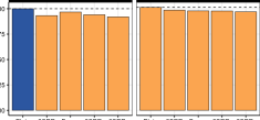
(a) Inflation ($h=1$)

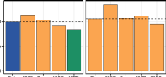
(b) Inflation ($h=2$)

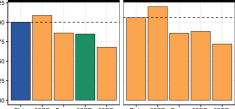
(c) Inflation ($h=4$)

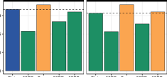
(d) Interest Rate ($h=1$)

Figure 2: A subset of $RMSPE_{v,h,m}/RMSPE_{v,h,\text{Plain AR(2)}}$’s (from Tables 15 and 16) for forecasting targets usually associated with the need for time variation. Blue is the benchmark AR with constant coefficients. Dark green means that the competing forecast rejects the null of a Diebold-Mariano test at least at the 10% level (with respect to the benchmark). Orange means that it does not. "Bayes" corresponds to results from Bayesian approach, precisely the Triple Gamma prior model as available from the ShrinkTVP package.

Blocked CV and an Overall Assessment. Coming to Table 17, we see that switching from CV to Blocked CV offers comprehensive gains. Large losses to constant parameters models for real activity variables have been substantially mitigated and sometimes turned into marginal gains (for instance, ARDI-2SRR, unemployment at $h=1$). Overall, at $h=1$, gains from BCV are located where those of Half & Half are, which is intuitive. Things are more heterogeneous at longer horizons. The most notable amelioration is that of inflation, where 2SRR (and variants) now brings important gains across the board. BCV being such a game changer for INF requires little creativity in explaining it. Inflation is highly persistent for a great part of the training sample, which may have misled plain CV in choosing too low of a $\lambda$. Note that, interestingly, BCV does not fare as well for IR as other strategies did. One way to rationalize this is that "arbitrarily" opting for a lower $\lambda$ through non-blocked CV may have helped with the massive and rapid structural change that occurred when the zero-lower bound was hit in the test sample. We can posit that this event with no historical precedent likely induced desirable time variation in $\lambda$ itself. Thus, for a panoply of unforeseen reasons, it is absolutely possible that $\lambda^{\text{CV}}$ is closer to the ex-post optimal $\lambda$ than $\lambda^{\text{BCV}}$, even if BCV dominates CV in principle for dependent data.

To a large extent, forecasting results suggest that the three main algorithms presented in section 2 can procure important gains for forecasting targets that are frequently associated with the need for time variation. This subset is put on the spotlight by Figure 2. The gains for IR at $h=1$ and INF at the two quarters and one-year horizon are particularly visible. For those kinds of targets, it is observed that any form of time-variation will usually ameliorate the constant parameters benchmark, especially in the Half & Half and BCV cases. We also see that those perform comparably well or better than a state-of-the-art Bayesian approach, precisely the Triple Gamma prior model from cadonna2020triple using default hyperparameters. Of course, both the ridge and Bayesian approach have distinct merits, but it is interesting to note that ShrinkTVP marginal advantage in simulations seems to be reversed in this real data application.

5 Time-Varying Effects of Monetary Policy in Canada

VARs do not have a monopoly on the proliferation of parameters. jorda2005 local projections’ – by running a separate regression for each horizon – are also densely parametrized. For that reason, constructing a large LP-based time-varying IRF via a MCMC procedure would either be burdensome or unfeasible. In this section, I demonstrate how 2SRR is up to the task by estimating LPs chronicling the evolving effects of Canadian monetary policy over recent decades.

The use of 2SRR for estimation of LPs constitutes a very useful methodological development given how popular local projections have become over recent years. Particularly, it is appealing for researchers to identify shocks in a narrative fashion (for instance, à la romerromer2004) and then use those in local projections to obtain their dynamic effects on the economy. A next step is to wonder about the stability of the estimated relationship. In that line of thought, popular works include AG2012 and RZ2018 for the study of state-dependent fiscal multipliers. To focus on long-run structural change rather than switching behavior, random walk TVPs are a natural choice and 2SRR, a convenient estimation approach.

In this application, I study the changing effects of monetary policy (MP) in Canada using the recently developed MP shocks series of champagnesekkel2018. The small open economy went through important structural change over the last 30–40 years. Most importantly, from a monetary policy standpoint, it became increasingly open (especially following NAFTA) and an inflation targeting regime (IT) was implemented in 1991 – a specific and publicly known date. Both are credible sources of structural change in the transmission of monetary policy. champagnesekkel2018 estimate a parsimonious VARs (4 variables) over two non-overlapping subsamples to check visually whether a break occurred in 1992 following the onset of IT. The reported evidence for a break is rather weak with GDP’s response increasing slightly while that of inflation decreasing marginally. While the sample-splitting approach has many merits such as transparency and simplicity, there is arguably a lot it can miss. I go further by modeling the full evolution of their LP-based IRFs.

I use the same monthly Canada data set as in champagnesekkel2018 and the analysis spans from 1976 to 2015. The target variables are unemployment, CPI Inflation and GDP. Their original specification includes 48 lags of the narrative monetary policy (MP) shock series which is constructed in the spirit of romerromer2004 and carefully adapted to the Canadian context. Furthermore, their regression comprises 4 lags for the controls which are first differences of the log GDP, log inflation and log commodity prices. To certify that time-variation will not be found as a result of omitted variables, I increase the lag order from 4 to 6 months and augment the model with the USD/CAD exchange rate, exports, imports and CPI excluding Mortgage Interest Cost (MIC). In terms of TVP accounting, $\boldsymbol{X}$ contains 97 regressors (including the constant) and $\boldsymbol{Y}$ is $48$. Thus, a single TV-LP is assembled from a staggering total of $97\times 48=4\,656$ TVPs.

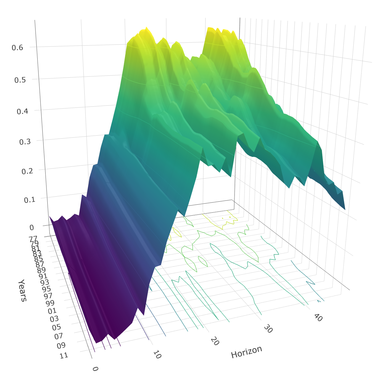
(a) Unemployment

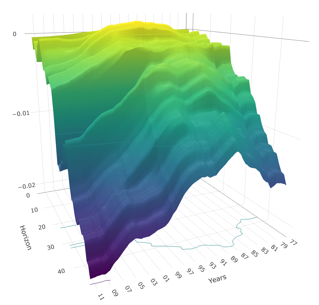
(b) CPI Inflation

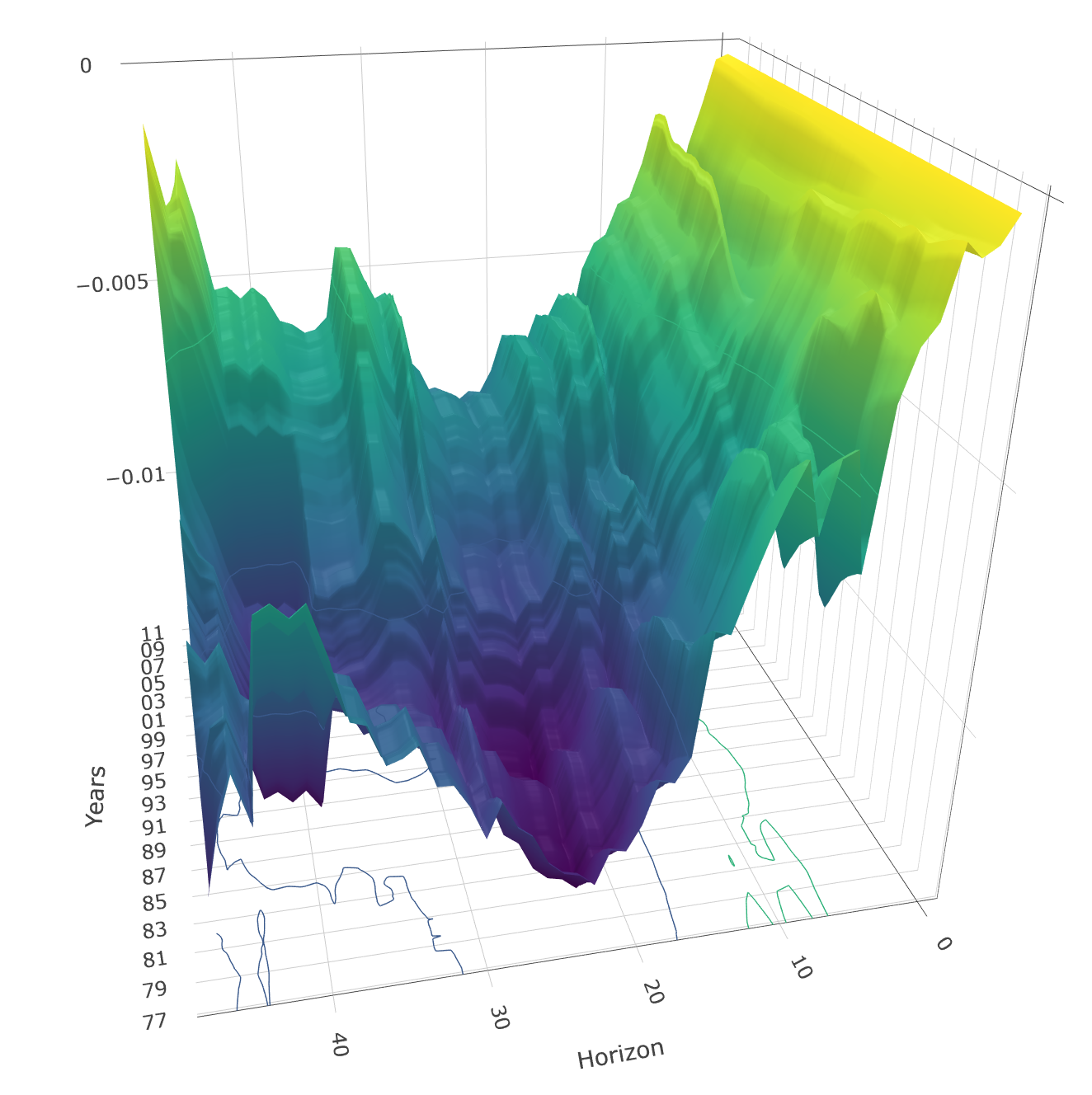
(c) GDP

Figure 3: Cumulative Time-Varying Effect of Monetary Policy Shocks. Rotations of 3D plots are hand-picked to highlight most salient features of each time-varying IRF. Interactive plots where the reader can manually explore different rotations are available here.

Figure 3 proposes clear answers to the evolving effect of monetary policy on the economy. Generally, short- and medium-run effects ($h<24$ months) have been much more stable than longer-run ones. This is especially true of unemployment which exhibits a strikingly homogeneous response (through time) for the first year and half after the shock. GDP’s response follows a similar predicament, but was marginally steeper before the 2000s. When it comes to inflation, its usual long response lag has mildly shortened up in the 2000s. At a horizon of 24 months, the effect of a positive one standard deviation shock was -0.3% from 1976 to the late 1990s, then slowly increased (in absolute terms) to nearly double at -0.6%. Overall, results for horizons up to 18 months suggest that the ability of the central bank to (relatively) rapidly impact inflation has increased, while that of GDP has decreased and that of unemployment remained stable.

Given the long lags of monetary policy, most of the relevant action from an economic standpoint is also where most time variation is found: from 1.5 to 4 years after the shock. Regarding GDP and unemployment, the cumulative long-run effects of MP shocks have substantially shrunk over the sample period. For unemployment, the decrease from a 0.6 to 0.4 unemployment percentage points effect mostly occurred throughout the 1980s, and stabilized at 0.4 thereafter. For GDP, both its peak effect (at around $h=24$ months) and the long-run one shrunk from the 1990s onward. Both quantities are about twice smaller around 2011 than they were in 1991. The long-run cumulative effect on inflation follows a distinctively different route: it has considerably expanded starting from the late 1980s. The overall effect on CPI, four years after impact, doubled from -1% in 1987 to -2% in 2011.

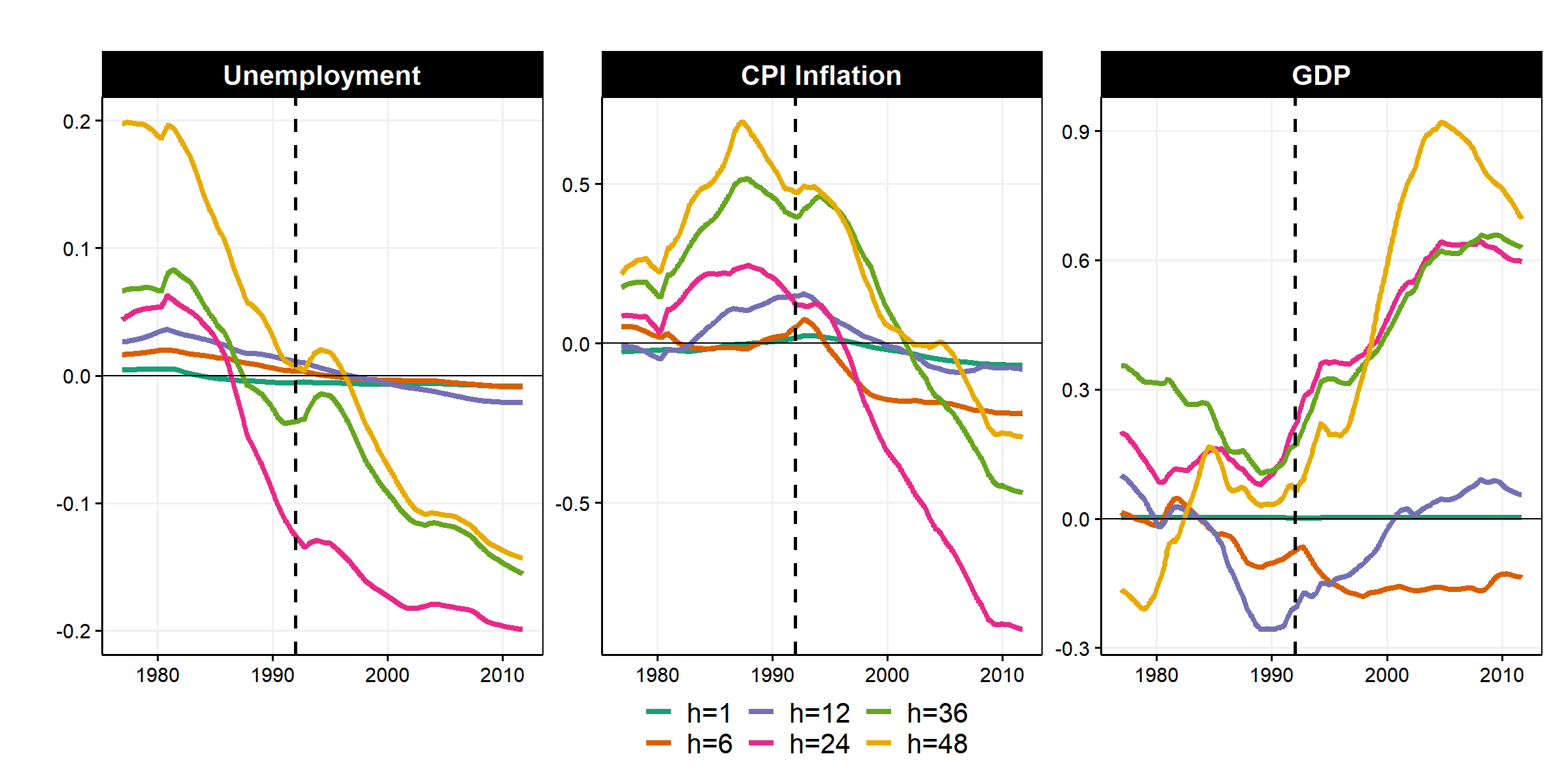
Figure 6: $\beta_{t}^{2SRR}-\beta^{OLS}$ for the cumulative effect of MP shocks on variables of interest. Note that for better visibility, GDP and CPI Inflation units are now percentages. Dashed black line is the onset of inflation targeting.

An important question is what happens to $\beta_{t}$ around 1992, after the onset of IT. Figure 6 (in the appendix) reports $\beta_{t}^{\text{2SRR}}-\beta^{\text{OLS}}$ for the dynamic effect of MP shocks on the three variables. It is found that the response of inflation (in absolute terms) is much larger at the end of the sample than what constant coefficients would suggest. This is especially true at the 24 months horizon. It is quite clear that, for all horizons, the effect of MP shocks on inflation starts increasing in the years following the implementation of IT. The vanishing effect on GDP starting from the 1990s could be consistent with an increased openness of the economy limiting the central bank’s grip on economic activity. The story is, however, different for unemployment. The downward trend in MP shocks’ impact seems to have started at least since the 1970s and slowed down in recent years. More generally, it is interesting to note that those results are consistent with some flattening of the unemployment- or GDP-based Phillips’ curve, at least, which was a well-established observation, at least, before the COVID-19 pandemic blanchard2015inflation; del2020s. The shrinking responses of GDP and unemployment leave room for expectations to act as the main channel through which MP shocks (eventually) impact the price level.

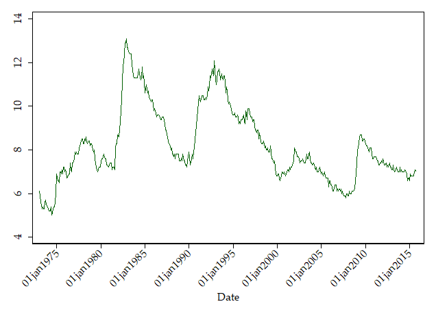
(a) Unemployment Rate

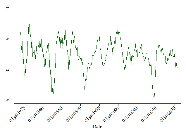
(b) Month over Month GDP growth

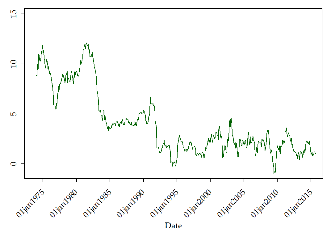
(c) Month over Month Inflation Rate

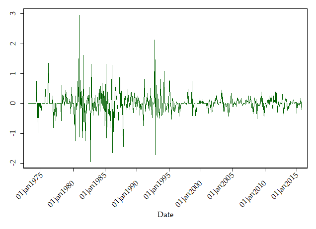
(d) Monetary Policy Shocks

Figure 5: Four Main Canadian Time series

The evidence on the effects of IT is mixed. ramey2016hb and barakchian2013monetary obtain counterintuitive results (a price puzzle and MP tightening increases GDP) for post-1988 US data. cloyne2016macroeconomic and champagnesekkel2018 report less economics-contorting findings for the UK and Canada: GDP response increases marginally after IT and that of inflation shrinks. 2SRR-LPs signs and magnitudes are consistent with those reported in champagnesekkel2018. Moreover, Figure 6 does not suggest the occurrence of a structural break in 1992, which is in line with most of the international evidence on IT implementation. Nonetheless, at least for GDP and inflation, 2SRR-LPs’ results point to a drastic change in coefficients’ trending behavior, a subtle phenomenon which effectively stays under the radar of simpler approaches. Particularly, when looking at various $\beta_{t,h}^{\text{2SRR}}-\beta_{h}^{\text{OLS}}$ for inflation in Figure 6, it is self-evident why mere splitting of the sample would not find any significant change. Additionally, the staircase-like trajectory of Canadian inflation in the 1980s (Figure 5(c)) is visually supportive of a TVP approach for the intercept, and cast strong doubts about any approach assuming only two regimes.

Unlike most of their predecessors, results presented in this section rely on an approach that is jointly flexible (i) in the specification of dynamics by using LPs, (ii) in the information set by allowing for many controls and (iii) in the time variation by fully modeling $\beta_{t}$’s path. The 2SRR-based LPs display that while the cumulative effect of MP shocks became more muted for real activity variables, it has increased for inflation. This suggests that stabilizing Canadian inflation is less costly (in terms of unemployment/GDP variability) within the IT framework.

6 Conclusion

I provide a new framework to estimate TVP models with potentially evolving volatility of shocks. It is conceptually enlightening and computationally very fast. Moreover, seeing such models as ridge regressions suggest a simple way to tune the amount of time variation, a neuralgic quantity. The approach is easily extendable to have additional shrinkage schemes like sparse TVPs or reduced-rank restrictions. The proposed variants of the methodology are very competitive against the standard Bayesian TVP-VAR in simulations. Furthermore, they improve forecasts against standard forecasting benchmarks for variables usually associated with the need for time variation (US inflation and interest rates). Finally, I apply the tool to estimate time-varying IRFs via local projections. The large specification necessary to characterize adequately the evolution of monetary policy in Canada rendered this application likely unfeasible without the newly developed tools. I report that monetary policy shocks long-run impact on the price level increased substantially starting from the early 1990s (onset of inflation targeting), whereas the effects on real activity became milder.

Appendix A Appendix

A.1 Details of GLRR

To begin with, the penalty part of (11) in summation notation is

$$\sum_{k=1}^{K}\frac{1}{\sigma_{u_{k}}^{2}}{\sum_{t=1}^{T}}u_{k,t}^{2}+\xi{\sum_{k=1}^{K}}|{\sigma_{u_{k}}}|.$$

The E-step of the procedure provides a formula for $\sigma_{u_{j}}$ in terms of $u$’s. Plugging it in gives

$$\sum_{k=1}^{K}\frac{1}{\sigma_{u_{k}}^{2}}{\sum_{t=1}^{T}}u_{k,t}^{2}+\xi{\sum_{k=1}^{K}}({\sum_{t=1}^{T}}u_{k,t}^{2})^{\frac{1}{2}}.$$

which is just a Group Lasso penalty with an additional Ridge penalty for each individual coefficients. Hence, classifying parameters into TVP or non-TVP categories is equivalent to group selection of regressors where each $k$ of the $K$ groups is defined as $\{Z_{t,k,\tau}\}_{\tau=1}^{\tau=T}$. If we want a parameter to be constant, we trivially have to drop block-wise its respective basis expansion regressors and only keep $\beta_{0,k}$ in the model.

This penalty can be obtained by iterating what we already have. grandvalet1998 shows that the Lasso solution can be obtained by iterative Adaptive Ridge. frommletnuel2016 and liuli2014 extend his results to obtain $l_{0}$ regularization without the computational burden associated with this type of regularization. frommletnuel2016 also argue in favor of a slightly modified version of grandvalet1998’s algorithm which I first review before turning to the final GLRR problem.

To implement Lasso by Adaptive Ridge, we have at iteration $i$,

$$\boldsymbol{b}_{i}=\arg\min_{\boldsymbol{b}}{\sum_{t=1}^{T}}\left(y_{t}-X_{t}\boldsymbol{b}\right)^{2}+\lambda{\sum_{=1}^{J}}w_{j}{b}_{j}^{2}$$

$$w_{i+1,j}=\frac{1}{(b_{i,j}+\delta)^{2}}$$

where $\delta>0$ is small value for numerical stability and we set $w_{j,0}=1\quad\forall j$. To get some intuition on why this works, it is worth looking at the penalty part of the problem in the final algorithm step:

$$\lambda{\sum_{j=1}^{J}}\frac{{b}_{j}^{2}}{|\hat{b}_{j}|+\delta}\approx\lambda{\sum_{j=1}^{J}}|{{b}_{j}}|.$$

liuli2014 show that this qualifies as a proper EM algorithm (each step improves the likelihood). Thus, we can expect it to inherit traditional convergence properties.

A.1.1 Building Iterative Weights for GLRR

The above methodology can be adapted for a case which is substantially more complicated. The complications are twofold. First, we are doing Group Lasso rather than plain Lasso. Second, the individual ridge penalty must be maintained on top of the Group Lasso penalty. I devise a simple algorithm that will split the original Ridge penalty into two parts, one that we will keep as is and one that will be iterated. The first is the 2SRR part and the second implements Group-Lasso.

Let us first focus on the Group penalty and display why iterating the Ridge solution with updating weights converges to be equivalent to Group Lasso. In the last step of the algorithm, we have

$$\xi{\sum_{k=1}^{K}}\frac{1}{\hat{\sigma}_{u_{k}}}{\sum_{t=1}^{T}}{u}_{k,t}^{2}\approx\xi{\sum_{k=1}^{K}}({\sum_{t=1}^{T}}{u}_{k,t}^{2})^{\frac{1}{2}}$$

where $\hat{\sigma}_{u_{k}}=({\sum_{t=1}^{T}}{u}_{k,t}^{2})^{\frac{1}{2}}$. The two penalties must be combined in a single penalizing weight that enters the closed-form solution. I split the original penalty into two parts, one that will remain as such and one that will be iterated to generate group selection. A useful observation is the following. For a given iteration $i$,

$$\lambda\sum_{k=1}^{K}\frac{1}{\sigma_{u_{k}}^{2}}{\sum_{t=1}^{T}}{u}_{k,t}^{2}+\xi{\sum_{k=1}^{K}}\frac{1}{\sigma_{u_{k}}^{(i)}}{\sum_{t=1}^{T}}{u}_{k,t}^{2}$$

can be re-arranged as

$$\sum_{k=1}^{K}\left[\frac{\lambda}{\sigma_{u_{k}}^{2}}+\frac{\xi}{{\sigma_{u_{k}}^{(i)}}}\right]{\sum_{t=1}^{T}}{u}_{k,t}^{2}.$$

To make this more illuminating, define $\alpha=\frac{\lambda}{\lambda+\xi}$ and $\tilde{\lambda}=(\lambda+\xi)$. We now have

$$\tilde{\lambda}\sum_{k=1}^{K}\left[\alpha\frac{1}{\sigma_{u_{k}}^{2}}+(1-\alpha)\frac{1}{\sigma_{u_{k}}^{(i)}}\right]{\sum_{t=1}^{T}}{u}_{k,t}^{2}.$$

where $\alpha\in(0,1)$ is a tuning parameter controlling how the original ridge penalty is split between smoothness and group-wise sparsity. It is now easy to plug this into the closed-form formula: stack $\lambda_{u_{k}}^{(i)}=\tilde{\lambda}\left[\alpha\frac{1}{\sigma_{u_{k}}^{2}}+(1-\alpha)\frac{1}{\sigma_{u_{k}}^{(i-1)}}\right]$ on the diagonal of $\Omega_{u_{i}}^{-1}$ at iteration $i$ in 2.4. The reader is now referred to the main text (section 2.5.1) for the benchmark algorithm that uses these derivations to implement GLRR.

A.1.2 Credible regions

Those can obtained from

$$V_{\boldsymbol{\beta}}=\boldsymbol{C_{*}}(\boldsymbol{Z_{*}}^{\prime}\Omega^{-1}_{\epsilon}\boldsymbol{Z_{*}}+\boldsymbol{\Omega}_{\theta_{*}}^{-1})^{-1}\boldsymbol{C_{*}}^{\prime}$$

where the $C_{*}$, $\boldsymbol{Z}_{*}$ and $\Omega_{\theta_{*}}$ are the part of the corresponding matrices left after leaving out the basis expansion parts that correspond to the selected constant parameters. The $*$ versions should be much smaller than the original one especially in a high-dimensional model. These bands take the model selection event as given.

A.2 Multivariate Extension to GRRRR

Dense TVPs as proposed (among others) by stevanovic2016common implement a factor structure for parameters of a whole VAR system rather than a single equation. If time-variation is indeed similar for all equations, we can decrease estimation variance significantly by pooling all parameters of the system in a single factor model. First, the factors are better estimated as the number of series increase. Second, the estimated factors are less prone to overfit because they now target $M$ series rather than a single one. The likely case where $r$ is smaller than $M$ (and $P$ not incredibly big) yields a models that will have more observations than parameters, in contrast to everything so far considered in this paper. I briefly describe how to modify Algorithm 3 to obtain Multivariate GRRRR (MV-GRRRR) estimates.

Starting values for the algorithm below can be obtained from the multivariate RR of section (2.4.4). This is done by first re-arranging elements of $\boldsymbol{\hat{\Theta}}$ into $\mathcal{U}=[\boldsymbol{U}_{1}\quad\dots\quad\boldsymbol{U}_{M}]$ and then running PCA on $\mathcal{U}$. Then, the MV-GRRRR solution can be obtained by alternating the following steps.

1. Given $\Lambda$, we can solve

   $$\min_{\boldsymbol{f},b_{0}}\left(vec(\boldsymbol{Y})-(I_{M}\otimes\boldsymbol{X})b_{0}-\boldsymbol{Z_{M}}^{\Lambda}\boldsymbol{f}\right)^{\prime}\Omega_{\epsilon_{M}}^{-1}\left(vec(\boldsymbol{Y})-(I_{M}\otimes\boldsymbol{X})b_{0}-\boldsymbol{Z_{M}}^{\Lambda}\boldsymbol{f}\right)+\boldsymbol{f^{\prime}f}$$ (A.1)

   where $\boldsymbol{Z_{M}}^{\Lambda}$ stacks row-wise all the $\boldsymbol{Z}(I_{T}\otimes\Lambda_{m})$ from $m=1$ to $m=M$. That is, we have the $TM\times Tr$ matrix

   $$\boldsymbol{Z_{M}}^{\Lambda}=\begin{bmatrix}\boldsymbol{Z}(I_{T}\otimes\Lambda_{1})\\ \boldsymbol{Z}(I_{T}\otimes\Lambda_{2})\\ \vdots\\ \boldsymbol{Z}(I_{T}\otimes\Lambda_{M})\end{bmatrix}$$

   as the regressor matrix. $\Lambda_{m}$ is a sub-matrix of $\Lambda$ that contains the loadings for parameters of equation $m$. Also, $b_{0}=vec(B_{0})$ where $B_{0}$ is the matrix that corresponds to the multivariate equivalent of $\beta_{0}$. Unlike a standard multivariate model like a VAR, here, we cannot estimate each equation separately because the $\boldsymbol{f}$ is common across equations.

2. The loadings updating step is

   $$\min_{l,b_{0}}\left(vec(\boldsymbol{Y})-(I_{M}\otimes\boldsymbol{X})b_{0}-\boldsymbol{Z^{F}_{M}}l\right)^{\prime}\Omega_{\epsilon_{M}}^{-1}\left(vec(\boldsymbol{Y})-(I_{M}\otimes\boldsymbol{X})b_{0}-\boldsymbol{Z^{F}_{M}}l\right)+\xi\|l\|_{1}$$ (A.2)

   where $\boldsymbol{Z^{F}_{M}}=(I_{M}\otimes\boldsymbol{Z}(\boldsymbol{F^{\prime}}\otimes I_{K}))$. This is just a Lasso regression. The Kronecker structure allows for these Lasso regressions to be ran separately.

As in bai2017principal for the estimation of regularized factor models, there is orthogonalization step needed between each of these steps to guarantee identification.

Note that if $MT>rT+MK$, which is somewhat likely, we have more observations than parameters in step 1. This means standard Ridge regularization is not necessary for the inversion of covariance matrix of regressors. Nonetheless, the ridge smoothness prior will still prove useful but can be applied in a much less aggressive way.

An interesting connection occurs in the MV-GRRRR case: the time-varying parameter model with a factor structure in parameters can also be seen as a dynamic factor model with deterministically time-varying loadings. By the latter, I mean that loadings change through time because they are interacted with a known set of (random) variables $X_{t}$. This is a more general version of kelly2017ipca Instrumented PCA used to estimate a typical asset-pricing factor model. Formally, this means that the factor TVP model

$$Y_{t}=X_{t}\Lambda F_{t}+\epsilon_{t},\quad\quad{F_{t}}={F_{t-1}}+{u}_{t}$$

can be rewritten as

$$Y_{t}=\Lambda_{t}F_{t}+\epsilon_{t},\quad\quad{F_{t}}={F_{t-1}}+{u}_{t},\quad\quad\Lambda_{t}=X_{t}\Lambda$$ (A.3)

which is the so-called Instrumented PCA estimator if we drop the law of motion for $F_{t}$. An important additional distinction is that kelly2017ipca consider cases where the number of instruments is smaller than the size of the cross-section. Here, with the instruments being $X_{t}$, there is by construction more instruments than the size of the cross-section. Nevertheless, the analogy to the factor model is conceptually useful and can point to further improvements of TVP models inspired by advances in empirical asset pricing research.

A.3 Simple GRRRR Example with $r=1$

While Kronecker product operations may seem obscure, they are the generalization of something that much more intuitive: the special case of one factor model ($r=1$). I present here the simpler model when parameters vary according to a single latent source of time-variation. For convenience, I drop evolving volatility and use summation notation. The problem reduces to

$$\min_{l,f,\beta_{0}}\sum_{t=1}^{T}\left(y_{t}-X_{t}\beta_{0}-\sum_{k=1}^{K}l_{k}f_{t}X_{k}\right)^{2}+\sum_{t=1}^{T}f_{t}^{2}+\xi\sum_{k=1}^{K}|l_{k}|$$ (A.4)

which can trivially rewritten as

$$\min_{l,f,\beta_{0}}\sum_{t=1}^{T}\left(y_{t}-X_{t}\beta_{0}-f_{t}\sum_{k=1}^{K}l_{k}X_{k,t}\right)^{2}+\sum_{t=1}^{T}f_{t}^{2}+\xi\sum_{k=1}^{K}|l_{k}|.$$ (A.5)

and this model can be estimated by splitting it two problems. The two steps are

1. Given the $l$ vector, we run the TVP regression

   $$\min_{f,\beta_{0}}\sum_{t=1}^{T}\left(y_{t}-X_{t}\beta_{0}-\bar{X}_{t}f_{t}\right)^{2}+\sum_{t=1}^{T}f_{t}^{2}.$$

   where $\bar{X}_{t}\equiv\sum_{k=1}^{K}l_{k}X_{k,t}$. Hence, the new regressors are just a linear combination of original regressors.

2. Given $f$, the second step is the Lasso regression (or OLS/Ridge if we prefer)

   $$\min_{l,\beta_{0}}\sum_{t=1}^{T}\left(y_{t}-X_{t}\beta_{0}-\sum_{k=1}^{K}l_{k}{X^{f}}_{k,t}\right)^{2}+\xi\sum_{k=1}^{K}|l_{k}|.$$

   where the $K$ new regressors are ${X^{f}}_{k,t}\equiv f_{t}X_{k,t}$.

A.4 Tables

Table 3: Results for Simulation 1 (Cosine) and $T=300$

	$K=6$					$K=20$					$K=100$
	BVAR	2SRR	GLRR	GRRRR		BVAR	2SRR	GLRR	GRRRR		BVAR	2SRR	GLRR	GRRRR
$\mathbf{\nicefrac{{K^{*}}}{{K}}=0.2}$
$\sigma_{\epsilon}=\text{Low}$	0.128	0.110	0.097	0.136		-	0.115	0.095	0.114		-	0.163	0.160	0.200
$\sigma_{\epsilon}=\text{Medium}$	0.159	0.165	0.163	0.193		-	0.165	0.161	0.169		-	0.197	0.192	0.314
$\sigma_{\epsilon}=\text{High}$	0.228	0.245	0.244	0.271		-	0.262	0.262	0.269		-	0.320	0.316	0.580
$\sigma_{\epsilon,t}=\text{SV Low-Med}$	0.129	0.121	0.110	0.145		-	0.131	0.120	0.132		-	0.168	0.166	0.242
$\sigma_{\epsilon,t}=\text{SV Low-High}$	0.143	0.151	0.152	0.174		-	0.159	0.158	0.175		-	0.189	0.189	0.293
$\mathbf{\nicefrac{{K^{*}}}{{K}}=0.5}$
$\sigma_{\epsilon}=\text{Low}$	0.169	0.130	0.120	0.144		-	0.150	0.135	0.129		-	0.256	0.256	0.263
$\sigma_{\epsilon}=\text{Medium}$	0.224	0.207	0.206	0.247		-	0.227	0.224	0.221		-	0.283	0.278	0.395
$\sigma_{\epsilon}=\text{High}$	0.274	0.291	0.292	0.330		-	0.314	0.311	0.316		-	0.371	0.365	0.700
$\sigma_{\epsilon,t}=\text{SV Low-Med}$	0.186	0.147	0.138	0.184		-	0.171	0.162	0.158		-	0.259	0.260	0.303
$\sigma_{\epsilon,t}=\text{SV Low-High}$	0.211	0.189	0.189	0.229		-	0.216	0.214	0.225		-	0.273	0.274	0.361
$\mathbf{\nicefrac{{K^{*}}}{{K}}=1}$
$\sigma_{\epsilon}=\text{Low}$	0.134	0.149	0.152	0.157		-	0.185	0.191	0.141		-	0.367	0.370	0.284
$\sigma_{\epsilon}=\text{Medium}$	0.302	0.242	0.247	0.282		-	0.278	0.289	0.252		-	0.389	0.388	0.467
$\sigma_{\epsilon}=\text{High}$	0.337	0.355	0.360	0.376		-	0.388	0.389	0.391		-	0.454	0.451	0.766
$\sigma_{\epsilon,t}=\text{SV Low-Med}$	0.171	0.168	0.172	0.180		-	0.208	0.215	0.156		-	0.380	0.381	0.351
$\sigma_{\epsilon,t}=\text{SV Low-High}$	0.262	0.222	0.232	0.268		-	0.262	0.274	0.261		-	0.383	0.382	0.368

• Notes: This table reports the average MAE of estimated $\beta_{t}$’s for various models. The number in bold is the lowest MAE of all models for a given setup. The number in blue is the lowest MAE between BVAR and 2SRR for a given setup.

Table 4: Results for Simulation 2 (Break) and $T=300$

	$K=6$					$K=20$					$K=100$
	BVAR	2SRR	GLRR	GRRRR		BVAR	2SRR	GLRR	GRRRR		BVAR	2SRR	GLRR	GRRRR
$\mathbf{\nicefrac{{K^{*}}}{{K}}=0.2}$
$\sigma_{\epsilon}=\text{Low}$	0.154	0.113	0.098	0.146		-	0.149	0.141	0.191		-	0.331	0.337	0.487
$\sigma_{\epsilon}=\text{Medium}$	0.216	0.176	0.165	0.296		-	0.249	0.256	0.294		-	0.587	0.578	1.165
$\sigma_{\epsilon}=\text{High}$	0.295	0.292	0.296	0.412		-	0.473	0.480	0.498		-	1.267	1.236	2.484
$\sigma_{\epsilon,t}=\text{SV Low-Med}$	0.171	0.126	0.114	0.180		-	0.175	0.169	0.218		-	0.413	0.414	0.708
$\sigma_{\epsilon,t}=\text{SV Low-High}$	0.188	0.159	0.152	0.249		-	0.232	0.248	0.287		-	0.522	0.546	0.984
$\mathbf{\nicefrac{{K^{*}}}{{K}}=0.5}$
$\sigma_{\epsilon}=\text{Low}$	0.154	0.141	0.130	0.137		-	0.184	0.180	0.232		-	0.396	0.432	0.656
$\sigma_{\epsilon}=\text{Medium}$	0.316	0.207	0.204	0.296		-	0.295	0.318	0.362		-	0.633	0.640	1.064
$\sigma_{\epsilon}=\text{High}$	0.370	0.335	0.348	0.465		-	0.513	0.527	0.542		-	1.291	1.277	2.674
$\sigma_{\epsilon,t}=\text{SV Low-Med}$	0.197	0.156	0.148	0.156		-	0.215	0.220	0.275		-	0.469	0.487	0.769
$\sigma_{\epsilon,t}=\text{SV Low-High}$	0.242	0.193	0.190	0.298		-	0.284	0.303	0.389		-	0.587	0.620	1.035
$\mathbf{\nicefrac{{K^{*}}}{{K}}=1}$
$\sigma_{\epsilon}=\text{Low}$	0.143	0.174	0.183	0.149		-	0.232	0.430	0.188		-	0.513	0.620	0.633
$\sigma_{\epsilon}=\text{Medium}$	0.308	0.254	0.343	0.252		-	0.349	0.493	0.308		-	0.768	0.786	1.149
$\sigma_{\epsilon}=\text{High}$	0.506	0.414	0.499	0.447		-	0.612	0.607	0.690		-	1.437	1.394	2.697
$\sigma_{\epsilon,t}=\text{SV Low-Med}$	0.168	0.195	0.205	0.165		-	0.258	0.448	0.220		-	0.571	0.663	0.758
$\sigma_{\epsilon,t}=\text{SV Low-High}$	0.205	0.231	0.294	0.231		-	0.340	0.481	0.334		-	0.695	0.726	1.054

• Notes: see Table 3.

Table 5: Results for Simulation 3 (Trend and Cosine) and $T=300$

	$K=6$					$K=20$					$K=100$
	BVAR	2SRR	GLRR	GRRRR		BVAR	2SRR	GLRR	GRRRR		BVAR	2SRR	GLRR	GRRRR
$\mathbf{\nicefrac{{K^{*}}}{{K}}=0.2}$
$\sigma_{\epsilon}=\text{Low}$	0.079	0.088	0.086	0.098		-	0.135	0.126	0.114		-	0.258	0.259	0.420
$\sigma_{\epsilon}=\text{Medium}$	0.179	0.142	0.135	0.191		-	0.202	0.204	0.203		-	0.348	0.339	0.684
$\sigma_{\epsilon}=\text{High}$	0.218	0.222	0.223	0.282		-	0.290	0.290	0.355		-	0.655	0.638	1.313
$\sigma_{\epsilon,t}=\text{SV Low-Med}$	0.093	0.103	0.094	0.119		-	0.156	0.153	0.138		-	0.281	0.278	0.498
$\sigma_{\epsilon,t}=\text{SV Low-High}$	0.137	0.129	0.121	0.165		-	0.196	0.199	0.222		-	0.340	0.339	0.602
$\mathbf{\nicefrac{{K^{*}}}{{K}}=0.5}$
$\sigma_{\epsilon}=\text{Low}$	0.102	0.071	0.082	0.106		-	0.116	0.116	0.126		-	0.232	0.235	0.413
$\sigma_{\epsilon}=\text{Medium}$	0.131	0.119	0.122	0.176		-	0.176	0.180	0.193		-	0.324	0.320	0.722
$\sigma_{\epsilon}=\text{High}$	0.172	0.185	0.186	0.234		-	0.274	0.273	0.329		-	0.646	0.634	1.382
$\sigma_{\epsilon,t}=\text{SV Low-Med}$	0.115	0.085	0.089	0.116		-	0.133	0.138	0.146		-	0.264	0.262	0.433
$\sigma_{\epsilon,t}=\text{SV Low-High}$	0.120	0.105	0.106	0.143		-	0.166	0.171	0.195		-	0.316	0.319	0.611
$\mathbf{\nicefrac{{K^{*}}}{{K}}=1}$
$\sigma_{\epsilon}=\text{Low}$	0.067	0.047	0.050	0.054		-	0.075	0.091	0.064		-	0.177	0.186	0.319
$\sigma_{\epsilon}=\text{Medium}$	0.086	0.080	0.087	0.097		-	0.128	0.139	0.127		-	0.302	0.304	0.607
$\sigma_{\epsilon}=\text{High}$	0.131	0.139	0.139	0.179		-	0.238	0.246	0.244		-	0.638	0.628	1.470
$\sigma_{\epsilon,t}=\text{SV Low-Med}$	0.067	0.056	0.059	0.052		-	0.088	0.102	0.081		-	0.211	0.221	0.402
$\sigma_{\epsilon,t}=\text{SV Low-High}$	0.071	0.066	0.075	0.085		-	0.115	0.131	0.137		-	0.281	0.289	0.501

• Notes: see Table 3.

Table 6: Results for Simulation 4 (Mixture) and $T=300$

	$K=6$					$K=20$					$K=100$
	BVAR	2SRR	GLRR	GRRRR		BVAR	2SRR	GLRR	GRRRR		BVAR	2SRR	GLRR	GRRRR
$\mathbf{\nicefrac{{K^{*}}}{{K}}=0.2}$
$\sigma_{\epsilon}=\text{Low}$	0.054	0.054	0.051	0.066		-	0.068	0.066	0.073		-	0.150	0.147	0.269
$\sigma_{\epsilon}=\text{Medium}$	0.079	0.082	0.080	0.100		-	0.115	0.113	0.122		-	0.283	0.278	0.561
$\sigma_{\epsilon}=\text{High}$	0.126	0.138	0.136	0.160		-	0.232	0.228	0.246		-	0.628	0.613	1.326
$\sigma_{\epsilon,t}=\text{SV Low-Med}$	0.058	0.062	0.060	0.074		-	0.078	0.077	0.080		-	0.185	0.183	0.338
$\sigma_{\epsilon,t}=\text{SV Low-High}$	0.065	0.073	0.077	0.097		-	0.104	0.106	0.133		-	0.258	0.263	0.487
$\mathbf{\nicefrac{{K^{*}}}{{K}}=0.5}$
$\sigma_{\epsilon}=\text{Low}$	0.076	0.066	0.062	0.082		-	0.086	0.085	0.090		-	0.169	0.167	0.289
$\sigma_{\epsilon}=\text{Medium}$	0.095	0.097	0.096	0.124		-	0.130	0.127	0.135		-	0.294	0.290	0.571
$\sigma_{\epsilon}=\text{High}$	0.138	0.151	0.149	0.183		-	0.238	0.234	0.254		-	0.633	0.623	1.304
$\sigma_{\epsilon,t}=\text{SV Low-Med}$	0.078	0.075	0.072	0.090		-	0.097	0.096	0.099		-	0.204	0.200	0.323
$\sigma_{\epsilon,t}=\text{SV Low-High}$	0.085	0.089	0.091	0.111		-	0.120	0.123	0.151		-	0.268	0.271	0.475
$\mathbf{\nicefrac{{K^{*}}}{{K}}=1}$
$\sigma_{\epsilon}=\text{Low}$	0.098	0.075	0.078	0.102		-	0.110	0.114	0.116		-	0.201	0.198	0.358
$\sigma_{\epsilon}=\text{Medium}$	0.121	0.118	0.119	0.150		-	0.155	0.154	0.163		-	0.309	0.306	0.629
$\sigma_{\epsilon}=\text{High}$	0.161	0.176	0.177	0.229		-	0.264	0.257	0.288		-	0.641	0.635	1.403
$\sigma_{\epsilon,t}=\text{SV Low-Med}$	0.107	0.087	0.087	0.108		-	0.121	0.122	0.126		-	0.230	0.225	0.374
$\sigma_{\epsilon,t}=\text{SV Low-High}$	0.112	0.105	0.109	0.132		-	0.145	0.147	0.172		-	0.287	0.289	0.567

• Notes: see Table 3.

Table 7: Results for Simulation 1 (Cosine) and $T=150$

	$K=6$					$K=20$					$K=100$
	BVAR	2SRR	GLRR	GRRRR		BVAR	2SRR	GLRR	GRRRR		BVAR	2SRR	GLRR	GRRRR
$\mathbf{\nicefrac{{K^{*}}}{{K}}=0.2}$
$\sigma_{\epsilon}=\text{Low}$	0.136	0.119	0.109	0.154		-	0.139	0.133	0.159		-	0.244	0.252	0.294
$\sigma_{\epsilon}=\text{Medium}$	0.182	0.186	0.183	0.214		-	0.212	0.205	0.257		-	0.321	0.328	0.337
$\sigma_{\epsilon}=\text{High}$	0.337	0.354	0.344	0.377		-	0.393	0.396	0.568		-	0.569	0.584	0.617
$\sigma_{\epsilon,t}=\text{SV Low-Med}$	0.150	0.148	0.149	0.183		-	0.162	0.158	0.208		-	0.273	0.277	0.297
$\sigma_{\epsilon,t}=\text{SV Low-High}$	0.200	0.212	0.216	0.252		-	0.244	0.242	0.338		-	0.376	0.385	0.385
$\mathbf{\nicefrac{{K^{*}}}{{K}}=0.5}$
$\sigma_{\epsilon}=\text{Low}$	0.200	0.142	0.136	0.187		-	0.170	0.170	0.215		-	0.358	0.368	0.347
$\sigma_{\epsilon}=\text{Medium}$	0.228	0.219	0.222	0.291		-	0.252	0.256	0.305		-	0.418	0.432	0.406
$\sigma_{\epsilon}=\text{High}$	0.360	0.383	0.374	0.396		-	0.432	0.436	0.591		-	0.624	0.633	0.712
$\sigma_{\epsilon,t}=\text{SV Low-Med}$	0.203	0.175	0.173	0.227		-	0.209	0.212	0.253		-	0.387	0.400	0.365
$\sigma_{\epsilon,t}=\text{SV Low-High}$	0.240	0.243	0.248	0.285		-	0.287	0.292	0.397		-	0.465	0.485	0.436
$\mathbf{\nicefrac{{K^{*}}}{{K}}=1}$
$\sigma_{\epsilon}=\text{Low}$	0.262	0.158	0.161	0.189		-	0.206	0.225	0.231		-	0.492	0.511	0.429
$\sigma_{\epsilon}=\text{Medium}$	0.284	0.239	0.247	0.270		-	0.302	0.316	0.352		-	0.532	0.547	0.500
$\sigma_{\epsilon}=\text{High}$	0.390	0.421	0.431	0.433		-	0.477	0.481	0.678		-	0.717	0.737	0.722
$\sigma_{\epsilon,t}=\text{SV Low-Med}$	0.270	0.191	0.197	0.241		-	0.253	0.270	0.269		-	0.508	0.526	0.453
$\sigma_{\epsilon,t}=\text{SV Low-High}$	0.295	0.270	0.282	0.324		-	0.338	0.356	0.454		-	0.572	0.590	0.546

• Notes: see Table 3.

Table 8: Results for Simulation 2 (Break) and $T=150$

	$K=6$					$K=20$					$K=100$
	BVAR	2SRR	GLRR	GRRRR		BVAR	2SRR	GLRR	GRRRR		BVAR	2SRR	GLRR	GRRRR
$\mathbf{\nicefrac{{K^{*}}}{{K}}=0.2}$
$\sigma_{\epsilon}=\text{Low}$	0.083	0.085	0.082	0.110		-	0.162	0.155	0.175		-	0.534	0.547	0.611
$\sigma_{\epsilon}=\text{Medium}$	0.154	0.162	0.160	0.188		-	0.330	0.312	0.449		-	1.070	1.073	1.283
$\sigma_{\epsilon}=\text{High}$	0.380	0.396	0.399	0.472		-	0.745	0.727	1.059		-	2.364	2.430	2.378
$\sigma_{\epsilon,t}=\text{SV Low-Med}$	0.115	0.125	0.126	0.165		-	0.229	0.214	0.304		-	0.766	0.784	0.894
$\sigma_{\epsilon,t}=\text{SV Low-High}$	0.196	0.213	0.216	0.268		-	0.387	0.380	0.592		-	1.341	1.370	1.305
$\mathbf{\nicefrac{{K^{*}}}{{K}}=0.5}$
$\sigma_{\epsilon}=\text{Low}$	0.084	0.084	0.083	0.105		-	0.164	0.157	0.178		-	0.536	0.544	0.652
$\sigma_{\epsilon}=\text{Medium}$	0.153	0.162	0.162	0.205		-	0.336	0.317	0.445		-	1.080	1.081	1.180
$\sigma_{\epsilon}=\text{High}$	0.382	0.385	0.385	0.502		-	0.743	0.731	1.021		-	2.364	2.426	2.411
$\sigma_{\epsilon,t}=\text{SV Low-Med}$	0.113	0.121	0.120	0.136		-	0.225	0.213	0.305		-	0.770	0.792	0.905
$\sigma_{\epsilon,t}=\text{SV Low-High}$	0.198	0.215	0.220	0.240		-	0.382	0.376	0.580		-	1.341	1.385	1.379
$\mathbf{\nicefrac{{K^{*}}}{{K}}=1}$
$\sigma_{\epsilon}=\text{Low}$	0.085	0.089	0.086	0.099		-	0.163	0.157	0.167		-	0.534	0.532	0.717
$\sigma_{\epsilon}=\text{Medium}$	0.158	0.173	0.170	0.203		-	0.330	0.320	0.460		-	1.063	1.073	1.264
$\sigma_{\epsilon}=\text{High}$	0.383	0.426	0.419	0.460		-	0.751	0.736	0.953		-	2.353	2.408	2.613
$\sigma_{\epsilon,t}=\text{SV Low-Med}$	0.114	0.124	0.126	0.154		-	0.214	0.212	0.280		-	0.771	0.785	0.894
$\sigma_{\epsilon,t}=\text{SV Low-High}$	0.198	0.224	0.225	0.278		-	0.386	0.373	0.538		-	1.362	1.414	1.467

• Notes: see Table 3.

Table 9: Results for Simulation 3 (Trend and Cosine) and $T=150$

	$K=6$					$K=20$					$K=100$
	BVAR	2SRR	GLRR	GRRRR		BVAR	2SRR	GLRR	GRRRR		BVAR	2SRR	GLRR	GRRRR
$\mathbf{\nicefrac{{K^{*}}}{{K}}=0.2}$
$\sigma_{\epsilon}=\text{Low}$	0.149	0.096	0.091	0.115		-	0.159	0.156	0.202		-	0.405	0.415	0.381
$\sigma_{\epsilon}=\text{Medium}$	0.181	0.153	0.149	0.182		-	0.244	0.243	0.342		-	0.604	0.624	0.628
$\sigma_{\epsilon}=\text{High}$	0.253	0.275	0.276	0.313		-	0.419	0.421	0.680		-	1.218	1.248	1.235
$\sigma_{\epsilon,t}=\text{SV Low-Med}$	0.167	0.121	0.114	0.140		-	0.192	0.192	0.246		-	0.485	0.501	0.480
$\sigma_{\epsilon,t}=\text{SV Low-High}$	0.193	0.177	0.178	0.210		-	0.261	0.262	0.420		-	0.749	0.767	0.609
$\mathbf{\nicefrac{{K^{*}}}{{K}}=0.5}$
$\sigma_{\epsilon}=\text{Low}$	0.104	0.077	0.085	0.118		-	0.138	0.139	0.186		-	0.365	0.377	0.342
$\sigma_{\epsilon}=\text{Medium}$	0.128	0.127	0.131	0.161		-	0.223	0.221	0.337		-	0.585	0.599	0.602
$\sigma_{\epsilon}=\text{High}$	0.224	0.249	0.250	0.276		-	0.397	0.397	0.654		-	1.211	1.243	1.262
$\sigma_{\epsilon,t}=\text{SV Low-Med}$	0.112	0.098	0.100	0.147		-	0.173	0.175	0.223		-	0.455	0.474	0.445
$\sigma_{\epsilon,t}=\text{SV Low-High}$	0.145	0.151	0.154	0.194		-	0.241	0.241	0.374		-	0.726	0.743	0.657
$\mathbf{\nicefrac{{K^{*}}}{{K}}=1}$
$\sigma_{\epsilon}=\text{Low}$	0.062	0.062	0.065	0.071		-	0.107	0.108	0.130		-	0.299	0.311	0.317
$\sigma_{\epsilon}=\text{Medium}$	0.096	0.103	0.107	0.116		-	0.174	0.173	0.279		-	0.547	0.559	0.604
$\sigma_{\epsilon}=\text{High}$	0.204	0.221	0.221	0.259		-	0.384	0.378	0.552		-	1.204	1.234	1.280
$\sigma_{\epsilon,t}=\text{SV Low-Med}$	0.073	0.077	0.081	0.093		-	0.126	0.128	0.164		-	0.406	0.423	0.404
$\sigma_{\epsilon,t}=\text{SV Low-High}$	0.111	0.121	0.126	0.162		-	0.202	0.202	0.323		-	0.713	0.734	0.693

• Notes: see Table 3.

Table 10: Results for Simulation 4 (Mixture) and $T=150$

	$K=6$					$K=20$					$K=100$
	BVAR	2SRR	GLRR	GRRRR		BVAR	2SRR	GLRR	GRRRR		BVAR	2SRR	GLRR	GRRRR
$\mathbf{\nicefrac{{K^{*}}}{{K}}=0.2}$
$\sigma_{\epsilon}=\text{Low}$	0.065	0.063	0.061	0.069		-	0.092	0.091	0.094		-	0.277	0.280	0.337
$\sigma_{\epsilon}=\text{Medium}$	0.097	0.096	0.097	0.113		-	0.175	0.172	0.201		-	0.542	0.546	0.568
$\sigma_{\epsilon}=\text{High}$	0.203	0.212	0.206	0.227		-	0.380	0.375	0.585		-	1.187	1.214	1.230
$\sigma_{\epsilon,t}=\text{SV Low-Med}$	0.080	0.082	0.081	0.089		-	0.125	0.122	0.144		-	0.386	0.392	0.404
$\sigma_{\epsilon,t}=\text{SV Low-High}$	0.115	0.118	0.120	0.145		-	0.200	0.197	0.311		-	0.696	0.720	0.699
$\mathbf{\nicefrac{{K^{*}}}{{K}}=0.5}$
$\sigma_{\epsilon}=\text{Low}$	0.086	0.073	0.071	0.092		-	0.106	0.104	0.119		-	0.290	0.299	0.349
$\sigma_{\epsilon}=\text{Medium}$	0.111	0.107	0.108	0.126		-	0.184	0.183	0.222		-	0.547	0.559	0.594
$\sigma_{\epsilon}=\text{High}$	0.208	0.215	0.215	0.242		-	0.381	0.378	0.547		-	1.183	1.212	1.286
$\sigma_{\epsilon,t}=\text{SV Low-Med}$	0.096	0.093	0.092	0.105		-	0.132	0.131	0.154		-	0.397	0.410	0.439
$\sigma_{\epsilon,t}=\text{SV Low-High}$	0.127	0.129	0.130	0.159		-	0.210	0.206	0.326		-	0.707	0.733	0.678
$\mathbf{\nicefrac{{K^{*}}}{{K}}=1}$
$\sigma_{\epsilon}=\text{Low}$	0.106	0.080	0.082	0.101		-	0.124	0.125	0.138		-	0.315	0.328	0.334
$\sigma_{\epsilon}=\text{Medium}$	0.129	0.124	0.123	0.142		-	0.198	0.197	0.227		-	0.561	0.579	0.640
$\sigma_{\epsilon}=\text{High}$	0.218	0.224	0.225	0.258		-	0.410	0.409	0.583		-	1.208	1.225	1.343
$\sigma_{\epsilon,t}=\text{SV Low-Med}$	0.120	0.100	0.105	0.129		-	0.147	0.149	0.170		-	0.417	0.434	0.473
$\sigma_{\epsilon,t}=\text{SV Low-High}$	0.140	0.134	0.139	0.169		-	0.221	0.218	0.348		-	0.709	0.734	0.712

• Notes: see Table 3.

Table 11: Results for Simulation 1 (Cosine) and $T=600$

	$K=6$					$K=20$					$K=100$
	BVAR	2SRR	GLRR	GRRRR		BVAR	2SRR	GLRR	GRRRR		BVAR	2SRR	GLRR	GRRRR
$\mathbf{\nicefrac{{K^{*}}}{{K}}=0.2}$
$\sigma_{\epsilon}=\text{Low}$	0.102	0.105	0.078	0.102		-	0.112	0.080	0.077		-	0.129	0.126	0.095
$\sigma_{\epsilon}=\text{Medium}$	0.133	0.151	0.147	0.164		-	0.139	0.135	0.134		-	0.149	0.146	0.167
$\sigma_{\epsilon}=\text{High}$	0.187	0.205	0.206	0.251		-	0.204	0.199	0.206		-	0.218	0.212	0.241
$\sigma_{\epsilon,t}=\text{SV Low-Med}$	0.118	0.124	0.113	0.125		-	0.127	0.115	0.098		-	0.134	0.131	0.120
$\sigma_{\epsilon,t}=\text{SV Low-High}$	0.130	0.149	0.149	0.174		-	0.136	0.134	0.143		-	0.148	0.146	0.182
$\mathbf{\nicefrac{{K^{*}}}{{K}}=0.5}$
$\sigma_{\epsilon}=\text{Low}$	0.087	0.132	0.115	0.120		-	0.145	0.124	0.105		-	0.219	0.219	0.109
$\sigma_{\epsilon}=\text{Medium}$	0.204	0.208	0.206	0.204		-	0.212	0.209	0.161		-	0.236	0.233	0.195
$\sigma_{\epsilon}=\text{High}$	0.242	0.263	0.262	0.308		-	0.257	0.253	0.266		-	0.279	0.275	0.297
$\sigma_{\epsilon,t}=\text{SV Low-Med}$	0.154	0.152	0.142	0.140		-	0.170	0.156	0.135		-	0.222	0.221	0.117
$\sigma_{\epsilon,t}=\text{SV Low-High}$	0.205	0.206	0.207	0.225		-	0.211	0.210	0.188		-	0.234	0.231	0.191
$\mathbf{\nicefrac{{K^{*}}}{{K}}=1}$
$\sigma_{\epsilon}=\text{Low}$	0.087	0.146	0.148	0.158		-	0.180	0.183	0.108		-	0.339	0.340	0.128
$\sigma_{\epsilon}=\text{Medium}$	0.238	0.236	0.239	0.266		-	0.275	0.278	0.216		-	0.346	0.346	0.178
$\sigma_{\epsilon}=\text{High}$	0.312	0.338	0.336	0.350		-	0.344	0.343	0.346		-	0.374	0.372	0.407
$\sigma_{\epsilon,t}=\text{SV Low-Med}$	0.115	0.174	0.176	0.174		-	0.210	0.214	0.162		-	0.340	0.342	0.141
$\sigma_{\epsilon,t}=\text{SV Low-High}$	0.230	0.233	0.241	0.258		-	0.274	0.280	0.213		-	0.348	0.347	0.199

• Notes: see Table 3.

Table 12: Results for Simulation 2 (Break) and $T=600$

	$K=6$					$K=20$					$K=100$
	BVAR	2SRR	GLRR	GRRRR		BVAR	2SRR	GLRR	GRRRR		BVAR	2SRR	GLRR	GRRRR
$\mathbf{\nicefrac{{K^{*}}}{{K}}=0.2}$
$\sigma_{\epsilon}=\text{Low}$	0.082	0.084	0.068	0.086		-	0.109	0.094	0.120		-	0.219	0.222	0.236
$\sigma_{\epsilon}=\text{Medium}$	0.140	0.136	0.128	0.177		-	0.185	0.182	0.210		-	0.372	0.365	0.418
$\sigma_{\epsilon}=\text{High}$	0.213	0.237	0.241	0.322		-	0.348	0.347	0.358		-	0.763	0.743	0.948
$\sigma_{\epsilon,t}=\text{SV Low-Med}$	0.113	0.103	0.090	0.109		-	0.133	0.123	0.155		-	0.265	0.266	0.291
$\sigma_{\epsilon,t}=\text{SV Low-High}$	0.138	0.132	0.130	0.229		-	0.175	0.179	0.233		-	0.376	0.385	0.514
$\mathbf{\nicefrac{{K^{*}}}{{K}}=0.5}$
$\sigma_{\epsilon}=\text{Low}$	0.085	0.109	0.096	0.081		-	0.140	0.127	0.124		-	0.275	0.298	0.316
$\sigma_{\epsilon}=\text{Medium}$	0.182	0.163	0.152	0.169		-	0.221	0.230	0.251		-	0.417	0.431	0.515
$\sigma_{\epsilon}=\text{High}$	0.270	0.274	0.280	0.414		-	0.384	0.397	0.411		-	0.788	0.778	0.908
$\sigma_{\epsilon,t}=\text{SV Low-Med}$	0.121	0.130	0.121	0.108		-	0.165	0.161	0.162		-	0.315	0.341	0.355
$\sigma_{\epsilon,t}=\text{SV Low-High}$	0.185	0.162	0.163	0.209		-	0.211	0.230	0.274		-	0.421	0.446	0.539
$\mathbf{\nicefrac{{K^{*}}}{{K}}=1}$
$\sigma_{\epsilon}=\text{Low}$	0.089	0.133	0.134	0.092		-	0.177	0.341	0.121		-	0.355	0.466	0.316
$\sigma_{\epsilon}=\text{Medium}$	0.151	0.205	0.248	0.163		-	0.267	0.404	0.218		-	0.505	0.524	0.587
$\sigma_{\epsilon}=\text{High}$	0.285	0.338	0.395	0.316		-	0.455	0.479	0.449		-	0.898	0.817	1.252
$\sigma_{\epsilon,t}=\text{SV Low-Med}$	0.113	0.154	0.164	0.120		-	0.203	0.375	0.146		-	0.402	0.483	0.396
$\sigma_{\epsilon,t}=\text{SV Low-High}$	0.147	0.198	0.255	0.185		-	0.255	0.409	0.246		-	0.498	0.534	0.789

• Notes: see Table 3.

Table 13: Results for Simulation 3 (Trend and Cosine) and $T=600$

	$K=6$					$K=20$					$K=100$
	BVAR	2SRR	GLRR	GRRRR		BVAR	2SRR	GLRR	GRRRR		BVAR	2SRR	GLRR	GRRRR
$\mathbf{\nicefrac{{K^{*}}}{{K}}=0.2}$
$\sigma_{\epsilon}=\text{Low}$	0.064	0.085	0.089	0.093		-	0.131	0.123	0.103		-	0.217	0.218	0.239
$\sigma_{\epsilon}=\text{Medium}$	0.120	0.143	0.133	0.157		-	0.188	0.188	0.169		-	0.264	0.263	0.380
$\sigma_{\epsilon}=\text{High}$	0.200	0.216	0.217	0.262		-	0.238	0.239	0.272		-	0.433	0.419	0.799
$\sigma_{\epsilon,t}=\text{SV Low-Med}$	0.080	0.104	0.097	0.107		-	0.156	0.148	0.127		-	0.229	0.231	0.279
$\sigma_{\epsilon,t}=\text{SV Low-High}$	0.114	0.139	0.134	0.163		-	0.183	0.187	0.181		-	0.273	0.272	0.480
$\mathbf{\nicefrac{{K^{*}}}{{K}}=0.5}$
$\sigma_{\epsilon}=\text{Low}$	0.059	0.071	0.099	0.102		-	0.113	0.123	0.111		-	0.189	0.198	0.219
$\sigma_{\epsilon}=\text{Medium}$	0.124	0.117	0.119	0.150		-	0.156	0.163	0.148		-	0.244	0.247	0.321
$\sigma_{\epsilon}=\text{High}$	0.156	0.180	0.180	0.201		-	0.221	0.225	0.237		-	0.418	0.408	0.698
$\sigma_{\epsilon,t}=\text{SV Low-Med}$	0.084	0.086	0.108	0.116		-	0.133	0.135	0.119		-	0.202	0.210	0.282
$\sigma_{\epsilon,t}=\text{SV Low-High}$	0.118	0.112	0.121	0.145		-	0.152	0.163	0.163		-	0.249	0.258	0.484
$\mathbf{\nicefrac{{K^{*}}}{{K}}=1}$
$\sigma_{\epsilon}=\text{Low}$	0.034	0.039	0.041	0.040		-	0.060	0.072	0.046		-	0.131	0.167	0.212
$\sigma_{\epsilon}=\text{Medium}$	0.073	0.067	0.073	0.072		-	0.101	0.125	0.080		-	0.206	0.220	0.252
$\sigma_{\epsilon}=\text{High}$	0.116	0.120	0.128	0.130		-	0.187	0.203	0.179		-	0.400	0.395	0.493
$\sigma_{\epsilon,t}=\text{SV Low-Med}$	0.044	0.048	0.049	0.050		-	0.072	0.088	0.057		-	0.152	0.181	0.210
$\sigma_{\epsilon,t}=\text{SV Low-High}$	0.065	0.064	0.072	0.068		-	0.096	0.121	0.099		-	0.217	0.236	0.369

• Notes: see Table 3.

Table 14: Results for Simulation 4 (Mixture) and $T=600$

	$K=6$					$K=20$					$K=100$
	BVAR	2SRR	GLRR	GRRRR		BVAR	2SRR	GLRR	GRRRR		BVAR	2SRR	GLRR	GRRRR
$\mathbf{\nicefrac{{K^{*}}}{{K}}=0.2}$
$\sigma_{\epsilon}=\text{Low}$	0.049	0.050	0.038	0.053		-	0.057	0.052	0.062		-	0.109	0.105	0.108
$\sigma_{\epsilon}=\text{Medium}$	0.071	0.076	0.070	0.096		-	0.092	0.091	0.095		-	0.182	0.178	0.206
$\sigma_{\epsilon}=\text{High}$	0.107	0.117	0.114	0.144		-	0.171	0.169	0.170		-	0.383	0.371	0.642
$\sigma_{\epsilon,t}=\text{SV Low-Med}$	0.057	0.059	0.051	0.069		-	0.069	0.066	0.075		-	0.131	0.127	0.144
$\sigma_{\epsilon,t}=\text{SV Low-High}$	0.066	0.069	0.068	0.087		-	0.088	0.090	0.107		-	0.192	0.192	0.292
$\mathbf{\nicefrac{{K^{*}}}{{K}}=0.5}$
$\sigma_{\epsilon}=\text{Low}$	0.062	0.061	0.052	0.066		-	0.078	0.073	0.082		-	0.134	0.135	0.141
$\sigma_{\epsilon}=\text{Medium}$	0.091	0.089	0.085	0.109		-	0.113	0.114	0.117		-	0.205	0.199	0.221
$\sigma_{\epsilon}=\text{High}$	0.127	0.134	0.136	0.179		-	0.189	0.187	0.190		-	0.393	0.382	0.532
$\sigma_{\epsilon,t}=\text{SV Low-Med}$	0.074	0.068	0.062	0.075		-	0.089	0.087	0.097		-	0.156	0.154	0.163
$\sigma_{\epsilon,t}=\text{SV Low-High}$	0.089	0.084	0.085	0.111		-	0.110	0.114	0.132		-	0.206	0.209	0.333
$\mathbf{\nicefrac{{K^{*}}}{{K}}=1}$
$\sigma_{\epsilon}=\text{Low}$	0.076	0.070	0.073	0.090		-	0.101	0.114	0.113		-	0.179	0.188	0.213
$\sigma_{\epsilon}=\text{Medium}$	0.121	0.108	0.109	0.131		-	0.141	0.150	0.145		-	0.244	0.238	0.268
$\sigma_{\epsilon}=\text{High}$	0.158	0.162	0.163	0.199		-	0.224	0.219	0.218		-	0.431	0.411	0.686
$\sigma_{\epsilon,t}=\text{SV Low-Med}$	0.096	0.083	0.084	0.107		-	0.114	0.128	0.124		-	0.200	0.201	0.244
$\sigma_{\epsilon,t}=\text{SV Low-High}$	0.120	0.105	0.110	0.146		-	0.138	0.148	0.160		-	0.248	0.248	0.381

• Notes: see Table 3.

Table 15: Forecasting Results

	AR					ARDI					VAR5					VAR20
	Plain	2SRR	GLRR	GRRRR		Plain	2SRR	GLRR	GRRRR		Plain	2SRR	GLRR	GRRRR		Plain	2SRR	GLRR	GRRRR
GDP
$h=1$	1.00	0.98	0.99	0.98		1.03	1.11	1.10	1.04		1.04	1.06	1.05	1.01		1.24	2.07	1.61**	1.45*
$h=2$	1.00	1.10	1.00	1.00		1.05	1.77	1.06	1.08		1.08	1.39	1.16*	1.08**		1.27	1.32**	1.34**	1.70*
$h=4$	1.00	1.23	1.06	1.06		1.07	1.41	1.06	1.08		1.06	1.41	1.14	1.15		1.10	1.27	1.23**	1.12
UR
$h=1$	1.00	1.11	1.15	1.15		0.99	1.02	1.05	1.17		1.10*	1.13	1.20	1.10		1.63	1.45	1.76*	1.37
$h=2$	1.00	1.46	1.29	1.19		1.00	1.80	1.48	1.03		1.11	1.44	1.44	1.39		1.40	2.11	1.76	2.21
$h=4$	1.00	1.59	1.34	1.13**		1.00	1.47	1.32	1.19		1.09	1.40	1.30	1.40		1.07	1.49	1.33*	1.33*
INF
$h=1$	1.00	0.93	0.96	0.95		1.01	0.99	1.09	0.95		1.00	0.94	0.95	1.22		1.79	1.79	1.81	1.85
$h=2$	1.00	1.14	1.15	1.00		1.06	1.35	1.14	1.49		1.03	1.39	1.17	1.26		1.15	1.77	1.53	1.09*
$h=4$	1.00	1.09	1.10	1.12		1.06*	1.20	1.11	1.15		1.00	1.11	1.09	1.02		1.38	1.64	1.12	1.10
IR
$h=1$	1.00	0.64***	0.71***	0.79***		0.94***	0.64***	0.80***	1.05		1.07	0.72***	0.82**	1.09**		1.46*	2.03	2.28	0.71***
$h=2$	1.00	0.72***	0.66***	0.72***		0.94**	0.86	0.74**	0.99		0.97	0.95	0.98	0.93		1.37	2.46	0.79**	1.34
$h=4$	1.00	1.03	1.06	1.12		0.93	1.04	0.91	1.13		0.97	1.12	0.96	0.93		1.08	1.24	0.93	0.81*
SPREAD
$h=1$	1.00	0.86***	0.86***	0.86**		0.90**	0.86**	0.85**	0.84***		0.96	0.82***	0.87**	0.93		2.13	2.70*	2.48*	1.94
$h=2$	1.00	1.02	1.00	0.96		0.91*	1.09	1.06	0.95		0.88**	0.96	0.91	0.92		2.03	2.31	2.30	2.01
$h=4$	1.00	1.58	1.14	1.32		0.90**	1.35	1.27	0.95		0.88**	1.34	1.20	1.01		0.89	1.50	1.25	1.16

• Notes: This table reports $RMSPE_{v,h,m}/RMSPE_{v,h,\text{Plain AR(2)}}$ for 5 variables, 3 horizons and 16 models considered in the pseudo-out-of-sample experiment. Numbers in bold identifies the best predictive performance of the row. Diebold-Mariano tests are performed to evaluate whether the difference in predictive performance between a model and the AR(2) benchmark is statistically significant. ’*’, ’**’ and ’***’ respectively refer to p-values below 10%, 5% and 1%.

Table 16: Forecasting Results, Half & Half

	AR					ARDI					VAR5					VAR20
	Plain	2SRR	GLRR	GRRRR		Plain	2SRR	GLRR	GRRRR		Plain	2SRR	GLRR	GRRRR		Plain	2SRR	GLRR	GRRRR
GDP
$h=1$	1.00	0.99	0.99	0.99		1.03	1.01	1.00	1.04		1.04	1.02	1.03	1.02		1.24	1.59	1.34	1.24
$h=2$	1.00	1.00	0.97	1.00		1.05	1.21	0.97	1.05		1.08	1.10	1.06	1.07*		1.27	1.19	1.20	1.33
$h=4$	1.00	1.01	0.96	0.95		1.07	1.06	0.94	0.97		1.06	1.09	1.01	0.97		1.10	1.05	1.05	0.97
UR
$h=1$	1.00	1.02	1.04	1.02		0.99	0.97	0.98	1.04		1.10*	1.09	1.12	1.06		1.63	1.47	1.59	1.27*
$h=2$	1.00	1.08	1.08	1.03		1.00	1.16	1.12	1.01		1.11	1.15	1.17	1.17		1.40	1.67	1.50	1.70
$h=4$	1.00	1.15	1.10	1.05*		1.00	1.08	1.04	1.02		1.09	1.16	1.14*	1.19*		1.07	1.20	1.15	1.11
INF
$h=1$	1.00	0.94	0.95	0.96		1.01	0.98	1.01	0.97		1.00	0.96	0.96	1.06		1.79	1.78	1.78	1.74
$h=2$	1.00	0.91	0.92	0.94		1.06	1.12	0.91*	1.15		1.03	1.07	0.93	1.07		1.15	1.30**	1.18	1.07
$h=4$	1.00	0.85*	0.85*	0.86*		1.06*	0.88	0.84	0.91		1.00	0.93	0.84	0.87		1.38	1.45	1.17	1.13
IR
$h=1$	1.00	0.80***	0.84***	0.88***		0.94***	0.76***	0.85***	0.96		1.07	0.87**	0.93	1.04		1.46*	1.67	1.77	0.98
$h=2$	1.00	0.83***	0.76***	0.82***		0.94**	0.85**	0.76***	0.93		0.97	0.88*	0.95	0.92**		1.37	1.84	0.98	1.26
$h=4$	1.00	0.99	1.01	1.02		0.93	0.95	0.90	0.99		0.97	0.99	0.92	0.91		1.08	1.07	0.97	0.88
SPREAD
$h=1$	1.00	0.90***	0.92***	0.89***		0.90**	0.86**	0.87***	0.86***		0.96	0.87***	0.90**	0.92*		2.13	2.30	2.21	1.98
$h=2$	1.00	0.97	0.98	0.97		0.91*	0.94	0.95	0.92		0.88**	0.88	0.88	0.88**		2.03	2.12	2.12	1.90
$h=4$	1.00	1.21	1.03	1.12		0.90**	1.03	1.03	0.91*		0.88**	1.03	0.98	0.92		0.89	1.08	0.95	0.98

• Notes: This table reports $RMSPE_{v,h,m}/RMSPE_{v,h,\text{Plain AR(2)}}$ for 5 variables, 3 horizons and 16 models considered in the pseudo-out-of-sample experiment. TVPs of each model are shrunk to constant parameters via model averaging with equal weights for both the TVP model and its constant coefficients counterpart. Numbers in bold identifies the best predictive performance of the row. Diebold-Mariano tests are performed to evaluate whether the difference in predictive performance between a model and the AR(2) benchmark is statistically significant. ’*’, ’**’ and ’***’ respectively refer to p-values below 10%, 5% and 1%.

Table 17: Forecasting Results, Blocked Cross-Validation

	AR					ARDI					VAR5					VAR20
	Plain	2SRR	GLRR	GRRRR		Plain	2SRR	GLRR	GRRRR		Plain	2SRR	GLRR	GRRRR		Plain	2SRR	GLRR	GRRRR
GDP
$h=1$	1.00	1.00	1.00	1.00		1.06**	1.04	1.07	1.05*		1.04	1.09*	1.06	1.02		1.72	1.74	1.80	1.74
$h=2$	1.00	0.99	1.00	1.00		1.08	1.21	1.19	1.06		1.13**	1.14	1.11*	1.12		1.89	1.90	1.79	1.17
$h=4$	1.00	0.98	0.95	1.02		1.10	1.11	0.91	1.20		1.13	1.09	1.10	1.08		1.12	1.45*	1.13	0.99
UR
$h=1$	1.00	1.01	1.04	1.05		1.00	0.94	0.99	1.04		1.12*	1.10	1.17	1.23*		1.64	1.46	1.52	1.79*
$h=2$	1.00	1.04	1.02	1.39		1.00	1.00	1.02	1.34		1.13*	1.12	1.29	1.29		1.50	1.72	1.64	1.73
$h=4$	1.00	1.05	1.11	1.30		1.02	1.24	1.23	0.97		1.14	1.18	1.34	1.13		1.08	1.61	1.56**	1.69
INF
$h=1$	1.00	0.92	0.95	0.93		1.02	0.97	1.08	1.08		1.00	0.94	1.02	1.00		1.65	1.65	1.72	1.73
$h=2$	1.00	0.84**	0.84**	0.92**		1.09	0.95	0.90	0.94		1.05	0.92	0.87*	0.87**		1.15	1.65	1.82	1.27**
$h=4$	1.00	0.68	0.68	0.95		1.09	0.70	0.70	0.93		1.02*	0.68	0.68	1.25		1.28	1.71	1.34	0.88
IR
$h=1$	1.00	0.96**	1.02	1.16***		0.97	0.96	1.07**	1.26***		1.17**	1.09	1.23***	1.50***		2.21**	3.03	2.89	1.14**
$h=2$	1.00	0.98	1.01	1.13**		0.95	0.94	1.00	1.18***		1.01	0.97	1.12*	1.10**		1.62	3.30	2.94	1.47*
$h=4$	1.00	1.05	1.12	1.17*		0.95	1.03	1.13	1.04		0.98	1.04	1.19	1.10*		1.14	1.56	1.37	0.91
SPREAD
$h=1$	1.00	0.96***	0.99	1.02		0.94	0.98	0.97	0.96		1.00	0.96	0.96	0.97		2.41	3.02*	3.05*	1.70*
$h=2$	1.00	0.99	0.99	0.96		0.93	0.98	0.98	0.99		0.91	0.88*	0.94	0.95		2.01	2.33	2.31	1.76
$h=4$	1.00	1.00	1.02	1.48		0.90**	0.96	0.96	1.02		0.88**	0.89*	0.93	0.91*		0.88	1.10	1.05	1.14

• Notes: This table reports $RMSPE_{v,h,m}/RMSPE_{v,h,\text{Plain AR(2)}}$ for 5 variables, 3 horizons and 16 models considered in the pseudo-out-of-sample experiment. Numbers in bold identifies the best predictive performance of the row. Diebold-Mariano tests are performed to evaluate whether the difference in predictive performance between a model and the AR(2) benchmark is statistically significant. ’*’, ’**’ and ’***’ respectively refer to p-values below 10%, 5% and 1%.

A.5 Additional Graphs

References

- Amir-Ahmadi et al., (2018) Amir-Ahmadi, P., Matthes, C., and Wang, M.-C. (2018). Choosing prior hyperparameters: with applications to time-varying parameter models. Journal of Business & Economic Statistics, pages 1–13.
- Anderson, (1951) Anderson, T. W. (1951). Estimating linear restrictions on regression coefficients for multivariate normal distributions. The Annals of Mathematical Statistics, 22(3):327–351.
- Auerbach and Gorodnichenko, (2012) Auerbach, A. J. and Gorodnichenko, Y. (2012). Fiscal multipliers in recession and expansion. In Fiscal policy after the financial crisis, pages 63–98. University of Chicago Press.
- Bai and Ng, (2017) Bai, J. and Ng, S. (2017). Principal components and regularized estimation of factor models. arXiv preprint arXiv:1708.08137.
- Bańbura et al., (2010) Bańbura, M., Giannone, D., and Reichlin, L. (2010). Large bayesian vector auto regressions. Journal of Applied Econometrics, 25(1):71–92.
- Barakchian and Crowe, (2013) Barakchian, S. M. and Crowe, C. (2013). Monetary policy matters: Evidence from new shocks data. Journal of Monetary Economics, 60(8):950–966.
- Baumeister and Kilian, (2014) Baumeister, C. and Kilian, L. (2014). What central bankers need to know about forecasting oil prices. International Economic Review, 55:869–889.
- Belmonte et al., (2014) Belmonte, M. A., Koop, G., and Korobilis, D. (2014). Hierarchical shrinkage in time-varying parameter models. Journal of Forecasting, 33(1):80–94.
- Bergmeir et al., (2018) Bergmeir, C., Hyndman, R. J., and Koo, B. (2018). A note on the validity of cross-validation for evaluating autoregressive time series prediction. Computational Statistics & Data Analysis, 120:70–83.
- Bitto and Frühwirth-Schnatter, (2018) Bitto, A. and Frühwirth-Schnatter, S. (2018). Achieving shrinkage in a time-varying parameter model framework. Journal of Econometrics.
- Blanchard et al., (2015) Blanchard, O., Cerutti, E., and Summers, L. (2015). Inflation and activity–two explorations and their monetary policy implications. Technical report, National Bureau of Economic Research.
- Boivin, (2005) Boivin, J. (2005). Has us monetary policy changed? evidence from drifting coefficients and real-time data. Technical report, National Bureau of Economic Research.
- Cadonna et al., (2020) Cadonna, A., Frühwirth-Schnatter, S., and Knaus, P. (2020). Triple the gamma—a unifying shrinkage prior for variance and variable selection in sparse state space and tvp models. Econometrics, 8(2):20.
- Carriero et al., (2011) Carriero, A., Kapetanios, G., and Marcellino, M. (2011). Forecasting large datasets with bayesian reduced rank multivariate models. Journal of Applied Econometrics, 26(5):735–761.
- Castle et al., (2015) Castle, J. L., Doornik, J. A., Hendry, D. F., and Pretis, F. (2015). Detecting location shifts during model selection by step-indicator saturation. Econometrics, 3(2):240–264.
- Champagne and Sekkel, (2018) Champagne, J. and Sekkel, R. (2018). Changes in monetary regimes and the identification of monetary policy shocks: Narrative evidence from canada. Journal of Monetary Economics, 99:72–87.
- Chan and Eisenstat, (2018) Chan, J. C. and Eisenstat, E. (2018). Comparing hybrid time-varying parameter vars. Economics Letters, 171:1–5.
- Chan et al., (2018) Chan, J. C., Eisenstat, E., and Strachan, R. W. (2018). Reducing dimensions in a large TVP-VAR. CAMA Working Papers 2018-49, Centre for Applied Macroeconomic Analysis, Crawford School of Public Policy, The Australian National University.
- Chen and Hong, (2012) Chen, B. and Hong, Y. (2012). Testing for smooth structural changes in time series models via nonparametric regression. Econometrica, 80(3):1157–1183.
- Cloyne and Hürtgen, (2016) Cloyne, J. and Hürtgen, P. (2016). The macroeconomic effects of monetary policy: a new measure for the united kingdom. American Economic Journal: Macroeconomics, 8(4):75–102.
- Cogley and Sargent, (2001) Cogley, T. and Sargent, T. J. (2001). Evolving post-world war ii us inflation dynamics. NBER macroeconomics annual, 16:331–373.
- Cogley and Sargent, (2005) Cogley, T. and Sargent, T. J. (2005). Drifts and volatilities: monetary policies and outcomes in the post wwii us. Review of Economic dynamics, 8(2):262–302.
- D’Agostino et al., (2013) D’Agostino, A., Gambetti, L., and Giannone, D. (2013). Macroeconomic forecasting and structural change. Journal of Applied Econometrics, 28(1):82–101.
- Dagum and Bianconcini, (2009) Dagum, E. B. and Bianconcini, S. (2009). Equivalent reproducing kernels for smoothing spline predictors. In Proceedings of the American Statistical Association, Business and Economic Statistics Section.
- de Wind and Gambetti, (2014) de Wind, J. and Gambetti, L. (2014). Reduced-rank time-varying vector autoregressions. CPB Discussion Paper 270, CPB Netherlands Bureau for Economic Policy Analysis.
- Del Negro et al., (2020) Del Negro, M., Lenza, M., Primiceri, G. E., and Tambalotti, A. (2020). What’s up with the phillips curve? Technical report, National Bureau of Economic Research.
- Del Negro and Primiceri, (2015) Del Negro, M. and Primiceri, G. E. (2015). Time varying structural vector autoregressions and monetary policy: a corrigendum. The review of economic studies, 82(4):1342–1345.
- Diebold and Mariano, (2002) Diebold, F. X. and Mariano, R. S. (2002). Comparing predictive accuracy. Journal of Business & economic statistics, 20(1):134–144.
- Frommlet and Nuel, (2016) Frommlet, F. and Nuel, G. (2016). An adaptive ridge procedure for l0 regularization. PloS one, 11(2):e0148620.
- Giraitis et al., (2014) Giraitis, L., Kapetanios, G., and Yates, T. (2014). Inference on stochastic time-varying coefficient models. Journal of Econometrics, 179(1):46–65.
- Giraitis et al., (2018) Giraitis, L., Kapetanios, G., and Yates, T. (2018). Inference on multivariate heteroscedastic time varying random coefficient models. Journal of Time Series Analysis, 39(2):129–149.
- Golub et al., (1979) Golub, G. H., Heath, M., and Wahba, G. (1979). Generalized cross-validation as a method for choosing a good ridge parameter. Technometrics, 21(2):215–223.
- Götz and Hauzenberger, (2018) Götz, T. and Hauzenberger, K. (2018). Large mixed-frequency vars with a parsimonious time-varying parameter structure.
- Goulet Coulombe, (2020) Goulet Coulombe, P. (2020). The macroeconomy as a random forest. arXiv preprint arXiv:2006.12724.
- Goulet Coulombe, (2022) Goulet Coulombe, P. (2022). A neural phillips curve and a deep output gap. Available at SSRN.
- Goulet Coulombe et al., (2021) Goulet Coulombe, P., Leroux, M., Stevanovic, D., and Surprenant, S. (2021). Macroeconomic data transformations matter. International Journal of Forecasting, 37(4):1338–1354.
- Goulet Coulombe et al., (2022) Goulet Coulombe, P., Leroux, M., Stevanovic, D., and Surprenant, S. (2022). How is machine learning useful for macroeconomic forecasting? Journal of Applied Econometrics, 37(5):920–964.
- Grandvalet, (1998) Grandvalet, Y. (1998). Least absolute shrinkage is equivalent to quadratic penalization. In ICANN 98, pages 201–206. Springer.
- Grant and Chan, (2017) Grant, A. L. and Chan, J. C. (2017). A bayesian model comparison for trend-cycle decompositions of output. Journal of Money, Credit and Banking, 49(2-3):525–552.
- Hamilton, (1994) Hamilton, J. D. (1994). Time series analysis, volume 2. Princeton university press Princeton, NJ.
- Hastie et al., (2015) Hastie, T., Tibshirani, R., and Wainwright, M. (2015). Statistical learning with sparsity: the lasso and generalizations. CRC press.
- Hauzenberger et al., (2020) Hauzenberger, N., Huber, F., and Koop, G. (2020). Dynamic shrinkage priors for large time-varying parameter regressions using scalable markov chain monte carlo methods. arXiv preprint arXiv:2005.03906.
- Hoerl and Kennard, (1970) Hoerl, A. E. and Kennard, R. W. (1970). Ridge regression: Biased estimation for nonorthogonal problems. Technometrics, 12(1):55–67.
- Hoover et al., (1998) Hoover, D. R., Rice, J. A., Wu, C. O., and Yang, L.-P. (1998). Nonparametric smoothing estimates of time-varying coefficient models with longitudinal data. Biometrika, 85(4):809–822.
- Huber et al., (2020) Huber, F., Koop, G., and Pfarrhofer, M. (2020). Bayesian inference in high-dimensional time-varying parameter models using integrated rotated gaussian approximations. arXiv preprint arXiv:2002.10274.
- Ito et al., (2014) Ito, M., Noda, A., and Wada, T. (2014). International stock market efficiency: a non-bayesian time-varying model approach. Applied Economics, 46(23):2744–2754.
- Ito et al., (2017) Ito, M., Noda, A., and Wada, T. (2017). An alternative estimation method of a time-varying parameter model. Technical report, Working Paper, Faculty of Economics, Keio University, Japan.
- Jordà, (2005) Jordà, Ò. (2005). Estimation and inference of impulse responses by local projections. American economic review, 95(1):161–182.
- Kadiyala and Karlsson, (1997) Kadiyala, K. R. and Karlsson, S. (1997). Numerical methods for estimation and inference in bayesian var-models. Journal of Applied Econometrics, 12(2):99–132.
- Kapetanios et al., (2019) Kapetanios, G., Marcellino, M., and Venditti, F. (2019). Large time-varying parameter vars: A nonparametric approach. Journal of Applied Econometrics, 34(7):1027–1049.
- Kelly et al., (2017) Kelly, B. T., Pruitt, S., and Su, Y. (2017). Instrumented principal component analysis.
- Kilian and Lütkepohl, (2017) Kilian, L. and Lütkepohl, H. (2017). Structural vector autoregressive analysis. Cambridge University Press.
- Kimeldorf and Wahba, (1970) Kimeldorf, G. S. and Wahba, G. (1970). A correspondence between bayesian estimation on stochastic processes and smoothing by splines. The Annals of Mathematical Statistics, 41(2):495–502.
- Knaus et al., (2021) Knaus, P., Bitto-Nemling, A., Cadonna, A., and Frühwirth-Schnatter, S. (2021). Shrinkage in the time-varying parameter model framework using the r package shrinktvp. Journal of Statistical Software, 100(13).
- Koop and Korobilis, (2013) Koop, G. and Korobilis, D. (2013). Large time-varying parameter vars. Journal of Econometrics, 177(2):185–198.
- Koop, (2003) Koop, G. M. (2003). Bayesian econometrics. John Wiley & Sons Inc.
- Koop, (2013) Koop, G. M. (2013). Forecasting with medium and large bayesian vars. Journal of Applied Econometrics, 28(2):177–203.
- Korobilis, (2014) Korobilis, D. (2014). Data-based priors for vector autoregressions with drifting coefficients.
- Korobilis, (2019) Korobilis, D. (2019). High-dimensional macroeconomic forecasting using message passing algorithms. Journal of Business & Economic Statistics, pages 1–12.
- Kotchoni et al., (2019) Kotchoni, R., Leroux, M., and Stevanovic, D. (2019). Macroeconomic forecast accuracy in a data-rich environment. Journal of Applied Econometrics, 34(7):1050–1072.
- Lin and Zhang, (2006) Lin, Y. and Zhang, H. H. (2006). Component selection and smoothing in multivariate nonparametric regression. The Annals of Statistics, 34(5):2272–2297.
- Liu and Li, (2014) Liu, Z. and Li, G. (2014). Efficient regularized regression for variable selection with l0 penalty. arXiv preprint arXiv:1407.7508.
- Lusompa, (2020) Lusompa, A. (2020). Local projections, autocorrelation, and efficiency. Autocorrelation, and Efficiency (March 29, 2020).
- McCracken and Ng, (2020) McCracken, M. and Ng, S. (2020). Fred-qd: A quarterly database for macroeconomic research. Technical report, National Bureau of Economic Research.
- Mukherjee and Zhu, (2011) Mukherjee, A. and Zhu, J. (2011). Reduced rank ridge regression and its kernel extensions. Statistical analysis and data mining: the ASA data science journal, 4(6):612–622.
- Murphy, (2012) Murphy, K. P. (2012). Machine learning: a probabilistic perspective. MIT press.
- Petrova, (2019) Petrova, K. (2019). A quasi-bayesian local likelihood approach to time varying parameter var models. Journal of Econometrics, 212(1):286–306.
- Pettenuzzo and Timmermann, (2017) Pettenuzzo, D. and Timmermann, A. (2017). Forecasting macroeconomic variables under model instability. Journal of Business & Economic Statistics, 35(2):183–201.
- Primiceri, (2005) Primiceri, G. E. (2005). Time varying structural vector autoregressions and monetary policy. The Review of Economic Studies, 72(3):821–852.
- Ramey, (2016) Ramey, V. A. (2016). Macroeconomic shocks and their propagation. In Handbook of macroeconomics, volume 2, pages 71–162. Elsevier.
- Ramey and Zubairy, (2018) Ramey, V. A. and Zubairy, S. (2018). Government spending multipliers in good times and in bad: evidence from us historical data. Journal of Political Economy, 126(2):850–901.
- Romer and Romer, (2004) Romer, C. D. and Romer, D. H. (2004). A new measure of monetary shocks: Derivation and implications. American Economic Review, 94(4):1055–1084.
- Ruisi, (2019) Ruisi, G. (2019). Time-varying local projections. Technical report, Working Paper.
- Schölkopf et al., (2001) Schölkopf, B., Herbrich, R., and Smola, A. J. (2001). A Generalized Representer Theorem. In International conference on computational learning theory, pages 416–426. Springer.
- Stevanovic, (2016) Stevanovic, D. (2016). Common time variation of parameters in reduced-form macroeconomic models. Studies in Nonlinear Dynamics & Econometrics, 20(2):159–183.
- Stock and Watson, (1996) Stock, J. H. and Watson, M. W. (1996). Evidence on structural instability in macroeconomic time series relations. Journal of Business & Economic Statistics, 14(1):11–30.
- (77) Stock, J. H. and Watson, M. W. (1998a). A comparison of linear and nonlinear univariate models for forecasting macroeconomic time series. Technical report, National Bureau of Economic Research.
- (78) Stock, J. H. and Watson, M. W. (1998b). Median unbiased estimation of coefficient variance in a time-varying parameter model. Journal of the American Statistical Association, 93(441):349–358.
- Stock and Watson, (2002) Stock, J. H. and Watson, M. W. (2002). Macroeconomic forecasting using diffusion indexes. Journal of Business & Economic Statistics, 20(2):147–162.
- Tibshirani et al., (2005) Tibshirani, R., Saunders, M., Rosset, S., Zhu, J., and Knight, K. (2005). Sparsity and smoothness via the fused lasso. Journal of the Royal Statistical Society: Series B (Statistical Methodology), 67(1):91–108.
- Tibshirani et al., (2015) Tibshirani, R., Wainwright, M., and Hastie, T. (2015). Statistical learning with sparsity: the lasso and generalizations. Chapman and Hall/CRC.
- Wahba, (1990) Wahba, G. (1990). Spline models for observational data, volume 59. Siam.
- Zou, (2006) Zou, H. (2006). The adaptive lasso and its oracle properties. Journal of the American statistical association, 101(476):1418–1429.