Accounting for correlated horizontal pleiotropy in two-sample Mendelian randomization using correlated instrumental variants

Abstract

Mendelian randomization (MR) is a powerful approach to examine the causal relationships between health risk factors and outcomes from observational studies. Due to the proliferation of genome-wide association studies (GWASs) and abundant fully accessible GWASs summary statistics, a variety of two-sample MR methods for summary data have been developed to either detect or account for horizontal pleiotropy, primarily based on the assumption that the effects of variants on exposure ($\bm{\gamma}$) and horizontal pleiotropy ($\bm{\alpha}$) are independent. This assumption is too strict and can be easily violated because of the correlated horizontal pleiotropy (CHP). To account for this CHP, we propose a Bayesian approach, MR-Corr², that uses the orthogonal projection to reparameterize the bivariate normal distribution for $\bm{\gamma}$ and $\bm{\alpha}$, and a spike-slab prior to mitigate the impact of CHP. We develop an efficient algorithm with paralleled Gibbs sampling. To demonstrate the advantages of MR-Corr² over existing methods, we conducted comprehensive simulation studies to compare for both type-I error control and point estimates in various scenarios. By applying MR-Corr² to study the relationships between pairs in two sets of complex traits, we did not identify the contradictory causal relationship between HDL-c and CAD. Moreover, the results provide a new perspective of the causal network among complex traits. The developed R package and code to reproduce all the results are available at https://github.com/QingCheng0218/MR.Corr2.

Keywords: Mendelian randomization, correlated horizontal pleiotropy, Gibbs sampling, instrumental variable.

1 Introduction

Inferring causal relationships from observational studies is particularly challenging because of unmeasured confounding, reverse causation and selection bias [12]. Without adjusting for confounding effects, the relationships obtained from epidemiological studies might be pure associations due to common confounders between the health risk factors (exposures) and outcomes. Conventionally, associations established from randomized controlled trial (RCT) can be taken to be causal as the relationship between potential confounders and health risk factors is broken by randomization. Alternatively, Mendelian randomization (MR) is a study design that can be used to examine the causal effects between exposures and outcomes from observation studies, by mitigating the impact from the unobserved confounding factors [12]. As germline genetic variants (single nucleotide polymorphisms, SNPs) are fixed after random mating and independent of subsequent factors, e.g., environment factors and living styles, MR can be taken as a special case of instrumental variable (IV) methods [14], which has a long history in econometrics and statistics.

As a category of methods closely related to IV methods, MR methods require certain assumptions to hold, as shown in Figure 2, to infer the causal relationships between the exposures and outcomes. To relax the exclusion assumption (IV3 in Figure 2), a variety of methods have been developed either to detect horizontal pleiotropy, e.g., Q test [17], modified Q test [4], GSMR [43], and MR-PRESSO [37], or to account for horizontal pleiotropy in a joint model, e.g., MR-Egger [2], MMR [6], sisVIVE [23], RAPS [41], MRMix [32], BWMR [40] and MR GENIUS [36]. Most developed methods here rely on the instrument strength independent of direct effect (InSIDE) condition [3], which requires the independence between the effects of genetic variants on exposure and horizontal pleiotropy. This crucial assumption for zero correlation was first identified in econometrics literature for IV analysis with direct effects [24] and later applied in various MR analysis [41, 9]. However, in practice, this assumption is too strict and can be easily violated. Our motivating example below shows that there exists heteroscedasticity in the linear relationships between many exposure and outcome pairs, indicating the substantial amount of correlation between the effects of genetic variants on exposure and horizontal pleiotropy. Without correcting for this correlation, MR methods can lead to biased estimates and inflated false-positive causal relationships [27]. Recently, [27] proposed a new MR method, Causal Analysis Using Summary Effect estimates (CAUSE), to infer causal effects by removing correlated pleiotropy, that is genetic variants affecting both the exposure and outcome through the unobserved confounders. Our numerical studies show that CAUSE suffers from severe $p$-value deflation. Statistically rigorous methods are needed to address the problem of heteroscedasticity due to correlated horizontal pleiotropy (CHP) in MR.

On the other hand, most of the classical MR methods are regression-based, e.g., inverse variance weighting (IVW) [5] and MR-Egger [2], and only work for independent genetic variants. As linkage disequilibrium (LD) is a key feature in GWASs, a few methods have been developed to account for correlations among instruments, e.g., GSMR [43], and MR-LDP [9]. Among them, GSMR can only account for weak or moderate correlations among instruments while MR-LDP can deal with weak instruments from strong correlations. However, none of these methods adjust for CHP.

This paper aims to resolve the issue of correcting for CHP using correlated genetic variants by developing Bayesian models using GWAS summary statistics. In the following, we will briefly introduce the background of MR study, show the problems of MR using a motivating example, discuss the challenges to correct CHP in MR and the need to incorporate weak instruments, and conclude the introduction by outlining our solution.

1.1 Two-sample MR using GWAS summary statistics

As shown in Figure 2, we are interested in inferring causality between an exposure $X$ and an outcome $Y$, where $X$ and $Y$ are confounded by unobserved confounding factors. For the ease of presentation, we assume that genetic variants, $G_{1}$, $G_{2}$, $\dots$, $G_{p}$, are independent here and refer Section 2.4 for details using correlated genetic variants. The corresponding GWAS summary statistics for SNP-exposure and SNP-outcome are denoted as $\{\widehat{\gamma}_{k},\widehat{\mathbf{s}}_{\gamma_{k}}^{2}\}$ and $\{\widehat{\Gamma}_{k},\widehat{\mathbf{s}}_{\Gamma_{k}}^{2}\}$, $\forall k=1,\dots,p$, usually by performing a simple linear or logistic regression of either exposure $X$ or outcome $Y$ on each of the genetic variants. Assuming that independent samples are used for SNP-exposure and SNP-outcome, for each variant $k$, we have

$$\widehat{\gamma}_{k}\sim\mathcal{N}(\gamma_{k},\widehat{\mathbf{s}}_{\gamma_{k}}^{2}),\widehat{\Gamma}_{k}\sim\mathcal{N}(\Gamma_{k},\widehat{\mathbf{s}}_{\Gamma_{k}}^{2}),$$ (1)

where $\gamma_{k}$ and $\Gamma_{k}$ are underlying true coefficients for SNP-exposure and SNP-outcome on variant $k$, respectively. Following the linear structural model (5) in Section 2.1, we can construct a linear relationship between $\gamma_{k}$ and $\Gamma_{k}$,

$$\Gamma_{k}=\beta_{0}\gamma_{k}+\alpha_{k},k=1,\dots,p,$$ (2)

where $\alpha_{k}\sim\mathcal{N}(0,\sigma_{\alpha}^{2})$, capturing the direct effects of genetic variants on a health outcome. Combining Eqn. (1) and (2), various MR methods have been developed to estimate the causal effect $\beta_{0}$, e.g., RAPS [41], but they are all based on the InSIDE condition, namely, $\gamma_{k}$ and $\alpha_{k}$ are independent. If there is correlation between $\gamma_{k}$ and $\alpha_{k}$, causal effect $\beta_{0}$ is not identifiable in Eqn. (2). Intuitively, this non-identifiability can be easily observed from a perspective of linear regression with correlation between the explanatory variable and residuals.

1.2 A motivating example

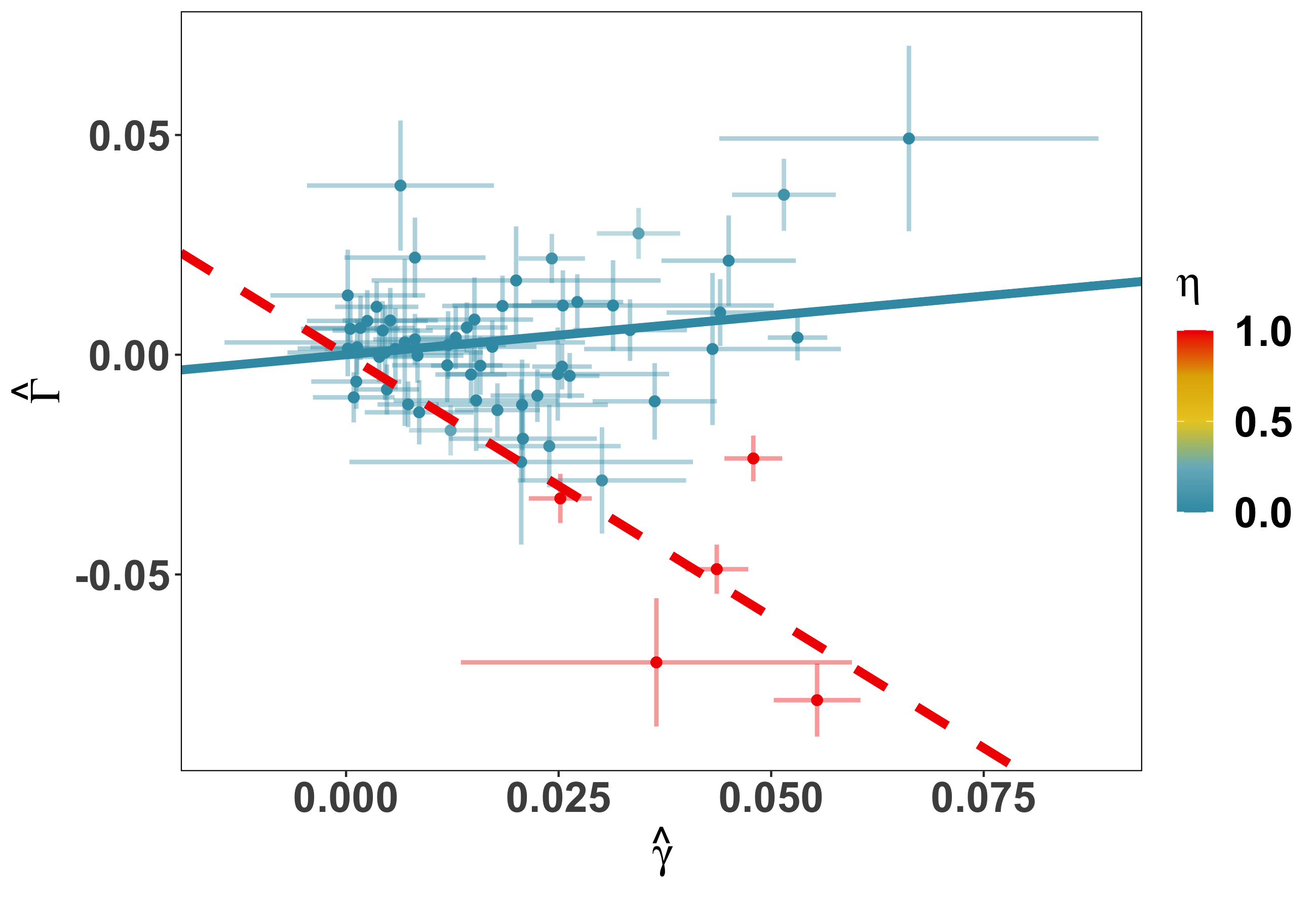
Figure 1: Scatter plot of $\widehat{\Gamma}_{k}$ against $\widehat{\gamma}_{k}$ between CAD and HDL-c. The vertical and horizontal segments represent the standard errors of $\widehat{\Gamma}_{k}$ and $\widehat{\gamma}_{k}$, respectively, at each point. To ease the presentation, we orient the reference alleles so that $\widehat{\gamma}_{k}$ is positive. For each data point, we use a spectrum of color bar to represent the mean value of latent indicators $\eta_{k}$. The blue line represents the causal effect $\hat{\beta}_{0}$ of HDL-c on CAD while the red line represents the nuisance parameter $\hat{\beta}_{1}$, see Eqn. 11.

Next we introduce a real data example that is used in the real data analysis. In this example, we are interested in estimating the causal effect of high-density lipoprotein cholesterol (HDL-c) on coronary artery disease (CAD). We obtained summary statistics from three GWASs without overlapping samples, see Table S2 in the Supplementary document.

Using HDL-c from Biobank Janpan [22] as a screening dataset, we selected 62 SNPs that have $p$-value less than $1\times 10^{-6}$ and uncorrelated (through SNP clumping; [31]). We then obtain the summary statistics $\{\widehat{\gamma}_{k},\widehat{\mathbf{s}}_{\gamma_{k}}^{2}\}$ and $\{\widehat{\Gamma}_{k},\widehat{\mathbf{s}}_{\Gamma_{k}}^{2}\}$, $k=1,\dots p$, for the SNP-HDL-c and and SNP-CAD, respectively. The scatter plot of $\widehat{\Gamma}_{k}$ against $\widehat{\gamma}_{k}$ for the 62 pairs of genetic effects with their standard errors is shown in Figure 1. By assuming the systematic independent horizontal pleiotropy (IHP), a linear relationship 2 can be applied to estimate causal effect $\beta_{0}$. However, due to CHP, there exists heteroscedasticity in this linear relationship. With larger $\widehat{\gamma}_{k}$, the variance of $\widehat{\Gamma}_{k}$ becomes larger. The statistical method should overcome this heteroscedasticity to produce robust causal estimates.

1.3 Methodological challenges and organization of the paper

Similar to its related IV methods, how to correct for CHP or correlated direct effects remains the biggest challenge for MR methods using GWAS summary statistics. As discussed in Section 1.1, there exists non-identifiability issues when we use a bivariate normal distribution for $\gamma_{k}$ and $\alpha_{k}$. To tackle this issue, we propose a strategy using a mixture of linear regressions via orthogonal projection assuming the horizontal pleiotropy is sparse. In general, this strategy can be applied to other IV methods to mitigate the impact of correlated direct effects.

Compared to IV methods and MR methods that use the individual-level data, most of classical MR methods for summary data cannot handle the correlations among instrumental variants. Usually, two variants close in distance tend to have high correlations. Moreover, these correlations decay exponentially in genetic distance. Because of correlations among genetic variants, it is not valid to use i.i.d. normal distribution (1) for GWAS summary statistics from a dense set of SNPs. Recently, we developed MR-LDP [9] to infer causal effects using correlated weak instrumental variants accounting for both linkage disequilibrium and IHP. MR methods using correlated genetic variants will improve the statistical efficiency for point estimation. To model summary statistics from correlated SNPs, the key is to use multivariate normal distributions to approximate the joint distributions of $\widehat{\bm{\gamma}}$ and $\widehat{\bm{\Gamma}}$. The details of this approximated likelihood for GWAS summary statistics are given in the Supplementary document.

In this paper, we propose a unified and statistically efficient two-sample MR method to account for CHP using weak instrumental variants. To ease the presentation, we will consider the following two nested models using GWAS summary statistics:
MODEL 1 (MR-Corr). Accounting for CHP using independent instrumental variants.
MODEL 2 (MR-Corr²). Accounting for CHP using correlated instrumental variants.

The rest of the paper is organized as follows. In Section 2, we first review the linear structural models to estimate causal effects followed by introducing the mixture of linear regressions via orthogonal projection. We also introduce MR-Corr and MR-Corr² methods in this Section. In Section 3, we connect MR-Corr with existing methods. In Section 4, we perform simulation studies to benchmark the performance of MR-Corr². In Section 5, we first apply the proposed method for the analysis of a real validation using the height-height example, and then apply MR-Corr² to analyze GWAS summary statistics from two sets of traits.

2 Methods

2.1 Linear structural models and MR

In this Section, we illustrate how MR methods work in the absence/presence of IHP using linear structural models [3, 41].

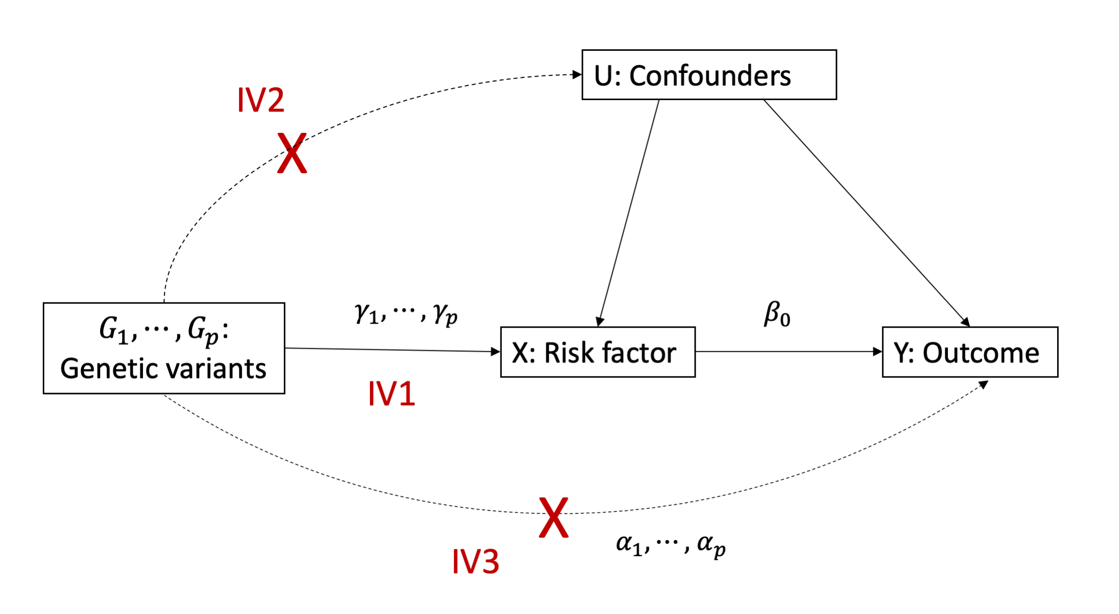
Figure 2: Direct acyclic graph of MR and three IV assumptions. IV1: genetic variants ($G_{k}$s) are associated with the exposure (relevance); IV2: $G_{k}$s are not associated with unobserved confounders (independence); IV3: $G_{k}$s have no direct effects on the outcome (exclusion). To relax the exclusion assumption (IV3), most methods assume the InSide condition that $\gamma_{k}$ and $\alpha_{k}$ are independent.

In MR analysis, we are interested in inferring causal relationship between an exposure $X$ and an outcome $Y$, with unobserved confounding factors $U$. The classical MR analysis obeys the following three assumptions in the IV methods, as shown in Figure 2:

1. The relevance assumption: The instrument $G$ is associated with the exposure $X$.

2. The independence assumption: $G$ is independent of confounders $U$.

3. The exclusion assumption: $G$ affects the outcome $Y$ only through the exposure $X$.

Assuming the validity of instrumental variants, we begin with the linear structural model,

$$X=\sum_{k=1}^{p}\gamma_{k}G_{k}+\eta_{x}U+\epsilon_{x},\quad Y=\beta_{0}X+\eta_{y}U+\epsilon_{y},$$ (3)

where $\beta_{0}$ is the causal effect of interest, $\eta_{x}$ and $\eta_{y}$ are effects of confounding factors on exposure and outcome, respectively, $\epsilon_{x}$ and $\epsilon_{y}$ are independent random noises, $(\epsilon_{x},\epsilon_{y})\perp\!\!\!\perp(G_{1},\dots,G_{p},U)$, $\epsilon_{x}\perp\!\!\!\perp\epsilon_{y}$, and $U\perp\!\!\!\perp(G_{1},\dots,G_{p})$. In two-sample MR, we observe two independent samples with sample sizes $n_{x}$ and $n_{y}$ for $(X,G_{1},\dots,G_{p})$ and $(Y,G_{1},\dots,G_{p})$, respectively. Clearly, Eqn. (3) satisfying the exclusion assumption as $(G_{1},\dots,G_{p})\perp\!\!\!\perp Y|X$. By replacing $X$ in the second equation with the first equation in Eqn. (3), we have

$$Y=\sum_{k=1}^{p}\beta_{0}\gamma_{k}G_{k}+(\beta_{0}\eta_{x}+\eta_{y})U+\beta_{0}\epsilon_{x}+\epsilon_{y}.$$

Therefore, the effect $\Gamma_{k}$ of variant $k$ on the health outcome can be written as

$$\Gamma_{k}=\beta_{0}\gamma_{k},\forall k=1,\dots,p.$$ (4)

In practice, the exclusion assumption can be easily violated because of ubiquitous horizontal pleiotropy or direct effects. Similar to Eqn. (3), the linear structural model incorporating horizontal pleiotropy $\alpha_{k}$, on each variant $k$ can be written as

$$X=\sum_{k=1}^{p}\gamma_{k}G_{k}+\eta_{x}U+\epsilon_{x},\quad Y=\sum_{k=1}^{p}\alpha_{k}G_{k}+\beta_{0}X+\eta_{y}U+\epsilon_{y},$$ (5)

Again, by replacing $X$ in the second equation with the first equation in Eqn. (5), we have

$$Y=\sum_{k=1}^{p}(\beta_{0}\gamma_{k}+\alpha_{k})G_{k}+(\beta_{0}\eta_{x}+\eta_{y})U+\beta_{0}\epsilon_{x}+\epsilon_{y}.$$

Thus, the effect $\Gamma_{k}$ of variant $k$ on the health outcome can be written as Eqn. (2).

In practice, performing causal inference using either Eqn. (3) or Eqn. (5) is impractical as it requires individual-level data, Fortunately, GWAS summary statistics are publicly accessible. Suppose that we obtain summary statistics for health risk factor and (disease) outcome as $\{\widehat{\gamma}_{k},\widehat{\mathbf{s}}_{\gamma_{k}}^{2}\}$ and $\{\widehat{\Gamma}_{k},\widehat{\mathbf{s}}_{\Gamma_{k}}^{2}\},\forall k=1,\dots,p$, respectively, from two independent samples, where $p$ is the number of genetic variants. To ease the presentation, we first consider summary statistics for a set of independent genetic variants by SNP clumping. The corresponding MR-Corr model is introduced in Section 2.3. Later, we extend our model to incorporate genetic variants within LD and introduce MR-Corr² in Section 2.4. For independent genetic variants, their distributions for summary statistics can be written as Eqn. (1). To further account for horizontal pleiotropy, various MR methods have been developed to estimate the causal effect $\beta_{0}$ by assuming that $\bm{\alpha}\perp\!\!\!\perp\bm{\gamma}$ (the InSIDE condition). In genetic studies, the InSIDE condition may not hold due to heteroscedasticity in $\bm{\gamma}$ and $\bm{\alpha}$. In Section 3, we provide a perspective to treat CHP by connecting our methods with CAUSE.

Remark 1: From the linear structural model (3), we know that when the classical IV assumptions (Figure 2) hold, there exists a deterministic linear relationship between $\Gamma_{k}$ and $\gamma_{k}$, $\forall k=1,\dots,p$, i.e., Eqn. (4). The resulting absolute correlation, denoted as $|\rho_{g}|$, between $\bm{\Gamma}$ and $\bm{\gamma}$ will be the exact 1, which is unrealistic as the absolute value of genetic correlation between any two distinct traits can never be 1. Note that $\rho_{g}$ is different from $\rho_{\alpha\gamma}$, which is the correlation between $\bm{\gamma}$ and $\bm{\alpha}$. On the other hand, the linear relationship with systematic IHP in Eqn. (2) is more flexible, resulting a correlation that $|\rho_{g}|<1$.

2.2 Mixture of linear regressions via orthogonal projection

To correct for CHP, we develop a strategy using a mixture of linear regressions (MLR) via orthogonal projection. Our key idea is based on the following observation. For the ease of presentation, we assume that instrumental variants are independent here and will generalize this strategy to handle correlated instrumental variants in Section 2.4. Suppose that the effects of genetic variant on exposure and horizontal pleiotropy follow a bivariate normal distribution for each variant $k$,

$$\left(\begin{array}[]{c}\gamma_{k}\\ \alpha_{k}\end{array}\right)\sim\mbox{ $\mathcal{N}$}\left(\bm{0},\left(\begin{array}[]{cc}\sigma_{\bm{\gamma}}^{2},&\rho_{\alpha\gamma}\ \sigma_{\bm{\gamma}}\sigma_{\bm{\alpha}_{0}}\\ \rho_{\alpha\gamma}\ \sigma_{\bm{\gamma}}\sigma_{\bm{\alpha}_{0}},&\sigma_{\bm{\alpha}_{0}}^{2}\end{array}\right)\right),$$ (10)

where $\rho_{\alpha\gamma}$ is the correlation between $\gamma_{k}$ and $\alpha_{k}$. Clearly, from Eqn. (10), we have

$$\gamma_{k} \sim \mbox{ $\mathcal{N}$}(0,\sigma_{\bm{\gamma}}^{2}),$$

$$\alpha_{k} = \rho_{\alpha\gamma}\frac{\sigma_{\bm{\alpha}0}}{\sigma_{\bm{\gamma}}}\gamma_{k}+\sqrt{1-\rho_{\alpha\gamma}^{2}}\sigma_{\bm{\alpha}0}Z_{k}\stackrel{{\scriptstyle\mbox{{\tiny def}}}}{{=}}c\gamma_{k}+\widetilde{\alpha}_{k},$$

where $Z_{k}\perp\!\!\!\perp\gamma_{k}$ and $Z_{k}\sim\mbox{ $\mathcal{N}$}(0,1)$. In this way, $\alpha_{k}$ can be decomposed into two parts, one is in a linear relationship with $\gamma_{k}$ and the other is independent of $\gamma_{k}$, i.e., $\widetilde{\alpha}_{k}\perp\!\!\!\perp\gamma_{k}$ and $\widetilde{\alpha}_{k}\sim\mbox{ $\mathcal{N}$}(0,\sigma_{\bm{\alpha}}^{2})$. We can further parameterize the causal relationship for genetic variant $k$ as follows

$$\Gamma_{k}=\left\{\begin{aligned} &\beta_{0}\gamma_{k},&&\widetilde{\alpha}_{k}=0\\ &\beta_{1}\gamma_{k}+\widetilde{\alpha}_{k},&&\widetilde{\alpha}_{k}\neq 0,\end{aligned}\right.$$ (11)

where $\beta_{0}$ is the causal effect of interest and $\beta_{1}=\beta_{0}+\rho_{\alpha\gamma}\frac{\sigma_{\bm{\alpha}0}}{\sigma_{\bm{\gamma}}}$ is a nuisance parameter. Therefore, to remove the impact of CHP in Eqn. (10) is equivalent to identifying zero orthogonal projection of $\alpha_{k}$, namely $\widetilde{\alpha}_{k}=0$, in Eqn. (11). For this purpose, we may apply a spike-slab prior on $\widetilde{\alpha}_{k}$ [19]. This observation motivates us to model $\Gamma_{k}$ as a mixture of two linear relationships with $\gamma_{k}$ depending on the value of $\widetilde{\alpha}_{k}$. Thus, using MLR strategy, the causal effect $\beta_{0}$ can be estimated consistently by removing the impact of CHP as long as correlation $\rho_{\alpha\gamma}$ is not too close to 1 or -1.

2.3 MR-Corr model

In practice, the InSIDE condition may not hold due to the pervasive heteroscedasticity among complex traits, resulting in correlations between horizontal pleiotropy, $\bm{\alpha}$, and effects on exposure, $\bm{\gamma}$. As shown in our simulations (Figure 4), a small deviation from zero correlation may lead to severe inflation in type-I error, making MR methods not correcting for CHP less reliable.

Here, we consider a Bayesian MR method via the MLR strategy to correct for CHP using independent instrumental variants. Assuming the independence among instrumental variants as well as independent samples for SNP-exposure and SNP-outcome, for each variant $k$, $\widehat{\gamma}_{k}$ and $\widehat{\Gamma}_{k}$ are i.i.d. distributed as Eqn. (1). By introducing a latent indicator $\eta_{k}$ for each variant $k$, we assign a spike-slab prior on $\widetilde{\alpha}_{k}$ [19, 35],

$$\widetilde{\alpha}_{k}\sim\left\{\begin{aligned} &\mbox{ $\mathcal{N}$}(0,\sigma_{\bm{\alpha}}^{2}),&&\eta_{k}=1\\ &\delta_{0}(\alpha_{k}),&&\eta_{k}=0,\end{aligned}\right.$$

where $\mbox{ $\mathcal{N}$}(0,\sigma_{\bm{\alpha}}^{2})$ denotes a normal distribution with mean 0 and variance $\sigma_{\bm{\alpha}}^{2}$, $\delta_{0}$ denotes the Dirac delta function at zero, $\eta_{k}=1$ means the $k$-th genetic variant present nonzero orthogonal projected pleiotropic effect, and $\eta_{k}=0$ means zero orthogonal projected pleiotropic effect. Here, $\eta_{k}$ is a Bernoulli random variable with probability $\omega$ being 1, i.e., $\eta_{k}\sim\omega^{\eta_{k}}(1-\omega)^{1-\eta_{k}}$.

Using the reparameterization trick in Eqn. (11), the relationship between $\bm{\gamma}$ and $\bm{\Gamma}$ can be constructed linearly as

$$\Gamma_{k}=\beta_{0}(1-\eta_{k})\gamma_{k}+\beta_{1}\eta_{k}\gamma_{k}+\eta_{k}\widetilde{\alpha}_{k},$$ (12)

where $k=1,\dots,p$ and $\bm{\gamma}\perp\!\!\!\perp\widetilde{\bm{\alpha}}$. Then, we propose the following hierarchical Bayesian model for MR-Corr with MLR strategy to account for CHP,

$$\widehat{\Gamma}_{k}|\Gamma_{k}\stackrel{{\scriptstyle i.i.d.}}{{\sim}}\mathcal{N}(\Gamma_{k},\widehat{\mathbf{s}}_{\Gamma_{k}}^{2}),\quad\widehat{\gamma}_{k}|\gamma_{k}\stackrel{{\scriptstyle i.i.d.}}{{\sim}}\mathcal{N}(\gamma_{k},\widehat{\mathbf{s}}_{\Gamma_{k}}^{2}),$$

$$\Gamma_{k}=\beta_{0}(1-\eta_{k})\gamma_{k}+\beta_{1}\eta_{k}\gamma_{k}+\eta_{k}\widetilde{\alpha}_{k},$$

$$\gamma_{k}|\sigma_{\gamma}^{2}\stackrel{{\scriptstyle i.i.d.}}{{\sim}}\mathcal{N}(0,\sigma^{2}_{\gamma}),\quad\widetilde{\alpha}_{k}|\sigma_{\alpha}^{2}\stackrel{{\scriptstyle i.i.d.}}{{\sim}}\mathcal{N}(0,\sigma^{2}_{\alpha}),\quad\eta_{k}|\omega\stackrel{{\scriptstyle i.i.d.}}{{\sim}}\omega^{\eta_{k}}(1-\omega)^{1-\eta_{k}},$$

$$\sigma^{2}_{\gamma}\sim\mathcal{IG}(a_{\gamma},b_{\gamma}),\quad\sigma^{2}_{\alpha}\sim\mathcal{IG}(a_{\alpha},b_{\alpha}),\quad\omega\sim Beta(a,b),$$ (13)

where Jeffreys non-informative priors are used for both $\beta_{0}$ and $\beta_{1}$ and a spike-slab prior (2.3) is reprameterized as $\widetilde{\alpha}_{k}\omega_{k}$. The detailed Gibbs sampling algorithm with pseudo codes can be found in the Supplementary document.

2.4 MR-Corr² model

As MR-Corr (2.3) assumes the SNPs are independent, it does not work for instrumental variants in LD. To further incorporate SNPs in LD for MR analysis, we develop MR-Corr² here. The key is to build a joint summary statistics distribution for correlated SNPs. For this purpose, we use the approximated distribution for summary statistics [42, 18],

$$\widehat{\bm{\gamma}}|\bm{\gamma},\widehat{\mathbf{R}},\widehat{\mathbf{S}}_{\gamma} \sim \mbox{ $\mathcal{N}$}(\widehat{\mathbf{S}}_{\gamma}\widehat{\mathbf{R}}\widehat{\mathbf{S}}_{\gamma}^{-1}\bm{\gamma},\widehat{\mathbf{S}}_{\gamma}\widehat{\mathbf{R}}\widehat{\mathbf{S}}_{\gamma}),$$

$$\widehat{\bm{\Gamma}}|\bm{\Gamma},\widehat{\mathbf{R}},\widehat{\mathbf{S}}_{\Gamma} \sim \mbox{ $\mathcal{N}$}(\widehat{\mathbf{S}}_{\Gamma}\widehat{\mathbf{R}}\widehat{\mathbf{S}}_{\Gamma}^{-1}\bm{\Gamma},\widehat{\mathbf{S}}_{\Gamma}\widehat{\mathbf{R}}\widehat{\mathbf{S}}_{\Gamma}),$$ (14)

where $\widehat{{\mathbf{S}}_{\gamma}}=\text{diag}([\widehat{\mathbf{s}}_{\gamma_{1}},\cdots,\widehat{\mathbf{s}}_{\gamma_{p}}])$ and $\widehat{{\mathbf{S}}_{\Gamma}}=\text{diag}([\widehat{\mathbf{s}}_{\Gamma_{1}},\cdots,\widehat{\mathbf{s}}_{\Gamma_{p}}])$ are both diagonal matrices, $\widehat{\bm{\gamma}}=[\widehat{\gamma}_{1},\dots,\widehat{\gamma}_{p}]^{T}$, $\widehat{\bm{\Gamma}}=[\widehat{\Gamma}_{1},\dots,\widehat{\Gamma}_{p}]^{T}$, $\bm{\gamma}=[\gamma_{1},\dots,\gamma_{p}]^{T}$, $\bm{\Gamma}=[\Gamma_{1},\dots,\Gamma_{p}]^{T}$. Given that sample size $n$ is large enough and the trait is highly polygenic, i.e., the squared correlation coefficient between the trait and each genetic variant is close to zero, Zhu and Stephens [42] showed that difference between the likelihoods based on the individual-level data and summary statistics is some constant that does not depend on $\bm{\gamma}$ under some regularity conditions (See Table 1 in [42] and Table S4 in [39] for numerical justifications). Details for this approximated distribution can be found in Section S1.1.

As GWAS summary statistics does not contain any information for the correlation $\widehat{\mathbf{R}}$, we use an additional independent sample as reference data to estimate this correlation $\widehat{\mathbf{R}}^{\mathrm{ref}}$. In [18], we theoretically analyzed the impact of using reference sample to estimate this correlation for $l_{1}$ penalization and empirical results in [42, 18, 9] show that the distribution for summary statistics approximates the individual-level one well. The details for the choice of LD can be found in Section Section S1.2.

Next, we show how to use MLR strategy for correlated SNPs. Clearly, when there is a single variant $k$ with nonzero direct effect $\alpha_{k}$, the direct effect for a nearby variant $k^{\prime}$ would be nonzero as well. This is because variants $k$ and $k^{\prime}$ from the same LD are highly correlated. Moreover, LD across the genome can be partitioned into independent blocks. SNPs within the same block are correlated but SNPs from different blocks are independent. Thus, the orthogonal projection $\widetilde{\alpha}_{k}$ should be in a group manner. Here, we introduce a group-level latent status $\eta_{l}$, indicating whether genetic variants within the $l$-th block present nonzero horizontal pleiotropy and assign a spike-slab prior on $\widetilde{\alpha}_{lk}$ [19, 35],

$$\widetilde{\alpha}_{lk}\sim\left\{\begin{aligned} &\mbox{ $\mathcal{N}$}(0,\sigma_{\bm{\alpha}}^{2}),&&\eta_{l}=1\\ &\delta_{0}(\alpha_{lk}),&&\eta_{l}=0,\end{aligned}\right.$$ (15)

where $\mbox{ $\mathcal{N}$}(0,\sigma_{\bm{\alpha}}^{2})$ denotes a normal distribution with mean 0 and variance $\sigma_{\bm{\alpha}}^{2}$, $\delta_{0}$ denotes the Dirac delta function at zero, $\eta_{l}=1$ means variants within the $l$-th block present nonzero orthogonal projected pleiotropic effects or $\eta_{l}=0$ means orthogonal projected pleiotropic effects from variants within block $l$ are all zero. Here, $\eta_{l}$ is a Bernoulli random variable with probability $\omega$ being 1, $\eta_{l}\sim\omega^{\eta_{l}}(1-\omega)^{1-\eta_{l}}$.

Using the reparameterization trick in Eqn. (15), the relationship between $\bm{\gamma}$ and $\bm{\Gamma}$ can be constructed linearly as:

$$\Gamma_{lk}=\beta_{0}(1-\eta_{l})\eta_{l}\gamma_{lk}+\beta_{1}\eta_{l}\gamma_{lk}+\eta_{l}\widetilde{\alpha}_{lk},$$ (16)

where $l=1,\dots,L$, $k=1,\dots,p_{l}$ and $\gamma_{lk}\perp\!\!\!\perp\widetilde{\alpha}_{lk}$. Then we propose the following hierarchical Bayesian model for MR-Corr²,

$$\widehat{\bm{\gamma}}|\bm{\gamma},\widehat{\mathbf{R}},\widehat{\mathbf{S}}_{\gamma}\sim\mbox{ $\mathcal{N}$}(\widehat{\mathbf{S}}_{\gamma}\widehat{\mathbf{R}}\widehat{\mathbf{S}}_{\gamma}^{-1}\bm{\gamma},\widehat{\mathbf{S}}_{\gamma}\widehat{\mathbf{R}}\widehat{\mathbf{S}}_{\gamma}),$$ (17)

$$\widehat{\bm{\Gamma}}|\bm{\Gamma},\widehat{\mathbf{R}},\widehat{\mathbf{S}}_{\Gamma}\sim\mbox{ $\mathcal{N}$}(\widehat{\mathbf{S}}_{\Gamma}\widehat{\mathbf{R}}\widehat{\mathbf{S}}_{\Gamma}^{-1}\bm{\Gamma},\widehat{\mathbf{S}}_{\Gamma}\widehat{\mathbf{R}}\widehat{\mathbf{S}}_{\Gamma}),$$

$$\Gamma_{lk}=\beta_{0}(1-\eta_{l})\eta_{l}\gamma_{lk}+\beta_{1}\eta_{l}\gamma_{lk}+\eta_{l}\widetilde{\alpha}_{lk},$$

$${\color[rgb]{0,0,0}\gamma_{lk}|\sigma_{\gamma}^{2}\stackrel{{\scriptstyle i.i.d.}}{{\sim}}\mathcal{N}(0,\sigma_{\gamma}^{2}),\quad\widetilde{\alpha}_{lk}|\sigma_{\alpha}^{2}\stackrel{{\scriptstyle i.i.d.}}{{\sim}}\mathcal{N}(0,\sigma_{\alpha}^{2}),\quad\eta_{l}|\omega\stackrel{{\scriptstyle i.i.d.}}{{\sim}}\omega^{\eta_{l}}(1-\omega)^{1-\eta_{l}},}$$

$$\sigma^{2}_{\gamma}\sim\mathcal{IG}(a_{\gamma},b_{\gamma}),\quad\sigma^{2}_{\alpha}\sim\mathcal{IG}(a_{\alpha},b_{\alpha}),\quad\omega\sim Beta(a,b).$$

The corresponding parallel Gibbs sampling algorithm with pseudo codes can be found in the Supplementary document.

3 Connections with Existing Methods

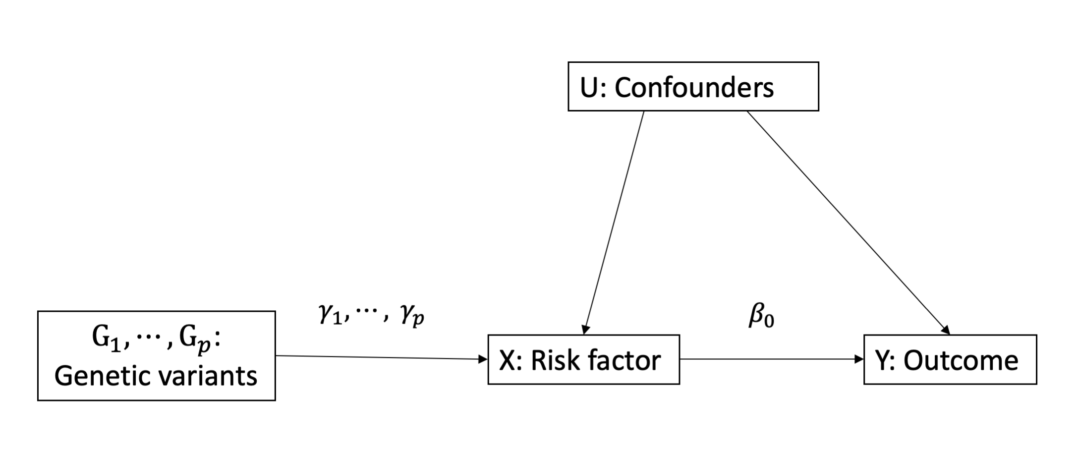
(a) Mechanism 1

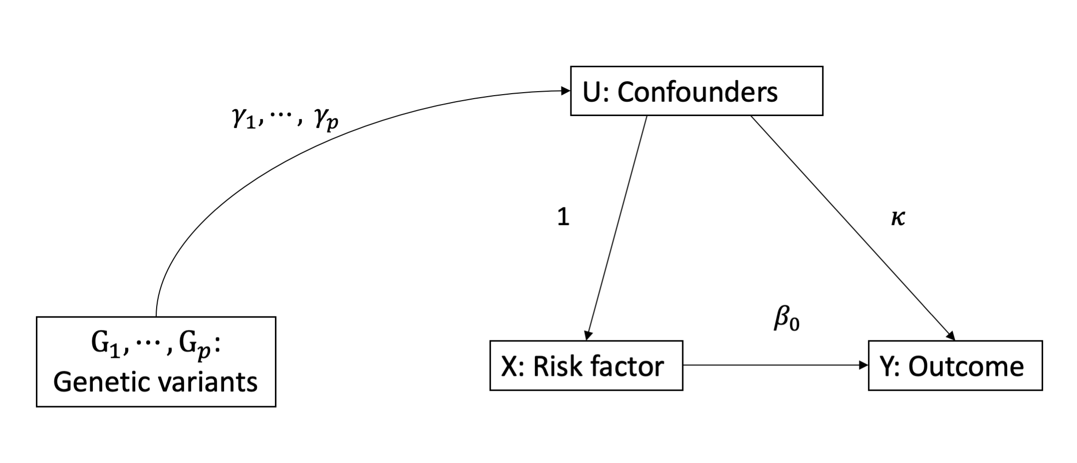
(b) Mechanism 2

Figure 3: The causal mechanisms between exposure $X$ and outcome $Y$. Mechanism 1 is the classical one while mechanism 2 refers to correlated pleiotropy.

Recently, [27] proposed a CAUSE method to address the problem that genetic variants affect both the exposure and outcome through a heritable shared factor and thus there are two mechanisms that SNPs affect an outcome as shown in Figure 3. Here, to ease the illustration, we consider only correlated pleiotropy for independent SNPs as shown in Figure 3(b). By assuming the effect of confounding factor $U$ on exposure $X$ is scaled to 1 and considering the effect of $U$ on $Y$ is $\kappa$, the relationship between $\gamma_{k}$ and $\Gamma_{k}$ without considering horizontal pleiotropy can be written as

$$\Gamma_{k}=\beta_{0}\gamma_{k}+\eta_{k}\kappa\gamma_{k},$$ (18)

where $\eta_{k}$ is an indicator of whether $G_{k}$ affects $U$ that has different meaning in MR-Corr. Using the fact that $\beta_{1}=\beta_{0}+\kappa$, simple algebra shows that when $\widetilde{\alpha}_{k}\rightarrow 0$, Eqn. (12) reduces to Eqn. (18). Thus, the CAUSE model with only correlated pleiotropy can be taken as an extreme case of MR-Corr. By using the mechanism of CHP, the term $\kappa\gamma_{k}$ in Eqn. (18) can be taken as horizontal pleiotropy but is fully correlated with $\gamma_{k}$ with $|\rho_{\alpha\gamma}|=1$. This only happens when there is a single confounding factor $U$ that affects both the exposure and outcome. In this case, $\widetilde{\alpha}_{k}$ = 0 exactly as long as this single confounder has a scaled effect $\kappa$ on $Y$. However, when there are multiple confounding factors ($U_{1},\dots,U_{q})$ and these confounding factors affect the outcome through some mediators as well as present direct effects, the relationship between these confound factors and outcome $Y$ would therefore show deviations from the deterministic linear relationship with random errors. These random errors could represent the independent direct effects between multiple confounders and outcome. In this case, $\widetilde{\alpha}_{k}$ would not be 0 and Eqn. (12) holds.

Moreover, the identifiability of CAUSE model is up to the identifiability of indicator $\eta_{k}$. Moreover, the consistency of estimating causal effects $\beta_{0}$ depends on how well one can estimate $\eta_{k}$. Compared to identify which mechanism is applied to a genetic variant as in CAUSE, identifying whether $\widetilde{\alpha}_{k}$ is 0 is much easier and also identifiable. As our methods avoid the case that $|\rho_{\alpha\gamma}|$ lies on the boundary, there will be no identifiablity problems.

Because of the existence of CHP, in many cases, one would observe that many SNPs do not obey either Eqn. (4) or Eqn. (2). RAPS and BWMR tackle this issue by treating these SNPs as idiosyncratic outliers. Despite the fact that estimating causal effect using either Eqn. (4) or Eqn. (2) is similar to performing a linear regression, treating SNPs that do not obey these relationships as idiosyncratic outliers is not justified. This is because we work on the true effect sizes $\bm{\gamma}$ and $\bm{\Gamma}$ without measurement errors. There should exist mechanisms that cause this phenomenon and CHP is one of them. As one can observed in Figure 1, when the value of $\widehat{\gamma}_{k}$ is large, the variation of $\widehat{\Gamma}_{k}$ is large, causing the variance of “residuals" to increase with the ’predictor variable’ $\widehat{\gamma}_{k}$. In the literature on linear regression, variance-stabilizing transformation can be applied, e.g. Box-Cox transformation [34]. However, this technique is not applicable in MR as we work on unobserved estimated effects $\widehat{\bm{\gamma}}$ and $\widehat{\bm{\Gamma}}$ instead of the true effects of them. Fortunately, only SNPs with CHP would present this problem as idiosyncratic outliers and MLR strategy can effectively mitigate the impact from these SNPs.

4 Simulation Studies

4.1 Simulation settings

In this section, we performed simulation studies to evaluate the performance of MR-Corr². In this simulation, we considered two scenarios: 1) The generative model for individual-level data generated as Eqn. 19 with correlated $\bm{\alpha}$ and $\bm{\gamma}$; 2) The correlated pleiotropy model in CAUSE setting as shown in Figure 3.

In Scenario 1, we used the following structural model to generate individual-level data

$${\mathbf{x}}={\mathbf{G}}_{1}\bm{\gamma}+{\mathbf{U}}_{x}\bm{\eta}_{x}+{\mathbf{e}}_{1},\quad{\mathbf{y}}=\beta_{0}{\mathbf{x}}+{\mathbf{G}}_{2}\bm{\alpha}+{\mathbf{U}}_{y}\bm{\eta}_{y}+{\mathbf{e}}_{2},$$ (19)

where ${\mathbf{G}}_{1}\in\mathbb{R}^{n_{1}\times p}$ and ${\mathbf{G}}_{2}\in\mathbb{R}^{n_{2}\times p}$ are genotype matrices for two samples, ${\mathbf{U}}_{x}\in\mathbb{R}^{n_{1}\times r}$ and ${\mathbf{U}}_{y}\in\mathbb{R}^{n_{2}\times r}$ are matrices for confounding variables, $n_{1}$ and $n_{2}$ are the corresponding sample sizes that are set at 20,000, $p$ is the number of genetic variants, ${\mathbf{x}}\in\mathbb{R}^{n_{1}\times 1}$ is the exposure vector, ${\mathbf{y}}\in\mathbb{R}^{n_{2}\times 1}$ is the outcome vector, and ${\mathbf{e}}_{1}$ and ${\mathbf{e}}_{2}$ are independent random errors. Note that Eqn. (19) is the sample version of the linear structural model (5).

In Scenario 2, we first generated $q$ from $Beta(1,10)$ as in [27]. Then we divided all $p$ genetic variants into two groups corresponding to two mechanisms in Figure 3(a) and (b), respectively, with proportion $1-q$ and $q$. For genetic variants with proportion $1-q$ in mechanism 1 (Figure 3(a)), the exposure vector was generated as

$${\mathbf{x}}^{1}={\mathbf{G}}_{1}^{1}\bm{\gamma}^{1}+{\mathbf{U}}_{x}^{1}\bm{\eta}_{x}^{1}+{\mathbf{e}}_{1}^{1},$$

where subscript indicates which mechanism is active, ${\mathbf{G}}_{1}^{1}$ is the genotype matrix in SNP-exposure sample for the genetic variants from mechanism 1 and $\bm{\gamma}^{1}$ is the corresponding coefficient vector. For the remaining SNPs, the exposure vector was generated as

$${\mathbf{U}}_{x}^{2}={\mathbf{G}}_{1}^{2}\bm{\gamma}^{2}+{\mathbf{e}}_{{\mathbf{U}}},\quad{\mathbf{x}}^{2}={\mathbf{U}}_{x}^{2}+{\mathbf{e}}_{1}^{2},$$

where ${\mathbf{G}}_{1}^{2}$ is the genotype matrix in SNP-exposure sample for the genetic variants from mechanism 2 and $\bm{\gamma}^{2}$ is the corresponding coefficient vector. By combining these two mechanisms, the outcome vector can be generated as

$${\mathbf{x}}={\mathbf{x}}^{1}+{\mathbf{x}}^{2},\quad{\mathbf{y}}=\beta_{0}{\mathbf{x}}+{\mathbf{G}}_{2}\bm{\alpha}+{\mathbf{U}}_{y}\bm{\eta}_{y}+{\mathbf{e}}_{2}.$$

For both scenarios, we first generated genotype matrices from multivariate normal distribution $\mbox{ $\mathcal{N}$}(\bf 0,\bm{\Sigma}(\rho))$, where $\bm{\Sigma}(\rho)$ is a block autoregressive (AR) with $\rho=0.4$, or $0.8$ representing moderate or strong LD, respectively. The genotype matrices were then categorized into dosage values $\{0,1,2\}$ according to the Hardy-Weinberg equilibrium using the minor allele frequencies drawn from a uniform distribution $\mathbb{U}(0.05,0.5)$. Moreover, we assumed that $\gamma_{k}$ and $\alpha_{k}$ from a bivariate normal distribution $\mbox{ $\mathcal{N}$}(\bf 0,\bm{\Sigma}(\rho_{\alpha\gamma}))$, where $\rho_{\alpha\gamma}$ is the correlation between $\alpha_{k}$ and $\gamma_{k}$. We varied $\rho_{\alpha\gamma}\in\{0,0.2.0.4\}$. In addition, we considered $\alpha$ to be sparse, i.e., only a fraction of $\alpha_{k}$ was from this bivariate normal distribution and others are zero. The sparsity was fixed at 10%.

For confounding variables, we sampled each column of ${\mathbf{U}}_{x}$ and ${\mathbf{U}}_{y}$ from a standard normal distribution with fixed $r=50$. For their corresponding coefficients $\bm{\eta}_{x}\in\mathbb{R}^{r\times 1}$ and $\bm{\eta}_{y}\in\mathbb{R}^{r\times 1}$, each row of $(\bm{\eta}_{x},\bm{\eta}_{y})$ was generated from a multivariate normal distribution $\mbox{ $\mathcal{N}$}(\bf 0,\bm{\Sigma}_{\eta})$, where $\bm{\Sigma}_{\eta}$ is a two-by-two matrix with diagonal elements set as 1 and off-diagonal elements set as 0.8.

We then conducted single-variant analysis to obtain the summary statistics for SNP-exposure and SNP-outcome, $\{\widehat{\gamma}_{k},\widehat{s}_{\bm{\gamma}k}^{2}\}_{k=1,\cdots,p}$ and $\{\widehat{\Gamma}_{k},\widehat{s}_{\bm{\Gamma}k}^{2}\}_{k=1,\cdots,p}$, respectively. In simulations, we controlled the signal magnitude for both $\bm{\gamma}$ and $\bm{\alpha}$ using their corresponding heritability, $h_{\bm{\gamma}}^{2}=\frac{\hbox{var}(\beta_{0}{\mathbf{G}}_{1}\bm{\gamma})}{\hbox{var}({\mathbf{y}})}$ and $h_{\bm{\alpha}}^{2}=\frac{\hbox{var}({\mathbf{G}}_{2}\bm{\alpha})}{\hbox{var}({\mathbf{y}})}$, respectively. Thus, we could control $h_{\bm{\alpha}}^{2}$ and $h_{\bm{\gamma}}^{2}$ at any value by controlling confounding variables, and the error terms, $\sigma_{{\mathbf{e}}_{1}}^{2}$ and $\sigma_{{\mathbf{e}}_{2}}^{2}$. In all settings, we fixed $h_{\bm{\gamma}}^{2}=0.1$ and varied $h_{\bm{\alpha}}^{2}\in\{0.05,0.1\}$.

4.2 Simulation results

We benchmark the performance of MR-Corr² using correlated SNPs, i.e., $\rho=0.4$ and $0.8$, in comparison with alternative methods, including MR-LDP, CAUSE, GSMR, MRMix and RAPS. In this simulation, we set the number of blocks $L$ to be 100 or 200 and the number of SNPs within a block to be 10. Thus we have $p$= 1,000 or 2,000 in total. As MR-Corr² and MR-LDP need an additional reference data to estimate LD, we generated an independent reference panel $G_{3}$ with sample size 500. Next we applied all six methods on the simulated summary statistics as shown in Section 4.1. Since MR-Corr, CAUSE, GSMR, MRMix and RAPS cannot account for strong correlated SNPs, we conducted SNP clumping to obtain independent SNPs for making fair comparisons on point estimates.

In different scenarios, we evaluated type-I error under the null that $\beta_{0}=0$ while we set $\beta_{0}=0.1$ to evaluate point estimates under the alternative. We ran 1,000 and 100 replicates to assess type-I error and point estimates, respectively. Figure 4 shows type-I error and point estimates of all methods when $\rho_{\alpha\gamma}=0.2$. As we can see, MR-Corr² can effectively control type-I error in the presence of LD with CHP in both scenarios. While the type-I error of MR-LDP is a little inflated in the second scenario, it is severely inflated in the case of Scenario 1. Using all correlated SNPs, type-I errors for GSMR, MRMix and RAPS are severely inflated. After performing SNP clumping, the inflation issue for GSMR is largely reduced but there is deflated issue for MRMix. For point estimates, MR-Corr² is unbiased for all $\rho_{\alpha\gamma}$ in both scenario and has the smallest standard errors while CAUSE is largely biased. Comparing to other alternative methods, GSMR has smaller biasedness and standard deviation for point estimates. The overall pattern is similar when $\rho_{\alpha\gamma}=0.4$ as shown in Figure S2. When $\rho_{\alpha\gamma}$ becomes larger, the inflation of type-I error for MR-LDP in Scenario 1 is more severe. This is because MR-LDP accounts for only IHP but not CHP. We also shows the results from no CHP ($\rho_{\alpha\gamma}=0$) in Figure S1. When there is no CHP, all methods perform well in Scenario 1 but point estimates from MR-LDP and RAPS are biased in Scenario 2.

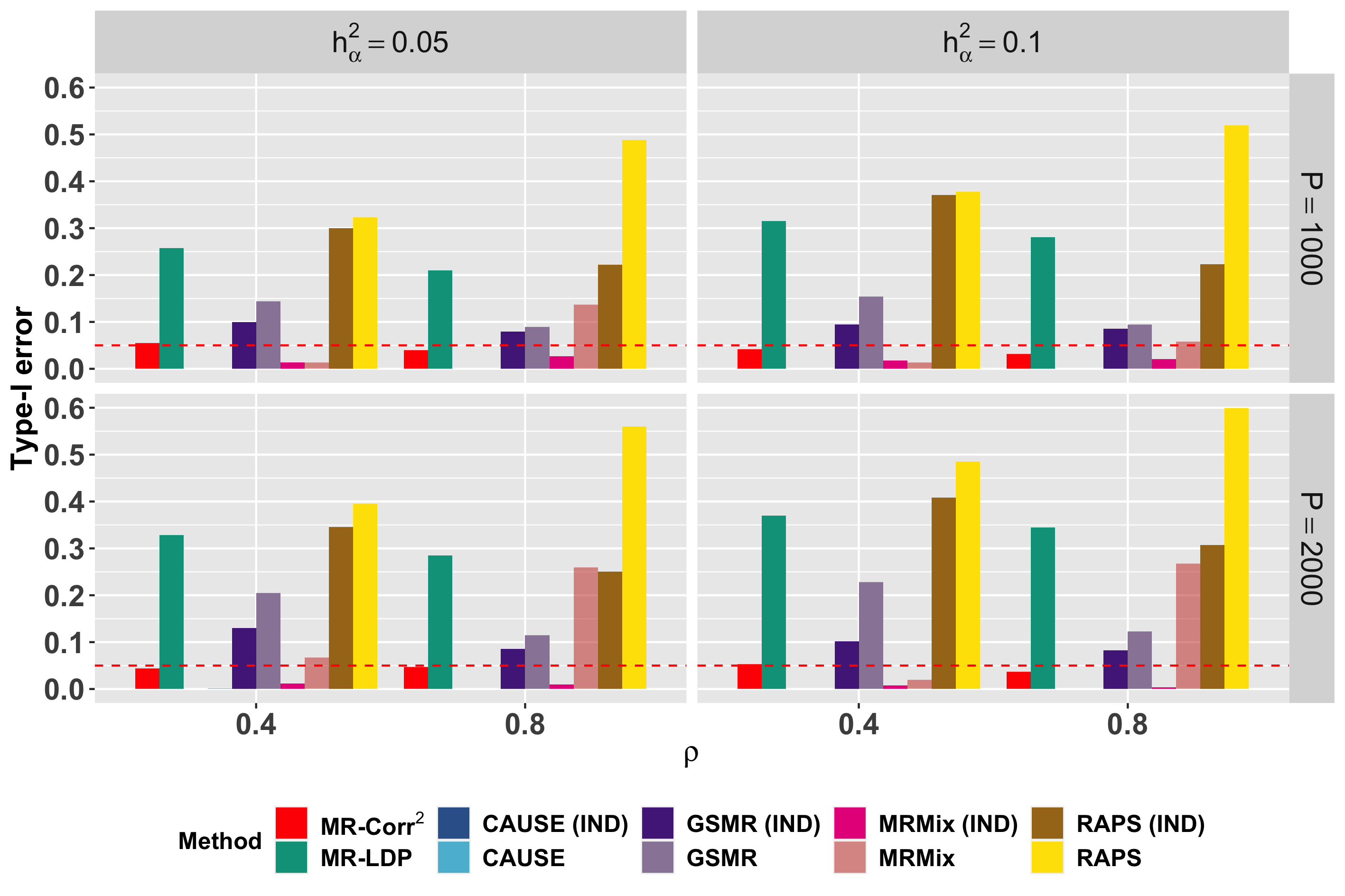
(a) Type-I error

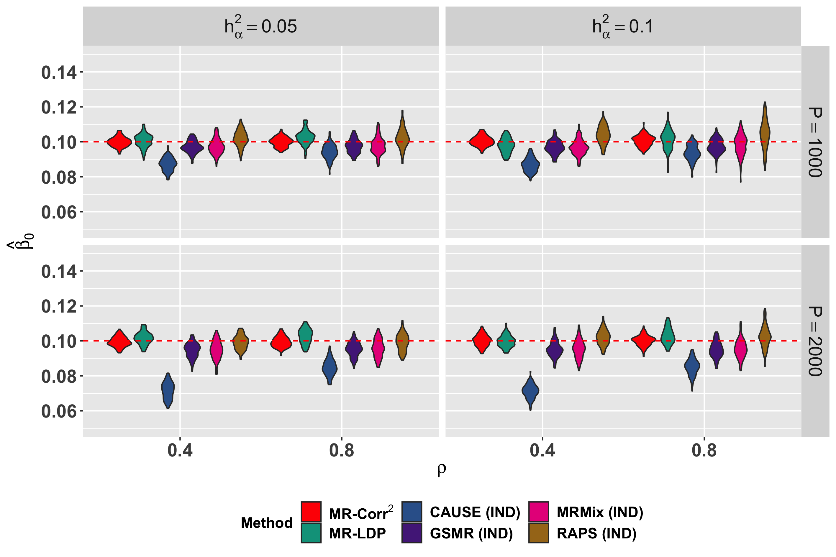
(b) Point estimate

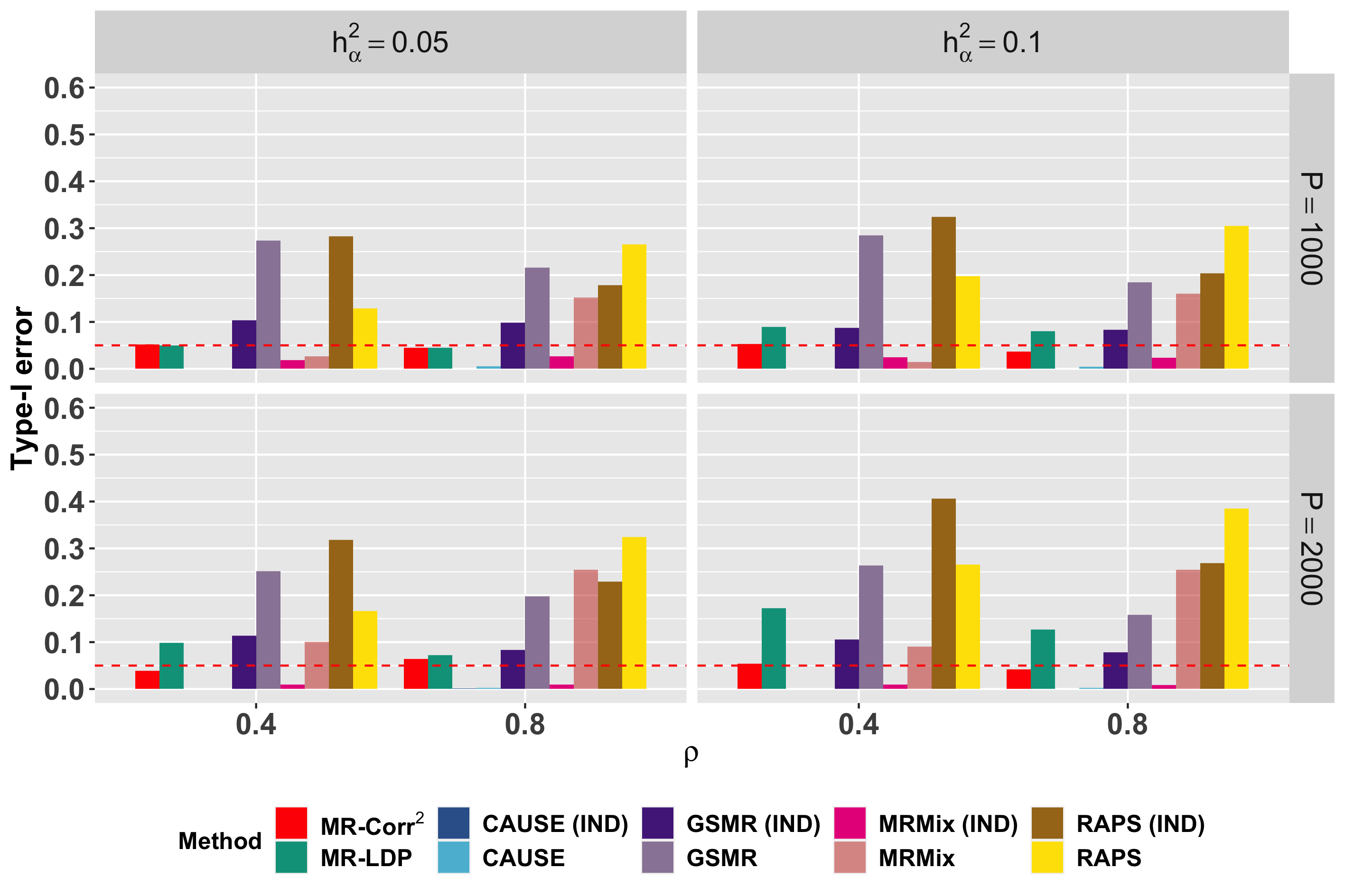
(c) Type-I error

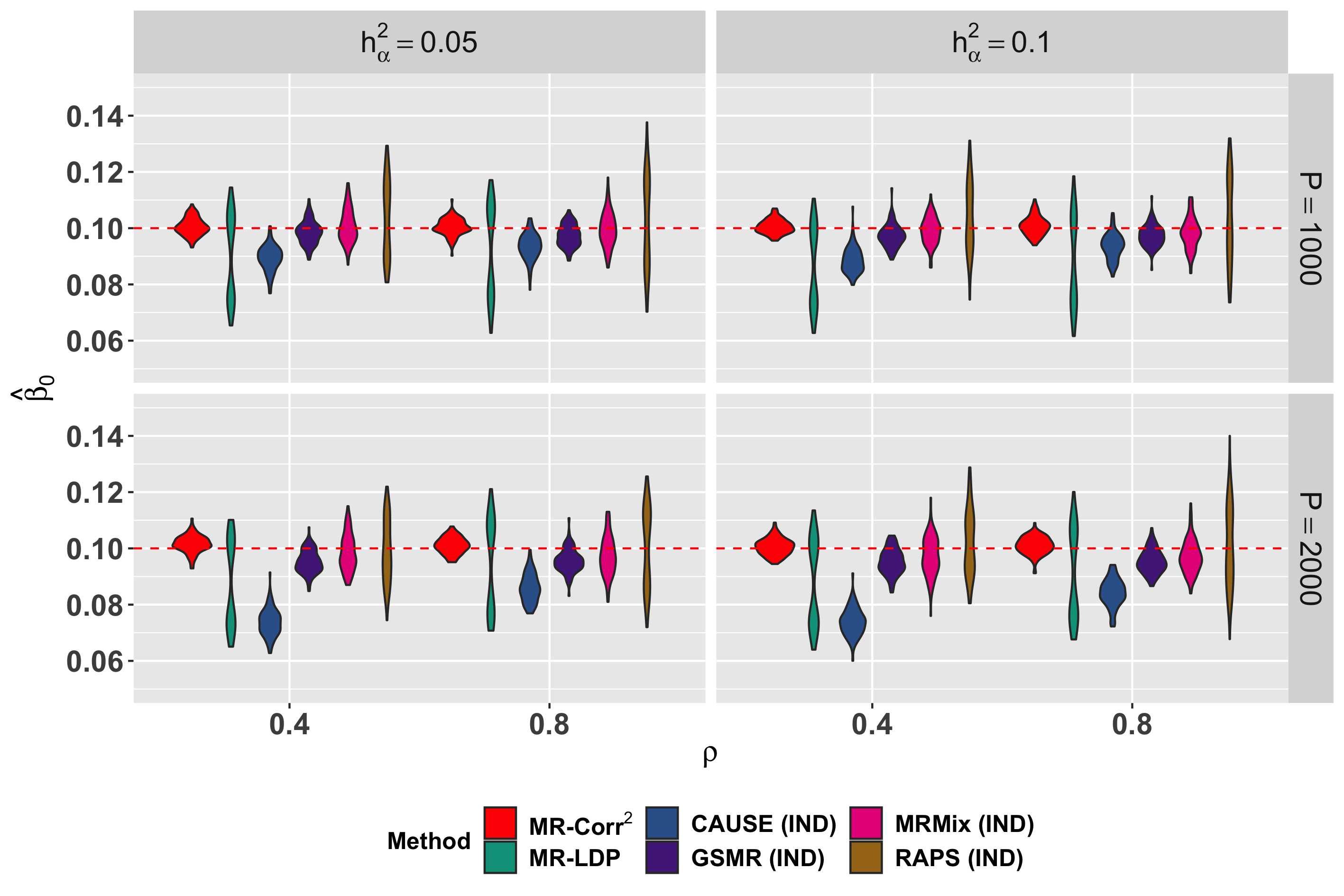
(d) Point estimate

Figure 4: Comparisons of type-I error and point estimate using correlated SNPs with $\rho_{\alpha\gamma}=0.2$. The number of replicates for type-I error is 1,000 and that for point estimates is 100. The top and bottom panels are corresponding to Scenario 1 and Scenario 2, respective. Note that we evaluate type-I error for CAUSE, GSMR, MRMix and RAPS using either all SNPs or independent SNPs.

5 Real Data Analysis

5.1 Real validations

Clearly, when there is no horizontal pleiotropy either correlated or independent, in other words, $\eta_{k}=0,\forall k$ , the proposed MR-Corr reduces to the classical MR methods that Eqn. (4) holds. Here, we used real datasets for height as both exposure and outcome to compare the estimates from MR-Corr and MR-Corr² with those from the other five alternative methods. As the exposure and outcome are the same complex traits, the causal effect $\beta_{0}$ can be taken as known, i.e., $\beta_{0}=1$. Since this type of analysis estimates the causal effects with known effect sizes under no horizontal pleiotropy, we make comparisons among the proposed and alternative methods to see the effectiveness of accounting for weak instrumental variants in LD.

In this validation study, we treated the summary statistics for height in UK Biobank [7] as the screening dataset, and chose the summary statistics for height in male and females in an European population-based study [33] as exposure and outcome, respectively. In the analysis, we first selected SNPs under different $p$-value threshold as instrumental variants. We next conducted SNP-clumping to obtain near-independent SNPs using PLINK [31] for MR-Corr, CAUSE, GSMR, MRMix and RAPS. For both MR-Corr² and MR-LDP, we conducted the analysis using all SNPs and used the genotype data from UK10K project [11] merged with 1000 Genome Project Phase 3 [10] as the reference dataset. The estimated causal effects with their corresponding standard errors using seven methods are summarized in Table 1. Clearly, 95% confidence intervals from MR-Corr, MR-Corr², MR-LDP, MRMix and RAPS cover the true $\beta_{0}$ but not for CAUSE and GSMR. Comparing to MR-Corr², MR-LDP and RAPS, the standard errors from MRMix are very large. On the other hand, using more correlated instrumental variants improves estimation efficiency for MR-Corr² and MR-LDP as both methods used SNPs in LD. This validation study demonstrates that the proposed methods perform well when there is no horizontal pleiotropy Eqn. (4). Moreover, methods using correlated SNPs, i.e., MR-Corr² and MR-LDP, are more statistically efficient.

Table 1: Results for height-height example. We chose 10 different $p$-value thresholds, $p_{\text{sel}}$, to select instrumental variants from $5\times 10^{-8}$ to $1\times 10^{-3}$, and reported the estimated causal effects with their corresponding standard errors for all six methods. Note that SNP clumping was performed to obtain independent SNPs for MR-Corr, CAUSE, GSMR, MRMix and RAPS.

$p_{\text{sel}}$	MR-Corr2	MR-LDP	MR-corr	CAUSE	GSMR	MRMix	RAPS
5e-08	1.010(0.019)	1.022(0.020)	1.012(0.026)	1.428(0.085)	0.789(0.021)	0.805(1.807)	1.015(0.034)
1e-07	1.011(0.020)	1.024(0.020)	1.015(0.029)	1.426(0.085)	0.784(0.021)	0.800(6.841)	1.019(0.035)
5e-07	1.007(0.020)	1.023(0.019)	1.010(0.028)	1.422(0.086)	0.738(0.020)	0.825(1.710)	1.017(0.036)
1e-06	1.005(0.018)	1.020(0.019)	1.005(0.028)	1.413(0.087)	0.730(0.019)	0.780(0.396)	1.008(0.036)
5e-06	1.001(0.019)	1.020(0.019)	1.011(0.029)	1.391(0.089)	0.709(0.019)	0.765(0.276)	1.018(0.039)
1e-05	1.001(0.019)	1.018(0.018)	0.996(0.030)	1.346(0.090)	0.694(0.019)	0.800(0.639)	1.004(0.039)
5e-05	0.996(0.018)	1.017(0.018)	0.992(0.031)	1.320(0.093)	0.649(0.018)	0.790(1.573)	0.997(0.042)
1e-04	0.997(0.019)	1.018(0.018)	0.985(0.028)	1.317(0.093)	0.627(0.017)	0.560(0.573)	0.991(0.043)
5e-04	0.989(0.018)	1.017(0.017)	0.982(0.032)	1.235(0.099)	0.562(0.017)	0.570(0.479)	1.006(0.053)

5.2 MR analysis for GWAS summary statistics

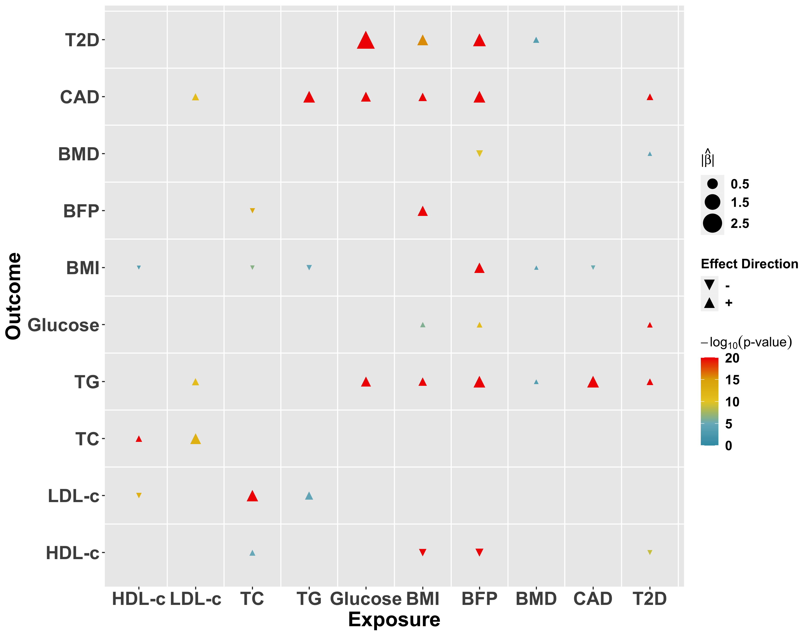
(a) MR-Corr²

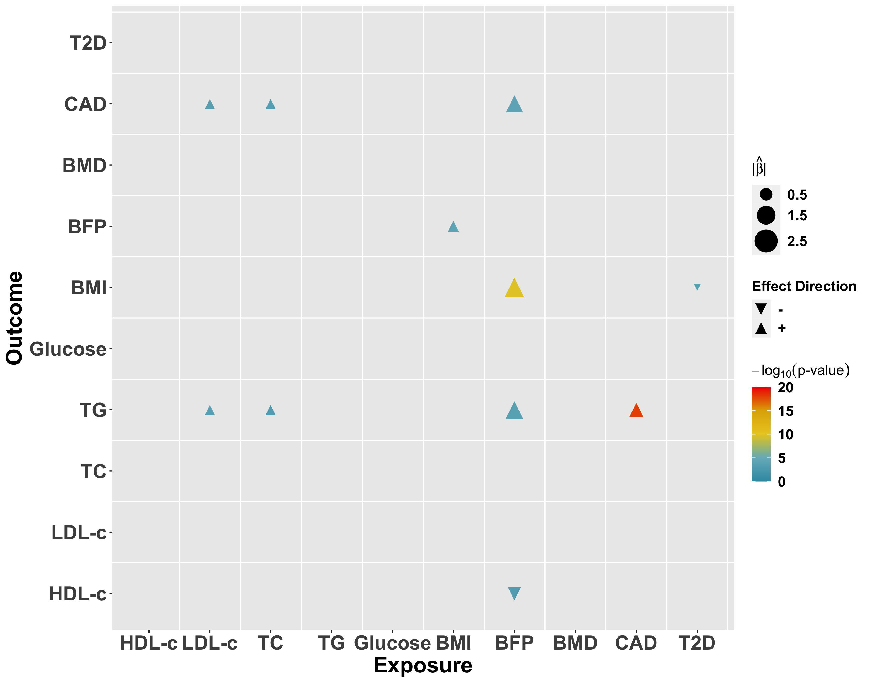
(b) CAUSE

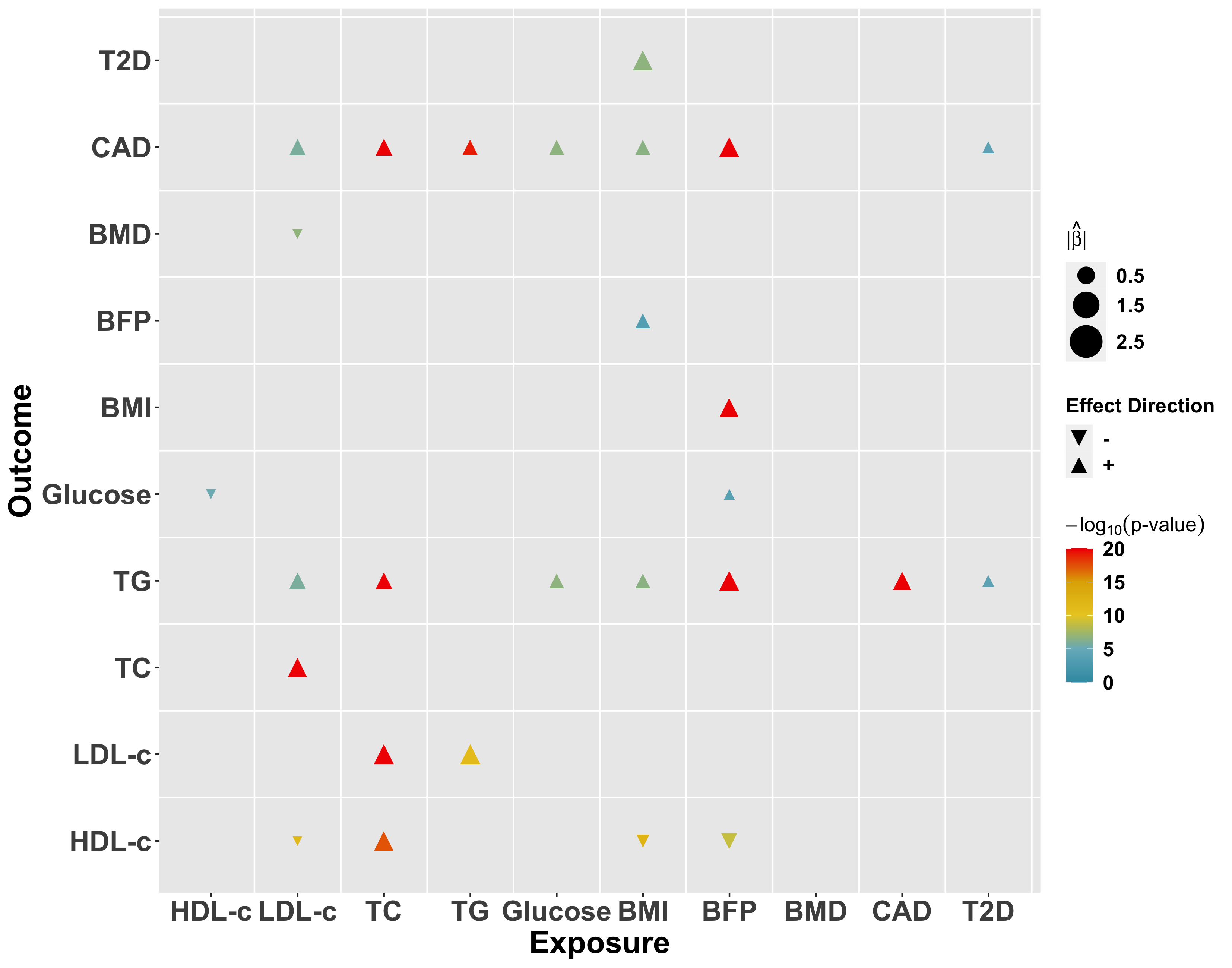
(c) MRMix

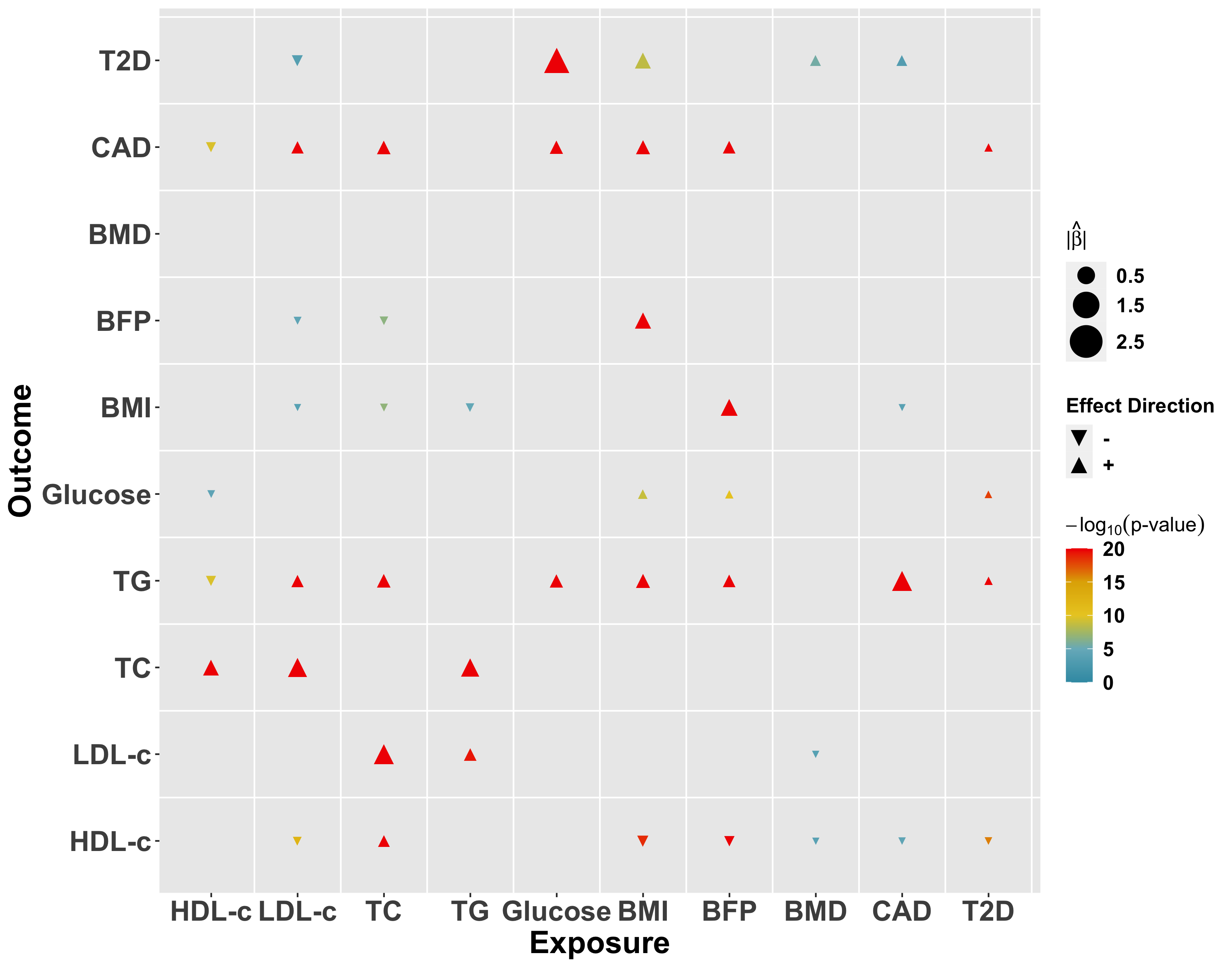
(d) GSMR

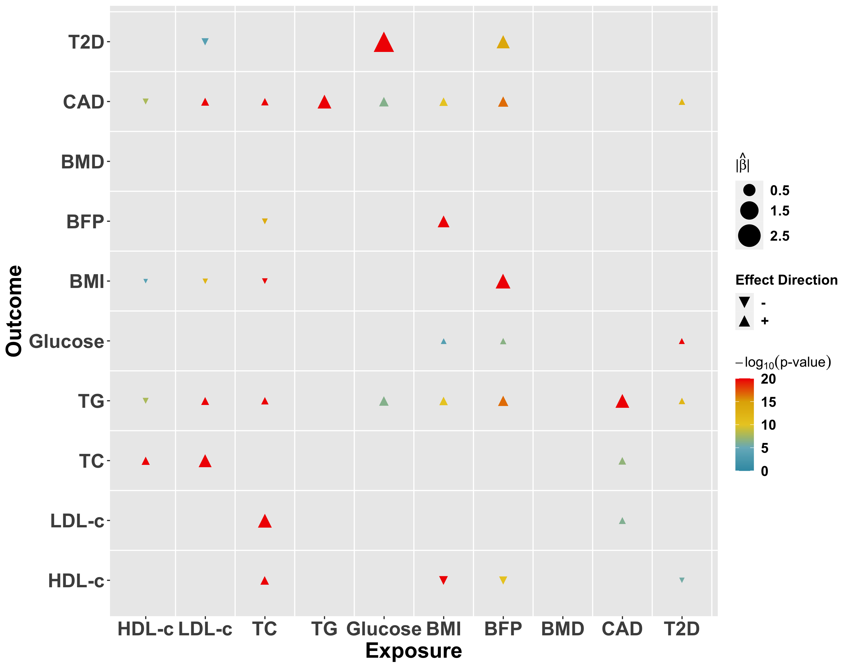
(e) MR-LDP

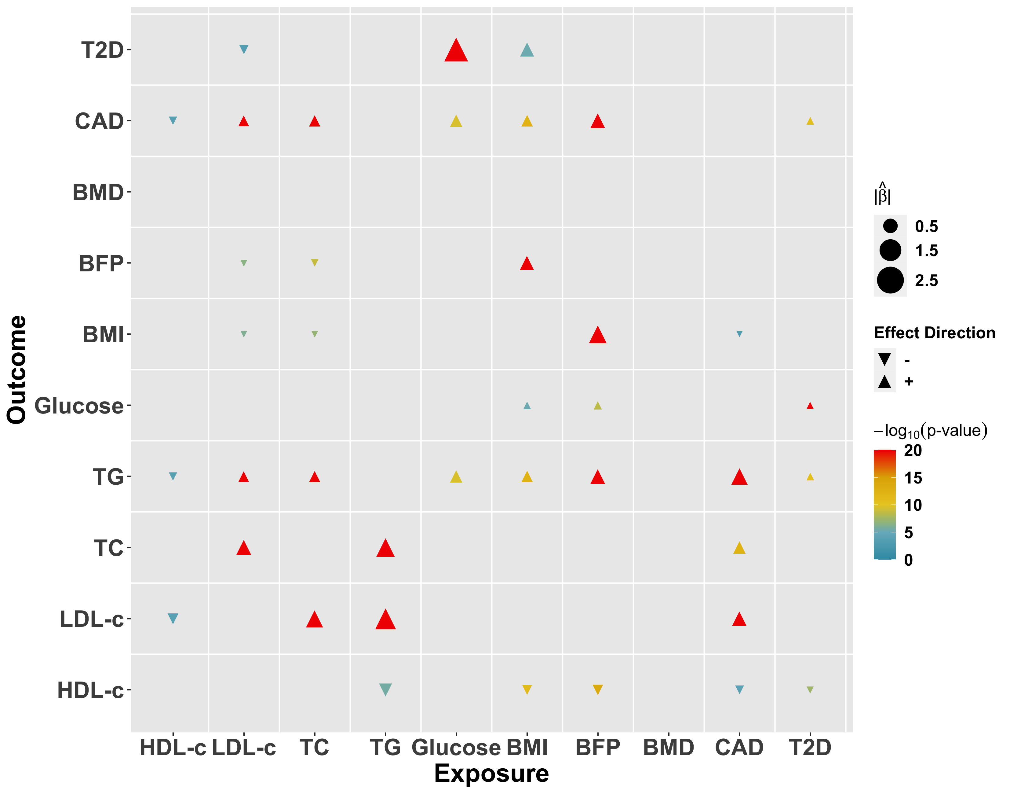
(f) RAPS

Figure 5: Estimated causal effects and their significance between exposure-outcome pairs among nine traits. In this plot, we show the magnitude ($|\hat{\beta}_{0}$) and direction (+ or -) of estimated causal effects together with their significance level ($-\log_{10}(p$-value)).

In the real data analysis, we applied six methods that are used in validation studies to analyze the causal effects between exposure-outcome pairs among two sets of traits. The first set contains ten traits, including low density lipoprotein cholesterol (LDL-c), high density lipoprotein cholesterol (HDL-c), total cholesterol (TC), triglycerides (TG), glucose, body fat percentage (BFP), total bone mineral density (BMD), body mass index (BMI), coronary artery disease (CAD), type 2 diabetes (T2D). The second set has five psychiatric disorders, including attention deficit hyperactivity disorder (ADHD), major depression disorder (MDD), bipolar disorder (BIP), schizophrenia (SCZ) and autism spectrum disorder (ASD). In the analysis using CAUSE, MRMix, GSMR and RAPS, we used $r^{2}=0.1$ to perform SNP clumping by CAUSE default. The results are shown in Figure 5 for MR-Corr², CAUSE, MRMix, GSMR, MR-LDP, and RAPS, respectively.

In the first set, since we conducted MR analysis for $10\times 9=90$ exposure-outcome pairs, we performed Bonferroni correction for significance level. In Figure 5, we identified 39, 11, 27, 45, 37 and 40 significant causal pairs using MR-Corr², CAUSE, MRMix, GSMR, MR-LDP, and RAPS, respectively. In details, many MR methods not correcting for CHP identified the significant causal effect of LDL-c on T2D [29]. But after correcting for CHP, MR-Corr² did not identify it significantly. One of the driving cause of T2D is insulin resistance [21]. And it is known that insulin resistance had profound effects on lipoproteins including LDL-c [16]. So the variants associated with insulin resistance could affect both T2D and LDL-c level, which is a case of CHP. As both BMI and BFP measure the level obesity, all six methods identified significant reverse causality between BMI and BFP with effect size close to 1, implying that the causal outcomes for BMI should be similar to those for BFP. As shown in Figure 5(a), both BMI and BFP are causally related to T2D based on our MR-Corr² test. However, all the other methods identified only one of them as the causal risk factor for T2D. It is known that both normal weight individuals with high BFP and overweight individuals with low BFP have higher risk for prediabetes or diabetes [20]. Therefore, only our method can uncover this combined effect of BMI and BFP on T2D. Other than T2D, we also consistently observe this combined effect on CAD as well as several metabolite levels. Besides BMI and BFP, we also identified two reverse causalities of T2D. One of them is T2D and glucose, which is expected because the most important characteristics of T2D is high fasting blood glucose [13]. The other novel reverse causality exits between T2D and BMD, which is consistent with the previous findings that BMD is increased in T2D patients [38].

Though the causal roles of LDL-c and TG on CAD are confirmed in different clinical trials [26], but it is not clear for the role of TC on CAD. After Bonferroni correction, MR-Corr² did not estimate the casual effect significantly between HDL-c and CAD but identified significantly by GSMR, MR-LDP and RAPS. Our result of MR-Corr² is consistent with those from clinical trials that use CETP inhibitor to raise the HDL-c level, but does not result in a lower rate of cardiovascular disease [25]. Recent studies show that patients with diabetes are at a substantially increased risk of dying from cardiovascular disease [15] while a recent trial shows that the beneficial effects of a sodium-glucose co-transporter 2 (SGLT2) inhibitor on prevention of hospitalization for heart failure therefore represent a significant clinical breakthrough [28]. The analysis using MR-Corr², MRMix, GSMR and MR-LDP confirms these established causal relationships.

In addition, we also observe several reverse causalities among lipid metabolites, which are TC-HDL-c, TC-LDL-c, and TG-LDL-c. These relationships are expected because they are naturally related with each other. For example, TC is a measure of LDL-c, HDL-c, and other lipid components, and LDL-c level can be calculated from TG [8].

For the second set of traits, we studied the causal relationships among psychiatric disorders. Since we conducted MR analysis for $5\times 4=20$ exposure-outcome pairs, we performed Bonferroni correction for significance level. It is well-known genetic correlations among psychiatric disorders are high, primarily due to the fact that common risk variants for psychiatric disorders are correlated significantly [1]. In Figure S4 (Supplementary), we identified 8, 0, 2, 7, 7 and 6 significant causal pairs using MR-Corr², CAUSE, MRMix, GSMR, MR-LDP, and RAPS, respectively. MR-Corr² identified four psychiatric disorders to be causally affected by MDD while RAPS and MR-LDP identify three, GSMR identifies two, and MRMix identified one among the four identified by MR-Corr². Meanwhile, MR-Corr², MR-LDP, GSMR and RAPS identified a significant positive causal effect of SCZ on ASD, BIP and MDD, and MR-Corr² , MR-LDP and GSMR identified a significant positive causal effect of ASD on ADHD. Table S2 in the Supplementary document shows the genetic correlations among these psychiatric disorders in [1]. A general pattern is that a significant correlation usually implies a causal relationship except for pairs in ADHD-BIP and ADHD-SCZ. These causal relationships may be attributable to the existence of a large number of medical comorbidities in psychiatric disorders [30]. The detailed results for causal inference and Venn plot for psychiatric disorders are shown in Table S3 and Figure S5 in the Supplementary document.

6 Discussion

In this study, we proposed MR-Corr² to account for CHP in the presence of correlated genetic variants. Mitigating the impact of CHP is important in MR/IV methods. We proposed a MLR strategy that first decomposes the direct effects into two parts, linear and orthogonal, then reparameterizes the relationship between $\bm{\gamma}$ and $\bm{\Gamma}$. In this way, the impact of CHP can be mitigated using model with variable selection, e.g., a spike-slab prior is used here. To incorporate correlated SNPs, we use an approximated distribution for summary statistics. Our validation studies which include both a real validation and simulations demonstrate that MR-Corr² controls type-I error at its nominal level and estimates the causal effects unbiasedly. In real data analysis, MR-Corr² did not identify the contradictory causal relationship between HDL-c and CAD, but identified multiple health outcomes, i.e., T2D, CAD, TG, and HDL-c, affected by obese risk factors (BMI and BFP) causally.

The proposed MLR strategy provides an effective and systematic framework to mitigate the impact of CHP in MR/IV methods. By connecting MLR strategy with CAUSE, it offers a unique perspective from correlated pleiotropy that is genetic variants affect unobserved confounders as shown in Figure 3(b). When there exist both correlated pleiotropy and IHP, an ideal model should allow linear relationship (4) deviates with IHP. Specifically, other than using Eqn. (11), we now can model an additional IHP, $\theta_{k}$, as

$$\Gamma_{k}=\left\{\begin{aligned} &\beta_{0}\gamma_{k}+\theta_{k},&&\widetilde{\alpha}_{k}=0\\ &\beta_{1}\gamma_{k}+\theta_{k}+\widetilde{\alpha}_{k},&&\widetilde{\alpha}_{k}\neq 0.\end{aligned}\right.$$ (20)

In this way, we will be able to handle both correlated pleiotropy as well as independent horizontal pleiotropy in the sense of CAUSE.

The other limitation of the proposed methods is that they do not account for sample overlap between SNP-exposure and SNP-outcome. For example, the samples are largely overlapped for lipid traits, i.e., HDL-c, LDL-c, TC and TC. Without correcting for these overlapped samples, the hypothesis test for causal effects between lipid traits tend to be inflated. We plan to address these challenges in future work.

References

- [1] V. Anttila, B. Bulik-Sullivan, H. K. Finucane, R. K. Walters, J. Bras, L. Duncan, V. Escott-Price, G. J. Falcone, P. Gormley, R. Malik, et al. Analysis of shared heritability in common disorders of the brain. Science, 360(6395), 2018.
- [2] J. Bowden, G. Davey Smith, and S. Burgess. Mendelian randomization with invalid instruments: effect estimation and bias detection through egger regression. International journal of epidemiology, 44(2):512–525, 2015.
- [3] J. Bowden, F. Del Greco M, C. Minelli, G. Davey Smith, N. Sheehan, and J. Thompson. A framework for the investigation of pleiotropy in two-sample summary data mendelian randomization. Statistics in medicine, 36(11):1783–1802, 2017.
- [4] J. Bowden, F. Del Greco M, C. Minelli, Q. Zhao, D. A. Lawlor, N. A. Sheehan, J. Thompson, and G. Davey Smith. Improving the accuracy of two-sample summary-data mendelian randomization: moving beyond the nome assumption. International journal of epidemiology, 48(3):728–742, 2019.
- [5] S. Burgess, A. Butterworth, and S. G. Thompson. Mendelian randomization analysis with multiple genetic variants using summarized data. Genetic epidemiology, 37(7):658–665, 2013.
- [6] S. Burgess and S. G. Thompson. Multivariable mendelian randomization: The use of pleiotropic genetic variants to estimate causal effects. American Journal of Epidemiology, 181(4):251–260, 2015.
- [7] C. Bycroft, C. Freeman, D. Petkova, G. Band, L. T. Elliott, K. Sharp, A. Motyer, D. Vukcevic, O. Delaneau, J. O’Connell, et al. The uk biobank resource with deep phenotyping and genomic data. Nature, 562(7726):203–209, 2018.
- [8] Y. Chen, X. Zhang, B. Pan, X. Jin, H. Yao, B. Chen, Y. Zou, J. Ge, and H. Chen. A modified formula for calculating low-density lipoprotein cholesterol values. Lipids in health and disease, 9(1):1–5, 2010.
- [9] Q. Cheng, Y. Yang, X. Shi, K.-F. Yeung, C. Yang, H. Peng, and J. Liu. Mr-ldp: a two-sample mendelian randomization for gwas summary statistics accounting for linkage disequilibrium and horizontal pleiotropy. NAR Genomics and Bioinformatics, 2(2):lqaa028, 2020.
- [10] . G. P. Consortium et al. A global reference for human genetic variation. Nature, 526(7571):68–74, 2015.
- [11] U. consortium et al. The uk10k project identifies rare variants in health and disease. Nature, 526(7571):82–90, 2015.
- [12] G. Davey Smith and S. Ebrahim. ‘mendelian randomization’: can genetic epidemiology contribute to understanding environmental determinants of disease? International journal of epidemiology, 32(1):1–22, 2003.
- [13] R. A. DeFronzo, E. Ferrannini, L. Groop, R. R. Henry, W. H. Herman, J. J. Holst, F. B. Hu, C. R. Kahn, I. Raz, G. I. Shulman, et al. Type 2 diabetes mellitus. Nature reviews Disease primers, 1(1):1–22, 2015.
- [14] V. Didelez and N. Sheehan. Mendelian randomization as an instrumental variable approach to causal inference. Statistical methods in medical research, 16(4):309–330, 2007.
- [15] D. H. Fitchett, J. A. Udell, and S. E. Inzucchi. Heart failure outcomes in clinical trials of glucose-lowering agents in patients with diabetes. European journal of heart failure, 19(1):43–53, 2017.
- [16] W. T. Garvey, S. Kwon, D. Zheng, S. Shaughnessy, P. Wallace, A. Hutto, K. Pugh, A. J. Jenkins, R. L. Klein, and Y. Liao. Effects of insulin resistance and type 2 diabetes on lipoprotein subclass particle size and concentration determined by nuclear magnetic resonance. Diabetes, 52(2):453–462, 2003.
- [17] F. D. Greco M, C. Minelli, N. A. Sheehan, and J. R. Thompson. Detecting pleiotropy in mendelian randomisation studies with summary data and a continuous outcome. Statistics in medicine, 34(21):2926–2940, 2015.
- [18] J. Huang, Y. Jiao, J. Liu, and C. Yang. Remi: Regression with marginal information and its application in genome-wide association studies. arXiv preprint arXiv:1805.01284, 2018.
- [19] H. Ishwaran, J. S. Rao, et al. Spike and slab variable selection: frequentist and bayesian strategies. The Annals of Statistics, 33(2):730–773, 2005.
- [20] A. Jo and A. G. Mainous III. Informational value of percent body fat with body mass index for the risk of abnormal blood glucose: a nationally representative cross-sectional study. BMJ open, 8(4), 2018.
- [21] A. M. Johnson and J. M. Olefsky. The origins and drivers of insulin resistance. Cell, 152(4):673–684, 2013.
- [22] M. Kanai, M. Akiyama, A. Takahashi, N. Matoba, Y. Momozawa, M. Ikeda, N. Iwata, S. Ikegawa, M. Hirata, K. Matsuda, et al. Genetic analysis of quantitative traits in the japanese population links cell types to complex human diseases. Nature genetics, 50(3):390–400, 2018.
- [23] H. Kang, A. Zhang, T. T. Cai, and D. S. Small. Instrumental variables estimation with some invalid instruments and its application to mendelian randomization. Journal of the American statistical Association, 111(513):132–144, 2016.
- [24] M. Kolesár, R. Chetty, J. Friedman, E. Glaeser, and G. W. Imbens. Identification and inference with many invalid instruments. Journal of Business & Economic Statistics, 33(4):474–484, 2015.
- [25] A. M. Lincoff, S. J. Nicholls, J. S. Riesmeyer, P. J. Barter, H. B. Brewer, K. A. Fox, C. M. Gibson, C. Granger, V. Menon, G. Montalescot, et al. Evacetrapib and cardiovascular outcomes in high-risk vascular disease. New England Journal of Medicine, 376(20):1933–1942, 2017.
- [26] N. A. Marston, R. P. Giugliano, K. Im, M. G. Silverman, M. L. O’Donoghue, S. D. Wiviott, B. A. Ference, and M. S. Sabatine. Association between triglyceride lowering and reduction of cardiovascular risk across multiple lipid-lowering therapeutic classes: A systematic review and meta-regression analysis of randomized controlled trials. Circulation, 140(16):1308–1317, 2019.
- [27] J. Morrison, N. Knoblauch, J. H. Marcus, M. Stephens, and X. He. Mendelian randomization accounting for correlated and uncorrelated pleiotropic effects using genome-wide summary statistics. Nature Genetics, pages 1–7, 2020.
- [28] M. E. Nassif and M. Kosiborod. A review of cardiovascular outcomes trials of glucose-lowering therapies and their effects on heart failure outcomes. The American Journal of Medicine, 132(10):S13–S20, 2019.
- [29] W. Pan, W. Sun, S. Yang, H. Zhuang, H. Jiang, H. Ju, D. Wang, and Y. Han. Ldl-c plays a causal role on t2dm: a mendelian randomization analysis. Aging (Albany NY), 12(3):2584, 2020.
- [30] O. Plana-Ripoll, C. B. Pedersen, Y. Holtz, M. E. Benros, S. Dalsgaard, P. De Jonge, C. C. Fan, L. Degenhardt, A. Ganna, A. N. Greve, et al. Exploring comorbidity within mental disorders among a danish national population. JAMA psychiatry, 76(3):259–270, 2019.
- [31] S. Purcell, B. Neale, K. Todd-Brown, L. Thomas, M. A. Ferreira, D. Bender, J. Maller, P. Sklar, P. I. De Bakker, M. J. Daly, et al. Plink: a tool set for whole-genome association and population-based linkage analyses. The American journal of human genetics, 81(3):559–575, 2007.
- [32] G. Qi and N. Chatterjee. Mendelian randomization analysis using mixture models for robust and efficient estimation of causal effects. Nature communications, 10(1):1–10, 2019.
- [33] J. C. Randall, T. W. Winkler, Z. Kutalik, S. I. Berndt, A. U. Jackson, K. L. Monda, T. O. Kilpeläinen, T. Esko, R. Mägi, S. Li, et al. Sex-stratified genome-wide association studies including 270,000 individuals show sexual dimorphism in genetic loci for anthropometric traits. PLoS Genet, 9(6):e1003500, 2013.
- [34] R. M. Sakia. The box-cox transformation technique: a review. Journal of the Royal Statistical Society: Series D (The Statistician), 41(2):169–178, 1992.
- [35] X. Shi, Y. Jiao, Y. Yang, C.-Y. Cheng, C. Yang, X. Lin, and J. Liu. Vimco: variational inference for multiple correlated outcomes in genome-wide association studies. Bioinformatics, 35(19):3693–3700, 2019.
- [36] E. J. T. Tchetgen, B. Sun, and S. Walter. The genius approach to robust mendelian randomization inference. arXiv preprint arXiv:1709.07779, 2017.
- [37] M. Verbanck, C.-y. Chen, B. Neale, and R. Do. Detection of widespread horizontal pleiotropy in causal relationships inferred from mendelian randomization between complex traits and diseases. Nature genetics, 50(5):693–698, 2018.
- [38] P. Vestergaard. Discrepancies in bone mineral density and fracture risk in patients with type 1 and type 2 diabetes—a meta-analysis. Osteoporosis international, 18(4):427–444, 2007.
- [39] Y. Yang, X. Shi, Y. Jiao, J. Huang, M. Chen, X. Zhou, L. Sun, X. Lin, C. Yang, and J. Liu. Comm-s2: a collaborative mixed model using summary statistics in transcriptome-wide association studies. Bioinformatics, 36(7):2009–2016, 2020.
- [40] J. Zhao, J. Ming, X. Hu, G. Chen, J. Liu, and C. Yang. Bayesian weighted mendelian randomization for causal inference based on summary statistics. Bioinformatics, 36(5):1501–1508, 2020.
- [41] Q. Zhao, J. Wang, J. Bowden, and D. S. Small. Statistical inference in two-sample summary-data mendelian randomization using robust adjusted profile score. arXiv preprint arXiv:1801.09652, 2018.
- [42] X. Zhu and M. Stephens. Bayesian large-scale multiple regression with summary statistics from genome-wide association studies. The annals of applied statistics, 11(3):1561, 2017.
- [43] Z. Zhu, Z. Zheng, F. Zhang, Y. Wu, M. Trzaskowski, R. Maier, M. R. Robinson, J. J. McGrath, P. M. Visscher, N. R. Wray, et al. Causal associations between risk factors and common diseases inferred from gwas summary data. Nature communications, 9(1):224, 2018.