The magic square of Lie groups:
the $2\times 2$ case

Abstract

A unified treatment of the $2\times 2$ analog of the Freudenthal-Tits magic square of Lie groups is given, providing an explicit representation in terms of matrix groups over composition algebras.

keywords: division algebras; magic squares; orthogonal groups; Clifford algebras

MSC: 22E46, 17A35, 15A66

1 Introduction

The Freudenthal–Tits magic square [1, 2] is a $4\times 4$ array of semisimple Lie algebras, whose rows and columns are labeled by composition algebras. It is magical not only because of its symmetry, but also because, in the row or column labeled by the octonions or the split octonions, the square produces four of the five exceptional Lie algebras: $\mathfrak{f}_{4}$, $\mathfrak{e}_{6}$, $\mathfrak{e}_{7}$ and $\mathfrak{e}_{8}$. Several constructions of the magic square are known [1, 2, 3, 4], all of which take a pair of composition algebras and produce a Lie algebra. They provide concise and elegant constructions of exceptional Lie algebras, and show how the exceptional Lie algebras are related to the octonions.

This paper forms part of an effort which aims to give a similarly concise and elegant construction for the exceptional Lie groups, by building a ‘magic square of Lie groups’; that is, we want a construction that takes two composition algebras and produces a Lie group, without the intermediate step of constructing the Lie algebra. In this paper, we construct the ‘$2\times 2$ magic square of Lie groups’. At the Lie algebra level, the ‘$2\times 2$ magic square’ proposed by Barton and Sudbery [4] is a simpler cousin of the Freudenthal–Tits magic square, so named because the $3\times 3$ matrices used in constructing the usual magic square are replaced by $2\times 2$ matrices. We emphasize that the labels ‘$2\times 2$’ and ‘$3\times 3$’ used throughout this paper refer to the size of the underlying matrices, and not to the magic squares themselves (which are $4\times 4$).

Unlike the original ‘$3\times 3$ magic square’, the $2\times 2$ magic square contains no exceptional Lie algebras. Instead, it consists of special orthogonal algebras with various signatures. It serves as a kind of test case for a similar analysis of the $3\times 3$ magic square, since it involves the noncommutativity of the quaternions and nonassociativity of the octonions without the further complexity of the exceptional Lie algebras. Moreover, it has an intriguing connection to string theory that makes it of interest in its own right: the first three rows give, in succession, the infinitesimal rotational, Lorentz, and conformal symmetries of the Minkowski spacetimes where the classical superstring can be defined. The octonionic column corresponds to 10-dimensional spacetime, where the superstring can also be quantized.

	$\mathbb{R}$	$\mathbb{C}$	$\mathbb{H}$	$\mathbb{O}$
$\mathbb{R}^{\prime}$	$\mathfrak{so}(3)$	$\mathfrak{su}(3)$	$\mathfrak{sp}(3)$	$\mathfrak{f}_{4}$
$\mathbb{C}^{\prime}$	$\mathfrak{sl}(3,\mathbb{R})$	$\mathfrak{sl}(3,\mathbb{C})$	$\mathfrak{a}_{5(-7)}$	$\mathfrak{e}_{6(-26)}$
$\mathbb{H}^{\prime}$	$\mathfrak{sp}(6,\mathbb{R})$	$\mathfrak{su}(3,3)$	$\mathfrak{d}_{6(-6)}$	$\mathfrak{e}_{7(-25)}$
$\mathbb{O}^{\prime}$	$\mathfrak{f}_{4(4)}$	$\mathfrak{e}_{6(2)}$	$\mathfrak{e}_{7(-5)}$	$\mathfrak{e}_{8(-24)}$

Table 1: The $3\times 3$ half-split magic square.

Our interest in this paper is in the ‘half-split’ magic square, with columns labeled by normed division algebras and rows by split composition algebras. To see the patterns we want to explore, first consider the half-split $3\times 3$ magic square shown in Table 1. Here, $\mathfrak{sp}(3)$ denotes the compact real form of $\mathfrak{c}_{3}$, whereas $\mathfrak{sp}(6,\mathbb{R})$ denotes the Lie algebra respecting the usual symplectic form on $\mathbb{R}^{6}$. A number in parentheses is the signature of the Killing form, which is the excess of plus signs (“boosts”) over minus signs (“rotations”) in the diagonalization of this form. As is well known, the Dynkin diagram and signature specify a real form completely.

Perhaps the most concise construction of the magic square is due to Vinberg. Given a pair of composition algebras $\mathbb{K}^{\prime}$ and $\mathbb{K}$, Vinberg’s construction [3] says the corresponding entry of the magic square will be

$$\mathfrak{v}_{3}(\mathbb{K}^{\prime},\mathbb{K})=\mathfrak{sa}_{3}(\mathbb{K}^{\prime}\otimes\mathbb{K})\oplus\mathfrak{der}(\mathbb{K}^{\prime})\oplus\mathfrak{der}(\mathbb{K}).$$ (1)

Here, $\mathfrak{sa}_{3}(\mathbb{K}^{\prime}\otimes\mathbb{K})$ denotes the set of traceless anti-Hermitian $3\times 3$ matrices, $\mathfrak{der}(\mathbb{K}^{\prime})$ and $\mathfrak{der}(\mathbb{K})$ are the Lie algebras of derivations on the composition algebras $\mathbb{K}^{\prime}$ and $\mathbb{K}$, and their sum is a Lie subalgebra. Since our focus is on the $2\times 2$ magic square in this paper, we will not need to describe the bracket on $\mathfrak{v}_{3}(\mathbb{K}^{\prime},\mathbb{K})$, which is given by a complicated formula that can be found in Barton and Sudbery [4].

Now make note of the pattern in the first two columns of the magic square. In what follows, $\mathbb{K}$ denotes $\mathbb{R}$ or $\mathbb{C}$, $\mathbb{K}^{n\times n}$ denotes the set of $n\times n$ matrices with entries in $\mathbb{K}$, and $X^{\dagger}=\overline{X}^{T}$, the conjugate transpose of the matrix $X$. We observe that:

• In the first row, $\mathfrak{so}(3)$ and $\mathfrak{su}(3)$ are both Lie algebras of traceless, anti-Hermitian matrices. If we define

  $$\mathfrak{su}(3,\mathbb{K})=\{X\in\mathbb{K}^{3\times 3}\,:\,X^{\dagger}=-X,\,\mathrm{tr\,}X=0\}.$$ (2)

  for $\mathbb{K}=\mathbb{R},\mathbb{C}$, then $\mathfrak{su}(3,\mathbb{R})$ is $\mathfrak{so}(3)$ and $\mathfrak{su}(3,\mathbb{C})$ is $\mathfrak{su}(3)$.

• In the second row, $\mathfrak{sl}(3,\mathbb{R})$ and $\mathfrak{sl}(3,\mathbb{C})$ are both Lie algebras of traceless matrices, that is, they are special cases of

  $$\mathfrak{sl}(3,\mathbb{K})=\{X\in\mathbb{K}^{3\times 3}\,:\,\mathrm{tr\,}X=0\}.$$ (3)

  for $\mathbb{K}=\mathbb{R},\mathbb{C}$.

We can carry our observations further if we note that $\mathfrak{su}(3,3)$ preserves an inner product on $\mathbb{C}^{6}$ that, in a suitable basis, bears a striking resemblance to a symplectic form:

$$\omega(x,y)=x^{\dagger}\left(\begin{matrix}0&1\\ -1&0\end{matrix}\right)y,$$ (4)

where we regard $x,y\in\mathbb{C}^{6}$ as column vectors. The only difference between $\omega$ and the usual symplectic structure is that $\omega$ is conjugate linear in its first slot. Thus, we see that:

• In the third row, $\mathfrak{sp}(6,\mathbb{R})$ and $\mathfrak{su}(3,3)$ are both Lie algebras of the form

  $$\mathfrak{sp}(6,\mathbb{K})=\{X\in\mathbb{K}^{6\times 6}\,:\,X^{\dagger}J+JX=0,\,\mathrm{tr\,}X=0\}$$ (5)

  for $\mathbb{K}=\mathbb{R},\mathbb{C}$, where $J$ is the $6\times 6$ matrix with block decomposition $J=\left(\begin{matrix}0&1\\ -1&0\end{matrix}\right)$.

Barton and Sudbery showed how to extend these patterns across the first three rows by giving definitions of Lie algebras $\mathfrak{su}(n,\mathbb{K})$, $\mathfrak{sl}(n,\mathbb{K})$ and $\mathfrak{sp}(2n,\mathbb{K})$ that work when $\mathbb{K}$ is any normed division algebra, provided $n\leq 3$, and for any $n$ when $\mathbb{K}$ is associative.

	$\mathbb{R}$	$\mathbb{C}$	$\mathbb{H}$	$\mathbb{O}$
$\mathbb{R}^{\prime}$	$\mathfrak{su}(3,\mathbb{R})$	$\mathfrak{su}(3,\mathbb{C})$	$\mathfrak{su}(3,\mathbb{H})$	$\mathfrak{su}(3,\mathbb{O})$
$\mathbb{C}^{\prime}$	$\mathfrak{sl}(3,\mathbb{R})$	$\mathfrak{sl}(3,\mathbb{C})$	$\mathfrak{sl}(3,\mathbb{H})$	$\mathfrak{sl}(3,\mathbb{O})$
$\mathbb{H}^{\prime}$	$\mathfrak{sp}(6,\mathbb{R})$	$\mathfrak{sp}(6,\mathbb{C})$	$\mathfrak{sp}(6,\mathbb{H})$	$\mathfrak{sp}(6,\mathbb{O})$

Table 2: The $3\times 3$ magic square, first three rows according to Barton and Sudbery.

When $n=3$, the above algebras reproduce the first three rows of the $3\times 3$ magic square, as shown in Table 2. Of particular interest, the exceptional Lie algebras are:

$$\mathfrak{su}(3,\mathbb{O})=\mathfrak{f}_{4},\quad\mathfrak{sl}(3,\mathbb{O})=\mathfrak{e}_{6(-26)},\quad\mathfrak{sp}(6,\mathbb{O})=\mathfrak{e}_{7(-25)}.$$ (6)

On the other hand, when $n=2$, $\mathfrak{su}(2,\mathbb{K})$, $\mathfrak{sl}(2,\mathbb{K})$ and $\mathfrak{sp}(4,\mathbb{K})$ turn out to be orthogonal Lie algebras, namely

$$\mathfrak{su}(2,\mathbb{K})=\mathfrak{so}(\mathbb{R}^{\prime}\oplus\mathbb{K}),\quad\mathfrak{sl}(2,\mathbb{K})=\mathfrak{so}(\mathbb{C}^{\prime}\oplus\mathbb{K}),\quad\mathfrak{sp}(4,\mathbb{K})=\mathfrak{so}(\mathbb{H}^{\prime}\oplus\mathbb{K}),$$ (7)

where the direct sums above are orthogonal direct sums. This leads Barton and Sudbery to take the half-split $2\times 2$ magic square to be the square with entry $\mathfrak{so}(\mathbb{K}^{\prime}\oplus\mathbb{K})$ for any split composition algebra $\mathbb{K}^{\prime}$ and normed division algebra $\mathbb{K}$, as shown in Table 3. The given signatures follow from adding the signatures of $\mathbb{K}^{\prime}$ and $\mathbb{K}$ in the orthogonal direct sum. We will delve further into the properties of composition algebras later.

	$\mathbb{R}$	$\mathbb{C}$	$\mathbb{H}$	$\mathbb{O}$
$\mathbb{R}^{\prime}$	$\mathfrak{so}(2)$	$\mathfrak{so}(3)$	$\mathfrak{so}(5)$	$\mathfrak{so}(9)$
$\mathbb{C}^{\prime}$	$\mathfrak{so}(2,1)$	$\mathfrak{so}(3,1)$	$\mathfrak{so}(5,1)$	$\mathfrak{so}(9,1)$
$\mathbb{H}^{\prime}$	$\mathfrak{so}(3,2)$	$\mathfrak{so}(4,2)$	$\mathfrak{so}(6,2)$	$\mathfrak{so}(10,2)$
$\mathbb{O}^{\prime}$	$\mathfrak{so}(5,4)$	$\mathfrak{so}(6,4)$	$\mathfrak{so}(8,4)$	$\mathfrak{so}(12,4)$

Table 3: The $2\times 2$ magic square.

Despite its different appearance, this $2\times 2$ magic square really is a cousin of the $3\times 3$ magic square. Barton and Sudbery prove that each entry of this magic square is given by a construction similar to Vinberg’s, namely

$$\mathfrak{v}_{2}(\mathbb{K}^{\prime},\mathbb{K})=\mathfrak{sa}_{2}(\mathbb{K}^{\prime}\otimes\mathbb{K})\oplus\mathfrak{so}(\mathrm{Im}\,\mathbb{K}^{\prime})\oplus\mathfrak{so}(\mathrm{Im}\,\mathbb{K}).$$ (8)

Now, $\mathfrak{sa}_{2}(\mathbb{K}^{\prime}\otimes\mathbb{K})$ denotes the set of traceless, anti-Hermitian $2\times 2$ matrices over $\mathbb{K}^{\prime}\otimes\mathbb{K}$, while $\mathrm{Im}\,\mathbb{K}^{\prime}$ and $\mathrm{Im}\,\mathbb{K}$ denote the ‘imaginary parts’ of $\mathbb{K}^{\prime}$ and $\mathbb{K}$, respectively. In contrast to Vinberg’s construction of the $3\times 3$ magic square, the algebras of derivations have been replaced with the orthogonal algebras $\mathfrak{so}(\mathrm{Im}\,\mathbb{K}^{\prime})$ and $\mathfrak{so}(\mathrm{Im}\,\mathbb{K})$. However, just as for the $3\times 3$ magic square, the first three rows can be expressed in terms of (generalized) unitary, linear, and symplectic algebras, as shown in Table 4; compare Table 2.

	$\mathbb{R}$	$\mathbb{C}$	$\mathbb{H}$	$\mathbb{O}$
$\mathbb{R}^{\prime}$	$\mathfrak{su}(2,\mathbb{R})$	$\mathfrak{su}(2,\mathbb{C})$	$\mathfrak{su}(2,\mathbb{H})$	$\mathfrak{su}(2,\mathbb{O})$
$\mathbb{C}^{\prime}$	$\mathfrak{sl}(2,\mathbb{R})$	$\mathfrak{sl}(2,\mathbb{C})$	$\mathfrak{sl}(2,\mathbb{H})$	$\mathfrak{sl}(2,\mathbb{O})$
$\mathbb{H}^{\prime}$	$\mathfrak{sp}(4,\mathbb{R})$	$\mathfrak{sp}(4,\mathbb{C})$	$\mathfrak{sp}(4,\mathbb{H})$	$\mathfrak{sp}(4,\mathbb{O})$

Table 4: The $2\times 2$ magic square, first three rows.

Of particular interest, the octonionic column becomes:

$$\mathfrak{su}(2,\mathbb{O})=\mathfrak{so}(9),\quad\mathfrak{sl}(2,\mathbb{O})=\mathfrak{so}(9,1),\quad\mathfrak{sp}(4,\mathbb{O})=\mathfrak{so}(10,2).$$ (9)

These are, respectively, the Lie algebras of infinitesimal rotations, Lorentz transformations, and conformal transformations for Minkowski spacetime $\mathbb{R}^{9,1}$, which is of precisely the dimension where string theory can be quantized. This intriguing connection to the octonions is not a coincidence [5, 6, 7], but is far from fully understood.

Dray, Manogue and their collaborators have worked steadily to lift Barton and Sudbery’s construction of the Lie algebras $\mathfrak{su}(n,\mathbb{O})$, $\mathfrak{sl}(n,\mathbb{O})$ and $\mathfrak{sp}(2n,\mathbb{O})$ to the group level. In the case $n=2$, Manogue and Schray [8] gave an explicit octonionic representation of the Lorentz group $\mathrm{SO}(9,1)$ in 10 spacetime dimensions, and later Manogue and Dray [9, 10] outlined the implications of this mathematical description for the description of fundamental particles. In brief, Manogue and Schray constructed a group that deserves to be called $\mathrm{SL}(2,\mathbb{O})$ that was the double cover of (the identity component of) $\mathrm{SO}(9,1)$, that is:

$$\mathrm{SL}(2,\mathbb{O})\equiv\mathrm{SO}(9,1).$$ (10)

Here we use the symbol “$\equiv$” to mean “isomorphic up to cover”—that is, we will write $G\equiv H$ to mean the Lie groups $G$ and $H$ have the same Lie algebra. Moving one step up in the magic square, if we define $\mathrm{SU}(2,\mathbb{O})$ to be the maximal compact subgroup of $\mathrm{SL}(2,\mathbb{O})$, we also get:

$$\mathrm{SU}(2,\mathbb{O})\equiv\mathrm{SO}(9).$$ (11)

Because all other division algebras are subalgebras of the octonions, these two constructions fully capture the first two rows of the $2\times 2$ magic square of Lie groups shown in Table 5.

	$\mathbb{R}$	$\mathbb{C}$	$\mathbb{H}$	$\mathbb{O}$
$\mathbb{R}^{\prime}$	$\mathrm{SU}(2,\mathbb{R})\equiv\mathrm{SO}(2)$	$\mathrm{SU}(2,\mathbb{C})\equiv\mathrm{SO}(3)$	$\mathrm{SU}(2,\mathbb{H})\equiv\mathrm{SO}(5)$	$\mathrm{SU}(2,\mathbb{O})\equiv\mathrm{SO}(9)$
$\mathbb{C}^{\prime}$	$\mathrm{SL}(2,\mathbb{R})\equiv\mathrm{SO}(2,1)$	$\mathrm{SL}(2,\mathbb{C})\equiv\mathrm{SO}(3,1)$	$\mathrm{SL}(2,\mathbb{H})\equiv\mathrm{SO}(5,1)$	$\mathrm{SL}(2,\mathbb{O})\equiv\mathrm{SO}(9,1)$
$\mathbb{H}^{\prime}$	$\mathrm{Sp}(4,\mathbb{R})\equiv\mathrm{SO}(3,2)$	$\mathrm{SU}(2,2)\equiv\mathrm{SO}(4,2)$	$\mathrm{SO}(6,2)$	$\mathrm{SO}(10,2)$
$\mathbb{O}^{\prime}$	$\mathrm{SO}(5,4)$	$\mathrm{SO}(6,4)$	$\mathrm{SO}(8,4)$	$\mathrm{SO}(12,4)$

Table 5: The $2\times 2$ magic square of Lie groups.

More recently, Dray and Manogue [11, 12] have extended these results to the exceptional Lie group $\mathrm{E}_{6}$, using the framework described in more detail by Wangberg and Dray [13, 14] and in Wangberg’s thesis [15]. All of these results rely on the description of certain groups using matrices over division algebras. Just as $\mathrm{SL}(2,\mathbb{O})$ appears in the second row and last column of the $2\times 2$ magic square of Lie groups, $\mathrm{E}_{6}$ appears in the corresponding spot of the $3\times 3$ magic square. Using $\mathrm{SL}(2,\mathbb{O})$ to bootstrap the process, Dray, Manogue and Wangberg define a group that deserves to be called $\mathrm{SL}(3,\mathbb{O})$ and prove that:

$$\mathrm{SL}(3,\mathbb{O})\equiv\mathrm{E}_{6(-26)}$$ (12)

where, again, we take the symbol $\equiv$ to mean “isomorphic up to cover”. As before, if we take $\mathrm{SU}(3,\mathbb{O})$ to be the maximal compact subgroup of $\mathrm{SL}(3,\mathbb{O})$, we immediately obtain:

$$\mathrm{SU}(3,\mathbb{O})\equiv\mathrm{F}_{4}.$$ (13)

Once again, because all other normed division algebras are subalgebras of the octonions, we obtain the first two rows of the $3\times 3$ magic square of Lie groups, as shown in Table 6.

	$\mathbb{R}$	$\mathbb{C}$	$\mathbb{H}$	$\mathbb{O}$
$\mathbb{R}^{\prime}$	$\mathrm{SU}(3,\mathbb{R})$	$\mathrm{SU}(3,\mathbb{C})$	$\mathrm{SU}(3,\mathbb{H})\equiv\mathrm{C}_{3}$	$\mathrm{SU}(3,\mathbb{O})\equiv\mathrm{F}_{4}$
$\mathbb{C}^{\prime}$	$\mathrm{SL}(3,\mathbb{R})$	$\mathrm{SL}(3,\mathbb{C})$	$\mathrm{SL}(3,\mathbb{H})\equiv\mathrm{A}_{5(-7)}$	$\mathrm{SL}(3,\mathbb{O})\equiv\mathrm{E}_{6(-26)}$
$\mathbb{H}^{\prime}$	$\mathrm{Sp}(6,\mathbb{R})\equiv\mathrm{C}_{3(3)}$	$\mathrm{SU}(3,3)$	$\mathrm{D}_{6(-6)}$	$\mathrm{E}_{7(-25)}$
$\mathbb{O}^{\prime}$	$\mathrm{F}_{4(4)}$	$\mathrm{E}_{6(2)}$	$\mathrm{E}_{7(-5)}$	$\mathrm{E}_{8(-24)}$

Table 6: The $3\times 3$ magic square of Lie groups.

The ultimate goal of this project is to extend the above descriptions from the first two rows of the magic squares to the remaining two rows, culminating in new constructions of the exceptional Lie groups $\mathrm{E}_{7}$ and $\mathrm{E}_{8}$. An additional step in this direction was recently taken by Dray, Manogue, and Wilson [16], who showed that

$$\mathrm{Sp}(6,\mathbb{O})\equiv\mathrm{E}_{7(-25)}$$ (14)

and along the way also that

$$\mathrm{Sp}(4,\mathbb{O})\equiv\mathrm{SO}(10,2),$$ (15)

thus completing the interpretation of the third row in both Lie group magic squares; Wilson [17] has also recently given a quaternionic construction of $\mathrm{E}_{7}$. But what about the fourth row?

In this paper, we take a different approach, and develop some tools for working with the entire $2\times 2$ magic square at once. At the Lie algebra level, recall that this magic square consists of the orthogonal algebras $\mathfrak{so}(\mathbb{K}\oplus\mathbb{K}^{\prime})$, where “$\oplus$” denotes the orthogonal direct sum. We will show how to use composition algebras to talk about the corresponding Lie groups, in two different ways.

First, using composition algebras, we will construct a module of the Clifford algebra $\mathrm{C}\ell(\mathbb{K}\oplus\mathbb{K}^{\prime})$ on the space of $4\times 4$ matrices with entries in $\mathbb{K}^{\prime}\otimes\mathbb{K}$. In the standard way, this gives a representation of $\mathrm{Spin}(\mathbb{K}\oplus\mathbb{K}^{\prime})$ on $(\mathbb{K}^{\prime}\otimes\mathbb{K})^{4\times 4}$. Identifying a certain subspace of the $4\times 4$ matrices, $(\mathbb{K}^{\prime}\otimes\mathbb{K})^{4\times 4}$, with $\mathbb{K}\oplus\mathbb{K}^{\prime}$, this representation will restrict to the usual representation of $\mathrm{Spin}(\mathbb{K}\oplus\mathbb{K}^{\prime})$ on $\mathbb{K}\oplus\mathbb{K}^{\prime}$.

We will then show that each group in the $2\times 2$ magic square can be written in the form $\mathrm{SU}(2,\mathbb{K}^{\prime}\otimes\mathbb{K})$. Kincaid and Dray [18, 19] took the first step in providing a composition algebra description of the third row of the magic squares by showing that $\mathrm{SO}(4,2)\equiv\mathrm{SU}(2,\mathbb{H}^{\prime}\otimes\mathbb{C})$. We extend their work by showing that $\mathrm{Spin}(\mathbb{K}\oplus\mathbb{K}^{\prime})$ acts on $\mathbb{K}\oplus\mathbb{K}^{\prime}$ just as $\mathrm{SU}(2,\mathbb{C})$ acts on the space of $2\times 2$ Hermitian matrices. We therefore rechristen $\mathrm{Spin}(\mathbb{K}\oplus\mathbb{K}^{\prime})$ as $\mathrm{SU}(2,\mathbb{K}^{\prime}\otimes\mathbb{K})$ when working with this representation.

2 Composition Algebras

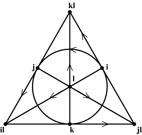
Figure 1: A graphical representation of the octonionic multiplication table.

	$i$	$j$	$k$	$k\ell$	$j\ell$	$i\ell$	$\ell$
$i$	$-1$	$k$	$-j$	$j\ell$	$-k\ell$	$\ell$	$i\ell$
$j$	$-k$	$-1$	$i$	$-i\ell$	$\ell$	$k\ell$	$j\ell$
$k$	$j$	$-i$	$-1$	$-\ell$	$i\ell$	$-j\ell$	$k\ell$
$k\ell$	$-j\ell$	$i\ell$	$\ell$	$-1$	$i$	$-j$	$-k$
$j\ell$	$k\ell$	$\ell$	$-i\ell$	$-i$	$-1$	$k$	$-j$
$i\ell$	$\ell$	$-k\ell$	$j\ell$	$j$	$-k$	$-1$	$-i$
$\ell$	$-i\ell$	$-j\ell$	$-k\ell$	$k$	$j$	$i$	$-1$

Table 7: The octonionic multiplication table.

	$I$	$J$	$K$	$KL$	$JL$	$IL$	$L$
$I$	$-1$	$K$	$-J$	$JL$	$-KL$	$-L$	$IL$
$J$	$-K$	$-1$	$I$	$-IL$	$-L$	$KL$	$JL$
$K$	$J$	$-I$	$-1$	$-L$	$IL$	$-JL$	$KL$
$KL$	$-JL$	$IL$	$L$	$1$	$-I$	$J$	$K$
$JL$	$KL$	$L$	$-IL$	$I$	$1$	$-K$	$J$
$IL$	$L$	$-KL$	$JL$	$-J$	$K$	$1$	$I$
$L$	$-IL$	$-JL$	$-KL$	$-K$	$-J$	$-I$	$1$

Table 8: The split octonionic multiplication table.

A composition algebra $\mathbb{K}$ is a nonassociative real algebra with a multiplicative unit 1 equipped with a nondegenerate quadratic form $Q$ satisfying the composition property:

$$Q(xy)=Q(x)Q(y),\quad x,y\in\mathbb{K}.$$ (16)

A composition algebra for which $Q$ is positive definite is called a normed division algebra. On the other hand, when $Q$ is indefinite, $\mathbb{K}$ is called a split composition algebra. In the latter case, it was shown by Albert [20] that the quadratic form $Q$ must be ‘split’. Recall that the signature of a quadratic form is the excess of plus signs over minus signs in its diagonalization. A nondegenerate quadratic form on a real vector space is split if its signature is as close to 0 as possible: 0 for an even dimensional space, and $\pm 1$ for an odd dimensional space.

By a theorem of Hurwitz [21], there are exactly four normed division algebras: the real numbers $\mathbb{R}$, the complex numbers $\mathbb{C}$, the quaternions $\mathbb{H}$, and the octonions $\mathbb{O}$. Similarly, there are exactly four split composition algebras: the real numbers $\mathbb{R}^{\prime}=\mathbb{R}$, the split complex numbers $\mathbb{C}^{\prime}$, the split quaternions $\mathbb{H}^{\prime}$, and the split octonions $\mathbb{O}^{\prime}$. In either case, these algebras have dimensions 1, 2, 4, and 8, respectively.

Let us sketch the construction of the normed division algebras and their split cousins. Because the octonions and the split octonions contain all the other composition algebras as subalgebras, we will invert the usual order and construct them first.

The octonions $\mathbb{O}$ are the real algebra spanned by the multiplicative unit 1 and seven square roots of $-1$:

$$\mathbb{O}=\mathrm{span}\{1,i,j,k,k\ell,j\ell,i\ell,\ell\}.$$ (17)

The basis elements besides $1$ are called imaginary units. The products of these imaginary units are best encapsulated in a figure known as the Fano plane, equipped with oriented edges, as shown in Figure 1. Here, the product of any two elements is equal to the third element on the same edge, with a minus sign if multiplying against orientation. For instance:

$$j(i\ell)=k\ell=-(i\ell)j.$$ (18)

As we alluded to above, the square of any imaginary unit is $-1$. These rules suffice to multiply any pair of octonions; the imaginary units $k\ell,j\ell,i\ell$ are precisely the products suggested by their names. The full multiplication table is given in Table 7.

All other normed division algebras are subalgebras of $\mathbb{O}$. The real numbers $\mathbb{R}$ are the subalgebra spanned by $1$, the complex numbers $\mathbb{C}$ are the subalgebra spanned by $\{1,i\}$, and the quaternions $\mathbb{H}$ are the subalgebra spanned by $\{1,i,j,k\}$. Of course, there are many other copies of $\mathbb{C}$ and $\mathbb{H}$ in $\mathbb{O}$. This construction can be reversed, using the Cayley–Dickson process [22]; as vector spaces, we have

$$\mathbb{C}=\mathbb{R}\oplus\mathbb{R}i,\quad\mathbb{H}=\mathbb{C}\oplus\mathbb{C}j,\quad\mathbb{O}=\mathbb{H}\oplus\mathbb{H}\ell.$$ (19)

Conjugation is the linear map on $\mathbb{O}$ which fixes 1 and sends every imaginary unit to its negative. It restricts to an operation on $\mathbb{R}$, $\mathbb{C}$ and $\mathbb{H}$, also called conjugation, which is trivial on $\mathbb{R}$, and coincides with the usual conjugation on $\mathbb{C}$ and $\mathbb{H}$. For an arbitrary octonion $x\in\mathbb{O}$, we write its conjugate as $\overline{x}$. We define the real and imaginary part of $x$ with the usual formulas,

$$\mathrm{Re}\,(x)=\frac{x+\overline{x}}{2},\quad\mathrm{Im}\,(x)=\frac{x-\overline{x}}{2},$$ (20)

and we say that $x$ is real or imaginary if it is equal to its real or imaginary part, respectively. The set of all imaginary octonions is denoted $\mathrm{Im}\,\mathbb{O}$. Our notation and terminology for the other normed division algebras is similar.

We can show that for a pair of octonions $x,y\in\mathbb{O}$, conjugation satisfies $\overline{xy}=\overline{y}\>\overline{x}$. The quadratic form on $\mathbb{O}$ is defined by:

$$Q(x)=x\overline{x}=\overline{x}x.$$ (21)

We will also write $Q(x)$ as $|x|^{2}$. Polarizing, we see the quadratic form comes from the inner product:

$$(x,y)=\mathrm{Re}\,(x\overline{y})=\mathrm{Re}\,(\overline{x}y).$$ (22)

Moreover, a straightforward calculation shows that $1$ and the imaginary units are orthonormal with respect to this inner product. Explicitly, if

$$a=a_{1}1+a_{2}i+a_{3}j+a_{4}k+a_{5}k\ell+a_{6}j\ell+a_{7}i\ell+a_{8}\ell$$ (23)

we have

$$|a|^{2}=a_{1}^{2}+a_{2}^{2}+a_{3}^{2}+a_{4}^{2}+a_{5}^{2}+a_{6}^{2}+a_{7}^{2}+a_{8}^{2},$$ (24)

so the quadratic form is positive definite. Finally, it follows from the definition that the quadratic form satisfies the composition property:

$$|xy|^{2}=|x|^{2}|y|^{2},\quad x,y\in\mathbb{O}.$$ (25)

Thus, $\mathbb{O}$ is a normed division algebra, as promised. The quadratic form and inner product restrict to the other normed division algebras, and we use the same notation.

The split octonions $\mathbb{O}^{\prime}$ are the real algebra spanned by the multiplicative unit 1 and three square roots of $-1$, and four square roots of $+1$:

$$\mathbb{O}^{\prime}=\mathrm{span}\{1,I,J,K,KL,JL,IL,L\}.$$ (26)

The basis elements besides $1$ are again called imaginary units. The products of these imaginary units are given in Table 8.

All other split composition algebras are subalgebras of $\mathbb{O}^{\prime}$. The split real numbers $\mathbb{R}^{\prime}$ are the subalgebra spanned by $1$, the split complex numbers $\mathbb{C}^{\prime}$ are the subalgebra spanned by $\{1,L\}$, and the split quaternions $\mathbb{H}^{\prime}$ are the subalgebra spanned by $\{1,L,K,KL\}$. Of course, there are many other copies of $\mathbb{C}^{\prime}$ and $\mathbb{H}^{\prime}$ in $\mathbb{O}^{\prime}$. Finally, the split real numbers, split complex numbers and split quaternions have more familiar forms, namely

$$\mathbb{R}^{\prime}=\mathbb{R},\quad\mathbb{C}^{\prime}\cong\mathbb{R}\oplus\mathbb{R},\quad\mathbb{H}^{\prime}\cong\mathbb{R}^{2\times 2}.$$ (27)

In other words, the split reals are just the reals, the split complexes are isomorphic to the algebra $\mathbb{R}\oplus\mathbb{R}$ with multiplication and addition defined componentwise, and the split quaternions are isomorphic to the algebra of real $2\times 2$ matrices. Again, this construction can be reversed using the Cayley–Dickson process; as vector spaces, we have

$$\mathbb{C}^{\prime}=\mathbb{R}\oplus\mathbb{R}L,\quad\mathbb{H}^{\prime}=\mathbb{C}\oplus\mathbb{C}L,\quad\mathbb{O}^{\prime}=\mathbb{H}\oplus\mathbb{H}L$$ (28)

(where these copies of $\mathbb{R}$, $\mathbb{C}$, and $\mathbb{H}$ live in $\mathbb{O}^{\prime}$, not $\mathbb{O}$).

Conjugation, real part and imaginary part are defined in exactly the same way for $\mathbb{O}^{\prime}$ as for $\mathbb{O}$, but we will write the conjugate of $X\in\mathbb{O}^{\prime}$ as $X^{*}$. The quadratic form on $\mathbb{O}^{\prime}$ is:

$$Q(X)=XX^{*}=X^{*}X.$$ (29)

We will also write this form as $|X|^{2}$, even though it is not positive definite. Polarizing, we see the quadratic form comes from the inner product:

$$(X,Y)=\mathrm{Re}\,(XY^{*})=\mathrm{Re}\,(X^{*}Y).$$ (30)

Moreover, a straightforward calculation shows that $1$ and the imaginary units are orthogonal with respect to this inner product. Explicitly, if

$$A=A_{1}1+A_{2}I+A_{3}J+A_{4}K+A_{5}KL+A_{6}JL+A_{7}IL+A_{8}L$$ (31)

we have

$$|A|^{2}=A_{1}^{2}+A_{2}^{2}+A_{3}^{2}+A_{4}^{2}-A_{5}^{2}-A_{6}^{2}-A_{7}^{2}-A_{8}^{2},$$ (32)

so the quadratic form has split signature. Finally, it follows from the definition that the quadratic form satisfies the composition property. Thus $\mathbb{O}^{\prime}$ is a split composition algebra, as claimed. The quadratic form and inner product restrict to the other split composition algebras, and we use the same notation.

As is well known, the octonions are not associative, but they are alternative. This means that any triple product of two elements associates:

$$(xx)y=x(xy),\quad(xy)x=x(yx),\quad(yx)x=y(xx),\quad x,y\in\mathbb{O}.$$ (33)

Equivalently, by Artin’s theorem [22], any subalgebra generated by at most two elements is associative. These relations also hold for the split octonions, and trivially in the other composition algebras, which are associative.

In what follows, we will work with the algebra $\mathbb{O}^{\prime}\otimes\mathbb{O}$ and its subalgebras $\mathcal{K}=\mathbb{K}^{\prime}\otimes\mathbb{K}$, where $\mathbb{K}$ is any of the division algebras $\mathbb{R}$, $\mathbb{C}$, $\mathbb{H}$, $\mathbb{O}$, and $\mathbb{K}^{\prime}$ any of their split versions. Multiplication in $\mathbb{K}^{\prime}\otimes\mathbb{K}$ is defined in the usual way:

$$(A\otimes a)(B\otimes b)=AB\otimes ab,$$ (34)

for $A\otimes a,B\otimes b\in\mathbb{K}^{\prime}\otimes\mathbb{K}$. Conjugation in $\mathbb{K}^{\prime}\otimes\mathbb{K}$ is defined to conjugate each factor:

$$\overline{A\otimes a}=A^{*}\otimes\overline{a}.$$ (35)

We let $\kappa=|\mathbb{K}|=1,2,4,8$, and for $\mathbb{K}^{\prime}$ we keep track separately of the number of positive-normed basis units, $\kappa^{\prime}_{+}=1,1,2,4$, and negative-normed basis units, $\kappa^{\prime}_{-}=0,1,2,4$, with $\kappa^{\prime}_{+}+\kappa^{\prime}_{-}=|\mathbb{K}^{\prime}|$.

3 The Clifford Algebra $\mathrm{C}\ell(\kappa+\kappa^{\prime}_{+},\kappa^{\prime}_{-})$

We now introduce our principal tool: a representation of the Clifford algebra $\mathrm{C}\ell(\kappa+\kappa^{\prime}_{+},\kappa^{\prime}_{-})$ using matrices over composition algebras. Because Clifford algebras can be used to construct spin groups in a well-known fashion, this will allow us to construct the groups of the $2\times 2$ magic square.

To begin, let us write the vector space $\mathbb{K}^{\prime}\oplus\mathbb{K}$ using $2\times 2$ matrices:

$$\mathbf{V}_{2}=\left\{\begin{pmatrix}A&\overline{a}\\ a&-A^{*}\end{pmatrix}:a\in\mathbb{K},A\in\mathbb{K}^{\prime}\right\}$$ (36)

When not stated otherwise, we assume $\mathbb{K}^{\prime}=\mathbb{O}^{\prime}$ and $\mathbb{K}=\mathbb{O}$, as all other cases are special cases of this one. The nice thing about this representation is that the negative of the determinant on $\mathbf{V}_{2}$ coincides with the norm on $\mathbb{K}^{\prime}\oplus\mathbb{K}$:

$$|\mathbf{X}|^{2}=-\det(\mathbf{X})=-(-AA^{*}-\overline{a}a)=|A|^{2}+|a|^{2}$$ (37)

Clearly, this norm has signature $(\kappa+\kappa^{\prime}_{+},\kappa^{\prime}_{-})$, so both $\mathrm{SO}(\kappa+\kappa^{\prime}_{+},\kappa^{\prime}_{-})$ and its double cover, the spin group $\mathrm{Spin}(\kappa+\kappa^{\prime}_{+},\kappa^{\prime}_{-})$ will act on $\mathbf{V}_{2}$. In the next section, we will see how to write this representation using matrices over the composition algebras, thanks to our Clifford representation.

There is a similar construction using the vector space

$$J=\left\{\begin{pmatrix}A&\overline{a}\\ a&A^{*}\end{pmatrix}:a\in\mathbb{K},A\in\mathbb{K}^{\prime}\right\}$$ (38)

which provides another representation of $\mathbb{K}^{\prime}\oplus\mathbb{K}$ (as a vector space). Remarkably, matrices of the form (38), unlike those of the form (36), close under multiplication; not only do such matrices satisfy their characteristic equation, the resulting algebra is a Jordan algebra.

Consider now $4\times 4$ matrices of the form

$$\mathbf{P}=\Gamma(\mathbf{X})=\begin{pmatrix}0&\mathbf{X}\\ \widetilde{\mathbf{X}}&0\end{pmatrix}$$ (39)

where tilde represents trace reversal,

$$\widetilde{\mathbf{X}}=\mathbf{X}-\text{tr}(\mathbf{X})\,\mathbf{I},$$ (40)

and where the map $\Gamma$ is implicitly defined by (39). A straightforward computation using the commutativity of $\mathbb{K}$ with $\mathbb{K}^{\prime}$ shows that

$$\{\mathbf{P},\mathbf{Q}\}=\mathbf{P}\mathbf{Q}+\mathbf{Q}\mathbf{P}=2g(\mathbf{P},\mathbf{Q})\,\mathbf{I}$$ (41)

where $g$ is the inner product obtained by polarizing $g(\Gamma(\mathbf{X}),\Gamma(\mathbf{X}))=-\det(\mathbf{X})$ and $\mathbf{I}$ is the identity matrix. These are precisely the anticommutation relations necessary to give a representation of the real Clifford algebra $\mathrm{C}\ell(12,4)$ (in the case of $\mathbb{O}^{\prime}\otimes\mathbb{O}$), and $\mathrm{C}\ell(\kappa+\kappa^{\prime}_{+},\kappa^{\prime}_{-})$ in general.

We would therefore like to identify $\mathbf{P}$ as an element of the Clifford algebra $\mathrm{C}\ell(\kappa+\kappa^{\prime}_{+},\kappa^{\prime}_{-})$. However, Clifford algebras are associative, so our algebra must also be associative. Since the octonions are not associative, neither are matrix algebras over the octonions, at least not as matrix algebras. The resolution to this puzzle is to always consider octonionic “matrix algebras” as linear transformations acting on some vector space, and to use composition, rather than matrix multiplication, as the product operation. This construction always yields an associative algebra, since composition proceeds in a fixed order, from the inside out.

Let’s start again. Recall that $\mathcal{K}=\mathbb{K}^{\prime}\otimes\mathbb{K}$, and consider the space $\mathrm{End}(\mathcal{K}^{4\times 4})$ of linear maps on $\mathcal{K}^{4\times 4}$, the set of $4\times 4$ matrices with elements in $\mathcal{K}$. The matrix $\mathbf{P}$ can be identified with the element $\mathbf{P}_{L}\in\mathrm{End}(\mathcal{K}^{4\times 4})$, where

$$\mathbf{P}_{L}(\mathbf{Q})=\mathbf{P}\mathbf{Q}$$ (42)

for $\mathbf{Q}\in\mathcal{K}^{4\times 4}$. We have therefore constructed a map $\Gamma_{L}$ from $\mathbf{V}_{2}$ to $\mathrm{End}(\mathcal{K}^{4\times 4})$, given by

$$\Gamma_{L}(\mathbf{X})=\mathbf{P}_{L}$$ (43)

where $\mathbf{X}$, $\mathbf{P}$, and $\mathbf{P}_{L}$ are defined by (36), (39), and (42), respectively. Multiplication in $\mathrm{End}(\mathcal{K}^{4\times 4})$ is given by composition and is associative; under this operation, we claim that the vector space $\mathbf{V}_{4}=\Gamma_{L}(\mathbf{V}_{2})$ generates the Clifford algebra $\mathrm{C}\ell(\mathbf{V}_{4})=\mathrm{C}\ell(\kappa+\kappa^{\prime}_{+},\kappa^{\prime}_{-})$, as we now show.

Lemma 1.

If $\mathbf{P}_{L}\in\Gamma_{L}(\mathbf{V}_{2})$, then

$$(\mathbf{P}_{L})^{2}=(\mathbf{P}^{2})_{L}$$ (44)

that is, for any $\mathbf{Q}\in\mathcal{K}^{4\times 4}$,

$$\mathbf{P}(\mathbf{P}\mathbf{Q})=\mathbf{P}^{2}\mathbf{Q}$$ (45)

Proof.

Direct computation, using using the alternativity of both $\mathbb{K}^{\prime}$ and $\mathbb{K}$. ∎

Theorem 1.

The subalgebra of $\mathrm{End}(\mathcal{K}^{4\times 4})$ generated by $\Gamma_{L}(\mathbf{V}_{2})$ is a Clifford algebra, that is, $\mathrm{C}\ell(\mathbf{V}_{4})=\mathrm{C}\ell(\kappa+\kappa^{\prime}_{+},\kappa^{\prime}_{-})$.

Proof.

Since

$$\Gamma(\mathbf{X})^{2}=-\det(\mathbf{X})\,\mathbf{I}$$ (46)

we also have

$$\Gamma_{L}(\mathbf{X})^{2}=|\mathbf{X}|$$ (47)

where $|\mathbf{X}|=-\det(\mathbf{X})$, and where there is an implicit identity operator on the right-hand side of (47). We can now polarize either of these expressions to yield

$$\mathbf{P}(\mathbf{Q}\mathbf{R})+\mathbf{Q}(\mathbf{P}\mathbf{R})=(\mathbf{P}\mathbf{Q}+\mathbf{Q}\mathbf{P})\,\mathbf{R}=2g(\mathbf{P},\mathbf{Q})\,\mathbf{R}$$ (48)

with $\mathbf{P},\mathbf{Q},\mathbf{R}\in\mathcal{K}^{4\times 4}$. That is, we have

$$\{\mathbf{P}_{L},\mathbf{Q}_{L}\}=\{\mathbf{P},\mathbf{Q}\}_{L}$$ (49)

which, together with the Clifford identity (41) and the associativity of $\mathrm{End}(\mathcal{K}^{4\times 4})$, can now be used to establish that the algebra generated by $\Gamma_{L}(\mathbf{V}_{2})$ is the Clifford algebra $\mathrm{C}\ell(\mathbf{V}_{4})$. ∎

4 Spin groups from composition algebras

Representations of Clifford algebras yield representations of the corresponding orthogonal groups, or at least their double cover, using a well-known construction. Applying this to our representation of $\mathrm{C}\ell(\kappa+\kappa^{\prime}_{+},\kappa^{\prime}_{-})$ gives us a representation of $\mathrm{Spin}(\kappa+\kappa^{\prime}_{+},\kappa^{\prime}_{-})$ using matrices over composition algebras. Our use of nonassociative algebras in our representation requires care, yet we shall see that we are in the best possible situation: the action of generators of $\mathrm{Spin}(\kappa+\kappa^{\prime}_{+},\kappa^{\prime}_{-})$ can be expressed entirely in terms of matrix multiplication over composition algebras, associated in a fixed order.

First, let us give a brief overview of the general construction. Given a vector space $V$ equipped with quadratic form, the unit vectors generate a subgroup of $\mathrm{C}\ell(V)$ called the pin group $\mathrm{Pin}(V)$. This group is the double cover of $\mathrm{O}(V)$, which means there is a 2-to-1 and onto homomorphism

$$R\colon\mathrm{Pin}(V)\to\mathrm{O}(V).$$ (50)

The spin group $\mathrm{Spin}(V)$ is the subgroup of $\mathrm{Pin}(V)$ generated by products of pairs of unit vectors. It is the double cover of $\mathrm{SO}(V)$, which means there is a 2-to-1 and onto homomorphism

$$R\colon\mathrm{Spin}(V)\to\mathrm{SO}(V).$$ (51)

The map (51) is just the restriction of (50) to $\mathrm{Spin}(V)$, so we give it the same name.

We will describe $R$ by saying what it does to generators. Let $w$ be a unit vector, that is, a vector $w\in V$ such that $|w|^{2}=\pm 1$, where $|w|^{2}$ denotes the action of the quadratic form on $w$. Define $R_{w}\colon V\to V$ to be the reflection along $w$: the linear map taking $w$ to $-w$ and fixing the hyperplane orthogonal to $w$. At the heart of the connection between Clifford algebras and geometry, we have the fact that $R_{w}$ can be written solely with operations in the Clifford algebra:

$$R_{w}(v)=-wvw^{-1}$$ (52)

Checking this using the Clifford relation is a straightforward calculation, which we nonetheless do here because it plays a role in what follows. Clearly, $R_{w}(w)=-w$. If $v$ is orthogonal to $w$, the Clifford relation tells us $wv+vw=0$, so $w$ and $v$ anticommute, and $R_{w}(v)=v$. Hence, $R_{w}$ is the unique linear map taking $w$ to $-w$ and fixing the hyperplane orthogonal to $w$.

In fact, $R$ extends from a map on the generators of $\mathrm{Pin}(V)$, taking $w$ to $R_{w}$, to a homomorphism. This homomorphism is 2-to-1, as suggested by the fact that $R_{w}=R_{-w}$. Since it is well known that $\mathrm{O}(V)$ is generated by reflections of the form $R_{w}$, and $\mathrm{SO}(V)$ by products of pairs of these, this homomorphism is clearly onto.

In (52), we expressed reflection using Clifford multiplication of vectors. Yet the endomorphisms in $\mathbf{V}_{4}=\Gamma_{L}(\mathbf{V}_{2})$ correspond to $4\times 4$ matrices in $\Gamma(\mathbf{V}_{2})$, so we can also multiply them as matrices, although this product is no longer associative. Remarkably, thanks to the matrix form of the Clifford relation, this gives us another way to express reflections.

We begin by noting that the elements of $\mathbf{X}$, and hence of $\mathbf{P}$, commute, since they jointly contain only one independent imaginary direction in each of $\mathbb{K}$ and $\mathbb{K}^{\prime}$. Thus, there is no difficulty defining the determinants of these matrices as usual. Since $\mathbf{P}^{2}$ is proportional to the identity matrix by (46), computing

$$\det\bigl{(}\Gamma(\mathbf{X})\bigr{)}=(\det\mathbf{X})^{2}$$ (53)

shows that $\mathbf{P}^{-1}$ is proportional to $\mathbf{P}$ so long as $\det\mathbf{P}\neq 0$.

Lemma 2.

Let $\mathbf{P},\mathbf{Q}\in\Gamma(\mathbf{V}_{2})$, with $\det\mathbf{P}\neq 0$. Then

$$(\mathbf{P}\mathbf{Q})\mathbf{P}^{-1}=\mathbf{P}(\mathbf{Q}\mathbf{P}^{-1})$$ (54)

and this matrix, which we denote $\mathbf{P}\mathbf{Q}\mathbf{P}^{-1}$, also lies in $\Gamma(\mathbf{V}_{2})$.

Proof.

By the discussion above, $\mathbf{P}^{-1}$ is proportional to $\mathbf{P}$, so that the elements of $\mathbf{P}$, $\mathbf{Q}$, and $\mathbf{P}^{-1}$ jointly contain only two independent imaginary directions in each of $\mathbb{K}$ and $\mathbb{K}^{\prime}$. Thus, there are no associativity issues when multiplying these matrices, which establishes (54). Direct computation further establishes the fact that $\mathbf{P}\mathbf{Q}\mathbf{P}^{-1}\in\Gamma(\mathbf{V}_{2})$. ∎

Lemma 3.

Let $\mathbf{P},\mathbf{Q}\in\Gamma(\mathbf{V}_{2})$ with $|\mathbf{P}|=1$, so that $\mathbf{P}_{L},\mathbf{Q}_{L}\in\mathbf{V}_{4}$. Then

$$R_{\mathbf{P}_{L}}(\mathbf{Q}_{L})=-\left(\mathbf{P}\mathbf{Q}\mathbf{P}^{-1}\right)_{L}.$$ (55)

Proof.

Given that $\mathbf{P}^{2}$ is a multiple of the identity, it is enough to show that

$$\mathbf{P}_{L}\circ\mathbf{Q}_{L}\circ\mathbf{P}_{L}=(\mathbf{P}\mathbf{Q}\mathbf{P})_{L}$$ (56)

in $\mathcal{K}^{4\times 4}$, that is, that

$$\mathbf{P}(\mathbf{Q}(\mathbf{P}(\mathbf{R})))=(\mathbf{P}\mathbf{Q}\mathbf{P})(\mathbf{R})$$ (57)

for $\mathbf{R}\in\Gamma(\mathbf{V}_{2})$. But (57) follows immediately from the Moufang identity

$$p(q(p(r)))=(pqp)r$$ (58)

and the antisymmetry of the associator, which hold in both $\mathbb{K}$ and $\mathbb{K}^{\prime}$. ∎

Lemma 55 is the key computation, as it immediately gives us a representation of $\mathrm{Pin}(\mathbf{V}_{4})$ using matrices over division algebras, and allows us to finally identify $\mathbf{V}_{4}$ with $\Gamma(\mathbf{V}_{2})$. We continue to write $\mathbf{P}\mathbf{Q}$ for the matrix product in $\Gamma(\mathbf{V}_{2})$, and introduce the notation $\mathbf{P}\cdot\mathbf{Q}$ for the Clifford product in $\mathbf{V}_{4}$, that is, as shorthand for $\mathbf{P}_{L}\circ\mathbf{Q}_{L}$.

Lemma 4.

There is a homomorphism

$$R\colon\mathrm{Pin}(\mathbf{V}_{4})\to\mathrm{O}(\mathbf{V}_{4})$$ (59)

which sends unit vectors $\mathbf{P}\in\mathbf{V}_{4}$ to the element $R_{\mathbf{P}}$ of $\mathrm{O}(\mathbf{V}_{4})$ given by:

$$R_{\mathbf{P}}(\mathbf{Q})=-\mathbf{P}\mathbf{Q}\mathbf{P}^{-1},\quad\mathbf{Q}\in\mathbf{V}_{4}$$ (60)

and sends a general element $g=\mathbf{P}_{1}\cdot\mathbf{P}_{2}\cdot\cdots\cdot\mathbf{P}_{n}$ in $\mathrm{Pin}(\mathbf{V}_{4})$ to the element of $\mathrm{O}(\mathbf{V}_{4})$ given by:

$$R_{g}(\mathbf{Q})=(-1)^{n}\mathbf{P}_{1}(\mathbf{P}_{2}(\cdots(\mathbf{P}_{n}\mathbf{Q}\mathbf{P}^{-1}_{n})\cdots)\mathbf{P}_{2}^{-1})\mathbf{P}_{1}^{-1}.$$ (61)

Proof.

This result follows immediately from the definition of the homomorphism $R$ and the fact that we can use Lemma 55 to express $R$ using matrix multiplication. ∎

Restricting Lemma 61 to the spin group, we get the usual representation of $\mathrm{Spin}(\mathbf{V}_{4})$ on $\mathbf{V}_{4}$, expressed using matrices over division algebras.

Lemma 5.

There is a homomorphism

$$R\colon\mathrm{Spin}(\mathbf{V}_{4})\to\mathrm{SO}(\mathbf{V}_{4})$$ (62)

which sends a product of unit vectors $g=\mathbf{P}_{1}\cdot\mathbf{P}_{2}$ in $\mathrm{Spin}(\mathbf{V}_{4})$ to the element $R_{g}$ of $\mathrm{SO}(\mathbf{V}_{4})$ given by:

$$R_{g}(\mathbf{Q})=\mathbf{P}_{1}(\mathbf{P}_{2}\mathbf{Q}\mathbf{P}_{2}^{-1})\mathbf{P}_{1}^{-1}.$$ (63)

Proof.

The homomorphism (62) is just the restriction of (59) to the spin group. ∎

We have proved:

Theorem 2.

The second-order homogeneous elements of $\mathrm{C}\ell(\kappa+\kappa^{\prime}_{+},\kappa^{\prime}_{-})$ generate an action of $\mathrm{SO}(\kappa+\kappa^{\prime}_{+},\kappa^{\prime}_{-})$ on $\mathbf{V}_{4}=\Gamma(\mathbf{V}_{2})$.

5 An Explicit Construction of $\mathrm{SO}(\kappa+\kappa^{\prime}_{+},\kappa^{\prime}_{-})$

We now implement the construction in the previous section, obtaining an explicit construction of the generators of $\mathrm{SO}(\kappa+\kappa^{\prime}_{+},\kappa^{\prime}_{-})$ in a preferred basis.

We can expand elements $\mathbf{X}\in\mathbf{V}_{2}$ in terms of a basis as

$$\mathbf{X}=x^{p}\SS_{p}$$ (64)

where we have set

$$x^{p}=\begin{cases}a_{p}&(1\leq p\leq 8)\\ A_{p-8}&(9\leq p\leq 16)\end{cases}$$ (65)

and where there is an implicit sum over the index $p$, which takes on values between $1$ and $16$ as appropriate for the case being considered. Equation (64) defines the generalized Pauli matrices $\SS_{p}$, which are given this name because $\SS_{1}$, $\SS_{2}$, and $\SS_{9}$ are just the usual Pauli spin matrices. We can further write

$$\mathbf{P}=\Gamma(\mathbf{X})=x^{p}\mathbf{\Gamma}_{p},$$ (66)

which implicitly defines the gamma matrices $\mathbf{\Gamma}_{p}=\Gamma(\SS_{p})$. (The only $\SS_{p}$ which are affected by trace reversal are those containing an imaginary element of $\mathbb{K}^{\prime}$, which are imaginary multiples of the identity matrix.) Direct computation shows that

$$\{\mathbf{\Gamma}_{p},\mathbf{\Gamma}_{q}\}=2g_{pq}\mathbf{I}$$ (67)

where

$$g_{pq}=\begin{cases}0&p\neq q\\ 1&1\leq p=q\leq 12\}\\ -1&13\leq p=q\leq 16\}\end{cases}$$ (68)

and we have recovered (41).

The elements of $\mathbf{V}_{4}$ are the homogeneous linear elements of $\mathrm{C}\ell(\kappa+\kappa^{\prime}_{+},\kappa^{\prime}_{-})$. In the associative case, the homogeneous quadratic elements of $\mathrm{C}\ell(\kappa+\kappa^{\prime}_{+},\kappa^{\prime}_{-})$ would act on $\mathbf{V}_{4}$ as generators of $\mathrm{SO}(\kappa+\kappa^{\prime}_{+},\kappa^{\prime}_{-})$ via the map

$$\mathbf{P}\longmapsto\mathbf{M}_{pq}\mathbf{P}\mathbf{M}_{pq}^{-1}$$ (69)

where

$$\mathbf{M}_{pq}=\exp\left(-\mathbf{\Gamma}_{p}\mathbf{\Gamma}_{q}\>\frac{\theta}{2}\right)$$ (70)

and with $\mathbf{P}=x^{p}\mathbf{\Gamma}_{p}$ as above. We introduce the notation $e_{a}$ for the octonionic and split octonionic units, defined so that

$$a+A=x^{a}e_{a}$$ (71)

in analogy with (64), and we consider first the case where $[e_{p},e_{q},e_{r}]=0$, with $p,q,r$ assumed to be distinct. Then the Clifford identity (67) implies that

$$\mathbf{\Gamma}_{p}\mathbf{\Gamma}_{p} =\pm\mathbf{I},$$ (72)

$$(\mathbf{\Gamma}_{p}\mathbf{\Gamma}_{q})\mathbf{\Gamma}_{r} =\mathbf{\Gamma}_{r}(\mathbf{\Gamma}_{p}\mathbf{\Gamma}_{q}),$$ (73)

$$(\mathbf{\Gamma}_{p}\mathbf{\Gamma}_{q})\mathbf{\Gamma}_{q} =(\mathbf{\Gamma}_{q})^{2}\mathbf{\Gamma}_{p}=g_{qq}\mathbf{\Gamma}_{p},$$ (74)

$$(\mathbf{\Gamma}_{p}\mathbf{\Gamma}_{q})\mathbf{\Gamma}_{p} =-(\mathbf{\Gamma}_{p})^{2}\mathbf{\Gamma}_{q}=-g_{pp}\mathbf{\Gamma}_{q},$$ (75)

$$(\mathbf{\Gamma}_{p}\mathbf{\Gamma}_{q})^{2} =-\mathbf{\Gamma}_{p}^{2}\mathbf{\Gamma}_{q}^{2}=\pm\mathbf{I},$$ (76)

With these observations, we compute

$$\mathbf{M}_{pq}\mathbf{P}\mathbf{M}_{pq}^{-1}=\exp\left(-\mathbf{\Gamma}_{p}\mathbf{\Gamma}_{q}\>\frac{\theta}{2}\right)\left(x^{r}\mathbf{\Gamma}_{r}\right)\exp\left(\mathbf{\Gamma}_{p}\mathbf{\Gamma}_{q}\>\frac{\theta}{2}\right).$$ (77)

From (72), if $p=q$, then $\mathbf{M}_{pq}$ is a real multiple of the identity matrix, which therefore leaves $\mathbf{P}$ unchanged under the action (69). On the other hand, if $p\neq q$, properties (73)–(75) imply that $\mathbf{M}_{pq}$ commutes with all but two of the matrices $\mathbf{\Gamma}_{r}$. We therefore have

$$\mathbf{\Gamma}_{r}\mathbf{M}_{pq}^{-1}=\begin{cases}\mathbf{M}_{pq}\mathbf{\Gamma}_{r},&r=p\text{ or }r=q\\ \mathbf{M}^{-1}_{pq}\mathbf{\Gamma}_{r},&p\neq r\neq q\end{cases}$$ (78)

so that the action of $\mathbf{M}_{pq}$ on $\mathbf{P}$ affects only the $pq$ subspace. To see what that action is, we first note that if $\mathbf{A}^{2}=\pm\mathbf{I}$ then

$$\exp\left(\mathbf{A}\alpha\right)=\mathbf{I}\,c(\alpha)+\mathbf{A}\,s(\alpha)=\begin{cases}\mathbf{I}\,\cosh(\alpha)+\mathbf{A}\,\sinh(\alpha),&\mathbf{A}^{2}=\mathbf{I}\\ \mathbf{I}\,\cos(\alpha)+\mathbf{A}\,\sin(\alpha),&\mathbf{A}^{2}=-\mathbf{I}\end{cases}$$ (79)

where the second equality can be regarded as defining the functions $c$ and $s$. Inserting (78) and (79) into (77), we obtain

$$\mathbf{M}_{pq}\left(x^{p}\mathbf{\Gamma}_{p}+x^{q}\mathbf{\Gamma}_{q}\right)\mathbf{M}_{pq}^{-1} =\left(\mathbf{M}_{pq}\right)^{2}\left(x^{p}\mathbf{\Gamma}_{p}+x^{q}\mathbf{\Gamma}_{q}\right)$$

$$=\exp\left(-\mathbf{\Gamma}_{p}\mathbf{\Gamma}_{q}\theta\right)\left(x^{p}\mathbf{\Gamma}_{p}+x^{q}\mathbf{\Gamma}_{q}\right)$$

$$=\bigl{(}\mathbf{I}\,c(\theta)-\mathbf{\Gamma}_{p}\mathbf{\Gamma}_{q}\,s(\theta)\bigr{)}\left(x^{p}\mathbf{\Gamma}_{p}+x^{q}\mathbf{\Gamma}_{q}\right)$$

$$=\left(x^{p}c(\theta)-x^{q}s(\theta)g_{qq}\right)\mathbf{\Gamma}_{p}+\left(x^{q}c(\theta)+x^{p}s(\theta)g_{pp}\right)\mathbf{\Gamma}_{q}.$$ (80)

Thus, the action (69) is either a rotation or a boost in the $pq$-plane, depending on whether

$$(\mathbf{\Gamma}_{p}\mathbf{\Gamma}_{q})^{2}=\pm\mathbf{I}$$ (81)

More precisely, if $p$ is spacelike ($g_{pp}=1$), then (69) corresponds to a rotation by $\theta$ from $p$ to $q$ if $q$ is also spacelike, or to a boost in the $p$ direction if $q$ is timelike ($g_{qq}=-1$), whereas if $p$ is timelike, the rotation (if $q$ is also timelike) goes from $q$ to $p$, and the boost (if $q$ is spacelike) is in the negative $p$ direction.

If $\mathbb{K}^{\prime}\otimes\mathbb{K}=\mathbb{H}^{\prime}\otimes\mathbb{H}$ (or any of its subalgebras), we’re done: since transformations of the form (69) preserve the determinant of $\mathbf{P}$, it is clear from (37) that we have constructed $\mathrm{SO}(6,2)$ (or one of its subgroups).

What about the nonassociative case? We can no longer use (73), which now contains an extra minus sign. A different strategy is needed.

If $e_{p}$, $e_{q}$ commute, then they also associate with every basis unit, that is

$$[e_{p},e_{q}]=0\Longrightarrow[e_{p},e_{q},e_{r}]=0$$ (82)

and the argument above leads to (5) as before. We therefore assume that $e_{p}$, $e_{q}$ anticommute, the only other possibility; in this case, $e_{p}$, $e_{q}$ are imaginary basis units that either both lie in in $\mathbb{O}$, or in $\mathbb{O}^{\prime}$. As before, we seek a transformation that acts only on the $pq$ subspace. But in this case, we have:

Lemma 6.

$\Gamma_{p}\Gamma_{q}\Gamma_{p}^{-1}=e_{p}\Gamma_{q}e_{p}^{-1}$ for $p\neq q\in\{2,...,8\}$ or $p\neq q\in\{10,...,16\}$.

Proof.

Use the Clifford identity and the fact that $\Gamma_{p}^{2}=1$. ∎

Consider therefore the transformation

$$\mathbf{P}\longmapsto e_{p}\mathbf{P}e_{p}^{-1}$$ (83)

which preserves directions corresponding to units $e_{q}$ that commute with $e_{p}$, and reverses the rest, which anticommute with $e_{p}$. We call this transformation a flip about $e_{p}$; any imaginary unit can be used, not just basis units. If we compose flips about any two units in the $pq$ plane, then all directions orthogonal to this plane are either completely unchanged, or flipped twice, and hence invariant under the combined transformation. Such double flips therefore affect only the $pq$ plane.

The rest is easy. We nest two flips, replacing (69) by

$$\mathbf{P}\longmapsto\mathbf{M}_{2}\left(\mathbf{M}_{1}\mathbf{P}\mathbf{M}_{1}^{-1}\right)\mathbf{M}_{2}^{-1}$$ (84)

where

$$\mathbf{M}_{1} =-e_{p}\,\mathbf{I}$$

$$\mathbf{M}_{2} =\left(e_{p}\,c(\hbox{\small$\frac{\theta}{2}$})+e_{q}\,s(\hbox{\small$\frac{\theta}{2}$})\right)\,\mathbf{I}$$

$$=\begin{cases}\left(e_{p}\cosh(\hbox{\small$\frac{\theta}{2}$})+e_{q}\,\sinh(\hbox{\small$\frac{\theta}{2}$})\right)\mathbf{I},&(e_{p}e_{q})^{2}=1\\ \left(e_{p}\cos(\hbox{\small$\frac{\theta}{2}$})+e_{q}\,\sin(\hbox{\small$\frac{\theta}{2}$})\right)\mathbf{I},&(e_{p}e_{q})^{2}=-1\end{cases}$$ (85)

Using the relationships

$$\bigl{(}e_{p}c(\alpha)+e_{q}s(\alpha)\bigr{)}^{2}=e_{p}^{2}c^{2}(\alpha)+e_{q}^{2}s^{2}(\alpha) =e_{p}^{2}=-g_{pp}$$ (86)

$$e_{p}^{2}c^{2}(\alpha)-e_{q}^{2}s^{2}(\alpha) =-g_{pp}c(2\alpha)$$ (87)

$$2s(\alpha)c(\alpha) =s(2\alpha)$$ (88)

we now compute

$$\mathbf{M}_{2}\left(\mathbf{M}_{1}\left(x^{p}\mathbf{\Gamma}_{p}+x^{q}\mathbf{\Gamma}_{q}\right)\mathbf{M}_{1}^{-1}\right)\mathbf{M}_{2}^{-1}=\mathbf{M}_{2}\left(x^{p}\mathbf{\Gamma}_{p}-x^{q}\mathbf{\Gamma}_{q}\right)\mathbf{M}_{2}^{-1}$$

$$\qquad\qquad=\left(e_{p}\,c(\hbox{\small$\frac{\theta}{2}$})+e_{q}\,s(\hbox{\small$\frac{\theta}{2}$})\right)\left(x^{p}\mathbf{\Gamma}_{p}-x^{q}\mathbf{\Gamma}_{q}\right)\left(e_{p}\,c(\hbox{\small$\frac{\theta}{2}$})+e_{q}\,s(\hbox{\small$\frac{\theta}{2}$})\right)(-g_{pp})$$

$$\qquad\qquad=\left(x^{p}c(\theta)-x^{q}s(\theta)\,g_{pp}\,g_{qq}\right)\mathbf{\Gamma}_{p}+\left(x^{q}c(\theta)+x^{p}s(\theta)\right)\mathbf{\Gamma}_{q}.$$ (89)

and we have constructed the desired rotation in the $pq$ plane.

We also have

$$\mathbf{\Gamma}_{p}\mathbf{\Gamma}_{q}=-e_{p}e_{q}\,\mathbf{I}\qquad\qquad([e_{p},e_{q}]\neq 0)$$ (90)

so in the associative case (with $e_{p}$, $e_{q}$ anticommuting), we have

$$\mathbf{M}_{2}\mathbf{M}_{1}=\left(g_{pp}c(\hbox{\small$\frac{\theta}{2}$})+e_{p}e_{q}s(\hbox{\small$\frac{\theta}{2}$})\right)\mathbf{I}=g_{pp}\exp\left(-g_{pp}\mathbf{\Gamma}_{p}\mathbf{\Gamma}_{q}\>\frac{\theta}{2}\right)$$ (91)

which differs from $M_{pq}$ only in replacing $\theta$ by $-\theta$ (and an irrelevant overall sign) if $g_{pp}=-1$. In other words, the nested action (84) does indeed reduce to the standard action (69) in the associative case, up to the orientations of the transformations. In this sense, (84) is the nonassociative generalization of the process of exponentiating homogeneous elements of the Clifford algebra in order to obtain rotations in the orthogonal group.

We therefore use (69) if $e_{p}$ and $e_{q}$ commute, and (84) if they don’t. Since both of these transformations preserve the determinant of $\mathbf{P}$, it is clear from (37) that we have constructed $\mathrm{SO}(\kappa+\kappa^{\prime}_{+},\kappa^{\prime}_{-})$ from $\mathrm{C}\ell(\kappa+\kappa^{\prime}_{+},\kappa^{\prime}_{-})$.

Theorem 3.

The nested flips (84)–(85) generate an action of $SO(\kappa+\kappa^{\prime}_{+},\kappa^{\prime}_{-})$ on $\mathbf{V}_{4}$.

Proof.

If $[e_{p},e_{q}]=0$, Lemma 6 and (82) imply that (84) reduces to (69) (up to an irrelevant sign), and this action was shown in (5) to be a rotation in the $pq$ plane. If $[e_{p},e_{q}]\neq 0$, then (89) shows that this action is again a rotation in the $pq$ plane. Since we have constructed rotations in all coordinate planes, we can combine them using generalized Euler angles to produce any desired group element. ∎

Equivalently, Lemma 6 and the reduction of (84) to (69) in the associative case, together with the equivalence of nested reflections and nested flips, show that Theorem 3 follows from Theorem 2. That is, the action (84) of nested flips of the form (85) agrees with the action of the double reflection (63), with $\mathbf{P}_{1}=\Gamma(\SS_{p})$ and $\mathbf{P}_{2}=\Gamma(\SS_{q})$.

6 The Group $\mathrm{SU}(2,\mathbb{K}^{\prime}\otimes\mathbb{K})$

So far we have considered transformations of the form (69) and (84) acting on $\mathbf{P}$. In light of the off-diagonal structure of the matrices $\{\mathbf{\Gamma}_{p}\}$, we can also consider the effect these transformations have on $\mathbf{X}$. First, we observe that trace-reversal of $\mathbf{X}$ corresponds to conjugation in $\mathbb{K}^{\prime}$, that is,

$$\widetilde{\SS_{p}}=\SS^{*}_{p}.$$ (92)

The matrices $\mathbf{\Gamma}_{p}\mathbf{\Gamma}_{q}$ then take the form

$$\mathbf{\Gamma}_{p}\mathbf{\Gamma}_{q}=\begin{pmatrix}\SS_{p}\SS^{*}_{q}&0\\ 0&\SS^{*}_{p}\SS_{q}\end{pmatrix}$$ (93)

and, in particular,

$$\exp\left(\mathbf{\Gamma}_{p}\mathbf{\Gamma}_{q}\>\frac{\theta}{2}\right)=\begin{pmatrix}\exp\left(\SS_{p}\SS^{*}_{q}\>\frac{\theta}{2}\right)&0\\ \vskip 3.0pt plus 1.0pt minus 1.0pt\cr 0&\exp\left(\SS^{*}_{p}\SS_{q}\>\frac{\theta}{2}\right)\end{pmatrix},$$ (94)

so we can write

$$\exp\left(-\mathbf{\Gamma}_{p}\mathbf{\Gamma}_{q}\>\frac{\theta}{2}\right)\>\mathbf{P}\>\exp\left(\mathbf{\Gamma}_{p}\mathbf{\Gamma}_{q}\>\frac{\theta}{2}\right)$$

$$\qquad\qquad=\begin{pmatrix}0&\exp\left(-\SS_{p}\SS^{*}_{q}\>\frac{\theta}{2}\right)\mathbf{X}\exp\left(\SS^{*}_{p}\SS_{q}\>\frac{\theta}{2}\right)\\ \vskip 3.0pt plus 1.0pt minus 1.0pt\cr\exp\left(-\SS^{*}_{p}\SS_{q}\>\frac{\theta}{2}\right)\widetilde{\mathbf{X}}\exp\left(\SS_{p}\SS^{*}_{q}\>\frac{\theta}{2}\right)&0\end{pmatrix}.$$ (95)

The $4\times 4$ action (69) acting on $\mathbf{P}$ is thus equivalent to the action

$$\mathbf{X}\longmapsto\exp\left(-\SS_{p}\SS^{*}_{q}\>\frac{\theta}{2}\right)\mathbf{X}\exp\left(\SS^{*}_{p}\SS_{q}\>\frac{\theta}{2}\right).$$ (96)

on $\mathbf{X}$.

Transformations of the form (84) are even easier, since each of $\mathbf{M}_{1}$ and $\mathbf{M}_{2}$ are multiples of the identity matrix $\mathbf{I}$. These transformations therefore act on $\mathbf{X}$ via

$$\mathbf{X}\longmapsto\mathbf{M}_{2}\left(\mathbf{M}_{1}\mathbf{X}\mathbf{M}_{1}^{-1}\right)\mathbf{M}_{2}^{-1}$$ (97)

where $\mathbf{M}_{1}$, $\mathbf{M}_{2}$ are given by (85), but with $\mathbf{I}$ now denoting the $2\times 2$ identity matrix.

Since $\mathbf{X}$ is Hermitian with respect to $\mathbb{K}$, and since that condition is preserved by (96), we have realized $\mathrm{SO}(\kappa+\kappa^{\prime}_{+},\kappa^{\prime}_{-})$ in terms of (possibly nested) determinant-preserving transformations involving $2\times 2$ matrices over $\mathbb{K}^{\prime}\otimes\mathbb{K}$. This $2\times 2$ representation of $\mathrm{SO}(\kappa+\kappa^{\prime}_{+},\kappa^{\prime}_{-})$ therefore deserves the name $\mathrm{SU}(2,\mathbb{K}^{\prime}\otimes\mathbb{K})$.

Further justification for the name $\mathrm{SU}(2,\mathbb{K}^{\prime}\otimes\mathbb{K})$ comes from the realization that nested transformations of the form (84) yield rotations wholly within $\mathrm{Im}\,\mathbb{O}$ or $\mathrm{Im}\,\mathbb{O}^{\prime}$. All other rotations can be handled without any associativity issues, yielding for instance the standard matrix description of $\mathrm{SU}(2,\mathbb{H}^{\prime}\otimes\mathbb{H})$. But any rotation wholly within $\mathrm{Im}\,\mathbb{O}$ or $\mathrm{Im}\,\mathbb{O}^{\prime}$ can be obtained as a composition of rotations in other coordinate planes. In this sense, what we have called $\mathrm{SU}(2,\mathbb{K}^{\prime}\otimes\mathbb{K})$ is the closure of the set of matrix transformations that preserve the determinant of $\mathbf{X}$. Equivalently, at the Lie algebra level, $\mathfrak{sa}_{2}(\mathbb{K}^{\prime}\otimes\mathbb{K})$ is not a Lie algebra, since it is not closed. However, its closure is precisely the infinitesimal version of our $\mathrm{SU}(2,\mathbb{K}^{\prime}\otimes\mathbb{K})$.

7 Discussion

We have given two division algebra representations of the groups $\mathrm{SO}(\kappa+\kappa^{\prime}_{+},\kappa^{\prime}_{-})$ that appear in the $2\times 2$ magic square in Table 5, namely the $4\times 4$ representation constructed from quadratic elements of the Clifford algebra $\mathrm{C}\ell(\kappa+\kappa^{\prime}_{+},\kappa^{\prime}_{-})$ in Section 4, and the $2\times 2$ representation $\mathrm{SU}(2,\mathbb{K}^{\prime}\otimes\mathbb{K})$ in Section 6. Each of these representations provides a unified description of the $2\times 2$ magic square of Lie groups, in the spirit of Vinberg’s description (1) of the Freudenthal–Tits magic square of Lie algebras.

Our work is in the same spirit as that of Manogue and Schray [8], leading to (10), but there are some subtle differences. In effect, all we have done in this case (the second row of Table 5) is to multiply the time direction by the split complex unit $L$. This changes very little in terms of formal computation, but allows room for generalization by adding additional split units, thus enlarging $\mathbb{C}^{\prime}$ to $\mathbb{H}^{\prime}$ or $\mathbb{O}^{\prime}$. It also has the advantage of turning our representation space $\{\mathbf{X}\}$ into a collection of matrices whose real trace vanishes, as is to be expected for a representation of a unitary group.

However, unlike the transformations constructed by Manogue and Schray, our transformations (96) do not appear to have the general form

$$\mathbf{X}\longmapsto\mathbf{M}\mathbf{X}\mathbf{M}^{\dagger},$$ (98)

even if we restrict the dagger operation to include conjugation in just one of $\mathbb{K}^{\prime}$ or $\mathbb{K}$. This point remains under investigation, but seems a small price to pay for a unified description of the full magic square.

Our use of nested flips in Section 5 is again motivated by the work of Manogue and Schray [8], but yet again there are some subtle differences. Over $\mathbb{O}$, as in [8], the transformations affecting the imaginary units are all rotations in $\mathrm{SO}(7)$; over $\mathbb{O}^{\prime}$, by contrast, these transformations lie in $\mathrm{SO}(3,4)$, and some are boosts. It is straightforward to connect a flip affecting an even number of spatial directions to the identity: Simply rotate these directions pairwise by $\pi$. Not so for our transformations (84) in the case where $e_{p},e_{q}\in\mathbb{O}^{\prime}$, since we must count separately the number of spacelike and timelike directions affected, which could both be odd. It would be straightforward to expand our flips so that they act nontrivially on an even number of spacelike directions (and therefore also on an even number of timelike directions), and such flips would then be connected to the identity using pairwise rotation. However, these component flips would no longer take the simple form (85).

In future work, we hope to extend this approach to the $3\times 3$ magic square in Table 6, and conjecture that the end result will be a unified description of the form $\mathrm{SU}(3,\mathbb{K}^{\prime}\otimes\mathbb{K})$. It appears to be straightforward to reinterpret our previous description (12) of $E_{6(-26)}$ [11, 12, 13, 14] so as to also imply that

$$E_{6(-26)}\equiv\mathrm{SU}(3,\mathbb{C}^{\prime}\otimes\mathbb{O})$$ (99)

but the conjectured interpretations

$$E_{7(-25)} \equiv\mathrm{SU}(3,\mathbb{H}^{\prime}\otimes\mathbb{O})$$ (100)

$$E_{8(-24)} \equiv\mathrm{SU}(3,\mathbb{O}^{\prime}\otimes\mathbb{O})$$ (101)

would be new.

References

- [1] Hans Freudenthal. Lie Groups in the Foundations of Geometry. Adv. Math., 1:145–190, 1964.
- [2] Jacques Tits. Algèbres Alternatives, Algèbres de Jordan et Algèbres de Lie Exceptionnelles. Indag. Math., 28:223–237, 1966.
- [3] E. B. Vinberg. A Construction of Exceptional Lie Groups (Russian). Tr. Semin. Vektorn. Tensorn. Anal., 13:7–9, 1966.
- [4] C. H. Barton and A. Sudbery. Magic Squares and Matrix Models of Lie Algebras. Adv. Math., 180:596–647, 2003.
- [5] David B. Fairlie and Corinne A. Manogue. Lorentz Invariance and the Composite String. Phys. Rev. D, 34:1832–1834, 1986.
- [6] Jörg Schray. The General Classical Solution of the Superparticle. Class. Quant. Grav., 13:27–38, 1996.
- [7] John Baez and John Huerta. Division Algebras and Supersymmetry I. In Robert S. Doran, Greg Friedman, and Jonathan Rosenberg, editors, Superstrings, Geometry, Topology, and -Algebras, pages 65–80, Providence, 2010. American Mathematical Society. arXiv:0909.0551.
- [8] Corinne A. Manogue and Jörg Schray. Finite Lorentz transformations, automorphisms, and division algebras. J. Math. Phys., 34:3746–3767, 1993.
- [9] Corinne A. Manogue and Tevian Dray. Dimensional reduction. Mod. Phys. Lett., A14:99–103, 1999.
- [10] Tevian Dray and Corinne A. Manogue. Quaternionic Spin. In Rafał Abłamowicz and Bertfried Fauser, editors, Clifford Algebras and Mathematical Physics, pages 21–37, Boston, 2000. Birkhäuser. arXiv:hep-th/9910010.
- [11] Tevian Dray and Corinne A. Manogue. Octonions and the Structure of . Comment. Math. Univ. Carolin., 51:193–207, 2010.
- [12] Corinne A. Manogue and Tevian Dray. Octonions, , and particle physics. J. Phys.: Conference Series, 254:012005, 2010.
- [13] Aaron Wangberg and Tevian Dray. , the Group: The structure of . J. Algebra Appl., (submitted). arXiv:1212.3182.
- [14] Aaron Wangberg and Tevian Dray. Discovering Real Lie Subalgebras of using Cartan Decompositions. J. Math. Phys., 54:081703, 2013.
- [15] Aaron Wangberg. The Structure of . PhD thesis, Oregon State University, 2007.
- [16] Tevian Dray, Corinne A. Manogue, and Robert A. Wilson. A Symplectic Representation of . Comment. Math. Univ. Carolin., 55:387–399, 2014. arXiv:1311.0341.
- [17] Robert A. Wilson. A quaternionic construction of . Proc. Amer. Math. Soc., 142:867–880, 2014.
- [18] Joshua James Kincaid. Division Algebra Representations of . Master’s thesis, Oregon State University, 2012. Available at http://ir.library.oregonstate.edu/xmlui/handle/1957/30682.
- [19] Joshua Kincaid and Tevian Dray. Division Algebra Representations of . Mod. Phys. Lett., A29:1450128 (2014). arXiv:1312.7391.
- [20] A. A. Albert. Quadratic forms permitting composition. Ann. Math. (2), 43:161–177, 1942.
- [21] Adolf Hurwitz. Über die Komposition der quadratischen Formen. Math. Ann., 88:1–25, 1923. Available at http://gdz.sub.uni-goettingen.de/en/dms/loader/img/?PPN=GDZPPN002269074%.
- [22] Richard D. Schafer. An Introduction to Nonassociative Algebras. Academic Press, New York, 1966. (reprinted by Dover Publications, 1995).