Image Super-Resolution using Explicit Perceptual Loss

Abstract

This paper proposes an explicit way to optimize the super-resolution network for generating visually pleasing images. The previous approaches use several loss functions which is hard to interpret and has the implicit relationships to improve the perceptual score. We show how to exploit the machine learning based model which is directly trained to provide the perceptual score on generated images. It is believed that these models can be used to optimizes the super-resolution network which is easier to interpret. We further analyze the characteristic of the existing loss and our proposed explicit perceptual loss for better interpretation. The experimental results show the explicit approach has a higher perceptual score than other approaches. Finally, we demonstrate the relation of explicit perceptual loss and visually pleasing images using subjective evaluation.

1 Introduction

Single-image Super-resolution (SR) [16] enlarges a low-resolution image (LR) so that its image quality is maintained. As with many computer vision technologies, SR has been improved significantly with convolutional neural networks, CNNs (e.g., DBPN [11, 12], WDST [5], and SRFlow [22]). Its performance is improved every year as demonstrated in public challenges [33, 10, 37]. In the common SR methods using CNNs as well as those without CNNs, SR models are trained so that the mean square error (MSE) is minimized. The MSE is computed from the difference between a reconstructed SR image and its high-resolution (ground-truth) image.

However, it is revealed that the MSE minimization leads to perceptually-discomfortable SR images [30, 21]. In these works, perceptually-comfortable images are reconstructed additional loss functions such as perceptual loss [19], adversarial loss [21], and style loss [30]. In [4], it is demonstrated that there exists a trade-off between the image-distortion quality evaluated by the MSE and the perceptual quality.

In these approaches [30, 21], the perceptual quality is improved implicitly by several loss functions whose relationship with the perceptual score is difficult to be interpreted. The difficulty in this interpretation is increased due to deep networks in the SR methods [30, 21] described above.

On the other hand, we can explicitly improve the perceptual quality of machine learning (ML) based SR models by simpler ways. The most straightforward way may be to manually provide subjective perceptual scores to all possible SR images that are generated and evaluated during the supervised training stage. Unfortunately, that is impossible in reality. Such explicit perceptual scores, however, can be predicted by perceptual-quality-aware features [26] and ML models that are trained directly by the subjective perceptual scores [24]. These features and models can be utilized for perceptual loss functions that explicitly improve the perceptual quality.

In this paper, we evaluate the effectiveness of the aforementioned loss functions for implicit and explicit improvement of the perceptual SR quality as briefly shown in Fig. 1. The explicit perceptual loss is able to improve the perceptual score compare with other approaches.

(a) GT	(b) LR	(c) Bicubic	(d) Implicit	(e) Explicit
		Perc.: 7.36	Perc.: 3.90	Perc.: 3.77

Figure 1: Effect of explicit perceptual loss functions on SR. Noted: Perc. is Perceptual score where a lower score indicate better result.

2 Related Work

Image restoration and enhancement including image SR require appropriate quality assessment metrics for evaluation. Such metrics are important also for training objectives, if the quality assessment is given by ML with training data. PSNR and SSIM [34] are widely used as such metrics, focusing on comparing a reconstructed image with its ground truth image. There exist methods for quality assessment that do not require a reference ground truth image [23, 32, 26], including some that use deep neural networks to learn the metrics [20, 25].

Several quality assessment metrics [28, 36, 7] have been evaluated specifically for SR, including no-reference metrics (a.k.a blind metrics) [24].

For the goal of this paper (i.e., SR model learning), no-reference metrics are required because any SR images reconstructed by any intermediate learning results of model parameters must be evaluated. Among the aforementioned no-reference metrics, NIQE [26] and Ma’s algorithm [24] are regarded as the representatives of explicit perceptual metrics based on hand-crafted features and ML, respectively, and utilized in the perceptual-aware SR competition [2]. These metrics [26, 24] are explained briefly as our explicit perceptual loss functions at the beginning of the next section.

3 SR Image Reconstruction based on Explicit Perceptual Loss

3.1 No-reference Perceptual Quality Assessment Metrics for Explicit Perceptual Metrics

NIQE

NIQE [26], which is one of the explicit perceptual loss used in our experiments, uses a collection of quality-aware statistical features based on a simple and successful space domain natural scene statistic (NSS) model. The NSS model is appropriate for representing the explicit perceptual loss because this model describes the statistics to which the visual apparatus has adapted in natural images.

For NIQE, the NSS feature [29], $\frac{I(i,j)-\mu(i,j)}{\sigma(i,j)+1},$ is computed in all pixels of an image, where $I(i,j)$, $\mu(i,j)$, and $\sigma(i,j)$ denote a pixel value in $(i,j)$ and the mean and variance of pixels around $(i,j)$, respectively. In NIQE, $7\times 7$ pixels are used for computing $\mu(i,j)$ and $\sigma(i,j)$. Only patches where the sum of $\sigma(i,j)$ is above a predefined threshold are used in the following process.

In each patch, parameters in the following two Gaussian distributions of pixel values $x$ are computed:

• Generalized Gaussian distribution (GGD):

  $$f_{g}\left(x;\alpha,\beta\right)=\frac{\alpha}{2\beta\Gamma(1/\alpha)}\exp\left(-\left(\frac{|x|}{\beta}\right)^{\alpha}\right),$$ (1)

  where $\gamma$ is the gamma function. $\alpha$ and $\beta$ are estimated as the parameters.

• Asymmetric generalized Gaussian distribution (AGGD):

  $$f_{a}\left(x;\gamma,\beta_{l},\beta_{r}\right)=\frac{\gamma}{(\beta_{l}+\beta_{r})\Gamma(1/\gamma)}\exp\left(-\left(\frac{|x|}{\beta^{\prime}}\right)^{\gamma}\right),$$ (2)

  where $\beta^{\prime}$ is $\beta_{l}$ (when $x\leq 0$) or $\beta_{r}$ (when $x\geq 0$). $\gamma$, $\beta_{l}$, and $\beta_{r}$ are estimated as the parameters. The mean of the distribution, $\eta$, is also parameterized:

  $$\eta=\left(\beta_{l}-\beta_{r}\right)\frac{\gamma(\frac{2}{\gamma})}{\Gamma(\frac{1}{\gamma})}$$ (3)

$\gamma$, $\beta_{l}$, $\beta_{r}$, and $\eta$ in Eqs. (2) and (3) are estimated along the four orientations and used in conjunction with $\alpha$ and $\beta$ in Eq. (1). In total, 18 parameters are given in each patch.

The multivariate distribution of the estimated 18 features is represented by the multivariate Gaussian (MVG) model. With the mean and variance of the MVG, the quality of the test image is evaluated by the following distance between the MVG models of natural images and the test image:

$$D(\nu_{n},\nu_{t},\Sigma_{n},\Sigma_{t})=\sqrt{\left((\nu_{n}-\nu_{t})^{T}\left(\frac{\Sigma_{1}+\Sigma_{2}}{2}\right)^{-1}(\nu_{n}-\nu_{t})\right)},$$ (4)

where $\nu_{n},\nu_{t}$ and $\Sigma_{n},\Sigma_{t}$ are the mean vectors and covariance matrices of the MVG models of the natural images and the test image, respectively. In NIQE, the natural images were selected from Flickr and the Berkeley image segmentation database.

Ma’s Algorithm

Ma’s algorithm [24] evaluates the perceptual quality of an image based on three types of low-level statistical features in both spatial and frequency domains, namely the local frequency features computed by the discrete cosine transform, the global frequency features based on represented by the wavelet coefficients, and the spatial discontinuity feature based on the singular values. For each of the three statistical features, a random forest regressor is trained to predict the human-subjective score of each training image.

While the original algorithm [24] predicts the perceptual score by a weighted-linear regression using the aforementioned three features, the computational cost of the local frequency feature is too huge; 20 times slower than other two features. This huge computational cost is inappropriate for a loss function in ML. Furthermore, the contribution of the global frequency feature is smaller compared with the spatial discontinuity feature, as demonstrated in [24]. In our experiments, therefore, the spatial discontinuity feature is evaluated as one of the explicit perceptual loss in order to avoid the combinatorial explosion in evaluation with NIQE and three implicit perceptual loss functions [30, 21]; while we use the five loss functions resulting in $2^{5}=32$ combinations in our experiments (Section 4.2), $2^{7}=128$ tests are required if all of the seven loss functions including the local and global frequency features are evaluated.

Singular values of images with smooth contents become zero more rapidly than for those with sharp contents, as validated in [24]. This property suggests us to use the singular values for evaluating the spatial discontinuity. In the Ma’s spatial discontinuity (MSD) metric, the singular values are computed from a set of patches that are extracted from the image with no overlaps. The concatenation of the singular values is used as a MSD feature vector and fed into the random forest regressor.

3.2 SR Loss Functions using Explicit Perceptual Metrics

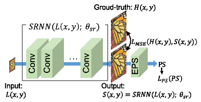
Figure 2: Deep SR network with the MSE loss ($L_{MSE}$) and our explicit perceptual loss ($L_{PS}$). “EPS” in the figure outputs the explicit perceptual score of each reconstructed SR image, $S(x,y)$. $\theta_{sr}$ denotes the parameters of the network.

In this section, we propose how to use the two explicit perceptual metrics, NIQE and MSD, as loss functions that are applicable to deep SR networks. A simple illustration of the SR network is shown in Figure 2. Basic SR networks such as SRCNN and DBPN employ only the MSE loss, which is $L_{MSE}=\frac{1}{XY}\sum^{X,Y}_{x,y}\left(S(x,y)-H(x,y)\right)^{2}$ in this figure where $S(x,y)$ and $H(x,y)$ denote the SR and ground-truth high-resolution (HR) images, each of whose size is $(X,Y)$, respectively.

Since NIQE outputs a scalar score (i.e., $D(\nu_{n},\nu_{t},\Sigma_{n},\Sigma_{t})$ in (4)) only based on statistic calculation, $D(\nu_{n},\nu_{t},\Sigma_{n},\Sigma_{t})$ can be directly used as a loss function for deep SR networks. In this case, “EPS” in Figure 2 consists of Equations (1), (2), (3), and (4).

In MSD, on the other hand, a ML based regressor is employed at the final stage. Any type of regressors can be employed, including deep networks, random forests, support vector machines, and so on. For example, the Ma’s algorithm uses random forest regressors for all metrics. Depending on the type of the regressor, we propose the following two options for using MSD as a loss function:

Deep networks:

As with NIQE, the MSD regressor using a deep network that outputs a scalar MSD score can be straightforwardly combined with deep SR networks. In this case, “EPS” in Figure 2 indicates the MSD regressor using the deep network.

Other ML algorithms:

We have difficulty in containing other ML algorithms into a deep network both for efficient training and inference. Our proposed method resolves this problem by employing a MSD feature vector instead of a MSD score. The MSD feature vector is computed from any image. In the training stage, we compute the MSE loss between the MSD feature vectors of each reconstructed image and its original HR image in “EPS” in Figure 2. This loss is used for evaluating the perceptual quality of each reconstructed SR image While the MSD feature vector is computed from every reconstructed SR image, the one of the HR image is computed only once at the beginning of the training stage.

Finally, the loss function with NIQE and MSD is defined as follows:

$$L_{PS}=\epsilon\left(D(\nu_{n},\nu_{t},\Sigma_{n},\Sigma_{t})\right)^{2}+\zeta L_{Ma},$$ (5)

where $\epsilon$ and $\zeta$ denote the weights of NIQE and MSD, respectively, and $L_{Ma}$ is either of the following ones:

Deep networks:

$$L_{Ma}=PSNN(M^{S}),$$ (6)

where $PSNN(M^{S})$ denotes the deep network that regresses the perceptual score from $M^{S}$, which is the MSD feature vector of the reconstructed SR. $PSNN(M^{S})$ is trained so that a lower score means the better perceptual quality.

Other ML algorithms:

$$L_{Ma}=\sum_{i}\left(M^{S}_{i}-M^{H}_{i}\right)^{2},$$ (7)

where $M^{H}$ denotes the MSD feature vector of the original HR image.

These two options, Eqs (6) and (7), are evaluated in Section 4.3.

4 Experimental Results

4.1 Implementation and training details

The networks consist of two blocks: generator ($G$) and discriminator ($D$) [9]. $G$ network generates (SR) images and $D$ network differentiates between real (HR) and fake (SR) images. DBPN [11], the winner of SR competition held in 2018 [33, 3], was used as $G$ network. Meanwhile, $D$ network consists of five hidden layers with batch norm and the last layer is fully connected layer. The training mechanism is illustrated in Fig. 3.

We trained the networks using images from DIV2K [1] with online augmentation (scaling, rotating, flipping, and random cropping). To produce LR images, we downscale the HR images on particular scaling factors using Bicubic. We use the validation set from PIRM2018 [3] as the test set which consists of 100 images.

The experiment focuses on 4$\times$ scaling factor. We use DBPN-S which is the variant of DBPN with shallower depth. On DBPN-S, we use $8\times 8$ kernel with stride = 4 and pad by 2 pixels with T = 2. All convolutional and transposed convolutional layers are followed by parametric rectified linear units (PReLUs), except the final reconstruction layer. We initialize the weights based on [15].

We use batch size of 4 with size $576\times 576$ for HR image, while LR image size is 144 $\times$ 144. We intentionally use big size patches assuming explicit perceptual loss works better on bigger patch than on the smaller patches as shown in Fig. 3. The learning rate is initialized to $1e-4$ for all layers and decrease by a factor of 10 for every 50 epochs for total 100 epochs. We used Adam with momentum to $0.9$. All experiments were conducted using PyTorch 0.4.1 and Python 3.5 on NVIDIA TITAN X GPUs.

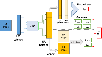
Figure 3: The overview of training mechanism.

To evaluate the performance, we use Perceptual score proposed in PIRM2018 [3], the perceptual super-resolution challenge. It is divided into three categories defined by thresholds on the RMSE. The three region are defined by Region 1: RMSE $\leq 11.5$ , Region 2: $11.5<$ RMSE $\leq 12.5$, and Region 3: $12.5<$ RMSE $\leq 16$. The Perceptual score is computed by combining the quality measures of Ma [24] and NIQE [26] as below. A lower score means the better perceptual quality.

$$\texttt{Perceptual score}=1/2((10-Ma)+NIQE)$$ (8)

4.2 Combination on multiple loss functions

Here, we evaluate the combination of five losses function on G network to show the characteristic of each loss, producing 32 combinations. On G network, we implement six losses (MSE, VGG, Style, Adversarial loss, NIQE, and Ma) which explained as below.

$$\begin{split}L_{G}&=10*L_{mse}+w_{1}*L_{vgg}+w_{2}*L_{adv}+\\ &w_{3}*L_{style}+w_{4}*L_{NIQE}+w_{5}*L_{Ma}\end{split}$$ (9)

(a) $L_{mse}$

is pixel-wise loss $L_{mse}=||I^{h}-I^{sr}||^{2}_{2}$.

(b) $L_{vgg}$

is calculated in the feature space using pretrained VGG19 [31] on multiple layers. This loss was originally proposed by [19, 6]. Both $I^{h}$ and $I^{sr}$ are first mapped into a feature space by differentiable functions $f_{i}$ from VGG multiple max-pool layers ${(i={2,3,4,5})}$ then sum up each layer distances. $L_{vgg}=\sum\limits_{i={2}}^{5}||f_{i}(I^{h})-f_{i}(I^{sr})||^{2}_{2}$.

(c) $L_{adv}$

$=-\texttt{log}(D(G(I^{l})))$ [9]

(d) $L_{style}$

is used to generate high quality textures [8].

(e) $L_{NIQE}$

(Eqs. 4)

(f) $L_{Ma}$

(Eqs. 5)

For $D$ network [9], it is optimized by

$$\begin{split}L_{D}=-\texttt{log}(D(I^{h}))-\texttt{log}(1-D(G(I^{l})))\end{split}$$ (10)

Table 1 shows the results on 32 combinations. It is hard to interpret the behavior of loss function. However, some results can be highlighted to generally understand the characteristic of each loss, especially between implicit and explicit perceptual loss. Noted that the weight for each loss is chosen based on preliminary experiments.

Among a single loss function (no. 1 - 6), it is shown that $L_{NIQE}$ provides the best results on Region 2. Further improvement can be achieved when we combined explicit perceptual loss with $L_{adv}$ as shown in no. 12. However, we start observing diminishing returns on $L_{NIQE}$ even combined with other implicit perceptual loss. Meanwhile, $L_{Ma}$ shows good performance only if combined with $L_{vgg}$ and $L_{adv}$.

The best combination is shown on no. 19 which use four loss functions: $L_{mse}$, $L_{vgg}$,$L_{adv}$, and $L_{Ma}$. It is also interesting to see that the second best result is no. 17 which also use four loss functions but replacing $L_{Ma}$ with $L_{style}$. Therefore, we can conclude that $L_{Ma}$ is able to replace $L_{style}$ with a marginal improvement.

The best result on two explicit perceptual loss is shown by no. 31. However, it is important to note that $L_{adv}$ is crucial to improve the performance of this combination. We can clearly see it by comparing no. 31 and 30 where no. 30’s performance is much worse by only eliminating $L_{adv}$.

Table 1: The comparison of six losses on 32 combinations.

No.	$w_{1}$	$w_{2}$	$w_{3}$	$w_{4}$	$w_{5}$	Perc.	RMSE	Region
1	0	0	0	0	0	5.692	11.86	2
2	0.1	0	0	0	0	5.654	11.82	2
3	0	0.1	0	0	0	2.540	14.12	3
4	0	0	10	0	0	5.699	11.76	2
5	0	0	0	0.01	0	5.397	11.86	2
6	0	0	0	0	0.001	5.666	11.89	2
7	0.1	0.1	0	0	0	2.751	13.86	3
8	0.1	0	10	0	0	5.784	12.1	2
9	0.1	0	0	0.01	0	5.587	12.13	2
10	0.1	0	0	0	0.001	5.713	11.81	2
11	0	0.1	10	0	0	2.580	13.9	3
12	0	0.1	0	0.01	0	2.575	13.73	3
13	0	0.1	0	0	0.001	5.745	11.79	2
14	0	0	10	0.01	0	5.557	11.98	2
15	0	0	10	0	0.001	5.685	11.89	2
16	0	0	0	0.01	0.001	5.506	11.94	2
17	0.1	0.1	10	0	0	2.479	13.86	3
18	0.1	0.1	0	0.01	0	2.562	14.44	3
19	0.1	0.1	0	0	0.001	2.471	14.07	3
20	0.1	0	10	0.01	0	5.733	11.82	2
21	0.1	0	10	0	0.001	5.657	11.77	2
22	0.1	0	0	0.01	0.001	5.533	11.85	2
23	0	0.1	10	0.01	0	2.580	13.98	3
24	0	0	10	0.01	0.001	5.459	11.85	2
25	0	0.1	0	0.01	0.001	2.626	14.27	3
26	0	0.1	10	0	0.001	3.089	13.80	3
27	0.1	0.1	10	0.01	0	2.724	13.78	3
28	0.1	0.1	10	0	0.001	2.549	13.78	3
29	0.1	0.1	0	0.01	0.001	2.507	13.84	3
30	0.1	0	10	0.01	0.001	5.614	11.86	2
31	0	0.1	10	0.01	0.001	2.497	13.81	3
32	0.1	0.1	10	0.01	0.001	2.537	14.03	3

4.3 Different type of regressor on explicit perceptual loss

We conduct experiment to evaluate two types of regressor on explicit perceptual loss. Here, the network is only optimized by one loss, either NN (6) or other ML (7). The results are shown in Table 2. (6) approach has a marginal decline compare with (7). It can be assumed that (7) performed better than (6). Furthermore, (7) provide low computation and less hyperparameter are needed to ease the optimization process.

Table 2: The comparison of different type of the regressor for explicit perceptual loss.

Method	Perceptual Score	RMSE
NN (6)	5.729	11.83
other ML (7)	5.666	11.90

4.4 Subjective evaluation

We performed a subjective test to quantify the performance of different combination of loss function. Specifically, we asked 30 raters to assign a score from 1 (bad quality) to 10 (best quality) to each image. The raters rated 7 combinations of loss function: $L_{mse}$, $L_{mse}+L_{vgg}$, $L_{mse}+L_{adv}$, $L_{mse}+L_{style}$, $L_{mse}+L_{NIQE}$, $L_{mse}+L_{Ma}$, $L_{mse}+L_{vgg}+L_{adv}+L_{style}+L_{NIQE}+L_{Ma}$. In total, each raters rated 700 instances (7 combinations of 100 images).

The result of subjective evaluation is shown in Fig. 5. Most of the raters give a lower score for “MSE+Adv” and “All”, while there are slight differences between other methods. The best subjective score is achieved by “MSE+Style”. On Section 4.2, it shows that explicit perceptual loss is able to improve the perceptual score. However, the subjective evaluation shows that better perceptual score does not give better visualization on human perception.

This result produces at least two observations. From this evaluation, it shows there is no strong correlation between the existing perceptual score and subjective evaluation. Other observation shows the explicit perceptual loss tends to generate high frequency artifacts which is considered as a noise on human perception as shown in Fig. 4.

(a) GT	(b) LR
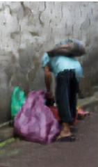
(c) MSE	(d) Implicit

Figure 4: The comparison of different loss function. The implicit perceptual loss tends to create high-frequency artifacts which can be considered as noise by human perception.

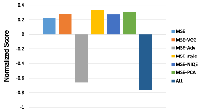
Figure 5: The result of subjective test.

5 Concluding Remarks

We proposed an explicit way to utilize machine learning model which trained to produce the perceptual score on generated SR images.s The experimental results show the proposed approach is able to improve the perceptual score better than the implicit approaches. We further show the characteristic of implicit and explicit perceptual loss for easier interpretation. We also demonstrate that the existing perceptual score does not correlate well with human perception using subjective evaluation. The results open more challenges to create better image quality metrics which can be used explicitly to optimize the SR network.

Future work includes an extension of this work to other SR problems (i.e., video SR [27, 13, 17], time SR [18, 38], and space-time SR [14, 35]).

This work is partly supported by JSPS KAKENHI Grant Number 19K12129.

References

- [1] E. Agustsson and R. Timofte. Ntire 2017 challenge on single image super-resolution: Dataset and study. In The IEEE Conference on Computer Vision and Pattern Recognition (CVPR) Workshops, July 2017.
- [2] Y. Blau, R. Mechrez, R. Timofte, T. Michaeli, and L. Zelnik-Manor. 2018 PIRM challenge on perceptual image super-resolution. arXiv, abs/1809.07517, 2018.
- [3] Y. Blau, R. Mechrez, R. Timofte, T. Michaeli, and L. Zelnik-Manor. 2018 pirm challenge on perceptual image super-resolution. arXiv preprint arXiv:1809.07517, 2018.
- [4] Y. Blau and T. Michaeli. The perception-distortion tradeoff. In CVPR, 2018.
- [5] X. Deng, R. Yang, M. Xu, and P. L. Dragotti. Wavelet domain style transfer for an effective perception-distortion tradeoff in single image super-resolution. In ICCV, pages 3076–3085. IEEE, 2019.
- [6] A. Dosovitskiy and T. Brox. Generating images with perceptual similarity metrics based on deep networks. In Advances in Neural Information Processing Systems, pages 658–666, 2016.
- [7] Y. Fang, J. Liu, Y. Zhang, W. Lin, and Z. Guo. Quality assessment for image super-resolution based on energy change and texture variation. In ICIP, 2016.
- [8] L. A. Gatys, A. S. Ecker, and M. Bethge. Image style transfer using convolutional neural networks. In Proceedings of the IEEE Conference on Computer Vision and Pattern Recognition, pages 2414–2423, 2016.
- [9] I. Goodfellow, J. Pouget-Abadie, M. Mirza, B. Xu, D. Warde-Farley, S. Ozair, A. Courville, and Y. Bengio. Generative adversarial nets. In Advances in neural information processing systems, pages 2672–2680, 2014.
- [10] S. Gu et al. AIM 2019 challenge on image extreme super-resolution: Methods and results. In ICCV Workshop, pages 3556–3564. IEEE, 2019.
- [11] M. Haris, G. Shakhnarovich, and N. Ukita. Deep back-projection networks for super-resolution. In CVPR, 2018.
- [12] M. Haris, G. Shakhnarovich, and N. Ukita. Deep back-projection networks for single image super-resolution. arXiv, abs/1904.05677, 2019.
- [13] M. Haris, G. Shakhnarovich, and N. Ukita. Recurrent back-projection network for video super-resolution. In CVPR, pages 3897–3906. Computer Vision Foundation / IEEE, 2019.
- [14] M. Haris, G. Shakhnarovich, and N. Ukita. Space-time-aware multi-resolution video enhancement. In CVPR, pages 2856–2865. IEEE, 2020.
- [15] K. He, X. Zhang, S. Ren, and J. Sun. Delving deep into rectifiers: Surpassing human-level performance on imagenet classification. In Proceedings of the IEEE International Conference on Computer Vision, pages 1026–1034, 2015.
- [16] M. Irani and S. Peleg. Improving resolution by image registration. CVGIP: Graph. Models Image Process., 53(3):231–239, Apr. 1991.
- [17] T. Isobe, X. Jia, S. Gu, S. Li, S. Wang, and Q. Tian. Video super-resolution with recurrent structure-detail network. In ECCV, 2020.
- [18] H. Jiang, D. Sun, V. Jampani, M. Yang, E. G. Learned-Miller, and J. Kautz. Super slomo: High quality estimation of multiple intermediate frames for video interpolation. In CVPR, pages 9000–9008. IEEE Computer Society, 2018.
- [19] J. Johnson, A. Alahi, and L. Fei-Fei. Perceptual losses for real-time style transfer and super-resolution. In European Conference on Computer Vision, pages 694–711. Springer, 2016.
- [20] L. Kang, P. Ye, Y. Li, and D. S. Doermann. Convolutional neural networks for no-reference image quality assessment. In CVPR, 2014.
- [21] C. Ledig, L. Theis, F. Huszar, J. Caballero, A. Cunningham, A. Acosta, A. P. Aitken, A. Tejani, J. Totz, Z. Wang, and W. Shi. Photo-realistic single image super-resolution using a generative adversarial network. In CVPR, 2017.
- [22] A. Lugmayr, M. Danelljan, L. V. Gool, and R. Timofte. Srflow: Learning the super-resolution space with normalizing flow. In ECCV, 2020.
- [23] H. Luo. A training-based no-reference image quality assessment algorithm. In ICIP, 2004.
- [24] C. Ma, C. Yang, X. Yang, and M. Yang. Learning a no-reference quality metric for single-image super-resolution. Computer Vision and Image Understanding, 158:1–16, 2017.
- [25] K. Ma, W. Liu, K. Zhang, Z. Duanmu, Z. Wang, and W. Zuo. End-to-end blind image quality assessment using deep neural networks. IEEE Trans. Image Processing, 27(3):1202–1213, 2018.
- [26] A. Mittal, R. Soundararajan, and A. C. Bovik. Making a ”completely blind” image quality analyzer. IEEE Signal Process. Lett., 20(3):209–212, 2013.
- [27] S. Nah et al. NTIRE 2019 challenge on video super-resolution: Methods and results. In CVPR Workshop, pages 1985–1995. Computer Vision Foundation / IEEE, 2019.
- [28] A. R. Reibman, R. M. Bell, and S. Gray. Quality assessment for super-resolution image enhancement. In ICIP, 2006.
- [29] D. L. Ruderman. The statistics of natural images. Network Computation in Neural Syst., 5:517–548, 1994.
- [30] M. S. M. Sajjadi, B. Schölkopf, and M. Hirsch. Enhancenet: Single image super-resolution through automated texture synthesis. In ICCV, 2017.
- [31] K. Simonyan and A. Zisserman. Very deep convolutional networks for large-scale image recognition. ICLR, 2015.
- [32] H. Tang, N. Joshi, and A. Kapoor. Blind image quality assessment using semi-supervised rectifier networks. In CVPR, 2014.
- [33] R. Timofte, S. Gu, J. Wu, and L. V. Gool. NTIRE 2018 challenge on single image super-resolution: Methods and results. In CVPR Workshop, 2018.
- [34] Z. Wang, A. C. Bovik, H. R. Sheikh, and E. P. Simoncelli. Image quality assessment: from error visibility to structural similarity. IEEE Trans. Image Processing, 13(4):600–612, 2004.
- [35] X. Xiang, Y. Tian, Y. Zhang, Y. Fu, J. P. Allebach, and C. Xu. Zooming slow-mo: Fast and accurate one-stage space-time video super-resolution. In CVPR, pages 3367–3376. IEEE, 2020.
- [36] H. Yeganeh, M. Rostami, and Z. Wang. Objective quality assessment for image super-resolution: A natural scene statistics approach. In ICIP, 2012.
- [37] K. Zhang et al. NTIRE 2020 challenge on perceptual extreme super-resolution: Methods and results. In CVPR Workshop, pages 2045–2057. IEEE, 2020.
- [38] L. P. Zuckerman, E. Naor, G. Pisha, S. Bagon, and M. Irani. Across scales & across dimensions: Temporal super-resolution using deep internal learning. In ECCV, 2020.