Determination of $\alpha_{S}$ beyond NNLO using event shape averages

Abstract

We consider a method for determining the QCD strong coupling constant using fits of perturbative predictions for event shape averages to data collected at the LEP, PETRA, PEP and TRISTAN colliders. To obtain highest accuracy predictions we use a combination of perturbative ${\cal{O}}(\alpha_{S}^{3})$ calculations and estimations of the ${\cal{O}}(\alpha_{S}^{4})$ perturbative coefficients from data. We account for non-perturbative effects using modern Monte Carlo event generators and analytic hadronization models. The obtained results show that the total precision of the $\alpha_{S}$ determination cannot be improved significantly with the higher order perturbative QCD corrections alone, but primarily requires a deeper understanding of the non-perturbative effects.

MPP-2020-167

1 Introduction

Measurements using hadronic final states in $e^{+}e^{-}$ annihilation have provided detailed experimental tests of Quantum Chromodynamics (QCD), the theory of the strong interaction in the Standard Model. These measurements were based on comparisons of moments and differential distributions of event shapes or jet rates to perturbative predictions. As new data are not foreseen in the near future, the progress in such measurements depends wholly on improvements in the theoretical (and phenomenological) description of these observables. Moreover, in multiple QCD analyses of the LEP data in the past, it was shown that the experimental uncertainties play a relatively small role in comparison to the theory-related uncertainties.

This situation rises some important questions. First of all, would the increasingly precise perturbative QCD (pQCD) calculations amended with resummation techniques be able to improve the precision of the results in QCD studies without any new data? And if not, what would be the limiting factors for the precision of QCD studies in the future and what should be done to eliminate them? To answer these questions we perform a QCD analysis with state-of-the-art pQCD calculations extended with estimations of higher-order corrections not known at present.

Fully differential pQCD calculations for the production of three partonic jets in $e^{+}e^{-}$ hadronic annihilation are available to ${\cal O}(\alpha_{S}^{3})$ accuracy [1, 2, 3, 4, 5, 6], which corresponds to next-to-next-to-leading order (NNLO) in QCD perturbation theory for this process. Four- and five-jet production [7, 8, 9, 10, 11, 12], as well as the total cross section [13] are also known including terms at ${\cal O}(\alpha_{S}^{3})$, therefore it is possible to make predictions for any infrared-safe observable at this level of accuracy. Although higher-order corrections are presently not known, it is in principle possible to estimate such corrections from data and therefore to obtain “predictions” at ${\cal O}(\alpha_{S}^{4})$. This approach is obviously limited to cases of observables for which only a small number of coefficients of the perturbative expansion should be estimated, such as event shape moments. In this paper we present an implementation of this approach with the aim of assessing the impact of these terms on possible future extractions of the strong coupling with exact predictions at ${\cal O}(\alpha_{S}^{4})$.

When confronting calculations based on QCD perturbation theory (of any order) with data, it must be kept in mind that although in $e^{+}e^{-}$ annihilation strong interactions occur only in the final state, nevertheless, the observed quantities are affected by hadronization and power corrections. These corrections must either be extracted from Monte Carlo predictions or computed using analytic models. Below, we consider both of these approaches for describing non-perturbative effects and perform simultaneous fits of $\alpha_{S}(M_{Z})$ and the ${\cal O}(\alpha_{S}^{4})$ perturbative coefficients to event shape moments (together with model parameters for analytic hadronization models) for thrust [16, 17] and the $C$-parameter [18, 19].

Anticipating some of our findings, we observe a clear discrepancy between results obtained with fits using Monte Carlo and analytic hadronization models, even after the inclusion of higher orders in pQCD and extending the analytic models to ${\cal O}(\alpha_{S}^{4})$. This implies that efforts to significantly improve the overall precision of $\alpha_{S}$ extractions in the future must address not only the computation of higher-order pQCD corrections, but also the refined modeling of non-perturbative effects.

We expect that the presented analysis will provide valuable input for the planing of $\alpha_{S}(M_{Z})$ measurements and data taking at future $e^{+}e^{-}$ facilities.

2 Theory predictions

The $n$-th moment of an event shape variable $O$ is defined by

$$\langle O^{n}\rangle=\frac{1}{\sigma_{\mathrm{tot}}}\int_{O_{\mathrm{min}}}^{O_{\mathrm{max}}}O^{n}\frac{\mathrm{d}\sigma(O)}{\mathrm{d}O}\mathrm{d}O,$$

where $\sigma_{\mathrm{tot}}$ stands for the total hadronic cross section and $[O_{\mathrm{min}},O_{\mathrm{max}}]$ is the kinematically allowed range of the observable $O$.

The fixed-order prediction for the $n$-th moment of $O$ at a reference renormalization scale $\mu=\mu_{0}$, normalized to the LO cross section $\sigma_{0}$ for $e^{+}e^{-}\to\mbox{hadrons}$ reads:

$$\begin{split}\frac{1}{\sigma_{0}}\int_{O_{\mathrm{min}}}^{O_{\mathrm{max}}}O^{n}\frac{\mathrm{d}\sigma(O)}{\mathrm{d}O}\mathrm{d}O&=\frac{\alpha_{S}(\mu_{0})}{2\pi}A^{{\langle O^{n}\rangle}}_{0}+\left(\frac{\alpha_{S}(\mu_{0})}{2\pi}\right)^{2}B^{{\langle O^{n}\rangle}}_{0}+\left(\frac{\alpha_{S}(\mu_{0})}{2\pi}\right)^{3}C^{{\langle O^{n}\rangle}}_{0}\\ &+\left(\frac{\alpha_{S}(\mu_{0})}{2\pi}\right)^{4}D^{{\langle O^{n}\rangle}}_{0}+{\cal O}(\alpha_{S}^{5}).\end{split}$$

Throughout the paper we employ the $\overline{\mathrm{MS}}$ renormalization scheme and $\alpha_{S}$ (without a superscript) always denotes the strong coupling in this scheme. The coefficients $A^{\langle O^{n}\rangle}_{0}$, $B^{\langle O^{n}\rangle}_{0}$ and $C^{\langle O^{n}\rangle}_{0}$ for moments of standard event shapes have been known for some time [2, 4]. In this paper, we use the CoLoRFulNNLO [20, 21, 6] approach to recompute these coefficients with high numerical precision, see Tab. 1.

Coefficient	This work	Analytic	Ref. [2]	Ref. [4]
$A^{{\langle(1-T)^{1}\rangle}}_{0}$	2.1034(1)	2.1034701	2.1035	2.10344(3)
$B^{{\langle(1-T)^{1}\rangle}}_{0}$	44.995(1)		44.999(2)	44.99(5)
$C^{{\langle(1-T)^{1}\rangle}}_{0}$	979.6(6)		867(21)	1100(30)
$A^{{\langle C^{1}\rangle}}_{0}$	8.6332(5)	8.6378902	8.6379	8.6378(1)
$B^{{\langle C^{1}\rangle}}_{0}$	172.834(5)	172.85900	172.778(7)	172.8(3)
$C^{{\langle C^{1}\rangle}}_{0}$	3525(3)		3212(88)	4200(100)
$A^{{\langle(1-T)^{2}\rangle}}_{0}$	0.19019(1)	0.1901961	0.1902	0.190190(5)
$B^{{\langle(1-T)^{2}\rangle}}_{0}$	6.25943(7)		6.2595(4)	6.2568(4)
$C^{{\langle(1-T)^{2}\rangle}}_{0}$	175.17(5)		172(1)	182.9(2)
$A^{{\langle C^{2}\rangle}}_{0}$	2.4316(1)	2.4316479	2.4317	2.43160(4)
$B^{{\langle C^{2}\rangle}}_{0}$	81.1882(9)		81.184(5)	81.160(5)
$C^{{\langle C^{2}\rangle}}_{0}$	2231.7(6)		2220(12)	2332(2)
$A^{{\langle(1-T)^{3}\rangle}}_{0}$	0.029875(2)	0.0298753	0.02988	0.029874(1)
$B^{{\langle(1-T)^{3}\rangle}}_{0}$	1.12852(1)		1.1284(1)	1.1278(1)
$C^{{\langle(1-T)^{3}\rangle}}_{0}$	34.71(1)		35.3(2)	36.17(3)
$A^{{\langle C^{3}\rangle}}_{0}$	1.07919(7)	1.0792137	1.0792	1.07919(3)
$B^{{\langle C^{3}\rangle}}_{0}$	42.7709(4)		42.771(3)	42.752(3)
$C^{{\langle C^{3}\rangle}}_{0}$	1304.4(3)		1296(6)	1360.8(8)
$A^{{\langle(1-T)^{4}\rangle}}_{0}$	0.0058583(6)	0.0058581	0.005858	0.0058576(3)
$B^{{\langle(1-T)^{4}\rangle}}_{0}$	0.246380(4)		0.24637(3)	0.24619(5)
$C^{{\langle(1-T)^{4}\rangle}}_{0}$	8.142(3)		8.13(4)	8.447(8)
$A^{{\langle C^{4}\rangle}}_{0}$	0.56849(4)	0.5685012	0.5685	0.56848(2)
$B^{{\langle C^{4}\rangle}}_{0}$	25.8174(3)		25.816(2)	25.804(3)
$C^{{\langle C^{4}\rangle}}_{0}$	845.4(1)		843(3)	879.1(5)
$A^{{\langle(1-T)^{5}\rangle}}_{0}$	0.0012948(1)	0.0012947	0.001295	0.0012946(9)
$B^{{\langle(1-T)^{5}\rangle}}_{0}$	0.060085(1)		0.06009(1)	0.06003(2)
$C^{{\langle(1-T)^{5}\rangle}}_{0}$	2.1170(9)		2.109(9)	2.184(2)
$A^{{\langle C^{5}\rangle}}_{0}$	0.32721(3)	0.3272163	0.3272	0.32720(1)
$B^{{\langle C^{5}\rangle}}_{0}$	16.8743(2)		16.873(1)	16.865(3)
$C^{{\langle C^{5}\rangle}}_{0}$	586.9(1)		585(3)	607.4(4)

Table 1: LO, NLO and NNLO contributions to the moments of event shapes. For the details on the analytic calculation see App. B.

This allows us to extend the extraction of the strong coupling constant from these observables to N³LO with a simultaneous extraction of the perturbative coefficients $D^{\langle O^{n}\rangle}_{0}$ from the data.

However, the experimentally measured event shape moments are normalized to the total hadronic cross section, and the perturbative expansion of $\langle O^{n}\rangle$ is given by

$$\begin{split}\langle O^{n}\rangle&=\frac{\alpha_{S}(\mu_{0})}{2\pi}\bar{A}^{\langle O^{n}\rangle}_{0}+\left(\frac{\alpha_{S}(\mu_{0})}{2\pi}\right)^{2}\bar{B}^{\langle O^{n}\rangle}_{0}+\left(\frac{\alpha_{S}(\mu_{0})}{2\pi}\right)^{3}\bar{C}^{\langle O^{n}\rangle}_{0}+\left(\frac{\alpha_{S}(\mu_{0})}{2\pi}\right)^{4}\bar{D}^{\langle O^{n}\rangle}_{0}\\ &+{\cal O}(\alpha_{S}^{5}).\end{split}$$

The relations between $\bar{A}^{\langle O^{n}\rangle}_{0}$, $\bar{B}^{\langle O^{n}\rangle}_{0}$, $\bar{C}^{\langle O^{n}\rangle}_{0}$, $\bar{D}^{\langle O^{n}\rangle}_{0}$ and $A^{\langle O^{n}\rangle}_{0}$, $B^{\langle O^{n}\rangle}_{0}$, $C^{\langle O^{n}\rangle}_{0}$, $D^{\langle O^{n}\rangle}_{0}$ are straightforward to obtain using

$$\begin{split}\frac{\sigma_{0}}{\sigma_{\mathrm{tot}}}&=1-\frac{\alpha_{S}}{2\pi}A_{\mathrm{tot}}+\left(\frac{\alpha_{S}}{2\pi}\right)^{2}\left(A_{\mathrm{tot}}^{2}-B_{\mathrm{tot}}\right)-\left(\frac{\alpha_{S}}{2\pi}\right)^{3}\left(A_{\mathrm{tot}}^{3}-2A_{\mathrm{tot}}B_{\mathrm{tot}}+C_{\mathrm{tot}}\right)+\mathcal{O}(\alpha_{S}^{4})\,,\end{split}$$

and we find

$$\bar{A}^{\langle O^{n}\rangle}_{0} =A^{\langle O^{n}\rangle}_{0}\,,$$

$$\bar{B}^{\langle O^{n}\rangle}_{0} =B^{\langle O^{n}\rangle}_{0}-A_{\mathrm{tot}}A^{\langle O^{n}\rangle}_{0}\,,$$

$$\bar{C}^{\langle O^{n}\rangle}_{0} =C^{\langle O^{n}\rangle}_{0}-A_{\mathrm{tot}}B^{\langle O^{n}\rangle}_{0}+\left(A_{\mathrm{tot}}^{2}-B_{\mathrm{tot}}\right)A^{\langle O^{n}\rangle}_{0}\,,$$

$$\bar{D}^{\langle O^{n}\rangle}_{0} =D^{\langle O^{n}\rangle}_{0}-A_{\mathrm{tot}}C^{\langle O^{n}\rangle}_{0}+\left(A_{\mathrm{tot}}^{2}-B_{\mathrm{tot}}\right)B^{\langle O^{n}\rangle}_{0}-\left(A_{\mathrm{tot}}^{3}-2A_{\mathrm{tot}}B_{\mathrm{tot}}+C_{\mathrm{tot}}\right)A^{\langle O^{n}\rangle}_{0}.$$

The coefficients $A_{\mathrm{tot}}$, $B_{\mathrm{tot}}$ and $C_{\mathrm{tot}}$ are listed in App. A.

Finally, to perform a simultaneous fit of multiple data points at different center-of-mass energies, we use the four-loop running of $\alpha_{S}(\mu)$

$$\mu^{2}\frac{d}{d\mu^{2}}\frac{\alpha_{S}(\mu)}{4\pi}=-\left(\frac{\alpha_{S}(\mu)}{4\pi}\right)^{2}\sum_{n}\beta_{n}\left(\frac{\alpha_{S}(\mu)}{4\pi}\right)^{n}\,,$$ (1)

with $\beta_{0}=(11C_{A}-2N_{F})/3$, $\beta_{1}=(34C_{A}^{2}-10C_{A}N_{F}-6C_{F}N_{F})/3$ and $\beta_{2}=(2857C_{A}^{3}-1415C_{A}^{2}N_{F}-615C_{A}C_{F}N_{F}+54C_{F}^{2}N_{F}+79C_{A}N_{F}^{2}+66C_{F}N_{F}^{2})/54$. We are using the customary normalization of $T_{R}=1/2$ for the color charge operators, thus in QCD we have $C_{A}=N_{c}=3$ and $C_{F}=(N_{c}^{2}-1)/(2N_{c})=4/3$, while $N_{F}$ denotes the number of light quark flavors. The corresponding dependence of the perturbative coefficients $\bar{A}^{\langle O^{n}\rangle}$, $\bar{B}^{\langle O^{n}\rangle}$, $\bar{C}^{\langle O^{n}\rangle}$ and $\bar{D}^{(n)}$ on scale read:

$$\bar{A}^{\langle O^{n}\rangle} =\bar{A}^{\langle O^{n}\rangle}_{0}\,,$$

$$\bar{B}^{\langle O^{n}\rangle} =\bar{B}_{0}^{\langle O^{n}\rangle}+\frac{1}{2}\bar{A}^{\langle O^{n}\rangle}_{0}\beta_{0}L\,,$$

$$\bar{C}^{\langle O^{n}\rangle} =\bar{C}_{0}^{\langle O^{n}\rangle}+\bar{B}^{\langle O^{n}\rangle}_{0}\beta_{0}L+\frac{1}{4}\bar{A}^{\langle O^{n}\rangle}_{0}(\beta_{1}+\beta_{0}^{2}L)L\,,$$

$$\bar{D}^{\langle O^{n}\rangle} =\bar{D}_{0}^{\langle O^{n}\rangle}+\frac{3}{2}\bar{C}_{0}^{\langle O^{n}\rangle}\beta_{0}L+\frac{1}{2}\bar{B}_{0}^{\langle O^{n}\rangle}\left(\beta_{1}+\frac{3}{2}\beta_{0}^{2}L\right)L$$ (2)

$$+\frac{1}{8}\bar{A}_{0}^{\langle O^{n}\rangle}\left(\beta_{2}+\frac{5}{2}\beta_{1}\beta_{0}L+\beta_{0}^{3}L^{2}\right)L,$$

where we have $L=\ln(\mu^{2}/\mu_{0}^{2})$.

We take into account the effect of non-vanishing $b$-quark mass on the predictions for the $A^{\langle O^{n}\rangle}$ and $B^{\langle O^{n}\rangle}$ coefficient by subtracting the fraction of $b$-quark events, $r_{b}(Q)$, from the massless result and adding back the corresponding massive prediction obtained with the Zbb4 [22] program,

$$A^{\langle O^{n}\rangle} =A^{\langle O^{n}\rangle}_{m_{b}=0}(1-r_{b}(Q))+r_{b}(Q)A^{\langle O^{n}\rangle}_{m_{b}\neq 0}\,,$$

$$B^{\langle O^{n}\rangle} =B^{\langle O^{n}\rangle}_{m_{b}=0}(1-r_{b}(Q))+r_{b}(Q)B^{\langle O^{n}\rangle}_{m_{b}\neq 0}\,.$$

3 Data sets

For the performed analysis, one minus thrust $\tau\equiv(1-T)$ and the $C$-parameter ($C$) were selected. The selection of these particular observables is motivated by the abundance of available measurements. More specifically, in this analysis we considered data sets from the ALEPH, AMY, DELPHI, HRS, JADE, L3, MARK, MARKII, OPAL and TASSO experiments, see Tab. 2 for details.

As the theory predictions for all the measured event shape moments were calculated in the CoLoRFulNNLO  framework and the hadronization corrections can be obtained consistently for all the event shape moments, the most complete analysis of the data might include simultaneously all the measured moments.

However, as most of the moments of the event shapes are quite strongly correlated [23], a simultaneous analysis of all available data would require taking these correlations into account. Unfortunately, very few data sets contain this crucial information and therefore, we have limited our analysis only to the first moments, i.e. averages of the event shapes. From the two available sets of measurements with the same data in the range $\sqrt{s}=133-183{\,\text{Ge}\kern-0.66666pt\text{V\/}}$, available from Ref. [24] and Ref. [25] the measurements from Ref. [25] were used in the analysis.

	Measured		Used
		Points,		Points,
Source	Observables	$\sqrt{s}$ range	Observables	$\sqrt{s}$ range
		(${\,\text{Ge}\kern-0.59999pt\text{V\/}})$		(${\,\text{Ge}\kern-0.59999pt\text{V\/}})$
ALEPH [26]	$\langle\tau^{1}\rangle$	$1$,$[133]$	$\langle\tau^{1}\rangle$	$1$,$[133]$
ALEPH [27]	$\langle\tau^{1}\rangle$	$1$,$[91]$	$\langle\tau^{1}\rangle$	$1$,$[91]$
ALEPH [28]	$\langle\tau^{1}\rangle$	$9$,$[91,206]$	$\langle\tau^{1}\rangle$	$9$,$[91,206]$
AMY [29]	$\langle\tau^{1}\rangle$	$1$,$[55]$	$\langle\tau^{1}\rangle$	$1$,$[55]$
DELPHI [25]	$\langle\tau^{1,2,3}\rangle$	$15$,$[91,183]$	$\langle\tau^{1}\rangle$	$5$,$[91,183]$
DELPHI [24]	$\langle\tau^{1}\rangle$	$15$,$[45,202]$	$\langle\tau^{1}\rangle$	$11$,$[45,202]$
HRS [30]	$\langle\tau^{1}\rangle$	$1$,$[29]$	$\langle\tau^{1}\rangle$	$1$,$[29]$
JADE [23]	$\langle\tau^{1,2,3,4,5}\rangle$	$30$,$[14,43]$	$\langle\tau^{1}\rangle$	$4$,$[34,43]$
L3 [31]	$\langle\tau^{1}\rangle$	$1$,$[91]$	$\langle\tau^{1}\rangle$	$1$,$[91]$
L3 [32]	$\langle\tau^{1,2}\rangle$	$30$,$[41,206]$	$\langle\tau^{1}\rangle$	$15$,$[41,206]$
MARK [33]	$\langle\tau^{1}\rangle$	$1$,$[89]$	$\langle\tau^{1}\rangle$	$1$,$[89]$
MARK [34]	$\langle\tau^{1}\rangle$	$1$,$[29]$	$\langle\tau^{1}\rangle$	$1$,$[29]$
MARKII [33]	$\langle\tau^{1}\rangle$	$1$,$[89]$	$\langle\tau^{1}\rangle$	$1$,$[89]$
OPAL [23]	$\langle\tau^{1,2,3,4,5}\rangle$	$60$,$[91,206]$	$\langle\tau^{1}\rangle$	$12$,$[91,206]$
TASSO [35]	$\langle\tau^{1}\rangle$	$4$,$[14,44]$	$\langle\tau^{1}\rangle$	$2$,$[35,44]$
ALEPH [27]	$\langle C^{1}\rangle$	$1$,$[91]$	$\langle C^{1}\rangle$	$1$,$[91]$
DELPHI [24]	$\langle C^{1}\rangle$	$15$,$[45,202]$	$\langle C^{1}\rangle$	$11$,$[45,202]$
DELPHI [25]	$\langle C^{1,2,3}\rangle$	$12$,$[133,183]$	$\langle C^{1}\rangle$	$4$,$[133,183]$
JADE [23]	$\langle C^{1,2,3,4,5}\rangle$	$30$,$[14,43]$	$\langle C^{1}\rangle$	$4$,$[34,43]$
L3 [31]	$\langle C^{1}\rangle$	$1$,$[91]$	$\langle C^{1}\rangle$	$1$,$[91]$
L3 [32]	$\langle C^{1,2}\rangle$	$18$,$[130,206]$	$\langle C^{1}\rangle$	$9$,$[130,206]$
OPAL [23]	$\langle C^{1,2,3,4,5}\rangle$	$60$,$[91,206]$	$\langle C^{1}\rangle$	$12$,$[91,206]$

Table 2: Available measurements and data used in the analysis. Here we use $\tau\equiv(1-T)$.

4 Modeling of non-perturbative corrections

As discussed in the Introduction, the modeling of non-perturbative corrections is essential in order to perform a meaningful comparison of theoretical predictions with data. One option for obtaining the hadronization corrections is to extract them from Monte Carlo simulations. Recent examples of this approach include the studies of the energy-energy correlation [36] and the two-jet rate [37].

Some previous extractions of the strong coupling from event shape moments [38, 23] and event shape distributions [39] have used an analytic hadronization model based on the dispersive approach to power corrections [40, 41, 42]. An important ingredient of this model is the relation between the strong coupling defined in the $\overline{\mathrm{MS}}$ scheme and the effective soft coupling $\alpha_{S}^{CMW}$ in the Catani–Marchesini–Webber (CMW) scheme. As the extension of $\alpha_{S}^{CMW}$ beyond NLL accuracy is believed not to be unique [43, 44], the coefficients in this relation are “scheme-dependent”. However, in one particular proposal, the relation between $\alpha_{S}$ and $\alpha_{S}^{CMW}$ has recently been computed up to $\mathcal{O}(\alpha_{S}^{4})$ accuracy [44], which allows us to implement a consistent analytic model of hadronization corrections at this order in the perturbative expansion.

Below, we pursue both options and use Monte Carlo tools as well as the analytic approach to estimate the non-perturbative corrections.

4.1 Monte Carlo hadronization models

In this work we use the Monte Carlo event generation setups similar to those in previous comparable studies [36]. We made use of the Herwig7.2.0 [45] and Sherpa2.2.8 [46] Monte Carlo event generators (MCEGs) with similar setups for perturbative calculations, but different hadronization models. The QCD matrix elements for the $e^{+}e^{-}\to Z/\gamma\to 2,3,4,5$ parton processes were generated using MadGraph5 [47] and the OpenLoops [48] one-loop library. The 2-parton final state process was computed at NLO accuracy in perturbative QCD. The generated events were hadronized using the Lund hadronization model [49] or the cluster hadronization model [50]. In the following, the setup labelled as $H^{L}$ denotes predictions computed with Herwig7.2.0 employing the Lund hadronization model [49], $H^{C}$ denotes Herwig7.2.0 predictions obtained with the cluster hadronization model [50], and finally $S^{C}$ denotes results obtained using Sherpa2.2.8 with the cluster hadronization model [51].

For the study, predictions of event shape moments were calculated from MC generated events at hadron and parton levels ($\langle O^{n}\rangle_{\mathrm{MC\ hadrons}}$ and ($\langle O^{n}\rangle_{\mathrm{MC\ partons}}$). To take into account that the presence of a shower cut-off $Q_{0}\approx{\cal O}(1{\,\text{Ge}\kern-0.66666pt\text{V\/}})$ in Monte Carlo programs affects the event shape distributions (e.g. see Refs. [52, 53]) both parton and hadron level MC predictions were calculated with several different values of the parton shower cut-offs and extrapolated to $Q_{0}\rightarrow 0{\,\text{Ge}\kern-0.66666pt\text{V\/}}$.

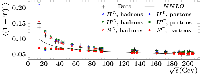
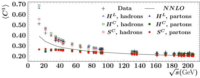
Figure 1: Data and predictions by MCEGs extrapolated to $Q_{0}=0{\,\text{Ge}\kern-0.66666pt\text{V\/}}$. The NNLO result was computed using $\alpha_{S}(M_{Z})=0.118$.

Fig. 1 shows the final results obtained with the various MCEG setups after extrapolation to $Q_{0}=0{\,\text{Ge}\kern-0.66666pt\text{V\/}}$, together with the experimental measurements. The hadron and parton level MC predictions seen in Fig. 1 provide reasonable descriptions of the data as well as the NNLO perturbative results for a wide range of center-of-mass energies. However, the MC predictions at lowest $\sqrt{s}$ show non-physical behavior, i.e. $\langle O^{n}\rangle$ increases with $\sqrt{s}$ for the parton level results. In order to analyze only the data that can be adequately described by the Monte Carlo modeling, we exclude measurements with $\sqrt{s}<29{\,\text{Ge}\kern-0.66666pt\text{V\/}}$ from the analysis. In practice this criterion is much weaker than a requirement that MC matches the data well or that the subleading power corrections to the analytic hadronization models are small. However, this choice, in addition to retaining as much of the data as is reasonable, serves to highlight the discrepancies between the Monte Carlo and analytic hadronization models in regions where hadronization effects are most pronounced, i.e. at low energies.

Finally, the correction of theory predictions for hadronization was implemented in the analysis as follows,

$$\langle O^{n}\rangle_{\mathrm{corrected}}=\langle O^{n}\rangle_{\mathrm{theory}}\times\frac{\langle O^{n}\rangle_{\mathrm{MC\ hadrons},\,Q_{0}=0{\,\text{Ge}\kern-0.46666pt\text{V\/}}}}{\langle O^{n}\rangle_{\mathrm{MC\ partons},\,Q_{0}=0{\,\text{Ge}\kern-0.46666pt\text{V\/}}}}\,.$$

The hadronization correction factors for different center-of-mass energies, observables and MC setups are shown in Fig. 2.

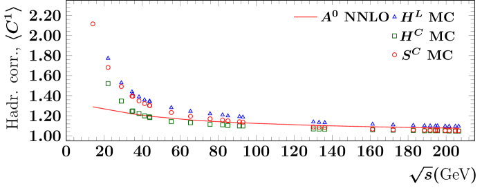
Figure 2: Hadronization corrections extracted from MC generated samples after extrapolation to $Q_{0}=0{\,\text{Ge}\kern-0.66666pt\text{V\/}}$ and the hadronization corrections from the ${\cal A}_{0}$ scheme calculated as ratios of the hadron and parton level predictions using $\alpha_{S}(M_{Z})=0.118$, $\alpha_{0}(\mu_{I})=0.5$ and $\mathcal{M}=1.49$. The hadronization corrections from the ${\cal A}_{T}$- and cusp-schemes are not shown, but these very closely follow the hadronization corrections from the ${\cal A}_{0}$-scheme.

4.2 Analytic hadronization models

The dispersive model of analytic hadronization corrections for event shapes in $e^{+}e^{-}$ annihilation has been worked out in detail in Refs. [40, 41, 42]. In this model, hadronization corrections simply shift the perturbative event shape distributions,

$$\frac{\mathrm{d}\sigma_{\mathrm{hadrons}}(O)}{\mathrm{d}O}=\frac{\mathrm{d}\sigma_{\mathrm{partons}}(O-a_{O}{\mathcal{P}})}{\mathrm{d}O},$$ (3)

where the power correction ${\mathcal{P}}$ is universal for all event shapes, while the $a_{O}$ are specific, known constants, e.g.  $a_{1-T}=2$ and $a_{C}=3\pi$ for $1-T$ and the $C$-parameter. Inserting eq. (3) into the definition of the moments, one obtains the non-perturbative predictions for event shape moments. In particular, the effect of hadronization corrections on the average is additive,

$$\langle O^{1}\rangle_{\mathrm{hadrons}}=\langle O^{1}\rangle_{\mathrm{partons}}+a_{O}\mathcal{P}\,,$$

where $\langle O^{1}\rangle_{\mathrm{partons}}$ is the value obtained in fixed-order perturbation theory as described in Sect. 2. Some deviations from this simple model were discussed very recently in Ref. [54].

Finally, we must compute the power correction ${\cal{P}}$ at $\mathcal{O}(\alpha_{S}^{4})$ accuracy. The perturbative ingredients of this calculation are the running of the strong coupling in the $\overline{\mathrm{MS}}$ scheme and the relation between the coupling defined in the $\overline{\mathrm{MS}}$ and the CMW schemes. This relation takes the following generic form

$$\alpha_{S}^{CMW}=\alpha_{S}\left[1+\frac{\alpha_{S}}{2\pi}K\right. +\left(\frac{\alpha_{S}}{2\pi}\right)^{2}L\left.+\left(\frac{\alpha_{S}}{2\pi}\right)^{3}M+\mathcal{O}(\alpha_{S}^{4})\right]\,.$$ (4)

The value of the $K$ coefficient has been known to coincide with the one-loop cusp anomalous dimension for a long time and hence it may be tempting to assume that the cusp anomalous dimension provides a sensible definition of the CMW coupling also beyond $\mathcal{O}(\alpha_{S}^{2})$. However, this assumption turns out to be incorrect and as mentioned above, it is believed that there is no unique extension of $\alpha_{S}^{CMW}$ beyond NLL accuracy. Nevertheless, recently several proposals have been made for the definition of the effective soft coupling in the literature [43, 44]. In particular, Ref. [44] introduces the effective soft-gluon coupling ${\mathcal{A}}_{i}^{CMW}$ as

$${\mathcal{A}}_{i}^{CMW}(\alpha_{S})=C_{i}\frac{\alpha_{S}^{CMW}}{\pi}=C_{i}\frac{\alpha_{S}}{\pi}\left(1+\frac{\alpha_{S}}{2\pi}K+\ldots\right)\,,$$

(here $i$ denotes the type of radiating parton, so $C_{q}=C_{F}$ and $C_{g}=C_{A}$) and proposes two different prescriptions for defining this coupling beyond NLL accuracy, denoted by $\mathcal{A}_{0,i}$ and $\mathcal{A}_{T,i}$. We will refer to these cases as the “$\mathcal{A}_{0}$-scheme” and the “$\mathcal{A}_{T}$-scheme” below. We note that the complete expression for the $M$ coefficient is currently not known in the $\mathcal{A}_{T}$-scheme, hence in our analysis we approximate this coefficient with its value in the $\mathcal{A}_{0}$-scheme and set $M_{T}=M_{0}$. In order to facilitate the comparison of our results with previous work [38], we also define the “cusp-scheme”, in which we simply set the $K$, $L$ and $M$ coefficients of eq. (4) equal to the appropriate cusp anomalous dimension. In the following, we will denote the results obtained in the $\mathcal{A}_{0}$-scheme by $A^{0}$, in the $\mathcal{A}_{T}$-scheme by $A^{T}$ and in the cusp-scheme by $A^{\mathrm{cusp}}$. The explicit expressions for the $K$, $L$ and $M$ coefficients in all three schemes are presented in App. C.

Finally, the power correction takes the following form up to N³LO,

$${\cal{P}}(\alpha_{S},Q,\alpha_{0}) =\frac{4C_{F}}{\pi^{2}}\,\mathcal{M}\times\frac{\mu_{I}}{Q}\times\,\bigg{\{}\alpha_{0}(\mu_{I})-\bigg{[}\alpha_{S}(\mu_{R})+\left(K+\beta_{0}\left(1+\ln\frac{\mu_{R}}{\mu_{I}}\right)\right)\frac{\alpha_{S}^{2}(\mu_{R})}{2\pi}$$

$$+\left(2L+\left(4\beta_{0}\left(\beta_{0}+K\right)+\beta_{1}\right)\left(1+\ln\frac{\mu_{R}}{\mu_{I}}\right)\right.\left.+2\beta_{0}^{2}\ln^{2}\frac{\mu_{R}}{\mu_{I}}\right)\frac{\alpha_{S}^{3}(\mu_{R})}{8\pi^{2}}$$

$$+\left(4M+\big{(}2\beta_{0}\left(12\beta_{0}(\beta_{0}+K)+5\beta_{1}\right)+\beta_{2}\right.\left.+4\beta_{1}K+12\beta_{0}L\big{)}\left(1+\ln\frac{\mu_{R}}{\mu_{I}}\right)\right.$$

$$+\beta_{0}(12\beta_{0}(\beta_{0}+K)+5\beta_{1})\ln^{2}\frac{\mu_{R}}{\mu_{I}}\left.+4\beta_{0}^{3}\ln^{3}\frac{\mu_{R}}{\mu_{I}}\right)\frac{\alpha_{S}^{4}(\mu_{R})}{32\pi^{3}}\bigg{]}\bigg{\}},$$ (5)

where $\mu_{I}$ is the scale at which the perturbative and non-perturbative couplings are matched in the dispersive model and $\mathcal{M}$ is the so-called Milan factor [42] with an estimated value of $\mathcal{M}_{\rm est.}\pm\delta\mathcal{M}_{\rm est.}=1.49\pm 0.30$ [42, 38]. $\alpha_{0}(\mu_{I})$ corresponds to the first moment of the effective coupling below the scale $\mu_{I}$

$$\alpha_{0}(\mu_{I})=\frac{1}{\mu_{I}}\int_{0}^{\mu_{I}}{\mathrm{d}}\mu\,\alpha^{CMW}(\mu)\,,$$

and it is a non-perturbative parameter of the model. Following the usual choice, we will set $\mu_{I}=2{\,\text{Ge}\kern-0.66666pt\text{V\/}}$. We note that the value of $\alpha_{0}(\mu_{I})$ is in principle scheme-dependent, i.e. it depends on the precise relation between the strong coupling in the $\overline{\mathrm{MS}}$ and CMW schemes. In contrast, $\alpha_{S}(\mu_{R})$ always refers to the value of the strong coupling in the $\overline{\mathrm{MS}}$ scheme, at scale $\mu_{R}$.

Before moving on, let us make two comments regarding eq. (5). First, it can be argued (see e.g. the discussion in ref. [39]) that the $L$ and $M$ coefficients that appear in ${\cal{P}}(\alpha_{S},Q,\alpha_{0})$ do not coincide precisely with those in eq. (4), but receive modifications due to the non-inclusive nature of the observables we are studying. As such, $L$ and $M$ in eq. (5) might be different for different observables. Second, beyond NLO, there is some doubt that the non-inclusive corrections parametrized by the Milan factor $\mathcal{M}$ can still be captured by a simple overall multiplicative factor in ${\cal{P}}(\alpha_{S},Q,\alpha_{0})$. Nevertheless, here we take the pragmatic viewpoint that eq. (5) provides a reasonable model for non-perturbative corrections. In particular, as in other analyses [38, 39], the Milan factor appears as a multiplicative constant. However, the applicability of this approach should be investigated in detail in future studies, either when new data or more precise estimations of the Milan factor become available.

5 Fit procedure and systematic uncertainties

The values of $\alpha_{S}$ were determined in the optimization procedures using the MINUIT2 [55, 56] program and the minimized function

$$\chi^{2}(\alpha_{S})=\sum^{\rm all\ data\ sets}_{i}\chi^{2}_{i}(\alpha_{S}),$$ (6)

where for data set $i$ we have $\chi^{2}_{i}(\alpha_{S})=(\vec{D}-\vec{P}(\alpha_{S}))V^{-1}(\vec{D}-\vec{P}(\alpha_{S}))^{T}$, with $\vec{D}$ standing for the vector of data points, $\vec{P}(\alpha_{S})$ for the vector of calculated predictions and $V$ for the covariance matrix of $\vec{D}$. In this analysis the covariance matrix $V$ was diagonal with the values of the diagonal elements calculated by adding the statistical and systematic uncertainties in quadrature for every measurement.

For all the fits with MC hadronization models the central results for $\alpha_{S}(M_{Z})$ (as well as the $D^{\langle O^{n}\rangle}$ coefficients in the N³LO fits) were extracted with the $H^{L}$ setup. The uncertainty on the fit result was estimated using the $\chi^{2}+1$ criterion as implemented in MINUIT2 ($exp.$). The systematic effects related to the modeling of hadronization with MCEGs were estimated as the difference of results obtained with $H^{L}$ and $H^{C}$ setups ($hadr.$). To estimate the systematic effects related to the choice of renormalization scale, the latter was varied by a factor of two in both directions ($scale$). The scale variation at N³LO was performed with the perturbative coefficients $D^{\langle O^{n}\rangle}$ fixed to their values obtained in the nominal fit. The uncertainty was estimated as half of the difference between the maximal and minimal obtained values among the three results.

When using the analytic hadronization model (with any of the three schemes discussed above), in addition to $\alpha_{S}(M_{Z})$ and $D^{\langle O^{n}\rangle}$, the quantities $\alpha_{0}(\mu_{I})$ and $\mathcal{M}$ were also treated as fit parameters to be extracted from data. Although the value of the Milan factor is in principle fixed by a theoretical calculation, including it as a constrained parameter in the fit provides a way of taking into account its uncertainty. For the fits with a constrained Milan factor a term $(\mathcal{M}-\mathcal{M}_{\rm est.})^{2}/(\delta\mathcal{M}_{\rm est.})^{2}$ is added to eq. (6).

As previously, the $\chi^{2}+1$ criterion was used to estimate the fit uncertainty ($exp.$), while the systematic effects of missing higher-order terms were estimated using the same renormalization scale variation procedure as for MC hadronization models ($scale.$). In particular, when varying the scale to estimate the related $\alpha_{S}(M_{Z})$ ($\alpha_{0}(\mu_{I})$) uncertainties, the $D^{\langle O^{n}\rangle}$ coefficients, $\alpha_{0}(\mu_{I})$ ($\alpha_{S}(M_{Z})$) and $\mathcal{M}$ were fixed to the values obtained in the nominal fits.

6 Results and discussion

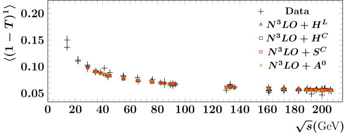
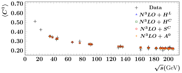
Figure 3: Data and fits obtained with different hadronization models. All available data points from Tab. 2 are shown.

The results of the NNLO and N³LO fits are presented in Tabs. 3 and 4, while the predictions of the N³LO fits for individual energy points are shown in Fig. 3.

Analysis	Results from analysis of $\langle(1-T)^{1}\rangle$ data
NNLO,	$\alpha_{S}(M_{Z})=0.11459\pm 0.00022{\text{(}exp.)}\pm 0.00024{\text{(}hadr.)}\pm 0.0025{\text{(}scale)}$
MC had.	$\chi^{2}/ndof=324.3/64$
$H^{L}$
NNLO,	$\alpha_{S}(M_{Z})=0.11927\pm 0.00125{\text{(}exp.)}\pm 0.0018{\text{(}scale)}$
analytic	$\chi^{2}/ndof=77.0/62$
had., $A^{0}$	$\alpha_{0}(2{\,\text{Ge}\kern-0.66666pt\text{V\/}})=0.48\pm 0.03{\text{(}exp.)}\pm 0.02{(scale)}$
	$\mathcal{M}=1.53\pm 0.30{\text{(}exp.)}$(constrained)
NNLO,	$\alpha_{S}(M_{Z})=0.11906\pm 0.00126{\text{(}exp.)}\pm 0.0017{\text{(}scale)}$
analytic	$\chi^{2}/ndof=76.9/62$
had., $A^{T}$	$\alpha_{0}(2{\,\text{Ge}\kern-0.66666pt\text{V\/}})=0.48\pm 0.03{\text{(}exp.)}\pm 0.02{(scale)}$
	$\mathcal{M}=1.53\pm 0.29{\text{(}exp.)}$(constrained)
NNLO,	$\alpha_{S}(M_{Z})=0.11940\pm 0.00125{\text{(}exp.)}\pm 0.0019{\text{(}scale)}$
analytic	$\chi^{2}/ndof=77.1/62$
had., $A^{\mathrm{cusp}}$	$\alpha_{0}(2{\,\text{Ge}\kern-0.66666pt\text{V\/}})=0.47\pm 0.03{\text{(}exp.)}\pm 0.025{(scale)}$
	$\mathcal{M}=1.53\pm 0.30{\text{(}exp.)}$(constrained)
N3LO,	$\alpha_{S}(M_{Z})=0.14092\pm 0.00116{\text{(}exp.)}\pm 0.00111{\text{(}hadr.)}\pm 0.0090{\text{(}scale)}$
MC had.	$\chi^{2}/ndof=79.2/63$
$H^{L}$	$D^{\langle(1-T)^{1}\rangle}=-7.51\times 10^{4}\pm 1.14\times 10^{3}{\text{(}exp.)}$
N3LO,	$\alpha_{S}(M_{Z})=0.12911\pm 0.00177{\text{(}exp.)}\pm 0.0123{\text{(}scale)}$
analytic	$\chi^{2}/ndof=76.3/61$
had., $A^{0}$	$D^{\langle(1-T)^{1}\rangle}=-9.36\times 10^{4}\pm 1.33\times 10^{4}{\text{(}exp.)}$
	$\alpha_{0}(2{\,\text{Ge}\kern-0.66666pt\text{V\/}})=0.89\pm 0.07{\text{(}exp.)}\pm 0.29{(scale)}$
	$\mathcal{M}=1.50\pm 0.17{\text{(}exp.)}$(constrained)
N3LO,	$\alpha_{S}(M_{Z})=0.12665\pm 0.00193{\text{(}exp.)}\pm 0.0096{\text{(}scale)}$
analytic	$\chi^{2}/ndof=76.3/61$
had., $A^{T}$	$D^{\langle(1-T)^{1}\rangle}=-7.97\times 10^{4}\pm 1.52\times 10^{4}{\text{(}exp.)}$
	$\alpha_{0}(2{\,\text{Ge}\kern-0.66666pt\text{V\/}})=0.84\pm 0.07{\text{(}exp.)}\pm 0.23{(scale)}$
	$\mathcal{M}=1.50\pm 0.19{\text{(}exp.)}$(constrained)
N3LO,	$\alpha_{S}(M_{Z})=0.13011\pm 0.00171{\text{(}exp.)}\pm 0.0137{\text{(}scale)}$
analytic	$\chi^{2}/ndof=76.3/61$
had., $A^{\mathrm{cusp}}$	$D^{\langle(1-T)^{1}\rangle}=-9.87\times 10^{4}\pm 1.26\times 10^{4}{\text{(}exp.)}$
	$\alpha_{0}(2{\,\text{Ge}\kern-0.66666pt\text{V\/}})=0.91\pm 0.07{\text{(}exp.)}\pm 0.31{(scale)}$
	$\mathcal{M}=1.50\pm 0.17{\text{(}exp.)}$(constrained)

Table 3: Results of the extraction analyses using the $\langle(1-T)^{1}\rangle$ observable.

Analysis	Results from analysis of $\langle C^{1}\rangle$ data
NNLO,	$\alpha_{S}(M_{Z})=0.11298\pm 0.00020{\text{(}exp.)}\pm 0.00019{\text{(}hadr.)}\pm 0.0022{\text{(}scale)}$
MC had.	$\chi^{2}/ndof=436.0/41$
$H^{L}$
NNLO,	$\alpha_{S}(M_{Z})=0.11958\pm 0.00120{\text{(}exp.)}\pm 0.0012{\text{(}scale)}$
analytic	$\chi^{2}/ndof=41.2/39$
had., $A^{0}$	$\alpha_{0}(2{\,\text{Ge}\kern-0.66666pt\text{V\/}})=0.43\pm 0.02{\text{(}exp.)}\pm 0.01{(scale)}$
	$\mathcal{M}=1.57\pm 0.29{\text{(}exp.)}$(constrained)
NNLO,	$\alpha_{S}(M_{Z})=0.11934\pm 0.00122{\text{(}exp.)}\pm 0.0011{\text{(}scale)}$
analytic	$\chi^{2}/ndof=41.0/39$
had. $A^{T}$	$\alpha_{0}(2{\,\text{Ge}\kern-0.66666pt\text{V\/}})=0.43\pm 0.02{\text{(}exp.)}\pm 0.01{(scale)}$
	$\mathcal{M}=1.57\pm 0.29{\text{(}exp.)}$(constrained)
NNLO,	$\alpha_{S}(M_{Z})=0.11973\pm 0.00119{\text{(}exp.)}\pm 0.0013{\text{(}scale)}$
analytic	$\chi^{2}/ndof=41.3/39$
had., $A^{\mathrm{cusp}}$	$\alpha_{0}(2{\,\text{Ge}\kern-0.66666pt\text{V\/}})=0.42\pm 0.02{\text{(}exp.)}\pm 0.01{(scale)}$
	$\mathcal{M}=1.57\pm 0.29{\text{(}exp.)}$(constrained)
N3LO,	$\alpha_{S}(M_{Z})=0.14120\pm 0.00096{\text{(}exp.)}\pm 0.00097{\text{(}hadr.)}\pm 0.0100{\text{(}scale)}$
MC had.	$\chi^{2}/ndof=40.8/40$
$H^{L}$	$D^{\langle C^{1}\rangle}=-3.10\times 10^{5}\pm 3.21\times 10^{3}{\text{(}exp.)}$
N3LO,	$\alpha_{S}(M_{Z})=0.13021\pm 0.00132{\text{(}exp.)}\pm 0.0176{\text{(}scale)}$
analytic	$\chi^{2}/ndof=39.7/38$
had. $A^{0}$	$D^{\langle C^{1}\rangle}=-4.12\times 10^{5}\pm 4.21\times 10^{4}{\text{(}exp.)}$
	$\alpha_{0}(2{\,\text{Ge}\kern-0.66666pt\text{V\/}})=0.86\pm 0.05{\text{(}exp.)}\pm 0.285{(scale)}$
	$\mathcal{M}=1.50\pm 0.15{\text{(}exp.)}$(constrained)
N3LO,	$\alpha_{S}(M_{Z})=0.12778\pm 0.00142{\text{(}exp.)}\pm 0.0134{\text{(}scale)}$
analytic	$\chi^{2}/ndof=39.6/38$
had. $A^{T}$	$D^{\langle C^{1}\rangle}=-3.62\times 10^{5}\pm 4.68\times 10^{4}{\text{(}exp.)}$
	$\alpha_{0}(2{\,\text{Ge}\kern-0.66666pt\text{V\/}})=0.81\pm 0.05{\text{(}exp.)}\pm 0.24{(scale)}$
	$\mathcal{M}=1.50\pm 0.16{\text{(}exp.)}$(constrained)
N3LO,	$\alpha_{S}(M_{Z})=0.13119\pm 0.00128{\text{(}exp.)}\pm 0.0193{\text{(}scale)}$
analytic	$\chi^{2}/ndof=39.7/38$
had. $A^{\mathrm{cusp}}$	$D^{\langle C^{1}\rangle}=-4.31\times 10^{5}\pm 4.05\times 10^{4}{\text{(}exp.)}$
	$\alpha_{0}(2{\,\text{Ge}\kern-0.66666pt\text{V\/}})=0.88\pm 0.05{\text{(}exp.)}\pm 0.305{(scale)}$
	$\mathcal{M}=1.50\pm 0.14{\text{(}exp.)}$(constrained)

Table 4: Results of the extraction analyses using the $\langle C^{1}\rangle$ observable.

The presented NNLO results for $\alpha_{S}(M_{Z})$ obtained with both MC and analytic hadronization models are in good agreement between the fits to $\langle(1-T)^{1}\rangle$ and $\langle C^{1}\rangle$, which can be viewed as a check of the internal consistency of the $\alpha_{S}(M_{Z})$ extraction method at NNLO. However, similarly to previous studies [38] which used less data, a large discrepancy between the results obtained with the MC hadronization model and the analytic hadronization models are seen.

Turning to $\alpha_{0}(2{\,\text{Ge}\kern-0.66666pt\text{V\/}})$ still at NNLO, we recall that this parameter is scheme-dependent, so the fitted values in the three schemes should not be directly compared to each other. Nevertheless, we see that the choice of scheme has only a small numerical impact on the extracted values of $\alpha_{0}(2{\,\text{Ge}\kern-0.66666pt\text{V\/}})$. The values of the Milan parameter $\mathcal{M}$, constrained in fits, are seen to be unaffected by the choice of scheme and agree with the theoretical prediction within the somewhat large fit uncertainty. Furthermore, the extracted values of both $\alpha_{0}(2{\,\text{Ge}\kern-0.66666pt\text{V\/}})$ and $\mathcal{M}$ obtained form the $\langle(1-T)^{1}\rangle$ and $\langle C^{1}\rangle$ observables agree well with each other.

Turning to the N³LO results, we see that the overall picture is quite similar to the one at NNLO: the fits for $\alpha_{S}(M_{Z})$ are in good agreement between the two observables for both MC and analytic hadronization models. The extracted values of $\alpha_{0}(2{\,\text{Ge}\kern-0.66666pt\text{V\/}})$ and $\mathcal{M}$ are also consistent between the determinations based on $\langle(1-T)^{1}\rangle$ and $\langle C^{1}\rangle$. However, for all of these quantities we find rather large uncertainties, primarily related to the insufficient amount and quality of data and the extraction method itself. Nevertheless, these uncertainties are not very much larger than those from some classical $\alpha_{S}(M_{Z})$ extraction analyses in the past [57]. Moreover, the obtained values of both $D^{\langle(1-T)^{1}\rangle}$ and $D^{\langle C^{1}\rangle}$ are in reasonable agreement between fits using MC and analytic hadronization models. This demonstrates the viability of the extraction of the higher-order coefficients $D^{\langle O^{n}\rangle}$, once a large amount of precise and consistent data will be available, e.g.  from CEPC [58] or FCC-$ee$ [59]. For this extraction the precise high-energy data would be especially valuable. Finally, in Fig. 4 we present the extracted values of $\alpha_{S}(M_{Z})$ and $\alpha_{0}(2{\,\text{Ge}\kern-0.66666pt\text{V\/}})$ at NNLO and N³LO accuracy in the $\mathcal{A}_{0}$-scheme. The results at each perturbative order are quite consistent across the two observables and the fits for $\langle(1-T)^{1}\rangle$ and $\langle C^{1}\rangle$ have rather similar precision. However, the fits at N³LO clearly prefer larger values for both $\alpha_{S}(M_{Z})$ and $\alpha_{0}(2{\,\text{Ge}\kern-0.66666pt\text{V\/}})$.

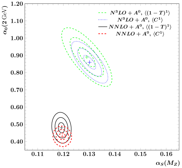
Figure 4: The values of $\alpha_{S}(M_{Z})$ and $\alpha_{0}(2{\,\text{Ge}\kern-0.66666pt\text{V\/}})$ obtained from the NNLO and N³LO fits with analytic hadronization model in the $\mathcal{A}^{0}$ scheme. The contours correspond to $1$-, $2$- and $3$ standard deviations obtained in the fit. Systematic uncertainties are not included.

At the same time, the discrepancy between results obtained with the MC hadronization model and the analytic hadronization model remains in place at N³LO accuracy. This suggests that the discrepancy pattern has a fundamental origin and would hold even in future analyses, regardless of the availability of the exact N³LO predictions. Consequently, the improvement of the hadronization modeling and a better understanding of hadronization itself is more important for increasing the precision of $\alpha_{S}(M_{Z})$ extractions than the calculation of perturbative corrections beyond NNLO. In order to achieve this better understanding and improved modeling of hadronization, in the future it would be important to perform dedicated studies using observables strongly affected by hadronization, e.g. measurements of the hadronic final state in future $e^{+}e^{-}$ experiments at $\sqrt{s}\approx 20-50{\,\text{Ge}\kern-0.66666pt\text{V\/}}$ performed with radiative events or in dedicated collider runs.

7 Conclusions

The aim of the present analysis was to assess the factors that will determine the precision of QCD analyses of $e^{+}e^{-}$ data after the recent and foreseen rapid developments of QCD calculation techniques and the appearance of even more precise theoretical predictions. To do this, we have performed an extraction of the strong coupling $\alpha_{S}(M_{Z})$ from the averages of event shapes event shape moments $\langle(1-T)^{1}\rangle$ and $\langle C^{1}\rangle$ and found that the results obtained using NNLO predictions and analytic hadronization corrections based on the dispersive model are consistent with the last PDG average $\alpha(M_{Z})_{\rm PDG2020}=0.1179\pm 0.0010$.

Furthermore, we considered a method for extracting $\alpha_{S}(M_{Z})$ at N³LO precision in perturbative QCD, employing exact NNLO predictions and estimations of the N³LO corrections from the data. The method produced results which are compatible with the current world average within the somewhat large uncertainties, e.g.

$$\alpha_{S}(M_{Z})^{N^{3}LO+A^{0}}=0.12911\pm 0.00177{\text{(}exp.)}\pm 0.0123{\text{(}scale)}$$

from the $\langle(1-T)^{1}\rangle$ data. The obtained precision can be increased with more high-quality data from future experiments. For the extraction, Monte Carlo and analytic hadronization models were used, the latter being extended to N³LO for the first time. The comparison of the results for these models suggests that extractions of $\alpha_{S}(M_{Z})$ in future analyses will be strongly affected by the modeling of hadronization effects even when the exact higher-order corrections will be included. However, the improvements in the modeling of high-energy physics phenomena by MCEG in the recent decades were closely tied to the experimental measurements performed at the LEP, HERA and LHC colliders and therefore had limited impact on the description of phenomena at lower energies. As a consequence, the advances in modeling of particle collisions at lower energies and understanding of hadronization can be expected only with the availability of new measurements in the corresponding energy ranges.

Appendix A Perturbative coefficients $A_{\mathrm{tot}}$, $B_{\mathrm{tot}}$ and $C_{\mathrm{tot}}$

In this appendix, we recall the total cross section, $\sigma_{\mathrm{tot}}$, of electron-positron annihilation into hadrons. In massless QCD with $N_{F}$ number of light flavors we have [13],

$$\sigma_{\mathrm{tot}}=\sigma_{0}\left[1+\left(\frac{\alpha_{S}}{2\pi}\right)^{1}A_{\mathrm{tot}}\right. +\left(\frac{\alpha_{S}}{2\pi}\right)^{2}B_{\mathrm{tot}}+\left.\left(\frac{\alpha_{S}}{2\pi}\right)^{3}C_{\mathrm{tot}}+\mathcal{O}(\alpha_{S}^{4})\right]\,,$$ (7)

with

$$A_{\mathrm{tot}} =\frac{3}{2}C_{F}\,,$$

$$B_{\mathrm{tot}} =C_{F}\left[\left(\frac{123}{8}-11\zeta_{3}\right)C_{A}-\frac{3}{8}C_{F}-\left(\frac{11}{4}-2\zeta_{3}\right)N_{F}\right]\,,$$

$$C_{\mathrm{tot}} =C_{F}\bigg{[}\left(\frac{90445}{432}-\frac{2737}{18}\zeta_{3}-\frac{55}{3}\zeta_{5}\right)C_{A}^{2}-\left(\frac{127}{8}+\frac{143}{2}\zeta_{3}-110\zeta_{5}\right)C_{A}C_{F}-\frac{69}{16}C_{F}^{2}$$

$$-\left(\frac{1940}{27}-\frac{448}{9}\zeta_{3}-\frac{10}{3}\zeta_{5}\right)C_{A}N_{F}-\left(\frac{29}{16}-19\zeta_{3}+20\zeta_{5}\right)C_{F}N_{F}$$

$$+\left(\frac{151}{27}-\frac{38}{9}\zeta_{3}\right)N_{F}^{2}-\frac{\pi^{2}}{8}\left(\frac{11}{3}C_{A}-\frac{2}{3}N_{F}\right)^{2}\bigg{]}+\frac{(\sum Q_{f})^{2}}{3\sum Q_{f}^{2}}\frac{d^{abc}d^{abc}}{16}\left(\frac{22}{3}-16\zeta_{3}\right)\,.$$

We recall that we use $T_{R}=1/2$ and so $C_{A}=N_{c}=3$, $C_{F}=(N_{c}^{2}-1)/(2N_{c})=4/3$ and $d^{abc}d^{abc}=40/3$. Furthermore, $Q_{f}$ denotes the electric charge of quarks and $N_{F}$ is the number of light quark flavors.

Appendix B Analytic calculations of the perturbative coefficients for the event shape moments

The LO analytic results for $\langle(1-T)^{n}\rangle$, i.e. $A_{0}^{\langle(1-T)^{n}\rangle}$ use the calculations from Ref. [60] and read

$$A_{0}^{\langle(1-T)^{1}\rangle} =C_{F}\left(-\frac{3}{4}\ln(3)-\frac{1}{18}+\frac{\pi^{2}}{3}+4\mathrm{Li}_{2}(3/2)+2\ln(2)^{2}\right)=2.1034701\ldots,$$

$$A_{0}^{\langle(1-T)^{2}\rangle} =C_{F}\left(-\frac{9}{4}\ln(3)+\frac{17}{108}+\frac{\pi^{2}}{3}+4\mathrm{Li}_{2}(3/2)+2\ln(2)^{2}\right)=0.1901961\ldots,$$

$$A_{0}^{\langle(1-T)^{3}\rangle} =C_{F}\left(-\frac{83}{32}\ln(3)+\frac{56}{135}+\frac{\pi^{2}}{3}+4\mathrm{Li}_{2}(3/2)+2\ln(2)^{2}\right)=0.0298753\ldots,$$

$$A_{0}^{\langle(1-T)^{4}\rangle} =C_{F}\left(-\frac{649}{240}\ln(3)+\frac{1259}{2430}+\frac{\pi^{2}}{3}+4\mathrm{Li}_{2}(3/2)+2\ln(2)^{2}\right)=0.0058581\ldots,$$

$$A_{0}^{\langle(1-T)^{5}\rangle} =C_{F}\left(-\frac{527}{192}\ln(3)+\frac{45667}{81648}+\frac{\pi^{2}}{3}+4\mathrm{Li}_{2}(3/2)+2\ln(2)^{2}\right)=0.0012947\ldots,$$

The analytic result for $A_{0}^{\langle C^{1}\rangle}$ has been known for a long time [61]. This result, same as the results for the higher moments can be also obtained with a direct integration, e.g. using the calculations from Ref. [62]. These read:

$$A_{0}^{\langle C^{1}\rangle} =C_{F}\left(-33+4\pi^{2}\right)=8.6378901\ldots\,,$$

$$A_{0}^{\langle C^{2}\rangle} =C_{F}\left(594-60\pi^{2}\right)=2.4316479\ldots\,,$$

$$A_{0}^{\langle C^{3}\rangle} =C_{F}\left(-6750+684\pi^{2}\right)=1.0792137\ldots\,,$$

$$A_{0}^{\langle C^{4}\rangle} =C_{F}\left(65088-\frac{26379}{4}\pi^{2}\right)=0.5685012\ldots\,,$$

$$A_{0}^{\langle C^{5}\rangle} =C_{F}\left(-570024+\frac{1848177}{32}\pi^{2}\right)=0.327216\ldots\,,$$

The NLO coefficient $B_{0}^{\langle C^{1}\rangle}$ was calculated for the first time using the analytic expression for the energy-energy correlations (EEC) from Ref. [63] and the identity on the event level $\langle C^{1}\rangle=\frac{3}{2}\int^{1}_{-1}EEC(\theta)\sin^{2}{\theta}d(cos\theta)$ and we find:

$$B_{0}^{\langle C^{1}\rangle} =C_{F}N_{F}T_{R}\left(\frac{18759}{140}-7\pi^{2}-\frac{2728\zeta_{3}}{35}\right)+C_{F}^{2}\left(-\frac{8947}{224}+\frac{101\pi^{2}}{24}+\frac{2\pi^{4}}{15}-\frac{201\zeta_{3}}{7}\right)$$

$$+C_{A}C_{F}\left(-\frac{209821}{840}+\frac{247\pi^{2}}{18}-\frac{8\pi^{4}}{15}+\frac{7057\zeta_{3}}{35}\right)=172.85901\ldots\,.$$

The results that account for non-zero quark masses are not known analytically even at LO, however the coefficient $A^{\langle C^{1}\rangle}_{m_{b}\neq 0}$ could be derived in a closed from using the results for $EEC_{m_{b}\neq 0}$ from Refs. [64, 65] or the results for the $\frac{dC}{d\sigma}\big{|}_{m_{b}\neq 0}$ from Ref. [62].

Appendix C The $K$, $L$ and $M$ coefficients in different schemes

The $K$, $L$ and $M$ coefficients in the cusp-scheme are simply given by the one-, two- and three-loop cusp anomalous dimensions (for quarks) and read [66, 67, 68, 69, 70, 71]:

$$K_{\mathrm{cusp}} =C_{A}\bigg{(}\frac{67}{18}-\frac{\pi^{2}}{6}\bigg{)}-\frac{5}{9}N_{F},$$

$$L_{\mathrm{cusp}} =C^{2}_{A}\bigg{(}\frac{245}{24}-\frac{67\pi^{2}}{54}+\frac{11\zeta_{3}}{6}+\frac{11\pi^{4}}{180}\bigg{)}+C_{F}N_{F}\bigg{(}-\frac{55}{24}+2\zeta_{3}\bigg{)}$$

$$+C_{A}N_{F}\bigg{(}-\frac{209}{108}+\frac{5\pi^{2}}{27}-\frac{7\zeta_{3}}{3}\bigg{)}-\frac{1}{27}N^{2}_{F},$$

$$M_{\mathrm{cusp}} =\frac{3}{128}(20702-5171.9N_{F}+195.5772N_{F}^{2}+3.272344N_{F}^{3}).$$

The $K$, $L$ and $M$ coefficients in the $\mathcal{A}_{0}$-scheme read [43, 44]:

$$K_{0} =K_{\mathrm{cusp}},$$

$$L_{0} =L_{\mathrm{cusp}}+C_{A}^{2}\left(\frac{77\zeta_{3}}{6}-\frac{1111}{81}\right)+C_{A}N_{F}\left(-\frac{11\pi^{2}}{27}+\frac{356}{81}-\frac{7\zeta_{3}}{3}\right)+N_{F}^{2}\left(\frac{\pi^{2}}{27}-\frac{28}{81}\right),$$

$$M_{0} =M_{\mathrm{cusp}}+C_{A}^{3}\left(\frac{121\pi^{2}\zeta_{3}}{26}-\frac{21755\zeta_{3}}{108}+66\zeta_{5}+\frac{847\pi^{4}}{2160}\right.\left.-\frac{41525\pi^{2}}{1944}+\frac{3761815}{23328}\right)$$

$$+C_{A}^{2}N_{F}\left(-\frac{11\pi^{2}\zeta_{3}}{18}+\frac{6407\zeta_{3}}{108}\right.\left.-12\zeta_{5}-\frac{11\pi^{4}}{54}+\frac{9605\pi^{2}}{972}-\frac{15593}{243}\right)$$

$$+C_{A}C_{F}N_{F}\left(\frac{136\zeta_{3}}{9}+\frac{11\pi^{4}}{180}+\frac{55\pi^{2}}{72}-\frac{7351}{288}\right)$$

$$+C_{A}N_{F}^{2}\left(-\frac{179\zeta_{3}}{54}+\frac{13\pi^{4}}{540}-\frac{695\pi^{2}}{486}+\frac{13819}{1944}\right)$$

$$+C_{F}N_{F}^{2}\left(-\frac{19\zeta_{3}}{9}-\frac{\pi^{4}}{90}-\frac{5\pi^{2}}{36}+\frac{215}{48}\right)+N_{F}^{3}\left(-\frac{2\zeta_{3}}{27}+\frac{5\pi^{2}}{81}-\frac{116}{729}\right),$$

The $K$, $L$ and $M$ coefficients in the $\mathcal{A}_{T}$-scheme read [44]:

$$K_{T} =K_{\mathrm{cusp}},$$

$$L_{T} =L_{\mathrm{cusp}}+C_{A}^{2}\left(\frac{77\zeta_{3}}{6}-\frac{111}{81}\right)-C_{A}N_{F}\left(\frac{7\zeta_{3}}{3}-\frac{356}{81}\right)-\frac{28}{81}N_{F}^{2}.$$

We remind the reader that the complete expression for $M$ is currently not known in the $\mathcal{A}_{T}$-scheme, hence as an approximation, we set $M_{T}=M_{0}$ in this analysis. However, we hope that in the future it will be possible to extend the calculations in the Ref. [44] to higher orders and calculate the $M_{T}$ explicitly.

10

References

- [1] A. Gehrmann-De Ridder et al., NNLO corrections to event shapes in annihilation. JHEP 12, 094 (2007). arXiv:0711.4711
- [2] A. Gehrmann-De Ridder et al., NNLO moments of event shapes in annihilation. JHEP 05, 106 (2009). arXiv:0903.4658
- [3] S. Weinzierl, Event shapes and jet rates in electron-positron annihilation at NNLO. JHEP 06, 041 (2009). arXiv:0904.1077
- [4] S. Weinzierl, Moments of event shapes in electron-positron annihilation at NNLO. Phys. Rev. D80, 094018 (2009). arXiv:0909.5056
- [5] V. Del Duca et al., Three-jet production in electron-positron collisions at next-to-next-to-leading order accuracy. Phys. Rev. Lett. 117, 152004 (2016). arXiv:1603.08927
- [6] V. Del Duca et al., Jet production in the CoLoRFulNNLO method: event shapes in electron-positron collisions. Phys. Rev. D94, 074019 (2016). arXiv:1606.03453
- [7] L.J. Dixon and A. Signer, Electron-positron annihilation into four jets at next-to-leading order in . Phys. Rev. Lett. 78, 811 (1997). arXiv:hep-ph/9609460
- [8] L.J. Dixon and A. Signer, Complete results for . Phys. Rev. D 56, 4031 (1997). arXiv:hep-ph/9706285
- [9] Z. Nagy and Z. Trocsanyi, Next-to-leading order calculation of four jet shape variables. Phys. Rev. Lett. 79, 3604 (1997). arXiv:hep-ph/9707309
- [10] Z. Nagy and Z. Trocsanyi, Next-to-leading order calculation of four jet observables in electron positron annihilation. Phys. Rev. D 59, 014020 (1999). arXiv:hep-ph/9806317. [Erratum: Phys.Rev.D 62, 099902 (2000)]
- [11] J.M. Campbell, M.A. Cullen and E.W.N. Glover, Four jet event shapes in electron-positron annihilation. Eur. Phys. J. C 9, 245 (1999). arXiv:hep-ph/9809429
- [12] S. Weinzierl and D.A. Kosower, QCD corrections to four jet production and three jet structure in annihilation. Phys. Rev. D 60, 054028 (1999). arXiv:hep-ph/9901277
- [13] P.A. Baikov et al., Adler Function, Sum Rules and Crewther Relation of Order : the Singlet Case. Phys. Lett. B714, 62 (2012). arXiv:1206.1288
- [14] R. Frederix et al., NLO QCD corrections to five-jet production at LEP and the extraction of . JHEP 11, 050 (2010). arXiv:1008.5313
- [15] S. Becker et al., NLO results for five, six and seven jets in electron-positron annihilation. Phys. Rev. Lett. 108, 032005 (2012). arXiv:1111.1733
- [16] S. Brandt et al., The principal axis of jets. An attempt to analyze high-energy collisions as two-body processes. Phys. Lett. 12, 57 (1964)
- [17] E. Farhi, A QCD Test for Jets. Phys. Rev. Lett. 39, 1587 (1977)
- [18] G. Parisi, Super Inclusive Cross-Sections. Phys. Lett. B 74, 65 (1978)
- [19] J.F. Donoghue, F.E. Low and So-Young Pi, Tensor Analysis of Hadronic Jets in Quantum Chromodynamics. Phys. Rev. D 20, 2759 (1979)
- [20] G. Somogyi, Z. Trócsányi and V. Del Duca, A Subtraction scheme for computing QCD jet cross sections at NNLO: Regularization of doubly-real emissions. JHEP 01, 070 (2007). arXiv:hep-ph/0609042
- [21] G. Somogyi and Z. Trócsányi, A Subtraction scheme for computing QCD jet cross sections at NNLO: Regularization of real-virtual emission. JHEP 01, 052 (2007). arXiv:hep-ph/0609043
- [22] P. Nason and C. Oleari, Next-to-leading order corrections to momentum correlations in . Phys. Lett. B407, 57 (1997). arXiv:hep-ph/9705295
- [23] C.J. Pahl, Untersuchung perturbativer und nichtperturbativer Struktur der Momente hadronischer Ereignisformvariablen mit den Experimenten JADE und OPAL, Ph.D. thesis, Munich, Max Planck Inst., 2007
- [24] R. Reinhardt, Energieabhängigkeit von Ereignisobservablen Messungen und Studien zu Potenzreihenkorrekturen und Schemenabhängigkeiten, Ph.D. thesis, Wuppertal U., 2001
- [25] DELPHI Coll., P. Abreu et al., Energy dependence of event shapes and of at LEP-2. Phys. Lett. B456, 322 (1999)
- [26] ALEPH Coll., D. Buskulic et al., Studies of QCD in at and . Z. Phys. C73, 409 (1997)
- [27] ALEPH Coll., D. Buskulic et al., Properties of hadronic decays and test of QCD generators. Z. Phys. C55, 209 (1992)
- [28] ALEPH Coll., A. Heister et al., Studies of QCD at centre-of-mass energies between and . Eur. Phys. J. C35, 457 (2004)
- [29] AMY Coll., Y.K. Li et al., Multi-hadron event properties in annihilation at GeV to 57-GeV. Phys. Rev. D41, 2675 (1990)
- [30] HRS Coll., D. Bender et al., Study of quark fragmentation at : global jet parameters and single particle distributions. Phys. Rev. D31, 1 (1985)
- [31] L3 Coll., B. Adeva et al., Studies of hadronic event structure and comparisons with QCD models at the resonance. Z. Phys. C55, 39 (1992)
- [32] L3 Coll., P. Achard et al., Studies of hadronic event structure in annihilation from to with the L3 detector. Phys. Rept. 399, 71 (2004). arXiv:hep-ex/0406049
- [33] MARK-II Coll., G.S. Abrams et al., First Measurements of Hadronic Decays of the Boson. Phys. Rev. Lett. 63, 1558 (1989)
- [34] A. Petersen et al., Multi-hadronic events at and predictions of QCD models from to . Phys. Rev. D37, 1 (1988)
- [35] TASSO Coll., W. Braunschweig et al., Global Jet Properties at to Center-of-mass Energy in Annihilation. Z. Phys. C47, 187 (1990)
- [36] A. Kardos et al., Precise determination of from a global fit of energy-energy correlation to NNLO+NNLL predictions. Eur. Phys. J. C78, 498 (2018). arXiv:1804.09146
- [37] A. Verbytskyi et al., High precision determination of from a global fit of jet rates. JHEP 08, 129 (2019). arXiv:1902.08158
- [38] T. Gehrmann, M. Jaquier and G. Luisoni, Hadronization effects in event shape moments. Eur. Phys. J. C67, 57 (2010). arXiv:0911.2422
- [39] T. Gehrmann, G. Luisoni and P.F. Monni, Power corrections in the dispersive model for a determination of the strong coupling constant from the thrust distribution. Eur. Phys. J. C73, 2265 (2013). arXiv:1210.6945
- [40] Y.L. Dokshitzer, G. Marchesini and B.R. Webber, Dispersive approach to power behaved contributions in QCD hard processes. Nucl. Phys. B 469, 93 (1996). arXiv:hep-ph/9512336
- [41] Y.L. Dokshitzer and B.R. Webber, Power corrections to event shape distributions. Phys. Lett. B 404, 321 (1997). arXiv:hep-ph/9704298
- [42] Y.L. Dokshitzer et al., On the universality of the Milan factor for power corrections to jet shapes. JHEP 05, 003 (1998). arXiv:hep-ph/9802381
- [43] A. Banfi, B.K. El-Menoufi and P.F. Monni, The Sudakov radiator for jet observables and the soft physical coupling. JHEP 01, 083 (2019). arXiv:1807.11487
- [44] S. Catani, D. De Florian and M. Grazzini, Soft-gluon effective coupling and cusp anomalous dimension. Eur. Phys. J. C 79, 685 (2019). arXiv:1904.10365
- [45] J. Bellm et al., Herwig 7.0/Herwig++ 3.0 release note. Eur. Phys. J. C76, 196 (2016). arXiv:1512.01178
- [46] T. Gleisberg et al., Event generation with SHERPA 1.1. JHEP 02, 007 (2009). arXiv:0811.4622
- [47] J. Alwall et al., MadGraph 5 : Going Beyond. JHEP 06, 128 (2011). arXiv:1106.0522
- [48] F. Cascioli, P. Maierhofer and S. Pozzorini, Scattering Amplitudes with Open Loops. Phys. Rev. Lett. 108, 111601 (2012). arXiv:1111.5206
- [49] B. Andersson et al., Parton Fragmentation and String Dynamics. Phys. Rept. 97, 31 (1983)
- [50] B.R. Webber, A QCD model for jet fragmentation including soft gluon interference. Nucl. Phys. B238, 492 (1984)
- [51] J.C. Winter, F. Krauss and G. Soff, A modified cluster hadronization model. Eur. Phys. J. C36, 381 (2004). arXiv:hep-ph/0311085
- [52] A.H. Hoang, S. Platzer and D. Samitz, On the Cutoff Dependence of the Quark Mass Parameter in Angular Ordered Parton Showers. JHEP 10, 200 (2018). arXiv:1807.06617
- [53] R. Baumeister and S. Weinzierl, Cutoff dependence of the thrust peak position in the dipole shower. (2020). arXiv:2004.01657
- [54] G. Luisoni, P.F. Monni and G.P. Salam, -parameter hadronisation in the symmetric 3-jet limit and impact on fit. (2020). arXiv:2012.00622
- [55] F. James and M. Roos, Minuit: A system for function minimization and analysis of the parameter errors and correlations. Comput.Phys.Commun. 10, 343 (1975)
- [56] F. James and M. Winkler, MINUIT User’s Guide. (2004)
- [57] JADE Coll., J. Schieck et al., Measurement of the strong coupling from the three-jet rate in - annihilation using JADE data. Eur. Phys. J. C73, 2332 (2013). arXiv:1205.3714
- [58] M. Dong et al., CEPC Conceptual Design Report: Volume 2 - Physics & Detector. (2018). arXiv:1811.10545
- [59] FCC Study Group, A. Abada et. al, FCC-: The Lepton Collider. Eur. Phys. J. ST 228, 261 (2019)
- [60] A. De Rujula et al., QCD Predictions for Hadronic Final States in Annihilation. Nucl. Phys. B138, 387 (1978)
- [61] R.K. Ellis, D.A. Ross and A.E. Terrano, The Perturbative Calculation of Jet Structure in Annihilation. Nucl. Phys. B 178, 421 (1981)
- [62] M. Preißer, -Parameter with Massive Quarks, 2014, http://othes.univie.ac.at/34188/1/2014-08-29_0902000.pdf
- [63] L.J. Dixon et al., Analytical Computation of Energy-Energy Correlation at Next-to-Leading Order in QCD. Phys. Rev. Lett. 120, 102001 (2018). arXiv:1801.03219
- [64] K.H. Cho, S.K. Han, and J.K. Kim, Energy-energy correlations in electron positron annihilation: Z boson and heavy quark effects. Nucl. Phys. B233, 161 (1984)
- [65] F. Csikor, Quark mass effects for energy-energy correlations in high-energy annihilation. Phys. Rev. D30, 28 (1984)
- [66] G. Curci, W. Furmanski and R. Petronzio, Evolution of Parton Densities Beyond Leading Order: The Nonsinglet Case. Nucl. Phys. B 175, 27 (1980)
- [67] W. Furmanski and R. Petronzio, Singlet Parton Densities Beyond Leading Order. Phys. Lett. B 97, 437 (1980)
- [68] S. Moch, J.A.M. Vermaseren and A. Vogt, The Three loop splitting functions in QCD: The Nonsinglet case. Nucl. Phys. B 688, 101 (2004). arXiv:hep-ph/0403192
- [69] A. Vogt, S. Moch and J.A.M. Vermaseren, The Three-loop splitting functions in QCD: The Singlet case. Nucl. Phys. B 691, 129 (2004). arXiv:hep-ph/0404111
- [70] S. Moch et al., Four-Loop Non-Singlet Splitting Functions in the Planar Limit and Beyond. JHEP 10, 041 (2017). arXiv:1707.08315
- [71] S. Moch et al., On quartic colour factors in splitting functions and the gluon cusp anomalous dimension. Phys. Lett. B782, 627 (2018). arXiv:1805.09638