Scaling Up Deep Neural Network Optimization for Edge Inference

Abstract

Deep neural networks (DNNs) have been increasingly deployed on and integrated with edge devices, such as mobile phones, drones, robots and wearables. To run DNN inference directly on edge devices (a.k.a. edge inference) with a satisfactory performance, optimizing the DNN design (e.g., network architecture and quantization policy) is crucial. While state-of-the-art DNN designs have leveraged performance predictors to speed up the optimization process, they are device-specific (i.e., each predictor for only one target device) and hence cannot scale well in the presence of extremely diverse edge devices. Moreover, even with performance predictors, the optimizer (e.g., search-based optimization) can still be time-consuming when optimizing DNNs for many different devices. In this work, we propose two approaches to scaling up DNN optimization. In the first approach, we reuse the performance predictors built on a proxy device, and leverage the performance monotonicity to scale up the DNN optimization without re-building performance predictors for each different device. In the second approach, we build scalable performance predictors that can estimate the resulting performance (e.g., inference accuracy/latency/energy) given a DNN-device pair, and use a neural network-based automated optimizer that takes both device features and optimization parameters as input and then directly outputs the optimal DNN design without going through a lengthy optimization process for each individual device.

1 Background and Motivation

Deep neural networks (DNNs) have been increasingly deployed on and integrated with edge devices, such as mobile phones, drones, robots and wearables. Compared to cloud-based inference, running DNN inference directly on edge devices (a.k.a. edge inference) has several major advantages, including being free from the network connection requirement, saving bandwidths and better protecting user privacy as a result of local data processing. For example, it is very common to include one or multiple DNNs in today’s mobile apps [41].

To achieve a satisfactory user experience for edge inference, an appropriate DNN design is needed to optimize a multi-objective performance metric, e.g., good accuracy while keeping the latency and energy consumption low. A complex DNN model involves multi-layer perception with up to billions of parameters, imposing a stringent computational and memory requirement that is often too prohibitive for edge devices. Thus, the DNN models running on an edge device must be judiciously optimized using, e.g., neural architecture search (NAS) and model compression [22, 39, 7, 24, 6, 36, 8].

The DNN design choices we focus on in this work mainly refer to the network architecture and compression scheme (e.g., pruning and quantization policy), which constitute an exponentially large space. Note that the other DNN design parameters, such as learning rate and choice of optimizer for DNN training, can also be included into the proposed framework. For example, if we want to consider learning rate and DNN architecture optimization, the accuracy predictor can take the learning rate and architecture as the input and be trained by using different DNN samples with distinct architectures and learning rates.

Given different design choices, DNN models can exhibit dramatically different performance tradeoffs in terms of various important performance metrics (e.g., accuracy, latency, energy and robustness). In general, there is not a single DNN model that performs Pareto optimally on all edge devices. For example, with the same DNN model in Facebook’s app, the resulting latencies on different devices can vary significantly [41]. Thus, device-aware DNN optimization is mandated [37, 24, 41, 26].

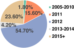
Figure 1: Statistics of the year mobile CPUs are designed as of late 2018 [41].

Designing an optimal DNN for even a single edge device often needs repeated design iterations and is non-trivial [9, 40]. Worse yet, DNN model developers often need to serve extremely diverse edge devices. For example, the DNN-powered voice assistant application developed by a third party can be used by many different edge device vendors, and Facebook’s DNN model for style transfer is run on billions of mobile devices, more than half of which still use CPUs designed in 2012 or before (shown in Fig. 1) [41]. In the mobile market alone, there are thousands of system-on-chips (SoCs) available. Only top 30 SoCs can each take up more than 1% of the share, and they collectively account for 51% of the whole market [41]. Thus, the practice of repeatedly optimizing DNN models, once for each edge device, can no longer meet the demand in view of the extremely diverse edge devices.

Therefore, it has become crucially important to scale up the optimization of DNNs for edge inference using automated approaches.

2 State of the Art and Limitations

Network architecture is a key design choice that affects the resulting performance of DNN models on edge devices. Due to the huge space for network architectures, traditional hand-tuned architecture designs can take months or even longer to train a DNN with a satisfactory performance [42, 15]. Thus, they have become obsolete and been replaced with automated approaches [36]. Nonetheless, the early NAS approaches often require training each DNN candidate (albeit usually on a small proxy dataset), which hence still results in a high complexity and search time. To address this issue, DNN optimization and training need to be decoupled. For example, the current “once-for-all” technique can generate nearly unlimited ($>10^{19}$) DNN models of different architectures all at once [7]. Consequently, DNN model developers can now focus on the optimization of network architecture, without having to train a DNN for each candidate architecture. Thus, instead of DNN training, we consider on scalability of optimizing DNN designs with a focus on the neural architecture.

NAS on a single target device cannot result in the optimal DNN model for all other devices, motivating device-aware NAS. In general, the device-aware NAS process is guided by an objective function, e.g., $accuracy\_loss+weight_{1}*energy+weight_{2}*latency$. Thus, it is crucial to efficiently evaluate the resulting inference accuracy/latency/energy performance given a DNN candidate [38, 31, 29, 25, 33]. Towards this end, proxy models have been leveraged to calculate latency/energy for each candidate, but they are not very accurate on all devices [40]. Alternatively, actual latency measurement on real devices for each candidate is also considered, but it is time-consuming [36].

More recently, performance predictors or lookup tables have been utilized to assist with NAS (and model compression) [38, 31, 29, 25, 33, 24, 35, 39, 6]: train a machine learning model or build a lookup table to estimate the resulting accuracy/latency/energy performance for a candidate DNN design on the target device. Therefore, by using search techniques aided by performance predictors or lookup tables, an optimal DNN can be identified out of numerous candidates for a target edge device without actually deploying or running each candidate DNN on the device [39, 7].

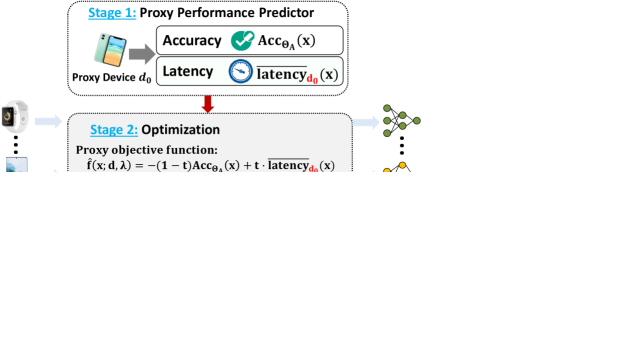
Figure 2: The existing device-aware DNN optimization (i.e., once for a single device) [7, 39, 12].

Nonetheless, as illustrated in Fig. 2, the existing latency/energy predictors or lookup tables [29, 33, 12, 8, 39, 7] are device-specific and only take the DNN features as input to predict the inference latency/energy performance on a particular target device. For example, according to [8], the average inference latencies of 4k randomly selected sample DNNs are measured on a mobile device and then used to train an average latency predictor for that specific device (plus additional 1k samples for testing). Assuming that each measurement takes 30 seconds, it takes a total of 40+ hours to just collect training and testing samples in order to building the latency predictor for one single device, let alone the additional time spent for latency predictor training and other performance predictors. Likewise, to estimate the inference latency, 350K operator-level latency records are profiled to construct a lookup table in [12], which is inevitably time-consuming. Clearly, building performance predictors or lookup tables incurs a significant overhead by itself [29, 33, 12, 8, 39, 7].

More crucially, without taking into account the device features, the resulting performance predictors or lookup tables only provide good predictions for the individual device on which the performance is measured. For example, as shown in Fig. 4 in [12], the same convolution operator can result in dramatically different latencies on two different devices — Samsung S8 with Snapdragon 835 mobile CPU and Hexagon v62 DSP with 800 MHz frequency.

In addition, the optimizer (e.g., a simple evolutionary search-based algorithm or more advanced exploration strategies [33, 31, 25, 29]) to identify an optimal architecture for each device also takes non-negligible time or CPU-hours. For example, even with limited rounds of evolutionary search, 30 minutes to several hours are needed by the DNN optimization process for each device [7, 39, 19]. In [12], the search time may reduce to a few minutes by only searching for similar architectures compared to an already well-designed baseline DNN model, and hence this comes at the expense of very limited search space and possibly missing better DNN designs. Therefore, combined together, the total search cost for edge devices is still non-negligible, especially given the extremely diverse edge devices for which scalability is very important.

There have also been many prior studies on DNN model compression, such as pruning and quantization [14, 22, 23, 17, 10, 18, 1, 11, 30, 27], matrix factorization [13, 28], and knowledge distillation [32], among others. Like the current practice of NAS, the existing optimizer for compression techniques are typically targeting a single device (e.g., optimally deciding the quantization and pruning policy for an individual target device), thus making the overall optimization cost linearly increase with the number of target devices and lacking scalability [39].

In summary, the state-of-the-art device-aware DNN optimization still takes a large amount of time and efforts for even a single device [8, 7, 39, 12], and cannot scale to extremely diverse edge devices.

3 Problem Formulation

A common goal of optimizing DNN designs is to maximize the inference accuracy subject to latency and/or energy constraints on edge devices. Mathematically, this problem can be formulated as

$$\min_{\mathbf{x}\in\mathcal{X}}-accuracy(\mathbf{x})$$ (1)

$$s.t., latency(\mathbf{x};\mathbf{d})\leq\overline{L}_{\mathbf{d}},$$ (3)

$$energy(\mathbf{x};\mathbf{d})\leq\overline{E}_{\mathbf{d}},$$

where $\mathbf{x}$ is the representation of the DNN design choice (e.g., a combination of DNN architecture, quantization, and pruning scheme), $\mathcal{X}$ is the design space under consideration, and $\mathbf{d}$ is the representation of an edge device (e.g., CPU/RAM/GPU/OS configuration). Our problem formulation is not restricted to energy and latency constraints; additional constraints, such as robustness to adversarial samples, can also be added. Note that we use “$-accuracy(\mathbf{x})$” as the objective function to be consistent with the standard “$\min$” operator in optimization problems.

The constrained optimization problem in Eqns. (1)–(3) is called primal problem in the optimization literature [5]. It can also be alternatively formulated as a relaxed problem parameterized by $\lambda=(\lambda_{1},\lambda_{2})$:

$$\min_{\mathbf{x}\in\mathcal{X}}-accuracy(\mathbf{x})+\lambda_{1}\cdot energy(\mathbf{x};\mathbf{d})+\lambda_{2}\cdot latency(\mathbf{x};\mathbf{d}),$$ (4)

where $\lambda=(\lambda_{1},\lambda_{2})$ are non-negative weight parameters (i.e., equivalent to Lagrangian multipliers) corresponding to the energy and latency constraints, respectively. By increasing a weight (say, $\lambda_{2}$ for latency), the optimal design $\mathbf{x}^{*}(\mathbf{d},\lambda)$ by solving (4) will result in better performance corresponding to that weight. If the performance constraint is very loose, then $\lambda=(\lambda_{1},\lambda_{2})$ can approach zero; on the other hand, if the constraint is very stringent, $\lambda=(\lambda_{1},\lambda_{2})$ will be large. Thus, given a set of latency and energy constraints $\overline{L}_{\mathbf{d}}$ and $\overline{E}_{\mathbf{d}}$, we can choose a set of weight parameters $\lambda_{1}$ and $\lambda_{2}$ such that the constraints in (3)(3) are satisfied and the accuracy is maximized.

Strictly speaking, some technical conditions (e.g., convexity) need to be satisfied such that the optimal solution to the relaxed problem in (4) is also the optimal solution to the constrained problem in (1)–(3). Nonetheless, the goal in practice is to obtain a sufficiently good DNN design rather than the truly global optimum, because of the usage of a (non-convex) performance predictor as a substitute of the objective function [7, 8, 24, 39, 12]. Thus, with proper weight parameters $\lambda$, the relaxed version in (4) can be seen as a substitute of the constrained optimization problem (1)–(3).

While the constrained problem formulation in (1)–(3) is intuitive to understand, it may not be straightforward to optimize when using search-based algorithms. On the other hand, when using the relaxed formulation in (4), one needs to find an appropriate set of weight parameters $\lambda=(\lambda_{1},\lambda_{2})$ to meet the performance constraints in (3)(3). In the literature, both constrained and relaxed problems are widely considered to guide optimal DNN designs [39, 12].

In this paper, we choose to solve the relaxed problem in (4) while using efficient searches to identify an optimal $\lambda=(\lambda_{1},\lambda_{2})$ such that the performance constraints in (3)(3) are satisfied and the resulting optimal DNN design $\mathbf{x}$ minimizes the accuracy loss (i.e., maximize the accuracy).

4 Approach 1: Reusing Performance Predictors for Many Devices

A key bottleneck that slows down the DNN optimization process is the high cost of building performance predictors for each device. In our first approach, we propose to reuse the performance predictors built on a proxy device denoted as $\mathbf{d}_{0}$. While the predictor cannot accurately estimate the performance on a different device, it maintains performance monotonicity (e.g., if DNN design $\mathbf{x}_{A}$ has a lower latency than $\mathbf{x}_{B}$ on the proxy device, $\mathbf{x}_{A}$ should still be faster than $\mathbf{x}_{B}$ on a new device) in many cases. We leverage the performance monotonicity to scale up the DNN optimization without re-building performance predictors for each different device.

4.1 Stage 1: Training Performance Predictors on a Proxy Device

To speed up the DNN optimization process, we need to quickly evaluate objective function given different DNN designs. Instead of actually measuring the performance for each DNN design candidate (which is time-consuming), we utilize performance predictors. In our example, we have accuracy/latency/energy predictors. Concretely, the accuracy predictor can be a simple Gaussian process model as used in [12] or a neural network, whose input is the DNN design choice represented by $\mathbf{x}$, and it does not depend on the edge device feature $\mathbf{d}$. We denote the trained accuracy predictor by $Acc_{\Theta_{A}}(\mathbf{x})$, where $\Theta_{A}$ is learnt parameter for the predictor.

On the other hand, the latency/energy predictors depend on devices. Here, we train the latency/energy predictors on a proxy device following the existing studies [39, 12]. For example, to build the latency predictor offline, we can measure the latency for each operator in a DNN candidate and then sum up all the involved operators to obtain the total latency. We denote the latency and energy predictors as $\overline{latency}_{\mathbf{d}_{0}}(\mathbf{x})$ and $\overline{energy}_{\mathbf{d}_{0}}(\mathbf{x})$, where the subscript $\mathbf{d}_{0}$ is to stress that the performance predictors are only accurate (in terms of the absolute performance prediction) for the proxy device $\mathbf{d}_{0}$.

Given the latency/energy predictor for an edge device, one can easily follow [39, 12] and adopt an evolutionary search process to obtain the optimal DNN design. Nonetheless, in [12], the performance predictor cannot transfer to a different device, because the latency/energy performance on one device can change dramatically on a different device: [12] directly uses the absolute performance constraints $\overline{L}_{\mathbf{d}}$ and $\overline{E}_{\mathbf{d}}$ in its (modified) objective function and hence needs accurate performance prediction for each individual device. In [39, 7], the weight parameters $\lambda=(\lambda_{1},\lambda_{2})$ are simply treated as hyperparameters. How to tune $\lambda=(\lambda_{1},\lambda_{2})$ to meet the performance constraints for a target device is not specified. Since it aims at making weighted objective function in (4) as close to the true value as possible on a target device, it needs accurate performance prediction for that target device. Thus, performance predictors are needed for each individual device in [39, 7].

Instead of building a latency/energy predictor for each device, we will reuse the predictor for other devices as described in the next subsection.

4.2 Stage 2: Optimizing DNN Designs on New Devices

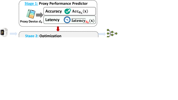
Figure 3: Overview of “reusing performance predictors” to scale up DNN optimization.

In this work, we avoid the cost of building performance predictors for each individual device by leveraging the performance monotonicity of DNNs on different devices. To better explain our idea, we only consider the latency constraint and illustrate our approach in Fig. 3.

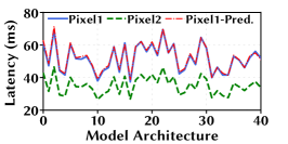
(a) Latencies of 40 DNN models

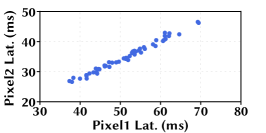
(b) Latency on Pixel 2 vs. Pixel 1

(c) Predicted vs. real latency (Pixel 1)

Figure 4: The measured and predicted average latencies of a set of 40 DNN models with different architectures on Google Pixel 1 and Pixel 2. The latency predictor is built based on Google Pixel 1. The latency values are released accompanying the publication [8].

In many cases, DNNs’ latency performances are monotone on two different devices, which we formally state as follows.

Performance monotonicity. Given two different devices $\mathbf{d}_{0}\not=\mathbf{d}$ and two different DNN designs $\mathbf{x}_{A}\not=\mathbf{x}_{B}$, if $latency(\mathbf{x}_{A};\mathbf{d}_{0})\geq latency(\mathbf{x}_{B};\mathbf{d}_{0})$, then $latency(\mathbf{x}_{A};\mathbf{d})\geq latency(\mathbf{x}_{B};\mathbf{d})$ also holds. We say that the two DNN designs $\mathbf{x}_{A}$ and $\mathbf{x}_{B}$ are performance monotonic on the two devices $\mathbf{d}_{0}$ and $\mathbf{d}$.

Input: Accuracy predictor $Acc_{\Theta_{A}}(\mathbf{x})$, proxy device’s latency predictor $\overline{latency}_{\mathbf{d}_{0}}(\mathbf{x})$, latency constraint on the target device $\overline{L}_{\mathbf{d}}$, already considered $\mathcal{T}$ and corresponding optimal DNN designs $\mathcal{X}^{*}=\{\mathbf{x}^{*}(t),\forall t\in\mathcal{T}\}$, small $\delta>0$ for checking latency constraint satisfaction, and maximum iteration $Max\_Iterate$

Output: Optimal DNN design $\mathbf{x}^{*}$

Initialize: Set $t_{\min}=0$ and $t_{\max}=1$;

for $i$= 1 to $Max\_Iterate$ do

       $t=\frac{t_{\min}+t_{\max}}{2}$;

       if $t\not\in\mathcal{T}$ then

             Solve (6) and obtain $\mathbf{x}^{*}(t)$;

             $\mathcal{T}\leftarrow\mathcal{T}\cup\{t\}$ and $\mathcal{X}^{*}\leftarrow\mathcal{X}^{*}\cup\{\mathbf{x}^{*}(t)\}$

       end if

      Measure latency $latency(\mathbf{x}^{*}(t^{*});\mathbf{d})$;

       if $latency(\mathbf{x}^{*}(t^{*});\mathbf{d})\geq\overline{L}_{\mathbf{d}}+\delta$ then

             $t_{\min}=t$;

       else if $latency(\mathbf{x}^{*}(t^{*});\mathbf{d})\leq\overline{L}_{\mathbf{d}}-\delta$ then

             $t_{\max}=t$;

       else

            Break;

      

end for

return $\mathbf{x}^{*}(t)$;

Algorithm 1 DNN Optimization on a New Device

With performance monotonicity, the relative ranking of different DNNs’ latency performances is preserved between the two devices. For example, as shown in Fig. 4 in [12], for different convolution operators, latency performance monotonicity is observed between Samsung S8 with Snapdragon 835 mobile CPU and Hexagon v62 DSP with 800 MHz frequency, although the absolute performances are very different. We also show in Fig. 4 the performance monotonicity of a set of 40 DNN models with different architectures on Google Pixel 1 and Pixel 2. These two devices have major differences in terms of several specifications, such as operating systems (Android 7.1 vs. Android 8.0), chipset (Qualcomm MSM8996 Snapdragon 821 with 14 nm vs. Qualcomm MSM8998 Snapdragon 835 with 10 nm), CPU (Quad-core 2x2.15 GHz Kryo & 2x1.6 GHz Kryo vs. Octa-core 4x2.35 GHz Kryo & 4x1.9 GHz Kryo) and GPU (Adreno 530 vs Adreno 540), which can affect the latencies. As a result, the absolute latency values on these two devices are very different and not following a simple scaling relation. Nonetheless, on these two devices, many of the DNNs preserve performance monotonicity very well. Moreover, we see that the latency predictor built on Google Pixel 1 is quite accurate compared to the true value. This demonstrates that the latency predictor on Google Pixel 1 can also be reused for Pixel 2, although the authors build another latency predictor for Pixel 2 in their released files [8].

As a result, the latency constraint $latency(\mathbf{x};\mathbf{d})\leq\overline{L}_{\mathbf{d}}$ can be transformed into $latency(\mathbf{x};\mathbf{d}_{0})\leq\overline{L}^{\prime}_{\mathbf{d}}$. That is, there exists another latency constraint $\overline{L}^{\prime}_{\mathbf{d}}$ such that if the latency of a DNN design $\mathbf{x}$ on the proxy device $\mathbf{d}_{0}$ satisfies $latency(\mathbf{x};\mathbf{d}_{0})\leq\overline{L}^{\prime}_{\mathbf{d}}$, then the latency of the same DNN design $\mathbf{x}$ on our target device $\mathbf{d}$ will meet is actual latency constraint, i.e., $latency(\mathbf{x};\mathbf{d})\leq\overline{L}_{\mathbf{d}}$.

Consequently, we convert the original latency constraint $latency(\mathbf{x};\mathbf{d})\leq\overline{L}_{\mathbf{d}}$ into an equivalent latency constraint expressed on the proxy device $latency(\mathbf{x};\mathbf{d}_{0})\leq\overline{L}^{\prime}_{\mathbf{d}}$, which we can reuse the proxy device’s latency predictor to approximate (i.e., $\overline{latency}_{\mathbf{d}_{0}}(\mathbf{x})\leq\overline{L}^{\prime}_{\mathbf{d}}$). Therefore, based on proxy device’s predictor, the DNN design problem for our new target device can be re-written as

$$\min_{\mathbf{x}\in\mathcal{X}}-Acc_{\Theta_{A}}(\mathbf{x}),\;\;\;\;\;s.t.,\;\;\overline{latency}_{\mathbf{d}_{0}}(\mathbf{x})\leq\overline{L}^{\prime}_{\mathbf{d}}.$$ (5)

Nonetheless, without knowing $\overline{L}^{\prime}_{\mathbf{d}}$ a priori, we cannot directly solve the constrained optimization problem (5). Thus, we reformulate the problem (5) as

$$\min_{\mathbf{x}\in\mathcal{X}}-(1-t)\cdot Acc_{\Theta_{A}}(\mathbf{x})+t\cdot\overline{latency}_{\mathbf{d}_{0}}(\mathbf{x}),$$ (6)

where $t\in[0,1]$ plays an equivalent role as $\lambda_{2}$ in the original relaxed problem in (4). With a larger value of $t$, the resulting latency will be smaller (predicted for the proxy device), and vice versa. Importantly, because of performance monotonicity, a larger $t$ will also result in a smaller latency on the new target device. Given each value of $t$, the problem (6) can be quickly solved (e.g., using search-based algorithms), because the objective function can be efficiently evaluated based on accuracy/latency predictors built on the proxy device. For each $t$, there exists a corresponding optimal $\mathbf{x}^{*}(t)$.

Now, the problem reduces to finding an optimal $t^{*}$ such that the actual latency constraint $latency(\mathbf{x};\mathbf{d})\approx\overline{L}_{\mathbf{d}}$ is satisfied and the accuracy is also maximized (i.e., minimizing $-Acc_{\Theta_{A}}(\mathbf{x})$). Then, given $t^{*}$, we can obtain $\mathbf{x}^{*}(t^{*})$. Specifically, for each $t$, we measure the actual latency $latency(\mathbf{x}^{*}(t^{*});\mathbf{d})$ and check if it just meets the actual latency constraint $\overline{L}_{\mathbf{d}}$. Since $t$ is a scalar, we can efficiently search for the optimal $t^{*}$ using bi-section methods. For example, even with a granularity of 0.001 (i.e., 1001 possible values of $t\in[0,1]$), we only need at most $10=\lceil\log_{2}(1001)\rceil$ searches and latency measurements on the target device. This can reduce the significant cost of building a latency predictor for the target device. The algorithm is described in Algorithm 1.

4.3 Remarks

We offer the following remarks on our first approach.

Proxy latency with monotonicity. Essentially, the proxy device’s latency predictor $\overline{latency}_{\mathbf{d}_{0}}(\mathbf{x})$ serves as a proxy latency for the actual target device. Nonetheless, a key novelty and difference from the FLOP-based proxy latency function is that $\overline{latency}_{\mathbf{d}_{0}}(\mathbf{x})$ can preserve performance monotonicity for a large group of devices (i.e., a larger $\overline{latency}_{\mathbf{d}_{0}}(\mathbf{x})$ also means a large actual latency on the target device), whereas FLOP-based proxy latency does not have this desired property and a higher FLOP can commonly have a smaller latency on a target device.

When performance monotonicity does not hold. The core idea of our first approach is to leverage the performance monotonicity of DNNs on different devices. But, this may not hold for all devices: a DNN model with the lowest latency on one device may not always have the best latency performance on another device [26]. The violation of performance monotonicity can be found when the actual latency of a new DNN design becomes significantly higher while it is expected to be lower. If the performance monotonicity does not hold between the proxy device and the new target device, then we will train a new performance predictor for the new target device and treat it as a new proxy device (for possible future reuse); when another device arrives, we will match it with the best suitable proxy devices based on their similarities, and if performance monotonicity does not hold between the new target device and any of the existing proxy devices, we will train a new performance predictor for this new device.

Note that performance monotonicity is not required to strictly hold for all DNNs, as long as it approximately holds for optimal DNN designs $\mathbf{x}^{*}(t)$ for a sufficiently large set of $t$. The reason is that the DNN design problem is non-convex and we only expect to find a reasonably good DNN design, rather than the truly global optimal design. We expect performance monotonicity at least among a group of devices that are not significantly different from each other (e.g., see Fig. 4 for latencies on Google Pixel 1 and Pixel 2, which have different operating systems, chipsets, CPUs and GPUs).

In any case, our approach will not be slower than the existing predictor-aided DNN optimization that requires performance predictors for each different device [12], since our approach can always roll back to the existing approaches by treating each target device as a new proxy device.

Energy constraint. If we also want to factor energy into the objective function, we need to consider a new objective function parameterized by $\mathbf{t}=(t_{1},t_{2})$ where $t_{1}\geq 0$, $t_{2}\geq 0$, and $t_{1}+t_{2}\leq 1$:

$$\min_{\mathbf{x}\in\mathcal{X}}-(1-t_{1}-t_{2})\cdot Acc_{\Theta_{A}}(\mathbf{x})+t_{1}\cdot\overline{latency}_{\mathbf{d}_{0}}(\mathbf{x})+t_{2}\cdot\overline{energy}_{\mathbf{d}_{0}}(\mathbf{x}),$$ (7)

where $\overline{energy}_{\mathbf{d}_{0}}(\mathbf{x})$ is the proxy device’s energy predictor. Accordingly, we need to extend Algorithm 1 to consider a search process over $t_{1}$ and $t_{2}$. While this is more complicated than bi-section on a scalar value, there exist efficient search methods over a multi-dimension space [16]. Regardless, searching over a low-dimensional parameter space $(t_{1},t_{2})$ is much easier than searching over the DNN design space (e.g., architecture space).

5 Approach 2: Learning to Optimize

5.1 Overview

While our first approach aims at avoiding training performance predictors for each individual device, we still need to take a small number of actual latency/energy measurements on each target device, because the proxy device’s performance predictor can only provide a relative/ordered performance instead of the absolute performance. To scale up the optimization of DNNs for edge inference and generate an optimal DNN design instantly for each target device, we now present our second approach.

Our key idea is learning to optimize: instead of performing DNN design optimization repeatedly (once for an individual device), we first learn a DNN optimizer from DNN optimization on sample devices, and then apply the learnt DNN optimizer to new unseen devices and directly obtain the optimal DNN design.

More specifically, we take a departure from the existing practice by: (1) leveraging new performance predictors that can estimate the resulting inference latency/energy performance given a DNN-device pair; and (2) using an automated optimizer which takes the device features and optimization parameters as input, and then directly outputs the optimal DNN design. This is illustrated in Fig. 5. Our latency/energy performance predictors take as explicit input both the DNN features and device features, and hence they can output the resulting performance for new unseen devices. Note that appropriate embedding of DNN and device features will be very helpful to facilitate training the performance predictors and DNN optimizer.

Our automated optimizer utilizes a neural network to approximate the optimal DNN design function, and is intended to cut the search time that would otherwise be incurred for each device. The initial overhead of training our performance predictors and optimizer is admittedly higher than the current practice of only training device-specific predictors, but the overall overhead is expected to be significantly lower, considering the extreme diversity of edge devices.

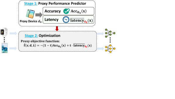
Figure 5: Overview of “learning to optimize” to scale up DNN optimization for edge inference. Once the optimizer is trained, the optimal DNN design for a new device is done almost instantly (i.e., only one inference time).

5.2 Training Performance Predictors and Optimizer

Our proposed design builds on top of two-stage training as described below.

Stage 1: Training performance predictors. The accuracy predictor is the same as the one used in our first approach, since it is measured on a reference dataset without dependence on devices. On the other hand, the latency/energy predictor neural network will use both device feature $\mathbf{d}$ and DNN design representation $\mathbf{x}$ as input, and output the respective performance. They are each trained by running DNNs with sampled designs on training devices and using mean squared error (i.e., the error between the predicted performance and the true measured value) as the loss function. The key difference between our design and [39, 12] is that our latency/energy performance predictors use device features as part of the input and hence can apply to new unseen devices without training new performance predictors.

We denote the set of training edge device features as $\mathcal{D}_{T}^{\prime}$, where each element $\mathbf{d}\in\mathcal{D}_{T}^{\prime}$ corresponds to the feature of one available training device. To generate training samples, we can randomly sample some DNN designs (e.g., randomly select some architectures) plus existing DNN designs if available, and then measure their corresponding performances on training devices as the labels. We denote the trained accuracy/energy/latency predictor neural network by $Acc_{\Theta_{A}}(\mathbf{x})$, $Energy_{\Theta_{E}}(\mathbf{x};\mathbf{d})$, and $Latency_{\Theta_{L}}(\mathbf{x};\mathbf{d})$, respectively, where $\Theta_{A}$, $\Theta_{E}$, and $\Theta_{L}$ are learnt parameters for the three respective networks. Thus, the predicted objective function $\hat{f}(\mathbf{x};\mathbf{d},\lambda)$ can be expressed as

$$\begin{split}\hat{f}(\mathbf{x};\mathbf{d},\lambda)=-Acc_{\Theta_{A}}(\mathbf{x})+\lambda_{1}\cdot Energy_{\Theta_{E}}(\mathbf{x};\mathbf{d})+\lambda_{2}\cdot Latency_{\Theta_{L}}(\mathbf{x};\mathbf{d}).\end{split}$$ (8)

The accuracy/energy/latency predictor neural networks are called performance networks, to be distinguished from the optimizer network we introduce below.

Since collecting energy/latency performances on real training devices is time-consuming, we can use iterative training to achieve better sample efficiency. Specifically, we can first choose a small training set of DNN designs at the beginning, and then iteratively include an exploration set of new DNN designs $\mathcal{X}_{explore}$ to update the performance networks. This is described in Algorithm 2. The crux is how to choose the exploration set $\mathcal{X}_{explore}$. Some prior studies have considered Bayesian optimization to balance exploration vs. exploitation [31, 33], and we leave the choice of $\mathcal{X}_{explore}$ in each iteration as our future work.

Stage 2: Training the automated optimizer. Given an edge device represented by feature $\mathbf{d}$ and optimization parameter $\lambda$, the representation of the corresponding optimal DNN design can be expressed as a function $\mathbf{x}^{*}(\mathbf{d},\lambda)$. The current practice of DNN optimization is to repeatedly run an optimizer (e.g., search-based algorithm), once for a single device, to minimize the predicted objective function [39, 12]. Nonetheless, obtaining $\mathbf{x}^{*}(\mathbf{d},\lambda)$ is non-trivial for each device and not scalable to extremely diverse edge devices. Thus, we address the scalability issue by leveraging the strong prediction power of another fully-connected neural network parameterized by $\Theta$ to approximate the optimal DNN design function $\mathbf{x}^{*}(\mathbf{d},\lambda)$. We call this neural network optimizer network, whose output is denoted by $\hat{\mathbf{x}}_{\Theta}(\mathbf{d},\lambda)$ where $\Theta$ is the network parameter that needs to be learnt. Once $\Theta$ is learnt, when a new device arrives, we can directly predict the corresponding optimal DNN design choice $\hat{\mathbf{x}}_{\Theta}(\mathbf{d},\lambda)$.

For training purposes, in addition to features of real available training devices $\mathcal{D}_{T}^{\prime}$, we can also generate a set of additional synthetic device features $\mathcal{D}_{S}$ to augment the training samples. We denote the combined set of devices for training as $\mathcal{D}_{T}=\mathcal{D}_{T}^{\prime}\cup\mathcal{D}_{S}$, and the training set of optimization parameters as $\Lambda_{T}$ which is chosen according to practical needs (e.g., latency may be more important than energy or vice versa). Next, we discuss two different methods to train the optimizer network.

Input: Real training devices $\mathcal{D}_{T}^{\prime}$, synthetic training devices $\mathcal{D}_{S}$, training set of optimization parameters $\Lambda_{T}$, trained DNN models and their corresponding design space $\mathcal{X}$, initial exploration set of $\mathcal{X}_{explore}$, initial training sets of sampled DNN designs $\mathcal{X}_{T}\subset\mathcal{X}$ and the corresponding accuracy/energy/latency labels measured on real training devices, and maximum iteration rounds $Max\_Iterate$

Output: Performance network parameters $\Theta_{A},\Theta_{E},\Theta_{L}$, and optimizer network parameter $\Theta$

Initialize: Randomize $\Theta_{A},\Theta_{E},\Theta_{L}$, and $\Theta$;

for $i$ = 1 to $Max\_Iterate$ do

       for $\mathbf{x}\in\mathcal{X}_{explore}\subset\mathcal{X}$ and $\mathbf{d}\in\mathcal{D}^{\prime}_{T}$ do

             $\mathcal{X}_{T}\leftarrow\mathcal{X}_{T}\cup\{\mathbf{x}\}$;

             Measure $accuracy(\mathbf{x})$ for a new accuracy label;

             Measure $energy(\mathbf{x};\mathbf{d})$ and $latency(\mathbf{x};\mathbf{d})$ for new energy and latency labels, respectively;

             Update $\Theta_{A},\Theta_{E}$, and $\Theta_{L}$ by training performance networks as described in Stage 1;

       end for

      Choose a new $\mathcal{X}_{explore}$;

      

end for

if Training method 1 is used then

       Fix $\Theta_{A},\Theta_{E},\Theta_{L}$, and obtain $\mathbf{x}^{*}(\mathbf{d},\lambda)=\arg\min_{\mathbf{x}}\hat{f}(\mathbf{x};\mathbf{d},\lambda)$, $\forall(\mathbf{d},\lambda)\in(\mathcal{D}_{T},\Lambda_{T})$;

       Update $\Theta$ by training the optimizer network using Method 1;

else

       Fix $\Theta_{A},\Theta_{E},\Theta_{L}$, and update $\Theta$ by training the optimizer network using Method 2;

return $\Theta_{A},\Theta_{E},\Theta_{L}$, and $\Theta$;

Algorithm 2 Training Performance and Optimizer Networks

Training Method 1: A straightforward method of training the optimizer network is to use the optimal DNN design $\mathbf{x}^{*}(\mathbf{d},\lambda)$ as the ground-truth label for input sample $(\mathbf{d},\lambda)\in(\mathcal{D}_{T},\Lambda_{T})$. Specifically, we can use the mean squared error loss

$$\begin{split}&\min_{\Theta}\frac{1}{N}\sum_{(\mathbf{d},\lambda)\in(\mathcal{D}_{T},\Lambda_{T})}|\hat{\mathbf{x}}_{\Theta}(\mathbf{d},\lambda)-{\mathbf{x}}^{*}(\mathbf{d},\lambda)|^{2}+\mu\|\Theta\|,\end{split}$$ (9)

where $N$ is the total number of training samples, $\mu\|\Theta\|$ is the regularizer to avoid over-fitting, and the ground-truth optimal DNN design $\mathbf{x}^{*}(\mathbf{d},\lambda)$ is obtained by using an existing optimization algorithm (e.g., evolutionary search in [39, 12]) based on the predicted objective function. Concretely, the optimal DNN design used as the ground truth is $\mathbf{x}^{*}(\mathbf{d},\lambda)=\arg\min_{\mathbf{x}}\hat{f}(\mathbf{x};\mathbf{d},\lambda)$, where $\hat{f}(\mathbf{x};\mathbf{d},\lambda)$ is the predicted objective function with parameters $\Theta_{A}$, $\Theta_{E}$, and $\Theta_{L}$ learnt in Stage 1.

Training Method 2: While Method 1 is intuitive, generating many training samples by obtaining the optimal DNN design $\mathbf{x}^{*}(\mathbf{d},\lambda)$, even based on the predicted objective function, can be slow [39, 12]. To reduce the cost of generating training samples, we can directly minimize the predicted objective function $\hat{f}(\mathbf{x};\mathbf{d},\lambda)=-Acc_{\Theta_{A}}(\mathbf{x})+\lambda_{1}\cdot Energy_{\Theta_{E}}(\mathbf{x};\mathbf{d})+\lambda_{2}\cdot Latency_{\Theta_{L}}(\mathbf{x};\mathbf{d})$ in an unsupervised manner, without using the optimal DNN design choice $\mathbf{x}^{*}(\mathbf{d},\lambda)$ as the ground-truth label. Specifically, given the input samples $(\mathbf{d},\lambda)\in(\mathcal{D},\Lambda)$ including both real and synthetic device features, we optimize the optimizer network parameter $\Theta$ to directly minimize the following loss:

$$\begin{split}&\min_{\Theta}\frac{1}{N}\sum_{(\mathbf{d},\lambda)\in(\mathcal{D}_{T},\Lambda_{T})}\hat{f}(\hat{\mathbf{x}}_{\Theta}(\mathbf{d},\lambda);\mathbf{d},\lambda)+\mu\|\Theta\|.\end{split}$$ (10)

The output of the optimizer network directly minimizes the predicted objective function, and hence represents the optimal DNN design. Thus, our training of the optimizer network in Method 2 is guided by the predicted objective function only and unsupervised. When updating the optimizer network parameter $\Theta$, the parameters for performance predictors $\Theta_{A}$, $\Theta_{E}$, and $\Theta_{L}$ learnt in Stage 1 are fixed without updating. In other words, by viewing the concatenation of optimizer network and performance predictor networks as a single neural network (illustrated in Fig. 5), we update the parameters ($\Theta$) in the first few layers while freezing the parameters ($\Theta_{A},\Theta_{E},\Theta_{L}$) in the last few layers to minimize the loss expressed in Eqn. (10).

Finally, we can search for appropriate weight parameters $\lambda$ to obtain the optimal DNN design subject to performance requirement. The key difference between our second approach and the first one is that in the second approach, there is no need to measure the performance for each candidate DNN design on the target device. Note that in our first approach, for each target device, there are only a few candidate DNN designs due to the high efficiency bisection methods.

5.3 Remarks

In this section, we propose a new approach to scaling up DNN optimization for edge inference and present an example of training the optimizer. The key point we would like to highlight in this work is that performing DNN optimization for each individual device as considered in the existing research is not scalable in view of extremely diverse edge devices. We now offer the following remarks (mostly regarding our second approach — learning to optimize).

$\bullet$ DNN update. When a new training dataset is available and the DNN models need to be updated for edge devices, we only need to build a new accuracy predictor on (a subset of) the new dataset and re-train the optimizer network. The average energy/latency predictors remain unchanged, since they are not much affected by training datasets. Thus, the time-consuming part of building energy/latency predictors in our proposed approach is a one-time effort and can be re-used for future tasks.

$\bullet$ Generating optimal DNN design. Once the optimizer network is trained, we can directly generate the optimal DNN design represented by $\hat{\mathbf{x}}_{\Theta}(\mathbf{d},\lambda)$ given a newly arrived edge device $\mathbf{d}$ and optimization parameter $\lambda$. Then, the representation $\hat{\mathbf{x}}_{\Theta}(\mathbf{d},\lambda)$ is mapped to the actual DNN design choice using the learnt decoder. Even though the optimizer network may not always result in the optimal DNN designs for all edge devices, it can at least help us narrow down the DNN design to a much smaller space, over which fine tuning the DNN design becomes much easier than over a large design space.

$\bullet$ Empirical effectiveness. Using performance predictors to guide the optimizer is relevant to optimization from samples [4, 3]. While in theory optimization from samples may result in bad outcomes because the predictors may output values with significant errors, the existing NAS and compression approaches using performance predictors [25, 29, 7, 39, 12] have empirically shown that such optimization from samples work very well and are able to significantly improve DNN designs in the context of DNN optimization. This is partly due to the fact that the predicted objective function only serves as a guide and hence does not need to achieve close to 100% prediction accuracy.

$\bullet$ Relationship to the existing approaches. Our proposed design advances the existing prediction-assisted DNN optimization approaches [39, 12] by making the DNN optimization process scalable to numerous diverse edge devices. If our approach is applied to only one edge device, then it actually reduces to the methods in [39, 12]. Specifically, since the device feature $\mathbf{d}$ is fixed given only one device, we can remove it from our design illustrated in Fig. 5. As a result, our performance predictors are the same as those in [39, 12]. Additionally, our optimizer network can be eliminated, or reduced to a trivial network that has a constant input neuron directly connected to the output layers without any hidden layers. Thus, when there is only one edge device, our approach is essentially identical to those in [39, 12]. Therefore, even in the worst event that the optimizer network or performance predictor network does not generalize well to some new unseen edge devices (due to, e.g., poor training and/or lack of edge device samples), we can always optimize the DNN design for each individual device, one at a time, and roll back to state of the art [39, 12] without additional penalties.

$\bullet$ When scalability is not needed. It has been widely recognized that a single DNN model cannot perform the best on many devices, and device-aware DNN optimization is crucial [39, 7, 12, 37, 41]. Thus, we focus on the scalability of DNN optimization for extremely diverse edge devices. On the other hand, if there are only a few target devices (e.g., a vendor develops its own specialized DNN model for only a few products), our second approach does not apply while our first appraoch (i.e., re-using proxy device’s performance predictors is more suitable).

$\bullet$ GAN-based DNN design. There have been recent attempts to reduce the DNN design space by training generative adversarial networks [20]. Nonetheless, they only produce DNN design candidates that are more likely to satisfy the accuracy requirement, and do not perform energy or latency optimization for DNN designs. Thus, a scalable performance evaluator is still needed to identify an optimal DNN design for diverse edge devices. By contrast, our second approach is inspired by “learning to optimize” [2]: our optimizer network takes almost no time (i.e., only one optimizer network inference) to directly produce an optimal DNN design, and can also produce multiple optimal DNN designs by varying the optimization parameter $\lambda$ to achieve different performance tradeoffs.

$\bullet$ Ensemble. To mitigate potentially bad predictions produced by our optimizer or performance networks, we can use an ensemble in our second approach. For example, an ensemble of latency predictors can be used to smooth the latency prediction, while an ensemble of the optimizer network can be used to generate multiple optimal DNN designs, out of which we select the best one based on (an ensemble of) performance predictors.

$\bullet$ Learning to optimize. Our proposed optimizer network is relevant to the concept of learning to optimize [2], but employs a different loss function in Method 2 which does not utilize ground-truth optimal DNN designs as labels. The recent study [21] considers related unsupervised learning to find optimal power allocation in an orthogonal problem context of multi-user wireless networks, but the performance is evaluated based on theoretical formulas. By contrast, we leverage performance predictors to guide the training of our optimizer network and use iterative training.

$\bullet$ Public datasets for future research. Finally, the lack of access to many diverse edge devices is a practical challenge that prohibits many researchers from studying or experimenting scalable DNN optimization for edge inference. While there are large datasets available on $(architecture,accuracy)$ [34], to our knowledge, there do not exist similar publicly-available datasets containing $(architecture,energy,latency,device)$ for a wide variety of devices. If such datasets can be made available, they will tremendously help researchers build novel automated optimizers to scale up the DNN optimization for heterogeneous edge devices, benefiting every stakeholder in edge inference be it a gigantic player or a small start-up.

References

- [1] Manoj Alwani, Han Chen, Michael Ferdman, and Peter Milder. Fused-layer cnn accelerators. In MICRO, 2016.
- [2] Marcin Andrychowicz, Misha Denil, Sergio Gomez, Matthew W Hoffman, David Pfau, Tom Schaul, Brendan Shillingford, and Nando De Freitas. Learning to learn by gradient descent by gradient descent. In NIPS, 2016.
- [3] Eric Balkanski, Aviad Rubinstein, and Yaron Singer. The power of optimization from samples. In NIPS, 2016.
- [4] Eric Balkanski, Aviad Rubinstein, and Yaron Singer. The limitations of optimization from samples. In STOC, 2017.
- [5] S. Boyd and L. Vandenberghe. Convex Optimization. Cambridge University Press, 2004.
- [6] Ermao Cai, Da-Cheng Juan, Dimitrios Stamoulis, and Diana Marculescu. NeuralPower: Predict and deploy energy-efficient convolutional neural networks. In ACML, 2017.
- [7] Han Cai, Chuang Gan, and Song Han. Once for all: Train one network and specialize it for efficient deployment. In ICLR, 2019.
- [8] Han Cai, Ligeng Zhu, and Song Han. ProxylessNas: Direct neural architecture search on target task and hardware. In ICLR, 2019.
- [9] Hsin-Pai Cheng, Tunhou Zhang, Yukun Yang, Feng Yan, Harris Teague, Yiran Chen, and Hai Li. MSNet: Structural wired neural architecture search for internet of things. In ICCV Workshop, 2019.
- [10] Yu Cheng, Duo Wang, Pan Zhou, and Tao Zhang. A survey of model compression and acceleration for deep neural networks. 2017. Available at: https://arxiv.org/abs/1710.09282.
- [11] Matthieu Courbariaux, Yoshua Bengio, and Jean-Pierre David. Binaryconnect: Training deep neural networks with binary weights during propagations. In NeurIPS, 2015.
- [12] Xiaoliang Dai, Peizhao Zhang, Bichen Wu, Hongxu Yin, Fei Sun, Yanghan Wang, Marat Dukhan, Yunqing Hu, Yiming Wu, Yangqing Jia, et al. ChamNet: Towards efficient network design through platform-aware model adaptation. In CVPR, 2019.
- [13] Emily L Denton, Wojciech Zaremba, Joan Bruna, Yann LeCun, and Rob Fergus. Exploiting linear structure within convolutional networks for efficient evaluation. In NeurIPS, 2014.
- [14] Caiwen Ding, Siyu Liao, Yanzhi Wang, Zhe Li, Ning Liu, Youwei Zhuo, Chao Wang, Xuehai Qian, Yu Bai, Geng Yuan, Xiaolong Ma, Yipeng Zhang, Jian Tang, Qinru Qiu, Xue Lin, and Bo Yuan. CirCNN: Accelerating and compressing deep neural networks using block-circulant weight matrices. In MICRO, 2017.
- [15] Thomas Elsken, Jan Hendrik Metzen, and Frank Hutter. Neural architecture search: A survey. Journal of Machine Learning Research, 20(55):1–21, 2019.
- [16] Manuel López Galván. The multivariate bisection algorithm. arXiv preprint arXiv:1702.05542, 2017.
- [17] Song Han, Huizi Mao, and William J. Dally. Deep compression: Compressing deep neural networks with pruning, trained quantization and huffman coding. In ICLR, 2016.
- [18] Song Han, Jeff Pool, John Tran, and William Dally. Learning both weights and connections for efficient neural network. In NeurIPS, 2015.
- [19] Weiwen Jiang, Lei Yang, Sakyasingha Dasgupta, Jingtong Hu, and Yiyu Shi. Standing on the shoulders of giants: Hardware and neural architecture co-search with hot start. IEEE Transactions on Computer-Aided Design of Integrated CIrcuits and Systems, 2020.
- [20] Sheng-Chun Kao, Arun Ramamurthy, and Tushar Krishna. Generative design of hardware-aware dnns, 2020.
- [21] F. Liang, C. Shen, W. Yu, and F. Wu. Towards optimal power control via ensembling deep neural networks. IEEE Transactions on Communications, 68(3):1760–1776, 2020.
- [22] Ning Liu, Xiaolong Ma, Zhiyuan Xu, Yanzhi Wang, Jian Tang, and Jieping Ye. AutoCompress: An automatic dnn structured pruning framework for ultra-high compression rates. In AAAI, 2020.
- [23] Wei Liu, Xiaolong Ma, Sheng Lin, Shihao Wang, Xuehai Qian, Xue Lin, Yanzhi Wang, and Bin Ren. Patdnn: Achieving real-time DNN execution on mobile devices with pattern-based weight pruning. In ASPLOS, 2020.
- [24] Qing Lu, Weiwen Jiang, Xiaowei Xu, Yiyu Shi, and Jingtong Hu. On neural architecture search for resource-constrained hardware platforms. In ICCAD, 2019.
- [25] Renqian Luo, Fei Tian, Tao Qin, Enhong Chen, and Tie-Yan Liu. Neural architecture optimization. In NIPS, 2018.
- [26] Ningning Ma, Xiangyu Zhang, Hai-Tao Zheng, and Jian Sun. Shufflenet v2: Practical guidelines for efficient cnn architecture design. In ECCV, 2018.
- [27] Bradley McDanel, Surat Teerapittayanon, and HT Kung. Embedded binarized neural networks. 2017. Available at: https://arxiv.org/abs/1709.02260.
- [28] Seyed Yahya Nikouei, Yu Chen, Sejun Song, Ronghua Xu, Baek-Young Choi, and Timothy Faughnan. Smart surveillance as an edge network service: From harr-cascade, svm to a lightweight cnn. In CIC, 2018.
- [29] Xuefei Ning, Wenshuo Li, Zixuan Zhou, Tianchen Zhao, Yin Zheng, Shuang Liang, Huazhong Yang, and Yu Wang. A surgery of the neural architecture evaluators. arXiv preprint arXiv:2008.03064, 2020.
- [30] Mohammad Rastegari, Vicente Ordonez, Joseph Redmon, and Ali Farhadi. Xnor-net: Imagenet classification using binary convolutional neural networks. In ECCV, 2016.
- [31] Binxin Ru, Xingchen Wan, Xiaowen Dong, and Michael Osborne. Neural architecture search using bayesian optimisation with weisfeiler-lehman kernel. arXiv preprint arXiv:2006.07556, 2020.
- [32] Ragini Sharma, Saman Biookaghazadeh, Baoxin Li, and Ming Zhao. Are existing knowledge transfer techniques effective for deep learning with edge devices? In EDGE, 2018.
- [33] Han Shi, Renjie Pi, Hang Xu, Zhenguo Li, James T. Kwok, and Tong Zhang. Multi-objective neural srchitecture search via predictive network performance optimization. arXiv preprint arXiv:1911.09336, 2019.
- [34] Julien Siems, Lucas Zimmer, Arber Zela, Jovita Lukasik, Margret Keuper, and Frank Hutter. NAS-Bench-301 and the case for surrogate benchmarks for neural architecture search. arXiv preprint arXiv:2008.09777, 2020.
- [35] D. Stamoulis, E. Cai, D. Juan, and D. Marculescu. HyperPower: Power- and memory-constrained hyper-parameter optimization for neural networks. In DATE, 2018.
- [36] Mingxing Tan, Bo Chen, Ruoming Pang, Vijay Vasudevan, Mark Sandler, Andrew Howard, and Quoc V Le. MnasNet: Platform-aware neural architecture search for mobile. In CVPR, 2019.
- [37] Hanrui Wang, Zhanghao Wu, Zhijian Liu, Han Cai, Ligeng Zhu, Chuang Gan, and Song Han. HAT: Hardware-aware transformers for efficient natural language processing. In ACL, 2020.
- [38] Linnan Wang, Yiyang Zhao, Yuu Jinnai, Yuandong Tian, and Rodrigo Fonseca. AlphaX: exploring neural architectures with deep neural networks and monte carlo tree search. arXiv preprint arXiv:1903.11059, 2019.
- [39] Tianzhe Wang, Kuan Wang, Han Cai, Ji Lin, Zhijian Liu, Hanrui Wang, Yujun Lin, and Song Han. APQ: Joint search for network architecture, pruning and quantization policy. In CVPR, 2020.
- [40] Bichen Wu, Xiaoliang Dai, Peizhao Zhang, Yanghan Wang, Fei Sun, Yiming Wu, Yuandong Tian, Peter Vajda, Yangqing Jia, and Kurt Keutzer. FBNet: Hardware-aware efficient ConvNet design via differentiable neural architecture search. In CVPR, 2019.
- [41] Carole-Jean Wu, David Brooks, Kevin Chen, Douglas Chen, Sy Choudhury, Marat Dukhan, Kim Hazelwood, Eldad Isaac, Yangqing Jia, Bill Jia, Tommer Leyvand, Hao Lu, Yang Lu, Lin Qiao, Brandon Reagen, Joe Spisak, Fei Sun, Andrew Tulloch, Peter Vajda, Xiaodong Wang, Yanghan Wang, Bram Wasti, Yiming Wu, Ran Xian, Sungjoo Yoo, and Peizhao Zhang. Machine learning at Facebook: Understanding inference at the edge. In HPCA, 2019.
- [42] Barret Zoph and Quoc V Le. Neural architecture search with reinforcement learning. In ICLR, 2017.