A geometric approach to Hu-Washizu variational principle in nonlinear elasticity

Abstract

We discuss the Hu-Washizu (HW) variational principle from a geometric standpoint. The mainstay of the present approach is to treat quantities defined on the co-tangent bundles of reference and deformed configurations as primal. Such a treatment invites compatibility equations so that the base space (configurations of the solid body) could be realised as a subset of an Euclidean space. Cartan’s method of moving frames and the associated structure equations establish this compatibility. Moreover, they permit us to write the metric and connection using 1-forms. With the mathematical machinery provided by differentiable manifolds, we rewrite the deformation gradient and Cauchy-Green deformation tensor in terms of frame and co-frame fields. The geometric understanding of stress as a co-vector valued 2-form fits squarely within our overall program. We also show that for a hyperelastic solid, an equation similar to the Doyle-Erciksen formula may be written for the co-vector part of the stress 2-form. Using this kinetic and kinematic understanding, we rewrite the HW functional in terms of frames and differential forms. Finally, we show that the compatibility of deformation, constitutive rules and equations of equilibrium are obtainable as Euler-Lagrange equations of the HW functional when varied with respect to traction 1-forms, deformation 1-forms and the deformation. This new perspective that involves the notion of kinematic closure precisely explicates the necessary geometrical restrictions on the variational principle, without which the deformed body may not be realized as a subset of the Euclidean space. It also provides a pointer to how these restrictions could be adjusted within a non-Euclidean setting.

Keywords: non-linear elasticity, differential forms, Cartans’ moving frame, kinematic closure, Hu-Washizu variational principle

1 Introduction

Differential forms provide for a natural descriptor of many phenomena of interest in science and engineering [8]. The rules for combining and manipulating differential forms were developed by Hermann Grassmann; however it was only in the work of Élie Cartan that differential forms found a place as a tool to study the geometry of differentiable manifolds. Later, within the broad program of geometrisation of physics, differential forms became an indispensable part in the mathematical description of phenomena. One of the classical examples of a physical theory that was reformulated using differential forms is that of electro-magnetism, where electric and magnetic fields were understood as differential forms of degrees $1$ and $2$ respectively [10]. This reformulation laid bare the key algebraic and geometric features of the theory.

The mechanics of non-linear elastic solids, or the mechanics of continua in general, has a distinctive difference vis-á-vis the theory of electro-magnetism. To be sure, both the theories have sections from the co-tangent bundle or the tensor bundle of the co-tangent space as fields of interest. While electric and magnetic fields are the quantities of interest in electromagnetism, the interest in elasticity is on stresses and strains. The distinction arises from the nature of the base space. In the case of electro-magnetism, the base space is fixed and only sections from the tensor bundle have an evolution rule. In contrast, for an elastic solid the base manifold evolves during the deformation process; such evolutions place restrictions on the evolving sections from the tensor bundle. This additional constraint on sections of the tensor bundle can be overlooked if one chooses to work with deformation as the only variable, when other quantities of interest are derived from it. Such an approach has to an extent been successful for elastic solids. But it suffers from serious drawbacks when one tries to extend the mechanics to inelastic deformation like plasticity, where geometric assumptions on the configuration of a body are brought in to bear on the mechanics [20]. Cavitation in nonlinear elastic solids [4] is another classical example where the deformation alone as the primal variable fails.

It is well understood that the geometry of non-linear elasticity is Eucidean [14]. If one tries to independently evolve stresses and strains along with deformation, one must as well impose the constraint that the configurations of the body are subsets of an Euclidean space. We adopt the method of moving frames proposed by Cartan to achieve this. In this technique, we assign to each point of the configuration, vectors called frame fields. The rate at which these frames vary across the configuration defines the connection 1-forms on the manifold. These connection 1-forms have to satisfy the structure equations so that the parallel transport they encode conforms to the underlying Euclidean structure. Attaching a set of vectors to a material point is not new to the continuum mechanics community. Many such models have been put forth, starting from Cosserat to micromorphic theories; they are often referred to as micro-continuum [7] theories. An important distinction between the present approach and the so called micro-continuum theories is that the latter do not use the directors to encode the connection information. For these models, directors are just degrees of freedom to hold energy. A major trouble with this point of view is that it does not clarify the geometry within which the model is working. An immediate consequence is that the it is impossible to give a co-ordinate independent meaning to the derivatives appearing in the equations of motion. A similar scenario is also encountered in shell theories. Often computational schemes for nonlinear shells [23] are built on models which include directors as degrees of freedom in addition to the mid-surface deformation. We believe that these director degrees of freedom are proxies for the connection induced on the surface. Since these directors do not satisfy any structure equations, it may not be possible to realise these shells as subsets of an Euclidean space.

The goal of this article is to reformulate the kinematics and kinetics of deformation using differential forms. Cartan’s method of moving frames is exploited to construct the kinematics of deformation in terms of frames and co-frames. The kinematic reformulation we propose is a first of its kind and hence not available in the literature. In reformulating the kinetics of deformation, we use the work of Kanso et al. [13], where stress was interpreted as a co-vector valued 2-form. Our kinematic reformulation is also dual to the understanding of stress as a 2-form proposed by Kanso et al.. Using this kinematic-cum-kinetic formalism, we rewrite the HW energy functional and show that it recovers the equilibrium equations as well as compatibility and constitutive rules.

The goals, just stated, have consequences for computation as well. Mixed finite element methods already discussed in the literature may now be realised as tools that place geometry and deformation on an equally important footing. The algebraic and geometric structures brought about by differential forms are instrumental in this. Numerical techniques developed in the form of vector finite elements like the Raviart-Thomas, Nédélec [19, 16, 17] and other carefully handcrafted finite element techniques are now being unified under the common umbrella of finite element exterior calculus, where differential forms play a significant role [5, 3, 2, 11]. Within nonlinear elasticity, techniques based on mixed methods are already the preferred choice [21, 22, 1] for large deformation problems. Motivated by the algebra of differential forms, techniques to approximate differential forms outside the conventional framework of finite elements [12, 25] are also being explored. These techniques can be better developed and interpreted using the geometric approach we propose for the HW functional, when applied to nonlinear elasticity problems.

The rest of the article is organized as follows. A brief introduction to differential forms is given in Section 2. Kinematics of an elastic body is presented in Section 3, where important kinematic quantities like deformation gradient and right Cauchy-Green deformation tensor are reformulated in terms of frame and co-frame fields. This reformulation is facilitated by Cartan’s method of moving frames. This section also contains a discussion on affine connections using connection 1-forms. In Section 4, we introduces stress as a co-vector valued differential 2-form; this interpretation is originally due to Kanso et al.. Then a result like the Doyle-Ericksen formula is presented which yields a constitutive description for traction 1-forms in the presence of a stored energy function. In Section 5, we rewrite the HW variational principle in terms of differential forms using the kinematics and kinetics of deformation developed in Sections 3 and 4. Then we show that variations of the HW functional with respect to different input arguments lead to the compatibility of deformation, constitutive rule and equations of equilibrium. We also remark on the interpretation of stress as a Lagrange multiplier enforcing compatibility of deformation. Finally, in Section 6, we remark on the usefulness of geometrically reformulated HW variational principle in constructing efficient numerical schemes for non-linear elasticity and its extension to other theories in nonlinear solid mechanics.

2 Differential forms in mechanics

We now provide a brief introduction to differential forms; the material is standard and can be found in many introductory texts to differential geometry and manifold theory, e.g. [24, 9]. Let $\mathcal{M}$ be a smooth manifold; at any point of $\mathcal{M}$ one may define the tangent space, which is a vector space. We denote it by $T_{x}\mathcal{M}$. The dual space to this vector space is denote by $T^{*}_{x}\mathcal{M}$. If $\alpha\in T^{*}_{x}\mathcal{M}$ and $v\in T_{x}\mathcal{M}$, then the action $\alpha(v)$ is a real number. The collection of $T_{x}\mathcal{M}$ for each $x\in\mathcal{M}$ is called the tangent bundle $T\mathcal{M}:=\bigcup_{x\in\mathcal{M}}T_{x}\mathcal{M}$; similarly we may define the cotangent bundle as $T^{*}\mathcal{M}=\bigcup_{x\in\mathcal{M}}T^{*}_{x}\mathcal{M}$. If one picks at each point in $\mathcal{M}$ an element of $T^{*}_{x}\mathcal{M}$, we say that a 1-form is defined on $\mathcal{M}$. In other words 1-forms are sections from $T^{*}\mathcal{M}$, just as a vector field is a section from $T\mathcal{M}$. Force is an important example whose differential geometric representation is a 1-form; a force 1-form (or co-vector) acts on a velocity vector to produce power. Electric field is another example which can be represented as a 1-form. Conventionally, in mechanics, the distinction between a 1-form and a vector is ignored allowing one to think of both force and velocity as vectors. This lack of distinction between vectors and 1-forms sacrifices important algebraic and analytical properties pertaining to the exterior algebra, exterior derivatives and integrability of differential forms. In particle mechanics, the integrability of 1-forms (exact forms) translates to the existence of a potential for a force. An alternative and geometric approach to understand $n$-form is to think of them as objects that can be integrated over an orientable $n$ sub-manifold to produce a real number. In other words, an $n$-form is a map from an $n-$dimensional sub-manifold to real numbers. The degree of a differential form is an important property; it is the dimension of the sub-manifold on which the form has to be integrated to produce a real number; it can vary from zero to the dimension of $\mathcal{M}$. The set of all differential forms of degree $n$ over $\mathcal{M}$ is denoted by $\Lambda^{n}(\mathcal{M})$; we may sometimes suppress the argument whenever it is clear where the differential forms are defined. The collection of all $\Lambda^{n}$ over $n$ is denoted by $\Lambda(\mathcal{M})=\bigcup_{i=1,...,n}\Lambda^{i}(\mathcal{M})$. Here $n$ is the dimension of the manifold $\mathcal{M}$. $\Lambda(\mathcal{M})$ is often called the exterior algebra over $\mathcal{M}$.

An important algebraic operation on differential forms is the wedge or skew product. Using the wedge product, one can combine two differential forms to produce a differential form of higher degree. This algebraic operation is denoted by $\wedge$; it is antisymmetric and bilinear. It takes two differential forms of degrees $m$ and $n$ to produce a differential form of degree $m+n$. For any two differential forms $\alpha$ and $\beta$ of degree $m$ and $n$, the wedge product between them satisfies the following anti-symmetric relationship.

$$\alpha\wedge\beta=(-1)^{mn}\beta\wedge\alpha$$ (1)

Let $\mathcal{M}$ and $\mathcal{N}$ be two smooth manifolds and $\varphi$ be a diffeomorphism between them; $\varphi:\mathcal{M}\rightarrow\mathcal{N}$ and $\alpha\in\Lambda^{n}(\mathcal{N})$. The pull back of $\alpha$ to the co-tangent space $T^{*}\mathcal{M}$ is denoted by $\varphi^{*}(\alpha)$ and is given by the following relationship,

$$\varphi^{*}(\alpha)(v^{1},...,v^{n})=\alpha({\text{d}}\varphi v^{1},...,{\text{d}}\varphi v^{n}),\quad v^{i}\in T\mathcal{M}$$ (2)

Here, ${\text{d}}\varphi$ is the differential of $\varphi$; it maps $T\mathcal{M}$ to $T\mathcal{N}$. (2) must be understood as a point-wise relationship at each tangent space of $\mathcal{M}$ and $\varphi(\mathcal{M})$ respectively. Under the pull-back map, the wedge product is distributive. If $\alpha,\beta\in T^{*}\mathcal{N}$, then

$$\varphi^{*}(\alpha\wedge\beta)=\varphi^{*}(\alpha)\wedge\varphi^{*}{\beta}$$ (3)

where $\varphi^{*}(.)$ is defined as in (2).

On a smooth manifold, one can define a notion of differentiation for differential forms called the exterior differentiation. It turns out that this notion of differentiation is coordinate independent. If $\alpha$ is a differential form, then its exterior derivative is denoted by ${\text{d}}\alpha$. The exterior derivative operator is a linear map and increases the degree of a differential form by 1. An important property of the exterior derivative is that ${\text{d}}\circ{\text{d}}=0$; the second exterior derivative of a differential form is identically zero. Under a diffeomorphism, the exterior derivative commutes with its pull back. This relationship may be written as,

$$\varphi^{*}{{\text{d}}\alpha}={\text{d}}(\varphi^{*}\alpha)$$ (4)

Exterior derivative is also distributive when applied to the wedge product of two differential forms. For differential forms $\alpha$ and $\beta$ of degree $n$ and $m$, the exterior derivative of wedge product between them is given by,

$${\text{d}}(\alpha\wedge\beta)={\text{d}}\alpha\wedge\beta+(-1)^{n}\alpha\wedge{\text{d}}\beta$$ (5)

Using exterior differentiation, one can define closed and exact forms. We say that a differential form $\alpha\in\Lambda^{n}$ is exact if there exists a differential form $\beta\in\Lambda^{n-1}$ such that $\alpha={\text{d}}\beta$. The differential form $\alpha$ is closed if ${\text{d}}\alpha=0$. If we assume $\mathcal{M}$ to be a simply connected subset of $\mathbb{R}^{n}$, Poincaré lemma establishes that closed forms are also exact. The failure of a closed form to be exact is measured by the co-homology group. If $\mathcal{C}\subset\mathcal{M}$ is a hyper-surface of dimension $m$ and $\alpha$ is a differential form of degree $m-1$, Stokes theorem relates ${\text{d}}\alpha$ to the trace of $\alpha$ on the boundary of $\mathcal{C}$ denoted by $\partial\mathcal{C}$. Stokes theorem can be written as,

$$\int_{\mathcal{C}}{\text{d}}\alpha=\int_{\partial\mathcal{C}}\alpha$$ (6)

We now assume that the manifold $\mathcal{M}$ is equipped with a metric $g$ and ${\text{d}}\mathsf{V}$ denotes the volume form generated by the metric. In such a case, one can define a linear isomorphism between differential forms of degree $m$ and $n-m$ ($n$ denotes the dimension of $\mathcal{M}$), for each $n$. This isomorphism is defined by the following relationship,

$$\alpha\wedge\beta=\langle{}_{\star}\alpha,\beta\rangle_{g}{\text{d}}\mathsf{V};\quad\alpha\in\Lambda^{n},\beta\in\Lambda^{n-m}$$ (7)

In the above equation, $\langle.,.\rangle_{g}$ is the inner-product induced by the metric on $\Lambda^{n-m}$. This isomorphism is called the Hodge star map; $\star:\Lambda^{m}\rightarrow\Lambda^{n-m}$. It turns out that this map is useful in defining stresses and computing the variation of the HW energy functional.

3 Kinematics

The reference configuration of the body is identified with a smooth manifold with boundary. This manifold is denoted by $\mathcal{B}$ and its boundary by $\partial\mathcal{B}$. Similarly, the deformed configuration and its boundary are denoted by $\mathcal{S}$ and $\mathcal{\partial S}$ respectively. These configurations are endowed with a $C^{\infty}$ chart from which they inherit their smoothness. Following the usual notation in continuum mechanics, we label the material points of the reference and deformed configurations by their position vectors. The position vectors of a material point in the reference and deformed configuration are denoted by $X$ and $x$ with coordinates $X^{i}$ and $x^{i}$. The tangent and co-tangent spaces at each point $X\in\mathcal{B}$ is denoted by $T_{X}\mathcal{B}$ and $T^{*}_{X}\mathcal{B}$ respectively. The deformation map relating the reference and deformed configurations is denoted by $\varphi:\mathcal{B}\rightarrow\mathcal{S}$. The tangent and co-tangent spaces of the deformed configuration at a point $x=\varphi(X)$ is denote by $T_{\varphi(X)}\mathcal{S}$ and $T^{*}_{\varphi(X)}\mathcal{S}$ respectively.

3.1 Frame and co-frame fields

At each tangent space of $\mathcal{B}$, we choose a collection of orthogonal vectors; we denote these vectors by $E_{i}$. Note that the orthogonality here is with respect to the Euclidean inner product. In other words, we have assumed that each tangent space of the reference or deformed configuration is endowed with a metric tensor, which is Euclidean. We call this collection of vector fields a frame field to the reference configuration and it is denoted by $\mathcal{F}_{\mathcal{B}}=\{E_{1},...,E_{n}\}$. It is clear that the frame fields at point $X$ span $T_{X}\mathcal{B}$. Similarly, the orthonormal frame field associated with the deformed configuration is denoted by $\mathcal{F}_{\mathcal{S}}=\{e_{1},...,e_{n}\}$, where $e_{i}$ are sections from $T\mathcal{S}$. The natural (algebraic) duality between tangent and cotangent spaces induces co-frames on the cotangent bundles of $\mathcal{B}$ and $\mathcal{S}$. The co-frames of the reference and deformed configurations are denoted by $\mathcal{F}^{*}_{\mathcal{B}}=\{E^{i},...,E^{n}\}$ and $\mathcal{F}^{*}_{\mathcal{S}}=\{e^{1},...,e^{n}\}$ respectively, where $E^{i}$ and $e^{i}$ are sections from the cotangent bundles of the reference and deformed configurations. The natural duality between frame and co-frame fields of the reference and deformed configurations may be written as,

$$E^{i}(E_{j})=\delta^{i}_{j};\quad e^{i}(e_{j})=\delta^{i}_{j}\quad E^{i}\in T^{*}\mathcal{B},e^{i}\in T^{*}\mathcal{S}$$ (8)

The differential of the position vector of a material point in the reference configuration is denoted by ${\text{d}}X$ and is given by,

$${\text{d}}X=E_{i}\otimes E^{i}$$ (9)

Similarly, the differential of a position vector in the deformed configuration in terms of the frame and co-frame fields is given by,

$${\text{d}}x=e_{i}\otimes e^{i}$$ (10)

From the definition of ${\text{d}}X$ in (9), it can be seen that tangent vectors from the reference configuration are mapped to itself under ${\text{d}}X$. To see this, choose $V\in T_{X}\mathcal{B}$ with $V=c^{i}E_{i}$. Substituting the latter and using the definition of ${\text{d}}X$, we arrive at ${\text{d}}X(V)=c^{j}E_{i}E^{i}(E_{j})$. Using the duality between the frame and co-frame fields, we conclude ${\text{d}}X(V)=V$. Similarly, ${\text{d}}x$ maps a tangent vector from the deformed configuration on to itself. The differential of a position vector in the reference and deformed configurations are thus identity maps on the respective tangent spaces. The importance of the differential of position will be clarified when we discuss deformation gradient.

Similar to the differential to position, one can also define the differential of a frame field. The differential of the frame fields in the reference configuration is given by,

$${\text{d}}E_{i}=\gamma^{j}_{i}\otimes E_{j}$$ (11)

where, $\gamma^{i}_{j}$ is called the connection matrix; it contains 1-forms as its entries. Because of the orthogonality of the frame fields, the connection matrix is skew symmetric, i.e. $\gamma^{i}_{j}=-\gamma^{j}_{i}$. Similarly, the differential of the frame fields associated with the deformed configuration is given by,

$${\text{d}}e_{i}=\bar{\omega}^{j}_{i}\otimes e_{j}$$ (12)

$\bar{\omega}^{i}_{j}$ is the connection matrix associated with the deformed frame fields and it is also skew symmetric, $\bar{\omega}^{i}_{j}=-\bar{\omega}^{j}_{i}$.

For a given choice of connection 1-forms and position 1-forms, there are certain compatibility conditions (Poincaré relations) guaranteeing the existence of position vectors. These equations are called Cartan’s structure equations. The first compatibility condition establishes the torsion free nature of a configuration. For the reference and deformed configurations, this condition may be written as,

$${\text{d}}^{2}{X}=0;\;{\text{d}}^{2}x=0$$ (13)

Plugging (9) and (10) into the above equation leads to,

$${\text{d}}E^{i}=\gamma^{i}_{j}\wedge E^{j};\;{\text{d}}e^{i}=\bar{\omega}^{i}_{j}\wedge e^{j}$$ (14)

The second compatibility condition establishes that the reference and deformed configurations are curvature-free. This leads to the following conditions on the reference and deformed frame fields,

$${\text{d}}^{2}E_{i}=0;\;\;{\text{d}}^{2}e_{i}=0$$ (15)

Using the differential of the frame fields in the above equations leads to,

$${\text{d}}\gamma^{i}_{j}=\gamma^{i}_{k}\wedge\gamma^{k}_{j};\;\;{\text{d}}\bar{\omega}^{i}_{j}=\bar{\omega}^{i}_{k}\wedge\bar{\omega}^{k}_{j}$$ (16)

For a simply connected body, the structure equations as above for the reference and deformed configurations provide the necessary kinematic closure to ensure that the configurations can be embedded with an Euclidean space. Indeed, without this closure effected by the structure equations, a model cannot in general produce a deformed configuration which is Euclidean embeddable.

3.2 Differentials of position and frame

In the previous sub-section, we introduced the notion of differentials to position vectors and frame fields. We now present the geometric meaning of these infinitesimal quantities. Consider the differential of the position vector in the reference configuration given in (9). For a given coordinate system, the position vector $X$ is a smooth function of its coordinates $(X^{1},X^{2},X^{3})$. Let $\Gamma$ be a parametrized curve, $\Gamma:[a,b]\rightarrow\mathcal{B}$. For convenience, we assume $\Gamma$ to be along the first coordinate direction, which is obtained by freezing the other two coordinate functions to some constant. We also assume that the frame fields $E_{i}$ are constructed by a Gram–Schmidt procedure on the tangent vectors of the co-ordinate lines at each material point $X$. Fig. 1 shows how the position vector and the frame change as one moves along the curve $\Gamma$. From our assumptions on $\Gamma$, it may be seen that the tangent vector to $\Gamma$ is given by the $cE_{1}$, where $c$ is a real valued function. Now, the differential of position, which is a vector valued 1-form, can be integrated along the curve $\Gamma$ to produce a vector. This is nothing but the vector between the material points $X(a)$ and $X(b)$, which may be formally written as,

$$X(b)-X(a) =\int_{a}^{b}\text{d}X(cE_{1}){\text{d}}s$$

$$=\int_{a}^{b}cE_{i}E^{i}(E_{1}){\text{d}}s,$$

$$=\int_{a}^{b}cE_{1}{\text{d}}s,$$ (17)

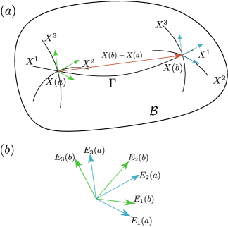
Figure 1: The coordinate lines and the frame field generated from these coordinate lines are shown in (a). The frame fields at $X(a)$ and $X(b)$ are shown in (b); we have moved the frames to the same point so that it is convenient to interpret the change. We have used the notation $E_{i}(a)$ and $E_{i}(b)$ to indicate the frame at the material points $X(a)$ and $X(b)$.

In the above equation, $E_{1}$ and $c$ can vary along the curve $\Gamma$. The above interpretation of ${\text{d}}X$ is very similar to that of 1-forms as real numbers defined on curves.

We now consider the differential of the frame field, integrating which along $\Gamma$ leads to the relative rotation of the frame $\mathcal{F}$ between the points $X(a)$ and $X(b)$. Fig. 1(b) demonstrates the rotation experienced by the frame as one traverses along the curve $\Gamma$.

$$E_{i} =\int_{a}^{b}{\text{d}}E_{i}(E_{1}){\text{d}}s;$$

$$=\int_{a}^{b}E_{j}\gamma^{j}_{i}(E_{1}){\text{d}}s;$$ (18)

From the discussion, it is clear that the displacement (rotation) vector between two points (frames) in a configuration depends on the position 1-form and the curve or path used for integration. However, the displacement vector between two points on a configuration should be independent of the path chosen to integrate the 1-forms. This condition is exactly what the structure equation enforces.

3.3 Deformation gradient

As discussed earlier, the deformation map sends the position vector of a material point in the reference configuration to its corresponding position vector in the deformed configuration. The differential of the deformation map or the deformation gradient, denoted by ${\text{d}}\varphi$, maps the tangent space of the reference configuration to the corresponding tangent space in the deformed configuration. For an assumed frame field (for both reference and deformed configurations), the differential of the deformation map can be obtained by pulling back the co-vector part of the differential of the deformed position vector.

$$\text{d}\varphi =e_{i}\otimes\varphi^{*}(e^{i})$$

$$=e_{i}\otimes\theta^{i};\quad\theta^{i}\in T^{*}\mathcal{B},e_{i}\in\mathcal{F}_{\mathcal{S}}$$ (19)

In writing (19), we have introduced the following definition: $\theta^{i}:=\varphi^{*}({e^{i}})$. In our construction, the 1-forms $\theta^{i}$ contain local information about the deformation map $\varphi$. A primitive variable in our theory, we call this the deformation 1-form. From (19), we see that the vector leg of the deformation gradient is from the deformed configuration, while the co-vector leg is from the reference configuration. If $V(X)\in T_{X}\mathcal{B}$, the action of the deformation gradient on $V$ is given by,

$${\text{d}}\varphi(V)=e_{i}\theta^{i}(V)$$ (20)

Since $\theta^{i}(V)$ are real numbers, the above equation is a linear combination of tangent vectors from the deformed configuration.

3.4 Pull-back of structure equations

Having introduced the deformation gradient and the deformation 1-form in the last subsection, we are now ready to rewrite the referential version of structure equations in the deformed configuration. These equations are obtained by pulling back the structure equations for the deformed configuration under the deformation map:

$$\varphi^{*}({\text{d}}{e^{i}}) =\varphi^{*}(\bar{\omega}^{i}_{j}\wedge e^{j})$$

$${\text{d}}\theta^{i} =\omega^{i}_{j}\wedge\theta^{j}$$ (21)

where, $\omega^{i}_{j}:=\varphi^{*}(\bar{\omega}^{i}_{j})$ are called pulled back connection 1-forms. The key fact used in obtaining the above equation is that exterior derivative and wedge product commute with pull back. Using a similar argument, the pull back of the second compatibility condition is given by,

$${\text{d}}\omega^{i}_{j}=\omega^{i}_{k}\wedge\omega^{k}_{j}$$ (22)

For concreteness, we present the components of the structure equations in three spatial dimensions. Each structure equation constitutes a system of three equations. The matrix form of the first structure equation (referentially pulled back) may be written as,

$$\begin{bmatrix}\text{d}\theta^{1}\\ \text{d}\theta^{2}\\ \text{d}\theta^{3}\\ \end{bmatrix}=\begin{bmatrix}0&\omega^{1}_{2}&-\omega^{1}_{3}\\ -\omega^{1}_{2}&0&-\omega^{2}_{3}\\ \omega^{1}_{3}&\omega^{2}_{3}&0\end{bmatrix}\wedge\begin{bmatrix}\theta^{1}\\ \theta^{2}\\ \theta^{3}\\ \end{bmatrix}$$ (23)

Note that the combining rule for the elements of the matrix and the vector on the right hand side of the above equation is via the wedge product. The component form of the second compatibility equations is given by,

$${\text{d}}\omega^{1}_{3} =\omega^{1}_{2}\wedge\omega^{2}_{3}$$

$${\text{d}}\omega^{2}_{3} =\omega^{1}_{2}\wedge\omega^{1}_{3}$$ (24)

$${\text{d}}\omega^{1}_{2} =\omega^{1}_{3}\wedge\omega^{2}_{3}$$

3.5 Strain and deformation measures

The notion of length is central to continuum mechanics; important kinematic quantities like strain and rate of deformation are derived from it. Indeed, it may not be possible to assess the state of deformation without the metric structure defined on both reference and deformed configurations. The metric structure of a configuration is defined by a symmetric and positive definite tensor, which encodes the notion of length (in that configuration). We denote the metric tensor of the reference and deformed configurations by $G$ and $g$ respectively; $G:T_{X}\mathcal{B}\times T_{X}\mathcal{B}\rightarrow\mathbb{R}$ and $g:T_{x}\mathcal{S}\times T_{x}\mathcal{S}\rightarrow\mathbb{R}$. These tensor valued functions pertain to the idea of infinitesimal lengths at the tangent spaces of $\mathcal{B}$ and $\mathcal{S}$. As such, the notion of length is an additional structure placed on $\mathcal{B}$ and $\mathcal{S}$. In this work, we assume these metrics to be Euclidean. In terms of the co-frame field, the metric tensor of the reference configuration is given as,

$$G =(E^{j}\otimes E_{j}):(E_{i}\otimes E^{i})$$

$$=E^{i}\otimes E^{i}$$ (25)

The double contraction in the above equation is calculated using the inner product induced by the Euclidean metric. Similarly, the metric tensor in the deformed configurations may be written as,

$$g =(e^{i}\otimes e_{j}):(e_{j}\otimes e^{i})$$

$$=e^{i}\otimes e^{i}$$ (26)

In terms of the frame fields, the inverses of the metric tensors for the reference and deformed configurations may be written as,

$$G^{-1}=E_{i}\otimes E_{i};\;\;\;g^{-1}=e_{i}\otimes e_{i}$$ (27)

The right Cauchy-Green deformation tensor is obtained via the pull back of the metric tensor of the deformed configuration to the reference configuration. In terms of the the co-frame fields, this relationship can be written as,

$$C =\varphi^{*}(g)$$

$$=\varphi^{*}(e^{i}\otimes e^{i})$$

$$=\theta^{i}\otimes\theta^{i}$$ (28)

An alternate way to compute the $C$ is to use the usual definition in continuum mechanics, $C=\text{d}\varphi^{t}\text{d}\varphi$. Here, the $(.)^{t}$ is understood to be the adjoint map induced by the metric structure. Using the orthonormality of the frame field we arrive at,

$$C =(\theta^{i}\otimes e^{i})(e_{j}\otimes\theta^{j})$$

$$=\theta^{i}\otimes\theta^{i}$$ (29)

The calculations leading to (28) and (29) are exactly the same; only the sequence in which pull back and inner product are applied differs. The Green-Lagrangian strain tensor may now be written as,

$$E =\frac{1}{2}(C-G)$$

$$=\frac{1}{2}[(\theta^{i}\otimes\theta^{i})-(E^{i}\otimes E^{i})]$$ (30)

The the first invariant of the right Cauchy-Green tensor is given by,

$$I_{1}=\langle\theta^{i},\theta^{i}\rangle_{G}$$ (31)

Here $\langle.,.\rangle_{G}$ denotes the inner product induced by the metric tensor $G$. The area forms induced by the co-frame of the reference configuration are given by,

$${\text{d}}A^{1}=E^{2}\wedge E^{3};\quad{\text{d}}A^{2}=E^{3}\wedge E^{1};\quad{\text{d}}A^{3}=E^{1}\wedge E^{2};\quad$$ (32)

Similarly, the area forms induced by the co-frame of the deformed configurations are given by,

$${\text{d}}a^{1}=e^{2}\wedge e^{3};\quad{\text{d}}a^{2}=e^{3}\wedge e^{1};\quad{\text{d}}a^{3}=e^{1}\wedge e^{2};\quad$$ (33)

We also define the pulled back area forms from those of the deformed configuration to the reference configuration. These area forms are obtained as,

$${\text{d}}\mathsf{A}^{1}=\theta^{2}\wedge\theta^{3};\quad{\text{d}}\mathsf{A}^{2}=\theta^{3}\wedge\theta^{1};\quad{\text{d}}\mathsf{A}^{3}=\theta^{1}\wedge\theta^{2};\quad$$ (34)

In writing the above equations, we have used ${\text{d}}\mathsf{A}^{i}:=\varphi^{*}({\text{d}}a^{i})$ and the definition of the deformation 1-form. The second invariant of $C$ is now given by,

$$I_{2}=\langle{\text{d}}\mathsf{A}^{i},{\text{d}}\mathsf{A}^{i}\rangle_{G}$$ (35)

In terms of co-frame fields, the volume forms of reference and deformed configurations may be written as,

$${\text{d}}V=E^{1}\wedge E^{2}\wedge E^{3};\quad{\text{d}}v=e^{1}\wedge e^{2}\wedge e^{3}$$ (36)

The pull back of ${\text{d}}v$ to the reference configuration is,

$${\text{d}}\mathsf{V}=\theta^{1}\wedge\theta^{2}\wedge\theta^{3}$$ (37)

The third invariant of $C$ is then given by,

$$I_{3}=({}_{\star}{\text{d}}\mathsf{V})^{2}$$ (38)

3.6 Affine connection via frame fields

An affine connection on a smooth manifold is a device used to differentiate sections of vector and tensor bundles in a co-ordinate independent manner. This differentiation is often referred to as covariant. The choice of an affine connection determines the covariant differentiation. For a smooth manifold with a metric, the metric induces a unique covariant derivative and we denote it by $\nabla$. For vector fields $v,w$ and a real valued function $f$, the covariant derivative satisfies the following properties.

$$\nabla_{fe_{i}}w =f\nabla_{e_{i}}w;\;\;f\in\Lambda^{0}$$

$$\nabla_{e_{i}}(w+v) =\nabla_{e_{i}}w+\nabla_{e_{i}}v$$ (39)

$$\nabla_{e_{i}}(fw) =e_{i}[f]w+f\nabla_{e_{i}}w$$

$e_{i}[f]$ in the above equations denotes the action of a vector field on a real valued function $f$. We now show how the connection 1-forms encode the affine connection. Let $w=\sum_{i=1}^{2}w^{i}e_{i}$ is an arbitrary vector field defined on $\mathcal{S}$. Then the covariant derivative of $w$ in the direction of $e_{i}$ is given by,

$$\nabla_{e_{i}}w={\text{d}}w^{j}(e_{i})e_{j}+w^{j}\bar{\omega}^{k}_{j}(e_{i})e_{k}$$ (40)

Having defined the covariant derivative of a vector field in the direction of frame fields, it is now possible to extend the above definition of covariant differentiation to arbitrary vector fields using the defining properties given in (39).

4 Stress as co-vector valued two-form

In the previous section, we have reformulated the kinematics of continua using differential forms. The right Cauchy-Green deformation tensor and the deformation gradient were the key objects in the reformulation. In this section, we present a geometric approach to stress, originally due to Kanso et al. [13]. Even though this approach is intuitive and geometric, it was never put to use. In classical dynamics [15], force is understood as a co-vector so that its pairing with velocity produces power. This understanding of force as dual to velocity does not require the metric tensor to compute power and it must be contrasted with the usual understanding of of both velocity and force as vectors. Extending this concept of force as a co-vector to the continuum mechanical definition of stress is our present goal. As a consequence, we also show that the description of power/work used in continuum mechanics may be undertaken without the notion of a metric. However, it should also be noted that a formulation of continuum mechanics without the metric tensor may not be feasible as the notion of strain crucially depends on the metric.

We denote the Cauchy stress tensor by $\sigma$. The traction ’vector’ acting on an infinitesimal area with unit normal $n$ is denoted by $t$, given by the well known formula $t=\sigma n$. The traction $t$ is a force which depends on the material point at which it is evaluated and the area which sustains it. The relation between the normal and the traction is postulated to be linear. In the language of differential forms, an infinitesimal area is regarded as a 2-form, while from classical dynamics we also know that force is a co-vector or a 1-form. Putting these two ideas together, we are led to a geometric definition of Cauchy stress given by,

$$\sigma=t^{i}\otimes\text{d}a^{i};$$ (41)

In the above equation, ${\text{d}}a^{i}$ is the area 2-form, which sustains the traction vector $t^{i}$. The tensor product in the above equation is due to the linearity between the traction and area forms. From this equation, it is easy to see that the area forms change orientation if the order the co-vectors are reversed. Geometrically, if there are $n$ linearly independent area forms at a point on the manifold, the stress tensor assigns to each area form a 1-form called traction. With this understanding, Cauchy stress may now be identified with a section from the tensor bundle $\Lambda^{1}\otimes\Lambda^{2}$ which has the deformed configuration as its base space.

In contemporary continuum mechanics, Nanson’s formula describes how unit normals transform under the deformation map [18]. Geometrically, Nanson’s formula is nothing but the pull back of a 2-form under the deformation map. The pull back of area forms generated by the co-frame is already described in (34).

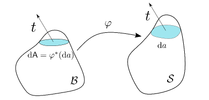
Figure 2: Piola Transform: notice that the length and direction of the force acting an the deformed and reference area is preserved under Piola transform.

The first Piola stress may now be obtained by pulling back the area leg of the Cauchy stress under the deformation map. This partial pull back of the Cauchy stress is termed the Piola transform. This relationship may be formally written as,

$$P =t^{i}\otimes\varphi^{*}(\text{d}a^{i})$$

$$=t^{i}\otimes{\text{d}}\mathsf{A}^{i}$$ (42)

Note that the traction 1-form in both the definitions of Cauchy stress and first Piola stress are the same, i.e. the pull back does nothing to the traction 1-form. In the above discussion, contrary to convention, Cauchy and first Piola stresses are identified as third order tensors, not the usual second order. This ambiguity can be removed if one applies Hodge star on the area leg of these two stresses. In three dimensions, the Hodge star establishes an isomorphism between forms of degree 2 and 1. Applying Hodge star to Cauchy and first Piola stresses leads to,

$$\sigma =t^{i}\otimes({}_{\star}\text{d}a)^{i}$$ (43)

$$P =t^{i}\otimes({}_{\star}\text{d}\mathsf{A})^{i}$$ (44)

Kanso et al. made a distinction between the stress tensors given in (41), (42) and (43), (44). However we do not see a need for it, since both the usual and geometric definitions of stress contain exactly the same information; only the ranks of these tensors are different.

4.1 Traction 1-form via a stored energy function

The Doyle-Ericksen formula is an important result in continuum mechanics [6], which states that the Cauchy stress understood as a 2-tensor and the metric tensor of the deformed configuration are work conjugate pairs. For a stored energy density function $W$, Doyle-Ericksen formula gives us the following relationship,

$$\sigma=2\frac{\partial W}{\partial g}$$ (45)

In writing (45), we have assumed that $W$ depends on the differential of deformation through the right Cauchy-Green deformation tensor, i.e. $W$ is frame-indifferent. From the discussion presented in the previous section, it can be seen that the area leg of the Cauchy stress tensor is determined by the choice of coordinate system for the tangent bundle of the deformed configuration. On the other hand, the area leg of the first Piola stress is determined by both the co-ordinate system for the tangent bundle of the deformed configuration and the deformation map. Clearly, the area leg of a stress tensor does not require a constitutive rule, the only component requiring so is the traction 1-form.

We now claim that for a stored energy function $W$, the traction $1-$form has the following constitutive rule,

$$t^{i}=\frac{1}{J}\frac{\partial W}{\partial e_{i}}$$ (46)

The last equation is in the same spirit as the Doyle-Ericksen formula. To establish the result stated in (46), we first compute the directional derivative of $W$ along $e_{i}$,

$$\frac{\partial W}{\partial e_{i}} =\frac{\partial W}{\partial({\text{d}}\varphi)}\frac{\partial({\text{d}}\varphi)}{\partial e_{i}}$$ (47a)

$$=(t^{j}\otimes{}_{\star}{\text{d}}\mathsf{A}^{k})(e^{i}\otimes e_{j}\otimes\theta^{k})$$ (47b)

$$=\langle{}_{\star}{\text{d}}\mathsf{A}^{J},\theta^{J}\rangle t^{i}$$ (47c)

$$=t^{i}{}_{\star}{\text{d}}\mathsf{V}$$ (47d)

$$=Jt^{i}$$ (47e)

We used chain rule to arrive at the right hand side of (47a). In (47b), the expression for Piola stress (as a two tensor) in terms of $W$ and the directional derivative of ${\text{d}}\varphi$ along $e_{i}$ are used to get the right hand side and performing the required contractions lead to (47c). The claim is finally established by using the definitions of pull back and Hodge star for volume forms. In three dimensions, constitutive relations have to be supplied to the three traction 1-forms each conjugate to vector elements in the frame to close the equations of motion. If the Cauchy stress generated by a stored energy function is known, then the expression for traction 1-form can be computed using the simple relationship $t^{i}=\sigma n^{i}$, where the vector fields $n^{i}$ are chosen to be elements from the frame of the deformed configuration.

5 Hu-Washizu variational principle

We first present the conventional HW variational principle for a finitely deforming elastic body. The HW variational principle takes the deformation gradient, first Piola stress and deformation map as input arguments. The referential version of HW functional for a non-linear elastic solid reads,

$$I_{HW}=\int_{\mathcal{B}}[W(C)-P:(F-{\text{d}}\varphi)]{\text{d}}V-\int_{\partial\mathcal{B}}\langle t,\varphi\rangle{\text{d}}A$$ (48)

In the above equation $t=PN$, is the traction defined on the surface $\partial\mathcal{B}$. The integration in the above equation is withrespect to the volume and the area forms of the reference configuration. In (48), deformation gradient is assumed to be independent, this tensor field is denoted by $F$, while the deformation gradient computed from deformation is denoted by ${\text{d}}\varphi$. Another important point to notice is that the the second term in the above equation is bilinear in Piola stress and deformation gradient. The variation of the HW functional with respect to deformation, deformation gradient and first Piola stress leads to the equilibrium equation, constitutive rule and compatibility of deformation gradient. HW variational principle have been previously exploited to formulate numerical solution procedure to solve non-linear problems in elasticity see[1, 22, 21].

5.1 Hu-Washizu variational principle using geometric definitions of stress and deformation

From now on we will use the definitions of Cauchy and Piola stresses as given in (41) and (42) respectively. We now rewrite the HW variational principle such that it takes deformation 1-forms, traction 1-forms and deformation map as inputs. We also assume that compatible frame fields for the reference and deformed configurations are given. The HW functional may be written as,

$$I(\theta^{i},t^{i},\varphi)=\int_{\mathcal{B}}W(\theta^{i}){\text{d}}V-(t^{i}\otimes{\text{d}}\mathsf{A}^{i})\dot{\wedge}(e_{i}\otimes(\theta^{i}-\text{d}\varphi^{i}))-\int_{\partial\mathcal{B}}\langle t^{\sharp},\varphi\rangle{\text{d}}\mathsf{A}$$ (49)

Note that we did not write the volume form in the second term on the RHS of (49), since the outcome of $\dot{\wedge}$ is a 3-form which can be integrated over the reference configuration to produce work done by the traction 1-forms on the frame fields. In (49), $\dot{\wedge}$ denotes a bilinear map. For $\alpha\in T^{*}\mathcal{S}$, $v\in T\mathcal{S}$ and $a,b\in\Lambda(\mathcal{B})$ the action of this map is given by $(\alpha\otimes a)\dot{\wedge}(v\otimes b)=\alpha(v)a\wedge b$. Note that the definition of $\dot{\wedge}$ given here is a little different from the one in Kanso et al.; specifically, we do not use the metric tensor. From the definition of $\dot{\wedge}$, it can be seen that the work done by stress on deformation is metric independent. This property of our current variational formulation brings the continuum mechanical definition of stress a step closer to the definition of force as defined in classical mechanics. Another important point here is that the second term on the RHS in (49) is equivalent to the second term in (48); however now the relationship between the different arguments is multi-linear.

Remark 1: In writing (49), we have presumed that the geometry of the body is Euclidean and it is frozen during the deformation process. We believe that this assumption can be relaxed by permitting non-integrability in the connections and deformation 1-forms (i.e. by incorporating source terms in the structure equations).

Remark 2: For a frame to represent Euclidean geometry, it is not required that the connection 1-forms be identically zero. It only requires zero source term in Cartan’s structure equations. Any set of (unit) tangent vectors to a curvilinear co-ordinate system will have non-zero connection 1-forms, even as it acts as a frame in the Euclidean space.

We now proceed to obtain the Euler-Lagrange equations or the condition for critical points of the functional $I$. We use the Gateaux derivative for this purpose. Let $\epsilon$ denote a small parameter and $\hat{(.)}$ an increment in quantity with which we are differentiating the functional $I$. We first calculate the variation of $I$ with respect to traction 1-forms; $t^{i}\mapsto t^{i}+\epsilon\hat{t}^{i}$, where $\hat{t}^{i}$ are assumed to be from the tangent space of $T^{*}\mathcal{S}$.

$$I(\epsilon)=\int_{\mathcal{B}}W(\theta^{i})-((t^{i}+\epsilon\hat{t}^{i})\otimes{\text{d}}\mathsf{A}^{i})\dot{\wedge}(e_{j}\otimes(\theta^{j}-\text{d}\varphi^{j}))-\int_{\partial\mathcal{B}}\langle t^{\sharp},\varphi\rangle{\text{d}}\mathsf{A}$$ (50)

Using the definition of $\dot{\wedge}$ and Gateaux derivative, we get a vector valued 3-form for each $i$. These three 3-forms have to be equated to zero to get the condition for critical points in the direction of traction 1-forms. These conditions can be formally written as,

$$\begin{bmatrix}({\text{d}}\mathsf{A}^{1}\wedge(\theta^{1}-{\text{d}}\varphi^{1}))&-({\text{d}}\mathsf{A}^{1}\wedge{\text{d}}\varphi^{2})&-({\text{d}}\mathsf{A}^{1}\wedge{\text{d}}\varphi^{2})\\ -({\text{d}}\mathsf{A}^{2}\wedge{\text{d}}\varphi^{1})&({\text{d}}\mathsf{A}^{2}\wedge(\theta^{2}-{\text{d}}\varphi^{2}))&-({\text{d}}\mathsf{A}^{2}\wedge{\text{d}}\varphi^{2})\\ -({\text{d}}\mathsf{A}^{3}\wedge{\text{d}}\varphi^{1})&-({\text{d}}\mathsf{A}^{3}\wedge{\text{d}}\varphi^{2})&({\text{d}}\mathsf{A}^{3}\wedge(\theta^{3}-{\text{d}}\varphi^{3}))\end{bmatrix}\otimes\begin{bmatrix}e_{1}\\ e_{2}\\ e_{3}\end{bmatrix}=\begin{bmatrix}0\\ 0\\ 0\end{bmatrix}$$ (51)

Since $e_{i}$ are elements form the frame, we have $g(e_{i},e_{i})=1$. The above equation can be true only when the coefficient matrix on the LHS is zero, which leads to,

$$({\text{d}}\mathsf{A}^{1}\wedge(\theta^{1}-{\text{d}}\varphi^{1}))=0;\quad({\text{d}}\mathsf{A}^{1}\wedge{\text{d}}\varphi^{2})=0;\quad({\text{d}}\mathsf{A}^{1}\wedge{\text{d}}\varphi^{2})=0$$ (52a)

$$({\text{d}}\mathsf{A}^{2}\wedge{\text{d}}\varphi^{1})=0;\quad({\text{d}}\mathsf{A}^{2}\wedge(\theta^{2}-{\text{d}}\varphi^{2}))=0;\quad({\text{d}}\mathsf{A}^{2}\wedge{\text{d}}\varphi^{2})=0$$ (52b)

$$({\text{d}}\mathsf{A}^{3}\wedge{\text{d}}\varphi^{1})=0;\quad({\text{d}}\mathsf{A}^{3}\wedge{\text{d}}\varphi^{2})=0;\quad({\text{d}}\mathsf{A}^{3}\wedge(\theta^{3}-{\text{d}}\varphi^{3}))=0$$ (52c)

The above equations can be recast in a matrix form as,

$$\begin{bmatrix}\theta^{1}-{\text{d}}\varphi^{1}&{\text{d}}\varphi^{2}&{\text{d}}\varphi^{3}\\ \theta^{1}&\theta^{2}-{\text{d}}\varphi^{2}&{\text{d}}\varphi^{3}\\ \theta^{1}&{\text{d}}\theta^{2}&{\text{d}}\theta^{3}-\varphi^{3}\end{bmatrix}\wedge\begin{bmatrix}\theta^{2}\wedge\theta^{3}\\ \theta^{3}\wedge\theta^{1}\\ \theta^{1}\wedge\theta^{2}\\ \end{bmatrix}=\begin{bmatrix}0\\ 0\\ 0\end{bmatrix}$$ (53)

For these equations to hold, the following conditions must be met,

$$\theta^{1}-{\text{d}}\varphi^{1}=0;\quad\theta^{2}-{\text{d}}\varphi^{2}=0;\quad\theta^{3}-{\text{d}}\varphi^{3}=0;\quad$$ (54)

The above condition simply states that there exist three zero forms whose exterior derivatives are the deformation 1-forms; or in other words, deformation 1-forms are exact and $\varphi^{i}$ are the potentials for the corresponding deformation 1-forms.

We now compute the variation of $I$ with respect to deformation 1-forms. Incremental changes in the deformation 1-forms may be written as, $\theta^{i}\mapsto\theta^{i}+\epsilon\hat{\theta}^{i}$, where $\epsilon\hat{\theta}^{i}$ is assumed to be an element from the tangent space of $T^{*}\mathcal{B}$.

$$I(\epsilon)=\int_{\mathcal{B}}W(\theta^{i}+\epsilon\hat{\theta}^{i})-(t^{i}\otimes{\text{d}}\mathsf{A}(\epsilon)^{i})\dot{\wedge}(e_{j}\otimes\theta^{j}(\epsilon))-\int_{\partial\mathcal{B}}\langle t^{\sharp},\varphi\rangle{\text{d}}A$$ (55)

Using the definition of Gateaux derivative, for each $\theta^{i}$ we have,

$$\frac{\partial W}{\partial\theta^{1}} =[t^{1}(e_{1}){}_{\star}(\theta^{2}\wedge\theta^{3})-t^{2}(e_{1}){}_{\star}({\text{d}}\varphi^{1}\wedge\theta^{3})+t^{2}(e_{2}){}_{\star}((\theta^{2}-{\text{d}}\varphi^{2})\wedge\theta^{3})-t^{2}(e_{3}){}_{\star}({\text{d}}\varphi^{3}\wedge\theta^{3})$$

$$-t^{3}(e_{1}){}_{\star}(\theta^{2}\wedge\varphi^{1})+t^{3}(e_{2}){}_{\star}(\theta^{2}\wedge{\text{d}}\varphi^{3})+t^{3}(e_{3}){}_{\star}(\theta^{2}\wedge(\theta^{3}-{\text{d}}\varphi^{3}))]^{\sharp}$$ (56a)

$$\frac{\partial W}{\partial\theta^{2}} =[t^{1}(e_{1}){}_{\star}(\theta^{3}\wedge(\theta^{1}-{\text{d}}\varphi^{1}))-t^{1}(e_{2}){}_{\star}(\theta^{3}\wedge{\text{d}}\varphi^{2})-t^{1}(e_{3}){}_{\star}(\theta^{3}\wedge{\text{d}}\varphi^{3})-t^{2}(e_{2}){}_{\star}((\theta^{3}\wedge{\text{d}}\theta^{1})$$

$$-t^{3}(e_{1}){}_{\star}({\text{d}}\varphi^{1}\wedge\theta^{1})-t^{3}(e_{2}){}_{\star}(\theta^{2}\wedge\theta^{1})+t^{3}(e_{3}){}_{\star}((\theta^{3}-{\text{d}}\varphi^{3})\wedge\theta^{1})]^{\sharp}$$ (56b)

$$\frac{\partial W}{\partial\theta^{3}} =[t^{1}(e_{1}){}_{\star}((\theta^{1}-{\text{d}}\varphi^{1})\wedge\theta^{2})-t^{1}(e_{2}){}_{\star}(\varphi^{2}\wedge{\text{d}}\theta^{2})-t^{1}(e_{3}){}_{\star}(\varphi^{3}\wedge{\text{d}}\theta^{2})-t^{2}(e_{1}){}_{\star}({\text{d}}\theta^{1}\wedge{\text{d}}\varphi^{1})$$

$$-t^{2}(e_{2}){}_{\star}(\theta^{1}-(\theta^{2}-\varphi^{2}))+t^{2}(e_{3}){}_{\star}(\theta^{1}\wedge{\text{d}}\varphi^{3})+t^{3}(e_{3}){}_{\star}(\theta^{1}\wedge\theta^{2})]^{\sharp}$$ (56c)

If we now take into account the compatibility equations previously established in (54), the last equations reduce to,

$$\frac{\partial W}{\partial\theta^{1}} =[t^{1}(e_{1}){}_{\star}(\theta^{2}\wedge\theta^{3})+t^{2}(e_{1}){}_{\star}(\theta^{3}\wedge\theta^{1})+t^{3}(e_{1}){}_{\star}(\theta^{2}\wedge\theta^{1})]^{\sharp}$$ (57a)

$$\frac{\partial W}{\partial\theta^{2}} =[t^{1}(e_{2}){}_{\star}(\theta^{2}\wedge\theta^{3})+t^{2}(e_{2}){}_{\star}((\theta^{3}\wedge\theta^{1})+t^{3}(e_{2}){}_{\star}(\theta^{1}\wedge\theta^{2})]^{\sharp}$$ (57b)

$$\frac{\partial W}{\partial\theta^{3}} =[t^{1}(e_{3}){}_{\star}(\theta^{2}\wedge{\text{d}}\theta^{3})+t^{2}(e_{3}){}_{\star}(\theta^{3}\wedge{\text{d}}\theta^{1})+t^{3}(e_{3}){}_{\star}(\theta^{1}\wedge\theta^{2})]^{\sharp}$$ (57c)

From these equations, it is seen that a 2-form accompanies the components of traction 1-forms; this is indeed true since we use a Piola transform to write the constitutive rule in the reference configuration. From a comparison of (56), where Cartan’s structure equations for kinematic closure have not been enforced, and (57), we note that the expressions for traction in the former have additional terms. These additional terms may be related to incompatibilities created by the emergence of defects (such as dislocations) as the deformation evolves. In other words, without an explicit imposition of the kinematic closure conditions on the flow, the deformed body may never be realized as a subset of the Euclidean space.

Finally, we compute the variation of $I$ with respect to deformation; $\varphi^{i}\mapsto\varphi^{i}+\epsilon\hat{\varphi}^{i}$, where $\hat{\varphi}$ belongs to $T\mathcal{B}$. Using the definition of the superimposed incremental deformation in $I$ and upon computing the Gateaux derivative, we have the following equation,

$$\int_{\mathcal{B}}(t^{i}\otimes{\text{d}}\mathsf{A}^{i})\dot{\wedge}(e_{j}\otimes{\text{d}}\hat{\varphi}^{i})=0$$ (58)

To complete the variation, we need to shift the differential from $\hat{\varphi}$. We first calculate the following,

$${\text{d}}(\varphi^{k}t^{j}(e_{k}){\text{d}}\mathsf{A}^{j})={\text{d}}\varphi^{k}\wedge t^{j}(e_{k}){\text{d}}\mathsf{A}^{j}+\varphi^{k}{\text{d}}(t^{j}(e_{k}))\wedge{\text{d}}\mathsf{A}^{j}+\varphi^{k}t^{j}(e_{k}){\text{d}}^{2}\mathsf{A}^{j}$$ (59)

This equation invites a few comments. The first is that we are calculating the exterior derivative of a 2-form, with $\varphi^{k}t^{j}(e_{k})$ being a scalar. Using the product rule of differentiation, we have expanded the right hand side of (59). The second term in (59) should be evaluated using the connection 1-forms since it involves the exterior derivative of a vector. This terms is relevant when one works with a non-trivial connection for the manifold, examples being a body with dislocations and a Kirchhoff shell. If we invoke compatibility of deformation, we have ${\text{d}}^{2}A=0$, which leaves (59) in the following form,

$${\text{d}}(\varphi^{k}t^{j}(e_{k}){\text{d}}\mathsf{A}^{j})={\text{d}}\varphi^{k}\wedge t^{j}(e_{k}){\text{d}}\mathsf{A}^{j}+\varphi^{k}{\text{d}}(t^{j}(e_{k}))\wedge{\text{d}}\mathsf{A}^{j}$$ (60)

An expression similar to (60) was utilized by Kanso et al. [13] to define mechanical equilibrium. The expression for exterior derivative defined in (60) involves the connection 1-forms of the manifold, which is similar to the covariant exterior derivatives used in gauge theories in physics. Using (59) in (58) leads to,

$$\int_{\mathcal{B}}{\text{d}}(\hat{\varphi}^{k}t^{j}(e_{k}){\text{d}}\mathsf{A}^{j})-\hat{\varphi}^{k}{\text{d}}(t^{j}(e_{k}))\wedge{\text{d}}\mathsf{A}^{j}=0$$ (61)

The first term in the above equation can be converted to a boundary term via Stokes’ theorem leading to,

$$\int_{\partial\mathcal{B}}\hat{\varphi}^{k}t^{j}(e_{k}){\text{d}}\mathsf{A}^{j}-\int_{\mathcal{B}}\hat{\varphi}^{k}{\text{d}}(t^{j}(e_{k}))\wedge{\text{d}}\mathsf{A}^{j}=0$$ (62)

Using the arbitrariness of $\hat{\varphi}^{k}$, we conclude that,

$${\text{d}}(t^{j}(e_{k}))\wedge{\text{d}}\mathsf{A}^{j}=0$$ (63)

This is the condition for the critical point of the energy functional in the direction of deformation, which is nothing but the balance of forces. Note that the connection 1-forms of the deformed configuration appear through the exterior derivative of the deformed configuration’s frame field.

5.2 Stress a Lagrange multiplier

For a hyper-elastic solid, stress is derived from a stored energy function which may be written as a function of the deformation gradient. This assumption permits us to write the equations of equilibrium as the Euler-Lagrange equation of the stored energy functional. In a certain sense, the stress generated in a hyper-elastic solid should satisfy certain integrability condition (i.e. the existence of the stored energy function). Moreover, if we assume the stored energy function to be translation and rotation invariant, it implies equilibrium of forces and moments. Thus for the hyper-elastic solid, balances of force and moment are consequences of translation and rotation invariance; stress is only a secondary variable introduced for writing the equations of equilibrium in a convenient way.

When formulated as a mixed problem, the stress tensor has a completely different role. Our HW functional has deformation, deformation 1-forms and stress 2-forms as inputs. For a stored energy function, viewed as a function of deformation 1-forms, translation and rotation invariance cannot be discussed directly, since nothing about the geometry of the co-tangent bundle from which the deformation 1-forms were pulled back is known. In other words, there is nothing in the stored energy function that requires the base space of the deformed configurations co-tangent bundle to be Euclidean. The second term in (49) is introduced to imposes this constraint. Observe that, in (49), the second term is multilinear in the input arguments, vis-á-vis, stress 2-forms, differential of deformation and deformation 1-forms. The stress $2-$form can now be thought as a Lagrange multiplier introduced to impose the equality between differential of deformation and deformation 1-forms. Alternatively, the equality between the differential of deformation and deformation 1-forms implies that the deformed configuration is Eulclidean.

6 Conclusion

We have formulated the HW variational principle using differential forms. The main tenets of this reformulation are Cartan’s method of moving frames and the interpretation of stress as a co-vector valued 2-form. The Euler-Lagrange equations clearly explicate how additional stresses could be generated when the kinematic closure or compatibility conditions are not explicitly imposed. These stresses are the result of incompatibilities that develop and co-evolve with the deformation and may render the deformed solid body non-Euclidean. In this sense, the present variational approach may be used not only with models that aim at restricting the deformed body as a subset of the Euclidean space, but also with those where the evolution of incompatibilities, e.g. defects, is of importance.

Our novel approach to the HW variational principle also has consequences in the numerical solution of the equations of nonlinear elasticity. The discretization schemes based on finite element exterior calculus may now be seamlessly used to approximate the differential forms appearing in the HW functional. Such an approximation has the advantage of respecting the algebraic and geometric structures defined by these differential forms even after discretization. Work is currently under way to study such approximations.

The kinematic framework developed to describe deformation has a specific advantage in modelling the motion of shells. In the case of shells, the differential of the position vector is non-trivial since the tangent spaces at different material points are not the same. When tied with Cartan’s moving frames, the kinematics of the shell surface can be completely reformulated in terms of differential forms. The stress resultants may then be understood as bundle valued differential forms. These kinetic and kinematic ideas may then be stitched together using the new HW principle, to arrive at a shell theory that is transparent in its geometric assumptions.

References

- [1] A. Angoshtari, M. F. Shojaei, and A. Yavari. Compatible-strain mixed finite element methods for 2d compressible nonlinear elasticity. Computer Methods in Applied Mechanics and Engineering, 313:596–631, 2017.
- [2] D. Arnold, R. Falk, and R. Winther. Finite element exterior calculus: from hodge theory to numerical stability. Bulletin of the American mathematical society, 47(2):281–354, 2010.
- [3] D. N. Arnold, R. S. Falk, and R. Winther. Finite element exterior calculus, homological techniques, and applications. Acta numerica, 15:1–155, 2006.
- [4] J. M. Ball and G. Knowles. A numerical method for detecting singular minimizers. Numerische Mathematik, 51(2):181–197, 1987.
- [5] A. Bossavit. Whitney forms: A class of finite elements for three-dimensional computations in electromagnetism. IEE Proceedings A (Physical Science, Measurement and Instrumentation, Management and Education, Reviews), 135(8):493–500, 1988.
- [6] T. Doyle and J. L. Ericksen. Nonlinear elasticity. In Advances in applied mechanics, volume 4, pages 53–115. Elsevier, 1956.
- [7] A. C. Eringen. Microcontinuum field theories: I. Foundations and solids. Springer Science & Business Media, 2012.
- [8] H. Flanders. Differential Forms with Applications to the Physical Sciences by Harley Flanders. Elsevier, 1963.
- [9] H. Guggenheimer. Differential Geometry. McGraw-Hill series in higher mathematics. McGraw-Hill, 1963.
- [10] F. W. Hehl and Y. N. Obukhov. Foundations of classical electrodynamics: Charge, flux, and metric, volume 33. Springer Science & Business Media, 2012.
- [11] R. Hiptmair. Canonical construction of finite elements. Mathematics of computation, 68(228):1325–1346, 1999.
- [12] A. N. Hirani. Discrete exterior calculus. PhD thesis, California Institute of Technology, 2003.
- [13] E. Kanso, M. Arroyo, Y. Tong, A. Yavari, J. G. Marsden, and M. Desbrun. On the geometric character of stress in continuum mechanics. Zeitschrift für angewandte Mathematik und Physik, 58(5):843–856, 2007.
- [14] J. E. Marsden and T. J. Hughes. Mathematical foundations of elasticity. Courier Corporation, 1994.
- [15] J. E. Marsden and T. S. Ratiu. Introduction to mechanics and symmetry: a basic exposition of classical mechanical systems, volume 17. Springer Science & Business Media, 2013.
- [16] J.-C. Nédélec. Mixed finite elements in . Numerische Mathematik, 35(3):315–341, 1980.
- [17] J.-C. Nédélec. A new family of mixed finite elements in . Numerische Mathematik, 50(1):57–81, 1986.
- [18] R. W. Ogden. Non-linear elastic deformations. Courier Corporation, 1997.
- [19] P.-A. Raviart and J.-M. Thomas. A mixed finite element method for 2-nd order elliptic problems. In Mathematical aspects of finite element methods, pages 292–315. Springer, 1977.
- [20] S. Sadik and A. Yavari. On the origins of the idea of the multiplicative decomposition of the deformation gradient. Math. Mech. Solids, 22(4):771–772, 2017.
- [21] M. F. Shojaei and A. Yavari. Compatible-strain mixed finite element methods for incompressible nonlinear elasticity. Journal of Computational Physics, 361:247–279, 2018.
- [22] M. F. Shojaei and A. Yavari. Compatible-strain mixed finite element methods for 3d compressible and incompressible nonlinear elasticity. Computer Methods in Applied Mechanics and Engineering, 357:112610, 2019.
- [23] J. C. Simo and D. D. Fox. On a stress resultant geometrically exact shell model. i: Formulation and optimal parametrization. Computer Methods in Applied Mechanics and Engineering, 72(3):267–304, 1989.
- [24] L. Tu. An Introduction to Manifolds. Universitext. Springer New York, 2010.
- [25] A. Yavari. On geometric discretization of elasticity. Journal of Mathematical Physics, 49(2):022901, 2008.