On some 4-by-4 matrices
with bi-elliptical numerical ranges.

Abstract

A complete description of 4-by-4 matrices $\begin{bmatrix}\alpha I&C\\ D&\beta I\end{bmatrix}$, with scalar 2-by-2 diagonal blocks, for which the numerical range is the convex hull of two non-concentric ellipses is given. This result is obtained by reduction to the leading special case in which $C-D^{*}$ also is a scalar multiple of the identity. In particular cases when in addition $\alpha-\beta$ is real or pure imaginary, the results take an especially simple form. An application to reciprocal matrices is provided.

1 Introduction

The numerical range of a matrix $A\in\mathbb{C}^{n\times n}$ is defined as

$$W(A)=\{\langle Ax,x\rangle\colon x\in\mathbb{C}^{n},\ \left\|x\right\|=1\}.$$

We are using the standard notation $\langle.,.\rangle$ for the inner product on the $n$-dimensional space $\mathbb{C}^{n}$ and $\left\|.\right\|$ for the norm associated with it: $\left\|x\right\|^{2}=\langle x,x\rangle$.

It is well known that $W(A)$ is a convex compact subset of $\mathbb{C}$ containing the spectrum $\sigma(A)$ of $A$, and thus its convex hull $\operatorname{conv}\sigma(A)$. For normal matrices $A$, the equality $W(A)=\operatorname{conv}\sigma(A)$ holds. On the other hand, for non-normal $A\in\mathbb{C}^{2\times 2}$ the numerical range is an elliptical disk, with the foci at the eigenvalues. These and other by now classical properties of $W(A)$ can be found, e.g., in [7, Chapter 1] or more recent [3, Chapter 6].

The shape of $W(A)$ for $A\in\mathbb{C}^{3\times 3}$ is also known, see [9] (or its translation [10] into English) for the classification and [8] for the pertinent tests. However, for $n\geq 4$ many questions remain open. In particular, it is of interest when the boundary $\partial W(A)$ of the numerical range contains an elliptical arc [5].

A useful tool in studying properties of $W(A)$ is the so called Numerical range (NR) generating curve $C(A)$, also introduced in [9] — the Kippenhahn curve in the terminology of [3, Chapter 13], where a very lucid and detailed description of $C(A)$ is given. This curve is defined uniquely by having exactly $n$ tangent lines in each direction $e^{i\theta}$, intercepting the family of orthogonal lines at the eigenvalues $\lambda_{j}(\theta)$ of $\operatorname{Im}(e^{-i\theta}A)$. As it happens, $W(A)=\operatorname{conv}C(A)$, and so $\partial W(A)$ consists of some arcs of $C(A)$ possibly connected by line segments.

We will denote the characteristic polynomial of $\operatorname{Im}(e^{-i\theta}A)$ by $P_{A}(\lambda,\theta)$ and call it the NR generating polynomial of $A$. From the description of $C(A)$ it follows in particular that it contains an ellipse if and only if $P_{A}(\lambda,\theta)$ is divisible by a polynomial quadratic in $\lambda$. More specifically (as can be established by direct computations similar to those carried out say in [2]), an ellipse centered at $p+iq$ ($p,q\in\mathbb{R}$) corresponds to a factor of the form

$$\quad(\lambda+p\sin\theta-q\cos\theta)^{2}+x\cos 2\theta+y\sin 2\theta-z$$ (1.1)

with some $x,y,z\in\mathbb{R}$ satisfying $z\geq\sqrt{x^{2}+y^{2}}$. Note that if $z=\sqrt{x^{2}+y^{2}}$, then the quadratic (1.1) factors further into two linear functions in $\lambda$, and the ellipse in question degenerates into the doubleton of its foci.

If $n=4$ and $P_{A}(\lambda,\theta)$ is divisible by (1.1), then the quotient is of the same type. Consequently, for $A\in\mathbb{C}^{4\times 4}$ the boundary of $W(A)$ contains an elliptical arc if and only if $C(A)$ consists of two ellipses, one of which is possibly degenerate. So, $\partial W(A)$ contains an elliptical arc if and only if $W(A)$ is an elliptical disk, the convex hull of two ellipses, or the convex hull of an ellipse and one or two points (the latter being an option only if $A$ is unitarily reducible). The respective criteria were established in [4]. However, these criteria are not stated in terms of $A$ directly and therefore not easy to verify. More can be done if $A$ enjoys some additional structure.

This paper is devoted to 4-by-4 matrices of the form

$$\quad A=\begin{bmatrix}\alpha I&C\\ D&\beta I\end{bmatrix}.$$ (1.2)

In [6, Section 4], we have provided necessary and sufficient conditions for such matrices to have $W(A)$ in the shape of an elliptical disk or the convex hull of two concentric ellipses. Here we treat the remaining case, when $W(A)$ is the convex hull of two ellipses with distinct centers. For convenience of reference, this shape is called bi-elliptical in what follows.

The special case of matrices (1.2) with $C-D^{*}$ being a scalar multiple of the identity is considered in Section 3, after some preliminary technicalities disposed of in Section 2. Under additional restrictions on $\alpha-\beta$, this result is further simplified in Section 4 which also contains several numerical examples. As it happens, the general case can be reduced to the one tackled in Section 3; this reduction is carried over in Section 5. The final Section 6 contains an application to so called reciprocal matrices.

2 Preliminary results

Passing from $A$ to $A-\frac{\alpha+\beta}{2}I$, we may (and will, in what follows) without loss of generality suppose that in (1.2) $\beta=-\alpha$. As in [6], we will also use the notation

$$\quad H=C^{*}C+DD^{*},\quad Z=DC.$$ (2.1)

Lemma 1.

Let $A$ be given by (1.2), with $\beta=-\alpha$. Then:

(i) The eigenvalues of $A$ are $\pm\sigma_{1},\ \pm\sigma_{2}$, where $\sigma_{j}=\sqrt{z_{j}+\alpha^{2}}$ and $z_{1},z_{2}$ are the eigenvalues of $Z$;

(ii) The eigenvalues of $\operatorname{Im}(e^{-i\theta}A)$ are $\pm\lambda_{j}(\theta)$, where

$$\lambda_{j}(\theta)=\sqrt{(\operatorname{Im}(e^{-i\theta}\alpha))^{2}+\mu_{j}(\theta)/4}\quad(j=1,2),$$

and $\mu_{j}(\theta)$ are the eigenvalues of

$$\quad\left(e^{i\theta}C^{*}-e^{-i\theta}D\right)\left(e^{-i\theta}C-e^{i\theta}D^{*}\right)=H-2\operatorname{Re}(e^{-2i\theta}Z);$$ (2.2)

(iii) The NR generating polynomial $P_{A}$ of $A$ is $\lambda^{4}-\Xi_{1}(\theta)\lambda^{2}+\Xi_{2}(\theta)$, where

$$\Xi_{1}(\theta)=\frac{1}{4}\operatorname{Tr}H+|\alpha|^{2}-\left(\frac{1}{2}\operatorname{Re}\operatorname{Tr}Z+\operatorname{Re}\alpha^{2}\right)\cos 2\theta\\ -\left(\frac{1}{2}\operatorname{Im}\operatorname{Tr}Z+\operatorname{Im}\alpha^{2}\right)\sin 2\theta,$$ (2.3)

$$16\Xi_{2}(\theta)=6|\alpha|^{4}+2|\alpha|^{2}\operatorname{Tr}H+2\operatorname{Re}(\overline{\alpha^{2}}\operatorname{Tr}Z)+\frac{1}{2}\operatorname{Tr}(H)^{2}-\frac{1}{2}\operatorname{Tr}(H^{2})+|\operatorname{Tr}(Z)|^{2}\\ -\operatorname{Tr}(ZZ^{*})-\operatorname{Re}\zeta_{1}\cos 2\theta-\operatorname{Im}\zeta_{1}\sin 2\theta+\operatorname{Re}\zeta_{2}\cos 4\theta+\operatorname{Im}\zeta_{2}\sin 4\theta,$$ (2.4)

with $\zeta_{1},\zeta_{2}$ given by

$$\zeta_{1} =8|\alpha|^{2}\alpha^{2}+2\alpha^{2}\operatorname{Tr}H+4|\alpha|^{2}\operatorname{Tr}Z+2\operatorname{Tr}Z\operatorname{Tr}H-2\operatorname{Tr}ZH,$$

$$\zeta_{2} =2\det Z+2\alpha^{2}\operatorname{Tr}Z+2\alpha^{4}.$$

Proof.

For (i) and (ii), the result follows by using Schur complement formula when computing the respective characteristic polynomials; the pertinent computation for (ii) is actually contained in the proof of [6, Lemma 2.1]. Expanding $P_{A}(\lambda,\theta)=(\lambda^{2}-\lambda_{1}^{2}(\theta))(\lambda^{2}-\lambda_{2}^{2}(\theta))$, we derive (iii) from (ii). ∎

Observe that $P_{A}$ is an even function of $\lambda$. This agrees with the result of [6] for matrices (1.2) with arbitrary block sizes, implying that $C(A)$ is symmetric with respect to the origin. From here we immediately obtain

Proposition 1.

Suppose $A\in\mathbb{C}^{4\times 4}$ of the form (1.2) is such that $C(A)$ consists of two non-concentric ellipses. Then, for an appropriate choice of signs of $\sigma_{j}$, $\partial W(A)$ contains a pair of parallel line segments coinciding in length and direction with $\sigma_{1}+\sigma_{2}$.

Proof.

Let $C(A)$ consist of the ellipses $E_{1},E_{2}$. Due to the central symmetry of $C(A)$, either both $E_{1},E_{2}$ also are symmetric with respect to the origin, or $E_{1}(:=E)=-E_{2}\neq-E$. The former case is excluded, because otherwise $E_{1},E_{2}$ would be concentric. Furthermore, the foci of $\pm E$ are the eigenvalues of $A$, and so (relabeling $z_{1},z_{2}$ if needed, and choosing the square roots signs appropriately) we may suppose that $\sigma_{1},\sigma_{2}$ are the foci of $E$.

Consider now the composition $\mathcal{S}$ of two symmetries, one with respect to the origin and the other with respect to the center of $E$. By its construction, $\mathcal{S}$ is a shift and, since $\mathcal{S}(-(\sigma_{1}+\sigma_{2})/2)=(\sigma_{1}+\sigma_{2})/2$, it is the shift by $\sigma_{1}+\sigma_{2}$. So,

$$E={\mathcal{S}}(-E)=-E+(\sigma_{1}+\sigma_{2}).$$

The flat portions on the boundary of $W(A)$ are therefore the common tangents of $E$ and $-E$, and the endpoints of each differ by $\sigma_{1}+\sigma_{2}$. ∎

3 Leading special case

Let

$$\quad A=\begin{bmatrix}\alpha I&B^{*}+I\\ B-I&-\alpha I\end{bmatrix}.$$ (3.1)

This is a particular case of (1.2) in which $C=B^{*}+I$ and $D=B-I$. Respectively, (2.1) takes the form

$$\quad H=2(BB^{*}+I),\quad Z=BB^{*}-I+2i\operatorname{Im}B.$$ (3.2)

Let us denote the eigenvalues of $\operatorname{Im}B$ by $\beta_{1},\beta_{2}$ while keeping the notation $\pm\sigma_{j}$ for the eigenvalues of $A$. Let us also write $\alpha$ as $u+iv$ ($u,v\in\mathbb{R}$).

Theorem 2.

For $A$ as in (3.1), $W(A)$ is bi-elliptical if and only if $B$ is not normal and

$$\quad(1+v^{2})(\sigma_{1}+\sigma_{2})^{2}=(\beta_{1}-\beta_{2})^{2}.$$ (3.3)

Both in the proof of Theorem 2 and its further application, putting block $B$ in an upper triangular form

$$\quad B=\begin{bmatrix}b_{1}&b\\ 0&b_{2}\end{bmatrix}$$ (3.4)

and rewording conditions in terms of its entries proves to be useful. This can be done by a block diagonal unitary similarity of $A$, preserving its structure (3.1). Moreover, it can be arranged that $b\geq 0$. So, without loss of generality

$$\quad A=\begin{bmatrix}\alpha&0&\overline{b_{1}}+1&0\\ 0&\alpha&b&\overline{b_{2}}+1\\ b_{1}-1&b&-\alpha&0\\ 0&b_{2}-1&0&-\alpha\end{bmatrix}.$$ (3.5)

Let us also denote $\operatorname{Re}b_{j}=\xi_{j},\ \operatorname{Im}b_{j}=\eta_{j},\ j=1,2$.

Plugging in the values of $\sigma_{j}$ from Lemma 1, condition (3.3) can be rewritten as

$$\quad\operatorname{Tr}Z+2\alpha^{2}+2\sqrt{\det Z+\alpha^{2}\operatorname{Tr}Z+\alpha^{4}}=4p^{2},$$ (3.6)

where

$$\quad\sqrt{\frac{(\eta_{1}-\eta_{2})^{2}+b^{2}}{1+v^{2}}}:=2p.$$ (3.7)

Rewriting (3.6) as

$$2\sqrt{\det Z+\alpha^{2}\operatorname{Tr}Z+\alpha^{4}}=4p^{2}-\operatorname{Tr}Z-2\alpha^{2}$$

and taking the square, we find that (3.3) is equivalent to $T=0$, where

$$\quad T:=16p^{4}-(8\operatorname{Tr}Z+16\alpha^{2})p^{2}+(\operatorname{Tr}Z)^{2}-4\det Z.$$ (3.8)

This condition is in its turn equivalent to both $\operatorname{Re}T$ and $\operatorname{Im}T$ being equal to zero. For future use observe therefore that

$$\operatorname{Re}T= \left(4p^{2}-(b^{2}+\left|b_{1}\right|^{2}+\left|b_{2}\right|^{2})\right)^{2}-16u^{2}p^{2}-4\left|b_{1}\right|^{2}\left|b_{2}\right|^{2},$$ (3.9)

$$\operatorname{Im}T= 16v\left(v(\eta_{1}+\eta_{2})-2u\right)p^{2}+4(\xi_{1}^{2}-\xi_{2}^{2})(\eta_{1}-\eta_{2}).$$ (3.10)

Proof of Theorem 2. Necessity. If $B$ is normal then it follows from (3.2) that so is $Z$. Moreover, $Z$ and $H$ commute. This situation falls under the setting of [6, Theorem 4.1], according to which $W(A)$ is the convex hull of two ellipses, but these ellipses are concentric. So, $B$ is not normal.

After yet another unitary (this time, permutational) similarity, the matrix (3.5) becomes

$$A_{0}=\begin{bmatrix}\alpha&\overline{b_{1}}+1&0&0\\ b_{1}-1&-\alpha&b&0\\ 0&b&\alpha&\overline{b_{2}}+1\\ 0&0&b_{2}-1&-\alpha\end{bmatrix}.$$

This matrix is tridiagonal. Moreover, $b\neq 0$ since $B$ is not normal. In terminology of [1] it implies that $A_{0}$ is proper (meaning that entries in the positions $(j-1,j)$ and $(j,j-1)$ cannot simultaneously equal zero). Invoking [1, Theorem 10], we conclude that the only flat portions of $\partial W(A)$ are horizontal. Their $y$-coordinates are determined by the eigenvalues of $\operatorname{Im}A_{0}$, which is the direct sum of two copies of $\begin{bmatrix}v&-i\\ i&-v\end{bmatrix}$, and therefore equal $\pm\sqrt{1+v^{2}}$. The lengths of these portions are equal to the spread of the compression $H_{0}$ of $\operatorname{Re}A_{0}$ onto the (2-dimensional) subspace generated by the eigenvectors of $\operatorname{Im}A_{0}$ corresponding to either of its eigenvalues. Denoting $f=\sqrt{1+v^{2}}-v$ and $k=1/\sqrt{1+f^{2}}$, an orthonormal basis in one of these subspaces can be chosen as

$$k[-i,f,0,0]^{T}\text{ and }k[0,0,-i,f]^{T}.$$

The matrix of $H_{0}$ in this basis is

$$\frac{1}{2\sqrt{1+v^{2}}}\begin{bmatrix}u(f^{-1}-f)+2\eta_{1}&-ib\\ ib&u(f^{-1}-f)+2\eta_{2}\end{bmatrix},$$

and the spread of this matrix equals $2p$ defined by (3.7). It remains to observe that $(\beta_{1}-\beta_{2})^{2}=(\eta_{1}-\eta_{2})^{2}+b^{2}$ and to make use of Proposition 1.

Sufficiency. Suppose that (3.3) holds. We will now show that under this condition the NR generating polynomial of $A$ factors as

$$\quad P_{A}(\lambda,\theta)=\left((\lambda+p\sin\theta)^{2}+\Omega(\theta)\right)\left((\lambda-p\sin\theta)^{2}+\Omega(\theta)\right),$$ (3.11)

where $\Omega(\theta)=x\cos 2\theta+y\sin 2\theta-z$ for some appropriate choice of real parameters $x,y,z$.

According to Lemma 1(iii), (3.11) is equivalent to

$$\quad 2\left(p^{2}\sin^{2}\theta-\Omega(\theta)\right)=\Xi_{1}(\theta),\quad\left(p^{2}\sin^{2}\theta+\Omega(\theta)\right)^{2}=\Xi_{2}(\theta),$$ (3.12)

where $\Xi_{1}$ and $\Xi_{2}$ are given by (2.3) and (2.4), respectively. The first equality in (3.12) defines $x,y,z$ uniquely as

$$\quad\begin{cases}x=\frac{1}{4}\operatorname{Re}\operatorname{Tr}Z+\frac{1}{2}\operatorname{Re}(\alpha^{2})-\frac{p^{2}}{2},\\ y=\frac{1}{4}\operatorname{Im}\operatorname{Tr}Z+\frac{1}{2}\operatorname{Im}(\alpha^{2}),\\ z=\frac{1}{8}\operatorname{Tr}H+\frac{|\alpha|^{2}}{2}-\frac{p^{2}}{2},\end{cases}$$ (3.13)

or, in terms of $B$ directly:

$$\quad\begin{cases}x=\frac{1}{4}(b^{2}+|b_{1}|^{2}+|b_{2}|^{2}-2)+\frac{1}{2}\operatorname{Re}(\alpha^{2})-\frac{1}{8}\frac{b^{2}+(\eta_{1}-\eta_{2})^{2}}{1+v^{2}},\\ y=\frac{1}{2}(\eta_{1}+\eta_{2})+\frac{1}{2}\operatorname{Im}(\alpha^{2}),\\ z=\frac{1}{4}(b^{2}+|b_{1}|^{2}+|b_{2}|^{2}+2)+\frac{1}{2}|\alpha|^{2}-\frac{1}{8}\frac{b^{2}+(\eta_{1}-\eta_{2})^{2}}{1+v^{2}}.\end{cases}$$ (3.14)

Incidentally, with this choice of $x,y,z$, the second equality in (3.12) also holds. Here is the pertinent chain of computations. First, form (3.13):

$$4\left[p^{2}\sin^{2}(\theta)+\Omega(\theta)\right] =-\frac{1}{2}\operatorname{Tr}H-2|\alpha|^{2}+4p^{2}$$

$$+\left[\operatorname{Re}\operatorname{Tr}Z+2\operatorname{Re}(\alpha^{2})-4p^{2}\right]\cos 2\theta$$

$$+\left[\operatorname{Im}\operatorname{Tr}Z+2\operatorname{Im}(\alpha^{2})\right]\sin 2\theta$$

Squaring we obtain:

$$16\left[p^{2}\sin^{2}(\theta)+\Omega(\theta)\right]^{2}$$

$$=24p^{4}-4p^{2}\left(\operatorname{Re}(\operatorname{Tr}Z+2\alpha^{2})+\operatorname{Tr}H+4|\alpha|^{2}\right)$$

$$+\frac{1}{2}|\operatorname{Tr}Z+2\alpha^{2}|^{2}+\left(\frac{1}{2}\operatorname{Tr}H+2|\alpha|^{2}\right)^{2}$$

$$-8\operatorname{Re}\left[\left(2p^{2}-\frac{1}{2}\operatorname{Tr}Z-\alpha^{2}\right)\left(2p^{2}-\frac{1}{4}\operatorname{Tr}H-|\alpha|^{2}\right)\right]\cos 2\theta$$

$$-8\operatorname{Im}\left[\left(2p^{2}-\frac{1}{2}\operatorname{Tr}Z-\alpha^{2}\right)\left(2p^{2}-\frac{1}{4}\operatorname{Tr}H-|\alpha|^{2}\right)\right]\sin 2\theta$$

$$+2\operatorname{Re}\left[(2p^{2}-\frac{1}{2}\operatorname{Tr}Z-\alpha^{2})^{2}\right]\cos 4\theta$$

$$+2\operatorname{Im}\left[(2p^{2}-\frac{1}{2}\operatorname{Tr}Z-\alpha^{2})^{2}\right]\sin 4\theta.$$

Plugging in $\Xi_{2}$ from (2.4):

$$32\left[\left(p^{2}\sin^{2}\theta+\Omega(\theta)\right)^{2}-\Xi_{2}(\theta)\right]$$ (3.15)

$$=3\bigg{[}16p^{4}-\frac{8}{3}\left(\operatorname{Re}(\operatorname{Tr}Z+2\alpha^{2})+\operatorname{Tr}H+4|\alpha|^{2}\right)p^{2}$$

$$+\frac{2}{3}\operatorname{Tr}(Z^{*}Z)-\frac{1}{3}|\operatorname{Tr}Z|^{2}+\frac{1}{3}\operatorname{Tr}(H^{2})-\frac{1}{6}\operatorname{Tr}(H)^{2}\bigg{]}$$

$$-4\operatorname{Re}\left[16p^{4}-2(\operatorname{Tr}H+2\operatorname{Tr}Z+4\alpha^{2}+4|\alpha|^{2})p^{2}+\operatorname{Tr}ZH-\frac{1}{2}\operatorname{Tr}Z\operatorname{Tr}H\right]\cos 2\theta$$

$$-2\operatorname{Im}\left[-8(\operatorname{Tr}Z+2\alpha^{2})p^{2}+2\operatorname{Tr}ZH-\operatorname{Tr}Z\operatorname{Tr}H\right]\sin 2\theta$$

$$+\operatorname{Re}\left[16p^{4}-8(\operatorname{Tr}Z+2\alpha^{2})p^{2}+(\operatorname{Tr}Z)^{2}-4\det(Z)\right]\cos 4\theta$$

$$+\operatorname{Im}\left[-8(\operatorname{Tr}Z+2\alpha^{2})p^{2}+(\operatorname{Tr}Z)^{2}-4\det(Z)\right]\sin 4\theta.$$

Rewriting the right hand side of (3.15) in terms of the entries of $B$ we obtain, with the use of (3.9)–(3.10):

$$\left(p^{2}\sin^{2}\theta+\Omega(\theta)\right)^{2}-\Xi_{2}(\theta)$$

$$=\frac{1}{32}\left[3\operatorname{Re}T-4\operatorname{Re}T\cos 2\theta-2\operatorname{Im}T\sin 2\theta+\operatorname{Re}T\cos 4\theta+\operatorname{Im}T\sin 4\theta\right].$$

So, condition (3.3), equivalent to $T=0$, indeed implies the second equality in (3.12).

Finally, from (3.14): $z=x+(1+v^{2})$, and furthermore,

$$z^{2}-x^{2}-y^{2}=(1+v^{2})^{2}+2(1+v^{2})x-y^{2}\\ =\frac{(1+v^{2})(\xi_{1}^{2}+\xi_{2}^{2})}{2}+\frac{(1+2v^{2})b^{2}}{4}+\left[u-\frac{(\eta_{1}+\eta_{2})v}{2}\right]^{2}+\frac{v^{2}(\eta_{1}-\eta_{2})^{2}}{4}>0$$

since $b\neq 0$. Factorization (3.11) therefore generates $C(A)$ consisting of two non-degenerate ellipses. ∎

4 Follow up observations and examples

Suppose that in (3.1) the parameter $\alpha$ is real or pure imaginary. Criterion established in Section 3 can then be recast explicitly in terms of $B$. This is done in two theorems below, stated for $B$ as in (3.4). Note however that the results can be easily reworded without putting $B$ in a triangular form. Indeed, $\{b_{1},b_{2}\}$ is the spectrum of $B$, while $b^{2}=\left\|B\right\|_{F}-\left|b_{1}\right|^{2}-\left|b_{2}\right|^{2}$, with $\left\|.\right\|_{F}$ denoting the Frobenius norm.

Theorem 3.

Let $\alpha(=u)\in\mathbb{R}$. Then the numerical range of matrix (3.5) is bi-elliptical if and only if $b\neq 0$ and either
(i) $\eta_{1}=\eta_{2}$ and $4b^{2}u^{2}=\left(\xi_{1}^{2}-\xi_{2}^{2}\right)^{2}$, or (ii) $u=\xi_{1}=\xi_{2}=0$.

Proof.

Since $v=0$, according to (3.10) $\operatorname{Im}T=0$ if and only if $\eta_{1}=\eta_{2}$ or $\xi_{1}^{2}=\xi_{2}^{2}$. On the other hand, $4p^{2}=(\eta_{1}-\eta_{2})^{2}+b^{2}$ due to (3.7), and so (3.9) takes the form

$$\quad\left((\eta_{1}-\eta_{2})^{2}-(\left|b_{1}\right|^{2}+\left|b_{2}\right|^{2})\right)^{2}-4u^{2}\left((\eta_{1}-\eta_{2})^{2}+b^{2}\right)-4\left|b_{1}\right|^{2}\left|b_{2}\right|^{2}.$$ (4.1)

If $\eta_{1}=\eta_{2}$, then (4.1) vanishing amounts to $\left(\left|b_{1}\right|^{2}-\left|b_{2}\right|^{2}\right)^{2}=4u^{2}b^{2}$, which is exactly case (i). If $\eta_{1}\neq\eta_{2}$, denote the coinciding values of $\xi_{1}^{2}$ and $\xi_{2}^{2}$ by $\xi^{2}$. Expression (4.1) then simplifies to

$$-4\xi^{2}(\eta_{1}-\eta_{2})^{2}-4u^{2}\left((\eta_{1}-\eta_{2})^{2}+b^{2}\right),$$

and so it vanishes if and only if $u=\xi=0$. This is case (ii). ∎

Corollary 1.

Let $A$ be of the form (3.5) with zero main diagonal. Then $W(A)$ is bi-elliptical if and only if $b\neq 0$ and either
(i) $\operatorname{Im}b_{1}=\operatorname{Im}b_{2}$ and $\left|b_{1}\right|=\left|b_{2}\right|$, or (ii) $\operatorname{Re}b_{1}=\operatorname{Re}b_{2}=0$.

Note that in [11, Theorem 3.14] the result of Corollary 1 was established under additional restrictions $b=\sqrt{(1-\left|b_{1}\right|)^{2}(1-\left|b_{2}\right|)^{2}}$, $\left|b_{1}\right|,\left|b_{2}\right|<1$.

According to Corollary 1, for $\alpha=0$ the value of $b$ is irrelevant (as long as it is different from zero, of course). The situation is quite the opposite for non-zero values of $\alpha$.

Corollary 2.

Let $A$ be of the form (3.5) with $\alpha\neq 0$. Then there is at most one value of $b(>0)$ for which $W(A)$ is bi-elliptical.

Proof.

For $\alpha\in\mathbb{R}$ the result follows from Theorem 3, with an explicit expression for $b$. For non-real values of $\alpha$, observe that condition $\operatorname{Re}T=0$ with the use of (3.7) and (3.9) yields a quadratic equation for $b^{2}$ with one non-positive root, and thus a unique positive one. ∎

It is possible to derive the explicit value of $b$ for non-real $\alpha$ as well, but the expression is somewhat cumbersome. We will restrict our attention to another special case, when $\alpha$ is pure imaginary.

Theorem 4.

Let $\alpha$ be pure imaginary: $\alpha=iv\neq 0$. Then the numerical range of matrix (3.5) is bi-elliptical if and only if $b\neq 0$,

$$\quad\left|b_{1}\right|=\left|b_{2}\right|,\text{ and }v^{2}b^{2}=(\eta_{1}-\eta_{2})^{2}.$$ (4.2)

Proof.

Setting $u=0$ in (3.9) and (3.10), we see that conditions $\operatorname{Re}T=0$ and $\operatorname{Im}T=0$ simplify respectively to

$$\quad 4p^{2}-b^{2}=\left(\left|b_{1}\right|\pm\left|b_{2}\right|\right)^{2}$$ (4.3)

and

$$\quad 4v^{2}p^{2}(\eta_{1}+\eta_{2})+(\xi_{1}^{2}-\xi_{2}^{2})(\eta_{1}-\eta_{2})=0.$$ (4.4)

Moreover, due to (3.7) and (4.3):

$$4v^{2}p^{2}=(\eta_{1}-\eta_{2})^{2}-(4p^{2}-b^{2})=(\eta_{1}-\eta_{2})^{2}-\left(\left|b_{1}\right|\pm\left|b_{2}\right|\right)^{2}.$$

Plugging this expression for $4v^{2}p^{2}$ into (4.4), after some additonal simplifications we arrive at

$$\quad\left(\left|b_{1}\right|\pm\left|b_{2}\right|\right)\left(\eta_{1}\left|b_{2}\right|\pm\eta_{2}\left|b_{1}\right|\right)=0,$$ (4.5)

with the signs matching that in (4.3). Note that the system of conditions (4.3),(4.4) is equivalent to (4.3),(4.5), with $p$ given by (3.7).

The sufficiency of (4.2) for (3.3) to hold is now immediate. To prove the necessity, observe that from (3.7), since $b\neq 0$:

$$4p^{2}-b^{2}=\frac{(\eta_{1}-\eta_{2})^{2}-v^{2}b^{2}}{1+v^{2}}<(\eta_{1}-\eta_{2})^{2}\leq(\left|\eta_{1}\right|+\left|\eta_{2}\right|)^{2}\leq\left(\left|b_{1}\right|+\left|b_{2}\right|\right)^{2},$$

and therefore (4.3) holds with the lower sign. Then so does (4.5).

Suppose now that $\left|b_{1}\right|\neq\left|b_{2}\right|$. Condition (4.5) then boils down to $\eta_{1}\left|b_{2}\right|=\eta_{2}\left|b_{1}\right|$, which in its turn implies that $\eta_{1},\eta_{2}$ are of the same sign, and $\arg b_{1}=\arg b_{2}$ or $\arg b_{1}=\pi-\arg b_{2}$. The above inequality for $4p^{2}-b^{2}$ can therefore be strengthened as follows:

$$4p^{2}-b^{2}=\frac{(\eta_{1}-\eta_{2})^{2}-v^{2}b^{2}}{1+v^{2}}<(\eta_{1}-\eta_{2})^{2}=(\left|\eta_{1}\right|-\left|\eta_{2}\right|)^{2}\leq\left(\left|b_{1}\right|-\left|b_{2}\right|\right)^{2}.$$

This is a contradiction with (4.3).

So, in fact $\left|b_{1}\right|=\left|b_{2}\right|$, and (4.3) (with the correct choice of the sign) implies $4p^{2}-b^{2}=0$, thus leading to (4.2). ∎

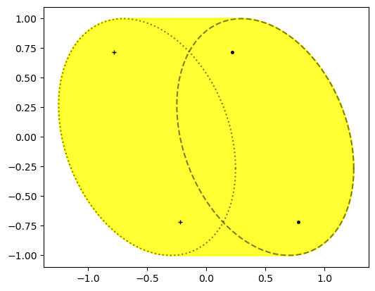
Figure 1: On the left - an example illustrating theorem 3 with $\alpha=\frac{1}{10}$, $b=1$, $b_{1}=\frac{1}{5}\left(3-i\right)$ and $b_{2}=\frac{1}{5}\left(2-i\right)$ . On the right - an example illustrating theorem 4 with $\alpha=\frac{1}{10}i$, $b=1$, $b_{1}=\frac{1}{10}\left(3+4i\right)$ and $b_{2}=\frac{1}{10}\left(4+3i\right)$ .

5 General case

We now return to arbitrary matrices (1.2), not supposing a priori the special form (3.1).

Theorem 5.

Let $A$ be of the form (1.2), with the usual convention $\beta=-\alpha$. Then $W(A)$ is bi-elliptical if and only if
(i) there exists $\theta$ for which $e^{-i\theta}C-e^{i\theta}D^{*}$ is a scalar multiple of a unitary matrix while $(e^{-i\theta}C-e^{i\theta}D^{*})D$ is not normal, and
(ii) for this value of $\theta$,

$$\quad 4\sqrt{\det\left(\operatorname{Im}(e^{-i\theta}A)\right)}(\sigma_{1}(\theta)+\sigma_{2}(\theta))^{2}=(s_{1}(\theta)-s_{2}(\theta))^{2}.$$ (5.1)

Here $\pm\sigma_{1}(\theta),\pm\sigma_{2}(\theta)$ are the eigenvalues of $e^{-i\theta}A$ (so that $\sigma_{j}(0)=\sigma_{j}$, $j=1,2$) and $s_{1}(\theta),s_{2}(\theta)$ are the non-repeating eigenvalues of $\operatorname{Im}\left((e^{-i\theta}A)^{2}\right)$.

It will become clear from the proof of Theorem 5 that $\theta$ satisfying condition (i) is unique $\mod\pi$. Also, if (i) holds then the eigenvalues $\pm\lambda_{1}(\theta),\pm\lambda_{2}(\theta)$ of $\operatorname{Im}(e^{-i\theta}A)$ actually satisfy $\lambda_{1}(\theta)=\lambda_{2}(\theta)$ and, if (ii) also holds, then $\theta=\arg(\sigma_{1}+\sigma_{2})\mod\pi$. So, with an appropriate choice of the signs condition (5.1) can be rewritten as

$$\left(\lambda_{1}(\theta)+\lambda_{2}(\theta)\right)\left(\sigma_{1}(\theta)+\sigma_{2}(\theta)\right)=s_{1}(\theta)-s_{2}(\theta).$$

Finally, condition $s_{1}(\theta)\neq s_{2}(\theta)$ follows from $(e^{-i\theta}C-e^{i\theta}D^{*})D$ not being normal.

Proof.

To establish necessity of (i), choose $e^{i\theta}$ as the direction of the line segments on $\partial W(A)$, as guaranteed by Proposition 1. The matrix $\operatorname{Im}(e^{-i\theta}A)$ then must have repeated eigenvalues. According to Lemma 1(ii), this happens if and only if the 2-by-2 hermitian matrix defined by (2.2) has coinciding eigenvalues, and is therefore a scalar multiple of the identity. This, in turn, is equivalent to $e^{-i\theta}C-e^{i\theta}D^{*}$ being a scalar multiple of a unitary matrix.

This scalar multiple cannot be zero, since otherwise $Z=e^{2i\theta}C^{*}C$ while $H=2C^{*}C$, and so $Z$ is a normal matrix commuting with $H$. As was already mentioned in the proof of Theorem 2, this situation corresponds to $W(A)$ being the convex hull of two concentric ellipses, and thus leads to a contradiction.

Both condition (5.1) and the shape of $W(A)$ persist under scaling of $A$. So, we may for the rest of the proof suppose that $\theta=0$ and $C^{*}-D=2W$ where $W$ is unitary. Furthermore, a unitary similarity of $A$ via $\operatorname{diag}[I,W]$ leaves condition (5.1) invariant, while replacing $C$ by $C_{1}=CW$ and $D$ by $D_{1}=W^{*}D$. Since $C_{1}^{*}-D_{1}=W^{*}(C^{*}-D)=2I$, it suffices to consider the case $W=I$.

This brings us into the setting of Theorem 2, with $B=D_{1}+I(=C_{1}^{*}-I)$. Since this $B$ is (or is not) normal simultaneously with $(e^{-i\theta}C-e^{i\theta}D^{*})D$, condition (i) is indeed necessary.

Supposing that (i) holds, it only remains to show that (5.1) with $\theta=0$ is (3.3) in disguise. But indeed, for $A$ as in (3.1):

$$1+v^{2}=\sqrt{\det(\operatorname{Im}A)},$$

while $\operatorname{Im}(A^{2})$ is the direct sum of two copies of $\operatorname{Im}(\alpha^{2})I+2\operatorname{Im}B$, and so $s_{1}(0)-s_{2}(0)=2(\beta_{1}-\beta_{2})$. ∎

Example. Let

$$A=\begin{bmatrix}4&0&4-8i&0\\ 0&4&5-5i&4-12i\\ -2+6i&5-5i&-4&0\\ 0&2+6i&0&-4\end{bmatrix}.$$

The matrix $e^{-i\theta}C-e^{i\theta}D^{*}$ is upper triangular, and so it can be normal only if its lower left entry is also zero. This requirement is equivalent to $\theta=-\pi/4\mod\pi$. On the other hand, with this choice of $\theta$ indeed $e^{-i\theta}C-e^{i\theta}D^{*}=\pm 10\sqrt{2}I$ is a scalar multiple of a unitary matrix (in this case, even the identity). Moreover, since $D$ is not normal, the product $(e^{-i\theta}C-e^{i\theta}D^{*})D$ is not normal either. So, condition (i) of Theorem 5 holds.

Furthermore, since

$$e^{i\pi/4}A=\sqrt{2}\begin{bmatrix}2+2i&0&6-2i&0\\ 0&2+2i&5&8-4i\\ -4+2i&5&-2-2i&0\\ 0&-2+4i&0&-2-2i\end{bmatrix},$$

somewhat lengthy but direct computations yield: $\sigma_{1}(-\pi/4)+\sigma_{2}(-\pi/4)=5\sqrt{2}$, $s_{1}(-\pi/4)-s_{2}(-\pi/4)=20\sqrt{29}$, and $\sqrt{\det\left((\operatorname{Im}(e^{i\pi/4}A)\right)}=58$. So, condition (ii) of Theorem 5 also holds, and $W(A)$ is bi-elliptical.

Figure 2: The numerical range of $A$ from the Example.

The bi-elliptical shape of $W(A)$ in the setting of Theorem 5 means that in fact $W(A)=W(A_{1}\oplus A_{2})$, where $A_{1}=-A_{2}\in\mathbb{C}^{2\times 2}$, $\sigma(A_{1})=\{\sigma_{1},\sigma_{2}\}$, and $\left\|A_{1}\right\|_{F}^{2}=\left\|A\right\|_{F}^{2}/2$. The following observation is therefore non-trivial and thus of some interest.

Proposition 6.

Any matrix (1.2) satisfying condition (i) of Theorem 5 is unitarily irreducible.

In what follows, denote by $\mathcal{L}_{\pm}$ the span of $e_{1},e_{2}$ (resp., $e_{3},e_{4}$) — the first/last two standard basis vectors of $\mathbb{C}^{4}$. The following auxiliary statement will be used repeatedly.

Lemma 2.

Let a reducing subspace $\mathcal{L}$ of the matrix (3.1) have a non-trivial intersection with $\mathcal{L}_{+}$ or $\mathcal{L}_{-}$. Then $\mathcal{L}=\mathbb{C}^{4}$.

Proof.

For any $x\in\mathbb{C}^{2}$

$$A\begin{bmatrix}x\\ 0\end{bmatrix}=\begin{bmatrix}\alpha x\\ Bx-x\end{bmatrix},\quad A^{*}\begin{bmatrix}x\\ 0\end{bmatrix}=\begin{bmatrix}\overline{\alpha}x\\ Bx+x\end{bmatrix}$$

and

$$A\begin{bmatrix}0\\ x\end{bmatrix}=\begin{bmatrix}B^{*}x+x\\ -\alpha x\end{bmatrix},\quad A^{*}\begin{bmatrix}0\\ x\end{bmatrix}=\begin{bmatrix}B^{*}x-x\\ -\overline{\alpha}x\end{bmatrix}.$$

So, if for some $x\in\mathbb{C}^{2}$ the subspace $\mathcal{L}$ contains one of the vectors $\begin{bmatrix}x\\ 0\end{bmatrix}$ or $\begin{bmatrix}0\\ x\end{bmatrix}$, it also contains the other one, as well as $\begin{bmatrix}B^{*}x\\ 0\end{bmatrix}$ and $\begin{bmatrix}0\\ Bx\end{bmatrix}$. Applying this observation to $Bx$ and $B^{*}x$ in place of $x$, we conclude that $\begin{bmatrix}0\\ B^{*}x\end{bmatrix}$, $\begin{bmatrix}Bx\\ 0\end{bmatrix}$ also lie in $\mathcal{L}$, and thus

$$\mathcal{L}\supseteq\operatorname{Span}\left\{\begin{bmatrix}x\\ 0\end{bmatrix},\begin{bmatrix}Bx\\ 0\end{bmatrix},\begin{bmatrix}B^{*}x\\ 0\end{bmatrix},\begin{bmatrix}0\\ x\end{bmatrix},\begin{bmatrix}0\\ Bx\end{bmatrix},\begin{bmatrix}0\\ B^{*}x\end{bmatrix}\right\}.$$

Since $B$ is not normal, if such a non-zero $x$ exists, it cannot be an eigenvector of both $B$ and $B^{*}$. Consequently, $\operatorname{Rank}\{x,Bx,B^{*}x\}=2$, and $\mathcal{L}=\mathbb{C}^{4\times 4}$. ∎

Proof of Proposition 6. As it was shown in the proof of Theorem 5, condition (i) implies that by scaling, rotating, and unitary similarities the matrix $A$ can be put in form (3.1) with a non-normal $B$. Since these transformations preserve unitary (ir)reducibility, we only need to consider this special case. In particular, Lemma 2 is applicable.

Observe that any reducing subspace $\mathcal{L}$ of $A$ has to be invariant under

$$A^{2}=\alpha^{2}I+\operatorname{diag}[CD,DC]=(\alpha^{2}-1)I+\operatorname{diag}[B^{*}B+B-B^{*},BB^{*}+B-B^{*}],$$

and therefore under $\operatorname{Im}A^{2}$ and $\operatorname{Re}A^{2}$. This implies the invariance under $\operatorname{diag}[B^{*}B,BB^{*}]$ and $\operatorname{diag}[\operatorname{Im}B,\operatorname{Im}B]$. Equivalently, $\mathcal{L}$ is invariant under $H_{1}=\operatorname{diag}[P_{1},P_{2}]$ and $H_{2}=\operatorname{diag}[P,P]$, where $P_{1},P_{2}$ and $P$ are spectral projections of $B^{*}B,BB^{*}$ and $\operatorname{Im}B$, respectively. Note that these projections all have rank one, and $P_{1}$ does not commute with $P_{2}$, due to non-normality of $B$.

With an appropriate choice of a unitary matrix $W\in\mathbb{C}^{2\times 2}$, a unitary similarity via $\operatorname{diag}[W,W]$ can be used to put $P$ in the form $\operatorname{diag}[1,0]$, without changing the structure (3.1) of $A$. We will use the notation $\begin{bmatrix}t_{j}&\overline{\omega_{j}}\\ \omega_{j}&1-t_{j}\end{bmatrix}$ for the resulting form of $P_{j}$, $j=1,2$. Here $0\leq t_{j}\leq 1$, with $t_{j}$ not equal zero (or one) simultaneously, and $\left|\omega_{j}\right|^{2}=t_{j}(1-t_{j})$.

Since $H_{2}=\operatorname{diag}[1,0,1,0]$, a non-zero $\mathcal{L}$ has to contain a non-zero vector $x$ of the form $[m,0,n,0]^{T}$ or $[0,m,0,n]^{T}$. If only one of $m,n$ is non-zero, Lemma 2 implies that $\mathcal{L}=\mathbb{C}^{4}$. So, we need now only to consider $m,n\neq 0$. The two options for the location of the non-zero entries can be treated similarly, and for the sake of definiteness we will assume that $x=[m,0,n,0]^{T}$.

Applying $H_{1}$ and then $H_{2}$ we see that

$$\quad[t_{1}m,\omega_{1}m,t_{2}n,\omega_{2}n]^{T},\ [t_{1}m,0,t_{2}n,0]^{T}\in\mathcal{L}.$$ (5.2)

If $t_{1}\neq t_{2}$, comparing the second vector from (5.2) with $x$ we conclude that $e_{1}$ or $e_{3}$ lies in $\mathcal{L}$. We can thus invoke Lemma 2 again.

It remains to consider the case $t_{1}=t_{2}$. The second inclusion in (5.2) is then redundant while the first can be simplified to $y=[0,\omega_{1}m,0,\omega_{2}n]^{T}\in\mathcal{L}$.

Since $\mathcal{L}$ is also invariant under $\operatorname{Im}A=\begin{bmatrix}vI&-iI\\ iI&-vI\end{bmatrix}$, along with $x,y$ it will contain $\tilde{x}=[vm-in,0,im-vn,0]^{T}$ and $\tilde{y}=[0,v\omega_{1}m-i\omega_{2}n,0,i\omega_{1}m-v\omega_{2}n]^{T}$. So, $\dim\mathcal{L}\geq\operatorname{Rank}\{x,\tilde{x},y,\tilde{y}\}=\operatorname{Rank}\Delta_{1}+\operatorname{Rank}\Delta_{2}$, where

$$\Delta_{1}=\begin{bmatrix}m&vm-in\\ n&im-vn\end{bmatrix},\quad\Delta_{2}=\begin{bmatrix}\omega_{1}m&\omega_{1}vm-i\omega_{2}n\\ \omega_{2}n&i\omega_{1}m-\omega_{2}vn\end{bmatrix}.$$

But $\det\Delta_{1}=i(m^{2}+n^{2})-2vmn$ and $\det\Delta_{2}=i(\omega_{1}^{2}m^{2}+\omega_{2}^{2}n^{2})-2\omega_{1}\omega_{2}vmn$ cannot both equal zero unless $\omega_{1}=\omega_{2}$. This, however, is precluded by non-commutativity of $P_{1}$ with $P_{2}$. So, $\mathcal{L}$ is at least 3-dimensional, it therefore has a non-trivial intersection with 2-dimensional $\mathcal{L}_{\pm}$, and yet another application of Lemma 2 completes the proof. ∎

6 Reciprocal matrices

To illustrate the applicability of Theorem 5, let us consider a so called reciprocal 4-by-4 matrix. By definition this is a tridiagonal matrix with the off-diagonal pairs of mutually inverse entries:

$$\quad A=\begin{bmatrix}0&a_{1}&0&0\\ a_{1}^{-1}&0&a_{2}&0\\ 0&a_{2}^{-1}&0&a_{3}\\ 0&0&a_{3}^{-1}&0\end{bmatrix}.$$ (6.1)

A diagonal unitary similarity can be used to change the argumets of $a_{j}$ independently, without any effect on $W(A)$. So, without loss of generality it suffices to consider matrices (6.1) with $a_{j}>0$ for all $j=1,2,3$.

Formally speaking, reciprocal matrices are not of the type considered in this paper. However, by a transpositional similarity (6.1) can be put in the form (1.2) with $\alpha=\beta=0$ and

$$\quad C=\begin{bmatrix}a_{1}&0\\ a_{2}^{-1}&a_{3}\end{bmatrix},\quad D=\begin{bmatrix}a_{1}^{-1}&a_{2}\\ 0&a_{3}^{-1}\end{bmatrix}.$$ (6.2)

This observation, combined with [6, Lemma 2.2], was used in K. Vazquez’s Capstone project (under the supervision of one of the authors) to obtain the criterion for the matrix (6.1) to have an elliptical numerical range. A similar result was obtained simultaneously and independently by N. Bebiano and J. da Providéncia (private communication). Stated in terms of

$$\quad A_{j}=\frac{a_{j}^{2}+a_{j}^{-2}}{2}\ (\geq 1),$$ (6.3)

this criterion looks as follows:

$$A_{2}=\frac{1+\sqrt{5}}{2}A_{1}+\frac{1-\sqrt{5}}{2}A_{3}\text{ or }A_{2}=\frac{1+\sqrt{5}}{2}A_{3}+\frac{1-\sqrt{5}}{2}A_{1},$$

and at least one of the inequalities in (6.3) is strict.

Here is what follows for reciprocal matrices (6.1) by applying Theorem 5 to $A$ given by (1.2),(6.2) with $\alpha=\beta=0$.

Theorem 7.

Let $A$ be as in (6.1). Then $W(A)$ is bi-elliptical if and only if $A_{1}=A_{3}>1$ (equivalently: $a_{1}=a_{3}\neq 1$ or $a_{1}=a_{3}^{-1}\neq 1$) and $A_{2}=1$ (equivalently: $a_{2}=1$).

Proof.

With $C$ and $D$ given by (6.2), the matrix $Z$ from (2.1) is simply

$$Z=\begin{bmatrix}2&a_{2}a_{3}\\ a_{2}^{-1}a_{3}^{-1}&1\end{bmatrix}.$$

So, the eigenvalues $z_{1},z_{2}$ of $Z$ are $(3\pm\sqrt{5})/2$, and by Lemma 1(i) with $\alpha=0$ the spectrum of $A$ consists of the four point $\pm(1\pm\sqrt{5})/2$.

The only candidates for $\theta$ in the statement of Theorem 5 in our setting are therefore integer multiples of $\pi$.

With this choice of $\theta$, the matrix $e^{-i\theta}C-e^{i\theta}D^{*}$ up to the sign equals

$$C-D^{*}=\begin{bmatrix}a_{1}-a_{1}^{-1}&0\\ a_{2}^{-1}-a_{2}&a_{3}-a_{3}^{-1}\end{bmatrix}.$$

It is a scalar multiple of a unitary if and only if $a_{2}^{-1}-a_{2}=0$ and $a_{1}-a_{1}^{-1}=\pm(a_{3}-a_{3}^{-1})$. These are exactly the conditions $A_{2}=1$, $A_{1}=A_{3}$.

Finally, with $a_{2}=1$ the matrix

$$(C-D^{*})D=\begin{bmatrix}1-a_{1}^{-2}&a_{1}-a_{1}^{-1}\\ 0&1-a_{3}^{-2}\end{bmatrix}$$

is normal if and only if $a_{1}=1$ (equivalently: $A_{1}=1$). This concludes the proof of necessity.

To prove sufficiency, we just need to show that (5.1) holds with $\theta=0$. To this end, observe that

$$\det(\operatorname{Im}A)=\frac{1}{16}\left|\det(C-D^{*})\right|^{2}=\frac{1}{16}(a_{1}-a_{1}^{-1})^{2}(a_{3}-a_{3}^{-1})^{2}=\frac{1}{4}(A_{1}-1)^{2},$$

and $\operatorname{Im}(A^{2})$ is unitarily similar to $\operatorname{Im}Z\oplus\operatorname{Im}Z$ so that $s_{1,2}=\pm(a_{3}-a_{3}^{-1})/2$. Consequently,

$$(s_{1}-s_{2})^{2}=(a_{3}-a_{3}^{-1})^{2}=2A_{3}-2=2A_{1}-2.$$

We see that (5.1) indeed holds if we pick $\sigma_{1,2}\in\sigma(A)$ as say $(1\pm\sqrt{5})/2$. ∎

Figure 3: An example illustrating Theorem 7 with $A_{2}=1$ and $A_{1}=A_{3}=3$.

References

- [1] E. Brown and I. Spitkovsky, On flat portions on the boundary of the numerical range, Linear Algebra Appl. 390 (2004), 75–109.
- [2] M. T. Chien and K.-C. Hung, Elliptical numerical ranges of bordered matrices, Taiwanese J. Math. 16 (2012), no. 3, 1007–1016.
- [3] U. Daepp, P. Gorkin, A. Shaffer, and K. Voss, Finding ellipses, Carus Mathematical Monographs, vol. 34, MAA Press, Providence, RI, 2018, What Blaschke products, Poncelet’s theorem, and the numerical range know about each other.
- [4] H.-L. Gau, Elliptic numerical ranges of matrices, Taiwanese J. Math. 10 (2006), no. 1, 117–128.
- [5] H.-L. Gau and P. Y. Wu, Line segments and elliptic arcs on the boundary of a numerical range, Linear Multilinear Algebra 56 (2008), no. 1-2, 131–142.
- [6] T. Geryba and I. M. Spitkovsky, On the numerical range of some block matrices with scalar diagonal blocks, Linear Multilinear Algebra (2020).
- [7] R. A. Horn and C. R. Johnson, Topics in matrix analysis, Cambridge University Press, Cambridge, 1994, Corrected reprint of the 1991 original.
- [8] D. Keeler, L. Rodman, and I. Spitkovsky, The numerical range of matrices, Linear Algebra Appl. 252 (1997), 115–139.
- [9] R. Kippenhahn, Über den Wertevorrat einer Matrix, Math. Nachr. 6 (1951), 193–228.
- [10] , On the numerical range of a matrix, Linear Multilinear Algebra 56 (2008), no. 1-2, 185–225, Translated from the German by Paul F. Zachlin and Michiel E. Hochstenbach.
- [11] Y. T. Yeh, Numerical range of 2-by-2 block matrices, Master’s thesis, National Central University, Taiwan, 2011.