A QUBO formulation for qubit allocation

Abstract

To run an algorithm on a quantum computer, one must choose an assignment from logical qubits in a circuit to physical qubits on quantum hardware. This task of initial qubit placement, or qubit allocation, is especially important on present-day quantum computers which have a limited number of qubits, connectivity constraints, and varying gate fidelities. In this work we formulate and implement the qubit placement problem as a quadratic, unconstrained binary optimization (QUBO) problem and solve it using simulated annealing to obtain a spectrum of initial placements. Compared to contemporary allocation methods available in t$\mid$ket$\rangle$ and Qiskit, the QUBO method yields allocations with improved circuit depth for $>$50% of a large set of benchmark circuits, with many also requiring fewer CX gates.

I Introduction

The past decade has seen significant development in quantum computing hardware, with a number of commercially-available machines and software libraries that enable users to program and execute their own quantum algorithms. While architectures and implementations vary, common issues with present-day machines are the limited qubit connectivity and high error rates, especially for two-qubit operations.

A crucial underlying part of the quantum software stack is the process of quantum compilation, which includes circuit synthesis and optimization, transpilation, initial placement, and qubit routing. Initial placement, or qubit allocation, is the process that assigns logical qubits in a quantum circuit to physical qubits on the quantum hardware graph. This must be done taking into account a variety of factors: error rates, number of operations, operation times, decoherence times, and connectivity all play a role in determining the quality and success of a quantum algorithm.

The problem of qubit allocation, however, is NP-complete Siraichi et al. (2018). While for small cases we can simply test every possible allocation and determine the one with, e.g. the highest success probability, or the fewest SWAPs to work around connectivity, for larger circuits and devices one must design effective techniques to choose the allocation. This problem has garnered significant attention lately, with a variety of approaches considered Tan and Cong (2020a); Dueck et al. (2018); Li et al. (2020); Ghosh et al. (2020); Deng et al. (2020); Zhang et al. (2020); Childs et al. (2019); Zulehner and Wille (2019); Brierley (2015); Paler (2019); Paler et al. (2020); Nash et al. (2020); Lin et al. (2019); Smith et al. (2020a); Webber et al. (2020) and incorporated in a number of full-stack toolkits Amy and Gheorghiu (2020); Smith et al. (2020b); Sivarajah et al. (2020); et al. (2019); Google (2019). Some common techniques involve partitioning of the circuit into blocks, finding the optimal assignment within each block, and then swapping qubits between blocks to satisfy the connectivity constraints Wille et al. (2019); Li et al. (2019); Cowtan et al. (2019); Pedram and Shafaei (2016). Other approaches use machine-learning techniques to optimize circuit synthesis Herbert and Sengupta (2018); Pozzi et al. (2020). Recently, a number of methods have focused on incorporating hardware calibration data in an effort to improve the final circuit fidelities Murali et al. (2019); Wilson et al. (2020); P. Jurcevic et al. (2020); Nishio et al. (2020); Tannu and Qureshi (2018); Bhattacharjee et al. (2019) .

A handful of approaches have also considered simulating annealing Finigan et al. (2018); Zhou et al. (2020). Simulated annealing is a widely-applied heuristic optimization technique that involves randomly choosing an initial configuration, and allowing the system to transition between states with some probability in order to find a global minimum. In this work, we apply simulated annealing to the qubit allocation problem formulated specifically as a quadratic, binary unconstrained optimization problem, or QUBO.

The QUBO formulation is familiar to the quantum computing community due to its equivalence to the two-dimensional Ising model, and its use as the basis for the optimization problems solvable by D-Wave’s quantum annealers and Fujitsu’s digital annealers. A cost function for a QUBO problem can be expressed in the form:

$$\min_{x}\sum_{ij}\sum_{k\ell}Q_{ijk\ell}x_{ij}x_{k\ell}+\sum_{ij}b_{ij}x_{ij}+\hbox{constraints},$$ (1)

where $x_{ij}$ are binary variables for which we would like to find an assignment, and $Q_{ijkl}$ and $b_{ij}$ are coefficients that incorporate information about relationships between them. The aim is to find an assignment of $x_{ij}$ such that the above cost, or ‘energy’, is minimized. For qubit allocation we use the $x_{ij}$ to indicate the decision to assign logical qubit $i$ to hardware qubit $j$ ($x_{ij}=1$ if true, $x_{ij}=0$ if not). The quadratic terms $Q_{ijkl}$ carry information about the quality of choosing, in the same assignment, to map logical qubit $i$ to hardware qubit $j$, and $k$ to $\ell$. Similarly, the linear terms are based on the quantity and quality of single-qubit operations. Constraints are added to ensure unique assignment of each logical qubit to a single hardware qubit.

The QUBO method coupled with simulated annealing demonstrated a number of distinct advantages compared to existing initial allocation methods. The method was found to be incredibly flexible in terms of cost-function design. For example, including a specific metric (e.g. success probability) within the QUBO cost function results in higher quality allocations with respect to that metric. Simulated annealing also enables one to generate thousands of solutions for relatively low computational cost. Having access to these distributions of initial allocations allowed us to investigate the allocation process in more detail, as we could look at where logical qubits tended to be allocated on the hardware graph. Finally, the computational requirements are agnostic to the structure of the circuit, and essentially limited by only the time-scaling of simulated annealing. The largest circuits we tested were on a 53-qubit hardware graph, with 1000 allocations obtained in 30 minutes (2 seconds per allocation), making this method appealing for the next generations of NISQ devices that will have in the range of 50-100 qubits.

In Section II, we discuss QUBOs, our choice of coefficients, and the metrics by which we gauge the quality of our solutions. In Section III we analyze the performance of our method using a benchmark circuit set, and provide details about our implementation, which we note is available open-source on our Github git . Section IV compares the solution quality of the QUBO formulation to that of other contemporary software tools — Qiskit et al. (2019) and t$\mid$ket$\rangle$ Sivarajah et al. (2020) — as well as the recently published QUEKO benchmarks Tan and Cong (2020b) to investigate the optimality gap of QUBO allocations. We conclude in Section V by suggesting a number of interesting possible extensions of this method.

II A QUBO for qubit allocation

II.1 QUBO formalism

A quadratic unconstrained binary optimization problem, or QUBO, is generally defined as

$$\min_{x}\enskip x^{T}Qx$$ (2)

where $x$ is an $N$-dimensional vector of binary variables and $Q\in\mathbb{R}^{N\times N}$. The QUBO model can represent a variety of problems in the field of combinatorial optimization (CO) such as max-cut, set partitioning, graph-colouring, and quadratic assignment Kochenberger et al. (2014). An excellent tutorial paper on the formulation of QUBO models for problems like these is available in Glover et al. (2018). In particular, the QUBO model is equivalent to the Ising model up to a linear transformation, allowing many problems in the physics domain to be recast in it as well Lucas (2014); Lodewijks (2019).

A particular strength is that once a problem is reformulated as a QUBO, it can be solved without using a method specialized to the domain of the problem, and usually produces solutions whose quality rivals that of the specialized methods. As discussed in Subsection III.1, we use simulated annealing, but there are many other choices (see, for example, the methods summarized in sections 7 and 8 in Burkard (2013)).

Qubit allocation is an instance of the quadratic assignment problem, meaning our binary variables indicate whether or not to make a particular assignment of logical to physical qubits. To be explicit,

$$x_{ij}=\begin{cases}1&\mbox{assign logical qubit }i\hbox{ to hardware qubit }j\\ 0&\mbox{otherwise }\end{cases}$$

The problem we now must solve is to find an assignment of logical to physical qubits that minimizes the cost function. To do so we must choose suitable coefficients (Subsection II.2) and enforce any required constraints (Subsection II.3).

II.2 QUBO coefficients

In Equation 2, the coefficients in $Q$ represent relationships between the binary variables. For qubit allocation, these coefficients should depend on the properties of the circuit in question, and the hardware graph on which we are performing the computation. The particular form is flexible, and it is an important and defining decision to choose the information and metrics upon which they are created.

QUBO cost functions are often re-expressed as a summation:

$$\min_{x}\sum_{ijkl,ij\neq kl}Q_{ijkl}x_{ij}x_{kl}+\sum_{ij}b_{ij}x_{ij}.$$ (3)

The first set of terms are quadratic terms, and their value will relate to the quality of assigning logical qubit $i$ to hardware qubit $j$, and logical qubit $k$ to hardware qubit $l$ in the same allocation. The diagonal terms of this sum have been removed and re-written as linear terms (since $x_{ij}^{2}=x_{ij}$ for binary variables). The linear terms pertain to the assignments ‘in isolation’, meaning just the consequences of assigning logical qubit $i$ to hardware qubit $j$.

As the QUBO expression represents a cost, the coefficients must be chosen such that minimization of Equation 3 is meaningful. Given a circuit and hardware graph, we focus on the number and type of one and two qubit gates, the error-rates of the hardware, and the connectivity of the hardware. Roughly, the coefficients are a product:

$$f_{\hbox{error}}(\varepsilon)\times f_{\hbox{gate}}(g)\times f_{\hbox{dist}}(d)$$ (4)

where $\varepsilon$ is some function of error rates (in our case, we use the success probability), $g$ a number of gates, and $d$ a distance. The functions $f_{\hbox{gate}},f_{\hbox{error}}$, and $f_{\hbox{dist}}$ are then to be determined. A variety of coefficient forms were tested to determine one that yielded the best results according to a set of metrics: the number of added SWAPs, and the success probability of the final circuit (including any added SWAPs). These are discussed in detail in Subsection III.1.

II.3 Handling constraints

The form in Equation 3 doesn’t explicitly account for constraints on the variables. For the qubit allocation problem - and quadratic assignment problem in general - allocations that assign the same logical qubit to multiple hardware qubits (as well as assignments of multiple logical qubits to a given hardware qubit) are not valid allocations. Mathematically, this is expressed as:

$$\sum_{i=1}^{n_{c}}x_{ij}=1\qquad j=1,...,n_{p}$$ (5)

$$\sum_{j=1}^{n_{p}}x_{ij}=1\qquad i=1,...,n_{c}$$ (6)

where $n_{c}$ is the number of logical qubits and $n_{p}$ is the number of available hardware (physical) qubits. In other words, the qubit mapping must be bijective (i.e. a one-to-one mapping). Visually this can be seen in Figure 1, where no row or column sees more than one allocation.

Figure 1: An example of a valid allocation for a 12-qubit circuit to a 15-qubit hardware graph. Yellow squares represent an allocated qubit ($x_{ij}=1$). The constraints of the problem prevent having more than one allocation within a row and column (no under or over assignments of qubits).

Constraints are incorporated by adding penalty terms to the QUBO:

$$\phi\left(\sum_{i=1}^{n_{c}}x_{ij}-1\right)^{2},\qquad j=1,...,n_{p}$$ (7)

$$\theta\left(\sum_{j=1}^{n_{p}}x_{ij}-1\right)^{2},\qquad i=1,...,n_{c}$$ (8)

These terms are designed such that for a constraint-violating solution they produce a positive value (thus increasing the cost), but evaluate to 0 if the constraints are satisfied. Here $\phi$ and $\theta$ are penalty coefficients. These coefficients control the relative tendency of the optimizer to want to minimize the cost of Equation 2 versus satisfying the constraints. The specific choice of these coefficients will be discussed in Subsection III.2. Adding the constraints to Equation 3 yields:

$$\sum^{n_{c}}_{\begin{subarray}{c}i=1\\ i\neq k\end{subarray}}\sum^{n_{p}}_{\begin{subarray}{c}j=1\\ j\neq l\end{subarray}}\sum^{n_{c}}_{k=1}\sum^{n_{p}}_{l=1}Q_{ijkl}x_{ij}x_{kl}+\sum^{n_{c}}_{i=1}\sum^{n_{p}}_{j=1}(b_{ij}-(\phi+\theta))x_{ij}$$ (9)

as the full QUBO for qubit allocation.

III Implementation details

We implemented our methods in Python, and make the code available open source on our Github git . An end-to-end example can be found in a Jupyter notebook under ‘examples’ in the Github.

Simulated annealing was used to find the solutions to our QUBO model. Specifically, we leverage D-Wave’s neal Python package D-Wave Systems Inc. (2020), as it has built-in support for QUBO applications. Simulated annealing allows us to easily produce distributions of allocations by performing multiple anneals. This will produce allocations of varying quality, and enables us to see which properties of an initial allocation actually end up mattering for the compiled circuit. In this context, quality refers to how good the final properties of a fully routed circuit are, as a function of the initial allocation. The success metrics considered are the number of SWAPs after routing, and the success probability of the final routed circuit.

III.1 Choosing QUBO coefficients

As per Equation 4, we would like to construct coefficients that incorporate information about the number of gates, distance between qubits on the hardware graph, and error rates of the gates. To that end, for the linear terms we would like a coefficient with the form:

$$b_{ij}=f_{\hbox{error}}(p_{j})\cdot f_{\hbox{gate}}(g_{i})$$ (10)

where $g_{i}$ is the number of single-qubit gates acting on qubit $i$, and $p_{j}$ is the success probability for a single qubit gate on hardware qubit $j$. For the quadratic terms, we suppose:

$$Q_{ijk\ell}=f_{\hbox{error}}(p_{j\ell})\times f_{\hbox{gate}}(g_{ik})\times f_{\hbox{dist}}(d_{j\ell}).$$ (11)

Here $g_{ik}$ is the number of two-qubit gates acting on logical qubits $i$ and $k$. The value of $p_{j\ell}$ is the success probability of executing a two-qubit gate between hardware qubits $j$ and $\ell$ (accounting for any SWAPs that must be added). Finally $d_{j\ell}$ is the minimum distance between hardware qubits $j$ and $\ell$ on the hardware graph. We note that the functions $f$ need not be the same between Equation 10 and Equation 11.

Computing $p_{j}$ and $g_{i}$ for the single qubits is straightforward. For the two-qubit gates, the coefficients must take into account that for two-qubit gates between hardware qubits that are not connected, SWAPs must be inserted to satisfy these constraints. This affects how the value of $p_{j\ell}$ is calculated. In an effort to investigate the quality of just the initial allocation and not the subsequent circuit synthesis and routing process, we ‘naively’ calculate SWAP counts as to not rely on any specific compiler. For each two-qubit gate that requires at least one SWAP, we calculate the smallest number of SWAPs that must be added, and assume the qubits are swapped back immediately afterwards. This number of SWAPs is then used to compute the success probability of a given two-qubit operation.

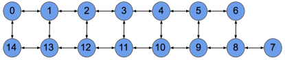
Figure 2: Architecture graph for IBM Melbourne, a 15-qubit quantum computer. Edges between nodes indicate qubit connectivity, where each edge is bidirected (can support a CX gate in either direction).

Various functions of the quantities of interest were compared using a set of 157 benchmark circuits (taken from Zulehner et al. (2018)’s Github) which range from 3-16 logical qubits. A small amount of filtering had to be performed on this set for this portion of the work. First, we chose to use the IBM Melbourne hardware graph (Figure 2), and so only circuits with up to 15 logical qubits were used. To gauge the quality of the coefficient forms, we analyzed the percentage difference in naive SWAP count, so for purposes of comparison we do not consider three circuits in which no SWAPs needed to be added. We also considered a percentage difference of success probability, however for some very large circuits (27 of them), the success probabilities were effectively 0, and these data points were also not used in the coefficient form comparison.

For each coefficient form and circuit, we performed 1000 anneals and analyzed the resulting allocations. As a first example, Figure 3 shows the distribution of costs (typically called ‘energies’) for 1000 anneals of a 7-qubit circuit (hwb6_56) with 3771 single-qubit gates and 2952 two-qubit gates, embedded on a 15-qubit hardware graph (IBM Melbourne, Figure 2). The obtained distribution of energies allows us to verify the behaviour of the QUBO cost function for different coefficient forms, and ensure that our quality metrics are well-correlated with the annealing outcomes.

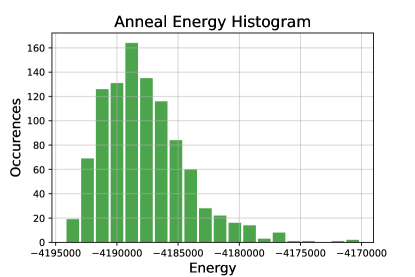
Figure 3: Histogram of 1000 anneal energies for benchmark circuit hwb6_56, using the coefficient form in Equation 14. As sample number increases, these histograms tend to approach a log-normal distribution. The general trend in energies is that for smaller circuits the plot will be very skewed towards lower energies, as the ‘best’ initial allocation (in terms of fewer added SWAPs) will be found for the majority of anneals, while for larger circuits the sample space is too large to find convergence on a particular allocation, and the energies become more normally distributed.

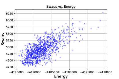
Figure 4: Comparison of SWAP count and allocation energy for a 1000 sample anneal run for benchmark circuit hwb6_56, using the coefficient form in Equation 14. SWAP count here is computed using the naive method used to generate the coefficients, without further routing. While there is significant variation, there is a general tendency for lower-energy allocations to also have lower SWAP counts, indicating that the choice of cost function is able to produce quality solutions.

One such comparison is in Figure 4, where we plot the naive SWAP counts for all allocations of a benchmark circuit (hwb6_56) against their energy for a particular run of 1000 anneals. Clearly the lower energy allocations tend to also have lower SWAP counts. This trend generally held true for all of our benchmark circuits, for both of our quality metrics.

Figure 5 presents a percentage difference comparison between two candidate forms over the benchmark set:

$$Q_{ijk\ell}=-\ln(p_{j\ell})\cdot g_{ik}\cdot d_{j\ell},\quad b_{ij}=-\ln(p_{j})\cdot g_{i},$$ (12)

versus

$$Q_{ijk\ell}=-\ln(p_{j\ell})\cdot g_{ik}\cdot d_{j\ell}^{2},\quad b_{ij}=-\ln(p_{j})\cdot g_{i}.$$ (13)

The quantities here are as defined below Equation 11. The top plot shows the percentage difference of average naive SWAPs from the top 1% of allocations for each form (i.e. the lowest energy solutions), and the bottom plot the percentage difference of naive SWAPs for the full set of allocations. For the top 1% we see that both coefficient forms find the lowest SWAP allocation for smaller circuits, but start to diverge as the number of logical qubits increases past 6, where the form with $d_{j\ell}^{2}$ clearly finds better allocations over the one with just $d_{j\ell}$. In the plot that considers the full set of allocations, there is no convergence for smaller circuits and it is apparent that the form in Equation 13 is superior for the vast majority of benchmark circuits.

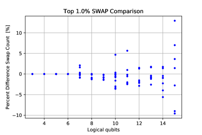
(a)

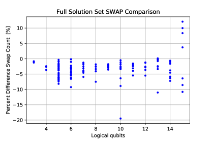
(b)

Figure 5: A comparison of the two different QUBO coefficient forms in Equation 12 and Equation 13. The quadratic coefficients differ, with one form incorporating distance as-is, while the other uses the distance squared. The plot shows the percentage difference between the two forms’ average SWAP counts (over 1000 anneals) over the set of benchmark circuits. A negative value indicates that the squared-distance coefficient form has lower SWAP counts. One sees that for the lowest energy solutions (top), the performance is comparable, with the squared-distance having a slight advantage, but for the distribution as a whole the squared-distance yields consistently lower SWAP counts.

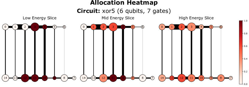
Figure 6: Heatmap showing a range of allocations to the IBM Melbourne hardware graph obtained from a 1000-sample run of simulated annealing. Each panel shows 5$\%$ of the solutions for a given energy range. Darker colour indicates a higher concentration of allocations involving that specific qubit. The node and edge sizes are proportional to one and two-qubit error rates, where bigger is better (i.e. smaller error-rates). Lower-energy (i.e. higher quality) solutions shown on the left see the allocations clustering around the most well-connected qubis with the lowest error rates, whereas higher-energy solutions are more variable.

To look deeper into the structure of the allocation process we used heatmaps, where different sets of allocations at different energies are plotted on the hardware graph to show the distribution of the qubits being assigned. In Figure 6 are heatmaps for IBM Melbourne representing the lowest 5% of the energies, the middle 5%, and the highest 5%, taken from a 1000-sample annealing run. The qubits are coloured based on the fraction of allocations within that energy range that include those qubits. The node and edge sizes are scaled based on the single and two-qubit error rates respectively, where a larger size means a better (lower) single-qubit error-rate, and thicker edges indicate better (lower) two-qubit error rates. We notice that in these examples, for low energies the allocations tend to converge on the most well-connected qubits with the lowest error-rates, dispersing as the energies increase. This is visual affirmation that lower energy allocations are better allocations, as they converge on the ‘best’ available physical qubits.

We continued testing various coefficient forms using the percentage difference comparison method (the full complement of which can be found on our Github git ) ultimately concluding that the form:

$$Q_{ijk\ell}=-\ln(p_{j\ell})\cdot g_{ik}\cdot d_{j\ell}^{3},\quad b_{ij}=-\ln(p_{j})\cdot g_{i}$$ (14)

generally performs well based on our quality metrics. It is worth noting that squaring the graph distances (as in Equation 13) actually performed better on average for smaller circuits (in terms of logical qubit number), but worse for larger circuits. Perhaps with further investigation, one could find a threshold to decide which exponent to use based on input circuit properties.

While this is the best coefficient form we found, we encourage the interested reader to investigate other forms, or other quality metrics that may better suit their purposes. In general we found that incorporating a particular metric as a part of the QUBO coefficients will improve the final solutions of the QUBO with respect to that metric. During the experimentation process we determined some good rules of thumb for this inclusion. For example, multiplying the desired metrics performed better than adding them, and allocations obtained by taking the natural log of the success probabilities produced routed circuits with higher success probabilities. We also tried re-scaling the number of one- and two-qubit gates, removing the linear term ($b_{ij}$) entirely, and using subsets of the three metrics shown in Equation 11, however none of these produced allocations with significantly better quality than Equation 14.

As a final note, one question that arises is whether correlation with energy is present after the circuit has been compiled (and thus fully routed) to insert any necessary SWAPs. A test of this is shown in Figure 7, where we take a sample of 1000 allocations from an anneal run for a 14-qubit circuit (cm42a_207) with 1005 single-qubit gates and 771 two-qubit gates, using IBM Melbourne as a hardware graph. Each allocation is given to Qiskit’s compiler (v0.20.0) using level 0 optimization and the ‘basic’ routing method, and the SWAP counts of the compiled circuits are plotted. As can be seen visually, there is no strong correlation between QUBO allocation energies and compiled circuit SWAP counts. This means that we cannot predict which QUBO initial allocation will produce the best compiled circuit.

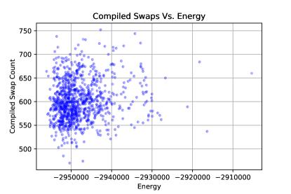
Figure 7: Distribution of Qiskit SWAP counts for each allocation in a 1000 sample anneal run for benchmark circuit cm42a_207. Compiled using Qiskit v0.20.0 using a preset passmanager with optimization level 0 and the ‘basic’ routing method. We can infer that it is not possible to predict the compiled circuit SWAP counts based on the energy of a given allocation.

It would be of particular interest to further investigate other QUBO coefficient forms that would have such predictive power. We leave this as an interesting problem for future work. We can still be confident that the lower energy QUBO allocations are better initial allocations from the fact that they are well correlated with our own quality metrics, meaning the QUBO method is self-consistent. Furthermore, comparison must also be made against other initial placement techniques to investigate if there are improvements from the QUBO allocations, as even if the compiled SWAPs are not so correlated, we may still see improvements on average. Highlights of such comparisons are made in Subsection IV.1, with the full set of results in Appendix A.

III.2 Penalty coefficients

In addition to choosing a form for $Q_{ijk\ell}$ and $b_{ij}$, we must also choose values of $\phi$ and $\theta$. This aspect is often not discussed in the literature for other QUBO applications, which simply specifies that a typical choice is 75-150% of the maximum value of the coefficient matrix without constraints added (see end of section 4.1 in Glover et al. (2018)).

We found that the above rule-of-thumb worked reasonably well, but required a small amount of tweaking. The final process for deciding penalty values consisted of first setting both $\phi$ and $\theta$ equal to the maximum coefficient matrix value. We would then check if any of the returned allocations from simulated annealing did not satisfy the constraints. If at least one was invalid, we would re-run that circuit until all the allocations satisfied the constraints, multiplying the penalties by 2, then 3, etc. on each successive run. In the course of our benchmarking, no circuit ever had to have their penalties increased beyond 3 times the maximum coefficient matrix value, with the vast majority of circuits succeeding without needing to be re-run.

As a final point of interest, we had initially included an additional constraint,

$$\gamma\left(\sum^{n}_{i=1}\sum^{n}_{j=1}x_{ij}-n_{c}\right)^{2},$$ (15)

which ensured that the correct number of qubits were assigned. The concern was that for circuits where the number of logical qubits was less than the amount of available hardware qubits, it would tend to assign more qubits than required. As it turned out, adding this additional constraint was unnecessary — the other constraints appear to implicitly handle this — and actually made it more challenging to set the penalty coefficients.

We note that given the results of some initial tests while hand-tuning penalty coefficients, it does seem like there is an optimal range for each circuit (paired with a particular coefficient form). An interesting topic of future investigation could be to automate the selection process, or employ something akin to a Newton’s method algorithm to converge on these circuit-optimal ranges.

IV Benchmarks

In this section we analyze the effectiveness of the QUBO formulation and compare its performance to other contemporary allocation methods available in t$\mid$ket$\rangle$ (pyt$\mid$ket$\rangle$ v0.5.7) Sivarajah et al. (2020) and Qiskit (v0.20.0) et al. (2019) (Subsection IV.1). In Subsection IV.2 we also analyze performance with respect to the set of recently-proposed QUEKO benchmarks Tan and Cong (2020b). All benchmarks were run on a machine with an Intel i5-4590 4-core processor at 3.30 GHz with 16 GB of RAM.

IV.1 Comparison against contemporary initial placement methods

Using the benchmarks available at Zulehner et al. (2018)’s Github, the performance of our method was compared to initial allocation methods available in t$\mid$ket$\rangle$ and Qiskit. We also compare with the initial allocation method used by the SABRE algorithm Li et al. (2019), which was recently added to Qiskit.

For these benchmarks, we use IBM Melbourne (see Figure 2) as our hardware-graph, and for each circuit we take the QUBO allocation with the lowest naive-SWAP count. As we care primarily about the performance of the initial allocation, we specifically turn off all further circuit synthesis optimization so that the Qiskit and t$\mid$ket$\rangle$ compilers are essentially just routing the mapped circuits. For Qiskit, this corresponds to using the level 0 optimization preset passmanager with the ‘basic’ router. For t$\mid$ket$\rangle$ we set all routing parameters available in the router function (swap_lookahead, bridge_lookahead, bridge_interactions, bridge_exponent) to 0 and didn’t apply any further optimization calls.

Before calculating any of the compiled circuit’s properties, we decompose all SWAP gates to CX gates (for t$\mid$ket$\rangle$ we also decompose all BRIDGE gates). To assess the quality of the initial allocation, we compute the total number of CX gates and the circuit depth for the routed circuit, as these are (generally) the metrics that most other qubit allocation methods report.

As for our choice of benchmark circuits, since we are allocating to a 15-qubit hardware, we must ignore 6 of the 157 benchmark circuits due to them using 16 logical qubits, leaving us with 151 benchmarks. For t$\mid$ket$\rangle$ we use all 151 remaining benchmarks, but for Qiskit we restrict ourselves to using only circuits with 10,000 or fewer total gates, due to poor time-scaling for very large circuits. With this restriction in place, we are left with 131 benchmark circuits for comparison with Qiskit. The detailed results are included in Appendix A for both compilers. In this section we discuss the highlights.

Allocation Method	CX count [%]	Depth [%]
LinePlacement	56.9	58.9
GraphPlacement	55.0	59.0
Trivial	90.1	85.1
Dense	68.6	70.2
Noise	57.9	77.0
SABRE	48.8	53.7

Table 1: Table showing the percentage of total benchmark circuits for which QUBO demonstrated improvement over the specified allocation methods, for both performance metrics (total CX count and circuit depth). The first two methods are from t$\mid$ket$\rangle$ and the subsequent four from Qiskit.

For t$\mid$ket$\rangle$ we compare to the LinePlacement and GraphPlacement initial allocation methods. For Qiskit we compare to the Trivial, Dense, Noise and SABRE allocation methods. In Table 1 we present the overall performance of the QUBO method in terms of the percentage of benchmark circuits in which it yielded improvement over the other initial placement methods. Notably, QUBO finds a better allocation for $>$50% of the benchmark circuits compared to almost every other allocation method, in terms of CX count and circuit depth. The single exception is that the SABRE placement technique more often yields better CX counts. While this big picture result is valuable, we must analyze the performance on a more fine-grained level.

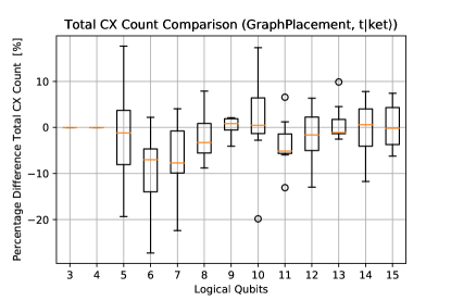
Figure 8: Box plot of the percent difference comparison between the t$\mid$ket$\rangle$ GraphPlacement initial allocation method and the QUBO lowest SWAP allocation for total CX count, over all applicable benchmark circuits. The difference is taken such that a negative value indicates that the QUBO-obtained allocations required fewer added CX gates.

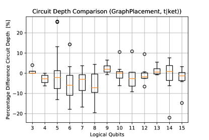
Figure 9: Box plot of the percent difference in circuit depth between the t$\mid$ket$\rangle$ GraphPlacement initial allocation method and the QUBO lowest naive-SWAP allocation over all applicable benchmark circuits. A negative value indicates that the QUBO-obtained allocations had a lower circuit depth.

To compare the initial allocation’s compiled circuit properties (total CX count and circuit depth) we again employ percent-difference comparisons, plotting the results as box-and-whisker plots as a function of logical qubit number. Figure 8 and Figure 9 show the comparison between the QUBO method and the t$\mid$ket$\rangle$ GraphPlacement method for total CX count and circuit depth, respectively. The overall performance of both methods is fairly circuit dependent, but the distributions seem to be skewed in QUBO’s favour, especially for smaller circuits. In the smallest circuits (four or fewer logical qubits) both methods converge on the same CX counts, but still differ slightly in circuit depth, with a very slight edge to QUBO. While we don’t show here a percentage difference comparison between LinePlacement and QUBO (it is available on our Github git ) we note that it is fairly similar to the GraphPlacement comparison, with the only notable difference being that for two of circuits, the QUBO allocation obtained much lower depth and CX count ($>$55% difference for depth, $>$40% difference for CX count). We also note that the GraphPlacement method was significantly slower at finding allocations compared to both LinePlacement and QUBO, taking several minutes for some circuits in this benchmark set, and in some cases hours for some circuits in the to-be-discussed QUEKO B_SS benchmark set (see Subsection IV.2 for more detail.)

For comparison with Qiskit, the methods of interest are the Dense and SABRE allocation methods. Qiskit also contains two additional methods, Trivial and Noise, but Noise performs similarly to Dense, and unsurprisingly the Trivial method performs poorly compared to all the other methods.

In Figure 10 and Figure 11, we can see the comparison between QUBO and Dense. Looking at the distributions, most are skewed in favour of the QUBO allocation, partly due to some outlier circuits where QUBO performed significantly better than Dense. We see again that the QUBO allocations are more favourable for the smaller circuits in the benchmark set than the larger ones, but this is more likely to be a function of the gate compositions of the circuits than a function of logical qubit number, given that we see such large variation for particular logical qubit numbers.

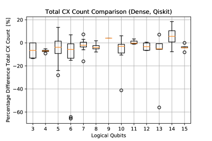
Figure 10: Box plots of the percent difference comparison in total CX count between Qiskit’s Dense initial allocation method and the QUBO lowest naive-SWAP allocation over all applicable benchmark circuits. A negative value indicates that QUBO allocations had fewer CX gates added.

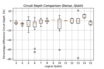
Figure 11: Box plots of the % difference comparison between Qiskit’s Dense initial allocation method and the QUBO lowest SWAP allocation for circuit depth, over all applicable benchmark circuits. The difference is taken such that a negative value indicates that QUBO allocations had smaller depths.

In Figure 12 and Figure 13 we compare QUBO and SABRE. Again we see some large outlier circuits for which QUBO does significantly better. In terms of the distributions of percent differences, both QUBO and SABRE seem to perform equally well for smaller circuits, with a slight edge to QUBO for the medium sized circuits and to SABRE for the larger circuits. This is more pronounced in the depth plot, where there is a clear dip in the middle. SABRE seems to also do a slightly better job at finding smaller depths than QUBO.

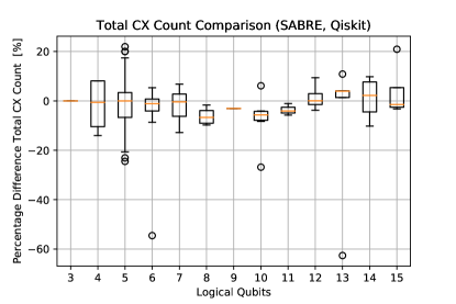
Figure 12: Box plots of the % difference comparison between Qiskit’s SABRE initial allocation method and the QUBO lowest SWAP allocation for total CX count, over all applicable benchmark circuits. A negative value indicates that QUBO allocations had fewer CX gates added.

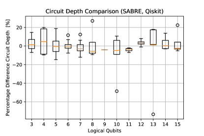
Figure 13: Box plots of the % difference comparison between Qiskit’s SABRE initial allocation method and the QUBO lowest SWAP allocation for circuit depth, over all applicable benchmark circuits. A negative value indicates that QUBO allocations had smaller depths.

Our analysis suggests that there is no universally best method among the ones considered. All the various initial allocation methods seem to do well for particular circuits, as shown by the wide and variable distributions in the plots. It would be of particular interest to know which features of circuit composition lead to the better performance of one allocation method versus another. We leave this to future work.

IV.2 QUBO performce for QUEKO Benchmarks

Recently, a set of known optimal-depth benchmark circuits were presented. In addition to proposing these QUEKO benchmarks, the authors also compared the performance of many different publically available compilers Tan and Cong (2020b). Their benchmarks are broken down into two main sets, one being B_NTF, or the ‘near-term feasible’ benchmarks, which range from optimal depth 5 to 45, and the other being B_SS, or the ‘scaling study’ benchmarks, ranging from optimal depth 100 to 900. Surprisingly, their results show that even the most competitive compilers available today have trouble getting close to the depth optimal solutions, deviating often to 5x the optimal depth or even greater (though t$\mid$ket$\rangle$ demonstrated remarkable performance, obtaining results very close to optimal). The benchmarks themselves are produced for a variety of hardware graphs, ranging from 16 qubits (Rigetti’s Aspen-4) to 53 qubits (Google’s Sycamore), so one can also look at the effect that increasing the space of possible allocations has on the compiler’s performance.

We were curious how QUBO initial allocations would do at finding the optimal allocation for these benchmarks, so we fed some QUBO initial allocations through t$\mid$ket$\rangle$ and Qiskit’s compiler to check which depths they could achieve. In this case, we are interested in how well the compiling process does as a whole and so we use the same optimization settings as Tan and Cong (2020b). After running the compilers we decompose any SWAP gates to CX (as well as BRIDGE for t$\mid$ket$\rangle$) and then record the realized depth. Again, we choose the lowest naive-SWAP QUBO allocation for each QUEKO benchmark circuit. An important point to note is that for these anneals, due to the larger size of some of the hardware, we only ran 100 samples of annealing in order to minimize runtime.

For most of the hardware used, we did not have access to their calibration data and therefore did not have any success probabilities to include in our QUBO coefficients. To work around this we removed the success probability term from Equation 14, and did a percent difference comparison for this form with and without the probability term using IBM-Melbourne calibration data and the benchmark set used in Subsection IV.1. We did this comparison to see if the quality of the allocations differed significantly between the forms. Unsurprisingly, the coefficent form that did not include success probability did worse at finding circuits with higher success probabilities, but in terms of SWAP counts the percent differences were scattered around 0, meaning both coefficient forms performed comparably.

In Figure 14 and Figure 15 we recreate figures 6 and 7 from Tan and Cong (2020b), but using QUBO initial allocations that are given to t$\mid$ket$\rangle$ and Qiskit’s compilers. It’s important to detail that we are using a different t$\mid$ket$\rangle$ and Qiskit version than is used in Tan and Cong (2020b), so the results are not directly comparable. This was discovered through some tests courtesy of the authors of Tan and Cong (2020b), where it was found that using the newer version of t$\mid$ket$\rangle$ results in significantly different compilation results Tan (2020). Therefore our results should be interpreted in the truest sense of how close we get to the optimal depths, and not compared directly to the results present in the QUEKO paper.

Plotted in Figure 14 is a comparison of Qiskit and t$\mid$ket$\rangle$’s compiled circuits on Aspen-4 and Sycamore for the B_NTF benchmark set. For Aspen-4, both compilers perform similarly given the same QUBO initial allocation, but diverge for the Sycamore circuits, where Qiskit clearly finds closer-to-optimal depths. It seems that the size difference of the hardware is the primary contributor to the difficulty of finding the depth-optimal allocations, and not the circuit depth. This same effect is seen in the B_SS benchmark set in Figure 15, where across an order of magnitude in circuit depth, we see very little variation as a function of depth, but a pronounced difference between the hardware being used. In particular, the smaller hardware sees close to optimal depths while the larger hardware is quite a bit from optimum. Comparing compilers, neither t$\mid$ket$\rangle$ nor Qiskit had particularly remarkable performance with the QUBO initial allocations, besides a small performance increase for t$\mid$ket$\rangle$ when moving to higher depth circuits initially.

An interesting experiment would be to see whether generating more samples during our anneal runs would combat the effect of the increase of the space of possible allocations as one moves to larger hardware and help in finding the more optimal allocations. Overall, it seems QUBO struggles with finding optimal depth allocations for larger hardwares and we leave it to future studies to see if some coefficient form or other change could improve on this performance.

(a) Aspen-4 (16 Qubits)

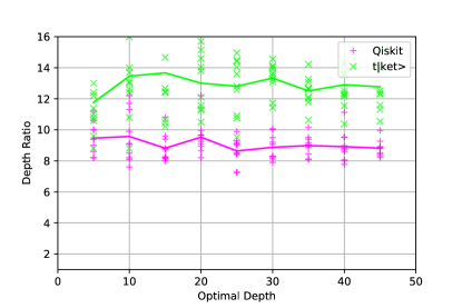
(b) Sycamore (53 Qubits)

Figure 14: Performance of a QUBO initial allocation given to t$\mid$ket$\rangle$ and Qiskit for the QUEKO B_NTF circuits (B_NTF = Benchmarks for near-term feasibility). Each data point is a unique circuit for a specific optimal depth, and lines are 10 circuits averages per depth per hardware-graph (180 circuits total).

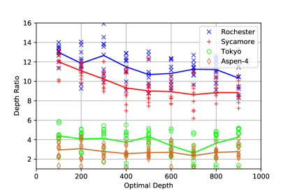
(a) t$\mid$ket$\rangle$ routing

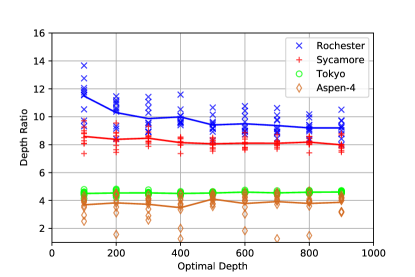
(b) Qiskit routing

Figure 15: Performance of a QUBO lowest naive-SWAP initial allocation given to t$\mid$ket$\rangle$ and Qiskit for the QUEKO B_ss circuits (B_ss = Benchmarks for Scaling Study). Each data point is a unique circuit for a specific optimal depth, and lines are 10 circuits averages per depth per hardware-graph (360 circuits total).

V Conclusion

The QUBO formulation has some very useful properties compared to other initial allocation methods. The coefficient form is very flexible, allowing the consideration of whatever metrics one cares to improve on for the allocation process. It is also agnostic to gate count — only limited on the solver end — therefore able to handle circuits of arbitrary depth (for both single and two-qubit gates). It is important to note that this method is specifically an initial allocation method, meaning it performs no further circuit optimization past finding good initial allocations.

While we showed that the QUBO method performs at the level of or slightly better than other available initial allocation methods, this just scratches the surface and many optimizations could be investigated. For example, one could attempt to improve the results by adjusting the simulated annealing hyperparameters. The results presented here use only the default settings provided in neal, but in general one could tweak the properties of the simulated annealer (e.g. temperature schedule, number of sweeps etc.) in order to produce better allocations. Furthermore, while we have not done so, it would be interesting to leverage special-purpose annealing hardware (whether classical or quantum) to see if we can obtain performance improvements, in particular for larger circuits with higher numbers of logical qubits. As mentioned in Subsection III.2, it would also be valuable to investigate a behind-the-scenes optimizer for the penalty coefficient values, as their magnitude did seem to effect allocation quality. In terms of future directions, it would be beneficial to know if generating more simulated annealing samples improves the quality of allocations when using larger hardware graphs (around the size of Sycamore, 53 qubits).

In general our results suggest that further research is necessary to learn the cause of the large variations seen in the performance of the initial allocation methods. Given the differences between circuits, it is likely that the circuit composition also plays a large role, most likely dominated by the two-qubit interactions and the necessary routing that must be done to satisfy connectivity constraints. Studying how the properties of a circuit affect the quality of allocation and routing methods will lead to even more improvements, and in particular for the QUEKO benchmarks will help close the optimality gap.

VI Acknowledgements

We thank Bochen Tan and Rodney Van Meter for helpful discussions. TRIUMF receives federal funding via a contribution agreement with the National Research Council of Canada. BD acknowledges funding from the TRIUMF student program, BioTalent Canada, and RBC Future Launch. We acknowledge the use of IBM Quantum services for this work to obtain hardware graphs and qubit calibration data. The views expressed are those of the authors, and do not reflect the official policy or position of IBM or the IBM Quantum team.

Appendix A Benchmark tables

This section contains the full set of data for the plots and benchmarks discussed in Section IV.

Table 2: Initial placement comparison of QUBO to the methods available in t$\mid$ket$\rangle$ using IBM Melbourne. Reported depths take into account all gates (not just CX). We bold the best performing method in each row (for ties, each tieing method is bolded).

		Initial		Line		Graph		QUBO
Circuit	n	Depth	CX count	Depth	CX	Depth	CX	Depth	CX
ex1_226	6	5	5	11	11	7	11	8	8
graycode6_47	6	5	5	5	5	5	5	5	5
xor5_254	6	5	5	11	11	7	11	8	8
ex-1_166	3	12	9	25	21	25	21	26	21
4mod5-v0_20	5	12	10	27	22	27	22	27	22
4mod5-v1_22	5	12	11	27	23	27	23	27	23
ham3_102	3	13	11	29	26	26	23	26	23
mod5d1_63	5	13	13	33	31	34	31	33	31
4gt11_83	5	16	14	32	32	31	26	31	26
rd32-v0_66	4	20	16	46	37	48	40	45	40
4mod5-v0_19	5	21	16	49	43	53	43	47	43
4mod5-v1_24	5	21	16	45	40	51	43	46	40
mod5mils_65	5	21	16	51	43	46	40	47	43
rd32-v1_68	4	21	16	47	37	49	40	47	40
alu-v0_27	5	21	17	46	44	46	44	40	38
3_17_13	3	22	17	47	38	47	38	47	38
alu-v1_29	5	22	17	47	44	47	44	44	38
alu-v2_33	5	22	17	39	38	39	38	49	44
4gt11_82	5	20	18	39	39	41	36	41	36
alu-v1_28	5	22	18	48	45	48	45	44	42
alu-v3_35	5	22	18	46	45	46	45	41	39
alu-v4_37	5	22	18	46	45	46	45	41	39
decod24-v2_43	4	30	22	73	58	73	58	72	58
miller_11	3	29	23	72	59	72	59	72	59
decod24-v0_38	4	30	23	64	53	73	59	73	59
alu-v3_34	5	30	24	71	63	75	66	69	60
mod5d2_64	5	32	25	90	73	71	67	89	73
4gt13_92	5	38	30	92	93	84	75	89	78
4gt13-v1_93	5	39	30	92	78	100	93	90	75
4mod5-v0_18	5	40	31	94	76	106	85	102	88
4mod5-bdd_287	7	41	31	116	97	102	88	90	82
decod24-bdd_294	6	40	32	104	92	106	92	91	77
one-two-three-v2_100	5	40	32	84	74	76	68	86	80
one-two-three-v3_101	5	40	32	97	89	95	80	94	83
4mod5-v1_23	5	41	32	108	92	104	83	104	89
rd32_270	5	47	36	119	93	118	105	117	99
4gt5_75	5	47	38	119	98	116	98	111	104
alu-bdd_288	7	48	38	122	110	116	119	112	101
alu-v0_26	5	49	38	112	104	115	107	112	98
decod24-v1_41	5	50	38	116	107	117	104	118	104
4gt5_76	5	56	46	130	118	137	127	125	112
4gt13_91	5	61	49	156	133	132	118	149	124
alu-v4_36	5	66	51	160	141	160	141	172	147
4gt13_90	5	65	53	173	155	142	128	159	134
4gt5_77	5	74	58	186	151	192	157	184	154
one-two-three-v1_99	5	76	59	189	179	207	191	199	173
rd53_138	8	56	60	205	174	169	162	136	162
decod24-v3_45	5	84	64	206	178	220	205	208	181
one-two-three-v0_98	5	82	65	211	179	217	200	213	206
4gt10-v1_81	5	84	66	213	186	211	195	214	186
aj-e11_165	5	86	69	189	177	217	189	213	186
4mod7-v0_94	5	92	72	238	228	228	204	227	201
alu-v2_32	5	92	72	227	201	222	204	235	195
4mod7-v1_96	5	94	72	226	198	228	195	235	195
mini_alu_305	10	69	77	237	242	249	239	241	251
mod10_176	5	101	78	256	216	270	240	246	216
4gt4-v0_80	6	101	79	231	223	243	229	251	229
4gt12-v0_88	6	108	86	267	242	288	269	273	245
qft_10	10	63	90	202	225	207	225	208	264
ising_model_10	10	70	90	172	156	70	90	70	90
sys6-v0_111	10	75	98	268	317	258	281	263	311
4_49_16	5	125	99	291	270	318	285	301	267
4gt12-v1_89	6	130	100	335	286	333	286	330	271
rd73_140	10	92	104	351	341	266	284	294	314
0410184_169	14	104	104	278	326	303	359	314	371
4gt4-v0_79	6	132	105	311	297	323	300	316	279
hwb4_49	5	134	107	332	302	346	293	364	314
mod10_171	5	139	108	351	297	356	309	336	294
4gt4-v0_78	6	137	109	322	310	338	322	290	292
4gt12-v0_87	6	131	112	338	331	333	313	302	298
4gt4-v0_72	6	137	113	363	338	372	335	350	320
4gt12-v0_86	6	135	116	353	350	337	320	309	305
4gt4-v1_74	6	154	119	393	347	399	356	407	356
ising_model_13	13	71	120	192	231	71	120	71	120
sym6_316	14	135	123	445	441	468	435	365	384
rd53_311	13	124	124	401	421	367	412	365	403
mini-alu_167	5	162	126	451	387	425	348	415	345
one-two-three-v0_97	5	163	128	428	380	440	371	403	356
rd53_135	7	159	134	409	389	432	425	374	389
sym9_146	12	127	148	491	496	401	424	439	451
ham7_104	7	185	149	490	446	508	473	423	425
decod24-enable_126	6	190	149	448	428	514	455	458	434
mod8-10_178	6	193	152	483	416	504	452	414	413
rd84_142	15	110	154	416	514	421	484	359	520
ex3_229	6	226	175	525	502	563	484	484	457
4gt4-v0_73	6	227	179	556	503	590	557	533	527
mod8-10_177	6	251	196	605	568	669	631	596	583
alu-v2_31	5	255	198	650	561	678	603	620	546
rd53_131	7	261	200	661	629	684	608	667	617
C17_204	7	253	205	614	586	693	658	641	595
alu-v2_30	6	285	223	815	790	770	787	746	649
mod5adder_127	6	302	239	773	716	841	869	767	728
rd53_133	7	327	256	839	796	919	991	905	769
majority_239	7	344	267	882	819	866	789	858	777
ex2_227	7	355	275	828	785	885	812	884	845
cm82a_208	8	337	283	878	796	876	820	782	775
sf_276	6	435	336	1200	1122	1270	1122	1125	924
sf_274	6	436	336	1081	978	1147	1047	1126	924
con1_216	9	508	415	1391	1327	1348	1324	1436	1351
wim_266	11	514	427	1341	1318	1553	1507	1445	1417
rd53_130	7	569	448	1544	1375	1480	1516	1535	1411
f2_232	8	668	525	1646	1593	1661	1572	1734	1599
cm152a_212	12	684	532	1831	1861	1637	1576	1529	1519
rd53_251	8	712	564	1778	1677	2012	1788	2049	1929
hwb5_53	6	758	598	2007	1720	2000	1786	1977	1825
cm42a_207	14	940	771	2523	2373	2450	2496	2559	2445
pm1_249	14	940	771	2523	2373	2450	2496	2637	2691
dc1_220	11	1038	833	2716	2576	2913	2936	2646	2552
squar5_261	13	1049	869	2962	2990	2818	2840	2945	2969
sqrt8_260	12	1659	1314	4377	4371	4579	4545	4477	4677
z4_268	11	1644	1343	4508	4490	4497	4427	4517	4481
radd_250	13	1781	1405	4764	4687	4805	4825	4914	4771
adr4_197	13	1839	1498	5011	5170	5069	5260	5031	5191
sym6_145	7	2187	1701	5690	5220	6047	5592	5638	5043
misex1_241	15	2676	2100	6803	7032	7078	7110	7126	7419
rd73_252	10	2867	2319	7732	7719	7839	7683	7669	7572
cycle10_2_110	12	3386	2648	9164	8924	9278	9377	9037	8861
hwb6_56	7	3736	2952	10128	9168	9706	8982	9980	9153
square_root_7	15	3847	3089	10712	11057	11065	11258	10923	10904
ham15_107	15	4819	3858	12989	13038	13214	13590	12668	12744
dc2_222	15	5242	4131	13988	14418	13800	14247	14255	14856
sqn_258	10	5458	4459	14739	15001	15703	15295	14940	14872
cm85a_209	14	6374	4986	16740	17703	16968	16359	16507	17358
rd84_253	12	7261	5960	19994	20480	19663	20633	19802	20705
root_255	13	8835	7493	24797	25871	24646	26831	24997	26153
co14_215	15	8570	7840	25916	30874	26640	31801	25802	30439
sym9_148	10	12087	9408	31530	32181	34459	37560	32345	30105
life_238	11	12511	9800	32916	33419	30051	31256	33315	33308
urf2_277	8	11390	10066	37298	39187	35895	37141	32922	33871
hwb7_59	8	13437	10681	36890	34777	35462	33697	34529	32590
max46_240	10	14257	11844	38559	38649	38196	38409	38757	39189
clip_206	14	17879	14772	48937	51783	51888	56595	48674	50853
9symml_195	11	19235	15232	51197	52288	52308	54592	52589	52399
sym9_193	11	19235	15232	51197	52288	52308	54592	50921	51703
dist_223	13	19694	16624	54200	57199	53746	56134	54059	57115
sao2_257	14	19563	16864	54667	59398	53269	58699	54269	59461
urf5_280	9	27822	23764	83215	83314	77664	79087	77885	79213
urf1_278	9	30955	26692	91184	92326	87149	90955	89282	92872
sym10_262	12	35572	28084	96157	97531	96637	111307	95346	96859
hwb8_113	9	38717	30372	102700	98604	105172	105819	109468	101511
urf2_152	8	44100	35210	120244	107762	124758	115100	115836	108608
plus63mod4096_163	13	72246	56329	201604	200857	189834	195673	189141	193045
urf3_279	10	70702	60380	202696	212168	201968	211580	201791	208862
urf5_158	9	89145	71932	240381	232375	239424	225166	243031	228574
urf6_160	15	93645	75180	255359	267393	254680	267012	254871	266559
urf1_149	9	99585	80878	276750	261598	276528	261598	274654	259522
plus63mod8192_164	14	105142	81865	278241	288745	276074	286609	275721	286279
hwb9_119	10	116199	90955	306090	297445	306286	297292	307302	298546
ground_state_estimation_10	13	245614	154209	465677	460929	401363	354942	423376	390003
urf3_155	10	229365	185276	647997	633602	627662	600530	631267	603608
urf4_187	11	264330	224028	690886	700740	741405	765486	698447	726072

Table 3: Initial placement comparison of QUBO to the methods available in Qiskit, using IBM Melbourne. Reported depths take into account all gates (not just CX). We bold the best performing method in each row (for ties, each tieing method is bolded).

		Initial		Trivial		Dense		Noise		SABRE		QUBO
Circuit	n	Depth	CX count	Depth	CX	Depth	CX	Depth	CX	Depth	CX	Depth	CX
ex1_226	6	5	5	30	47	23	32	12	17	8	11	8	11
graycode6_47	6	5	5	5	5	12	14	13	20	5	11	5	5
xor5_254	6	5	5	30	47	23	32	12	17	8	11	8	11
ex-1_166	3	12	9	29	24	27	24	28	24	29	24	27	24
4mod5-v0_20	5	12	10	39	43	27	25	30	31	21	22	21	19
4mod5-v1_22	5	12	11	36	35	21	20	33	32	24	26	21	20
ham3_102	3	13	11	27	23	25	23	27	23	22	20	23	20
mod5d1_63	5	13	13	45	52	35	37	53	52	33	37	36	37
4gt11_83	5	16	14	36	32	33	32	38	35	28	29	25	23
rd32-v0_66	4	20	16	47	43	49	43	44	40	39	37	46	40
4mod5-v0_19	5	21	16	53	55	51	46	56	52	47	43	45	43
4mod5-v1_24	5	21	16	54	52	48	46	54	49	50	49	43	37
mod5mils_65	5	21	16	59	61	53	52	58	52	48	40	41	40
rd32-v1_68	4	21	16	48	43	50	43	46	40	40	37	48	40
alu-v0_27	5	21	17	61	59	58	50	56	50	44	41	52	50
3_17_13	3	22	17	53	44	49	44	47	38	41	38	47	38
alu-v1_29	5	22	17	52	50	56	47	51	44	43	38	47	41
alu-v2_33	5	22	17	50	44	53	47	53	50	40	35	44	41
4gt11_82	5	20	18	52	48	43	42	56	54	38	39	37	39
alu-v1_28	5	22	18	52	48	59	54	60	54	52	51	52	51
alu-v3_35	5	22	18	65	60	64	54	59	54	50	45	57	54
alu-v4_37	5	22	18	65	63	62	54	59	54	48	45	57	54
decod24-v2_43	4	30	22	68	58	69	58	65	55	71	64	65	55
miller_11	3	29	23	71	62	75	62	71	62	72	62	71	62
decod24-v0_38	4	30	23	73	65	74	65	67	59	73	65	66	59
alu-v3_34	5	30	24	76	66	78	66	78	66	77	69	76	69
mod5d2_64	5	32	25	93	88	88	82	93	88	83	82	80	70
4gt13_92	5	38	30	115	102	112	99	106	90	95	84	90	90
4gt13-v1_93	5	39	30	106	90	97	87	91	75	85	69	86	81
4mod5-v0_18	5	40	31	101	100	100	91	99	82	90	82	105	94
4mod5-bdd_287	7	41	31	109	118	105	100	115	118	103	100	98	94
decod24-bdd_294	6	40	32	86	77	103	95	95	92	100	104	98	95
one-two-three-v2_100	5	40	32	116	107	106	95	98	89	98	95	102	98
one-two-three-v3_101	5	40	32	106	98	102	95	113	101	94	83	93	83
4mod5-v1_23	5	41	32	106	104	107	98	103	95	95	89	99	89
rd32_270	5	47	36	119	123	105	96	124	123	117	114	108	102
4gt5_75	5	47	38	120	110	135	119	107	98	106	98	112	101
alu-bdd_288	7	48	38	167	167	131	131	117	107	119	110	115	110
alu-v0_26	5	49	38	149	134	132	110	145	128	106	98	112	98
decod24-v1_41	5	50	38	137	116	125	110	114	101	130	119	114	104
4gt5_76	5	56	46	148	139	127	115	141	127	132	124	120	112
4gt13_91	5	61	49	158	142	143	124	135	118	140	127	145	136
alu-v4_36	5	66	51	171	147	156	141	157	132	160	147	169	150
4gt13_90	5	65	53	174	158	153	134	145	128	150	137	161	152
4gt5_77	5	74	58	205	184	198	184	200	178	195	172	185	172
one-two-three-v1_99	5	76	59	191	182	187	170	187	170	186	182	179	164
rd53_138	8	56	60	176	225	190	189	177	195	148	177	188	174
decod24-v3_45	5	84	64	248	211	221	193	216	187	212	187	196	181
one-two-three-v0_98	5	82	65	226	206	199	176	212	185	199	176	206	182
4gt10-v1_81	5	84	66	225	201	195	174	207	183	213	183	200	180
aj-e11_165	5	86	69	258	228	215	195	226	195	228	207	212	189
4mod7-v0_94	5	92	72	269	228	228	216	230	195	234	201	230	207
alu-v2_32	5	92	72	259	231	228	213	249	216	247	225	246	231
4mod7-v1_96	5	94	72	248	225	234	219	242	216	236	219	218	189
mini_alu_305	10	69	77	233	275	211	245	256	248	216	245	234	260
mod10_176	5	101	78	284	246	269	231	260	222	256	222	256	228
4gt4-v0_80	6	101	79	289	283	298	277	267	241	263	241	244	235
4gt12-v0_88	6	108	86	311	305	310	281	305	281	266	245	257	239
qft_10	10	63	90	283	588	238	339	185	288	226	360	250	336
ising_model_10	10	70	90	267	327	178	153	132	129	136	123	70	90
sys6-v0_111	10	75	98	308	410	329	341	297	311	284	320	259	305
4_49_16	5	125	99	350	306	316	270	323	285	334	309	333	288
4gt12-v1_89	6	130	100	408	379	376	349	359	343	339	310	338	319
rd73_140	10	92	104	324	434	314	344	349	374	333	362	303	332
0410184_169	14	104	104	295	413	308	428	335	389	333	440	324	395
4gt4-v0_79	6	132	105	375	321	342	315	353	306	332	282	326	297
hwb4_49	5	134	107	367	314	348	299	325	287	338	305	351	302
mod10_171	5	139	108	406	363	378	327	335	294	319	294	332	306
4gt4-v0_78	6	137	109	392	340	350	322	369	325	349	313	343	316
4gt12-v0_87	6	131	112	378	337	363	331	363	352	356	331	354	328
4gt4-v0_72	6	137	113	400	395	382	335	367	356	344	347	384	338
4gt12-v0_86	6	135	116	394	353	376	344	379	368	358	347	367	344
4gt4-v1_74	6	154	119	434	407	390	344	400	386	401	380	417	368
ising_model_13	13	71	120	267	357	317	273	229	264	267	321	71	120
sym6_316	14	135	123	440	453	389	423	373	393	386	399	439	438
rd53_311	13	124	124	433	472	354	439	402	463	364	430	429	436
mini-alu_167	5	162	126	497	438	446	387	438	381	432	375	380	351
one-two-three-v0_97	5	163	128	483	428	423	371	402	353	421	365	413	377
rd53_135	7	159	134	464	485	436	422	413	398	441	398	422	425
sym9_146	12	127	148	494	568	434	520	470	583	423	478	457	523
ham7_104	7	185	149	560	506	502	446	455	407	524	491	461	428
decod24-enable_126	6	190	149	554	518	507	449	464	428	507	467	510	449
mod8-10_178	6	193	152	610	563	565	512	518	485	452	422	483	437
rd84_142	15	110	154	405	580	464	634	452	547	348	502	426	607
ex3_229	6	226	175	690	631	620	547	588	529	573	553	581	514
4gt4-v0_73	6	227	179	654	596	607	545	653	587	597	533	552	497
mod8-10_177	6	251	196	737	712	666	607	680	622	615	568	641	592
alu-v2_31	5	255	198	739	627	664	576	704	636	612	555	647	564
rd53_131	7	261	200	717	647	682	620	679	614	638	587	717	623
C17_204	7	253	205	774	748	632	595	712	664	676	679	659	613
alu-v2_30	6	285	223	839	772	759	685	719	664	778	703	731	673
mod5adder_127	6	302	239	886	806	786	710	824	761	773	689	772	701
rd53_133	7	327	256	911	814	786	751	855	805	885	787	779	739
majority_239	7	344	267	1009	909	920	816	949	828	947	852	890	795
ex2_227	7	355	275	1103	1013	921	821	930	842	896	836	952	881
cm82a_208	8	337	283	1019	1102	917	874	935	871	981	922	909	841
sf_276	6	435	336	1259	1131	1183	1080	1184	1044	1108	990	1079	996
sf_274	6	436	336	1271	1143	1178	1068	1197	1029	1124	1017	1039	939
con1_216	9	508	415	1602	1540	1339	1276	1432	1333	1421	1369	1364	1327
wim_266	11	514	427	1373	1330	1433	1339	1461	1405	1534	1405	1428	1324
rd53_130	7	569	448	1743	1582	1523	1420	1471	1339	1496	1360	1496	1372
f2_232	8	668	525	1970	1884	1642	1509	1746	1617	1782	1611	1717	1536
cm152a_212	12	684	532	1837	1672	1954	1795	1825	1639	1823	1747	1881	1681
rd53_251	8	712	564	2294	2166	1952	1743	1853	1728	2035	1848	1847	1668
hwb5_53	6	758	598	2278	2059	2047	1816	1979	1792	1906	1822	1941	1801
cm42a_207	14	940	771	2660	2535	2482	2334	2531	2325	2728	2583	2825	2763
pm1_249	14	940	771	2660	2535	2482	2334	2531	2325	2728	2583	2645	2517
dc1_220	11	1038	833	3082	2996	2886	2669	2956	2744	2995	2789	2896	2759
squar5_261	13	1049	869	3122	3047	3258	3167	3171	3173	2730	2708	3205	3002
sqrt8_260	12	1659	1314	5095	4860	4742	4572	4765	4488	4769	4521	4927	4557
z4_268	11	1644	1343	5007	4847	4657	4382	4705	4475	4753	4553	4657	4367
radd_250	13	1781	1405	5178	4930	5395	5134	5095	4678	5004	4657	5101	4846
adr4_197	13	1839	1498	5303	5182	5116	4876	5373	5110	5269	5026	5342	5224
sym6_145	7	2187	1701	6647	6105	5675	5271	5724	5160	5656	5133	5748	5091
misex1_241	15	2676	2100	7978	7407	7881	7455	7853	7422	7534	6948	7150	6846
rd73_252	10	2867	2319	9092	8823	8148	7623	7921	7581	8090	7752	8043	7434
cycle10_2_110	12	3386	2648	10252	9776	10002	9323	9542	8759	9507	8765	9410	8702
hwb6_56	7	3736	2952	11617	10761	10182	9117	9969	9054	9551	8844	9694	9009
square_root_7	15	3847	3089	14605	15506	14905	15938	14703	16283	14777	15659	14434	15251
ham15_107	15	4819	3858	15092	14514	14598	14073	13566	12915	14058	13347	14653	14067
dc2_222	15	5242	4131	14889	14430	15323	14649	14418	13755	15569	14625	15063	14148

References

- Siraichi et al. (2018) M. Y. Siraichi, V. F. d. Santos, S. Collange, and F. M. Q. Pereira, in Proceedings of the 2018 International Symposium on Code Generation and Optimization, CGO 2018 (Association for Computing Machinery, New York, NY, USA, 2018) p. 113–125.
- Tan and Cong (2020a) B. Tan and J. Cong, “Optimal layout synthesis for quantum computing,” (2020a), arXiv:2007.15671 [cs.AR] .
- Dueck et al. (2018) G. W. Dueck, A. Pathak, M. M. Rahman, A. Shukla, and A. Banerjee, in 2018 21st Euromicro Conference on Digital System Design (DSD) (2018) pp. 680–684.
- Li et al. (2020) S. Li, X. Zhou, and Y. Feng, “Qubit mapping based on subgraph isomorphism and filtered depth-limited search,” (2020), arXiv:2004.07138 [quant-ph] .
- Ghosh et al. (2020) M. Ghosh, N. Dey, D. Mitra, and A. Chakrabarti, Advances in Intelligent Systems and Computing 996, 127 (2020).
- Deng et al. (2020) H. Deng, Y. Zhang, and Q. Li, “Codar: A contextual duration-aware qubit mapping for various nisq devices,” (2020), arXiv:2002.10915 [quant-ph] .
- Zhang et al. (2020) C. Zhang, Y. Chen, Y. Jin, W. Ahn, Y. Zhang, and E. Z. Zhang, “A depth-aware swap insertion scheme for the qubit mapping problem,” (2020), arXiv:2002.07289 [cs.ET] .
- Childs et al. (2019) A. M. Childs, E. Schoute, and C. M. Unsal, Proceedings of TQC 2019, LIPIcs 135 (2019), https://doi.org/10.4230/LIPIcs.TQC.2019.3.
- Zulehner and Wille (2019) A. Zulehner and R. Wille, in Proceedings of the 24th Asia and South Pacific Design Automation Conference, ASPDAC ’19 (Association for Computing Machinery, New York, NY, USA, 2019) p. 185–190.
- Brierley (2015) S. Brierley, “Efficient implementation of quantum circuits with limited qubit interactions,” (2015), arXiv:1507.04263 [quant-ph] .
- Paler (2019) A. Paler, in Quantum Technology and Optimization Problems, edited by S. y. Feld and C. Linnhoff-Popien (Springer International Publishing, Cham, 2019) pp. 207–217, 1811.08985 .
- Paler et al. (2020) A. Paler, L. M. Sasu, A. Florea, and R. Andonie, “Machine learning optimization of quantum circuit layouts,” (2020), arXiv:2007.14608 [quant-ph] .
- Nash et al. (2020) B. Nash, V. Gheorghiu, and M. Mosca, Quantum Science and Technology 5, 025010 (2020).
- Lin et al. (2019) J. X. Lin, E. R. Anschuetz, and A. W. Harrow, “Using spectral graph theory to map qubits onto connectivity-limited devices,” (2019), arXiv:1910.11489 [quant-ph] .
- Smith et al. (2020a) K. Smith, M. Thornton, M. Soeken, B. Schmitt, and G. de Micheli, Electronic Proceedings in Theoretical Computer Science, EPTCS 318, 106 (2020a), arXiv:1901.02406 .
- Webber et al. (2020) M. Webber, S. Herbert, S. Weidt, and W. K. Hensinger, “Efficient qubit routing for a globally connected trapped ion quantum computer,” (2020), arXiv:2002.12782 [quant-ph] .
- Amy and Gheorghiu (2020) M. Amy and V. Gheorghiu, Quantum Science and Technology 5, 034016 (2020).
- Smith et al. (2020b) R. S. Smith, E. C. Peterson, M. G. Skilbeck, and E. J. Davis, Quantum Science and Technology 5, 044001 (2020b).
- Sivarajah et al. (2020) S. Sivarajah, S. Dilkes, A. Cowtan, W. Simmons, A. Edgington, and R. Duncan, Quantum Science and Technology (2020).
- et al. (2019) H. A. et al., “Qiskit: An open-source framework for quantum computing,” (2019).
- Google (2019) Google, “Cirq,” https://github.com/quantumlib/Cirq.git (2019).
- Wille et al. (2019) R. Wille, L. Burgholzer, and A. Zulehner, in Proceedings - Design Automation Conference (2019) arXiv:1907.02026 .
- Li et al. (2019) G. Li, Y. Ding, and Y. Xie, in Proceedings of the Twenty-Fourth International Conference on Architectural Support for Programming Languages and Operating Systems, ASPLOS ’19 (Association for Computing Machinery, New York, NY, USA, 2019) p. 1001–1014.
- Cowtan et al. (2019) A. Cowtan, S. Dilkes, R. Duncan, A. Krajenbrink, W. Simmons, and S. Sivarajah, in 14th Conference on the Theory of Quantum Computation, Communication and Cryptography (TQC 2019), Leibniz International Proceedings in Informatics (LIPIcs), Vol. 135, edited by W. van Dam and L. Mancinska (Schloss Dagstuhl–Leibniz-Zentrum fuer Informatik, Dagstuhl, Germany, 2019) pp. 5:1–5:32.
- Pedram and Shafaei (2016) M. Pedram and A. Shafaei, IEEE Circuits and Systems Magazine 16, 62 (2016).
- Herbert and Sengupta (2018) S. Herbert and A. Sengupta, “Using reinforcement learning to find efficient qubit routing policies for deployment in near-term quantum computers,” (2018), arXiv:1812.11619 [quant-ph] .
- Pozzi et al. (2020) M. G. Pozzi, S. J. Herbert, A. Sengupta, and R. D. Mullins, “Using reinforcement learning to perform qubit routing in quantum compilers,” (2020), arXiv:2007.15957 [quant-ph] .
- Murali et al. (2019) P. Murali, J. M. Baker, A. J. Abhari, F. T. Chong, and M. Martonosi, International Conference on Architectural Support for Programming Languages and Operating Systems - ASPLOS , 1015 (2019), arXiv:1901.11054 .
- Wilson et al. (2020) E. Wilson, S. Singh, and F. Mueller, “Just-in-time quantum circuit transpilation reduces noise,” (2020), arXiv:2005.12820 [quant-ph] .
- P. Jurcevic et al. (2020) P. Jurcevic et al., “Demonstration of quantum volume 64 on a superconducting quantum computing system,” (2020), arXiv:2008.08571 [quant-ph] .
- Nishio et al. (2020) S. Nishio, Y. Pan, T. Satoh, H. Amano, and R. V. Meter, ACM Journal on Emerging Technologies in Computing Systems 16, 1–25 (2020).
- Tannu and Qureshi (2018) S. S. Tannu and M. K. Qureshi, “A case for variability-aware policies for nisq-era quantum computers,” (2018), arXiv:1805.10224 [quant-ph] .
- Bhattacharjee et al. (2019) D. Bhattacharjee, A. A. Saki, M. Alam, A. Chattopadhyay, and S. Ghosh, “Muqut: Multi-constraint quantum circuit mapping on noisy intermediate-scale quantum computers,” (2019), arXiv:1911.08559 [quant-ph] .
- Finigan et al. (2018) W. Finigan, M. Cubeddu, T. Lively, J. Flick, and P. Narang, “Qubit allocation for noisy intermediate-scale quantum computers,” (2018), arXiv:1810.08291 [quant-ph] .
- Zhou et al. (2020) X. Zhou, S. Li, and Y. Feng, IEEE Transactions on Computer-Aided Design of Integrated Circuits and Systems , 1 (2020), 1908.08853 .
- (36) https://github.com/bdury/QUBO-for-Qubit-Allocation.
- Tan and Cong (2020b) B. Tan and J. Cong, IEEE Transactions on Computers , 1–1 (2020b).
- Kochenberger et al. (2014) G. Kochenberger, J. K. Hao, F. Glover, M. Lewis, Z. Lü, H. Wang, and Y. Wang, Journal of Combinatorial Optimization 28, 58 (2014).
- Glover et al. (2018) F. Glover, G. Kochenberger, and Y. Du, “A tutorial on formulating and using qubo models,” (2018), arXiv:1811.11538 [cs.DS] .
- Lucas (2014) A. Lucas, Frontiers in Physics 2 (2014), 10.3389/fphy.2014.00005.
- Lodewijks (2019) B. Lodewijks, “Mapping np-hard and np-complete optimisation problems to quadratic unconstrained binary optimisation problems,” (2019), arXiv:1911.08043 [cs.DS] .
- Burkard (2013) R. E. Burkard, in Handbook of Combinatorial Optimization, Vol. 5-5 (Springer New York, 2013) pp. 2741–2814.
- D-Wave Systems Inc. (2020) D-Wave Systems Inc., “neal,” https://github.com/dwavesystems/dwave-neal (2020).
- Zulehner et al. (2018) A. Zulehner, A. Paler, and R. Wille, in 2018 Design, Automation Test in Europe Conference Exhibition (DATE) (2018) pp. 1135–1138.
- Tan (2020) B. Tan, “Personal Communication,” (2020).