Nearest-Neighbor Functions for Disordered Stealthy Hyperuniform Many-Particle Systems

Abstract

Disordered stealthy many-particle systems in $d$-dimensional Euclidean space $\mathbb{R}^{d}$ are exotic amorphous states of matter that suppress any single scattering events for a finite range of wavenumbers around the origin in reciprocal space. They are currently the subject of intense fundamental and practical interest. We derive analytical formulas for the nearest-neighbor functions of disordered stealthy many-particle systems. First, we analyze asymptotic small-$r$ approximations and expansions of the nearest-neighbor functions based on the pseudo-hard-sphere ansatz. We then consider the problem of determining how many of the standard $n$-point correlation functions are needed to determine the nearest neighbor functions, and find that a finite number suffice. Via theoretical and computational methods, we are able to compare the large-$r$ behavior of these functions for disordered stealthy systems to those belonging to crystalline lattices. Such ordered and disordered stealthy systems have bounded hole sizes, and thus compact support for their nearest-neighbor functions. However, we find that the approach to the critical-hole size can be quantitatively different, emphasizing the importance of hole statistics in distinguishing ordered and disordered stealthy configurations. We argue that the probability of finding a hole close to the critical-hole size should decrease as a power law with an exponent only dependent on the space dimension $d$ for ordered systems, but that this probability decays asymptotically faster for disordered systems, with either an increase in the exponent of the power law or a crossover into a decay faster than any power law. This implies that holes close to the critical-hole size are rarer in disordered systems. The rarity of observing large holes in disordered systems creates substantial numerical difficulties in sampling the nearest neighbor distributions near the critical-hole size. This motivates both the need for new computational methods for efficient sampling and the development of novel theoretical methods for ascertaining the behavior of holes close to the critical-hole size. We also devise a simple analytical formula that accurately describes these systems in the underconstrained regime for all $r$. These results provide a theoretical foundation for the analytical description of the nearest-neighbor functions of stealthy systems in the disordered, underconstrained regime, and can serve as a basis for analytical theories of material and transport properties of these systems.

Keywords: nearest-neighbor functions, stealthy hyperuniformity, bounded hole size, point processes

1 Introduction

In the study of disordered many-body systems, a large body of recent work (see Ref. [1] and references therein) has promoted the concept of hyperuniformity [2] as a useful principle for identifying exotic disordered systems with novel physical properties [1, 3, 4, 1, 6, 7, 8, 9, 10, 11, 12, 13, 14, 15]. Hyperuniformity refers to systems with an anomalous suppression of long-range density fluctuations. More specifically, given a $d$-dimensional point process, one considers the variance $\sigma^{2}_{N}(R)$ of the number of particles within a spherical window of radius $R$ as one uniformly varies the location of the window or averages over an enemble. Quantitatively, a hyperuniform system is one in which [2]

$$\lim_{R\to\infty}\frac{\sigma^{2}_{N}(R)}{v_{1}(R)}=0,$$ (1)

where $v_{1}(R)=\pi^{d/2}R^{d}/\Gamma(1+d/2)$ is the volume of a $d$-dimensional sphere of radius $R$. For typical disordered systems, $\sigma_{N}^{2}(R)$ grows as $R^{d}$, so the above ratio tends to a positive constant. Thus, hyperuniformity is defined by an asympotically slow growth of the number variance, which is a key measure of the density fluctuations associated to a given scale in the system. Equivalently, one can also identify hyperuniformity through the following condition on the structure factor $S({\bi k})$ (obtainable through the scattering intensity) associated with the point process [2]:

$$\lim_{|{\bi k}|\to 0}S({\bi k})=0.$$ (2)

Note that this definition excludes the forward scattering contribution in the scattering pattern. The structure factor is related to the widely-used total correlation function $h({\bi r})=g_{2}({\bi r})-1$, where $g_{2}({\bi r})$ is the pair correlation function, through a Fourier transform [16]:

$$S({\bi k})=1+\rho\int_{\mathbb{R}^{d}}e^{-i{\bi k}\cdot{\bi r}}h({\bi r})\,\rmd{\bi r}.$$ (3)

Thus, Eq. (2) amounts to the following sum rule on the two-point statistics of the point process [1]:

$$\int_{\mathbb{R}^{d}}h({\bi r})\,\rmd{\bi r}=-1.$$ (4)

There are many examples of hyperuniform systems, both ordered and disordered. In the ordered case, we have trivially that all perfect crystals are hyperuniform, due to the presence of a Bragg-peak spectrum. As a less trivial ordered example, we have that perfect quasicrystals are also hyperuniform [17, 18, 19]. Disordered hyperuniform systems are considerably more exotic, since typical disordered systems such as liquids and gases have $S(k\to 0)\neq 0$ [2]. Examples include avian photoreceptor patterns [20], perfect glasses [3], maximally random jammed packings [21, 22, 23, 24, 25, 26], density fluctuations in the large-scale structure of the Universe [27, 28, 29, 30], fermionic point processes [31, 32], and superfluid helium [33, 34].

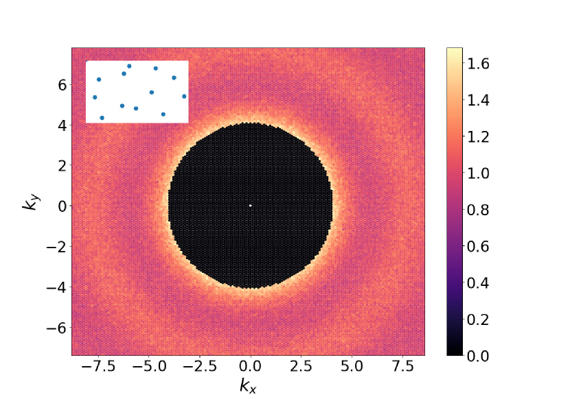
(a)

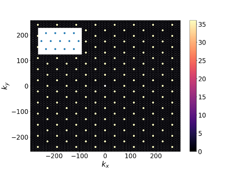
(b)

Figure 1: Scattering patterns (structure factor) for two 2D stealthy hyperuniform point processes and small corresponding representative samples of the underlying real-space point processes (inset). (a) The scattering pattern of a triangular lattice (see inset). (b) The scattering pattern of a disordered stealthy hyperuniform system (see inset). Excluding the forward scattering contribution, both structure factors exhibit the signature exclusion region around the origin in which there are no single-scattering events, implying a suppression of density fluctuations from infinite down to finite wavelengths. However, the disordered pattern lacks sharp Bragg peaks, with the diffuse behavior of the scattering pattern away from the origin being closer to that of a liquid. Note that while the stealthy disordered pattern possesses short-range order more typical of a disordered liquid or gas (see inset), it has a bounded hole size [1, 2].

In this article, we will focus on an important subset of hyperuniformity known as stealthy hyperuniformity [4]. Stealthy hyperuniformity further generalizes the notion of mimicking an aspect of a crystal’s long wavelength behavior while maintaining local disorder. A stealthy hyperuniform system is one in which the structure factor vanishes in an entire range of wavelengths near the origin [4]:

$$S({\bi k})=0,\quad 0<|{\bi k}|<K.$$ (5)

Crystals, due to their Bragg peaks, trivially satisfy this condition. Interestingly, one can also find disordered systems that obey stealthy hyperuniformity [36, 5, 12]. An example of the scattering pattern for a stealthy disordered system is compared to a stealthy ordered system in Fig. 1. While both the ordered crystal and the disordered pattern exhibit a spherical exclusion region with no scattering, the disordered pattern exhibits the continuous scattering usually associated with liquids and gases everywhere else in the domain [1, 5].

One of the most powerful techniques for studying stealthy hyperuniform systems is a collective coordinate optimization procedure [38, 36, 39, 4, 14, 15, 40, 5, 6, 42] that involves finding the ground states of a class of bounded pair potentials with compact support in Fourier space [38, 36, 40, 4, 5]. The highly degenerate ground states of such potentials are stealthy hyperuniform by construction. This technique suggests the utility of defining a control parameter $\chi$, which is a dimensionless measure of the ratio of constrained degrees of freedom to the total degrees of freedom in such an optimization procedure. In the thermodynamic limit, this control parameter can be written [4, 5]

$$\chi=\frac{v_{1}(K)}{2\rho d(2\pi)^{d}},$$ (6)

where $\rho$ is the number density of the point process. Since this formula involves only the general properties of a stealthy system, such as the cutoff wavevector $K$, it can be used to classify stealthy systems even beyond the collective coordinate framework. A system with a small $\chi$ (relatively unconstrained) is disordered, and as $\chi$ increases, the short-range order increases within a disordered regime [38, 36, 39, 4, 14, 15, 40, 5, 6, 42]. Upon reaching a critical value of $\chi$, there is a phase transition to predominantly crystalline ground states [38, 36, 39, 4, 14, 15, 40, 5, 6, 42].

While the stealthiness of crystals is a trivial outcome of Bragg scattering, disordered stealthy systems display highly unusual statistical geometric properties. For example, all stealthy hyperuniform systems have a bounded hole size [1, 2], meaning that one cannot find a sphere devoid of particles above a certan radius, and an “anti-concentration” property that strictly bounds the density from above in a large enough subset of the system [2]. As a result of these crystal-like geometric properties and fluid-like short-range order, the disordered variants exhibit novel physical properties with implications for materials discovery. In particular, the isotropy of these disordered phases generates direction-independent physical properties, in stark contrast to typical crystalline systems. For example, disordered stealthy point processes, which can be mapped to cellular dielectric networks, led to the first discovery of a complete isotropic photonic band gap [6, 9, 7, 8, 10, 11], which enables the construction of free-form waveguides [11, 8, 9]. In addition, they possess certain nearly optimal transport properties (while remaining isotropic) when used to model both inclusion-based and cellular composites [12, 13], which emphasizes the importance of the underlying point process geometry. The link between the unique structural properties of stealthy disordered processes and their obvious utility for materials design is still not fully understood, but it has been conjectured that the bounded hole size property plays a key role in producing their novel thermodynamic and physical properties, including their desirable band gap, optical, and transport behaviors [1].

However, there is still much we do not know about the fundamental structural properties of disordered stealthy processes. One such type of fundamental question involves determining the analytical functional forms for the nearest-neighbor functions of a given particle or void point in the system [43, 3]. These functions encode the statistical distribution of intuitive geometric concepts such as the size of holes in a system, making them good candidates for capturing the statistical properties of stealthy disordered processes, which possess bounded hole sizes. These functions come in two general varieties: the void nearest-neighbor functions, which identifies the nearest neighbor of an arbitrary spatial point in the system, and the particle nearest-neighbor functions, which identify the nearest neighbor of an arbitrary particle in the system. While these varieties are generally distinct, they can sometimes be related to each other for specific point processes, such as equilibrium hard spheres [43, 3].

The nearest-neighbor functions and variants have played a key role in investigating problems in a variety of scientific fields. These include the application of the Wigner surmise in nuclear physics [45, 31], their fundamental appearance in the theory of liquids and other amorphous systems [46, 47, 43, 3, 48, 49, 50, 51, 52, 53, 54, 55, 56, 57, 58, 59, 60], the study of astrophysical dynamics [61], the characterization of membranes in cells [62], and the modeling of granular flows [63]. They have also been applied to the study of fundamental problems in the mathematical discipline of discrete geometry, including the covering and quantizer problems [64].

In addition to their utility in describing systems of fundamental scientific and mathematical interest, one can use them to derive statistics to characterize the microstructure of complex materials. One example of such a derived quantity is the distribution of pore sizes in a heterogeneous material [65, 66]. They can also be used to estimate transport properties, such as the rate of a diffusion-controlled reaction [67, 68, 69, 65]. Determining accurate formulas for the nearest-neighbor functions of a system can thus aid in materials discovery.

Based on strong theoretical and computational evidence, Zhang, Stillinger, and Torquato [1] formulated the surprising conjecture that any stealthy system has the aforementioned bounded hole size property, which was subsequently proven by Ghosh and Lebowitz [2]. It is important to note that the converse is not true; there exist systems such as random sequential addition at the saturation state that have bounded holes by construction but are not stealthy [70, 71]. The nearest-neighbor functions of disordered stealthy systems have also been studied computationally in light of their connection with transport properties [12], and a few results are known based on analytical approximations we will use later in this article [5]. However, to date, there has not been a systematic theoretical investigation of their nearest-neighbor statistics, and little is known about their asymptotics as the critical-hole radius (i.e. radius of the largest possible hole) $r_{c}$ is approached.

In this article, we obtain accurate theoretical expressions for these functions for disordered stealthy hyperuniformity. The accuracy of our formulas is verified through simulations presented in Refs. [4, 5, 6, 42, 1]. We pay particular attention to the small-$r$ behavior of the functions and asymptotics on approach to the critical-hole size.

In the small-$r$ regime, we are able to obtain a variety of approximations and bounds due to the pseudo-hard-sphere ansatz [5], which is valid when considering stealthy point processes with low to intermediate $\chi$. In particular, we are able to derive small-$r$ expansions that can provide useful approximations, even outside the small-$\chi$ limit. We also provide supporting evidence for a new conjecture on the validity of two upper bounds. Going beyond the methods based on the pseudo-hard-sphere ansatz, we demonstrate that the nearest-neighbor functions can be determined by a finite number of $g_{n}({\bi r}^{n})$, in contrast with the general case, which requires an infinite number of $g_{n}({\bi r}^{n})$. In the large-$r$ regime, we consider the scaling behavior of these functions as they approach the critical-hole size. We compare their behavior to that of ordered point configurations through theoretical arguments and the analysis of simulation data. We encounter substantial numerical difficulty due to the rarity of finding holes close to the critical-hole radius, which we argue is exacerbated in disordered systems due to the expectation that the hole probability vanishes more quickly in the presence of disorder. This difficulty points to the need for the development of more efficient simulation methods for these exotic potentials as well as further research into theoretical methods for determining the behavior of holes near the critical-hole radius. We also discuss a useful prescription for linking the small-$r$ and near-$r_{c}$ regime into an approximation accurate over all $r$, as validated by comparison to simulations. Finally, we comment on the large-$r$ asymptotic behavior of the nearest-neighbor functions of stealthy systems at positive temperature, where they lose their strict stealthiness property, and show that they are also expected to lose their bounded holes property.

Section 2 covers the basic theory of the nearest-neighbor functions and stealthy hyperuniform point processes. In Sec. 3, we provide analytical bounds and approximations obtained through the pseudo-hard-sphere approximation valid at small-$r$. We consider the problem of determining how many of the $g_{n}({\bi r}^{n})$ are needed to determine the nearest-neighbor functions of stealthy systems in Section 4. Section 5 presents a description of the asymptotic behavior near the critical-hole size of the nearest-neighbor functions. Section 6 discusses the problem of linking the small and large-$r$ regimes to obtain expressions for the nearest-neighbor functions over all $r$. Section 7 describes positive temperature results. In Sec. 8, we summarize our findings and makes some concluding remarks.

2 Preliminaries

2.1 Definitions for Nearest-Neighbor Functions

2.1.1 “Void” Quantities

The nearest-neighbor functions are special cases of the general $n$-point canonical function and thus obey the same mathematical properties, such as the rigorous bounds described below [72]. We will begin by defining the void nearest-neighbor probability density function $H_{V}(r)$ as in [3]:

$$H_{V}(r)\,\rmd r=\textrm{probability that at an arbitrary located point in the system, the nearest point}$$

$$\textrm{in the point process lies between }r\textrm{ and }r+dr.$$ (7)

This probability density is also closely related to the pore-size probability density function of the two-phase system that forms when the points are decorated with spheres of radius $R$ [65]. Under this assumption, the pore-size function becomes [65]

$$P(\delta)=\frac{H_{V}(\delta+R)}{\phi_{1}},$$ (8)

where $\phi_{1}$ is the volume fraction of the void phase.

The associated complementary cumulative distribution function, called the void exclusion probability function, is given by [3]

$$E_{V}(r)=1-\int_{0}^{r}H_{V}(r^{\prime})\,\rmd r^{\prime}.$$ (9)

This has the following interpretation [3]:

$$E_{V}(r)=\textrm{probability that given an arbitrary location in the void, a ball of radius }r$$

$$\textrm{centered at that location is devoid of points}.$$ (10)

This definition is often given succintly as the probability of finding a hole of radius $r$.

We can define a third nearest-neighbor function by expressing $H_{V}(r)$ in terms of a conditional probability density $G_{V}(r)$ [3]

$$H_{V}(r)=\rho s_{1}(r)G_{V}(r)E_{V}(r),$$ (11)

where $s_{1}(r)$ is the surface area of a $d$-dimensional sphere of radius $r$. Thus, $G_{V}(r)$ has the interpretation [3]:

$$\rho s_{1}G_{V}(r)\,\rmd r=\textrm{probability of finding a particle between }r\textrm{ and }r+dr\textrm{ given that}$$

$$\textrm{one has found a hole of radius }r.$$ (12)

The asymptotic behavior of the function $G_{V}(r)$ is intimately related to the work required to create a cavity of radius $r$ in an equilibrium system at positive temperature [47]. This enables one to relate the long-range behavior to the ratio of the pressure and temperature of a system [47]:

$$G_{V}(r\to\infty)=\frac{p}{\rho k_{B}T}.$$ (13)

To assist in building intuition for the behavior of these functions, we note that the Poisson point process has a void exclusion probability function of [4]

$$E_{V}(r)=\exp\left(-\rho v_{1}(r)\right).$$ (14)

One of the key features of the nearest-neighbor functions of stealthy systems is their limited support due to their bounded hole size [1, 2], in contrast to the infinite support of many disordered point processes, including the Poisson distribution. A more detailed comparison of the void nearest-neighbor functions for several different physical systems is described in the Supplementary Material [74].

The $n$th moments $\langle r^{n}\rangle$ of the functions $H_{V}(r)$ and $E_{V}(r)$ are important summary statistics for a point process, and are defined by [64]

$$\langle r^{n}\rangle=\int_{0}^{\infty}r^{n}H_{V}(r)\,\rmd r=n\int_{0}^{\infty}r^{n-1}E_{V}(r)\,\rmd r\qquad n\in\mathbb{Z}^{+}.$$ (15)

In particular, the first moment of $H_{V}(r)$ gives the mean distance $l_{V}$ from an arbitrary location in the void to the nearest point of the process:

$$l_{V}\equiv\langle r\rangle=\int_{0}^{\infty}rH_{V}(r)\,\rmd r=\int_{0}^{\infty}E_{V}(r)\,\rmd r.$$ (16)

2.1.2 “Particle” Quantities

One can also define a corresponding set of functions that measure the nearest-neighbor statistics with respect to an arbitrary particle rather than a void point. The particle nearest-neighbor distribution function is defined [3]:

$$H_{P}(r)\,\rmd r=\textrm{probability that the nearest point to a point of the point}$$

$$\textrm{process lies between }r\textrm{ and }r+dr.$$ (17)

We can define $E_{P}(r)$ and $G_{P}(r)$ in the same manner as for the void functions [3]:

$$E_{P}(r) = 1-\int_{0}^{r}H_{P}(r)\,\rmd r$$ (18)

$$H_{P}(r) = \rho s_{1}(r)E_{P}(r)G_{P}(r).$$ (19)

In general, the particle functions differ from the void functions for a given system, but can sometimes be related to them for special systems. For example, the expression for $E_{P}(r)$ for a Poisson point process is [3]

$$E_{P}(r)=\exp\left(-\rho v_{1}(r)\right),$$ (20)

which is the same as the expression for $E_{V}(r)$. In addition, the particle nearest-neigbor functions can be determined from the void variants for hard-sphere systems [3]. We note in passing that the relation between the void and particle variants of a given statistical quantity are studied in the subject of Palm theory in stochastic geometry [75, 76]. The interested reader can refer to the Supplementary Material [74] for a comparison of the particle nearest-neighbor functions for a variety of physical systems.

The moments of $H_{P}(r)$ and $E_{P}(r)$ can be related to each in a similar manner to that of the void quantities [64]:

$$\int_{0}^{\infty}r^{n}H_{P}(r)\,\rmd r=n\int_{0}^{\infty}r^{n-1}E_{P}(r)\,\rmd r\qquad n\in\mathbb{Z}^{+}.$$ (21)

The mean nearest-neighbor distance is the first moment of $H_{P}(r)$ or the integral over $E_{P}(r)$ [43, 64]:

$$l_{P}=\int_{0}^{\infty}rH_{P}(r)\,\rmd r=\int_{0}^{\infty}E_{P}(r)\,\rmd r.$$ (22)

2.1.3 Series and Bounds

Importantly, the nearest-neighbor functions can be represented as a series expansion involving functionals of the standard $n$-point correlation functions $g_{n}(r)$ [3]. For example, in the case of a translationally invariant point process, the void exclusion probability can be written [3]:

$$E_{V}(r)=1+\sum_{k=1}^{\infty}(-1)^{k}\frac{\rho^{k}}{k!}\int g_{k}({\bi R}^{k})\prod_{j=1}^{k}\Theta(r-|{\bi x}-{\bi R}_{j}|)\,\rmd{\bi R}_{j},$$ (23)

where the value of ${\bi x}$ can be chosen arbitrarily. Note that this implies that the nearest-neighbor functions incorporate partial information from higher-order distribution functions.

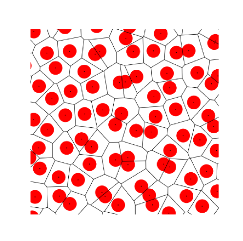
Figure 2: A disordered stealthy system decorated with spheres of radius $r$ and its Voronoi diagram. The average over the Voronoi cells of the ratio of the area outside the spheres to the total area of the cell is $E_{V}(r)$. This picture of $E_{V}(r)$ also demonstrates its relation to the covering problem, where the critical-hole radius $r_{c}$ needed to cover all space is known as the covering radius [64].

This series has a fundamental geometric interpretation, which can be seen by considering the diagram given in Fig. 2. If one has a single point configuration, this figure shows that one can compute $E_{V}(r)$ by computing the ratio of the volume outside a set of covering spheres of radius $r$ to the total volume in the process, normalized appropriately by either the fundamental cell or by averaging over the Voronoi cells [77, 78, 55, 56]. The series (23) is then just the computation of this volume fraction through the principle of inclusion-exclusion applied to the spheres. More precisely, for a single point configuration, the above series (23) becomes [64]:

$$E_{V}(r)=1-\rho v_{1}(r)+\frac{1}{v_{F}}\sum_{i<j}v_{2}^{\rm int}(x_{ij};r)-\frac{1}{v_{F}}\sum_{i<j<k}v_{3}^{\rm int}(x_{ij},x_{ik},x_{jk};r)+\cdots,$$ (24)

where $v_{F}$ is the volume of the fundamental cell. This series is expected to truncate exactly for any periodic system with a finite basis [64], such as the face-centered-cubic lattice and the hexagonal-close-packed crystal. For example, in the case of the square and triangular lattices, this series terminates at the two-body term [64]. However, as we will discuss in Section 5, it may also truncate for special disordered systems. We apply this geometric formulation of the void nearest-neighbor functions in the numerically sampling of computer-generated 1D stealthy configurations later in the article; see the Appendix for details. In addition, this view of the void functions demonstrates their close relation to important problems in discrete geometry [64]. For example, in the covering problem, one defines the covering radius as the minimum radius of the spheres in Fig. 2 required to cover all space [64]. Then, one can define the problem as a search for the point configuration which minimizes the covering radius [64] at unit density. While the covering radius is finite for any single periodic point configuration with a finite basis, it is not necessarily finite for an arbitrary disordered point process. However, in the case of stealthy point processes, it corresponds to the critical-hole radius $r_{c}$. It is worthwhile to note that the optimal configurations for the covering problem are the triangular lattice in two dimensions and the body-centered-cubic lattice in three dimensions [64, 79]. These lattices are also the entropically favored states for stealthy systems in the ordered $\chi>1/2$ regime [6]. While we focus on the disordered regime in this paper, these optimal configurations still play an important role, since for $\chi$ close to $1/2$, the disordered stealthy configurations will show precursor characterstics of these lattices.

Interestingly, this representation also forms a series of successive upper and lower bounds, which is described by a powerful general formalism developed in Ref. [72]. For example, for a homogeneous and isotropic point process, one has [72, 31]

$$E_{V}(r) \leq 1,$$ (25)

$$E_{V}(r) \geq 1-\rho v_{1}(r),$$ (26)

and

$$E_{V}(r)\leq 1-\rho v_{1}(r)+\frac{\rho^{2}}{2}s_{1}(1)\int_{0}^{2r}x^{d-1}v_{2}^{\rm int}(x;r)g_{2}(x)\,\rmd x,$$ (27)

where $v_{2}^{\rm int}(x;r)$ is the intersection volume of two spheres of radius $r$ a distance of $x$ apart, which is known analytically in any dimension [80]. In the first three space dimensions, these intersection volumes can be expressed, respectively, as [65]

$$\frac{v_{2}^{\rm int}(x;r)}{v_{1}(r)}=\Theta(2r-x)\left(1-\frac{x}{2r}\right) \qquad d=1,$$ (28)

$$\frac{v_{2}^{\rm int}(x;r)}{v_{1}(r)}=\frac{2}{\pi}\Theta(2r-x)\left[\cos^{-1}\left(\frac{x}{2r}\right)-\frac{x}{2r}\sqrt{1-\frac{x^{2}}{4r^{2}}}\right] \qquad d=2,$$ (29)

$$\frac{v_{2}^{\rm int}(x;r)}{v_{1}(r)}=\Theta(2r-x)\left[1-\frac{3}{4}\frac{x}{r}+\frac{1}{16}\left(\frac{x}{r}\right)^{3}\right] \qquad d=3,$$ (30)

where $\Theta(x)$ denotes the Heaviside step function. The last inequality (27) exactly gives $E_{V}(r)$ whenever only two-body terms contribute, such as in the case of the square and triangular lattices in 2D [64]. In the disordered case, this series can be used to derive low-$r$ expansions for $E_{V}(r)$ by expanding $g_{2}(r)$ in powers of $r$ [31]:

$$g_{2}(r)\sim a+br^{2}\qquad(r\to 0),$$ (31)

where, for the purposes of simplification, we have used in advance the fact that there is good evidence that the linear term in the preceding expansion vanishes for the types of disordered stealthy hyperuniform systems considered in this article [5, 6]. The order to which $E_{V}(r)$ can then be determined depends on the spatial dimension. In one and two dimensions, one can obtain results of the form [31, 65]

$$E_{V}(r)\sim 1-\rho v_{1}(r)+\frac{\rho^{2}a}{2}v_{1}(r)^{2}\qquad(r\to 0).$$ (32)

In three and higher dimensions, one can obtain a fourth term [31, 65]:

$$E_{V}(r)\sim 1-\rho v_{1}(r)+\frac{\rho^{2}}{2}\left(av_{1}(r)^{2}+b\frac{2d}{d+2}r^{2}v_{1}(r)^{2}\right)\qquad(r\to 0).$$ (33)

We will derive expressions for the $a$ and $b$ coefficients valid at low and intermediate values of $\chi$ in the next section.

One can repeat this analysis for $H_{V}(r),E_{P}(r),$ and $H_{P}(r).$ One obtains the following series expansions [3]:

$$H_{V}(r)=\sum_{k=1}^{\infty}(-1)^{k+1}\frac{\rho^{k}}{k!}\int g_{k}({\bi R}^{k})\frac{\partial}{\partial r}\prod_{j=1}^{k}\Theta(r-|{\bi x}-{\bi R}_{j}|)\,\rmd{\bi R_{j}},$$ (34)

$$E_{P}(r)=1+\sum_{k=1}^{\infty}(-1)^{k}\frac{\rho^{k}}{k!}\int g_{k+1}({\bi R}^{k+1})\prod_{j=2}^{k+1}\Theta(r-|{\bi R}_{j}-{\bi R}_{1}|)\,\rmd{\bi R}_{j},$$ (35)

$$H_{P}(r)=\sum_{k=1}^{\infty}(-1)^{k+1}\frac{\rho^{k}}{k!}\int g_{k+1}({\bi R}^{k+1})\frac{\partial}{\partial r}\prod_{j=2}^{k+1}\Theta(r-|{\bi R}_{j}-{\bi R}_{1}|)\,\rmd{\bi R}_{j}.$$ (36)

Note that the sequence of partial sums can be written in the form [72]:

$$W^{n}=\sum_{k=0}^{n}X^{(k)},$$ (37)

where $X$ represents one of the aforementioned functions, $X^{(k)}$ represents the $k$th term of the series for that function, and we have reindexed the series for $H_{V/P}(r)$ to start at $k=0$. Then, one obtains bounds of the form [72]

$$X\leq W^{n} \qquad n\textrm{ even,}$$

$$X\geq W^{n} \qquad n\textrm{ odd.}$$ (38)

We will explicitly use the first two successive bounds on $H_{V}(r)$ and $E_{P}(r)$ [31]:

$$H_{V}(r)\leq\rho s_{1}(r),$$ (39)

$$H_{V}(r)\geq\rho s_{1}(r)-\frac{\rho^{2}}{2}s_{1}(1)\int_{0}^{2r}x^{d-1}s_{2}^{\rm int}(x;r)g_{2}(x)\,\rmd x,$$ (40)

$$E_{P}(r)\leq 1,$$ (41)

$$E_{P}(r)\geq 1-Z(r),$$ (42)

where $s_{2}^{\rm int}(x;r)=\partial v_{2}^{\rm int}(x;r)/\partial r$ is the intersection surface area of two spheres of radius $r$ a distance $x$ apart and $Z(r)=\rho s_{1}(1)\int_{0}^{r}x^{d-1}g_{2}(x)\,\rmd x$ is the cumulative coordination number. We will also use the first bound on $H_{P}(r)$ [31]:

$$H_{P}(r)\leq\rho s_{1}(r)g_{2}(r).$$ (43)

To obtain upper (lower) bounds on $G_{V/P}(r)$, one can match an upper (lower) bound on $H_{V/P}(r)$ with a lower (upper) bound on $E_{V/P}(r)$ [31]. For example, in this paper, we will use the bounds [31]:

$$G_{V}(r)\leq\frac{1}{1-\rho v_{1}(r)},$$ (44)

$$G_{V}(r)\geq\frac{1-\frac{\rho s_{1}(1)}{2s_{1}(r)}\int_{0}^{2r}x^{d-1}s_{2}^{\rm int}(x;r)g_{2}(x)\,\rmd x}{1-\rho v_{1}(r)+\frac{\rho^{2}}{2}s_{1}(1)\int_{0}^{2r}x^{d-1}v_{2}^{\rm int}(x;r)g_{2}(x)\,\rmd x},$$ (45)

$$G_{P}(r)\leq\frac{g_{2}(r)}{1-Z(r)}.$$ (46)

As in the case of $E_{V}(r)$, one can use an expansion for $g_{2}(r)$ to derive low-$r$ expansions for all of the nearest-neighbor functions. In one and two dimensions, one finds [31]

$$H_{V}(r)\sim\rho s_{1}(r)-\rho^{2}av_{1}(r)s_{1}(r) \qquad(r\to 0),$$ (47)

$$G_{V}(r)\sim 1+(1-a)\rho v_{1}(r) \qquad(r\to 0),$$ (48)

$$E_{P}(r)\sim 1-\rho av_{1}(r) \qquad(r\to 0),$$ (49)

$$H_{P}(r)\sim\rho as_{1}(r) \qquad(r\to 0),$$ (50)

$$G_{P}(r)\sim a \qquad(r\to 0).$$ (51)

In three dimensions, one finds [31]

$$H_{V}(r)\sim\rho s_{1}(r)-\rho^{2}\left[av_{1}(r)s_{1}(r)+\frac{24b}{5}rv_{1}(r)^{2}\right] \qquad(r\to 0),$$ (52)

$$G_{V}(r)\sim 1+(1-a)\rho v_{1}(r)-\frac{8\rho b}{5}r^{2}v_{1}(r) \qquad(r\to 0),$$ (53)

$$E_{P}(r)\sim 1-\rho\left(av_{1}(r)+\frac{3b}{5}r^{2}v_{1}(r)\right) \qquad(r\to 0),$$ (54)

$$H_{P}(r)\sim\rho\left(as_{1}(r)+\frac{12b}{5}rv_{1}(r)\right) \qquad(r\to 0),$$ (55)

$$G_{P}(r)\sim a+br^{2} \qquad(r\to 0).$$ (56)

2.2 Stealthy Hyperuniform Point Processes

The stealthy constraint given by Eq. (5) only involves the two-point information contained in the point process. However, we will see it has implications for the form of the nearest-neighbor functions, which incorporate higher-order information [72]. The configurational space of all stealthy systems [defined by (5)] is infinitely large in the thermodynamic limit and extremely complex, so we make a practical restiction of our focus to a specific distribution over this space: the canonical ensemble as $T\to 0$ [5, 6]. We will see that the study of this well-defined ensemble provides powerful generic insights about stealthy systems.

2.2.1 Basic Definitions for Point Processes

We introduce the general concepts applicable to all point processes we will encounter throughout this article, using definitions that, while not completely mathematically rigorous, will be sufficient for our purposes. One can think of a $d$-dimensional point process as a configuration consisting of a countably infinite number of points in $\mathbb{R}^{d}$ such that the density is well-defined [5]. If one has an ergodic process, one can compute statistics of the point process such as the pair correlation function $g_{2}(r)$ through either a volume average over a single point configuration or through an ensemble average over many such configurations [65]. One important class of ordered point processes are known as lattices, which are point processes described by a set of linearly independent lattice vectors $\{{\bi v}_{i}\}$ in $\mathbb{R}^{d}$. The points are placed at the integer combinations of these lattice vectors, so that the location of an arbitrary point is described by the expression:

$${\bi r}=\sum_{i=1}^{d}m_{i}{\bi v}_{i}\qquad m_{i}\in\mathbb{Z}.$$ (57)

One can generalize this notion to describe a periodic point process, which is an arbitrary crystal, by including a finite set of basis vectors ${\bi b}_{n}$, which describe the position of the particles in the fundamental cell given by the lattice vectors. Thus, the points of the crystal are given by the union of the sets $\{{\bi r}_{n}\}$, where the members of the set for each $n$ are given by

$${\bi r}_{n}=\sum_{i=1}^{d}m_{i}{\bi r}_{i}+{\bi b}_{n}\qquad m_{i}\in\mathbb{Z}.$$ (58)

One can then think of a disordered point process as one in which both the size of the basis set and the volume of the fundamental cell grows to infinity, leaving the density fixed.

2.2.2 Computer Simulation

The above definition and ensemble lends itself easily to computer simulation. We will use the collective-coordinate procedure pioneered in Refs. [5, 6] for producing ground states in the canonical ensemble. Consider a finite system with $N$ particles under periodic boundary conditions. Then, the structure factor can be evaluated at every ${\bi k}$ in the reciprocal lattice of the fundamental cell with the equation

$$S({\bi k})=\frac{1}{N}\left|\sum_{i}e^{-i{\bi k}\cdot{\bi r}_{i}}\right|^{2},$$ (59)

where the sum ranges over all the particles in the fundamental cell and ${\bi r}_{i}$ is the position of the $i$th particle. Note that ${\bi k}=0$ in the above sum corresponds to the forward scattering, and is correspondingly omitted from the definition of stealthy hyperuniformity. In addition, observe that the structure factor has an intrinsic inversion symmetry:

$$S({\bi k})=S(-{\bi k}).$$ (60)

One can then define a many-particle system in which the particles interact with energy function [6]

$$\Phi=\frac{1}{v_{F}}\sum_{k<|{\bi k}|\leq K}NS({\bi k})-\Phi_{0},$$ (61)

where the sum ranges over the $M$ independently constrained wavevectors and $v_{F}$ is the volume of the fundamental cell. The constant $\Phi_{0}$ is determined by Parseval’s theorem, and can be written [5, 6]:

$$\Phi_{0}=\left(N(N-1)-2NM\right).$$ (62)

It is clear that all states of minimal energy $\Phi=-\Phi_{0}$ are stealthy. One can then sample the canonical ensemble by running a molecular dynamics simulation at a low temperature (usually around $2\times 10^{-4}$, $2\times 10^{-6}$, and $1\times 10^{-6}$ in 1, 2 and 3 dimensions, respectively, see the Appendix). To obtain a ground state configuration, one minimizes the energy of the molecular dynamics configuration using the L-BFGS algorithm [6]. For more details about the algorithms used to generate configurations in this article; see the Appendix.

The degree of short, intermediate, and long-range order depends on the control parameter $\chi$ defined in Eq. (6). For finite systems, we define $\chi$ as [5]

$$\chi=\frac{M}{d(N-1)},$$ (63)

where $M$ is the number of constrained degrees of freedom, $N$ is the number of particles, and $d$ is the spatial dimension. We can recover Eq. (6) by going to the thermodynamic limit [5]. It can be shown that the system undergoes a order-disorder transition at $\chi=1/3$ in one dimension [38] and at $\chi=1/2$ in two and three dimensions [36, 39, 4, 14, 15, 40, 5, 6, 42]. We will focus on the disordered low-$\chi$ regime.

3 Pseudo-hard-sphere Approximations to Nearest-neighbor Functions

We begin by deriving expressions useful at small-$r$ for the nearest-neighbor functions of our disordered stealthy point processes. These expressions are fundamentally based on the pseudo-hard-sphere ansatz described below, and are valid for small enough $\chi$. We also make heavy use of the bounding series given in Section 2. Throughout, we will compare to simulation data either taken from Ref. [12] or produced by the procedure described in the Appendix.

3.1 Basic Theory

To use the upper and lower bounds on the nearest-neighbor functions given in Section 2, we must first determine an accurate expression for the pair correlation function $g_{2}(r)$. Torquato, Zhang, and Stillinger [5] developed an analytical theory valid at sufficiently small $\chi$ in the limit of large systems, justifying their work through direct simulations of stealthy sytems. They make the ansatz that the structure factor follows the behavior of the pair correlation function of a hard-sphere system at a density related to $\chi$ [defined by (6)], namely,

$$S(k)=g_{2}^{HS}(r=k),$$ (64)

where $g_{2}^{HS}(r)$ is the pair correlation function for a hard-sphere system of diameter $K$ and packing fraction

$$\eta=\frac{\chi}{\alpha(K;K)2^{d}},$$ (65)

where $\alpha(r;R)=v_{2}^{\rm int}(r;R)/v_{1}(R)$ is the scaled intersection volume of two spheres of radius $R$ separated by $r$. This approximation closely follows the simulated $S(k)$ and $g_{2}(r)$ for $\chi\leq 0.15$ [5, 6]. We will use this approximation as a starting point to derive theories valid at small enough values of $r$. In particular, we will make use of the following low-$\chi$ expansion [5]:

$$S(k)\approx\Theta(k-K)\left(1+\chi\frac{\alpha(k;K)}{\alpha(K;K)}\right),$$ (66)

valid in any dimension. We will also use the generalized Orstein-Zernike relation [5]

$$\tilde{H}(k)=\tilde{C}(k)+\frac{\eta}{v_{1}(K/2)}\tilde{H}(k)\otimes\tilde{C}(k),$$ (67)

where $\tilde{H}(k)=S(k)-1$ and $\tilde{C}(k)=c^{HS}(r=k)$, where $c^{HS}(r)$ is the standard direct correlation function [16] for the aforementioned hard-sphere system. For a more detailed discussion of the pair statistics of disordered stealthy systems; see the Supplementary Material [74].

3.2 1D Results

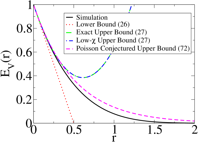
(a)

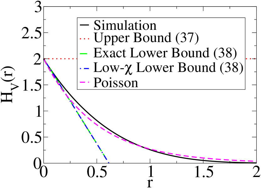
(b)

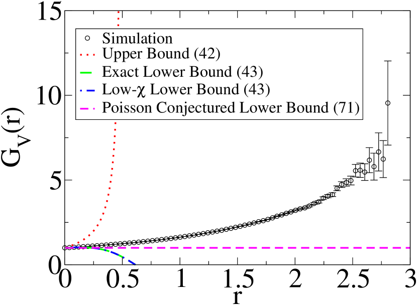
(c)

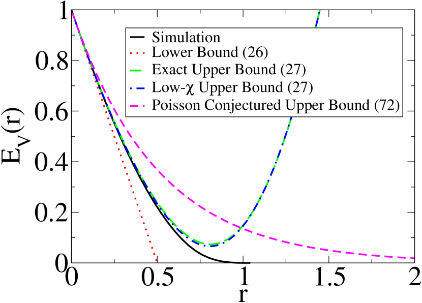
(d)

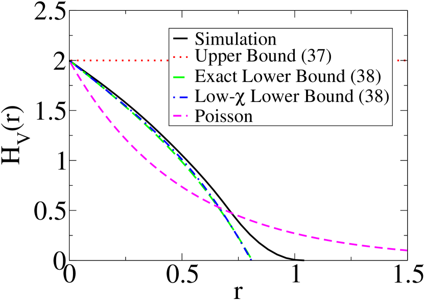
(e)

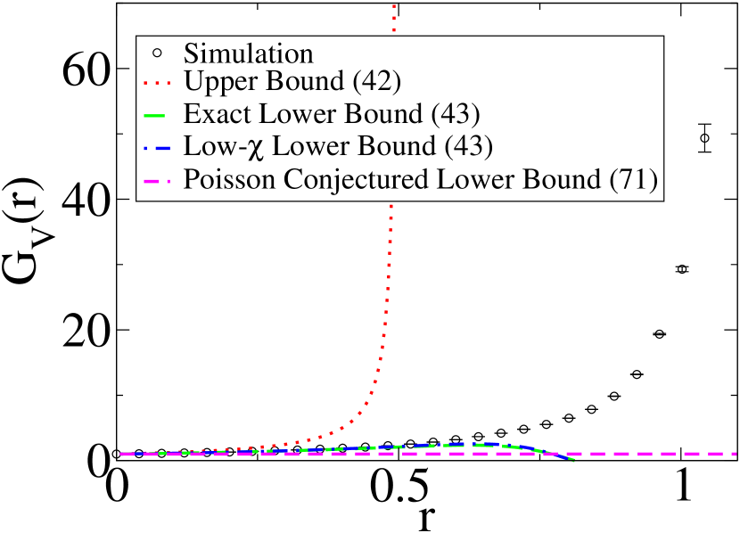
(f)

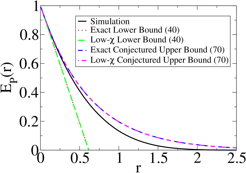
(g)

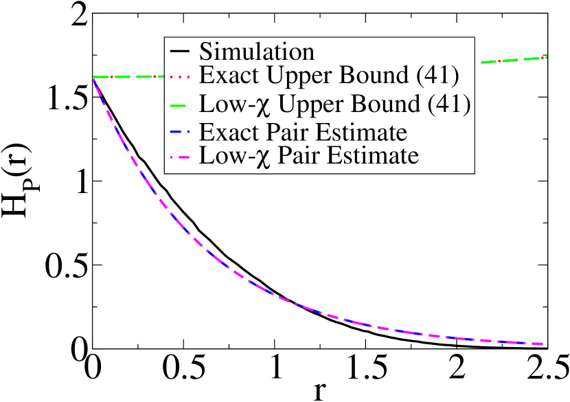
(h)

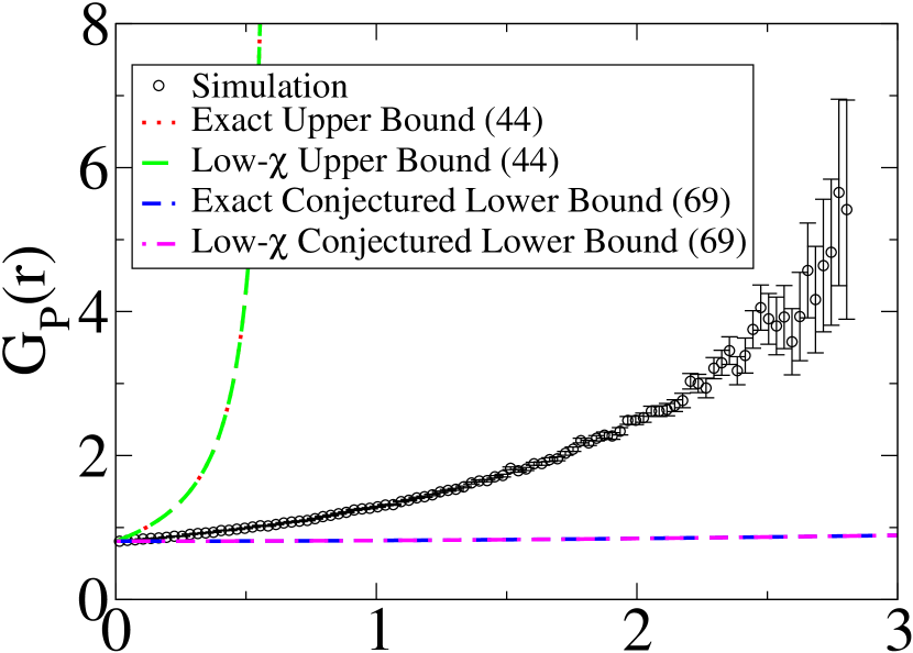
(i)

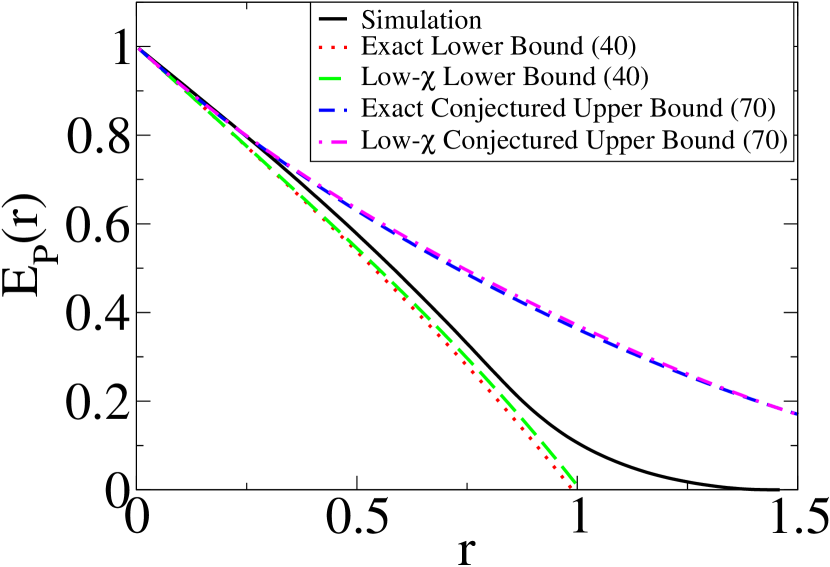
(j)

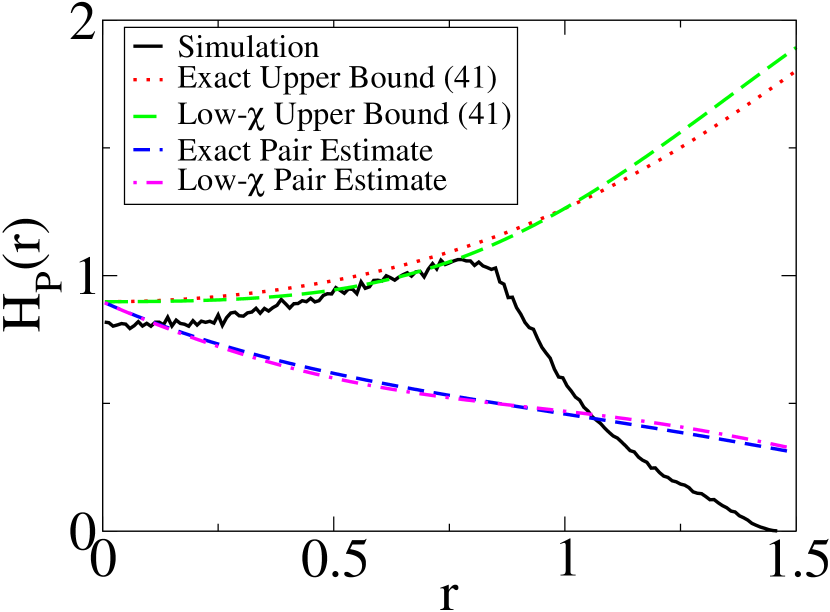
(k)

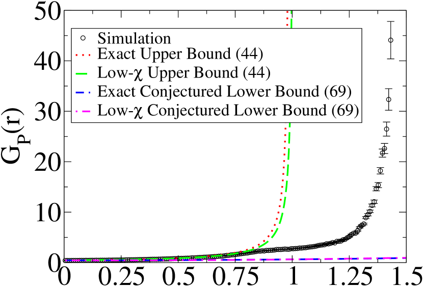
(l)

Figure 3: Bounds and approximations of the nearest-neighbor functions based on the pseudo-hard-sphere approximation for 1D stealthy systems. (a-c) Void functions for a system at $\chi=0.10$, which is within the applicability of the pseudo-hard-sphere approximation. (d-f) Void functions for a system at $\chi=0.33$, outside the applicability of the pseudo-hard-sphere approximation. (g-i) Particle functions for a system at $\chi=0.10$. (j-l) Particle functions for a system at $\chi=0.33$.

In one dimension, the expression (66) can be inverted analytically to obtain $g_{2}(r)$. We plot the results of numerically integrating this $g_{2}(r)$ with the bounds given in Section 2 in Fig. 3. We see that this approximation does quite well at low $\chi$.

Furthermore, we can derive an analytical expression for the $g_{2}(r)$ of a stealthy system using exact results for hard spheres. We take the well-known exact solution for the direct correlation function of a hard-rod system and interpret it as the Fourier transform of the direct correlation function for the stealthy system [5]:

$$\tilde{C}(k)=-\Theta(K-k)\frac{1-\chi k/K}{(1-\eta)^{2}}.$$ (68)

.

We used this expression in Eq. (67), and analytically took the Fourier inversion. The resulting expression for $g_{2}(r)$ was used to evaluate the bounds in Section 2 through numerical quadrature. In Fig. 3, we verify that these expressions form upper bounds at low $\chi$ as expected. In addition, they remain useful approximations for the void quantities even when the pseudo-hard-sphere approximation for $g_{2}(r)$ breaks down at intermediate $\chi$. However, in the case of the particle quantities, the break down of the pseudo-hard-sphere approximation creates significant inaccuracies at intermediate $\chi$.

We can use the same approximation for $g_{2}(r)$ to obtain the low-$r$ series for the nearest-neighbor functions. We obtain the coefficient $a$:

$$a=1-2\chi+\chi^{2}.$$ (69)

For reference, we also show two tentative upper bounds, yet to be proven rigorously, even in the pseudo-hard-sphere approximation. Note that combining Eqs. (9) and (11) gives [3]

$$E_{V/P}(r)=\exp\left(-\rho s_{1}(1)\int_{0}^{r}x^{d-1}G_{V/P}(x)\,\rmd x\right).$$ (70)

Now, we make a conjecture based on observations from simulations (see the Supplementary Material [74] for details), that

$$G_{P}(r)\geq g_{2}(r),$$ (71)

yielding the putative upper bound

$$E_{P}(r)\leq e^{-Z(r)}.$$ (72)

While this bound was previously presented in the context of stealthy systems in Ref. [5], it was not actually proved there. It is noteworthy that the bound is not generally obeyed by any isotropic, homogeneous and ergodic point processes. Thus, its proof must involve some nontrivial feature of the stealthy process, such as its propensity to cluster to a lesser degree than a Poisson process (this can be through the observation that $g_{2}(0)<1$ for $\chi>0$). Comparison of the relation (72) to data in Fig. 3 reveals that it indeed appears to form an upper bound, as long as the pseudo-hard-sphere approximation is applicable. We can also conjecture that bounds that apply rigorously to fermionic point processes will also be valid for stealthy systems [31]:

$$G_{V}(r)\geq 1,$$ (73)

$$E_{V}(r)\leq e^{-\rho v_{1}(r)}$$ (74)

Once again, comparison to simulations suggests that this is indeed the case (Fig. 3). Note that formulas for $H_{V/P}(r)$ derived from these bounds do not bound $H_{V/P}(r)$, which can be seen in Fig. 3.

It would be of great interest to be able to prove these bounds. The right-hand side of relation (74) has a simple physical interpretation, which is the void exclusion probability of a Poisson point process [4]. Thus, our conjecture is that the void exclusion probability of a stealthy point process is bounded above by that of a Poisson point process, aligning with physical intuition that these processes do not tolerate large holes despite their disorder.

3.3 2D Results

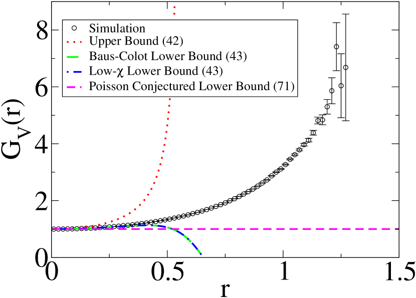
(a)

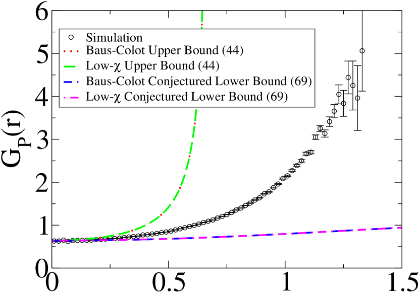
(b)

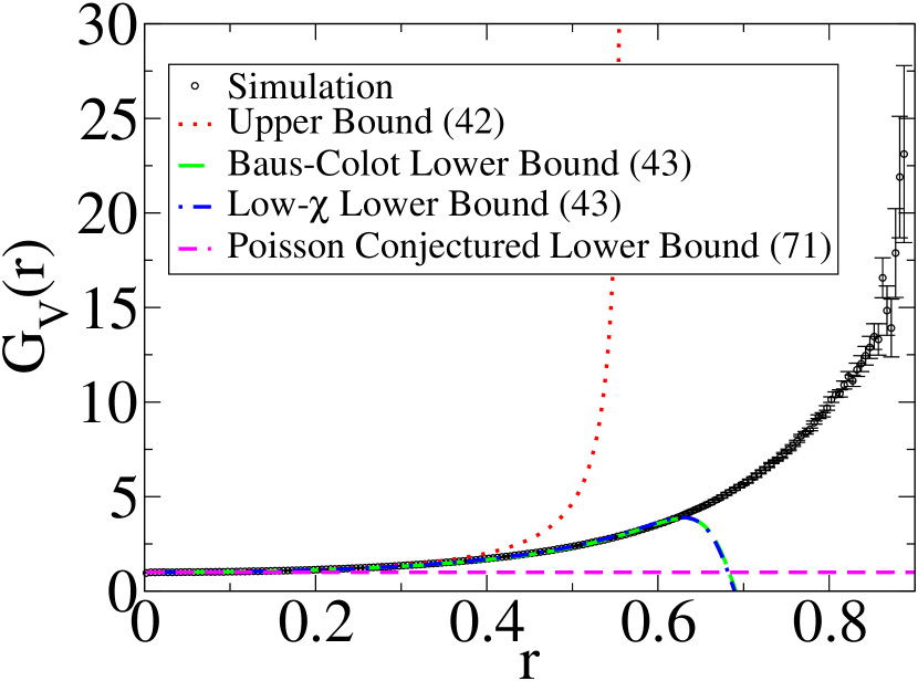
(c)

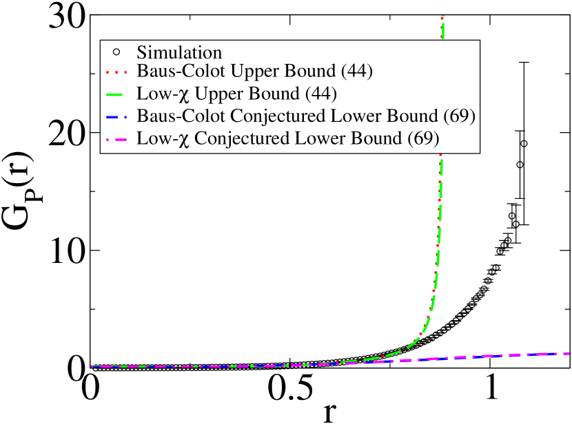
(d)

Figure 4: Bounds and approximations for the nearest-neighbor functions based on the pseudo-hard sphere approximation for 2D stealthy systems. (a-b) $G_{V}(r)$ for a system at $\chi=0.10$ and 0.33, respectively. (c-d) $G_{P}(r)$ for a system at $\chi=0.10$ and $0.33$, respectively.

In two dimensions, it is generally harder to obtain results in the pseudo-hard-sphere approximation due to the lack of exact hard-disk results. We can still use the low-$\chi$ expansion given in Eq. (66), but we must numerically invert to obtain $g_{2}(r)$. We plot the result of using this numerical $g_{2}(r)$ to evaluate the bounds in Fig. 4.

An accurate expression for the direct correlation function of 2D circular hard disks is given by Baus and Colot [81]. They begin with the low-density expansion for the direct correlation function, and make the ansatz that it describes the direct correlation function for all fluid densities so long that one uses the appropriate scaling factor. The relevant result is that we can take the Fourier transform of the direct correlation function of the stealthy system as

$$\tilde{C}(k)=-\frac{\partial}{\partial\eta}\left[\eta z(\eta)\right]\left(1-u^{2}\eta+u^{2}\eta\alpha\left(\frac{k}{u},\frac{K}{2}\right)\right),$$ (75)

where $z(\eta)=pv_{1}(K/2)/\eta k_{B}T$ is the compressibility factor of the corresponding hard-disk system and $u$ is determined by the transcendental equation

$$\frac{2}{\pi}\left(u^{2}(u^{2}-4)\sin^{-1}\left(\frac{1}{u}\right)-(u^{2}+2)\sqrt{u^{2}-1}\right)=\frac{1}{\eta^{2}}\left(1-4\eta-\left[\frac{\partial}{\partial\eta}\eta z(\eta)\right]^{-1}\right).$$ (76)

To complete this description, one must specify the compressibility factor $z(\eta)$. We use the following second-order expression from Refs. [81, 65]:

$$z(\eta)=\frac{1+\frac{7\pi-12\sqrt{3}}{3\pi}\eta^{2}}{(1-\eta)^{2}},$$ (77)

which is accurate over the relevant hard disk packing fractions. Then, we combine Eqs. (67) and (75) and take the Fourier inversion numerically to determine $g_{2}(r)$ for our stealthy systems. We plot the result of using this $g_{2}(r)$ in the approximations given in Section 2 in Fig. 4. We see that the qualitative picture is similar to the 1D case.

We can use the preceding approximation for $g_{2}(r)$ to obtain the $a$ coefficient used in the low-$r$ series for the nearest-neighbor functions. Taking $K=1$, we find that

$$a=1-\frac{{\cal U}\left(\eta\left(\left(7\pi-12\sqrt{3}\right)(\eta-3)\eta-3\pi\right)-3\pi\right)}{24\pi^{3}(\eta-1)^{3}},$$ (78)

where

$${\cal U}=\frac{\left(u^{2}+2\right)\left(-\sqrt{u^{2}-1}\right)\eta+\left(u^{2}-4\right)u^{2}\eta\csc^{-1}(u)+2\pi}{\frac{2\eta\left(\eta\left(\left(7\pi-12\sqrt{3}\right)(\eta-3)\eta-3\pi\right)-3\pi\right)\rho\left(\left(u^{2}+2\right)\left(-\sqrt{u^{2}-1}\right)\eta+\left(u^{2}-4\right)u^{2}\eta\csc^{-1}(u)+2\pi\right)}{3\pi^{2}(\eta-1)^{3}}+\rho}.$$ (79)

3.4 3D Results

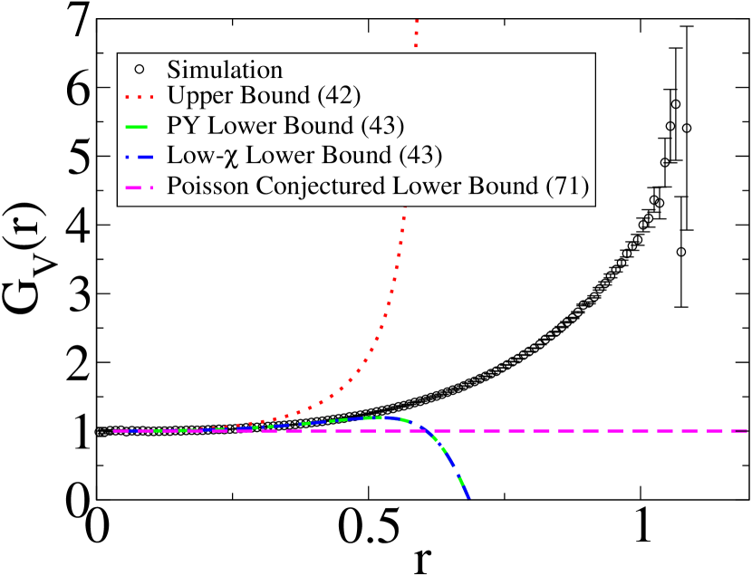
(a)

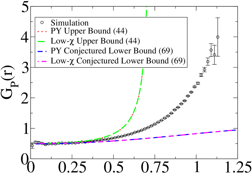
(b)

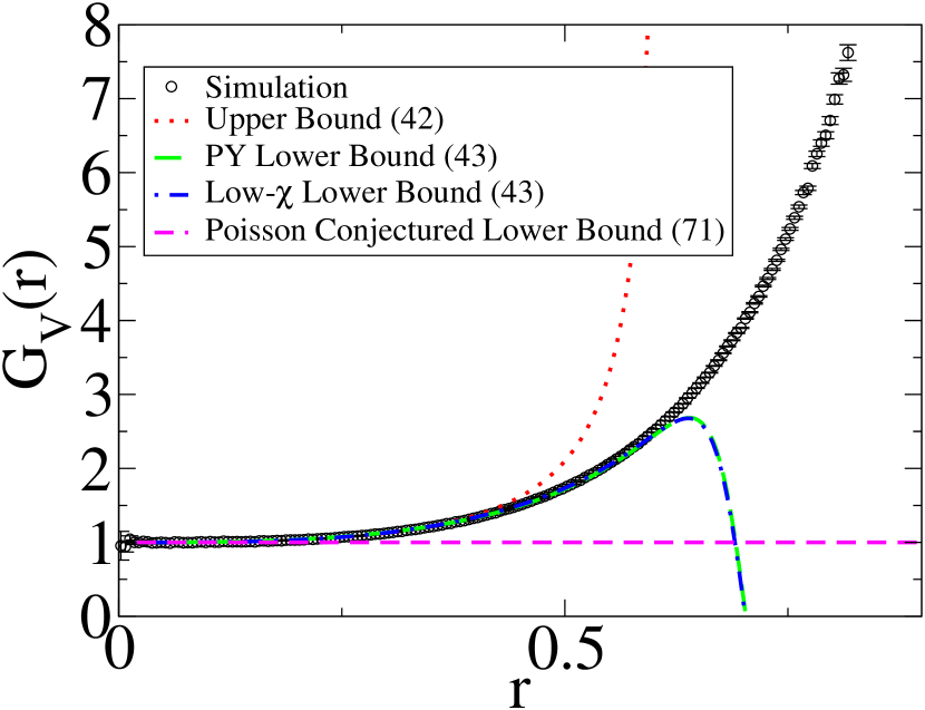
(c)

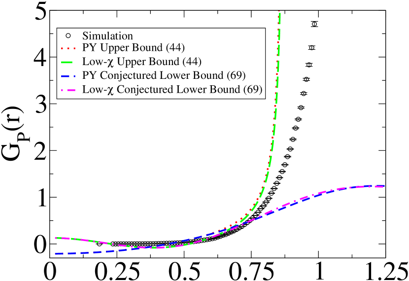
(d)

Figure 5: Bounds and approximations to the nearest-neigbor functions based on the pseudo-hard-sphere approximation for 3D stealthy ensembles. (a) Void functions for $\chi=0.10$. (b) Void functions for $\chi=0.33$. (c) Particle functions for $\chi=0.10$. (d) Particle functions for $\chi=0.33$.

Since we do not have an exact expression for $g_{2}(r)$ in 3D, we once again begin with the low-$\chi$ expansion for $S(k)$ in Eq. (66). We compute the Fourier inverse of this equation analytically, and use it to evaluate the bounds of Section 2 numerically. This is compared with simulation data in Fig. 5.

A more accurate approximation is obtained using the Percus-Yevick approximation for $g_{2}^{HS}(r)$. This gives [16]

$$\tilde{C}(k)\approx\Theta(K-k)\left(-a_{1}-6\eta a_{2}\frac{k}{K}-\frac{\eta a_{1}}{2}\left(\frac{k}{K}\right)^{3}\right),$$ (80)

where $a_{1}=(1+2\eta)^{2}/(1-\eta)^{4}$ and $a_{2}=-(1+\eta/2)^{2}/(1-\eta)^{4}$. We follow the same steps as for the 1D case with an exact $g_{2}(r)$, and compare the results to simulation in Fig 5. We find qualitatively similar trends to the 1D and 2D cases.

Using a similar argument to the 1D case, we find that the low-$r$ expansion using the PY approximation to the pseudo-hard-sphere scheme [16], taking $K=1$, is, given in terms of the coefficients for Eq. (33):

$$a=\frac{625-2750\chi+775\chi^{2}-300\chi^{3}+30\chi^{4}}{25(5+4\chi)^{2}},$$ (81)

and

$$b=\frac{3(200\chi-55\chi^{2}+8\chi^{3})(625-1000\chi+600\chi^{2}-160\chi^{3}+16\chi^{4})}{1000(5+4\chi)^{4}}.$$ (82)

3.5 Extension to Larger $\chi$

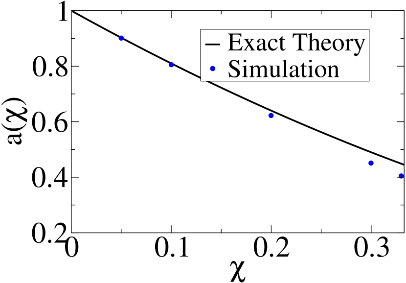
(a)

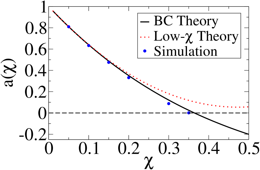
(b)

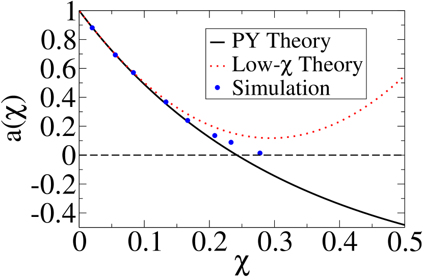
(c)

Figure 6: A comparison of the prediction for $a(\chi)$ from pseudo-hard-sphere theory to values estimated from simulation. The value of $a$ is obtained by using a quadratic extrapolation on a numerically measured $g_{2}(r)$. Data for two and three dimensions were obtained from high quality pre-existing simulations on small systems reported in Ref. [12]. (a) A comparison for 1D. As the low-$\chi$ approximation and exact solution of the pseudo-hard-sphere ansatz give the same $a$, we only show one curve. (b) A comparison for 2D. We include predictions based on the low-$\chi$ approximation and the Baus-Colot approximation. (c) A comparison for 3D. We include predictions based on the low-$\chi$ approximation and the Percus-Yevick approximation.

While the pseudo-hard sphere approximation breaks down well before the order-disorder transition at $\chi=0.5$, it is still possible to derive useful results from this approximation all the way up to the transition point. The basic observation is that while the functional form of the pair correlation function differs from the pseudo-hard-sphere approximation above $\chi\approx 0.15$ [6], the value of $g_{2}(0)$, and thus the coefficient $a$ that determines the leading order contribution to the nearest-neighbor functions, can be well modeled using a simple extension of this theory. In Fig. 6, we compare the analytical results for $a(\chi)$ given in the preceding sections to simulation data. For the 1D case, the pseudo-hard-sphere result becomes steadily worse as $\chi$ increases, but, as we will see in Section 6, this result can still be used to form a useful theory of the void functions. For the case of 2 and 3 dimensions, we see that the analytical prediction for $a(\chi)$ works very well until it crosses zero and becomes negative. In Fig. 6, we only report simulation data with a non-zero value of $a$, as our method of obtaining $a$ relies on a quadratic extrapolation that becomes invalid when $\chi$ becomes large. However, for our particular collection of finite configurations at large $\chi$, we observe $g_{2}(r)=0$ for an entire range of $r$ near origin. Thus, one can obtain a useful analytical approximation by setting $a(\chi)$ through the pseudo-hard-sphere approximation up to the zero crossing, and setting it to zero thereafter.

4 Inclusion of Higher-order Information

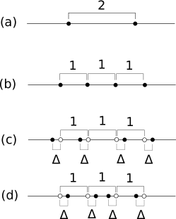
Figure 7: Clusters used to determine the highest order in the series (23) needed to evaluate $E_{V}(r)$ for the corresponding point process. (a) The least dense cluster of two particles for a one-dimensional saturated RSA process with particles of unit diameter. (b) The densest cluster of four particles for the same RSA process. (c) One of the degenerate least dense clusters of four particles for the one-dimensional perturbed lattice described in the text. The open circles represent the underlying lattice locations, while the filled circles represent the points of the configuration. (d) The one of the degenerate least dense clusters of four particles for the same perturbed lattice.

In the previous section, the results were derived using only the one and two-point correlation functions. However, as can be seen in series such as Eq. (23), the nearest-neighbor functions in principle depend on the $n$-point correlation functions $g_{n}({\bi r}^{n})$ up to arbitrary order in the infinite system size limit. In this section, we will discuss conditions under which series of this nature can be truncated using the bounded holes property, so that $E_{V}(r)$ is determined by a finite number of terms in Eq. (23). This discussion also applies to single finite configurations using the series (24), in which case the key observation is that the series can be truncated far before the last $v_{N}^{\rm int}({\bi r}^{N})$ term.

The bounded holes property plays a fundamental role in the truncation of this series. This can be seen in the following way. If one has a condition that prevents arbitrary clustering of points, such as a requirement to be a packing [64], one can show that the series in Eq. (23) must terminate after a finite number of terms for any given value of $r$. The bounded holes property lets us then extend this observation to show truncation of the series for $E_{V}(r)$ at all $r$, with an $r$-independent number of terms. Since the number of necessary terms to keep generally grows with the value of $r$ considered, the existence of a critical-hole size $r_{c}$ allows us to compute the number of terms needed by finding the number of terms needed to evaluate $E_{V}(r_{c})$. Thus, the preceding argument shows that the series (23) must terminate for any packing with the bounded hole size property. This argument has been used to show the truncation of the series (24) for all crystals [64], but we note that it applies equally to the series (23) for random sequential addition at saturation.

We can also show the truncation property for the case of stealthy point processes. To do this, we use the anti-concentration property proved in Ref. [2]. This states that for a box of side length $C/K$, the number of particles in the box is bounded above by $C^{\prime}\rho/K^{d}$, where $C$ and $C^{\prime}$ are generic constants [2]. Since stealthy systems have bounded hole sizes, it is once again sufficient to consider $E_{V}(r_{c}).$ Since we have the strict upper bound on the number of particles in a large enough box, we can also bound the maximum number of particles contained in the decorated sphere surrounding each particle in the geometric interpretation given in Fig. 2. Thus, the series must terminate after a finite number of terms. Note, however, that the number of terms that we may need to consider in the series expansion (23) increases with decreasing $\chi$.

This last observation raises an interesting fundamental question concerning the number of terms of Eq. (23) needed to describe a stealthy system. While we are not aware of a method to solve this problem analytically for disordered stealthy systems, we present analytical solutions for two interesting systems with the bounded holes property: the case of one-dimensional random sequential addition at saturation and a specific one-dimensional perturbed lattice.

For 1D random sequential addition at saturation, the truncation property is established by the previous general principle concerning packings. One can find that the series truncates at the $g_{2}(r)$ term by considering the two local configurations of four particles (or clusters) given in Fig. 7. We will take the diameter of the spheres to be unity. The first cluster shows that $r_{c}=1$ in this system, since starting at a separation of two, one can insert another particle between the neighbors, contradicting the saturation assertion. The second cluster represents the densest cluster possible while respecting the packing condition. Overlaying the covering spheres as in Fig. 2 readily shows that one only needs to consider up to intersections of two covering spheres, which corresponds to the $g_{2}(r)$ term.

The perturbed lattice we will consider is a one-dimensional lattice of unit spacing where the points (indexed by $i$) are displaced by independent random variables $\delta_{i}$ are independently drawn from an arbitrary distribution with compact support over $[-\Delta,\Delta]$. We further restrict $0<\Delta<1/2$, to prevent transposition of particles. It is interesting to note that this system is hyperuniform [82], but not stealthy hyperuniform. One should also be aware that this is very specific case of a perturbed lattice; in general, one can have correlations between the $\delta_{i}$ or unbounded displacement distributions [82]. The series (23) truncates by virtue of this system being a packing with a bounded hole size. One can see this by considering Fig. 7. The first cluster shows that $r_{c}=(1+2\Delta)/2$, while the second cluster shows that the system can be considered a packing, since there is always a gap of $1-2\Delta$ between the particles. These clusters also show that the number of terms needed is dependent on $\Delta$. For $\Delta\in(0,1/4]$, one only needs up through the $g_{2}(r)$ term, however, for $\Delta\in(1/4,1/2)$, one requires the addition of the third order term.

$\chi$	Highest Order in Series (24)
0.050	16
0.10	10
0.20	6
0.30	5
0.33	4

Table 1: A table containing the highest order necessary to evaluate $E_{V}(r)$ through the series (24) for 1D stealthy systems at various $\chi$.

The number of terms needed for stealthy systems in the series (24) can be determined numerically. While this is computationally expensive in two and higher dimensions, it can be determined in an efficient manner in one dimension by using the fact the intersection volume of $n$ 1D spheres can be written as the intersection volume of the two spheres farthest apart in the collection. The interested reader can refer to the Appendix for details. We have reported the highest order needed for our 1D stealthy systems in Table 1. We see that the number of terms needed increases with decreasing $\chi$, as predicted from the general argument above. We expect this trend to continue in higher dimensions.

5 Behavior on Approach to Critical-Hole Size

One of the surprising yet fundamental properties of any stealthy system is a bounded hole size [1, 2]. This in turn implies that $E_{V}(r)$ and $H_{V}(r)$ have compact support and that $G_{V}(r)$ diverges as it approaches the critical-hole size. We investigate the asymptotic behavior of the nearest-neighbor functions as they approach this maximum hole size, using simple theoretical arguments and computer simulations as our primary tools.

5.1 Fundamental Considerations

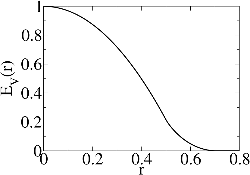
(a)

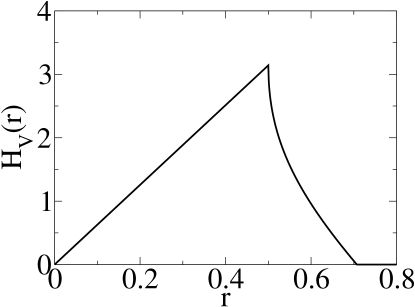
(b)

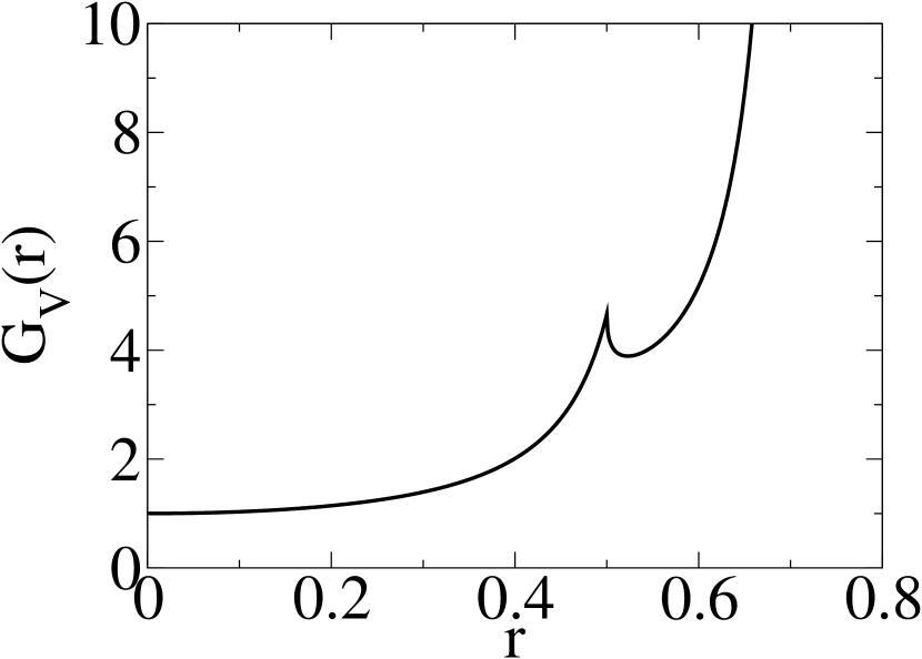
(c)

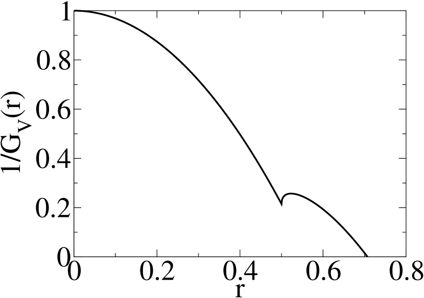
(d)

Figure 8: The nearest-neighbor functions for a square lattice. We can see that $E_{V}(r)$ and $H_{V}(r)$ have compact support, which we know is guaranteed by stealthiness. (a) The void exclusion probability decays with a power law with exponent $\gamma=2$. (b) The previous behavior of $E_{V}(r)$ implies a linear decay of $H_{V}(r)$. (c) We see that $G_{V}(r)$ diverges with a pole of order one. (d) By plotting $1/G_{V}(r)$, we can ascertain the asymptotic behavior of the other functions by the slope of the linear zero-crossing.

It is useful to generally classify the asymptotic behavior of the nearest-neighbor functions as they approach the critical-hole size. One begins with the study of crystals, which are both trivially stealthy due to the presence of Bragg peaks and have a trivially bounded hole size which is found by identifying the location of the “deep holes” in the crystal [79]. In this case, the hole probability function decays to zero as a power law [64]

$$E_{V}(r)\sim C(r_{c}-r)^{\gamma}\qquad(r\to r_{c}^{-}),$$ (83)

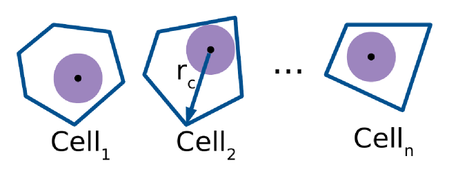
Figure 10: A schematic of Voronoi cells and spherical covering areas that demonstrates that the $E_{V}(r)$ of a crystalline system decays as a power-law with exponent $\gamma=d$ close to the critical-hole size. A crystal has a finite number of distinct Voronoi cells, and thus there exists a gap between the set of vertices at a distance $r_{c}$ and the next farthest set of vertices. Thus, we can conclude the proposed behavior through considering the decrease in volume of a small uncovered corner.

where $\gamma$ is a positive exponent. It is possible to compute the exponent of this power law analytically in the case of a crystal, and it takes the value $\gamma=d$ for spatial dimension $d$ [64]. To see this, note that there are a finite number of distinct Voronoi cells (Fig. 10), so we can always find the set of deepest holes in the system, and no other hole will be infinitesimally close to being as deep. In the intepretation of $E_{V}(r)$ as the ratio of the uncovered volume to the total volume (Fig. 2), the uncovered volume around these holes will vanish according to a power law consistent with the dimension of the system as the covered radius grows larger. In practice, this characteristic $\gamma=d$ power-law decay is most easily observed in systems with high degrees of crystallographic symmetry. Examples include lattices and crystals with only a few particles in the basis such as the hexagonal close-packed crystal. As the number of particles in the smallest basis increases, the domain in which this power law is guaranteed to be found shrinks, and disappears as the basis grows to infinity.

The asympotic form (83) then implies

$$H_{V}(r)\sim\gamma C(r_{c}-r)^{\gamma-1} \qquad(r\to r_{c}^{-})$$ (84)

$$G_{V}(r)\sim\frac{\gamma}{\rho s_{1}(r)(r_{c}-r)} \qquad(r\to r_{c}^{-}).$$ (85)

The behavior of $G_{V}(r)$ is particularly interesting. It diverges with a pole of order one, which we will see is a generic feature of the $G_{V}(r)$ of stealthy systems. For the case of the disordered stealthy systems studied here, it is a reflection of the fact that we are taking the limit $T\to 0$ while the pressure remains positive [5] (Eq. (13)). We can visualize the near-$r_{c}$ behavior of these functions easily by plotting $1/G_{V}(r)$ (Fig. 8). We see that a linear decay of $1/G_{V}(r)$ with a specified relation between the slope to the zero crossing is associated with a crystal-like power law decay.

However, in the disordered case, we find that the exponent is typically not given by $\gamma=d$. One in general expects to find a larger value, implying that the holes vanish more quickly as one approaches $r_{c}$, and we first give an intuitive argument for this fact. Since the number of distinct Voronoi cells is infinite in the general disordered case, it is possible to have a continuum of vertices with distances close to $r_{c}$. While the deepest hole in each cell still closes with the characteristic $\gamma=d$ power-law decay, the fraction of uncovered holes is also decreasing as one gets closer to $r_{c}.$ This is in contrast with the crystalline case, where the gap between the farthest and next-to-farthest vertex ensures that this fraction is constant. Thus, we expect the hole probability to reach zero asymptotically faster in the case of a disordered system, since one is both covering up volume and decreasing the fraction of cells in which there are uncovered holes near $r_{c}.$

While we are not aware of a method to compute the exponent $\gamma$ analytically in the case of a disordered stealthy system, we will work through the two examples of non-stealthy systems with bounded holes introduced in Section 4, and verify that $\gamma>d$. In the case of a one-dimensional random sequential addition process at saturation, one has that the void exclusion probability assuming spheres of unit diameter is given by [46]

$$E_{V}(r)=1-2(1-r)\int_{0}^{\infty}\frac{H(t)}{t^{2}}\,\rmd t-2\int_{0}^{\infty}\frac{H(t)}{t^{3}}\left[1-e^{-(2r-1)t}\right]\,\rmd t,$$ (86)

where

$$H(t)=e^{-2[\gamma_{e}-{\rm Ei}(-t)]},$$ (87)

where $\gamma_{e}$ is Euler’s constant and ${\rm Ei}(t)$ is the exponential integral. We then expand the exponential in the second integrand around $r=1$ and find

$$E_{V}(r)\sim 4(1-r)^{2}\int_{0}^{\infty}\frac{H(t)e^{-t}}{t}\,\rmd t+\cdots\qquad(r\to 1^{-}),$$ (88)

where we have crucially used the fact that

$$\int_{0}^{\infty}\frac{H(t)}{t^{2}}\,\rmd t=2\int_{0}^{\infty}\frac{H(t)e^{-t}}{t^{2}}\,\rmd t,$$ (89)

which can be shown by integration by parts. Thus, for this one-dimensional disordered process, the exponent $\gamma$ has increased to $\gamma=d+1$. One interesting but currently unresolved question is whether the formula $\gamma=d+1$ holds for saturated RSA processes in all dimensions.

Figure 9: The gap distribution function $p(z)$ for the one-dimensional perturbed lattice described in the text.

The approach implicitly used above by taking results from Ref. [46] is also of fundamental theoretical interest. Thus, we will now describe it in some detail, and derive new general results concerning the near-$r_{c}$ behavior of the functions involved. In one dimension, we analyze systems by introducing the gap distribution function $p(z)$, which gives the probability density to observe a gap with length between $z$ and $z+dz$ between neighboring particles [31]. Since one can relate [46, 31]

$$E_{V}(r)=\rho\int_{2r}^{\infty}p(z)(z-2r)\,\rmd z,$$ (90)

one can derive the near-$r_{c}$ behavior of $p(z)$ for systems with bounded holes by expanding around $r=r_{c}$:

$$E_{V}(r)=2\rho p(2r_{c})(r_{c}-r)^{2}+\frac{4\rho}{3}\frac{d}{dz}p(z)\bigg{|}_{z=2r_{c}}(r_{c}-r)^{3}+\cdots.$$ (91)

From this expansion, it is seen that if $E_{V}(r)$ decays with a power law with exponent $\gamma=n$ as $r\to r_{c}$, then $p(z)$ decays as a power law with exponent $\gamma=n-2$ as $z\to 2r_{c}$.

We apply this observation to determine the asymptotic behavior of the 1D perturbed lattice considered in Section 4, given a specific form of the displacement distribution. As a concrete example, we consider a uniform displacement distribution. By using the fact that the gap between particles $i$ and $i+1$ can be written in terms of the displacement variables of Section 4 as $z=1-\delta_{i}+\delta_{i+1}$, and that the distribution of the sum of independent random variables is the convolution of their individual distributions [83], one can verify that the gap distribution of this system is that given in Fig. 9. Upon inserting this form of $p(z)$ into Eq. (90) and expanding around $r=r_{c}=(1+2\Delta)/2$, we find that

$$E_{V}(r)\sim\frac{(r_{c}-r)^{3}}{3\Delta^{2}}\qquad(r\to r_{c}^{-}).$$ (92)

Thus, this 1D system has a power-law decay of $E_{V}(r)$ with exponent $\gamma=d+2.$ However, we emphasize that this system is a special type of perturbed lattice, with a specific bounded displacement distribution and uncorrelated displacements. It is clear from Eq. (91) that one can obtain any $\gamma\geq 2$ by specifying the asymptotic behavior of $p(z)$, but it would be interesting to also determine whether adding correlations between displacements or going to higher spatial dimensions would change the result.

The intuitive argument for the increase of the exponent $\gamma$ also suggests another intriguing possibility, which we will use in Section 6. In principle, one can have that the hole probability function decays faster than any power law. One simple functional form that exhibits this asymptotic behavior is [84]:

$$E_{V}(r)\sim C\exp\left(-\frac{\zeta}{r_{c}-r}+\cdots\right)\qquad(r\to r_{c}),\\$$ (93)

giving rise to the following asymptotic forms for $H_{V}(r)$ and $G_{V}(r)$:

$$H_{V}(r)\sim\left(\frac{\zeta C}{(r_{c}-r)^{2}}+\cdots\right)\exp\left(-\frac{\zeta}{r_{c}-r}+\cdots\right) \qquad(r\to r_{c})$$ (94)

$$G_{V}(r)\sim\frac{\zeta}{\rho s_{1}(r)(r_{c}-r)^{2}}+\cdots \qquad(r\to r_{c}).$$ (95)

This behavior gives a divergent $G_{V}(r)$ with a pole of order two. In general, a pole of any order would be permissible, but we only explicitly consider the order two case. If we consider instead the reciprocal function $1/G_{V}(r)$, we see that a quadratic (or any higher order) decay is associated with an $E_{V}(r)$ that decays faster than any crystal on approach to the critical-hole size. It is possible to specify a specific distribution for the 1D perturbed lattice considered previously that can be shown to possess an $E_{V}(r)$ that decays faster than any power law, although we have not been able to compute the exact form of Eq. (95). One takes the displacement distribution $u(\delta)$ as

$$u(\delta)=\frac{1}{I}\exp\left(\frac{1}{\delta^{2}-\Delta^{2}}\right)\qquad-\Delta<\delta<\Delta,$$ (96)

and zero elsewhere, where $I$ is the normalization constant needed to create a well-defined probability density function. One can then verify through judicious replacements of pieces of the convolution integrand for $p(z)$ by constants that form upper bounds that $p(z)$ decays faster than any power law as $z\to 2r_{c}$. This implies through Eq. (91) that $E_{V}(r)$ also decays faster than any power law, since the coefficient for each term in the series will be zero [84, 85]. However, the use of these coarse upper bounds in the argument prevents us from extracting the exact asymptotic behavior. It would be interesting to identify a system for which a form of $G_{V}(r)$ with a higher-order pole could be exactly computed.

Given the fundamental importance of the near-$r_{c}$ behavior described above, it is essential to develop intuition for the case of stealthy systems. Since we currently lack strong enough direct theoretical tools, we provide some preliminary data via computer simulations that contextualizes these simple arguments.

5.2 Simulation Results

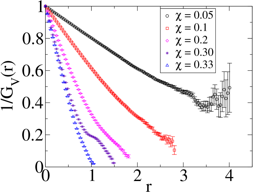
(a)

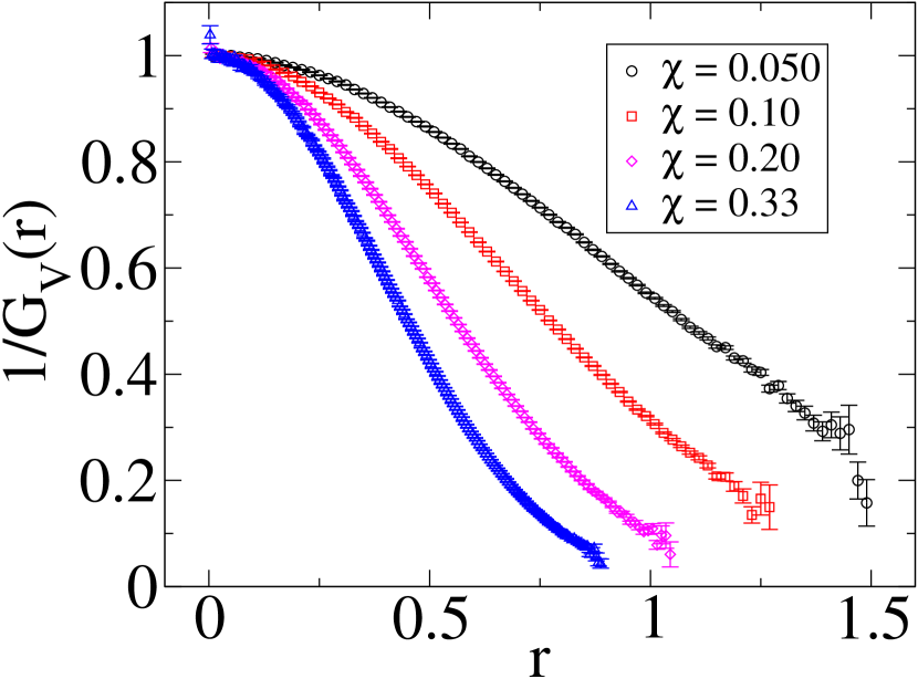
(b)

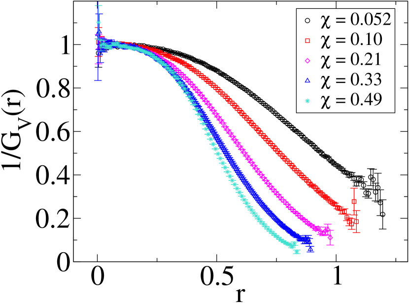
(c)

Figure 11: Simulations of $1/G_{V}(r)$ for the first three spatial dimensions. See the Appendix for details on system and ensemble size. (a) Simulations for 1D. (b) Simulations for 2D. (c) Simulations for 3D.

Here, we present simulation results for $G_{V}(r)$ in 1, 2, and 3 dimensions (Fig. 11). We sample $G_{V}(r)$ through a geometric method in 1D and by binning the nearest neighbors in 2D and 3D; see the Appendix for details. While the obtained statistics are not good enough to draw robust conclusions, in two and three dimensions, we can see the beginning of a cross-over in the form of a decreased slope for $1/G_{V}(r)$ on the larger-$\chi$ samples. This suggests that $E_{V}(r)$ for these configurations will either have power-law tails with large values of $\gamma$, or that they will have an $E_{V}(r)$ that decays faster than any power law. In one dimension, the behavior at higher-$\chi$ is somewhat more complicated, with a plateau forming at $\chi=0.20$ and disappearing in the $\chi=0.33$ data. This disappearance is likely due to a subtle finite size error, where crystallization is enhanced close to the $\chi=1/3$ order-disorder transition that exists in the thermodynamic limit [38]. Indeed, we observe that a small amount of long-order develops in the form of slowly decaying oscillations in the pair correlation function for our $\chi=0.33$ data. However, we still report these curves throughout the article, since we expect this error to be much less noticeable both in $G_{V}(r)$ far from the critical-hole size and in the less sensitive quantities $E_{V}(r)$ and $H_{V}(r)$. We observe that the likely behavior close to $r_{c}$ for $E_{V}(r)$ is a power-law decay, however, this does not necessarily imply that this is the case for all dimensions. Whether the true asympotics for $E_{V}(r)$ are power-law decays or not, these results suggest that while both crystals and disordered stealthy systems have bounded hole sizes, the functions $H_{V}(r)$ and $E_{V}(r)$ of disordered systems approach their asymptotic value much more quickly as one moves toward the critical-hole size.

This observation explains why it is extremely difficult to sample the near-$r_{c}$ behavior for disordered stealthy systems. Since $E_{V}(r)$ vanishes as the critical-hole size is approached, the faster decay implies that for any finite configuration, the event of observing a hole with size sufficiently close to the critical-hole size is rarer than that of a crystalline system. Thus, one needs to sample much larger systems, unlike in the case of a crystal, for which a single copy of the fundamental cell suffices. This observation is also closely linked to one made by Zhang, Stillinger, and Torquato [1], which is that it is easier to observe large holes for $\chi$ close to $1/2$ than for smaller $\chi$, since the relative lack of close-range order for small $\chi$ implies that the event of finding a large hole becomes correspondingly rarer.

6 Towards Accurate Expressions for Nearest-neighbor Functions Over the Whole Domain

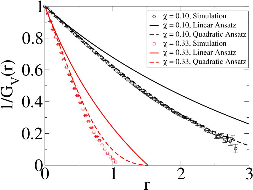
(a)

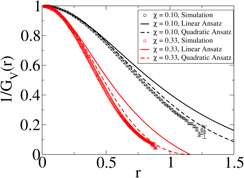
(b)

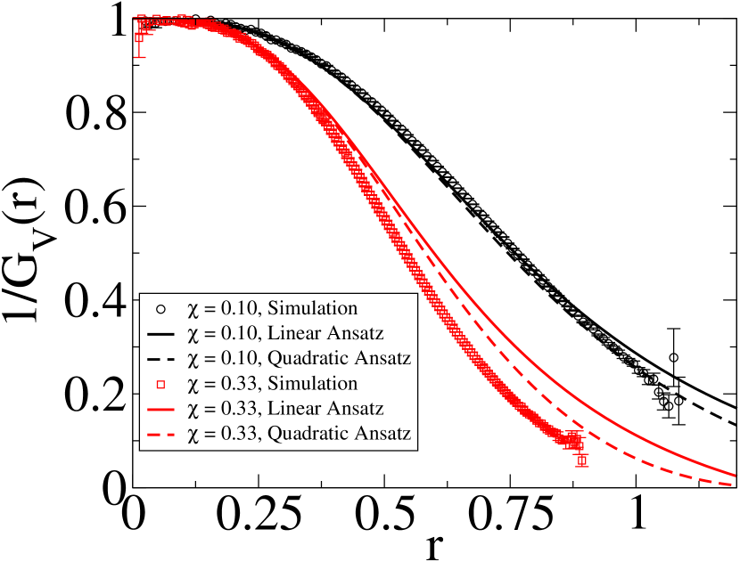
(c)

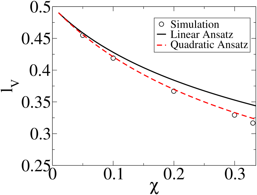
(d)

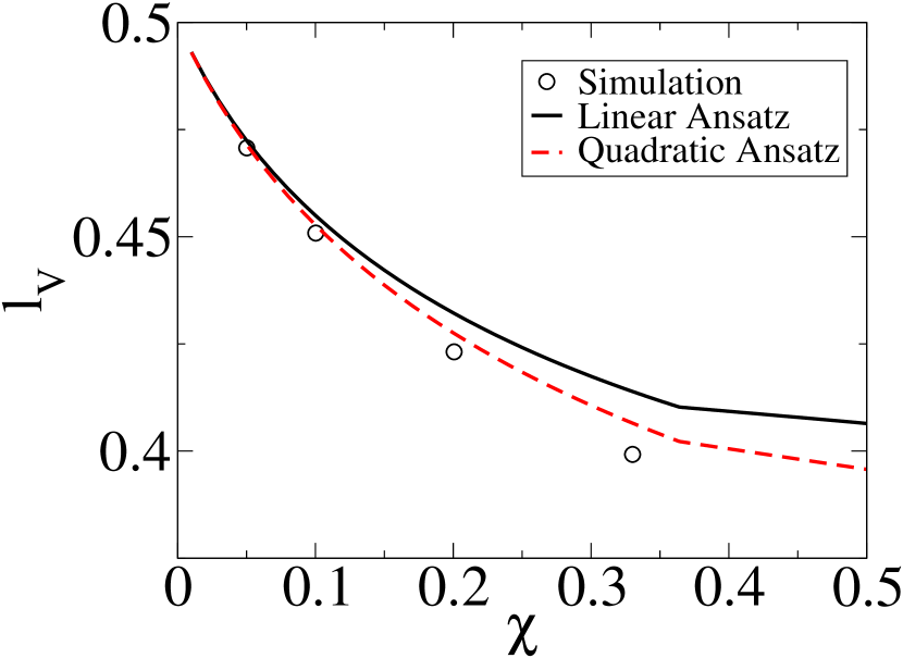
(e)

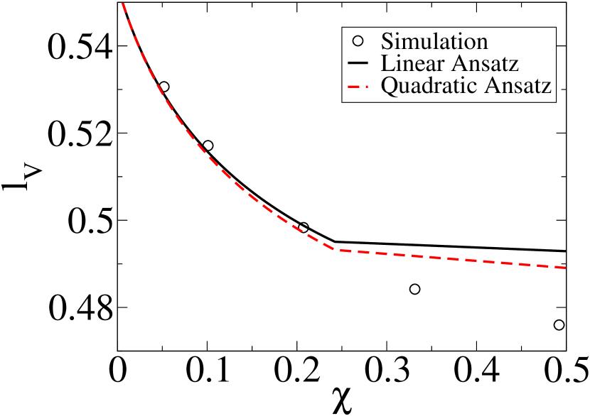
(f)

Figure 12: Comparisons between simulations and the theories given in Eqs. (97) and (98). (a-c) $1/G_{V}(r)$ for two different values of $\chi$ in one, two, and three dimensions, respectively. (d-f) The void mean nearest-neighbor distance $l_{V}$ as a function of $\chi$ for one, two, and three dimensions, respectively.

We now devise an approximation that matches the contributions to the small-$r$ and near-$r_{c}$ expressions discussed above. The basic strategy is to make a change of asymptotic scale on the small-$r$ asymptotic expansion for $G_{V}(r)$ given in Eq. (48) so that it matches either the pole-of-order-one asymptotics of Eq. (85) that gives rise to a power law decay of $E_{V}(r)$ or the pole-of-order-two asymptotics of Eq. (95) that gives rise to an exponential decay of $E_{V}(r)$ as $r$ approaches $r_{c}$. While there are many ways of doing this, one fruitful choice is to take either the pole-of-order-one formula:

$$G_{V}(r)=1+\frac{(1-a)v_{1}(r_{c})\rho v_{1}(r)}{v_{1}(r_{c})-v_{1}(r)},$$ (97)

or the pole-of-order-two

$$G_{V}(r)=1+\frac{(1-a)v_{1}(r_{c})^{2}\rho v_{1}(r)}{[v_{1}(r_{c})-v_{1}(r)]^{2}},$$ (98)

where the maximal hole size $r_{c}$ is given by the formula [1]:

$$r_{c}=\frac{(d+1)\pi}{2K}.$$ (99)

In addition to connecting behaviors consistent with the small-$r$ expansions given in Section 3 and our observations concerning the close-to-critical-hole-size regime presented in Section 5, we believe they satisfy the bounds given by the inequalities (44) and (45) (although we have not constructed a rigorous proof of this proposition). They have been compared to simulation data for $G_{V}(r)$ and $l_{V}$ in Fig. 12. We can see that in one and two dimensions, the pole-of-order-two formula (98) is more accurate, with good agreement at low-$\chi$ and tolerable agreement at intermediate $\chi$. While this formula gives different asymptotics than is apparent in the data for $1/G_{V}(r)$ for the 1D system at $\chi=0.30$ given in Fig. 11, this is likely balanced by lessening the error at smaller $r$, which dominates the contribution to $l_{V}$. In three dimensions, the two formulas give similar predictions, with the more accurate approximation being determined by the value of $\chi$. We also see that the prediction for $l_{V}$ qualititatively breaks down past a certain $\chi$, where we believe higher-order coefficients such as $b$ must be included.

7 Positive Temperature

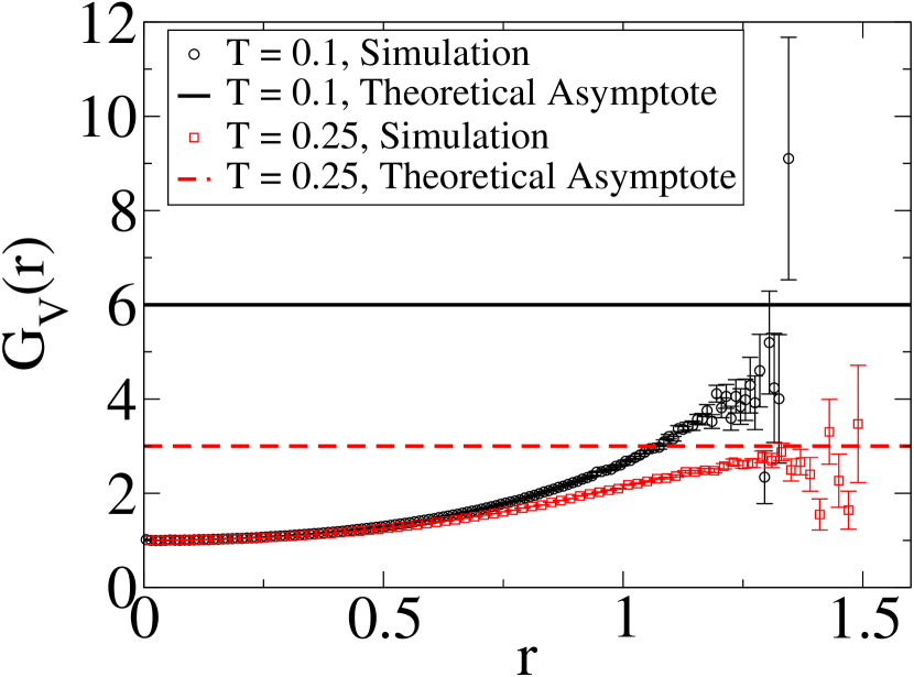
(a)

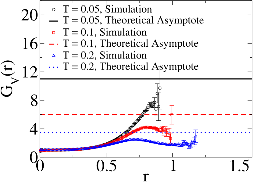
(b)

Figure 13: The function $G_{V}(r)$ sampled at positive temperatures for (a) a 2D ensemble at $\chi=0.10$ and (b) a 3D ensemble at $\chi=0.49$, as well as the saturating values predicted by Eq. (101).

For sufficiently small temperatures, we have that the pressure of a stealthy system is expliclitly given by [5]

$$p\sim\rho T+\frac{\rho^{2}v_{0}}{2}.$$ (100)

From Eq. (13), we then have a prediction for the asympotic value of $G_{V}$ as (taking $\rho=1$):

$$G_{V}(r\to\infty)\sim 1+\frac{1}{2T}.$$ (101)

Note that this formula implies that there will be a singular change in behavior of holes in the system as one increases the temperature, even infinitesimally, from $T=0$. The presence of a finite asymptote suggests that one can in principle expend an arbitrarily large amount of work to create an arbitrarily large hole. Thus, since this system is in equilibrium, the maximum hole size will be unbounded in the infinite volume limit at positive temperature. This is in stark contrast to the ground state behavior, where Eq. (101) does not apply due to the presence of the divergence. This divergence is ultimately derived from the fact that the relation between $G_{V}(r)$ and the work required to produce a hole becomes singular at $T=0$ [47].

We have plotted the results of simulations at positive temperatures for $G_{V}(r)$ in Fig. 13. However, none of these cases definitively asymptote to the predicted value before the simulated data becomes very imprecise. We are unsure whether this discrepancy is caused by the difficulty of sampling $G_{V}(r)$ at large $r$ and positive $T$, or whether the linear approximation (100) simply breaks down. We can also see that for some values of $\chi$ and $T$, the behavior of $G_{V}(r)$ can become non-monotonic.

8 Conclusions and Discussion

In summary, we have obtained bounds and approximations to the nearest-neighbor functions valid in the small-$r$ and $\chi$ regimes through the use of the pseudo-hard-sphere ansatz, formally advanced a pair of conjectured bounds, showed that the nearest-neighbor functions of stealthy systems can be determined by a finite number of $g_{n}({\bi r}^{n})$, investigated the close-to-critical-hole-size regime through theoretical arguments and simulation, and combined insights from these analyses to form an approximation valid for small $\chi$ and all $r$. We showed that disordered stealthy processes appear to possess different behavior from their ordered counterparts as they approach their critical-hole size. Finally, we have given the asymptotic behavior of $G_{V}(r)$ for finite temperature systems, and concluded that we expect stealthy systems to lose their bounded hole size property, even at arbitrarily small temperatures.

These results both answer fundamental questions about the statistical properties of stealthy hyperuniform systems and raise new avenues of inquiry. They suggest that the asysmptotic behavior of the nearest-neighbor functions near the critical-hole size is different for ordered and disordered stealthy systems, but obtaining more complete evidence in favor of this proposition will likely require the development of new methods for the investigation of stealthy systems. This may either take the form of numerical methods to sample large holes or an increase in efficiency in which these unusual potentials can be simulated, or theoretical methods to directly obtain the asymptotic behavior. In addition, the singular disappearance of a bounded hole size at positive temperature further incentivizes studies of the positive temperature regime, as one may find other unusual statistical characteristics of these systems.

In addition to the implications for these systems as point processes, those results which apply at intermediate $\chi$ can also be used to comment on the structure of disordered packings of intermediate density, as any finite stealthy system can be decorated with spheres whose diameter depends on $\chi$ to obtain a packing. Considered as two-phase systems, these packings are also stealthy hyperuniform [12].

Having outlined methods for obtaining good analytical approximations to these functions, we can then investigate applications to the field of heterogenous materials. Accurate expressions for the nearest neighbor functions can be used to place bounds on or estimate the trapping constant [67, 68, 69, 65] and fluid permeability [65] of two-phase systems derived from these point processes. These bounds may find use in identifying applications for stealthy processes in materials engineering.

Appendix A Simulation Details

In this Appendix, we give details on the numerical methods used to produce results in this article, with the exception of the two and three dimensional results given in Fig. 6, which is partially based on a resampling of data presented in Ref. [12].

A.1 Collective Coordinate Procedure

$d$	$\chi$	Figs.	$N$	$N_{\rm snap}$	$N_{\rm step}$	$N_{\rm eq}$	Unit Cell
1	0.0499	T1,6,11,12	9300	500	5000	200	Integer Lattice
1	0.10002	T1,3,6,11,12	6600	500	5000	200	Integer Lattice
1	0.1998	T1,6,11,12	4600	500	5000	200	Integer Lattice
1	0.2998	T1,6,11,12	3800	500	5000	200	Integer Lattice
1	0.3301	T1,3,6,11,12	3600	500	5000	200	Integer Lattice
2	0.0502	6,11,12,S3	9300	500	5000	200	Triangular Lattice
2	0.1002	4,6,11,12,S3,S4	6600	500	5000	200	Triangular Lattice
2	0.201	6,11,12,S3	4600	500	5000	200	Triangular Lattice
2	0.3301	4,6,11,12,S3,S4	3600	500	5000	200	Triangular Lattice
3	0.519	11,12	9300	500	5000	200	BCC Lattice
3	0.101	5,11,12,S1,S2	6600	500	5000	200	BCC Lattice
3	0.207	11,12	4600	500	5000	200	BCC Lattice
3	0.331	5,11,12	3600	500	5000	200	BCC Lattice
3	0.492	11,12	3000	500	5000	200	BCC Lattice
2	0.101	13	6600	300	5000	200	Square Lattice
3	0.491	13	2000	200	5000	600	Cubic Lattice

Table 2: A table containing simulation parameters for systems used throughout article. The figure numbers prefixed with a T refer to tables and those prefixed with an S refer to the Supplementary Material [74].

Our collective coordinate procedure is similar to the one used in Refs. [5, 6, 42, 1, 12], but with a few key differences. The first is that the the time step choice algorithm and general structure of the program has been modified. We still adjust the time step based on the log-ratio of the energy between snapshots, but the threshold depends on the total number of snapshots $N_{\rm snap}$ taken. Denote the number of steps between samples to be $N_{\rm step}$. During the initial time step choice and equilibration phase, one first evolves the system $N_{\rm step}/2$ steps, and then adjust the timestep by sending

$$\Delta t\to\left\{\begin{array}[]{l l}0.5\Delta t&\mathcal{E}>0.0005/N_{\rm snap}\\ 0.9\Delta t&0.0005/N_{\rm snap}\geq\mathcal{E}>0.0003/N_{\rm snap}\\ 0.95\Delta t&0.0003/N_{\rm snap}\geq\mathcal{E}>0.0002/N_{\rm snap}\\ 1.2\Delta t&\mathcal{E}<0.000001/N_{\rm snap}\\ 1.05\Delta t&0.000001/N_{\rm snap}\leq\mathcal{E}<0.00005/N_{\rm snap}\\ \Delta t&{\rm otherwise},\end{array}\right.$$ (102)

where

$$\mathcal{E}=\left|\frac{2\ln(E_{i}/E_{i+1})}{N_{\rm step}}\right|.$$ (103)

Then, one repeats the above $N_{\rm eq}$ times. Afterwards, one evolves the system for $N_{\rm step}/2$ using an Andersen thermostat and $N_{\rm step}/2$ without an Andersen thermostat, and takes a snapshot at the end with the L-BFGS algorithm (for ground states). One repeats this $N_{\rm snap}$ times.

We have justified this change through a blocking analysis, where we have observed that upon splitting each trajectory into five equal portions sequentially, the value of $g_{2}(r)$ observed in each sub-trajectory is similar. Whenever an uncertainty for $g_{2}(r)$ was necessary (e.g., in the extrapolation to obtain the numerical $a$ coefficient) it is estimated by assuming each snapshot contributes independently to the final value. This independence assumption was corroborated by a standard block uncertainty analysis [86]. In three dimensions, we occasionally drop the first bin of $g_{2}(r)$ because no counts are recorded, even though the likely value of $g_{2}(r)$ is not zero. This is likely a finite size effect.

The second change is that we conduct our simulations at $\rho=1$ rather than $K=1$. This has important implications for the choice of temperature used to equilibrate the system before taking snapshots. While we use the same values as Ref. [6] ($T=2\times 10^{-4},2\times 10^{-6},$ and $1\times 10^{-6}$ for one, two, and three dimensions, respectively), it should be noted that this choice actually corresponds to physically distinct systems, since changing the density changes how far the particles need to move to obtain the same difference in energy. We have justified this choice by also simulating at temperatures one order of magnitude below those stated above. We observe that $g_{2}(r)$ does not change when simulated with this lower equilibration temperature.

In general, we work with larger systems that have been equilibrated for a shorter amount of time and with fewer snapshots than the corresponding work in Refs. [5, 6, 42, 1, 12]. The values of the system size $N$, $N_{\rm snap}$, $N_{\rm step}$, and $N_{\rm eq}$ along with the shape of the unit cell of each system and a specification of which figures the data is used in, is given in Table 2.

Throughout the article, we have used the rounded values of $\chi$ appearing in the figures to compute theoretical curves. Due to the finite size effects implicit in Eq. 63, one cannot obtain exactly these values of $\chi$ with our chosen system sizes. Instead, we use a relatively close value of $\chi$, which rounds correctly to two significant figures. To give an idea of how much error is made when making this choice, we have reported the values of $\chi$ to the next non-trivial significant figure in Table 2. Figures where $\chi$ appears as the bottom axis use more precise estimates of $\chi$.

A.2 Sampling the Nearest-Neighbor Functions

For the void quantities in one dimension, we use the fact that $E_{V}(r)$ is the ratio of uncovered space to total space in Fig. 2 and that $H_{V}(r)$ is the surface area of the covered space [3]. This has been used previously to compute accurate results in two and three dimensions [55, 56, 57]. For the purposes of this article, we note that this interpretation gives rise to a simple method in 1D. In particular, we can sample the nearest neighbor function by simply compiling a list of all the gap sizes in the system, and computing the uncovered length of these gaps at each $r$. To ensure a meaningful estimate of the uncertainty in our calculation, we drop any $r$ for which fewer than 10 individual gaps contribute. The uncertainty for $H_{V}(r)$ and $E_{V}(r)$ are then computed as the standard deviation of the mean with the value from each snapshot being treated as independent. $G_{V}(r)$ is computed as the ratio, and the uncertainty propagated linearly.

For the void functions in two and three dimensions and the particle functions in all dimensions, we use a sampling strategy. One computes the function $H_{V/P}(r)$ through binning nearest neighbor observations, the function $E_{V/P}(r)$ by recording every observation where the nearest neighbor is at least $r$ away, and $G_{V/P}(r)$ by taking their ratio. Since this method involves estimating a sensitive statistical quantity through a quotient, care must be taken to reduce systematic error. To this end, we compute these quantities using multiple bin sizes, and compare them to ensure that we have obtained a stationary estimate with respect to bin size. To ensure a meaningful estimate of the uncertainty in our calculation, we drop any bin for which fewer than 10 observations contribute to $H_{V}(r)$. Uncertainties for $H_{V}(r)$ and $E_{V}(r)$ are computed by assuming each snapshot contributes independently to the final value, and the uncertainty for $G_{V}(r)$ is propagated through the ratio linearly.

We also sample $E_{V}(r)$ via the series (24) in 1D for the purpose of determining how many terms in the series is needed. To do this, we use the fact that $v_{n}^{\rm int}({\bi r}^{n})$ is just $v_{2}^{\rm int}(r)$, where $r$ is taken as the distance between the two points farthest apart. Thus, we can compute the series for $E_{V}(r)$ to arbitrary order as follows: first, compute all of the pair distances up to $r$ and the number of particles $m$ contained between the pair, and then compute the contribution of the pairs according to the formula

$$E_{V}^{ij}(r)=\sum_{k=0}^{m}(-1)^{k}{m\choose k}v_{2}^{\rm int}(r_{ij}).$$ (104)

Finally, one sums the contribution of all pairs to obtain $E_{V}(r)$. The highest order needed is then $m_{c}+2$, where $m_{c}$ is the highest $m$ value observed in the calculation for $E_{V}(r_{c})$. The value of $r_{c}$ is determined by looking for a large drop in $E_{V}(r)$, as past $r_{c}$, the value of $E_{V}(r)$ is very close to zero. This drop is typically many orders of magnitude.

References

Supplementary Material

Appendix A Comparison of Nearest-Neighbor Functions for Selected Systems

In developing intuition for the behavior of the nearest-neighbor functions, it is instructive to compare their behaviors for a variety of systems of physical importance. In Fig. S1 below, we compare the void nearest-neighbor functions for the Poisson point process, an equilibrium hard-sphere fluid, and a representative disordered stealthy hyperuniform system at intermediate $\chi$. If we focus on just $H_{V}(r)$ and $E_{V}(r)$, it may appear that the stealthy hyperuniform process falls “between” that of equilibrium hard spheres and the uncorrelated Poisson process, but inspection of $G_{V}(r)$ makes it clear that the large-$r$ behavior of the stealthy system is qualitatively different than that of the non-stealthy systems. Stealthy systems have compact support for $H_{V}(r)$ and $E_{V}(r)$ [1, 2], which manifests itself clearly as a divergence of $G_{V}(r)$ at a finite $r$. Thus, while in principle one can compute all three functions from knowledge of just one, one can obtain a clearer understanding of the behavior of a system by considering each in turn.

We plot the particle nearest-neighbor functions for the same systems in Fig. S2 of the Supplementary Material. Similar to the case of the void quantities, the divergence of $G_{P}(r)$ is indicative of the bounded hole property of stealthy systems. It is also important to note that the determination of the particle properties is in some sense “harder” for stealthy systems than for previously investigated systems. While there are fundamental symmetries in the Poisson process and equilibrium hard-sphere fluid systems that allow for the determination of the particle from the void quantities [3], no such symmetry exists in our stealthy hyperuniform systems.

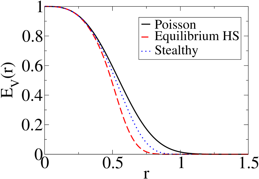
(a)

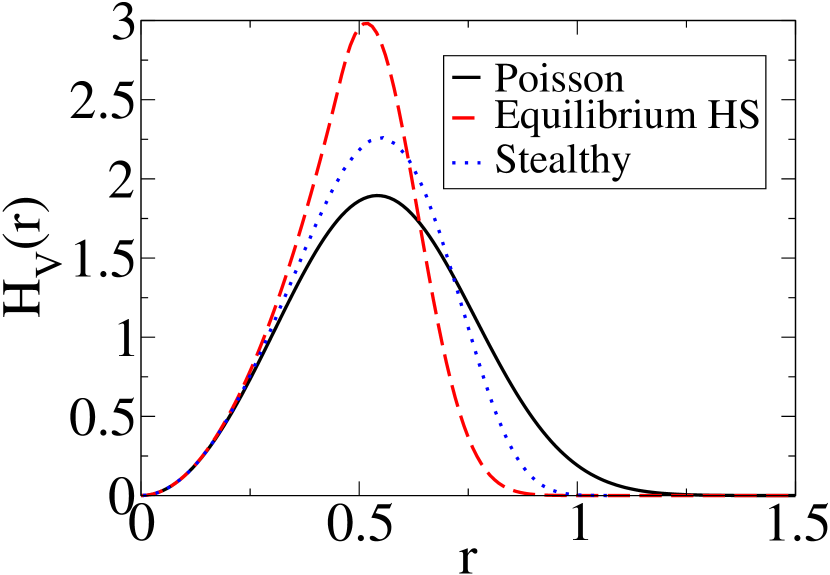
(b)

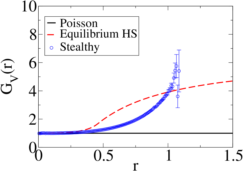
(c)

Figure S1: The void nearest-neighbor functions $E_{V}(r)$, $H_{V}(r)$, and $G_{V}(r)$ for a Poisson point process at $\rho=1$, an equilibrium hard-sphere system at $\rho=1$ and $\phi=0.4$, and a stealthy ensemble at $\rho=1$ and $\chi=0.10$. The Poisson results were computed with an exact formula [4], the hard-sphere system was computed with an accurate approximation based on the Carnahan-Starling formula [3], and details concerning the stealthy ensemble can be found in the Appendix of the main article. (a) and (b) We can see that the Poisson process as the widest distribution of hole sizes and nearest-neighbor distances. (c) The bounded hole size property of the stealthy ensemble can be clearly seen in the divergence of $G_{V}(r)$.

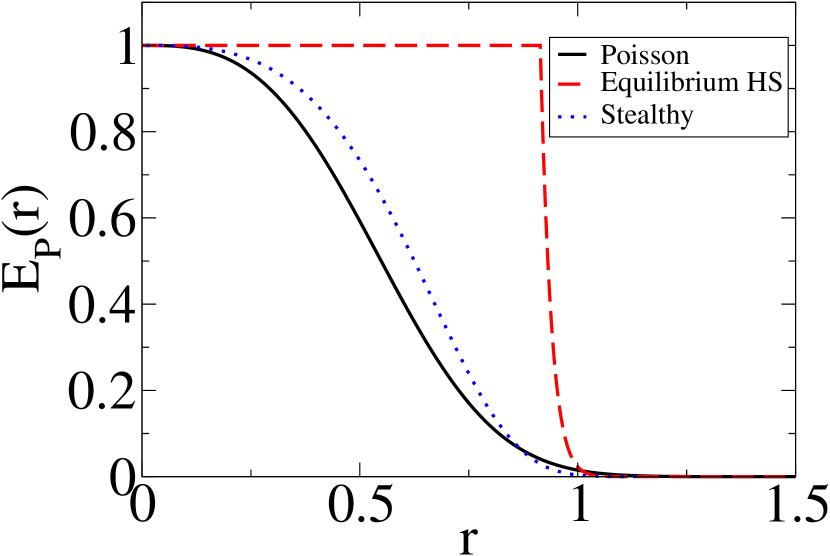
(a)

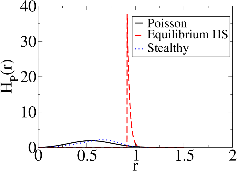
(b)

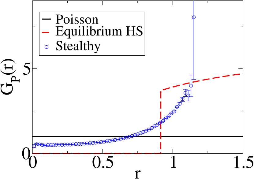
(c)

Figure S2: The particle nearest-neighbor functions $E_{P}(r)$, $H_{P}(r)$, and $G_{P}(r)$ for a Poisson point process at $\rho=1$, an equilibrium hard-sphere system at $\rho=1$ and $\phi=0.4$, and a stealthy ensemble at $\rho=1$ and $\chi\approx 0.10$. The Poisson results were computed with an exact formula [4], the hard-sphere system was computed with an accurate approximation based on the Carnahan-Starling formula [3], and details concerning the stealthy ensemble can be found in the Appendix of the main article. (a) and (b) We can see that the equilibrium hard sphere process has sharply localized nearest-neighbor statistics. (c) The presence of a bounded hole size for the stealthy ensemble can be clearly seen in the divergence of $G_{P}(r)$.

Appendix B Pair Statistics of Stealthy Hyperuniform Point Processes

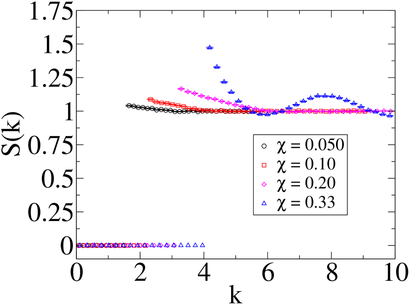
(a)

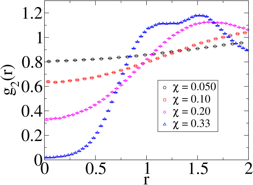
(b)

Figure S3: A comparison of (a) $S(k)$ and (b) $g_{2}(r)$ for simulated 2D stealthy systems at $\rho=1$ and a variety of $\chi$. See the Appendix of the main article for the simulation details of the systems shown.

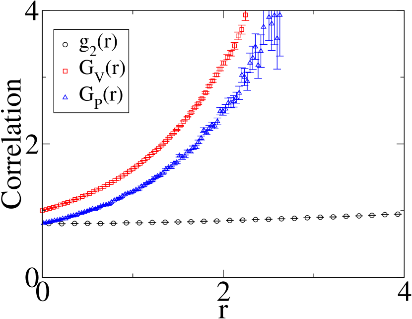
(a)

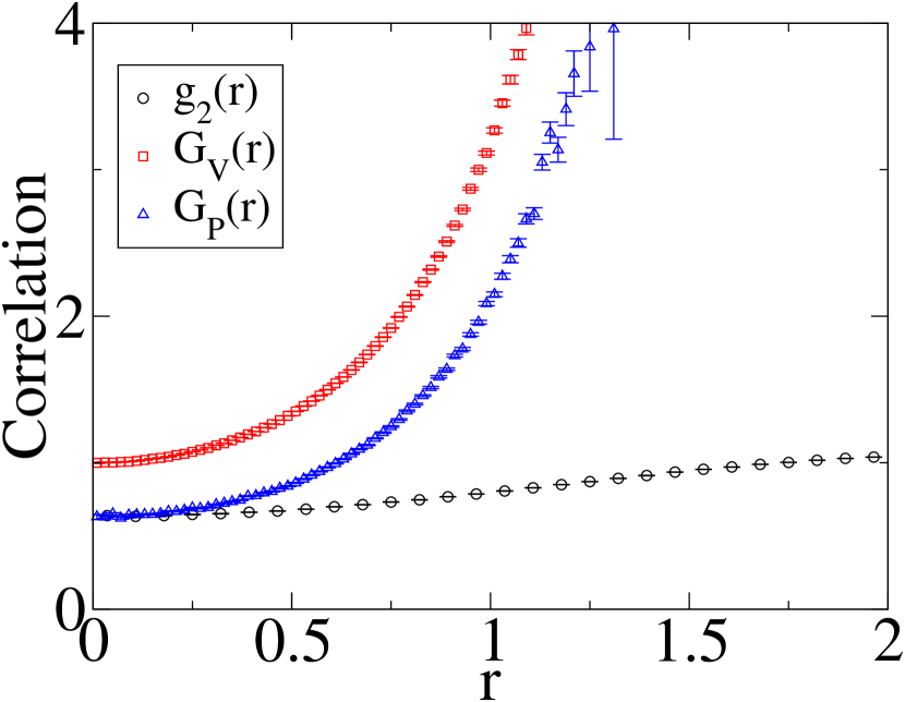
(b)

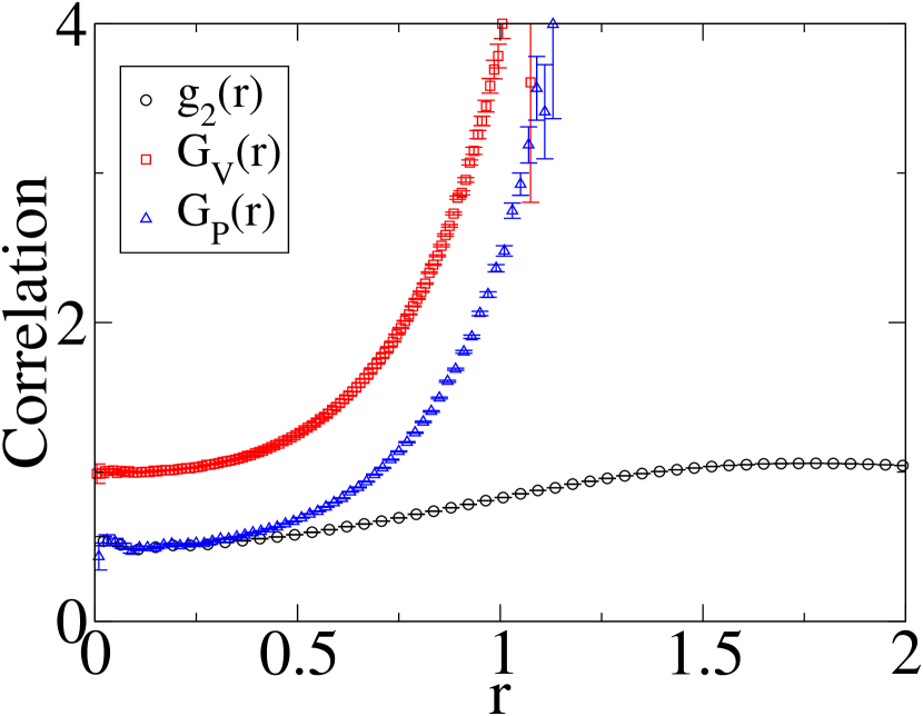
(c)

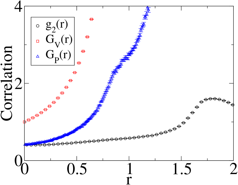
(d)

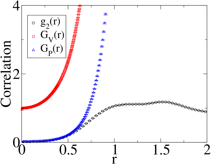
(e)

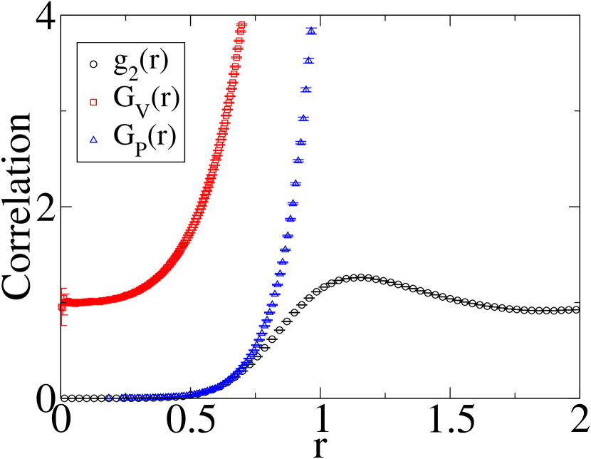
(f)

Figure S4: A comparison of the correlation functions $g_{2}(r)$, $G_{V}(r)$, and $G_{P}(r)$ for a variety of stealthy systems. (a-c) Comparisons for $\chi\approx 0.10$ (see Appendix of main article for details) for one, two, and three dimensions, respectively. (d-f) Comparisons for $\chi\approx 0.33$ (see Appendix of main article for details) for one, two, and three dimensions, respectively.

In this section, we investigate the pair statistics (the pair correlation function $g_{2}(r)$ and the structure factor $S(k)$) of stealthy systems. While theoretical expressions and simulation data on these two correlation functions have previously been reported in Refs. [5] and [6], we make several observations of key interest in the main article. In Fig. S3 below, we show $S(k)$ and $g_{2}(r)$ for 2D stealthy system at various $\chi$. One sees that as $\chi$ is increased, the maximum constrained wavevector $K$ for which $S(k)=0$ increases, and one has an increase in short-range order in the form of stronger low-$r$ correlations in $g_{2}(r)$. In Fig. S4 of the Supplementary Material, we compare $G_{V}(r)$ and $G_{P}(r)$ to the pair correlation function $g_{2}(r)$. In the case of hard sphere systems, these functions are directly related at contact [3]. While no simple relation exists in the case of stealthy systems, one can still observe a number of useful generalities. One finds that for stealthy systems, there exists good numerical evidence for the conjecture $G_{V}(r)\geq G_{P}(r)\geq g_{2}(r)$, at least for small enough $r$. One can also see that while $g_{2}(r)$ and $G_{P}(r)$ tend to the same value as $r\to 0$, $G_{V}(r)$ always tends to unity.

References

References

- [1] Torquato S 2018 Phys. Rep. 745 1–95 ISSN 0370-1573 URL http://www.sciencedirect.com/science/article/pii/S037015731830036X
- [2] Torquato S and Stillinger F H 2003 Phys. Rev. E 68 041113 URL https://link.aps.org/doi/10.1103/PhysRevE.68.041113
- [3] Zhang G, Stillinger F H and Torquato S 2016 Sci. Rep. 6 1–12 ISSN 2045-2322 URL https://www.nature.com/articles/srep36963
- [4] Batten R D, Stillinger F H and Torquato S 2008 J. Appl. Phys. 104 033504 ISSN 0021-8979 URL https://aip.scitation.org/doi/10.1063/1.2961314
- [5] Zhang G, Stillinger F H and Torquato S 2017 Soft Matter 13 6197–6207 URL https://pubs.rsc.org/en/content/articlelanding/2017/sm/c7sm01028a
- [6] Florescu M, Torquato S and Steinhardt P J 2009 PNAS 106 20658–20663 ISSN 0027-8424, 1091-6490 URL https://www.pnas.org/content/106/49/20658
- [7] Man W, Florescu M, Matsuyama K, Yadak P, Nahal G, Hashemizad S, Williamson E, Steinhardt P, Torquato S and Chaikin P 2013 Opt. Express 21 19972–19981 ISSN 1094-4087 URL https://www.osapublishing.org/oe/abstract.cfm?uri=oe-21-17-19972
- [8] Man W, Florescu M, Williamson E P, He Y, Hashemizad S R, Leung B Y C, Liner D R, Torquato S, Chaikin P M and Steinhardt P J 2013 PNAS 110 15886–15891 ISSN 0027-8424, 1091-6490 URL https://www.pnas.org/content/110/40/15886
- [9] Florescu M, Steinhardt P J and Torquato S 2013 Phys. Rev. B 87 165116 URL https://link.aps.org/doi/10.1103/PhysRevB.87.165116
- [10] Froufe-Pérez L S, Engel M, Sáenz J J and Scheffold F 2017 PNAS 114 9570–9574 ISSN 0027-8424, 1091-6490 URL https://www.pnas.org/content/114/36/9570
- [11] Milošević M M, Man W, Nahal G, Steinhardt P J, Torquato S, Chaikin P M, Amoah T, Yu B, Mullen R A and Florescu M 2019 Sci. Rep. 9 1–11 ISSN 2045-2322 URL https://www.nature.com/articles/s41598-019-56692-5
- [12] Zhang G, Stillinger F H and Torquato S 2016 J. Chem. Phys. 145 244109 ISSN 0021-9606 URL https://aip.scitation.org/doi/10.1063/1.4972862
- [13] Torquato S and Chen D 2018 Multifunct. Mater. 1 015001 ISSN 2399-7532 URL https://doi.org/10.1088%2F2399-7532%2Faaca91
- [14] Batten R D, Stillinger F H and Torquato S 2009 Phys. Rev. Lett. 103 050602 URL https://link.aps.org/doi/10.1103/PhysRevLett.103.050602
- [15] Batten R D, Stillinger F H and Torquato S 2009 Phys. Rev. E 80 031105 URL https://link.aps.org/doi/10.1103/PhysRevE.80.031105
- [16] Hansen J P and McDonald I R 1986 Theory of Simple Liquids 2nd ed (London: Academic Press) URL https://www.elsevier.com/books/theory-of-simple-liquids/hansen/978-0-08-057101-0
- [17] Zachary C E and Torquato S 2009 J. Stat. Mech. 2009 P12015 ISSN 1742-5468 URL https://doi.org/10.1088%2F1742-5468%2F2009%2F12%2Fp12015
- [18] Oğuz E C, Socolar J E S, Steinhardt P J and Torquato S 2017 Phys. Rev. B 95 054119 URL https://link.aps.org/doi/10.1103/PhysRevB.95.054119
- [19] Lin C, Steinhardt P J and Torquato S 2017 J. Phys.: Condens. Matter 29 204003 ISSN 0953-8984 URL https://doi.org/10.1088%2F1361-648x%2Faa6944
- [20] Jiao Y, Lau T, Hatzikirou H, Meyer-Hermann M, Corbo J C and Torquato S 2014 Phys. Rev. E 89 022721 URL https://link.aps.org/doi/10.1103/PhysRevE.89.022721
- [21] Donev A, Stillinger F H and Torquato S 2005 Phys. Rev. Lett. 95 090604 URL https://link.aps.org/doi/10.1103/PhysRevLett.95.090604
- [22] Zachary C E, Jiao Y and Torquato S 2011 Phys. Rev. Lett. 106 178001 URL https://link.aps.org/doi/10.1103/PhysRevLett.106.178001
- [23] Jiao Y and Torquato S 2011 Phys. Rev. E 84 041309 URL https://link.aps.org/doi/10.1103/PhysRevE.84.041309
- [24] Chen D, Jiao Y and Torquato S 2014 J. Phys. Chem. B 118 7981–7992 ISSN 1520-6106 URL https://doi.org/10.1021/jp5010133
- [25] Berthier L, Chaudhuri P, Coulais C, Dauchot O and Sollich P 2011 Phys. Rev. Lett. 106 120601 URL https://link.aps.org/doi/10.1103/PhysRevLett.106.120601
- [26] Kurita R and Weeks E R 2011 Phys. Rev. E 84 030401 URL https://link.aps.org/doi/10.1103/PhysRevE.84.030401
- [27] Peebles P J E 1993 Principles of Physical Cosmology (Princeton: Princeton University Press) URL http://adsabs.harvard.edu/abs/1993ppc..book.....P
- [28] Gabrielli A, Sylos Labini F, Joyce M and Pietronero L 2005 Statistical Physics for Cosmic Structures (Berlin Heidelberg: Springer-Verlag) ISBN 978-3-540-40745-4 URL https://www.springer.com/gp/book/9783540407454
- [29] Gabrielli A, Joyce M and Sylos Labini F 2002 Phys. Rev. D 65 083523 URL https://link.aps.org/doi/10.1103/PhysRevD.65.083523
- [30] Gabrielli A, Jancovici B, Joyce M, Lebowitz J L, Pietronero L and Sylos Labini F 2003 Phys. Rev. D 67 043506 URL https://link.aps.org/doi/10.1103/PhysRevD.67.043506
- [31] Torquato S, Scardicchio A and Zachary C E 2008 J. Stat. Mech. 2008 P11019 ISSN 1742-5468 URL https://doi.org/10.1088%2F1742-5468%2F2008%2F11%2Fp11019
- [32] Scardicchio A, Zachary C E and Torquato S 2009 Phys. Rev. E 79 041108 URL https://link.aps.org/doi/10.1103/PhysRevE.79.041108
- [33] Feynman R P and Cohen M 1956 Phys. Rev. 102 1189–1204 URL https://link.aps.org/doi/10.1103/PhysRev.102.1189
- [34] Reatto L and Chester G V 1967 Phys. Rev. 155 88–100 URL https://link.aps.org/doi/10.1103/PhysRev.155.88
- [35] Ghosh S and Lebowitz J L 2018 Commun. Math. Phys. 363 97–110 ISSN 1432-0916 URL https://doi.org/10.1007/s00220-018-3226-5
- [36] Uche O U, Stillinger F H and Torquato S 2004 Phys. Rev. E 70 046122 URL https://link.aps.org/doi/10.1103/PhysRevE.70.046122
- [37] Torquato S, Zhang G and Stillinger F H 2015 Phys. Rev. X 5 021020 URL https://link.aps.org/doi/10.1103/PhysRevX.5.021020
- [38] Fan Y, Percus J K, Stillinger D K and Stillinger F H 1991 Phys. Rev. A 44 2394–2402 URL https://link.aps.org/doi/10.1103/PhysRevA.44.2394
- [39] Uche O U, Torquato S and Stillinger F H 2006 Phys. Rev. E 74 031104 URL https://link.aps.org/doi/10.1103/PhysRevE.74.031104
- [40] Sütő A 2005 Phys. Rev. Lett. 95 265501 URL https://link.aps.org/doi/10.1103/PhysRevLett.95.265501
- [41] Zhang G, Stillinger F H and Torquato S 2015 Phys. Rev. E 92 022119 URL https://link.aps.org/doi/10.1103/PhysRevE.92.022119
- [42] Zhang G, Stillinger F H and Torquato S 2015 Phys. Rev. E 92 022120 URL https://link.aps.org/doi/10.1103/PhysRevE.92.022120
- [43] Torquato S, Lu B and Rubinstein J 1990 J. Phys. A: Math. Gen. 23 L103–L107 ISSN 0305-4470 URL https://doi.org/10.1088%2F0305-4470%2F23%2F3%2F005
- [44] Torquato S, Lu B and Rubinstein J 1990 Phys. Rev. A 41 2059–2075 URL https://link.aps.org/doi/10.1103/PhysRevA.41.2059
- [45] Mehta M L 1991 Random Matrices 2nd ed (San Diego: Academic Press) URL https://www.elsevier.com/books/random-matrices/lal-mehta/978-0-12-488051-1
- [46] Rintoul M D, Torquato S and Tarjus G 1996 Phys. Rev. E 53 450–457 URL https://link.aps.org/doi/10.1103/PhysRevE.53.450
- [47] Reiss H, Frisch H L and Lebowitz J L 1959 J. Chem. Phys. 31 369–380 ISSN 0021-9606 URL https://aip.scitation.org/doi/10.1063/1.1730361
- [48] Torquato S and Lee S B 1990 Physica A 167 361–383 ISSN 0378-4371 URL http://www.sciencedirect.com/science/article/pii/0378437190901218
- [49] Torquato S 1995 Phys. Rev. Lett. 74 2156–2159 URL https://link.aps.org/doi/10.1103/PhysRevLett.74.2156
- [50] Torquato S 1995 Phys. Rev. E 51 3170–3182 URL https://link.aps.org/doi/10.1103/PhysRevE.51.3170
- [51] Finney J L and Bernal J D 1970 Proc. R. Soc. Lond. A 319 479–493 URL https://royalsocietypublishing.org/doi/10.1098/rspa.1970.0189
- [52] Berryman J G 1983 Phys. Rev. A 27 1053–1061 URL https://link.aps.org/doi/10.1103/PhysRevA.27.1053
- [53] Zachary C E and Torquato S 2011 Phys. Rev. E 83 051133 URL https://link.aps.org/doi/10.1103/PhysRevE.83.051133
- [54] Zachary C E, Jiao Y and Torquato S 2011 Phys. Rev. E 83 051308 URL https://link.aps.org/doi/10.1103/PhysRevE.83.051308
- [55] Rintoul M D and Torquato S 1995 Phys. Rev. E 52 2635–2643 URL https://link.aps.org/doi/10.1103/PhysRevE.52.2635
- [56] Sastry S, Corti D S, Debenedetti P G and Stillinger F H 1997 Phys. Rev. E 56 5524–5532 URL https://link.aps.org/doi/10.1103/PhysRevE.56.5524
- [57] Maiti M, Lakshminarayanan A and Sastry S 2013 Eur. Phys. J. E 36 5 ISSN 1292-895X URL https://doi.org/10.1140/epje/i2013-13005-4
- [58] Klatt M A and Torquato S 2016 Phys. Rev. E 94 022152 URL https://link.aps.org/doi/10.1103/PhysRevE.94.022152
- [59] Viot P, Van Tassel P R and Talbot J 1998 Phys. Rev. E 57 1661–1667 URL https://link.aps.org/doi/10.1103/PhysRevE.57.1661
- [60] Macdonald J R 1992 Phys. Rev. A 46 R2988–R2991 URL https://link.aps.org/doi/10.1103/PhysRevA.46.R2988
- [61] Chandrasekhar S 1943 Rev. Mod. Phys. 15 1–89 URL https://link.aps.org/doi/10.1103/RevModPhys.15.1
- [62] Cornell B A, Middlehurst J and Parker N S 1981 J. Colloid Interface Sci. 81 280–282 ISSN 0021-9797 URL http://www.sciencedirect.com/science/article/pii/0021979781903234
- [63] Larcher M and Jenkins J T 2013 Phys. Fluids 25 113301 URL https://aip.scitation.org/doi/10.1063/1.4830115
- [64] Torquato S 2010 Phys. Rev. E 82 056109 URL https://link.aps.org/doi/10.1103/PhysRevE.82.056109
- [65] Torquato S 2002 Random Heterogeneous Materials: Microstructure and Macroscopic Properties Interdisciplinary Applied Mathematics (New York: Springer-Verlag) ISBN 978-0-387-95167-6 URL https://www.springer.com/gp/book/9780387951676
- [66] Sorichetti V, Hugouvieux V and Kob W 2020 Macromolecules 53 2568–2581 ISSN 0024-9297 URL https://doi.org/10.1021/acs.macromol.9b02166
- [67] Keller J B, Rubenfeld L A and Molyneux J E 1967 J. Fluid Mech. 30 97–125 ISSN 1469-7645, 0022-1120 URL https://www.cambridge.org/core/journals/journal-of-fluid-mechanics/article/extremum-principles-for-slow-viscous-flows-with-applications-to-suspensions/1EE0F34489BFB29E304AD1E4DA6D4D4E
- [68] Rubinstein J and Torquato S 1988 J. Chem. Phys. 88 6372–6380 ISSN 0021-9606 URL https://aip.scitation.org/doi/abs/10.1063/1.454474
- [69] Torquato S and Rubinstein J 1989 J. Chem. Phys. 90 1644–1647 ISSN 0021-9606 URL https://aip.scitation.org/doi/10.1063/1.456655
- [70] Torquato S, Uche O U and Stillinger F H 2006 Phys. Rev. E 74 061308 URL https://link.aps.org/doi/10.1103/PhysRevE.74.061308
- [71] Zhang G and Torquato S 2013 Phys. Rev. E 88 053312 URL https://link.aps.org/doi/10.1103/PhysRevE.88.053312
- [72] Torquato S 1986 J. Stat. Phys. 45 843–873 ISSN 1572-9613 URL https://doi.org/10.1007/BF01020577
- [73] Hertz P 1909 Math. Ann. 67 387–398 ISSN 1432-1807 URL https://doi.org/10.1007/BF01450410
- [74] Middlemas T M and Torquato S Supplementary Material
- [75] Daley D J and Vere-Jones D 1998 An Introduction to the Theory of Point Processes Springer Series in Statistics (New York: Springer-Verlag) ISBN 978-1-4757-2001-3 URL https://www.springer.com/gp/book/9781475720013
- [76] Chiu S N, Stoyan D, Kendall W S and Mecke J 2013 Stochastic Geometry and Its Applications 3rd ed URL https://www.wiley.com/en-us/Stochastic+Geometry+and+Its+Applications%2C+3rd+Edition-p-9780470664810
- [77] Hoover W G, Hoover N E and Hanson K 1979 J. Chem. Phys. 70 1837–1844 ISSN 0021-9606 URL https://aip.scitation.org/doi/10.1063/1.437660
- [78] Speedy R J and Reiss H 1991 Mol. Phys. 72 1015–1033 ISSN 0026-8976 URL https://doi.org/10.1080/00268979100100751
- [79] Conway J and Sloane N J A 1999 Sphere Packings, Lattices and Groups 3rd ed Grundlehren der mathematischen Wissenschaften (New York: Springer-Verlag) ISBN 978-0-387-98585-5 URL https://www.springer.com/gp/book/9780387985855
- [80] Torquato S and Stillinger F H 2006 Experiment. Math. 15 307–332 ISSN 1058-6458, 1944-950X URL https://projecteuclid.org/euclid.em/1175789761
- [81] Baus M and Colot J L 1987 Phys. Rev. A 36 3912–3925 URL https://link.aps.org/doi/10.1103/PhysRevA.36.3912
- [82] Kim J and Torquato S 2018 Phys. Rev. B 97 054105 URL https://link.aps.org/doi/10.1103/PhysRevB.97.054105
- [83] Grinstead C M and Snell J L 1997 Introduction to Probability 2nd ed (Providence: American Mathematical Society)
- [84] Hunter J 2004 Applied Asymptotic Analysis: Math 204 Lecture Notes
- [85] Feldman J 2008 Taylor Series and Asymptotic Expansions
- [86] Frenkel D and Smit B 2002 Understanding Molecular Simulation: From Algorithms to Applications 2nd ed (San Diego: Academic Press) URL https://www.elsevier.com/books/understanding-molecular-simulation/frenkel/978-0-12-267351-1

References

- [1] Zhang G, Stillinger F H and Torquato S 2017 Soft Matter 13 6197–6207 URL https://pubs.rsc.org/en/content/articlelanding/2017/sm/c7sm01028a
- [2] Ghosh S and Lebowitz J L 2018 Commun. Math. Phys. 363 97–110 ISSN 1432-0916 URL https://doi.org/10.1007/s00220-018-3226-5
- [3] Torquato S, Lu B and Rubinstein J 1990 Phys. Rev. A 41 2059–2075 URL https://link.aps.org/doi/10.1103/PhysRevA.41.2059
- [4] Hertz P 1909 Math. Ann. 67 387–398 ISSN 1432-1807 URL https://doi.org/10.1007/BF01450410
- [5] Torquato S, Zhang G and Stillinger F H 2015 Phys. Rev. X 5 021020 URL https://link.aps.org/doi/10.1103/PhysRevX.5.021020
- [6] Zhang G, Stillinger F H and Torquato S 2015 Phys. Rev. E 92 022119 URL https://link.aps.org/doi/10.1103/PhysRevE.92.022119