A consistent and robust measurement of the thermal state of the IGM at from a large sample of Ly forest spectra: Evidence for late and rapid HeII reionization
Abstract
We characterise the thermal state of the intergalactic medium (IGM) in ten redshift bins in the range with a sample of 103 high resolution, high S/N Ly forest spectra using four different flux distribution statistics. Our measurements are calibrated with mock spectra from a large suite of hydrodynamical simulations post-processed with our thermal IGM evolution code cite, finely sampling amplitude and slope of the expected temperature-density relation. The thermal parameters inferred from our measurements of the flux power spectrum, Doppler parameter distribution, as well as wavelet and curvature statistics agree well within their respective errors and all clearly show the peak in temperature and minimum in slope of the temperature density relation expected from He ii reionization. Combining our measurements from the different flux statistics gives K for the peak temperature at mean density and a corresponding minimum slope . The peak in the temperature evolution occurs around , in agreement with previous measurements that had suggested the presence of such a peak, albeit with a large scatter. Using cite, we also calculate the thermal state of the IGM predicted by five widely used (spatially homogeneous) UV-background models. The rather rapid thermal evolution inferred by our measurements is well reproduced by two of the models, if we assume (physically well motivated) non-equilibrium evolution with photo-heating rates that are reduced by a moderate factor of . The other three models predict He ii reionization to be more extended with a higher temperature peak occurring somewhat earlier than our measurements suggest.
keywords:
cosmology: large-scale structure of Universe - methods: numerical - galaxies: intergalactic medium - QSOs: absorption lines1 Introduction
Ly absorption seen in the spectra of distant bright QSOs (Quasi Stellar Objects) allow one to probe the thermal and ionization history of the Intergalactic Medium (IGM) in addition to constraining cosmological parameters. The thermal state of the IGM is often characterized by normalization and slope of the temperature-density relation (TDR, ; Hui & Gnedin, 1997), while the ionization state of the IGM is characterized by H i and He ii photo-ionization rates (e.g. Haardt & Madau, 1996). These parameters have been measured using high-resolution, high signal-to-noise spectroscopic observations in conjunction with high-resolution hydrodynamical simulations.
Accurate measurements of thermal parameters and photo-ionization rates of the IGM have been used to place constraints on (i) the epoch and extent of H i and He ii reionization (Miralda-Escudé & Rees, 1994; Theuns et al., 2002b; Worseck et al., 2011; Puchwein et al., 2015; Worseck et al., 2016; Upton Sanderbeck et al., 2016; Gaikwad et al., 2019; Worseck et al., 2019; Upton Sanderbeck & Bird, 2020), (ii) ionizing ultra-violet background (UVB) models that are important inputs for cosmological hydrodynamical simulations (McDonald & Miralda-Escudé, 2001; Bolton et al., 2005; Faucher-Giguère et al., 2009; Haardt & Madau, 2012; Khaire & Srianand, 2015; Oñorbe et al., 2017; Khaire & Srianand, 2019; Puchwein et al., 2019; Faucher-Giguère, 2020, hereafter \al@haardt2012,khaire2015a,onorbe2017,khaire2019a,puchwein2019,faucher2020; \al@haardt2012,khaire2015a,onorbe2017,khaire2019a,puchwein2019,faucher2020; \al@haardt2012,khaire2015a,onorbe2017,khaire2019a,puchwein2019,faucher2020; \al@haardt2012,khaire2015a,onorbe2017,khaire2019a,puchwein2019,faucher2020; \al@haardt2012,khaire2015a,onorbe2017,khaire2019a,puchwein2019,faucher2020; \al@haardt2012,khaire2015a,onorbe2017,khaire2019a,puchwein2019,faucher2020 respectively), (iii) the escape fraction of H i ionizing photons from galaxies and the relative contribution of galaxies and QSOs to the total H i ionizing background (Faucher-Giguère et al., 2008; Khaire et al., 2016; Khaire, 2017), (iv) and the effect of non-radiative processes like heating by cosmic rays (Nath & Biermann, 1993; Samui et al., 2005), blazars (Chang et al., 2012; Puchwein et al., 2012) and dark matter annihilation (Cirelli et al., 2009; Liu et al., 2020).
He ii reionization is expected to be completed in the redshift range . He ii reionization injects energy into the IGM and thereby broadens the absorption features (Schaye et al., 2000), decreases the neutral fraction of hydrogen (Rauch et al., 1997; Bolton & Haehnelt, 2007) and leads to additional pressure smoothing of the density and flux fields (Gnedin & Hui, 1998; Peeples et al., 2010). Accurate measurements of thermal parameters in this redshift range can therefore provide important constraints on the models of He ii reionization.
The thermal parameters of the IGM have been measured by (i) decomposing absorption features into multi-component Voigt profiles and identifying the lower envelope of the line width (b-parameter) vs H i column density ( ; Schaye et al., 1999, 2000; Bolton et al., 2014; Hiss et al., 2018; Telikova et al., 2019), (ii) measuring the small scale suppression in the transmitted flux power spectrum (Theuns et al., 2000; McDonald, 2003; Kim et al., 2004; Walther et al., 2019; Boera et al., 2019), (iii) using curvature (defined as, where and are the first and second derivatives of the normalised flux with respect to the wavelength) statistics (Becker et al., 2011; Boera et al., 2014; Padmanabhan et al., 2015) or (iv) characterising Fourier modes of the flux distribution in the range sensitive to thermal parameters using wavelet analysis (Zaldarriaga, 2002; Theuns et al., 2002a; Lidz et al., 2010; Garzilli et al., 2012). Even if the same observational data is used, the sensitivity to small changes in thermal parameters and associated systematic uncertainties are found to be different for different flux statistics (see §5 for a detailed discussion of this). Ideally, one would thus like to calculate all these different flux statistics simultaneously and consistently for the same data set to obtain joint best fit values of the thermal parameters and the associated errors. In order to obtain robust and consistent results it is also important to perform such an analysis using a consistent set of model parameters.
As simulated data are an integral part of the parameter estimation from Ly forest data, the reliability and accuracy of the extracted parameters depend on the assumptions involved in the simulations and the ability to perform a wide range of simulations that span a sufficiently wide parameter space with good i.e. not too coarse sampling. Generating such a set of simulations accounting for the relevant physical effects is challenging. At any given epoch the pressure smoothing of the density field depends on the past thermal history (Gnedin & Hui, 1998; Peeples et al., 2010; Kulkarni et al., 2015; Nasir et al., 2016; Rorai et al., 2017a) and one needs self-consistent high-resolution cosmological hydrodynamical simulations of the IGM (Springel, 2005; Almgren et al., 2013; Bolton et al., 2017). Practically one achieves a range of and in simulations by varying photo-heating rates of H i and He ii as a function of redshift (see for example, Schaye et al., 2000; Becker et al., 2011). Such simulations are computationally expensive which limits the thermal parameter space that can be probed at any given redshift.
As noted before, most simulations used for this purpose are performed assuming a uniform ionizing background and ionization equilibrium. While these are good approximations after He ii reionization is complete such simulations do not capture all relevant physics before and during He ii reionization, i.e., (see Puchwein et al., 2015, 2019; Gaikwad et al., 2019). For this one needs simulations that also account for the non-equilibrium effects during He ii reionization. Ideally one would also like simulations to incorporate the spatially inhomogeneous nature of He ii reionization and the corresponding fluctuations of the UV background. However, such simulations will not only require to include radiative transfer, but also large box sizes as well as high resolution and thus very high dynamic range to capture the relevant physical processes accurately.
The main aim of this work is to obtain a consistent measurement of thermal parameters using the larger data sets that have become publicly available recently. Thanks to compilations like kodiaq dr2 (O’Meara et al., 2015, 2017, from KECK/HIRES archival data) and UVES squad dr1 (Murphy et al., 2019, from VLT/UVES archival data), large samples of QSO spectra with high resolution ( km s-1 adequate to resolve the thermally broadened Ly absorption lines) and high S/N are now available for analysis. These samples have dramatically increased the number of available QSO spectra that have been reduced and continuum normalised using uniform techniques.
Additional impetus to perform a consistent measurement of thermal parameters for these large samples comes from two tools we have developed over the past few years: (i) the Code for Ionization and Temperature Evolution (cite, Gaikwad et al., 2017a) and (ii) the VoIgt profile Parameter Estimation Routine (viper, Gaikwad et al., 2017b), an automatic Voigt profile fitting code that decomposes Ly absorption spectra into Voigt profile components. cite not only allows us to construct models with a wide range of thermal and ionization histories efficiently without running full hydrodynamical simulations, but also enables us to calculate the non-equilibrium evolution of the thermal and ionization state of the gas (see Gaikwad et al., 2019, for details). cite has been shown to reproduce the results of full hydro-simulations to well within 10 percent accuracy (Gaikwad et al., 2018). viper runs on parallel architectures and allows us to perform a Voigt profile analysis for large samples of observed and simulated spectra consistently (see Maitra et al., 2019, 2020, for a clustering analysis using Voigt profile components). Thanks to these two codes, we are in a position to measure the physical parameters of the IGM from Ly forest data by simultaneously using the different statistics mentioned above.
We present here the measurements of thermal parameters ( and ) over the redshift range in 10 redshift bins of width using 103 high resolution, high S/N QSO spectra drawn from the kodiaq dr2 sample. The paper is organized as follows, in §2 we present the details of the observational data used in this work and compare our new measurements of the mean flux as a function of redshift, H i column density distribution, flux PDF and power-spectrum with measurements in the literature. We describe our simulations and explain how we generate simulated spectra for a wide range of finely spaced thermal parameters in §3. We provide details of four different flux statistics of Ly forest used to measure thermal parameters in §4 and in online supplementary appendix E. In §5 we show our measurements of thermal parameters, present our error analysis and compare our measurements with measurements in the literature. In §6 we show predictions for the thermal parameter evolution for different UVB models. Finally we summarize in §7. Note that we make all the measurements from observational data available to the community as online supplementary material.
The default cosmological parameters used here are , consistent with a flat CDM cosmology (Planck Collaboration et al., 2014). All distances are given in comoving units unless specified. We have expressed in units of denoted by . We often refer to as thermal parameters in this work.
2 Observations
| Median SNR | |||
|---|---|---|---|
| 32 | 14.7 | ||
| 37 | 21.2 | ||
| 33 | 19.2 | ||
| 26 | 19.3 | ||
| 28 | 19.7 | ||
| 26 | 23.4 | ||
| 16 | 22.0 | ||
| 12 | 22.4 | ||
| 5 | 22.8 | ||
| 7 | 22.3 |
We use observed spectra from the second data release of the Keck Observatory Database of Ionized Absorption toward Quasars (kodiaq dr2) survey (O’Meara et al., 2015, 2017)111https://www2.keck.hawaii.edu/koa/public/koa.php. The sample consists of 300 QSO spectra with emission redshifts . All available spectra are continuum normalised and the data product provides normalised flux and the associated error as a function of wavelength. Many of these QSOs were observed more than once with different exposure times. We co-added all the spectra using the procedure described in online supplementary appendix A.
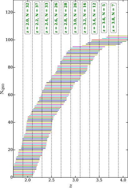
In total there are 214 QSO spectra that cover the Ly forest in the range . We manually checked all the coadded spectra and excluded spectra if one or more of the following criteria are satisfied: (i) sightline does not (partially or fully) contain Ly forest in the redshift range , (ii) sightline contains Damped Ly (DLA) or sub-DLA systems, (iii) the sightline contains large spectral gaps (see online supplementary appendix A for details), or (iv) the median S/N per pixel along the sightlines is smaller than . After excluding the QSO spectra with above criteria, the resulting sample consists of 103 QSO spectra. Fig. 1 shows the Ly redshift range corresponding to the wavelength range between the Ly and Ly emission lines of the 103 QSOs in our sample. The Ly absorption close to the QSOs is expected to be influenced by the enhanced ionizing flux due to the QSOs (Carswell et al., 1982; Kulkarni & Fall, 1993; Srianand & Khare, 1996; Lidz et al., 2007; Calverley et al., 2011; Bolton et al., 2012). We exclude such biased QSO proximity regions (i.e 10 pMpc from the QSO towards us) in our subsequent analysis. This choice of QSO proximity region size corresponds to the quasar rest frame wavelength of Å at . To avoid possible contamination from intrinsic O iv absorption we consider only regions with rest wavelength greater than 1050 Å at the quasar emission redshift.
In order to measure the evolution of thermal parameters, we divide our sample into ten redshift bins centered on with a bin width of . Fig. 1 shows the number of QSO spectra contributing to our sample in each of these ten redshift bins. The properties of the observed spectra in these redshift bins are summarized in Table 1. The median S/N of the observed sample is in all redshift bins. The observed Ly forest regions are usually contaminated by metal lines that produce narrow absorption features and potentially could bias our measurements of and . To account for this we manually identified contaminating metal line absorption using the list of known intervening metal line systems along these sightlines. It is not always possible to identify all the metal lines contaminating the Ly forest. However, as we fit all the observed spectra with our automated Voigt profile fitting routine viper (Gaikwad et al., 2017b) we can mitigate this. We treat all lines with km s-1 as metal lines. Finally, we replace all metal lines by continuum and add noise to the replaced regions. We have checked the effect of residual metal line contamination on our measurements and found the effect to be marginal (see online supplementary appendix H).
There could be additional errors in the observed flux due to continuum fitting uncertainties. Continuum fitting uncertainties depend not only on the number of unabsorbed spectral regions used in the fit but also on the observed S/N per pixel in these regions and the QSO spectral energy distribution (SED). Since the true QSO continuum is unknown, an exact quantification of the contribution of continuum fitting uncertainty to the error in the normalised flux is not available for the kodiaq dr2 sample. The continuum fitting uncertainty is expected to be of the order of a few percent for moderate S/N data (O’Meara et al., 2015). We thus allow for the possibility of a systematic error of per cent in the normalised flux for our final and measurements to account for continuum uncertainties.
2.1 Comparison of observed statistics with previous measurements
In this section, we derive the statistics of the transmitted Ly flux for our sample and compare them with results in the literature. In particular, we compare the evolution of mean flux, flux probability distribution function (FPDF), flux power-spectrum (FPS) and H i column density distribution function (CDDF) from our sample with other measurements in the literature. In §4 we describe in detail our method of calculating these flux statistics (along with other statistics) from observations and simulations.
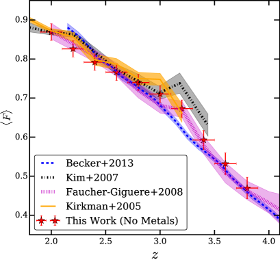
The last column in Table 1 provides the mean observed transmitted flux measured in each redshift bin. The error on the mean flux given also accounts for the systematic uncertainty due to continuum placement. As expected, the mean flux decreases monotonically with redshift due to the increase in the opacity of the IGM at higher redshifts. In Fig. 2, we compare the evolution of the mean flux of our sample (see Table 1) with that from Kirkman et al. (2005); Kim et al. (2007); Faucher-Giguère et al. (2008) and Becker et al. (2013). The evolution in Kirkman et al. (2005); Kim et al. (2007) and Faucher-Giguère et al. (2008) is obtained using high-resolution QSO absorption spectra, while Becker et al. (2013) obtained their evolution using very large number of SDSS spectra that have lower resolution and low SNR compared to the typical high-resolution data used in the literature and our work here.
Our evolution is broadly consistent with Kirkman et al. (2005); Kim et al. (2007); Faucher-Giguère et al. (2008); Becker et al. (2013) with some notable differences. at and in our sample is smaller by than that of Kirkman et al. (2005); Kim et al. (2007). One possible reason could be the number of QSO lines of sight used in their work, at those redshifts. Our measurement at ( ) is systematically larger (smaller) than that of Becker et al. (2013). The evolution in our sample is in good agreement with that from Faucher-Giguère et al. (2008) over the full redshift range. We see a slight enhancement in at in the kodiaq dr2 sample (see online supplementary appendix B for more details). We have also analyzed the squad dr1 QSO sample for the purpose of calculating the evolution (Murphy et al., 2019). The evolution from two samples are in good agreement (within ) with each other (except at . We find that the enhancement in at is less prominent in squad dr1, but the evolution shows a change in slope at . It is noteworthy that the statistics sensitive to thermal parameters are in good agreement with each other for the kodiaq dr2 and squad dr1 samples. Furthermore, note again that we rescale simulated optical depths to match the observed which reduces the effect of differences in on thermal parameters. The presence or absence of the slight excess of discussed above has thus only a marginal effect on measurements of presented in this work.
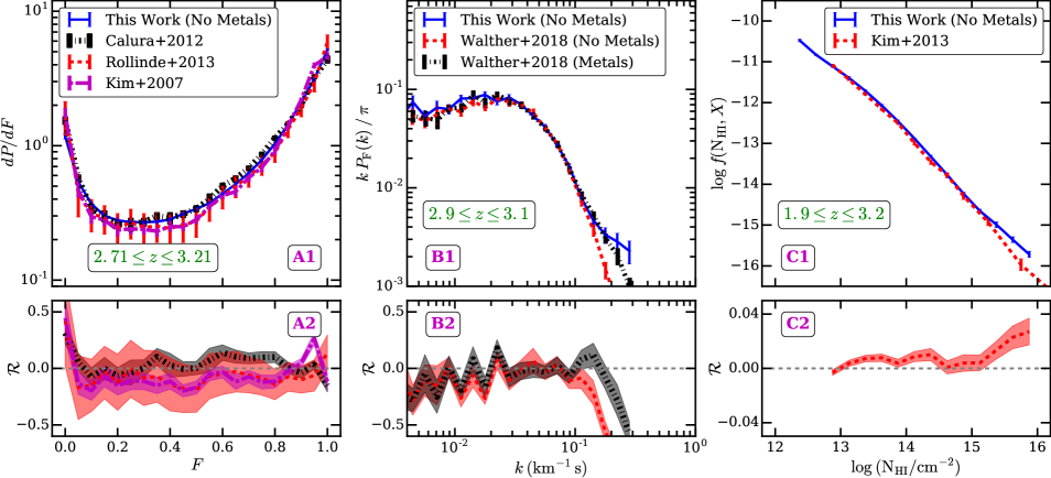
We compare the FPDF at from our sample with those from Kim et al. (2007); Calura et al. (2012); Rollinde et al. (2013) in Fig. 3 (panel A1 and A2). The number of spectra used by Calura et al. (2012); Rollinde et al. (2013) and Kim et al. (2007) is 2, 5 and 8 respectively, while our sample contains spectra. Despite this, our FPDF in the range is within percent of that from Kim et al. (2007); Calura et al. (2012); Rollinde et al. (2013). The FPDF statistics appears reasonably well converged even for small number of spectra. In this work, we focus on the FPDF in the flux range because the flux at () could be dominated by sky subtraction (continuum placement) uncertainty.
In panels B1 and B2 of Fig. 3, we show a comparison of the FPS from our sample with that from Walther et al. (2018). Even though the sample used in Walther et al. (2018) and our work here is the same (i.e, the kodiaq DR2 sample), the number of QSOs per redshift bin is different because of our selection criteria (see §2). Our method of calculating the FPS is also different. Since our sample is selected such that the spectra do not contain spectral gaps, we compute the power spectrum using FFT. We also forward model the simulated Ly forest spectra to mimic the noise and instrumental broadening properties of the observed spectra. Hence when calculating the FPS, we neither subtract the noise power nor deconvolve the instrumental broadening. We also replace metal lines with continuum and add noise in the replaced regions, while Walther et al. (2018) mask metal line regions. Despite these differences, when we compare our FPS at with that from Walther et al. (2018), we find good agreement. Note that we use the FPS only at to measure and , as these scales are most sensitive to the variation of thermal parameters.
In Fig. 3 (panel C1-C2), we compare the CDDF from Kim et al. (2013) with that obtained from our sample using viper. For a fair comparison, we restrict the observed spectra of our sample to the redshift range and we use the same definition of the CDDF. Kim et al. (2013) present the CDDF for the range since their sample is incomplete at . We account for the incompleteness in our measurement by calculating the sensitivity curve hence our CDDF measurements are shown from to . Our observed CDDF is in good agreement ( percent) with that of Kim et al. (2013). At , we find more systems compared to Kim et al. (2013). This may be due to the fact that viper fits only Ly absorption while Kim et al. (2013) fit Ly and Ly absorption simultaneously. Despite this, the two CDDF in the range are consistent with each other. We refer the reader to online supplementary appendix C for a discussion of the associated errors in these statistics for our measurements and those in the literature.
3 Simulations
We evolve the cosmological density, velocity and temperature field using the smooth particle hydrodynamic (SPH) gadget-3 222http://wwwmpa.mpa-garching.mpg.de/gadget/ code. The initial conditions are generated at using 2lpt (Scoccimarro et al., 2012)333http://cosmo.nyu.edu/roman/2LPT/. Our fiducial simulations have a box size of cMpc and have baryon particles and an equal number of dark matter particles corresponding to a gas particle mass of . The gravitational softening length is set to ckpc. We found this to be the best compromise in terms of resolution, dynamic range and ability to run a sufficiently fine grid of thermal parameters. We have performed a resolution study using the Sherwood simulation suite 444https://www.nottingham.ac.uk/astronomy/sherwood/ and show that our results are sufficiently well converged for our choice of simulation (see §4.4, Bolton et al., 2017). We also use the Sherwood simulation suite to demonstrate that our measurements are not significantly affected by the somewhat limited box-size and thus spatial dynamical range.
gadget-3 is a modified version of the publicly available gadget-2 code (Springel, 2005) that incorporates the radiative heating and cooling by a time varying, spatially uniform UV background. For our fiducial simulations we incorporate the KS19 UVB model (QSO SED index ) by modifying the TREECOOL file in gadget-3. We store the output of the gadget-3 code at equal redshift intervals . We employ a simplified star formation criteria that converts particles with and into stars (the so called quick Ly option, Viel et al., 2004a) and do not include AGN or stellar feedback.
To generate physically motivated thermal histories one needs to perform computationally expensive cosmological simulations for a range of UVB models (Becker et al., 2011; Walther et al., 2019). In this work, we follow the approach laid out by Gaikwad et al. (2018) and explore the thermal parameter space efficiently. Our procedure to simulate the thermal history is: (i) We perform a gadget-3 simulation with the KS19 UVB model using equilibrium ionization evolution equation. The typical thermal parameters of such a simulation at are K and . (ii) To obtain the variation in thermal parameters, we modify the photo-heating rates in the UVB code (see online supplementary appendix D). We then solve the ionization and thermal evolution equation for each particle on gadget-3 outputs using our thermal evolution code Code for Ionization and Temperature Evolution (cite, Gaikwad et al., 2017a) (iii) We apply pressure smoothing corrections while extracting the and fields along a sightline by convolving the SPH kernel with the pressure smoothing Gaussian kernel (Gaikwad et al., 2018). (iv) Finally, we compute the Ly optical depth accounting for thermal broadening, natural line width broadening and peculiar velocity effects. In Gaikwad et al. (2017a, 2019), we showed that thermal parameters can be constrained within uncertainty provided the mean flux is matched between simulation and observations. However unlike Gaikwad et al. (2019), in this work, we solve for the ionization evolution assuming equilibrium while solving the thermal evolution using the non-equilibrium equations.
We vary the thermal parameter evolution by scaling the H i, He i and He ii photo-heating rates of the KS19 UVB (see Becker et al., 2011, for a similar approach). We generate combinations for a finely sampled grid such that is varied from K to K in steps of 500 K while is varied from to in steps of 0.05 at . The corresponding and values at other redshifts differ by percent. We have thus simulated the Ly forest for different thermal histories. The computational time required to run and extract Ly forest spectra for 999 UVB models is around million cpu hours. One can perform self-consistent L10N512 simulations in similar time. Note that the number of thermal parameters probed in this work is larger by a factor of and than those by Walther et al. (2019, ) and Becker et al. (2011, ), respectively. We refer the reader to online supplementary appendix D for more details.
We generate the overdensity (), neutral fraction ( ), temperature () and peculiar velocity fields along 20000 random skewers through our simulation box at . In each redshift bin we concatenate the fields to match the observed redshift path length (). However, while computing the FPS, we do not concatenate spectra as there is no correlation beyond the length of the simulation box. The Ly optical depth is generated from the , , and fields accounting for Doppler broadening, natural line broadening and peculiar velocity effects (Choudhury et al., 2001; Padmanabhan et al., 2014). For each redshift bin, we construct a single simulated mock sample with the same number of spectra as observed in that redshift bin (see Gaikwad et al., 2017a, for a similar method at ). The simulated spectra in a mock sample mimic the observed spectra by (i) convolving the flux field with Gaussian instrumental broadening (FWHM km s-1) (iii) resampling the pixel distribution similar to the observed data, and (iii) by adding Gaussian random noise generated from the observed S/N per pixel array. We generate 100 such mock samples to constitute a mock suite for each redshift bin. For example, in the redshift range , each mock sample consists of 26 simulated spectra and a mock suite consists of simulated spectra. We use these 100 mock samples to estimate the errors on different flux statistics. In order to compare the simulations with observations, we calculate the flux statistics that we will show to be sensitive to thermal parameters in the next section.
4 Method
The increase in temperature of the IGM due to He ii reionization has the following main effects on the H i Ly forest (i) broadening of the absorption features (Schaye et al., 2000; Lidz et al., 2010; Becker et al., 2011), (ii) decrease in neutral fraction due to the temperature dependence of the recombination rate (Rauch et al., 1997; Bolton & Haehnelt, 2007; Becker & Bolton, 2013; Viel et al., 2017; Khaire et al., 2019) and (iii) pressure smoothing of the density and flux fields (Gnedin & Hui, 1998; Peeples et al., 2010; Kulkarni et al., 2015; Lukić et al., 2015; Rorai et al., 2017a; Maitra et al., 2019). Since increasing the temperature of the IGM leads to smoothing of the flux, the Ly forest statistics used in the past for measuring thermal parameters are based on either extracting small scale features or measuring the broadening of the absorption lines. In what follows, we describe the statistics used in this work to measure and .
4.1 Ly forest statistics
In the literature, and have been measured by two different kind of statistics, namely, those derived from the transmitted Ly flux directly and those derived by fitting the transmitted Ly flux with multi-component Voigt profiles. We use here four statistics, namely, the flux power spectrum (FPS), the wavelet statistics (WS), the curvature statistics (CS) and the line width distribution (hereafter BPDF) of Voigt profile components to measure the thermal parameters.
4.1.1 Flux power spectrum (FPS)
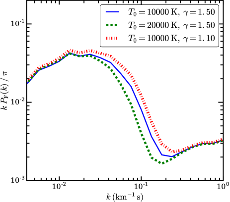
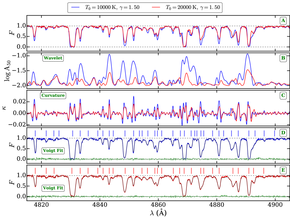
The FPS is sensitive to a wide range of parameters: thermal parameters, , cosmological parameters (), the free-streaming length of dark matter particles and neutrinos etc (Viel et al., 2004b; Garzilli et al., 2017; Iršič et al., 2017a, b; Gaikwad et al., 2017a; Khaire et al., 2019; Gaikwad et al., 2020). For a given set of cosmological parameters in the CDM framework, the FPS is sensitive to small scale smoothing of the Ly flux arising from heating of the IGM. Fig. 4 (panel A) illustrates the effect of increased temperature on the Ly flux. The flux in the higher- model (for brevity, let us call it the hot model) is somewhat smoother and shows less peaked absorption as compared to the lower- (the cold model) model.
To calculate the FPS, we take the Fourier transform of the flux contrast where is the mean flux in a given redshift bin. We bin the Fourier power in logarithmic bins centered on ( km-1 s) and with bin width . This probes scales from km s-1 to km s-1. The lower and upper limits of are motivated by the size of our simulation box and the resolution of the observed spectra, respectively. While computing the FPS, we do not concatenate spectra as there is no correlation beyond the length of the simulation box.
Fig. 5 shows the sensitivity of the FPS to the thermal parameters and . The power at for a model with higher (smaller ) is smaller due to more smoothing of the flux. The model predicted FPS at scales km-1 s are nearly same as the dark matter density field is the same for all models. On the other hand, the FPS at km-1 s is dominated by observational systematic effects such as instrumental broadening and finite S/N per pixel. The FPS at ( ) is clearly sensitive to thermal parameters.
4.1.2 Wavelet Statistics (WS)
Wavelets are wave-like oscillations that are localized in both the real space and frequency domains. One can use a suitable wavelet to extract the scales in transmitted Ly flux that are sensitive to and (Zaldarriaga, 2002; Theuns et al., 2002a; Lidz et al., 2010; Garzilli et al., 2012). Mathematically, this is equivalent to a convolution of the transmitted Ly flux with the wavelets. Throughout this work, we use Morlet wavelets that look like a Gaussian in Fourier space555We have also performed analysis with Mexican hat and Shannon wavelets and found that the results are insensitive to the choice of wavelet.. The oscillation frequency of the wavelet depends on the center of the Gaussian in Fourier space. While the width of the wavelet is related to the width of the Gaussian in Fourier space. The Morlet wavelets have the functional form,
| (1) |
where is velocity, is wavelet scale, is a normalization constant obtained by demanding that wavelets are square integrable i.e., . The wavelet transform of the flux (hereafter the wavelet field ) is the convolution of the wavelet with the transmitted Ly flux (),
| (2) |
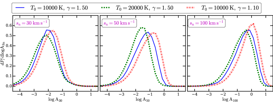
Fig. 4 (panel B) demonstrates the sensitivity of the wavelet amplitude (for the wavelet scale km s-1) to the temperature of the IGM666Wavelet amplitudes can be negative hence we plot logarithm of absolute values of wavelet amplitude.. The wavelet amplitudes () in the hot model are systematically smaller than those from the cold model. It is also evident that the wavelet amplitude picks out small scale variations in the flux field. To quantify the effect of and on the wavelet amplitude, we focus on the probability distribution function of the wavelet field. Usually, the wavelet field needs to be smoothed (e.g., using a boxcar filter of km s-1, see Lidz et al., 2010) to reduce the effect of flux noise on the wavelet PDF. However, we find that such a boxcar smoothing reduces the sensitivity of the wavelet PDF to and . Instead we use kernel density estimation to calculate the wavelet PDF. This reduces the effect of noise while preserving the sensitivity of the wavelet PDF to and (see online supplementary appendix E.1 for details).
Fig. 6 shows the comparison of the wavelet PDF for 3 models (i) K, , (ii) K, , and (iii) K, . The wavelet PDF is systematically shifting to lower values for higher at all the three wavelet scales km s-1. Fig. 6 also shows that the wavelet scale km s-1 is most sensitive to variation in . At smaller wavelet scales km s-1 it is less sensitive to due to observational effects (noise and resolution) while larger wavelet scales km s-1 trace the underlying dark matter density field which is the same for the three models. The wavelet amplitudes are systematically lower for higher values. This is expected because for the same normalization , a higher value corresponds to larger temperature at . Since a significant fraction of the Ly absorption at comes from , the Ly absorption lines in models with higher are expected to be broader. But it is interesting to note that the wavelet scale km s-1 is slightly more sensitive to than to . Thus, if we simultaneously use wavelet PDFs at scales ( km s-1) , the constrains on and should be better than using the wavelet PDF for the individual scales.
4.1.3 Curvature Statistics
The thermal broadening of the absorption lines can also be characterized by the curvature of the absorption features (Becker et al., 2011). The curvature () is essentially a measure of the rate of change of direction of a point that moves on a curve and is defined as
| (3) |
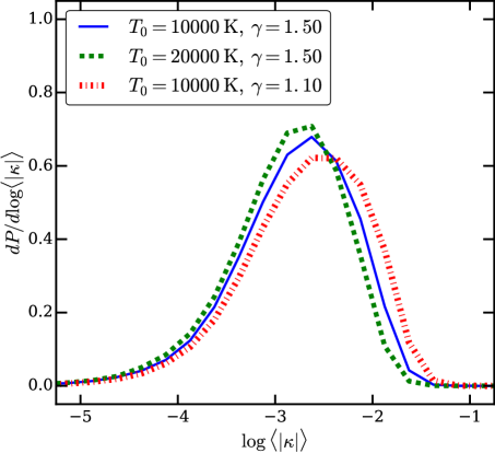
where and are the first and second derivatives of the flux field (with respect to velocity), respectively. Similar to wavelet amplitudes, the curvature can also be affected by the finite S/N of the spectra. To circumvent this difficulty, Becker et al. (2011) fitted a spline curve to the transmitted Ly flux field and used that to compute the curvature. We, however, use a simpler approach of smoothing the flux field by a Gaussian filter of FWHM km s-1 (for a similar approach, see Padmanabhan et al., 2015). Fig. 4 (panel C) shows the comparison of the curvature field for the hot and cold models. Similar to the wavelet field, the curvature amplitude is higher for the cold model as compared to the hot model. In this work, we use the curvature PDF to measure and . Fig. 7 shows the sensitivity of the curvature PDF to and . The curvature PDF is shifted to lower values of for hot models as compared to cold models. The curvature PDF is also sensitive to variations in . However, note that the curvature PDF shows less sensitivity to and than the wavelet PDF.
4.1.4 The -parameter probability distribution function (BPDF)
Variations in the thermal parameters change the broadening of the Ly absorption features. One can quantify this by fitting a multi-component Voigt profile to Ly absorption spectra. The lower envelope of the distribution has been used to measure the thermal parameters (Schaye et al., 1999; Bolton et al., 2014; Gaikwad et al., 2017b; Rorai et al., 2018; Hiss et al., 2018, 2019; Telikova et al., 2019). Fitting Voigt profiles to Ly forest spectra is challenging and somewhat subjective. Furthermore the complexity of Ly absorption increases with increasing redshift as the opacity of the IGM increases. We further need to fit a large number of simulated spectra when measuring model in each redshift bin. To facilitate this, we use our VoIgt profile Parameter Estimation Routine (viper) that automatically fits Ly forest spectra with multi-component Voigt profiles (see Gaikwad et al., 2017b, for details). The output of viper consists of best fit values (along with 1 uncertainty) of line center (), H i column density ( ), parameter and significance level of detection for each component. We used viper to fit (see Table 1) mock Ly forest spectra in each redshift bin. The total time taken by viper to fit all the spectra in all redshift bins is million cpu hours. Panels D and E in Fig. 4 show examples of the viper fits (along with residuals) to the cold and hot model, respectively.
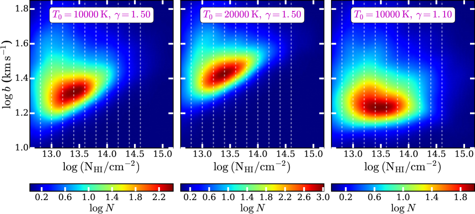
Neither the gas temperature nor the over-density are directly observable quantities. However, the b-parameter of an absorption line is related to the gas temperature while the measured column density( ) is related to the overdensity. The distribution can thus nevertheless be used to measure the thermal parameters. The lower envelope in the distribution is shown to be sensitive to thermal parameters (Webb & Carswell, 1991; Schaye et al., 2000; Bolton et al., 2014; Gaikwad et al., 2017b; Rorai et al., 2018). However, the lower envelope method utilizes fewer points that define the lower cutoff in values at given (but see Hiss et al., 2019; Telikova et al., 2019). Recently, Hiss et al. (2019) have proposed to use the full - 2D distribution to simultaneously measure and . However, this requires to sample the plane densely enough to reduce any statistical fluctuations introduced by binning. This becomes important when there are few observed sightlines in a redshift bin.
To circumvent this difficulty, we have used a modified approach to fit the 2D distribution as shown in Fig. 8 and 9. We divide the plane in different bins centered on with bin width d . We then calculate the 1D distribution of parameters in each bin using KDE.
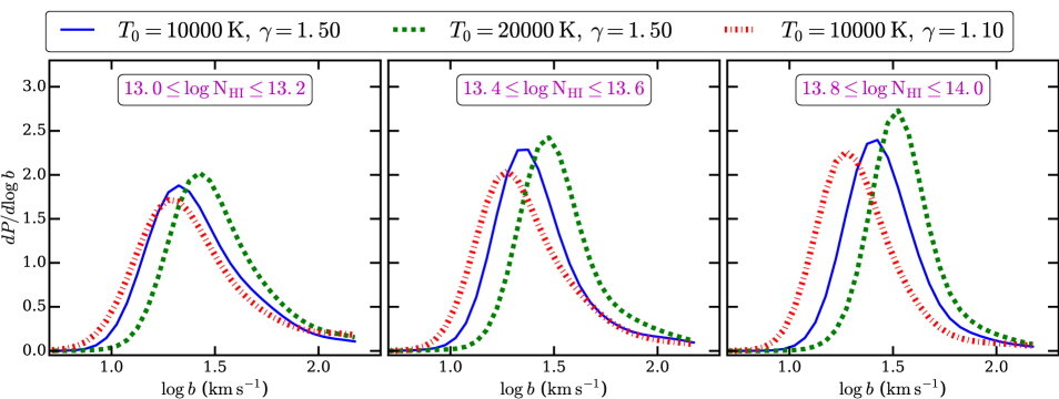
Fig. 9 shows the sensitivity of the distribution to and in the three bins , and . The distribution shows a systematic shift towards higher values for higher models. The distribution is less sensitive to in the range , but it is more sensitive in the range . Thus, the distribution at small column density is rather sensitive to but less sensitive to . This systematic variation in the distribution can change with redshift as the Ly forest is sensitive to different overdensities at different redshifts. We simultaneously use the distribution in all the bins to constrain the thermal parameters. Our method is similar to comparing the full 2D distribution from simulations with observations in the sense that we still use all the data points in the distribution. The only difference is that the size of the bin is larger than that used in the conventional 2D distribution. This effectively reduces the statistical fluctuations due to binning.
4.2 Error estimation of Ly statistics
The best fit values and the associated uncertainties on crucially depend on how accurately we can compute between data and model for a given . The accuracy of the estimation, in turn, depends on (i) the estimated errors (covariance matrix) of the flux statistic and (ii) how finely we sample the plane. Since we use the same method/code to derive the flux statistics from observations and simulations, numerical or computational systematics affecting the flux statistics should cancel out in the (and hence ) estimation.
We have considered two possible ways to calculate the error on each flux statistics: (i) using bootstrap errors estimated from observed data and (ii) deriving the flux statistics and computing the error from 100 simulated mock samples (Rollinde et al., 2013). The second method is not suitable in our case as these errors depend on and . This is especially true for the flux statistics WS, CS and BPDF because variation of thermal parameters shifts the PDF to the right or left i.e., along axis. We also estimate the covariance matrix using the bootstrap method. The bootstrap errors are found to be slowly converging as the diagonal elements of the covariance matrix converge faster than the off-diagonal ones. We find that the diagonal elements computed from the bootstrap method are smaller by percent than those estimated from the mock samples. This is expected as the bootstrap method usually tends to underestimate the errors (Press et al., 1992). To obtain the covariance matrix, we first inflate the boostrap error by percent. We then calculate the correlation matrix from simulated mocks and rescale it using inflated bootstrap errors. We use this covariance matrix when calculating .
Equally important for the measurements and associated uncertainties is the number of grid points for which is calculated (i.e., how finely we sample the parameter space). In this work, is varied from K to K in steps of K while is varied from to in steps of (at ). The Ly statistics are thus derived for different models. However, we find that the sampling needs to be finer ( K and ) if we want the contours for and to be converged. This is because the uncertainty from joint constraints can be smaller than that from individual statistics. Due to limited computational resources, we populate the field by interpolating all the model statistics on to a finer grid with K and . We find that such a linear interpolation of statistics between different model is accurate to percent. Our approach is similar to that in Walther et al. (2019), except that we use simple linear interpolation instead of an emulator. Emulators are useful when the initial and grid is sparse. In our case, the initial grid is more densely sampled than previous works, hence the linear interpolation of statistics between different model is sufficient.
4.3 Method of constraining thermal parameters
In this work, we measure the thermal parameters by minimizing between the observed PDF/PS () and model PDF/PS (),
| (4) |
where is the covariance matrix for each statistics is calculated as described in previous section. We compute for our grid and find the best fit model that corresponds to the minimum for each statistics. We then calculate the uncertainty on the parameters by marginalizing over contours ( for 2 parameters + normalization, Avni, 1976). For the wavelet statistics, the observed and model PDFs depend on an additional parameter, the wavelet scale . To perform simultaneous measurements of and using the wavelet statistics, we add the from different wavelet scales km s-1 i.e., . Similarly, the observed and model BPDF depends on bins. In this case, we add from different bins ( , , ). When performing the measurements from combined statistics, we add the from all the statistics under consideration,
| (5) |
In this work, we ignore the correlation among different statistics for simplicity. Hence the statistical uncertainty on in joint constraints may be somewhat underestimated.
4.4 Validation of our approach using mock data
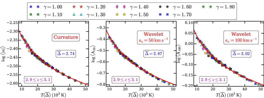
Before measuring the thermal parameters from observations, we demonstrate the accuracy of our method in recovering the thermal parameters with an end-to-end test on mock data created from our fiducial hydro-simulation(s) and from the much larger dynamic range simulation from the Sherwood simulation suite (computed with cosmological parameters similar to what we use in our models). This is with the aim to (i) test the sensitivity of statistics to thermal parameters, (ii) study the degeneracy between thermal parameters, (iii) quantify the accuracy of the method, (iv) check if there are any systematic effects between true and recovered thermal parameters, (v) check if the simulations are sufficiently converged and (vi) test for the effect of Jeans smoothing.
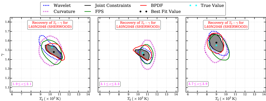
The effect of box size and resolution on statistics of the Ly forest using a range of Sherwood simulations are discussed in online supplementary appendix F. As shown in Fig. 26 to 31, the L10N512 simulation used in this work is sufficiently converged for the corresponding Sherwood model. To test how well our models can recover the thermal parameters, we generate Ly forest statistics in three redshift bins from mock data based on the L40N2048 simulations in the Sherwood suite which has the same resolution and four times larger box size than our fiducial hydro-simulation The flux statistics are generated from skewers as explained in §3. The mock data and our model spectra both closely mimic the properties of the observed sample e.g. number of QSOs, S/N, resolution and redshift path length in the corresponding redshift bin. The errors for each statistics are calculated as discussed in §4.2. When using FPS, BPDF, wavelet and curvature PDF to characterise the thermal parameters we compute the between model and mock data (see §4.2 for details).
Fig. 10 shows the recovery of thermal parameters using our models and the mock data generated from the L40N2048 Sherwood simulation. For all four statistics, the true thermal parameters of the mock data are within the contours and are thus close to the best fit measured thermal parameters. The true thermal parameters are also well within the contours of the measured values if the four statistics are combined (shown by the black contours and the shaded region). As expected the joint analysis contours are narrower than those from individual statistics. The best fit thermal parameters do not show any systematic deviation from the true thermal parameters indicating that any uncertainty in recovery is likely to be statistical in nature.
4.5 The effect of varying Jeans smoothing
The width of absorption features depends on the instantaneous thermal state as well as on the entire past thermal history due to the smoothing effect of the thermal pressure on the spatial distribution of the gas, an effect that has been dubbed Jeans smoothing (Gnedin & Hui, 1998; Peeples et al., 2010; Kulkarni et al., 2015). At the redshifts considered here, well past H i reionization and with the additional heat input from He ii reionization ongoing, the memory of different possible hydrogen reionization histories is expected to be modest. We have verified this by repeating our end-to-end test with mock data from an otherwise identical simulation of the Sherwood suite which has the same instantaneous temperatures, but where hydrogen reionization occurs considerably later (the zr9 Sherwood simulation). The difference in the measured thermal parameters was hardly noticeable ( percent). The range of possible He ii reionization histories consistent with the He ii opacity data is also rather small (Worseck et al., 2019). Hence the effect of the differences in Jeans smoothing for the same instantaneous temperature and different He ii reionization histories is again expected to have a small effect on our measurements of thermal parameters.
4.6 The effect of spatial fluctuation of the temperature-density relation due to inhomogeneous He ii reionization
In reality, He ii reionization will be spatially inhomogeneous and instead of a well defined temperature density relation there will be a range of temperature density relations depending on when the He ii in a particular region was reionized (Rorai et al., 2017b; Upton Sanderbeck & Bird, 2020). In Gaikwad et al. (2020) we have shown that for the equivalent situation during H i reionization assuming a homogeneous UVB model nevertheless recovers the median thermal state reasonably well. We have verified that this should also be the case for He ii reionization by producing flux statistics for mock spectra obtained with a wide range of temperature density relations. As the box size of our simulations is much smaller than the expected size of a region where He ii is reionized simultaneously this should mimic the effect of inhomogeneous He ii reionization reasonably well. The thermal parameters measured from these samples of simulated mock spectra with a range of temperature-density relations are indeed within 1 of the median values. We are not sure if this can be interpreted as a systematic bias, but we note that at and after the peak in temperature the inferred values were about 1 lower than the median while at the difference was hardly noticeable.
5 Results
In this section, we present our measurements of and from the kodiaq DR2 sample. In order to make a fair comparison, we (i) derive the statistics from simulations and observations in the same way, (ii) calculate the error on each statistics from simulations and/or observations, (iii) minimize the between data and model and (iv) find the best fit model and the associated uncertainty on the parameters (see §4.3)
5.1 constraints in the redshift range
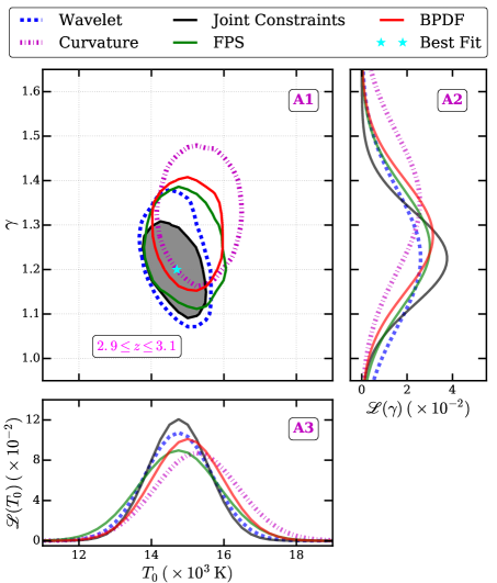
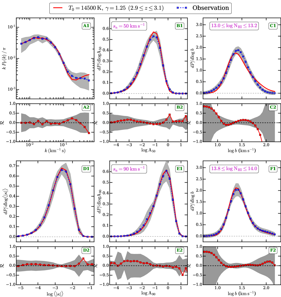
Fig. 11 shows measurements of and in redshift bin . Panel A1 shows the measurements of thermal parameters from individual as well as the combined statistics. The constraints from all four statistics agree with each other within the uncertainties. The constraints on from the curvature statistics are poor compared to those from the other statistics. This is because the curvature PDF is less sensitive to compared to . In previous measurements using curvature statistics, is measured at a characteristic density for an assumed value of . This does not allow for an independent measurement of . It is also evident that and are anti-correlated for the wavelet statistics, BPDF and FPS, while there is little or no correlation between and for the curvature statistics. Panels A2 and A3 show measurements of and marginalizing over and , respectively. The marginalized distributions also show that the and measurements using different statistics are consistent with each other within . Note that the data and model Ly forest spectra are the same in all cases only the method/statistics used to measure is different. In order to get tighter and more robust measurements of and , we also plot the joint constraints for and from all the statistics in panels A1-A3 of Fig. 11. We calculate the joint constraints by adding the between model and data for all the four statistics. For simplicity, we ignore the correlation among different statistics. Hence the statistical uncertainty in joint constraints may be somewhat underestimated. However, as shown in Fig. 10 when combining the statistics, the fiducial is recovered well within . This suggests that the statistical uncertainty for the measurement from the combined statistics is realistic. The joint constrains for and are indeed tighter than the corresponding constraints from any individual statistics. The best fit value ( K and ) for the joint constraints from all the four statistics is shown as the cyan star in panel A1 of Fig. 11 (also see Fig. 43).
Fig. 12 shows the comparison of FPDF, BPDF, wavelet PDF and curvature PDF from observations with the best fit model at . The corresponding residuals are shown in the lower panels. The best fit models for all the statistics are in agreement with the corresponding observations. The per degree of freedom for all the statistics varies in the range (see Fig. 43 and Table 5). The predictions of our best fit model obtained from the joint analysis are thus in reasonably good agreement with observations for all the statistics.
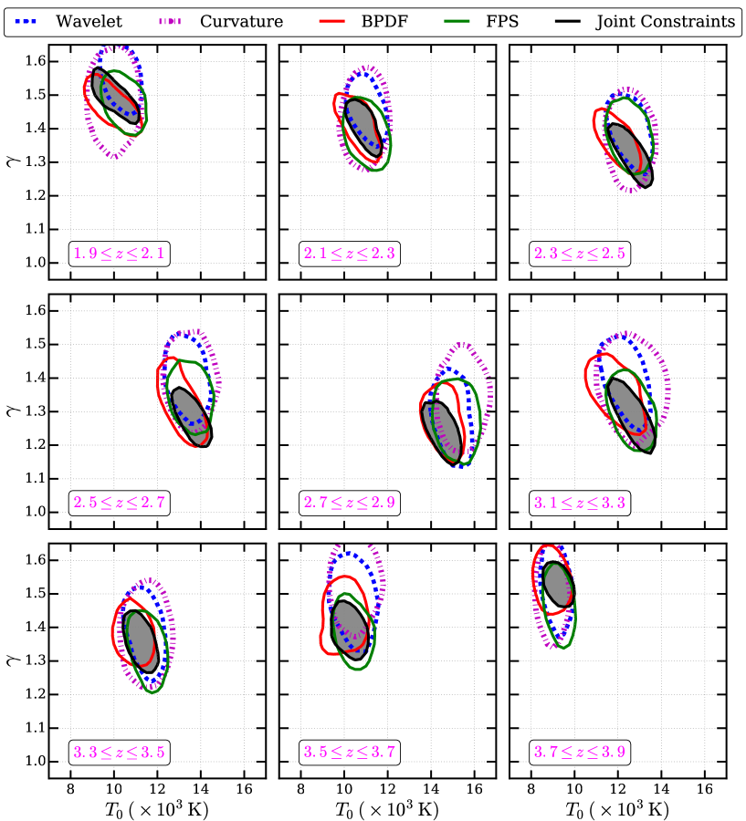
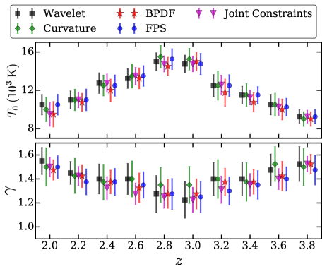
Fig. 13 shows measurements of and in the other redshift bins spanning . In all the redshift bins, the and measurements from the individual statistics are in good agreement with each other. The measurements from the curvature statistics are less tight than those from the other statistics. The uncertainty in using the joint constraints is significantly smaller than that from the individual statistics at all redshifts. The joint constraints are thereby in good agreement with the overlapping regions of all the individual statistics. The variation of the and measurements with redshift is also evident from Fig. 13. As expected the and constraints are anti-correlated in the lower redshift bins where the absorption features probe densities above the mean. With increase in redshift the and correlation becomes weaker, similar to the finding of Walther et al. (2019). This is because at the Ly forest is mostly sensitive to approximately mean cosmic density .
In Fig. 14, we compare the evolution of and from the individual statistics and joint analysis. The () measurements are marginalized over (). We can clearly see an evolution of and with redshift with a clearly identifiable peak in that coincides with a minimum in at . The and measurements from each individual statistics as well as our joint constraints are consistent within in all the redshift bins. As expected, the uncertainty for the joint analysis is smaller than the corresponding uncertainty from the individual flux statistics. The best fit and values show some scatter between neighboring redshift bins for the individual statistics due to the differences in sensitivity of individual statistics to and . The scatter of the best fit values is considerably smaller for the joint measurements.
5.2 Error Budget
| (K) | ||
|---|---|---|
| 2.0 0.1 | 9500 1393 | 1.500 0.096 |
| 2.2 0.1 | 11000 1028 | 1.425 0.133 |
| 2.4 0.1 | 12750 1132 | 1.325 0.122 |
| 2.6 0.1 | 13500 1390 | 1.275 0.122 |
| 2.8 0.1 | 14750 1341 | 1.250 0.109 |
| 3.0 0.1 | 14750 1322 | 1.225 0.120 |
| 3.2 0.1 | 12750 1493 | 1.275 0.129 |
| 3.4 0.1 | 11250 1125 | 1.350 0.108 |
| 3.6 0.1 | 10250 1070 | 1.400 0.101 |
| 3.8 0.1 | 9250 876 | 1.525 0.140 |
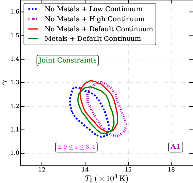
We consider the following important uncertainties when measuring and : (i) modeling uncertainty, (ii) continuum placement uncertainty, (iii) uncertainty due to metal contamination and (iv) cosmological parameter uncertainty. Fig. 15 shows the effect of continuum placement uncertainty and metal contamination uncertainty on our measurements of and from our joint analysis of the four different flux statistics (for . The uncertainty in and due to continuum placement uncertainty (assumed to be percent, see O’Meara et al., 2017) is less than 3 percent. The continuum placement uncertainty mainly affects the mean flux of the observed sample. However, when measuring and , we rescale the optical depth in the simulations to match the observed mean flux. Contamination by narrow metal absorption lines in the observed Ly forest can also potentially bias our and measurements. We thus remove the metal lines from the Ly forest to minimize their effect. However, it is still possible that some metal lines are not identified due to insufficient wavelength coverage in the higher wavelength side of the Ly emission and/or blending effects. By applying a cutoff in the fitted parameters, we show in Fig. 15 that the contribution of such metal lines to the uncertainty is not larger than percent. Similarly, we find that the uncertainty in cosmological parameters can lead to 0.5 percent uncertainty in and . One of the main uncertainties in the and measurements comes from our modeling of the Ly forest. Since we vary the thermal state of the gas by post-processing of gadget-3 simulations, the dynamical impact of pressure smoothing may not have been captured accurately. We find that the effect of pressure smoothing on the and uncertainty is below percent. We refer the reader to online supplementary appendix H for a detailed discussion of the effect of all the above uncertainties on our measurements.
Table 2 provides our and measurements at different redshifts. In Table 6 we give and errors contributed by various above listed uncertainties. The continuum placement uncertainty is systematic, while the other uncertainties are statistical in nature. We add the statistical uncertainties in quadrature while the systematic uncertainty is additive in nature. In the rest of the paper, we show and discuss constraints on and with total uncertainties as given in Table 2.
5.3 Evolution of and
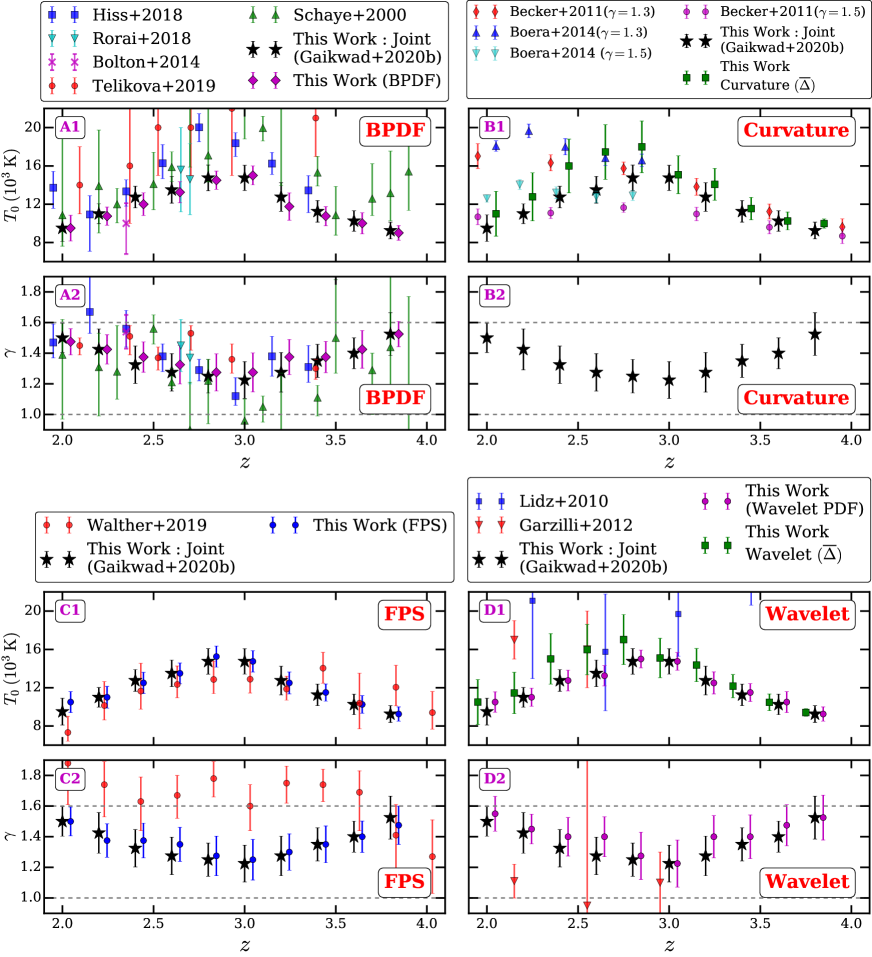
Fig. 16 shows the evolution of and (as given in Table 2 and Table 6) from the joint analysis with total uncertainty in the redshift range . Initially () is small (large) at then it increases (decreases) attaining a maximum (minimum) at . Subsequently () decreases (increases) at . As we will discuss in §6, the peak in the evolution of and is due to the additional heating from He ii reionization. Such a peak in evolution has been suggested based on other published measurements, but note the rather large scatter between different measurements (see Fig. 16 and Fig. 48). Our measurements show for the first time a well defined peak and the expected smooth evolution of and in the redshift range , consistently for all four different flux statistics. We attribute this to the following main differences of our study: (i) our observed sample contains a larger number of QSO sightlines than previous studies, (ii) the simulated Ly forest in our analysis is generated for a finely sampled grid than in previous studies, (iii) we treat the data and simulations on an exact equal footing i.e., our simulated mock spectra are mimicked to match the observed sample, (iv) we apply the same procedure/algorithm to calculate the Ly flux and Voigt profile statistics to observed and simulated spectra (v) by combining the measurements from different statistics, we mitigate possible biases of the individual flux statistics.
5.4 Comparison with other measurements
| Curvature | Wavelet | Wavelet | |
|---|---|---|---|
| km s-1 | km s-1 | ||
| 2.0 | 4.85 | 4.95 | 5.37 |
| 2.2 | 4.57 | 4.30 | 4.98 |
| 2.4 | 3.90 | 3.89 | 4.37 |
| 2.6 | 3.54 | 3.56 | 4.01 |
| 2.8 | 3.19 | 3.26 | 3.50 |
| 3.0 | 2.74 | 2.87 | 3.02 |
| 3.2 | 2.48 | 2.53 | 2.67 |
| 3.4 | 2.17 | 2.16 | 2.27 |
| 3.6 | 2.00 | 1.90 | 2.25 |
| 3.8 | 2.08 | 1.90 | 2.72 |
We now compare the and measurements from this work with that from the literature. Fig. 16 shows a compilation of and measurements from various papers. and have been measured in the past (with variants) of the same four different statistics we have used here. In order to do a fair comparison, we compare our measured and from the joint analysis and the individual statistics with the corresponding statistics from the literature.
5.4.1 Comparison with measurments from
In panel A1 and A2 of Fig. 16, we compare our thermal parameter evolution with that from Schaye (2001); Bolton et al. (2014); Rorai et al. (2018); Hiss et al. (2018, 2019); Telikova et al. (2019) obtained using the distribution. This method is based on fitting the Ly forest spectra with Voigt profiles and defining a lower envelope of the 2D distribution. The motivation behind this is that for the absorption components with low the broadening should be dominated by thermal broadening.
Our and measurements from this statistics are consistent within with that of Bolton et al. (2014); Rorai et al. (2018). The measurements by Hiss et al. (2018); Telikova et al. (2019) are in good agreement with our measurements. However, their measurements are significantly higher than our measurements at . Fitting a lower envelope to the distribution although well motivated, is somewhat subjective. Finding a lower envelope in an objective way is difficult (but see Telikova et al., 2019; Hiss et al., 2019). The lower envelope is found by iteratively rejecting the lines with low parameter until convergence is achieved. More (less) rejection of low parameter lines can lead to systematically higher (lower) inferred temperatures. However, the high values of of Hiss et al. (2018); Telikova et al. (2019) obtained from the distribution are not consistent with the measurements obtained using e.g. the FPS by Walther et al. (2019).
Manual Voigt profile fitting is labour intensive and the number of Voigt components obtained from observations is rather limited in many analyses and often the plane is sampled poorly. To avoid these systematic biases, we use the 1D distribution (BPDF) computed in different bins. The BPDF does not rely on rejecting low parameters to find a lower envelope. At the same time the BPDF statistics is sensitive to both and (see online supplementary appendix 4.1.4 for details). Our method of measuring and using Voigt profile parameters is thus significantly different from that used in the literature. Unlike previous work, our and measurements using the BPDF statistics are consistent with our measurements using the other statistics as shown in Fig. 14.
5.4.2 Comparison with measurments from curvature statistics
In panel B1 and B2 of Fig. 16, we compare our thermal parameter evolution with that from Becker et al. (2011); Boera et al. (2014) obtained using the curvature statistics. These authors measured by measuring the temperature at a characteristic density ( ) that is a one-to-one empirical function of the mean of the absolute curvature irrespective of . To map to the temperature at cosmic mean density , one needs to however assume a value of .
In Fig. 14 we show the measurement of thermal parameters using the PDF of the curvature statistics. To make a more direct comparison between our measurement with that from Becker et al. (2011); Boera et al. (2014), we also calculate the using the characteristic (over-)density method. Fig. 17 and Table 3 shows the probed by the curvature statistics in our simulations. The evolution of from this work is in good agreement with that from Becker et al. (2011). We obtain the one-to-one empirical relation between mean absolute curvature and temperature at (as shown by the red curve in Fig. 17). For a given observed mean absolute curvature, we measure the temperature at . We convert the temperature at into using this empirical relation assuming a range of . For this we use the values (with 1 uncertainty) from our joint constraints. The green squares in panel B1 of Fig. 16 show our measurements using the method. The errors on the measurements for the method account for the uncertainty in only.
In Fig. 16, we also show the measurements using the method and that using the joint analysis. The best fit values from the method are systematically higher than that from the joint analysis as well as those obtained using the curvature PDF (see Fig. 14) at . The method assumes that most of the absorption in the Ly forest at any given redshift is associated with densities . When converting temperature at to , one assumes a single value. However, in a realistic scenario the Ly absorption will arise from a range in densities. Unlike the method, the measured in our joint analysis (using PDFs and PS) is contributed by Ly absorption coming from all densities. We suspect this to be the most likely reason for the systematically larger obtained with the method. Another interesting feature of the evolution obtained using the method is that the uncertainty of the measurements increases with decreasing redshift. This is mainly because of the uncertainty in and the increase of at lower redshifts.
At , our measurements from the method are consistent with that from Becker et al. (2011) irrespective of the assumed value of . This is because the Ly forest at these redshifts is sensitive to densities close to the cosmic mean density . This is reflected in the smaller uncertainty of the measurements at . As decreases () in our joint measurements at , increases and is in good agreement with that from Becker et al. (2011); Boera et al. (2014) for . At , increases from 1.2 to 1.5, and our measurement using the method is consistent with that from Becker et al. (2011); Boera et al. (2014) for .
5.4.3 Comparison with measurements from the FPS
Panel C1 and C2 compares our measurements (FPS and joint analysis) with those from Walther et al. (2019) using the FPS statistics. Similar to this work, Walther et al. (2019) measured the and evolution using the FPS calculated from the kodiaq DR2 sample. However, their sample selection criteria is different from ours. Despite this the FPS from our work is in good agreement with that from Walther et al. (2019). Fig. 16 shows that our measurements are also in good agreement (within uncertainty) with their measurements. Note, however, that our measurements are systematically larger (albeit within the errors) than their measurements at . The difference in the evolution is more pronounced. Our evolution shows a minimum at while their measurement shows a nearly flat at .
Since the observed FPS are in good agreement with each other, the moderate differences in the measurements are likely to come from differences in the simulations/analysis. Walther et al. (2019) vary , and the pressure smoothing scale as a free parameter using the OH17 UVB. They derive a single pressure smoothing scale at a given redshift for the entire simulation box using a cutoff in the 3D real space flux power spectrum that is calculated without accounting for peculiar velocity and thermal broadening. In reality, the pressure smoothing scale is not an independent parameter. This is because the pressure smoothing scale is set by temperature and density of the gas particles i.e., . Simultaneous fitting of and can result in degeneracies of (see Fig. 6, Fig. 6 in Rorai et al., 2018; Walther et al., 2019, respectively). An overestimation of can result in a systematic decrease and increase in and , respectively. In our simulations, the pressure smoothing scale is set by the density and temperature of each SPH particle which varies for each particle. Hence effectively we fit as two free parameters to match the simulations with observations. It is also important to note that all UVB models predict at (for equilibrium as well as non-equilibrium evolution of the ionization). As we show in §6 the evolution in Walther et al. (2019) is very difficult to reproduce with any UVB model.
5.4.4 Comparison of measurements from the wavelet statistics
We compare our and measurements using the wavelet statistics with those from Lidz et al. (2010) and Garzilli et al. (2012) in panel D1 and D2 of Fig. 16 respectively. Our measurements from the wavelet analysis are more consistent with other flux statistics than those of Lidz et al. (2010) and Garzilli et al. (2012). The main difference between previous works and this work are the observations and the methodology we use. Our observed sample size () is larger than that of previous studies using wavelet statistics (40 and 20 for Lidz et al. (2010) and Garzilli et al. (2012) respectively). To mitigate noise effects, Lidz et al. (2010) apply boxcar smoothing on the wavelet field which somewhat reduces the sensitivity of the wavelets to and . In this work, we compute the PDF from the unsmoothed wavelet field using kernel density estimation which converges faster than using a simple histogram reducing the effect of noise on the PDF. In addition we simultaneously measure and at wavelet scales km s-1. Lidz et al. (2010) and Garzilli et al. (2012) use only one wavelet scale at a time to measure and . As a result, our and constraints are tighter than that of Lidz et al. (2010) and Garzilli et al. (2012).
We find the characteristic over-density ( ) probed by the wavelet statistics for km s-1 and km s-1, respectively (see Fig. 17). Table 3 also summarizes the redshift evolution of for these two wavelet scales. The characteristic density varies similarly with other wavelet scales. We find that the scatter in the empirical relation increases with increasing wavelet scales reducing the sensitivity to . This is expected as on large scales the baryons trace the dark matter density field and large scales are less sensitive to variations in . We also measure using the method for the wavelet statistics assuming the evolution from our joint analysis. The values for all the wavelet scales are very similar. In Fig. 16, we show the values obtained using the method (green squares, for km s-1) and that obtained using the joint analysis (black stars). The values from the two methods are in good agreement with each other (within ).
6 Discussion: Implication for UVB models and HeII reionization
In this section, we compare our measurements of and with predictions from published spatially homogeneous UVB models for the effect of He ii reionization on the thermal evolution of the IGM. In Fig. 18, we compare the observed evolution with that predicted by the UVB models of \al@haardt2012,onorbe2017,khaire2019a,puchwein2019; \al@haardt2012,onorbe2017,khaire2019a,puchwein2019; \al@haardt2012,onorbe2017,khaire2019a,puchwein2019; \al@haardt2012,onorbe2017,khaire2019a,puchwein2019 and FG20. We use cite to obtain the evolution of and for these UVB models, post-processing gadget-3 outputs.
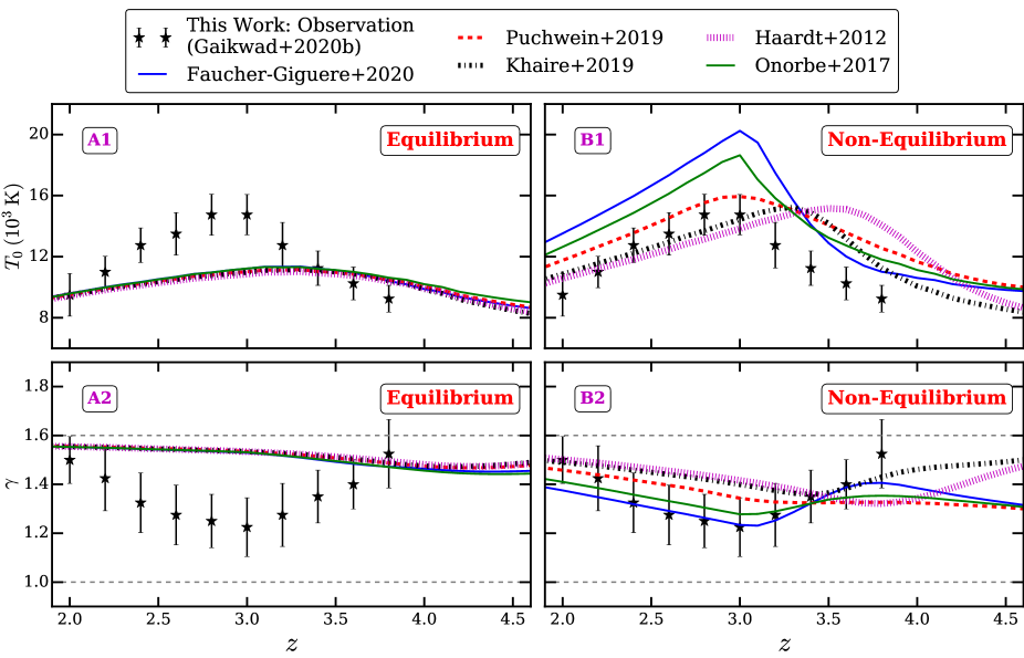
6.1 Equilibrium vs Non-equilibrium UVB models
Panels A1 and A2 in Fig. 18 show that the different UVB models with equilibrium ionization evolution show a very similar evolution in the redshift range irrespective of the temperature after H i reionization. The observed () is systematically larger (smaller) than that predicted from equilibrium models at ( ). It appears that it is not possible to reproduce the higher (smaller ) seen in the observed data with UVB models assuming equilibrium ionization evolution. With equilibrium ionization evolution, one assumes that the gas is ionized instantaneously as the ionizing radiation field is turned on. Because of this, the He ii fraction in equilibrium model is systematically underestimated (Puchwein et al., 2015; Gaikwad et al., 2019). Since the photo-heating is proportional to the He ii fraction, the temperature is underestimated. Similarly, the He ii fraction depends on density in photo-ionization equilibrium and as a result the photo-heating of the gas is density dependent. As shown in Gaikwad et al. (2019) the density dependent photo-heating rates result in in equilibrium ionization models.
The He ii reionization will in reality also be spatially inhomogeneous, and spatially homogeneous UVB models can only give an average evolution of the thermal history. However, in any given place the He iii ionization fronts will move too fast for equilibrium ionization evolution to be a good approximation. We have thus also implemented physically well motivated non-equilibrium ionization evolution in cite. Panels B1 and B2 in Fig. 18 show the comparison of our and measurements with the prediction from UVB models assuming non-equilibrium evolution. The () values are systematically larger (smaller) than in the corresponding equilibrium models and the differences between the different UVB models are larger. The non-equilibrium predictions by all the UVB models also show a more pronounced temperature peak. This peak is generally somewhat higher than that in our measurements from the observations and occurs in some of the models also somewhat earlier.
6.2 The temperature peak/rise due to HeII reionization predicted by spatially homogeneous UVB models
| UVB Model | [a] | [b] | [c] | [d] |
|---|---|---|---|---|
| FG20 | 3.2 | 0.3 | 0.70 0.10 | 2.97 |
| P19 | 3.5 | 0.8 | 0.90 0.20 | 3.05 |
| KS19 | 3.6 | 0.8 | 1.00 0.20 | 2.43 |
| HM12 | 4.0 | 1.0 | 1.00 0.20 | 3.14 |
| OH17 | 3.2 | 0.4 | 0.75 0.15 | 3.09 |
-
a
The redshift of reionization is defined as corresponding to epoch when
-
b
The extent of reionization is defined as . where corresponds to the redshift when respectively.
- c
-
d
Cumulative energy deposited (in ) into the IGM at for non-equilibrium UVB models without scaling the photo-heating rates (see online supplementary appendix J).
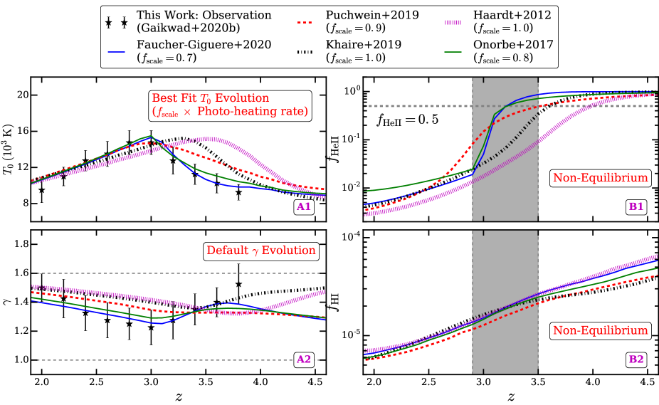
The basic concept of the different UVB models is similar, but there are considerable differences in the detailed assumptions. \al@onorbe2017,faucher2020; \al@onorbe2017,faucher2020 compute photo-ionization and photo-heating rates during ( H i and He ii) reionization differently than \al@haardt2012,khaire2019a,puchwein2019; \al@haardt2012,khaire2019a,puchwein2019; \al@haardt2012,khaire2019a,puchwein2019. To calculate photo-ionization and photo-heating rates during He ii reionization, \al@onorbe2017,faucher2020; \al@onorbe2017,faucher2020 assume the He ii reionization history ( evolution) to be a free parametric function. The reionization history is calibrated to match the observed evolution (Worseck et al., 2019). To compute the photo-heating rates during reionization, \al@onorbe2017,faucher2020; \al@onorbe2017,faucher2020 then use another free parameter namely the total heat injected during He ii reionization (). \al@haardt2012,khaire2019a,puchwein2019; \al@haardt2012,khaire2019a,puchwein2019; \al@haardt2012,khaire2019a,puchwein2019 on the other hand try to predict photo-ionisation and photo-heating rates based on observed source luminosity functions and SEDs and a model of the He ii opacity based on observations. There is thus considerable variety in the assumptions of spatially homogeneous UVB models. As a result the exact time and height of the temperature peak predicted by these models should be considered somewhat uncertain. As can be seen in panel B1/B2 in Fig. 18, the timing of the temperature peak in the \al@onorbe2017,faucher2020; \al@onorbe2017,faucher2020 UVB models agrees very well with the timing of the peak in our measurements. The evolution of in these models is also in better agreement with our measurements than those from \al@haardt2012,khaire2019a,puchwein2019; \al@haardt2012,khaire2019a,puchwein2019; \al@haardt2012,khaire2019a,puchwein2019. However, is systematically larger than our measured values at all redshifts. Given the uncertainty in the amplitude of the photo-heating rates in all the UVB models, we have rescaled the H i, He i and He ii photo-heating rates in order to better match our measured evolution of the thermal parameters. Such a rescaling changes systematically, while the evolution remains largely unaffected.
Panels A1 and A2 in Fig. 19 show the evolution of and for scaled photo-heating rates in the different UVB models. In Table 4, we summarize the photo-heating rate scale factor required in different UVB models to match the observed evolution at (see also Fig. 45 and Fig. 46 for details). As expected, all the rescaled UVB models show a better agreement with the evolution at . However, the evolution at in the rescaled \al@onorbe2017,faucher2020; \al@onorbe2017,faucher2020 UVB models is in much better agreement with our measured values than the \al@haardt2012,khaire2019a,puchwein2019; \al@haardt2012,khaire2019a,puchwein2019; \al@haardt2012,khaire2019a,puchwein2019 UVB models. The shape of the evolution is closely related to the He ii reionization history ( evolution Gaikwad et al., 2019). It is noteworthy here that the reionization history used in the \al@onorbe2017,faucher2020; \al@onorbe2017,faucher2020 UVB models is calibrated to match the observed evolution from Worseck et al. (2019). The good match between the shape of the observed evolution and that predicted by the UVB models with scaled photo-heating rates at suggests that the evolution from our work is in good agreement with the observed evolution from Worseck et al. (2019). Such consistency is important because the evolution of and at is mainly driven by the evolution (see Fig. 5 in Gaikwad et al., 2019). We should here emphasize that the observed dataset, methodology and parameters that we used here are completely complementary to those used to measure the evolution in Worseck et al. (2019).
Despite the good match between observations and the predictions by non-equilibrium \al@onorbe2017,faucher2020; \al@onorbe2017,faucher2020 UVB models, we would like to caution the reader that these UVB models do not account for inhomogeneous He ii reionization and the spatial fluctuations in the He ii ionizing background which are expected to be present. To capture the effects of such spatial fluctuations, will, however require rather challenging high dynamic range radiative transfer simulations (ideally coupled to the hydrodynamics). We hope to do this in future work but caution that it will be very expensive to calibrate such simulations to match the observed data (see Gaikwad et al., 2020).
6.3 Late vs Early HeII reionization
In Fig. 19, we compare the evolution of the He ii and H i fraction predicted by the different UVB models with non-equilibrium ionisation evolution. As already discussed the amount of heat injected into the IGM is coupled to the evolution and we have scaled the photo-heating rates to match the observed evolution. To quantify the differences between the various UVB models, we define the mid point of He ii reionization as the redshift, where . We also define the extent of reionization () as corresponding to the difference between the redshifts when and . These definitions facilitate the comparison of the UVB models quantitatively, but note that they may differ from definitions used in the literature (see Table 4).
The midpoint of He ii reionization in the \al@onorbe2017,faucher2020; \al@onorbe2017,faucher2020 models () is at lower redshift than that for the models by \al@haardt2012,khaire2019a,puchwein2019; \al@haardt2012,khaire2019a,puchwein2019; \al@haardt2012,khaire2019a,puchwein2019. The observed evolution from our measurements is consistent with the relatively late He ii reionization in the \al@onorbe2017,faucher2020; \al@onorbe2017,faucher2020 models. Fig. 19 also shows that the evolution of in the \al@haardt2012,khaire2019a,puchwein2019; \al@haardt2012,khaire2019a,puchwein2019; \al@haardt2012,khaire2019a,puchwein2019 models is more gradual than that in the \al@onorbe2017,faucher2020; \al@onorbe2017,faucher2020 UVB models. The extent of He ii reionization in the \al@onorbe2017,faucher2020; \al@onorbe2017,faucher2020 UVB models is smaller than that in the \al@haardt2012,khaire2019a,puchwein2019; \al@haardt2012,khaire2019a,puchwein2019; \al@haardt2012,khaire2019a,puchwein2019 UVB models (see Table 4). We should note here that the actual duration and heating due to He ii reionization may be different if the spatially inhomogeneous nature of He ii reionization and the resulting fluctuations in the He ii ionizing background are taken into account. With this caveat in mind we note that for the spatially uniform UVB models considered in this work, our measured evolution is consistent with late and rapid He ii reionization.
We refer readers to online supplementary appendix I and J for more details on the effect of the UVB on the evolution of thermal parameters and cumulative energy deposited in to the IGM. In particular, we show the effect of observational and modeling uncertainty in the UVB model on thermal parameters in online supplementary appendices I.1 and I.2. We discuss the likely modification needed for the physically motivated non-equilibrium UVB models to reproduce our measured thermal parameter evolution in online supplementary appendices I.3 and I.4. We discuss the evolution of the cumulative energy deposited in IGM by various UVB models in online supplementary appendix J.
Finally, we emphasize again that even though we use equilibrium KS19 UVB models to vary the thermal parameters in the simulations, our final measured thermal parameter evolution is consistent with the predictions by the physically motivated non-equilibrium evolution for the \al@faucher2020,onorbe2017; \al@faucher2020,onorbe2017 UVB models with moderately reduced photo-heating rates. This gives us additional confidence that our measurements of thermal parameters are robust with regard to observational and modeling systematics.
7 Summary
We have measured the thermal parameters and of the IGM at using 103 high-resolution, high signal-to-noise QSO absorption spectra drawn from the kodiaq DR2 sample using four different Ly flux statistics. The measurements are calibrated with a suite of simulations based on a high-resolution smoothed particle hydrodynamics simulation post-processed with our IGM thermal history code “Code for Ionization and Temperature Evolution” (cite) that finely samples the grid in and . The salient points of our work are:
-
•
We use a sample of 103 QSO spectra satisfying the following criteria; (i) spectral S/N , (ii) no large spectral gaps and (iii) no identified DLAs or sub-DLAs to avoid systematic biases. We have divided our sample in redshift bins having with centers at . The typical number of lines of sight used per redshift bin is larger than what has been used in previous studies. We have identified metal lines contaminating the Ly forest and replaced them with continuum and added noise. Our simulations, based on L10N512 gadget-3 SPH simulation, sample from K to K in bins of K and from to in bins in of creating a densely sampled grids with thermal parameter variations. The mock spectra created from these simulations account for the redshift path length, finite S/N and instrumental broadening of the spectrograph of the observed sample.
-
•
Using our code “VoIgt profile Parameter Estimation Routine” (viper), we fit the observed and simulated Ly forest spectra with multi-component Voigt profiles. We derive 6 flux statistics for observed and simulated spectra: (i) flux power spectrum (FPS), (ii) wavelet statistics (iii) curvature statistics, (iv) distribution function (BPDF), (v) transmitted flux probability distribution function (FPDF) and (iv) H i column density distribution function (CDDF). The observed FPS, FPDF, CDDF and mean flux evolution from our sample is in good agreement with measurements in the literature. By varying one parameter at a time, we show the sensitivity of these statistics to thermal parameters of the IGM.
-
•
We measure the thermal parameters and in the redshift range by quantitatively comparing four of the six flux statistic, namely FPS, wavelet, curvature and BPDF statistics. The and measurements using different statistics are consistent with each other within at all redshifts. By combining the four statistics we thus find joint constraints on and that are more robust and tightly constrained than the measured values from the individual statistics. We estimate the total uncertainty on and by accounting for the uncertainty due to continuum fitting, metal line contamination, cosmological parameters and modeling uncertainties. In this work, we ignore the correlation among different statistics for simplicity. Hence the statistical uncertainty of in joint constraints may be somewhat underestimated. However, our recovery using the Sherwood simulation suite suggests that the uncertainty is not seviorly underestimated. We find that our measured varies from K at to K at to K at , while evolves from at to at to at . We robustly detect a maximum in and minimum in that occur simultaneously at .
-
•
We compare our measurements to the evolution of and predicted by spatially homogeneous UVB background models of \al@haardt2012,onorbe2017,khaire2019a,puchwein2019,faucher2020; \al@haardt2012,onorbe2017,khaire2019a,puchwein2019,faucher2020; \al@haardt2012,onorbe2017,khaire2019a,puchwein2019,faucher2020; \al@haardt2012,onorbe2017,khaire2019a,puchwein2019,faucher2020; \al@haardt2012,onorbe2017,khaire2019a,puchwein2019,faucher2020 assuming equilibrium and non-equilibrium ionization evolution. Our temperature measurements are difficult to reproduce assuming equilibrium ionization evolution. Our measurements are, however, in good agreement with the thermal evolution predicted by the UVB models that have been calibrated to match the observed He ii opacity evolution (\al@onorbe2017,faucher2020; \al@onorbe2017,faucher2020) if we assume non-equilibrium ionization evolution and reduce the photo-heating rates in these models by a moderate factor 0.7-0.8. The timing of the peak in our measured temperatures due to the extra heat input during He ii reionization appears thus to be nicely consistent with the timing of He ii reionization inferred from the He ii opacity evolution and appears to be rather rapid. Our measured temperatures are also (to varying degree) systematically lower than those in the other three models. These three models predict He ii reionization to be more extended and either an onset of the temperature rise (P19) or a timing of the peak that is too early (\al@haardt2012,khaire2019a; \al@haardt2012,khaire2019a) to be consistent with our temperature measurements.
The simulations used to calibrate our temperature measurements assume time varying but spatially uniform UVB models. While spatial fluctuations in the He ii ionizing background are clearly important during He ii reionization (), simulating these self-consistently is beyond the scope of the current work. Large suites of high dynamic range, large scale, multi-frequency cosmological radiative transfer simulations will be required to capture this effect accurately and to sample the observational uncertainties regarding relevant properties of the ionizing sources. We hope to perform such simulations in future. The tests we have performed and our experience with hydrogen reionization suggest that modeling the thermal evolution with homogeneous UVB models should nevertheless recover the evolution of the (median) thermal state of the IGM not only after but also before overlap of He iii regions reasonably well.
Acknowledgments
We thank the DiRAC@Durham facility managed by the Institute for Computational Cosmology on behalf of the STFC DiRAC HPC Facility (www.dirac.ac.uk). The equipment was funded by BEIS capital funding via STFC capital grants ST/P002293/1, ST/R002371/1 and ST/S002502/1, Durham University and STFC operations grant ST/R000832/1. DiRAC is part of the National e-Infrastructure. Computations in this work were also performed using the Perseus cluster at IUCAA, the HPC cluster at NCRA and the CALX machines at IoA. Support by ERC Advanced Grant 320596 ‘The Emergence of Structure During the Epoch of reionization’ is gratefully acknowledged. PG and MGH acknowledge the support of the UK Science and Technology Facilities Council (STFC). TRC acknowledges support of the Department of Atomic Energy, Government of India, under project no. 12-R&D-TFR-5.02-0700. We thank J. Bolton for making the Sherwood simulation suite available to our work. The Sherwood simulations were performed using the Curie supercomputer at the Tre Grand Centre de Calcul (TGCC), and the DiRAC Data Analytic system at the University of Cambridge, operated by the University of Cambridge High Performance Computing Service on behalf of the STFC DiRAC HPC Facility (www.dirac.ac.uk). This equipment was funded by BIS National E-infrastructure capital grant (ST/K001590/1), STFC capital grants ST/H008861/1 and ST/H00887X/1, and STFC DiRAC Operations grant ST/K00333X/1. DiRAC is part of the National E- Infrastructure. We thank Vid Irsic, Ewald Puchwein and Jamie Bolton for useful comments on the manuscript.
Data Availability
The data underlying this article are available in the article and in its online supplementary material.
References
- Almgren et al. (2013) Almgren A. S., Bell J. B., Lijewski M. J., Lukić Z., Van Andel E., 2013, ApJ, 765, 39
- Avni (1976) Avni Y., 1976, ApJ, 210, 642
- Becker & Bolton (2013) Becker G. D., Bolton J. S., 2013, MNRAS, 436, 1023
- Becker et al. (2011) Becker G. D., Bolton J. S., Haehnelt M. G., Sargent W. L. W., 2011, MNRAS, 410, 1096
- Becker et al. (2013) Becker G. D., Hewett P. C., Worseck G., Prochaska J. X., 2013, MNRAS, 430, 2067
- Boera et al. (2014) Boera E., Murphy M. T., Becker G. D., Bolton J. S., 2014, MNRAS, 441, 1916
- Boera et al. (2019) Boera E., Becker G. D., Bolton J. S., Nasir F., 2019, ApJ, 872, 101
- Bolton & Haehnelt (2007) Bolton J. S., Haehnelt M. G., 2007, MNRAS, 382, 325
- Bolton et al. (2005) Bolton J. S., Haehnelt M. G., Viel M., Springel V., 2005, MNRAS, 357, 1178
- Bolton et al. (2012) Bolton J. S., Becker G. D., Raskutti S., Wyithe J. S. B., Haehnelt M. G., Sargent W. L. W., 2012, MNRAS, 419, 2880
- Bolton et al. (2014) Bolton J. S., Becker G. D., Haehnelt M. G., Viel M., 2014, MNRAS, 438, 2499
- Bolton et al. (2017) Bolton J. S., Puchwein E., Sijacki D., Haehnelt M. G., Kim T.-S., Meiksin A., Regan J. A., Viel M., 2017, MNRAS, 464, 897
- Calura et al. (2012) Calura F., Tescari E., D’Odorico V., Viel M., Cristiani S., Kim T. S., Bolton J. S., 2012, MNRAS, 422, 3019
- Calverley et al. (2011) Calverley A. P., Becker G. D., Haehnelt M. G., Bolton J. S., 2011, MNRAS, 412, 2543
- Carswell et al. (1982) Carswell R. F., Whelan J. A. J., Smith M. G., Boksenberg A., Tytler D., 1982, MNRAS, 198, 91
- Chang et al. (2012) Chang P., Broderick A. E., Pfrommer C., 2012, ApJ, 752, 23
- Choudhury et al. (2001) Choudhury T. R., Srianand R., Padmanabhan T., 2001, ApJ, 559, 29
- Cirelli et al. (2009) Cirelli M., Iocco F., Panci P., 2009, J. Cosmology Astropart. Phys., 2009, 009
- Croft et al. (2002) Croft R. A. C., Weinberg D. H., Bolte M., Burles S., Hernquist L., Katz N., Kirkman D., Tytler D., 2002, ApJ, 581, 20
- D’Aloisio et al. (2020) D’Aloisio A., McQuinn M., Trac H., Cain C., Mesinger A., 2020, arXiv e-prints, p. arXiv:2002.02467
- Day et al. (2019) Day A., Tytler D., Kambalur B., 2019, MNRAS, 489, 2536
- Faucher-Giguère (2020) Faucher-Giguère C.-A., 2020, MNRAS, 493, 1614
- Faucher-Giguère et al. (2008) Faucher-Giguère C.-A., Lidz A., Hernquist L., 2008, Science, 319, 52
- Faucher-Giguère et al. (2009) Faucher-Giguère C.-A., Lidz A., Zaldarriaga M., Hernquist L., 2009, ApJ, 703, 1416
- Gaikwad et al. (2017a) Gaikwad P., Khaire V., Choudhury T. R., Srianand R., 2017a, MNRAS, 466, 838
- Gaikwad et al. (2017b) Gaikwad P., Srianand R., Choudhury T. R., Khaire V., 2017b, MNRAS, 467, 3172
- Gaikwad et al. (2018) Gaikwad P., Choudhury T. R., Srianand R., Khaire V., 2018, MNRAS, 474, 2233
- Gaikwad et al. (2019) Gaikwad P., Srianand R., Khaire V., Choudhury T. R., 2019, MNRAS, 490, 1588
- Gaikwad et al. (2020) Gaikwad P., et al., 2020, arXiv e-prints, p. arXiv:2001.10018
- Garzilli et al. (2012) Garzilli A., Bolton J. S., Kim T. S., Leach S., Viel M., 2012, MNRAS, 424, 1723
- Garzilli et al. (2017) Garzilli A., Boyarsky A., Ruchayskiy O., 2017, Physics Letters B, 773, 258
- Gnedin & Hui (1998) Gnedin N. Y., Hui L., 1998, MNRAS, 296, 44
- Haardt & Madau (1996) Haardt F., Madau P., 1996, ApJ, 461, 20
- Haardt & Madau (2012) Haardt F., Madau P., 2012, ApJ, 746, 125
- Hiss et al. (2018) Hiss H., Walther M., Hennawi J. F., Oñorbe J., O’Meara J. M., Rorai A., Lukić Z., 2018, ApJ, 865, 42
- Hiss et al. (2019) Hiss H., Walther M., Oñorbe J., Hennawi J. F., 2019, ApJ, 876, 71
- Hui & Gnedin (1997) Hui L., Gnedin N. Y., 1997, MNRAS, 292, 27
- Iršič et al. (2017a) Iršič V., et al., 2017a, Phys. Rev. D, 96, 023522
- Iršič et al. (2017b) Iršič V., Viel M., Haehnelt M. G., Bolton J. S., Becker G. D., 2017b, Phys. Rev. Lett., 119, 031302
- Khaire (2017) Khaire V., 2017, MNRAS, 471, 255
- Khaire & Srianand (2015) Khaire V., Srianand R., 2015, ApJ, 805, 33
- Khaire & Srianand (2019) Khaire V., Srianand R., 2019, MNRAS, 484, 4174
- Khaire et al. (2016) Khaire V., Srianand R., Choudhury T. R., Gaikwad P., 2016, MNRAS, 457, 4051
- Khaire et al. (2019) Khaire V., et al., 2019, MNRAS, 486, 769
- Kim et al. (2004) Kim T. S., Viel M., Haehnelt M. G., Carswell R. F., Cristiani S., 2004, MNRAS, 347, 355
- Kim et al. (2007) Kim T. S., Bolton J. S., Viel M., Haehnelt M. G., Carswell R. F., 2007, MNRAS, 382, 1657
- Kim et al. (2013) Kim T. S., Partl A. M., Carswell R. F., Müller V., 2013, A&A, 552, A77
- Kirkman et al. (2005) Kirkman D., et al., 2005, MNRAS, 360, 1373
- Kulkarni & Fall (1993) Kulkarni V. P., Fall S. M., 1993, ApJ, 413, L63
- Kulkarni et al. (2015) Kulkarni G., Hennawi J. F., Oñorbe J., Rorai A., Springel V., 2015, ApJ, 812, 30
- Kulkarni et al. (2019) Kulkarni G., Worseck G., Hennawi J. F., 2019, MNRAS, 488, 1035
- Lidz et al. (2007) Lidz A., McQuinn M., Zaldarriaga M., Hernquist L., Dutta S., 2007, ApJ, 670, 39
- Lidz et al. (2010) Lidz A., Faucher-Giguère C.-A., Dall’Aglio A., McQuinn M., Fechner C., Zaldarriaga M., Hernquist L., Dutta S., 2010, ApJ, 718, 199
- Liu et al. (2020) Liu H., Qin W., Ridgway G. W., Slatyer T. R., 2020, arXiv e-prints, p. arXiv:2008.01084
- Lukić et al. (2015) Lukić Z., Stark C. W., Nugent P., White M., Meiksin A. A., Almgren A., 2015, MNRAS, 446, 3697
- Lusso et al. (2014) Lusso E., et al., 2014, ApJ, 784, 176
- Maitra et al. (2019) Maitra S., Srianand R., Petitjean P., Rahmani H., Gaikwad P., Choudhury T. R., Pichon C., 2019, MNRAS, p. 2422
- Maitra et al. (2020) Maitra S., Srianand R., Gaikwad P., Choudhury T. R., Paranjape A., Petitjean P., 2020, arXiv e-prints, p. arXiv:2005.05346
- McDonald (2003) McDonald P., 2003, ApJ, 585, 34
- McDonald & Miralda-Escudé (2001) McDonald P., Miralda-Escudé J., 2001, ApJ, 549, L11
- Miralda-Escudé & Rees (1994) Miralda-Escudé J., Rees M. J., 1994, MNRAS, 266, 343
- Murphy et al. (2019) Murphy M. T., Kacprzak G. G., Savorgnan G. A. D., Carswell R. F., 2019, MNRAS, 482, 3458
- Nasir et al. (2016) Nasir F., Bolton J. S., Becker G. D., 2016, MNRAS, 463, 2335
- Nath & Biermann (1993) Nath B. B., Biermann P. L., 1993, MNRAS, 265, 241
- Oñorbe et al. (2017) Oñorbe J., Hennawi J. F., Lukić Z., 2017, ApJ, 837, 106
- Oñorbe et al. (2019) Oñorbe J., Davies F. B., Lukić Z., Hennawi J. F., Sorini D., 2019, MNRAS, 486, 4075
- O’Meara et al. (2015) O’Meara J. M., et al., 2015, AJ, 150, 111
- O’Meara et al. (2017) O’Meara J. M., Lehner N., Howk J. C., Prochaska J. X., Fox A. J., Peeples M. S., Tumlinson J., O’Shea B. W., 2017, AJ, 154, 114
- Padmanabhan et al. (2014) Padmanabhan H., Choudhury T. R., Srianand R., 2014, MNRAS, 443, 3761
- Padmanabhan et al. (2015) Padmanabhan H., Srianand R., Choudhury T. R., 2015, MNRAS, 450, L29
- Park et al. (2016) Park H., Shapiro P. R., Choi J.-h., Yoshida N., Hirano S., Ahn K., 2016, ApJ, 831, 86
- Peeples et al. (2010) Peeples M. S., Weinberg D. H., Davé R., Fardal M. A., Katz N., 2010, MNRAS, 404, 1281
- Planck Collaboration et al. (2014) Planck Collaboration et al., 2014, A&A, 571, A16
- Press et al. (1992) Press W. H., Teukolsky S. A., Vetterling W. T., Flannery B. P., 1992, Numerical recipes in FORTRAN. The art of scientific computing
- Puchwein et al. (2012) Puchwein E., Pfrommer C., Springel V., Broderick A. E., Chang P., 2012, MNRAS, 423, 149
- Puchwein et al. (2015) Puchwein E., Bolton J. S., Haehnelt M. G., Madau P., Becker G. D., Haardt F., 2015, MNRAS, 450, 4081
- Puchwein et al. (2019) Puchwein E., Haardt F., Haehnelt M. G., Madau P., 2019, MNRAS, 485, 47
- Rauch et al. (1997) Rauch M., et al., 1997, ApJ, 489, 7
- Rollinde et al. (2013) Rollinde E., Theuns T., Schaye J., Pâris I., Petitjean P., 2013, MNRAS, 428, 540
- Rorai et al. (2017a) Rorai A., et al., 2017a, Science, 356, 418
- Rorai et al. (2017b) Rorai A., et al., 2017b, MNRAS, 466, 2690
- Rorai et al. (2018) Rorai A., Carswell R. F., Haehnelt M. G., Becker G. D., Bolton J. S., Murphy M. T., 2018, MNRAS, 474, 2871
- Samui et al. (2005) Samui S., Subramanian K., Srianand R., 2005, in 29th International Cosmic Ray Conference (ICRC29), Volume 9. p. 215 (arXiv:astro-ph/0505590)
- Schaye (2001) Schaye J., 2001, ApJ, 559, 507
- Schaye et al. (1999) Schaye J., Theuns T., Leonard A., Efstathiou G., 1999, MNRAS, 310, 57
- Schaye et al. (2000) Schaye J., Theuns T., Rauch M., Efstathiou G., Sargent W. L. W., 2000, MNRAS, 318, 817
- Scoccimarro et al. (2012) Scoccimarro R., Hui L., Manera M., Chan K. C., 2012, Phys. Rev. D, 85, 083002
- Shull & Danforth (2020) Shull M., Danforth C., 2020, arXiv e-prints, p. arXiv:2007.02948
- Springel (2005) Springel V., 2005, MNRAS, 364, 1105
- Srianand & Khare (1996) Srianand R., Khare P., 1996, MNRAS, 280, 767
- Stevans et al. (2014) Stevans M. L., Shull J. M., Danforth C. W., Tilton E. M., 2014, ApJ, 794, 75
- Telikova et al. (2019) Telikova K. N., Shternin P. S., Balashev S. A., 2019, ApJ, 887, 205
- Theuns et al. (2000) Theuns T., Schaye J., Haehnelt M. G., 2000, MNRAS, 315, 600
- Theuns et al. (2002a) Theuns T., Zaroubi S., Kim T.-S., Tzanavaris P., Carswell R. F., 2002a, MNRAS, 332, 367
- Theuns et al. (2002b) Theuns T., Schaye J., Zaroubi S., Kim T.-S., Tzanavaris P., Carswell B., 2002b, ApJ, 567, L103
- Upton Sanderbeck & Bird (2020) Upton Sanderbeck P., Bird S., 2020, arXiv e-prints, p. arXiv:2002.05733
- Upton Sanderbeck et al. (2016) Upton Sanderbeck P. R., D’Aloisio A., McQuinn M. J., 2016, MNRAS, 460, 1885
- Viel et al. (2004a) Viel M., Haehnelt M. G., Springel V., 2004a, MNRAS, 354, 684
- Viel et al. (2004b) Viel M., Weller J., Haehnelt M. G., 2004b, MNRAS, 355, L23
- Viel et al. (2017) Viel M., Haehnelt M. G., Bolton J. S., Kim T.-S., Puchwein E., Nasir F., Wakker B. P., 2017, MNRAS, 467, L86
- Walther et al. (2018) Walther M., Hennawi J. F., Hiss H., Oñorbe J., Lee K.-G., Rorai A., O’Meara J., 2018, ApJ, 852, 22
- Walther et al. (2019) Walther M., Oñorbe J., Hennawi J. F., Lukić Z., 2019, ApJ, 872, 13
- Webb & Carswell (1991) Webb J. K., Carswell R. F., 1991, in Shaver P. A., Wampler E. J., Wolfe A. M., eds, Quasar Absorption Lines. p. 3
- Worseck et al. (2011) Worseck G., et al., 2011, ApJ, 733, L24
- Worseck et al. (2016) Worseck G., Prochaska J. X., Hennawi J. F., McQuinn M., 2016, ApJ, 825, 144
- Worseck et al. (2019) Worseck G., Davies F. B., Hennawi J. F., Prochaska J. X., 2019, ApJ, 875, 111
- Zaldarriaga (2002) Zaldarriaga M., 2002, ApJ, 564, 153
Appendix A Coaddition of observed spectra

Most of the QSOs in the kodiaq dr2 sample were observed more than once with different exposure times. In this section, we discuss our procedure to coadd the spectra. Let a QSO be observed times with exposure times ,,,. Let , be the value of the normalized flux and associated error at wavelength in the observation. The coadded flux and coadded variance of the flux is given by,
| (6) | ||||
where is weight for the pixel. for bad pixels and for good pixels. For the kodiaq dr2 sample, we define a pixel as a bad pixel if it satisfies any of the following criteria, (i) pixels with negative error i.e., , (ii) pixels with (i.e., SNR per pixel ) (iii) (due to sky background for good pixel), (iv) negative outliers i.e., pixels with and (v) positive outliers i.e., pixels with ,
Fig. 20 shows an example of coadded spectrum obtained using our method. Spectrum obtained in individual exposures show many bad pixels due to observational systematics. Our coaddition method accounts for these effects as shown in panel D of Fig. 20.
In our analysis, we also exclude sightlines that contain large spectral gaps. We decide whether a sightline contains a large spectral gap or not in the following way. For a given emission redshift of QSO, we identify redshift bins that are spanned by QSO absorption spectra excluding proximity regions and Ly, O vi emission lines. The choice of QSO proximity region size corresponds to Å at . To avoid possible contamination from intrinsic O iv absorption we consider only regions with rest wavelength greater than 1050Å at the quasar emission redshift. If the spectral gap is more than 25 percent of the redshift bin we mark it as a large gap and exclude the sightline from the analysis for that redshift bin. We note that the number of such sightlines are small .
Appendix B Excess mean flux at
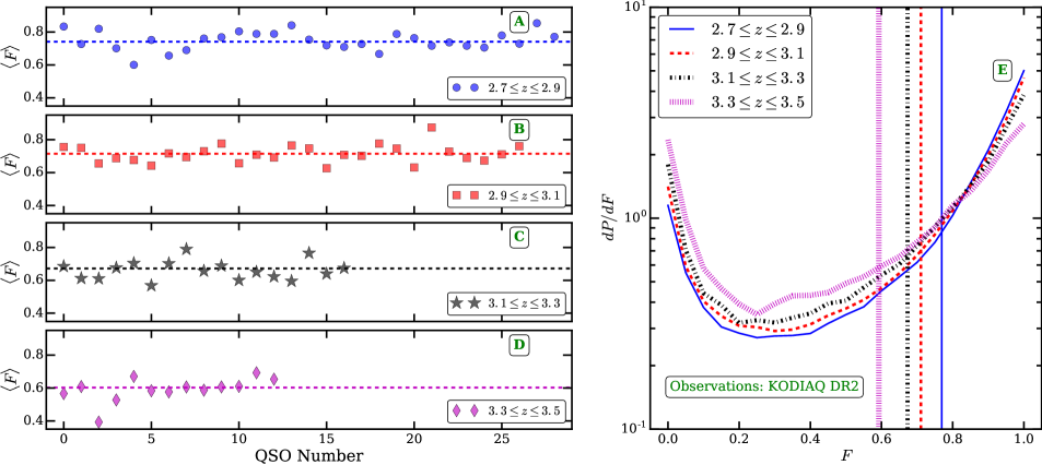
In this section we test if the observed excess in mean flux at in the kodiaq dr2 sample is due to the presence of any unusual QSO sightlines. To check if there are any outliers in this particular redshift bin, we plot the mean flux along individual sightlines in Fig. 21 for four redshift bins. Fig. 21 illustrates that the distribution of mean flux along sightlines is random around the mean flux (dashed line in panel A to D) of the entire sample for all redshift bins. We also do not see any outlier at . Since the mean flux along a sightline is an average quantity, we also check if there is any significant deviation in the observed FPDF evolution in panel E of Fig. 21. The observed FPDF at also does not show any unusual deviation from other redshift bins. The excess in at may thus be real in the kodiaq dr2 sample. Another reason for the excess could be that the number of sightlines at are limited in our sample. Our preliminary analysis using UVES squad dr1 (Murphy et al., 2019) while showing distinct change in the slope at z does not show any prominent excess. We plan to investigate this further in our future work. However, we emphasize that the effect of excess in at has a marginal effect on our measurements of thermal parameters. This is because for any thermal parameter variation we rescale the optical depth in our simulations to match the mean flux. Thus, even if there are any systematics in the evolution in the kodiaq dr2 sample, this does not significantly change the main results of this work.
Appendix C Comparison of observed flux statistics errors
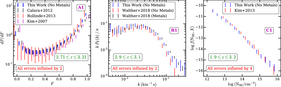
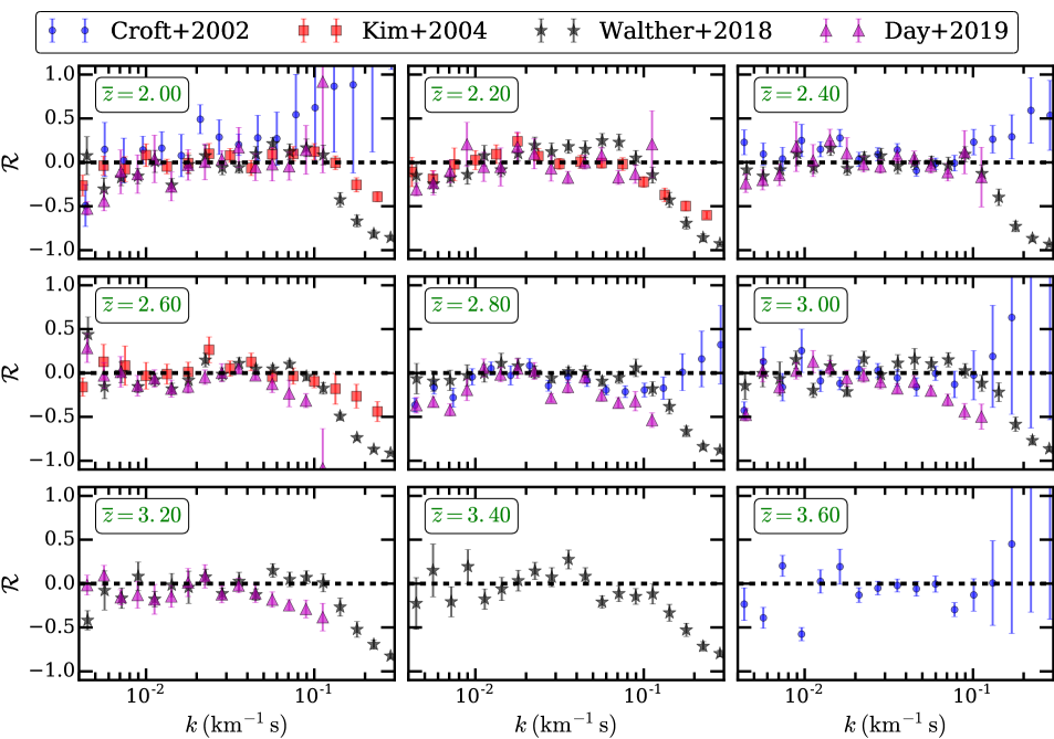
In §2.1 we discuss the consistency of observed flux statistics from this work with that in the literature. In this section, we compare the errors of the observed FPDF, FPS and CDDF from this work with measurements in the literature. The errors for observed statistics are normally determined using the bootstrap method (except in Rollinde et al., 2013). For a fair comparison, we also compute the errors using the bootstrap method. Fig. 22 shows a comparison of the errors for different statistics. In general, the errors in different statistics from this work are either consistent or slightly smaller than those in the literature.
Panel A1 in Fig. 22 shows that the error in our observed FPDF is smaller than that in Kim et al. (2007); Calura et al. (2012); Rollinde et al. (2013). The smaller errors are due to the large number of QSOs in our sample. The large error in the FPDF of Rollinde et al. (2013) is due to the difference in their method of calculating the errors. Rollinde et al. (2013) argue that the errors computed using the bootstrap method are underestimated and may not account for the cosmic variance accurately. Hence they derive the errors from large number of simulated mocks. Furthermore, their sample size was limited to at the redshift of interest. We have calculated the errors on our other observed statistics using both methods and accounted for cosmic variance (see §4.2 for details).
Panel B1 in Fig. 22 shows a comparison of the error of the FPS from this work with that from Walther et al. (2018). The errors (for the no metal case) are similar in the two works. This is expected because the number of QSOs per redshift bin are similar in both cases. Similarly, the data quality is the same because the subsets of QSOs are both drawn from the kodiaq dr2 survey. The consistency in FPS and its error of this work with that from Walther et al. (2018) reflects the consistency of both the data and our method of calculating the FPS. This consistency is important because the FPS is one of the statistics used in this work to measure thermal parameters.
In Fig. 23, we compare the observed FPS measurements from this work with those from Croft et al. (2002); Kim et al. (2004); Walther et al. (2018); Day et al. (2019). We find that our FPS measurements are generally in good agreement (maximum deviation is ) with those from the literature at . The large differences at are due to differences in the method of computing the FPS. In particular Kim et al. (2004); Walther et al. (2018) subtract power due to white noise in the spectra, whereas we do not subtract the noise power. Furthermore the number of observed spectra, quality of spectra (S/N) and total observed redshift path length is quite different in Croft et al. (2002); Kim et al. (2004) from that in our analysis. Even with such differences the FPS in these work seem to be in good agreement with our measurements. We also like to emphasize that any systematic differences in the method of computing the FPS does not significantly affect the measurements of thermal parameters. This is because we use the same method to compute the FPS statistics in simulations and observations.
In panel C1 of Fig. 22, we compare the errors of our CDDF with that from Kim et al. (2013). Kim et al. (2013) measured the CDDF from 18 high resolution high S/N (usually ) Ly forest spectra. On the other hand we measure the CDDF from a sample of high resolution but moderate S/N spectra. Thus the data size and data quality is different in both the works. These differences of the observed dataset are reflected in the CDDF errors. For example the errors in our CDDF at is larger than that from Kim et al. (2013). This is because low systems are affected more by the S/N of the spectra. Since S/N of our sample is smaller than in Kim et al. (2013), our CDDF error at small is correspondingly large. At high , S/N is no longer an issue since lines are detected with relatively high significance level. The errors in our CDDF at are smaller than that from Kim et al. (2013) because the number of spectra in our sample are nearly twice that in Kim et al. (2013). Even though there are differences in data quality and sample size, the CDDF and the associated errors from the two works are in good agreement with each other. The agreement between the CDDF demonstrates the consistency of viper in fitting the Ly forest with Voigt profiles. This consistency is important because we use the parameter of Voigt profile fits to constrain thermal parameters. In summary, the observed statistics with associated errors from this work are in good agreement with that from the literature.
Appendix D Variation in thermal parameters
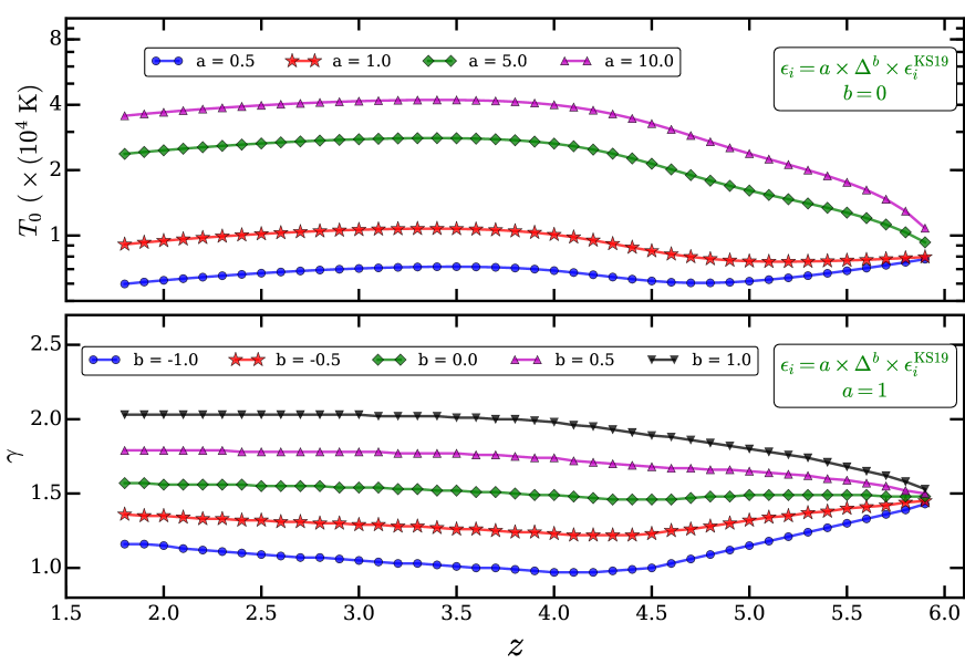
In this section, we explain our method of generating different thermal histories for a given UVB model. We vary the thermal parameter evolution by modifying the H i, He i and He ii photo-heating rates of the KS19 UVB. Following the approach of Becker et al. (2011), we scale the photo-heating rates () by two free parameters such that where [ H i, He i, He ii ]. A change in factor () leads to variation in () while keeping the evolution of () relatively unchanged. It is important to note that the variation in thermal parameters obtained by scaling the photo-heating rate is not physical. Ideally, one would like to vary the properties of the ionizing sources such as, luminosity function, QSO SED index, redshift of reionization etc., and generate the UVB model from a cosmological 1D radiative transfer code. However, such an approach cannot produce a large variation in and (but see Oñorbe et al., 2019). Our approach, even though not physical, is useful in practice to probe a large range of the parameters and on a finely sampled grid. Fig. 24 shows examples of the evolution in and obtained by varying and for several thermal histories. The case and shows the and evolution obtained using the default photo-heating rates from the KS19 UVB. Note that the shock heated gas ( K) is mostly unaffected by the photo-heating rate scaling, while the low density gas responds to this scaling differently and changes normalization () and slope () of the TDR.
When measuring the thermal parameters, it is important to sample the plane densely enough. A coarse sampling of plane can lead to incorrect best fit values and excessive smoothing of the field which, in turn, can result in underestimation of the uncertainties of the thermal parameters. On the other hand a very dense sampling of would be computationally very expensive. We found it to be the best compromise to choose the grids such that is varied from K to K in steps of 500 K while is varied from to in steps of 0.05 at 777The corresponding and at other redshifts differ by percent. We have thus simulated the Ly forest for different thermal histories. The computational time required to run the thermal histories and extract mock spectra for 999 UVB models is million cpu hours.
Appendix E The sensitivity of Ly forest statistics to ,
E.1 Kernel Density Estimation
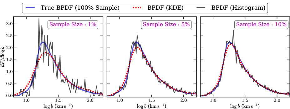
Kernel density estimation is a non-parametric method to estimate the probability distribution function. KDEs are a generalization of histograms with the advantage that the loss of information due to binning of the data is minimal with the KDE method. Unlike histograms, KDE is not sensitive to the choice of bins. The PDF calculated using the KDE method converges faster than the simple histogram method.
We use KDE to estimate the PDF of wavelet amplitudes, curvature and parameters. There are 3 main reasons for using KDE instead of histograms (i) the number of observed sightlines per redshift bins are usually limited (ii) the observed spectra have finite S/N and (iii) characterizing the shape of the PDF is important as it is sensitive to thermal and ionization parameters.
When calculating PDFs with KDE, we chose a Gaussian function as a kernel. The bandwidth () of the kernel is set by Scott’s rule, , where is the variance of the quantity whose PDF is to be estimated and is number of samples. Fig. 25 illustrates the advantage of using KDE over histograms to estimate the distribution (BPDF) from one of our models. First we generate a true BPDF by fitting Voigt profiles to 500 sightlines. We then randomly chose a fraction of sightlines and estimate the BPDF using histograms and KDE. The left, middle and right panel in Fig. 25 show the comparison of the BPDF using the histogram and KDE methods for 1%, 5% and 10% of the total sample. Fig. 25 clearly demonstrates that with KDE the estimated BPDF reaches a good approximation of the the true BPDF with a smaller sample than with the histogram method. PDFs estimated using KDE are smoother and converge faster than PDFs estimated with the histogram method888The bin center and bin width is fixed in Fig. 25. One can use coarse binning with the histogram method to estimate PDFs. However, the coarse binning can lead to loss of information with regard to the detailed shape of the PDF..
Appendix F Resolution and Convergence Tests
The size of the simulation box used in this work (L10N512) is 10 Mpc/h and is likely to be smaller than the typical size of He iii bubbles. As discussed in §3 the choice of our simulation box is motivated by the trade-off between dynamic range needed to resolve the Ly forest at and the large thermal parameter space to probe. However, it is important to demonstrate the sufficient convergence of our simulation by comparing the properties of the Ly forest from this work with that from a range of simulations in which box sizes and particle numbers are varied. We illustrate the convergence of our simulation in Fig. 26 to 31. We compare the FPDF, FPS, curvature PDF, wavelet PDF, BPDF and CDDF statistics from our model with that from the Sherwood simulation suite Bolton et al. (2017) at . For a fair comparison we chose thermal parameter consistent with that from the Sherwood simulations. For the models shown in Fig. 26 and 27, we post-process the simulated spectra to match the observed properties of our sample at . Note that the initial conditions of the density field used for the L10N512 simulation in this work is different from those used in the Sherwood simulation suite. When we rescale the optical depth to match the mean flux, we find that the amount of rescaling required is very similar in all the models. Fig. 26 to 31 shows a good agreement between our model statistics with that from the L10N512 Sherwood simulation suggesting that our method of varying the thermal history is consistent with the self-consistent gadget-3 simulation. The slight mismatch between our Ly forest statistics and that from the Sherwood simulation suite are primarily due to cite and not due to differences in initial conditions or the UVB models used. In Gaikwad et al. (2018), we have shown this explictly by comparing the Ly forest statistics from spectra post-processed with cite and those from self-consistent simulations for the same initial condition and UVB model. However, these differences are smaller than the observational uncertainties and are compensated by the ability of our method to probe the large thermal parameter space which would be computationally expensive for simulations with larger dynamic range/particle numbers. Fig. 27, 29 and 31 also illustrate that the statistics are converged with regards to box sizes. We compare the statistics from the L10N512, L20N512, L40N1024 and L80N2048 Sherwood simulations. The good agreement among the Sherwood models L40N512, L40N1024 and L40N2048 (Sherwood) indicates that the statistics are converged with regard to resolution/ particle mass.
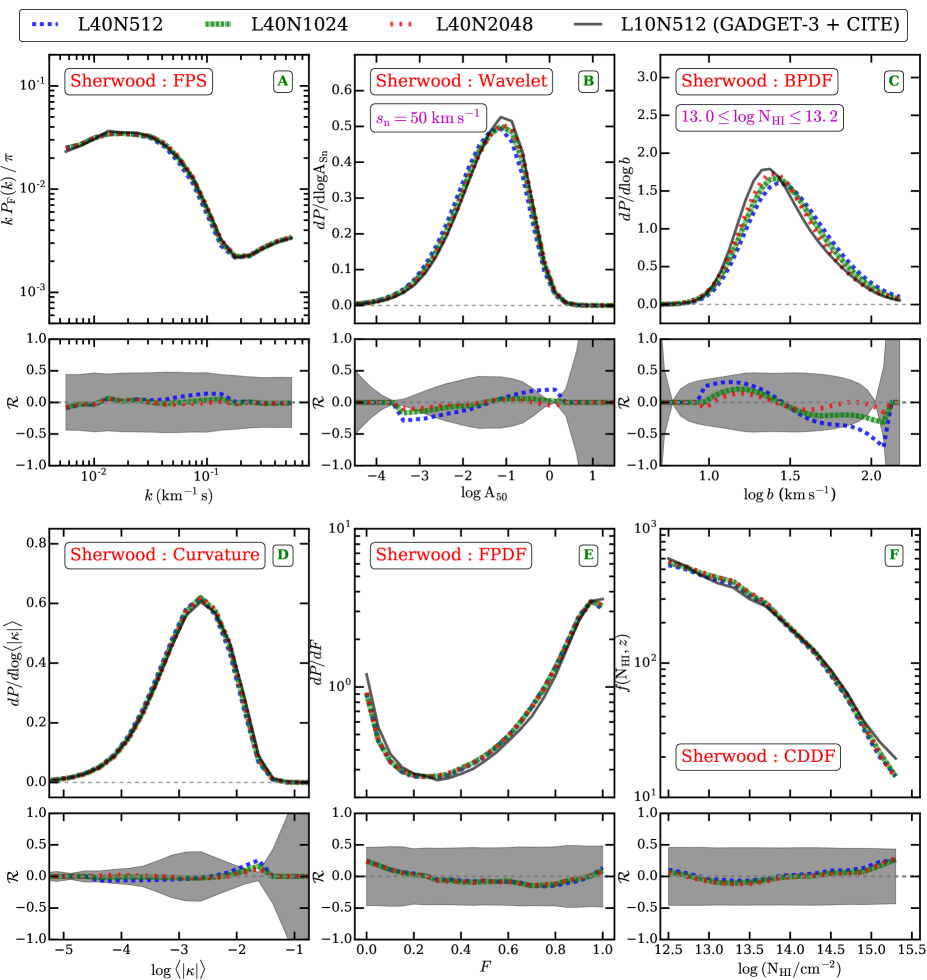
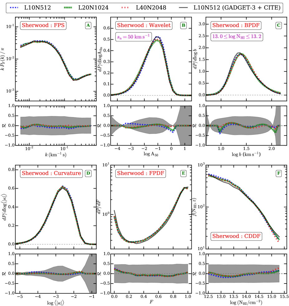
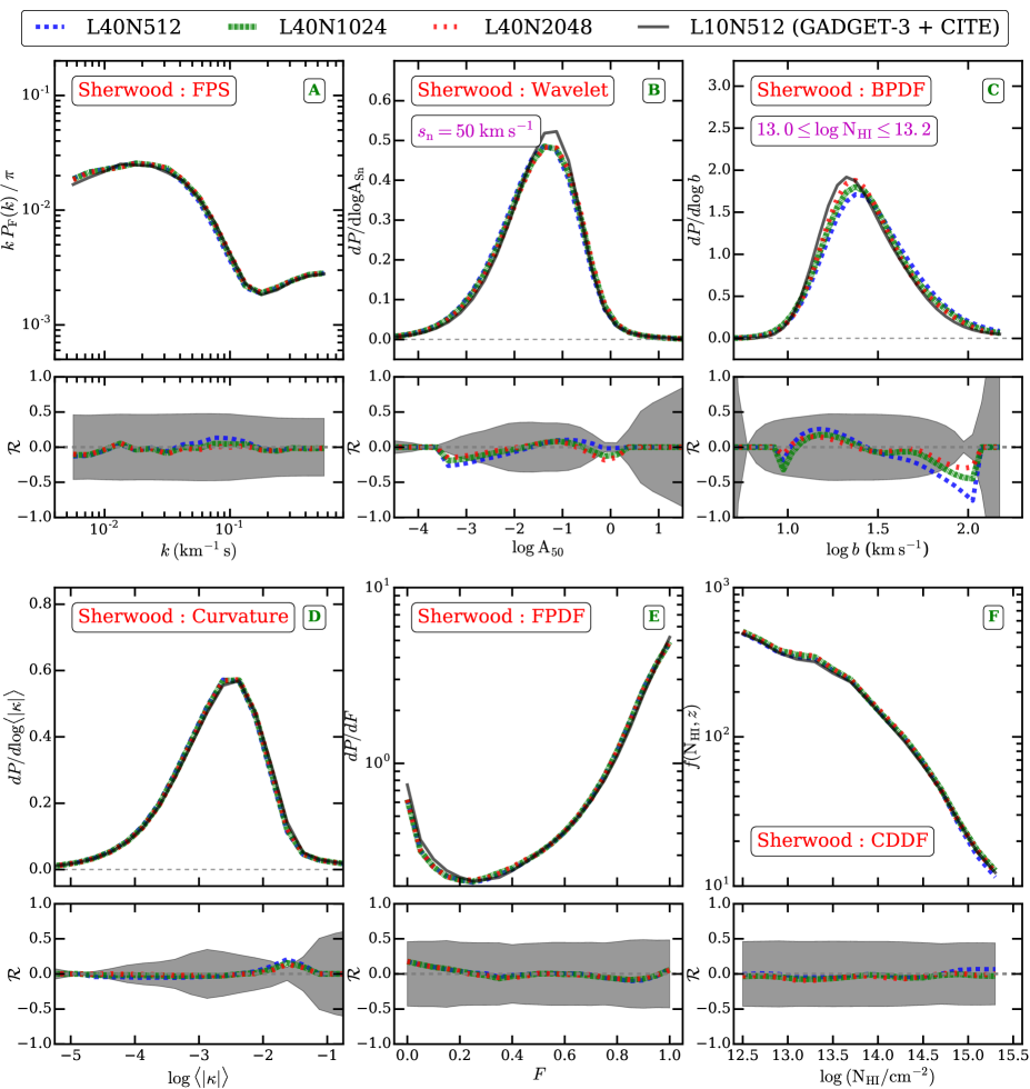
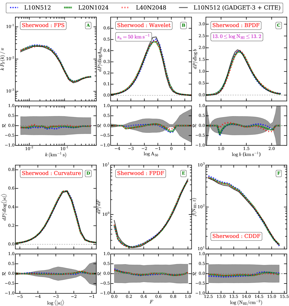
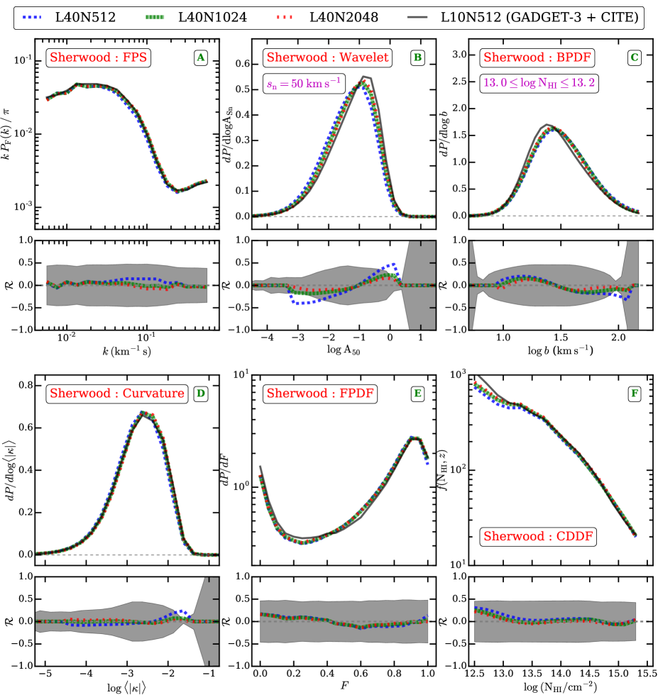
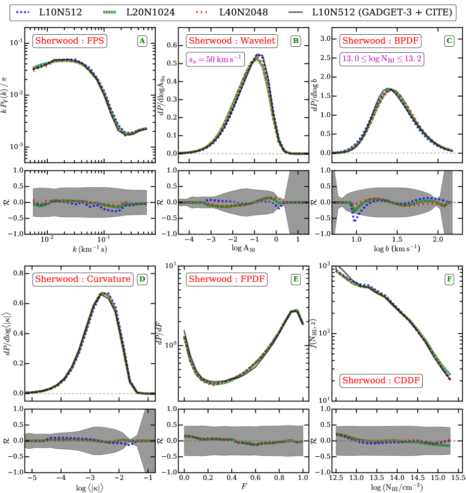
Appendix G Comparison of best fit statistics with observations
| Redshift | distribution[a] | Flux power spectrum | Wavelet PDF[b] | Curvature PDF | Joint Analysis |
|---|---|---|---|---|---|
| 2.0 0.1 | 1.45 | 1.15 | 1.70 | 1.51 | 1.50 |
| 2.2 0.1 | 1.51 | 1.33 | 1.80 | 1.43 | 1.57 |
| 2.4 0.1 | 1.85 | 1.75 | 1.17 | 1.64 | 1.34 |
| 2.6 0.1 | 1.02 | 0.85 | 1.94 | 1.78 | 1.40 |
| 2.8 0.1 | 1.77 | 1.61 | 1.01 | 0.45 | 1.21 |
| 3.0 0.1 | 1.35 | 0.71 | 1.29 | 0.92 | 1.10 |
| 3.2 0.1 | 1.53 | 0.87 | 1.23 | 1.29 | 1.24 |
| 3.4 0.1 | 1.45 | 0.71 | 1.45 | 0.69 | 1.12 |
| 3.6 0.1 | 1.61 | 0.60 | 0.54 | 0.82 | 0.94 |
| 3.8 0.1 | 1.72 | 0.73 | 0.72 | 1.23 | 1.14 |
-
a
The reduced is calculated by adding the between model and data distribution in different bins.
-
a
The reduced is calculated by adding the between model and data wavelet PDF for different wavelet scales ().
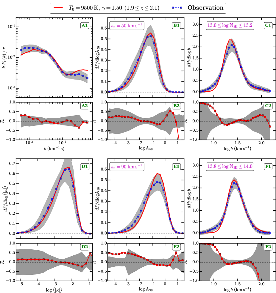
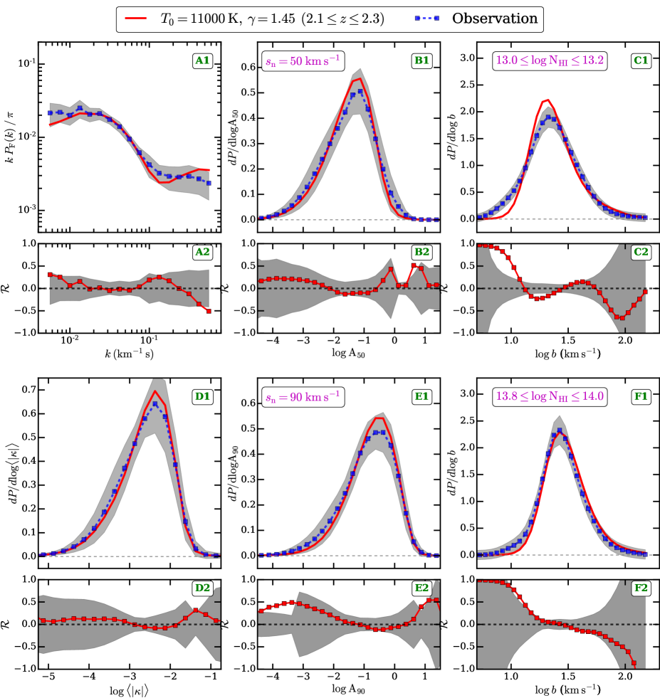
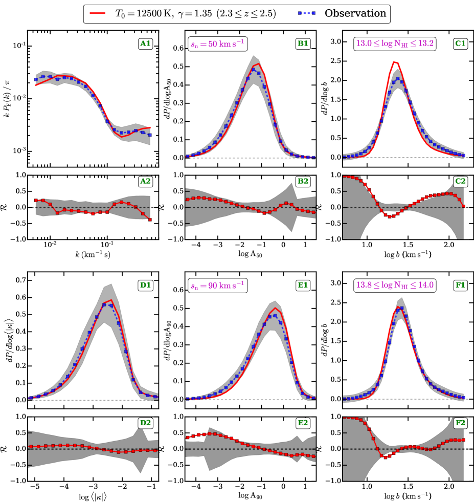

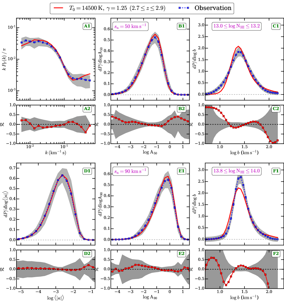
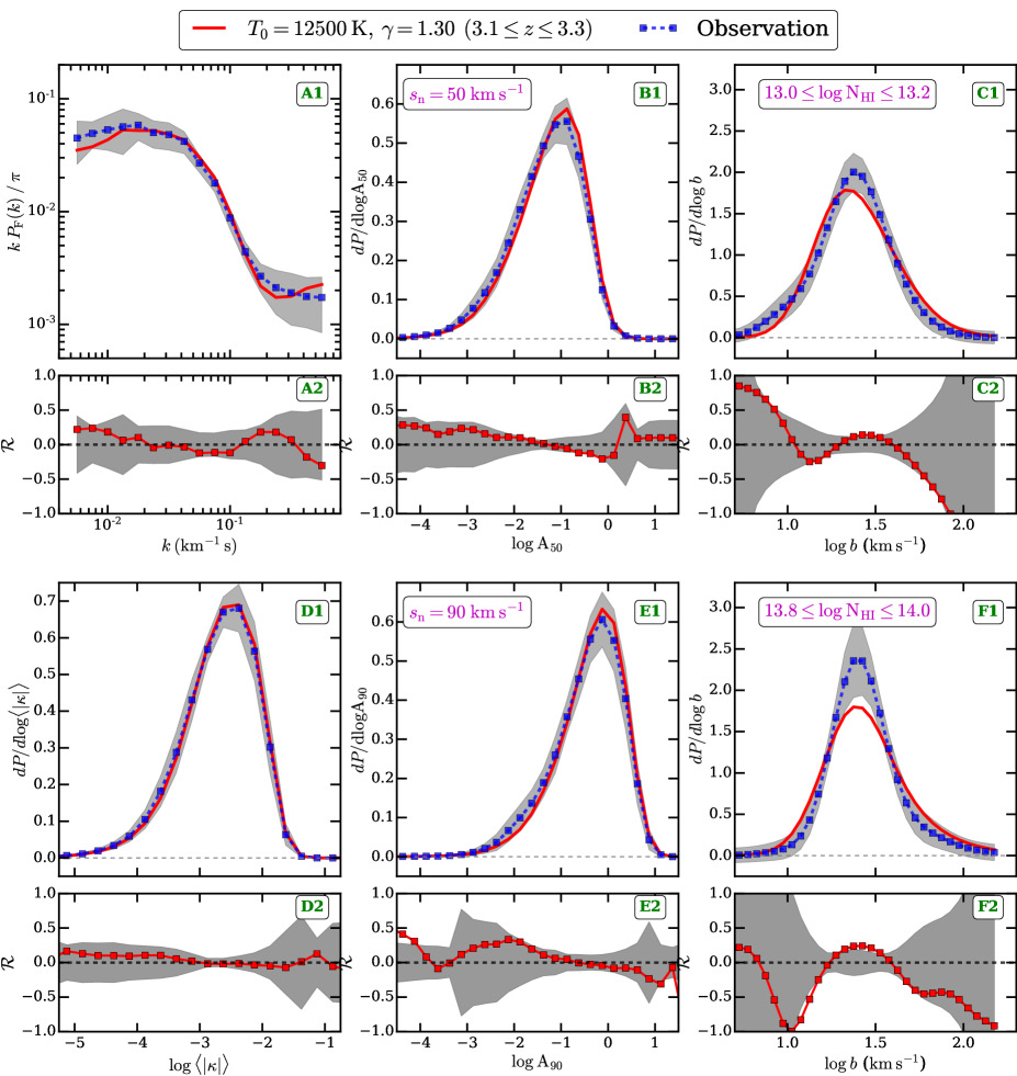
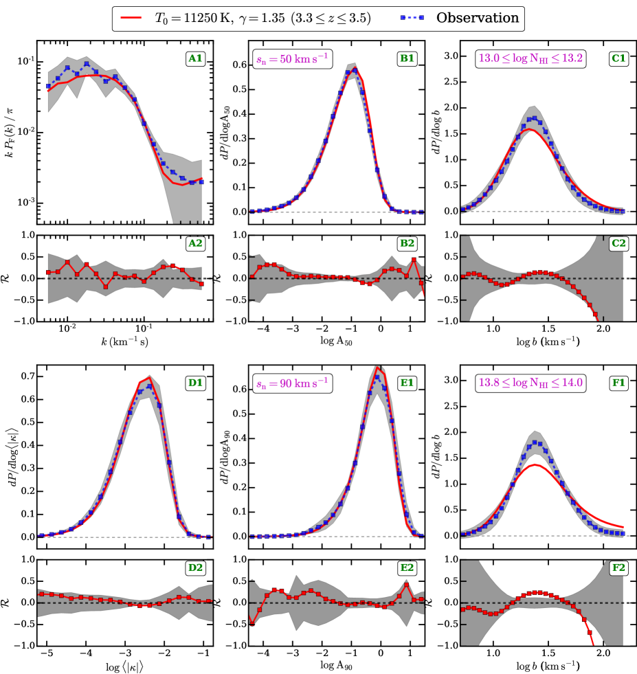
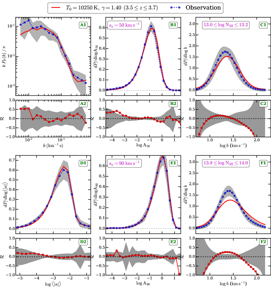
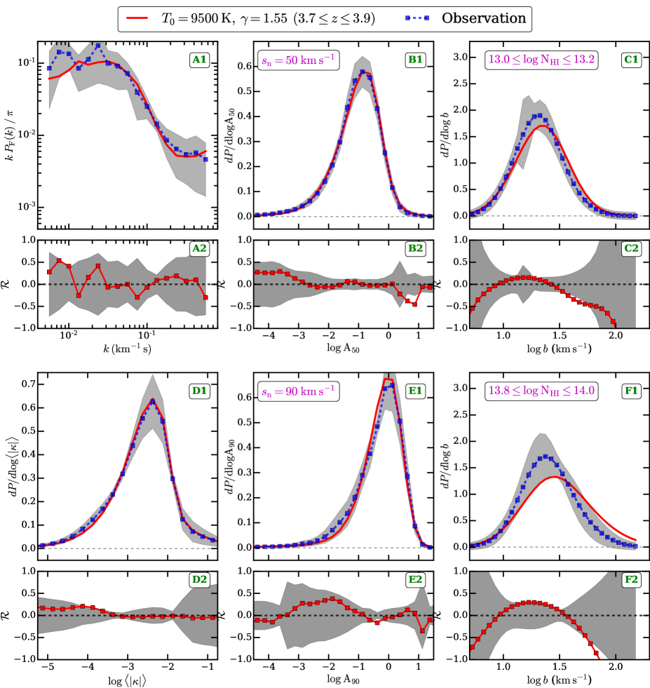
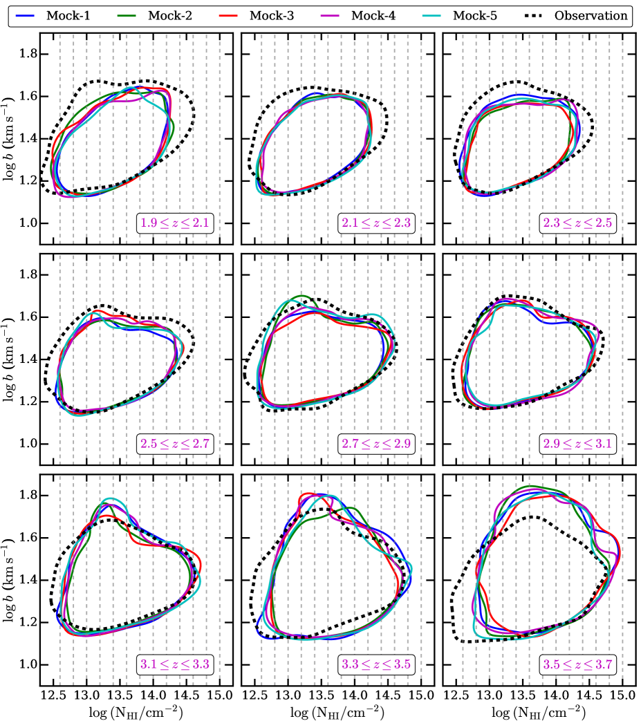
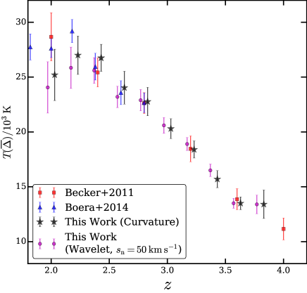
Similarly to Fig. 12, we show the comparison of FPS, wavelet, BPDF and curvature statistics of our best fit models with those obtained from observations at different redshift bins in Fig. 32 to 40. In general, the predictions of the best fit models are in good agreement with the observed statistics. We summarize the reduced between best fit model and observations in Table 5. The reduced is close to 1 in most cases.
We also plot a comparison of the observed contours (that includes 90 percent of points) with that from 5 mock samples (out of 100) in Fig. 41. The mock distribution corresponds to the best fit thermal parameters model. Traditionally, the lower envelope in the distribution is used to measure the thermal parameters. The limitations of this method are described in §4.1.4. Fig. 41 shows that the 2D observed distribution is similar to that from the mock samples at all redshifts. However, in general we see a mismatch between observed and best fit distribution at low and high . The low systems are usually contaminated due to the finite S/N of the spectra. Note here that the Voigt decomposition of high systems may not be unique. This effect is more prominent at higher () redshifts. Due to combination of these effects the mock distributions further show some differences compared to observations. It is noteworthy that the shape of the contours for lower values from the simulations are in good agreement with that from observations. The variations in the distribution in different mock samples is also small indicating that the distribution is converged with respect to cosmic variance. In summary, the distribution from our best fit models is in general good agreement with that from observations.
In Fig. 16 (panel B1), we show a comparison of from our method using the characteristic density with the results from Becker et al. (2011); Boera et al. (2014). To get the evolution in our model we assume the best fit evolution (with errors). To perform a fair comparison with the Becker et al. (2011); Boera et al. (2014) method, we show the temperature at the characteristic density from our work and Becker et al. (2011); Boera et al. (2014) in Fig. 42. Our temperature measurements from the curvature and wavelet statistics are in good agreement with that from the literature at . However, our measurements at are systematically lower than that from the literature, but are still consistent within . It is interesting to note that the characteristic density predicted from our model ( ) is also smaller at compared to that from Becker et al. (2011, ).
Appendix H Sources of uncertainty in , measurements
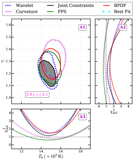

In addition to statistical uncertainty, the , measurements are also affected by the modeling and observational uncertainties. We have considered four main sources of uncertainties contributing to the total uncertainty on the measured parameters. These are uncertainties due to (i) continuum placement, (ii) contamination by unidentified metal lines, (iii) (numerical) modeling and (iv) cosmological parameters. The first two uncertainties are observational uncertainties while the later two uncertainties are modeling uncertainties. We discuss below the contribution of each to the measurement uncertainty in detail.
| Redshift | Statistical | Model | Cosmological | Metal line | Continuum | Best fit Total |
| uncertainty [a] | uncertainty [b] | parameters [c] | contamination [d] | uncertainty [e] | uncertainty [f] | |
| Contribution of various uncertainties to the total uncertainty on (in K) measurements | ||||||
| 2.0 0.1 | 1254 | 285 | 31 | 125 | 100 | 9500 1393 |
| 2.2 0.1 | 831 | 330 | 36 | 125 | 125 | 11000 1028 |
| 2.4 0.1 | 952 | 382 | 41 | 100 | 100 | 12750 1132 |
| 2.6 0.1 | 894 | 405 | 44 | 125 | 400 | 13500 1390 |
| 2.8 0.1 | 848 | 442 | 48 | 125 | 375 | 14750 1341 |
| 3.0 0.1 | 827 | 442 | 48 | 125 | 375 | 14750 1322 |
| 3.2 0.1 | 1045 | 382 | 41 | 100 | 375 | 12750 1493 |
| 3.4 0.1 | 796 | 338 | 37 | 125 | 250 | 11250 1125 |
| 3.6 0.1 | 885 | 308 | 33 | 125 | 125 | 10250 1070 |
| 3.8 0.1 | 690 | 278 | 30 | 100 | 125 | 9250 876 |
| Contribution of various uncertainties to the total uncertainty on measurements | ||||||
| 2.0 0.1 | 0.081 | 0.018 | 0.003 | 0.010 | 0.012 | 1.500 0.096 |
| 2.2 0.1 | 0.080 | 0.017 | 0.003 | 0.013 | 0.050 | 1.425 0.133 |
| 2.4 0.1 | 0.095 | 0.016 | 0.003 | 0.010 | 0.025 | 1.325 0.122 |
| 2.6 0.1 | 0.092 | 0.015 | 0.003 | 0.025 | 0.025 | 1.275 0.122 |
| 2.8 0.1 | 0.094 | 0.015 | 0.003 | 0.010 | 0.012 | 1.250 0.109 |
| 3.0 0.1 | 0.106 | 0.015 | 0.003 | 0.013 | 0.012 | 1.225 0.120 |
| 3.2 0.1 | 0.115 | 0.015 | 0.003 | 0.013 | 0.013 | 1.275 0.129 |
| 3.4 0.1 | 0.096 | 0.016 | 0.003 | 0.012 | 0.010 | 1.350 0.108 |
| 3.6 0.1 | 0.088 | 0.017 | 0.003 | 0.012 | 0.010 | 1.400 0.101 |
| 3.8 0.1 | 0.066 | 0.018 | 0.003 | 0.038 | 0.062 | 1.525 0.140 |
-
a
Statistical uncertainty corresponds to uncertainty from joint constraints of respective parameters.
-
b
Model uncertainty corresponds to uncertainty in modeling of the Ly forest in our simulation.
-
c
Cosmological parameter uncertainty is calculated using the Gunn-Peterson approximation. Note that the GP approximation does not account for the uncertainty in .
-
d
Contribution of unidentified metal lines to the uncertainty in derived quantity.
-
e
Continuum placement uncertainty () is assumed to be percent. For and measurements, includes the uncertainty due to the mean transmitted flux for a given continuum. For measurements, include the uncertainty due to variation of and parameters.
-
f
Total uncertainty is obtained by
H.1 Continuum placement uncertainty
When comparing simulated Ly forest spectra with observations, it is customary to use normalized observed spectra (). The continuum fitting of spectra is usually based on high order polynomial fitting connecting points in the spectrum believed to have no absorption. The uncertainty in continuum placement affects the observed flux statistics of Ly forest data and influences the inferred physical parameters. In the kodiaq DR2 sample, all the spectra are normalized by the procedure described in O’Meara et al. (2015, 2017). The continuum placement uncertainty in the kodiaq DR2 sample is of the order of a few percent (see O’Meara et al., 2015). We assume a conservative value for the continuum placement uncertainty of percent. If is the flux corresponding to the default continuum and is the uncertainty in continuum placement then we define a low /high continuum as .
We quantify the effect of continuum placement uncertainty by rescaling the observed flux, deriving all the statistics from the rescaled spectra and constraining the , parameters using our simulations. Fig. 15 shows the effect of continuum placement on the (joint) and constraints. For low (high) continuum placement, and are systematically underpredicted (overpredicted) relative to measurements with the default continuum. One can qualitatively understand this systematic effect of continuum placement on flux. Since dividing a flux by a low (high) continuum stretches (compresses) the flux in the vertical direction, this artificially reduces (increases) the line widths and hence one gets systematically smaller (higher) temperature. Fig. 44 shows a similar effect of continuum placement uncertainty in the other redshift bins. The uncertainty in and measurement due to continuum placement is systematic in nature hence we add this uncertainty in the total error budget (see Table 6).
H.2 Metal line contamination uncertainty
The observed Ly forest is usually contaminated by absorption lines arising from metals. For a given temperature, the metal lines are typically narrower than H i lines because for thermally broadened lines, the line width and is larger for metals than hydrogen. The presence of such narrower metal lines can potentially bias the temperature measurement to lower values. In this work, we do not model the intergalactic metal absorption systems as our simulations neither follow chemical evolution of metals nor include feedback processes. To mitigate this, we chose QSO sightlines that do not contain DLAs or sub-DLAs. Thus our sample selection criteria minimizes the number of metal lines contaminating the Ly forest. Furthermore, we identify metal lines and replace them with continuum and add noise. We use manual and automated approaches to identify metal lines. We find that both approaches give consistent results.
In the manual approach, we first find the redshift of absorption systems using part of the spectra redward of the H i emission line. Corresponding to this redshift, we look for other transitions contaminating Ly forest. Due to insufficient wavelength coverage, it is possible that we may not identify all the metal lines. Hence we manually look at each spectrum and look for obvious metal line systems. We then replace metal lines with continuum and add noise 999We account for the effect of metal lines blended with H i absorption lines..
The manual method is tedious and somewhat subjective. Hence, we have also used an automatic method to identify the metal lines based on line widths. Since metal lines are narrower than corresponding H i lines, we fit all the spectra with multi-component Voigt profiles using viper. We treat all the lines with km s-1 as metal lines101010The narrowest line that can be detected in spectra is limited by the line spread function (FWHM km s-1) of the spectrograph.. We replace these metal lines with continuum and add noise accounting for any blending effects.
Fig. 15 and Fig. 44 shows the effect of metal contamination on and constraints in all the redshift bins. As expected, when we use flux statistics for the observed spectra without subtracting metal contamination, we get systematically smaller and . Even though we identify and remove the metal lines, it is still possible that some of the metal lines are not identified by our method. Since the metal lines contamination introduces an uncertainty of percent, we add this uncertainty in the total error budget of constrained parameters (see Table 6).
H.3 Cosmological parameter uncertainty
All the results presented in this work assume a flat CDM cosmology consistent with Planck Collaboration et al. (2014). However the Ly optical depth depends on cosmological parameters and as
| (7) |
where we assume that recombination rate scales with temperature as . It would be computationally expensive to perform all the analysis with varying cosmological parameters. Hence we use a simplified approach of propagating the error using the above equation. For this we use the uncertainty on and from Planck Collaboration et al. (2014). The cosmological parameters derived from the CMB are correlated with each other. Some of these correlation may lead to a cancellation of errors. However, while performing the error analysis, we always add errors due to different cosmological parameters. Thus the assumed uncertainty due to cosmological parameters is conservative. We do not account for the uncertainty in and as this would require to perform self-consistent gadget-3 simulations. However it is important to note that, we find that the uncertainty in and measurements due to cosmological parameters uncertainty is small, percent (see Table 6).
H.4 Modeling uncertainty due to Jeans smoothing
In the simulations, we vary the thermal state of the IGM by post-processing gadget-3 simulations using cite. Pressure smoothing effects due to the hydrodynamical response of the gas are important during reionization (Park et al., 2016; D’Aloisio et al., 2020). As shown in Gaikwad et al. (2018), we account for the pressure smoothing of the gas by convolving the SPH kernel with a Gaussian kernel that depends on the pressure smoothing scale (Gnedin & Hui, 1998; Kulkarni et al., 2015). This approach is based on the ansatz that the Ly absorbers are in local hydrostatistic equilibrium (Schaye, 2001). However, this assumption may not be valid during the process of reionization as the photo-heating time scales are typically shorter than the dynamical response time of the gas. In addition to this, the Ly forest traces the neutral gas in large scale filaments which are undergoing gravitational collapse onto nearby over-dense objects. The hydrostatic equilibrium approximation may thus not be correct. To quantify the effect of this ansatz, we perform a self-consistent gadget-3 simulation with enhanced photo-heating rates where is doubled. The dynamical effect of pressure smoothing is thus captured accurately in this self-consistent simulation. We compute the Ly forest statistics for this self-consistent model and assume it as the fiducial model. We constrain , and using our model, i.e. gadget-3 (at lower temperature) + cite (with convolution of SPH kernel with Gaussian). We find that the fiducial , and are recovered within 2.5, 1.3 and 0.6 percent. Such a good level of agreement is partly expected because the smoothing of transmitted flux at these redshifts is dominated by temperature, while the pressure smoothing effects are sub-dominant. We account for this modeling uncertainty in the total error budget of derived parameters (see Table 6). We also refer the reader to §3 for a related discussion.
Appendix I Thermal parameter evolution in UVB models
In this section we discuss the effect of uncertainty in observed and modeling parameters in the UVB models on the thermal parameter evolution during He ii reionization.
I.1 Effect of uncertainty in at on thermal parameter evolution at
In this section we discuss the effect of varying the thermal parameters and at (the initial redshift chosen for cite in this work) on the thermal evolution at . Recently Gaikwad et al. (2020) measured () at and found it to be larger than predicted by the \al@haardt2012,onorbe2017,khaire2019a,faucher2020; \al@haardt2012,onorbe2017,khaire2019a,faucher2020; \al@haardt2012,onorbe2017,khaire2019a,faucher2020; \al@haardt2012,onorbe2017,khaire2019a,faucher2020 UVB models. Since we run cite from to , it is possible that an uncertainty in and at affects the thermal parameter evolution at . Fig. 45 shows that the effect of even a large uncertainty in thermal parameters at is subdominant at lower redshifts. This is because the lower redshift thermal evolution is mainly affected by the He ii reionization prescriptions used in these models. Thus the effect of uncertainty in at is less than 4 percent (maximum) at . Note that even though we show this result only for the FG20 UVB models, the results are similar for the other UVB models.
I.2 Effect of QSO spectral energy distribution on thermal parameter evolution at
The observed QSO spectral index (, ) is another uncertain quantity in UVB calculations. The observations of stacked QSO spectra in the far ultra-violet suggests that QSO spectral indices vary from to (Lusso et al., 2014; Stevans et al., 2014; Shull & Danforth, 2020). Recently Gaikwad et al. (2019) showed that the effect of the QSO spectral index on thermal parameter evolution is degenerate with the redshift of He ii reionization in KS19 such that a flatter QSO SED corresponds to an earlier He ii reionization. They further showed that is consistent with the evolution of from Worseck et al. (2019). In Fig. 47, we show the comparison of our thermal parameter measurements with that predicted by the KS19 UVB for different QSO spectral indices. Irrespective of the QSO spectral index, the total emissivity is kept constant in all the models. The shape of the thermal parameter evolution is hence similar for all the models. The redshift of maximum occurs at slightly higher redshift and is slightly higher for flatter (small ) QSO SED. The earlier temperature rise is mainly because of the evolution (see panel B1 Fig. 47) in these models which is also different such that He ii reionization occurs slightly earlier for flatter QSO SED (Gaikwad et al., 2019). However, even after changing the QSO SED spectral index in the observationally allowed range, the thermal parameter evolution in the KS19 UVB model is significantly different from our measurements. This suggests that additional modifications (such as evolution) may be needed for the KS19 UVB models to become consistent with our temperature measurements.
I.3 Modifications to UVB models
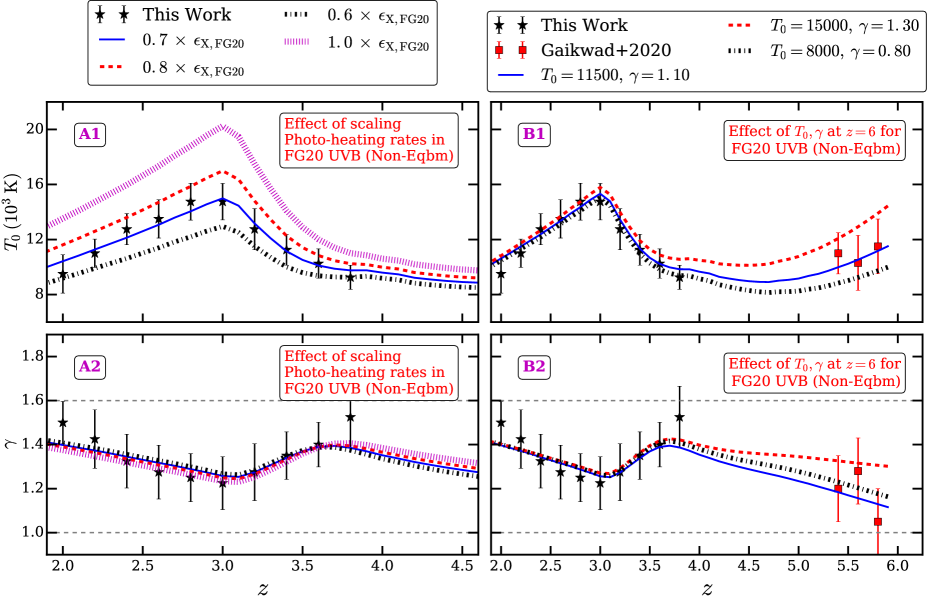
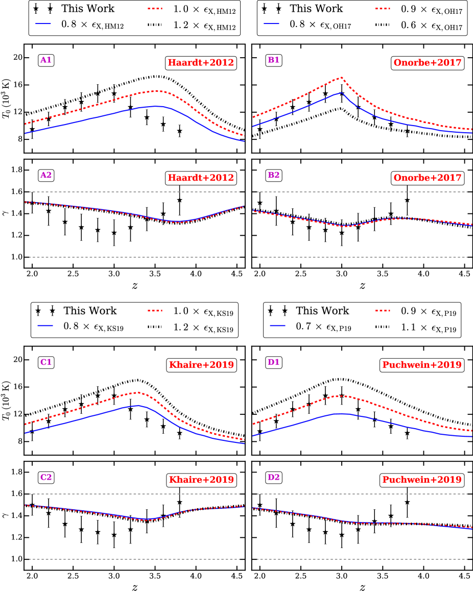
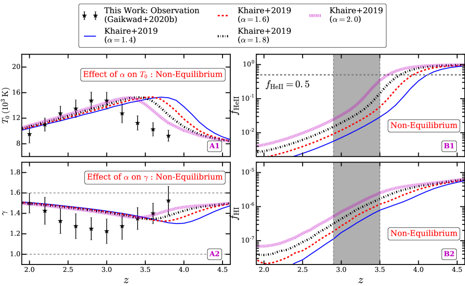
Recently FG20 updated their Faucher-Giguère et al. (2008) UVB model with updated constraints on galaxy and AGN luminosity functions (Kulkarni et al., 2019), intergalactic H i and He ii opacity models, and calibrations to measurements of and etc. In their UVB model, AGN (galaxy) dominate the H i ionizing background at (). Their UVB model crucially depends on parameters related to the reionization history mainly the total temperature increments due to H i () and He ii () reionization heating. The H i and He ii photo-heating rates are directly proportional to and respectively. Since the timing and amount of photo-heating during He ii reionization is poorly constrained at present, they parameterize this ignorance in and . \al@onorbe2017,faucher2020; \al@onorbe2017,faucher2020 assumed K and K and obtain a and evolution similar to previous measurements. However, both groups assumed that photo-ionization equilibrium is valid at all times. But as shown by Puchwein et al. (2015); Gaikwad et al. (2018); Puchwein et al. (2019), this is not a good assumption during He ii reionization as the photo-ionization time scales are shorter than the recombination time scales. Thus non-equilibrium ionization evolution is more physically motivated. Puchwein et al. (2015); Gaikwad et al. (2018) shows that the of the IGM in non-equilibrium is significantly larger than in equilibrium calculations. Thus when we use non-equilibrium ionization evolution for \al@onorbe2017,faucher2020; \al@onorbe2017,faucher2020 which are calibrated to match observation assuming photo-ionization equilibrium , we get significantly larger temperature predictions for their UVB models. In order to match the observations with non-equilibrium ionization evolution, we need to reduce and . The reduction of and by a factor of is equivalent to reducing H i, He i and He ii photo-heating rates by a factor .
Fig. 45 shows the variation in and evolution with the variation in and predicted by the FG20 model using gadget-3 + cite. We show results in Fig. 45 for four for H i, He i and He ii photo-heating rates. The main effect of changing this parameter is to reduce systematically at all redshifts while changes very little. This is expected as scaling the parameters , is equivalent to scaling H i and He ii photo-heating rates and such scaling changes (keeping relatively same see Fig. 24). Fig. 45 shows that the and evolution is consistent with our measurements if we use non-equilibrium ionization evolution with parameters in FG20. For completeness, we summarize the best fit and parameters used in \al@onorbe2017,faucher2020; \al@onorbe2017,faucher2020 in Table 7 that are consistent with our temperature measurements. In order to do a fair comparison with other UVB models, we show the and evolution for varying the photo-heating rates in Fig. 46. We find that other UVB models match the evolution in some redshift bins but are systematically above or below in other redshift bins. The evolution of is similar to that shown in Fig. 18.
Finally, we compare the evolution of and over the full redshift range and all the different flux statistics in Fig. 48. We emphasize that a considerable amount of work has also been done to measure the and evolution at . At these redshifts the thermal parameters have been measured using FPS Walther et al. (2019); Boera et al. (2019), curvature statistics Becker et al. (2011), proximity effects Bolton et al. (2012) and the width distribution of transmission spikes Gaikwad et al. (2020). These measurements broadly agree with the theoretical and evolution predicted by the different UVB models.
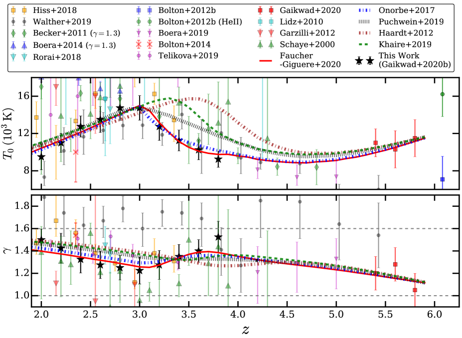
I.4 The way forward for UVB models
We have rescaled the photo-heating rates in §6.2 to better match our temperature measurements. Even though this is a simple modification to the UVB models, this is not necessarily physical because photo-ionization and photo-heating rates are ultimately linked to the population of ionising sources (QSOs and /or galaxies) and IGM properties. In this section we discuss the possible modifications that may be needed in the various UVB models to match our measurements. Note, however, that implementing these in the UVB models is beyond the scope of present work hence we discuss qualitative features of a physically motivated UVB model that could match our measurements.
From Fig. 18, it is clear that the maximum in occurs at systematically lower redshift than that from \al@haardt2012,khaire2019a; \al@haardt2012,khaire2019a UVB models. However, the maximum value of from these models seem to agree well with that from observations. This suggests that the normalization of the QSO emissivity in these models is roughly consistent with observations. However, the He ii reionization in these models starts early and is more gradual than suggested by observations (see panel B1 in Fig. 19). Thus, in \al@haardt2012,khaire2019a; \al@haardt2012,khaire2019a the redshift evolution of needs to be modified. In KS19, this could be achieved by changing the ratio of He ii and H i fractions (). Since there are only observational limits limits on and the fluctuations in He ii ionizing background are important at , there is scope for modification in the evolution of the KS19 UVB. The evolution can also be modified by varying QSO SED index ( Gaikwad et al., 2019). However, we show in online supplementary appendix I.3 that the observed thermal parameter evolution can not be matched by simply varying the QSO SED index within the observationally allowed range of (Lusso et al., 2014; Stevans et al., 2014; Shull & Danforth, 2020). For the HM12 UVB model both the QSO luminosity functions and QSO SED index need to be updated to be compatible with the most recent compilations of the relevant observation(see e.g. Kulkarni et al., 2019).
In summary, the observed thermal parameter evolution from this work suggests a combination of changes to existing UVB models. For \al@haardt2012,khaire2019a; \al@haardt2012,khaire2019a UVB models, modification in is necessary. For the \al@onorbe2017,puchwein2019,faucher2020; \al@onorbe2017,puchwein2019,faucher2020; \al@onorbe2017,puchwein2019,faucher2020 UVB models modification of the ionizing emissivity from QSOs is needed.
Appendix J Cumulative energy parameter
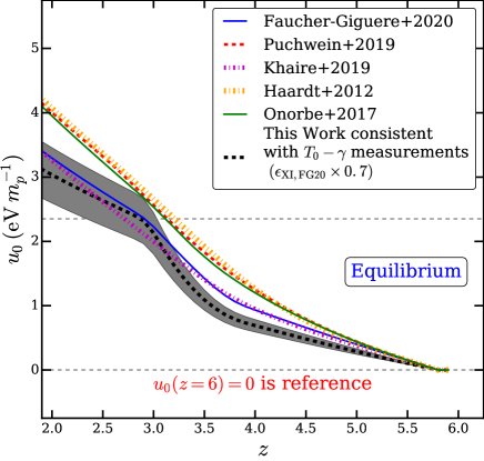
The default photo-heating rates of all the UVB models predict systematically higher than we measure at (see Fig. 18). Since we have changed the photo-heating rates to better match the observed evolution, it is also interesting to have a look at the evolution of the cumulative energy () deposited into IGM by He ii reionization. We calculate the cumulative energy per unit mass () deposited into IGM as
| (8) |
where (with XI H i, He i, He ii), are mean baryon density, Hubble constant, number density of species XI and photo-heating rate of specie XI (Nasir et al., 2016). To calculate for a simulation box with given UVB and at a given redshift, we first calculate the volume average neutral fraction . We then use above expression to compute . Given that there could be uncertainty in after H i reionization, we chose as a reference point. The defined in this work is mainly sensitive to heat deposited during He ii reionization.
In Fig. 49 we show the evolution of for all the UVB models with non-equilibrium ionization evolution. The observed evolution is difficult to measure directly from observations. To nevertheless facilitate a comparison, we show the evolution in Fig. 49 for the FG20 non-equilibrium UVB with scaled photo-heating rates that matches the observed evolution from this work. We treat the evolution corresponding to this model as that inferred from our temperature measurements (black dashed line with shaded region).
Fig. 49 also shows the evolution in all the UVB models assuming non-equilibrium ionization evolution. The photo-heating rates here are not scaled for the UVB models. At the predicted by all the UVB models is systematically higher than the evolution inferred from our temperature measurements (Table 4). Thus to match the observed evolution smaller values of energy deposited per unit mass at are required. It is interesting to note that at from the KS19 model is close to that from a model which is consistent with our measurements. However, the and evolution from the KS19 model is significantly different at . This is because accounts for the heating of the IGM, but does not account for the cooling of the IGM due to recombination, Hubble expansion or inverse Compton cooling etc. Hence to match the evolution, the whole of the evolution is important and not only matching at some redshift. The comparison of evolution in Fig. 49 again suggests that rather rapid He ii reionization is needed to match our measured evolution. The evolution in \al@haardt2012,khaire2019a,puchwein2019; \al@haardt2012,khaire2019a,puchwein2019; \al@haardt2012,khaire2019a,puchwein2019 is more gradual compared to the other two models.