Dynamical instability of minimal surfaces
at flat singular points

Abstract.

Suppose that a countably $n$-rectifiable set $\Gamma_{0}$ is the support of a multiplicity-one stationary varifold in $\mathbb{R}^{n+1}$ with a point admitting a flat tangent plane $T$ of density $Q\geq 2$. We prove that, under a suitable assumption on the decay rate of the blow-ups of $\Gamma_{0}$ towards $T$, there exists a non-constant Brakke flow starting with $\Gamma_{0}$. This shows non-uniqueness of Brakke flow under these conditions, and suggests that the stability of a stationary varifold with respect to mean curvature flow may be used to exclude the presence of flat singularities.

Keywords: mean curvature flow, varifolds, singularities of minimal surfaces.

AMS Math Subject Classification (2020): 53E10 (primary), 49Q05.

1. Introduction

A family of surfaces is said to move by mean curvature flow (abbreviated hereafter as MCF) if the velocity of motion is equal to the mean curvature at each point and time. The MCF is one of the simplest geometric evolution problems, and it has been studied intensively by numerous researchers over the last few decades. In the early stages of the development of the theory of MCF, Brakke introduced in [6] a notion of MCF - which is nowadays referred to as the Brakke flow - within the framework of geometric measure theory. It is a generalized notion of MCF where the evolving surfaces are not required to be classical, regular submanifolds, but rather varifolds, and where the classical parabolic PDE describing the evolution law is replaced by an ad hoc inequality which is adapted to the language of varifolds while still being able to capture the geometric features of MCF; see section 2 for a brief introduction to the subject, and [6, 20] for further references. The advantage of such a seemingly abstract approach is that it allows one to describe the evolution by mean curvature of singular surfaces (e.g. a moving network of curves in the plane with multiple junction points or a moving cluster of bubbles in the three-dimensional space), as well as to continue the evolution of classical surfaces also after singularities arise. At the same time, a possible drawback is that the solution to Brakke flow for a given initial datum may not be unique in general.

Recently, the authors of the present paper proved a general theorem concerning the existence of Brakke flow starting from any given closed countably $n$-rectifiable set $\Gamma_{0}$ in a strictly convex domain in $\mathbb{R}^{n+1}$ and with the additional property that the (topological) boundary of the evolving varifolds is fixed throughout the flow [19]. This existence result gives rise to a number of questions pertaining to the nature of the Brakke flow. One such question to be discussed in the present paper is the following:

$$\begin{split}&\mbox{Does there exist a \emph{stationary} initial datum $\Gamma_{0}$}\\ &\mbox{admitting a \emph{non-trivial} Brakke flow starting with it?}\end{split} \mathcal{Q}$$ ()

Here, “stationary” means that the first variation of the associated multiplicity one varifold vanishes, and “non-trivial” means that the flow is genuinely time-dependent: note that a stationary $\Gamma_{0}$ itself is a time-independent Brakke flow with no motion. Thus, the question is equivalent to inquiring about the non-uniqueness of Brakke flow starting from a given stationary $\Gamma_{0}$. To avoid instantaneous vanishing, it is also natural to require the continuity of the surface measures associated to the Brakke flow at $t=0+$. If $\Gamma_{0}$ is smooth, then one expects that all Brakke flows starting with it should be trivial, thus it is interesting to focus on stationary $\Gamma_{0}$ with singularities.

The main result of the paper is an affirmative answer to ($\mathcal{Q}$), and it can be roughly stated as follows (see Theorem 3.5 for the precise statement).

Theorem A.

Suppose that a closed countably $n$-rectifiable set $\Gamma_{0}$ is stationary, and that there exists $x_{0}\in\Gamma_{0}$ with the following properties:

• one of the tangent cones to $\Gamma_{0}$ at $x_{0}$ is a flat plane $T$ with multiplicity $Q\geq 2$, and

• the rescalings $(\Gamma_{0}-\{x_{0}\})/r$ locally converge to $T$ at a rate faster than $(\log(1/r))^{-1/2}$ as $r\rightarrow 0^{+}$.

Then, there exists a non-trivial Brakke flow starting from $\Gamma_{0}$.

We observe explicitly that the assumption (2) implies, in particular, that the varifold associated with the plane $T$ and carrying multiplicity $Q$ is the unique varifold tangent cone to $\Gamma_{0}$ at $x_{0}$. There is a plethora of examples of stationary $\Gamma_{0}$ admitting the kind of singularities described in (1) and (2): a typical candidate is any minimal immersion with a branched point; see Figure 1.

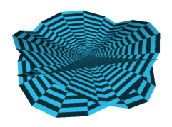
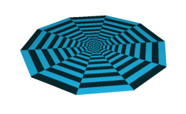
Figure 1. On the left, a minimal surface $\Gamma_{0}$ with a flat singularity of multiplicity $Q=3$. The homothetic rescalings $(\Gamma_{0}-\{x_{0}\})/r$ converge to the unique tangent plane with rate ${\rm O}(r^{1/3})$ as $r\to 0^{+}$. On the right, a figure obtained zooming in the picture on the left at the singularity, thus showing (a portion of) the unique tangent plane $T$ to $\Gamma_{0}$ at $x_{0}$.

The convergence in (2) occurs at a very slow logarithmic rate, so that this assumption is typically satisfied at branched points. Subject to the validity of (1) and (2), Theorem A concludes the dynamical instability of $\Gamma_{0}$. We warn the reader that dynamical stability/instability is an independent notion with respect to the classical notion of stability/instability defined by the spectrum of the second variation operator on $\Gamma_{0}$: as observed for instance in [13], there exist stable (yet dynamically unstable) branched minimal surfaces of the type of the disk in $\mathbb{R}^{3}$. We also remark that, under a natural assumption to be specified later, the Brakke flow obtained in Theorem A is continuous at $t=0+$.

Next, we will further discuss the conditions in (1) and (2), particularly in connection with the regularity theory for stationary varifolds and the related existing literature. When $\Gamma_{0}$ is stationary, the classical regularity theorem by Allard [2] guarantees the existence of a closed set $\mathcal{S}\subset\Gamma_{0}$ with $n$-dimensional Hausdorff measure $\mathcal{H}^{n}(\mathcal{S})=0$ such that $\Gamma_{0}\setminus\mathcal{S}$ is an embedded real-analytic minimal hypersurface. With no further assumptions, presently there are no known properties of the singular set $\mathcal{S}$ other than the fact that it is $\mathcal{H}^{n}$-negligible (except for $n=1$, in which case $\mathcal{S}$ is a locally $\mathcal{H}^{0}$-finite set [3]). A crucial missing piece towards a refinement of this result is an estimate on the size of the set of points $x_{0}\in\Gamma_{0}$ which admit tangent cones that are $n$-dimensional flat planes with multiplicity $Q\geq 2$, that is precisely the points in $\Gamma_{0}$ satisfying (1). We shall call these points the flat singularities of $\Gamma_{0}$. If one knew that (2) is satisfied at every flat singularity of $\Gamma_{0}$, then Theorem A would provide a dynamical condition to exclude the presence of flat singularities altogether: explicitly, one would be able to conclude that if $\Gamma_{0}$ is dynamically stable (that is, if the only Brakke flow starting with $\Gamma_{0}$ is the trivial one), then no singular point $x_{0}\in\mathcal{S}$ has a tangent cone which is supported on a single $n$-dimensional plane. In turn, this would imply that the singular set $\mathcal{S}$ of $\Gamma_{0}$ has Hausdorff dimension $\dim_{\mathcal{H}}(\mathcal{S})\leq n-1$, and in fact that $\mathcal{S}$ is countably $(n-1)$-rectifiable by the pioneering work of Naber and Valtorta [14].

As far as the authors are aware of, there are no known examples of stationary $\Gamma_{0}$ with a flat singularity for which the decay rate (2) fails. On the other hand, proving that (2) always holds true at flat singularities is arguably a hard problem, since, as already noticed, it would in particular imply the uniqueness of the tangent plane, which is still a major unsolved problem in geometric measure theory, see [1, Problem 5.10]. In fact, one may wonder whether a decay rate as in (2) holds true at least assuming a-priori that the tangent plane is unique. It is worth mentioning that presently all available results concerning uniqueness of tangent cones to a stationary $\Gamma_{0}$ at a singular point $x_{0}$ have been obtained under the further assumption that one of the tangent cones to the associated multiplicity one varifold $V_{0}$ at $x_{0}$ is a (necessarily non-flat) multiplicity one cone $\mathbf{C}_{0}$: for instance, in this setting Simon concluded uniqueness of $\mathbf{C}_{0}$ whenever $\mathbf{C}_{0}$ is regular in $\mathbb{R}^{n+1}\setminus\{0\}$ in [15], and also when $\mathbf{C}_{0}$ is a cylinder of the form $\mathbf{C}_{0}=\hat{\mathbf{C}}_{0}\times\mathbb{R}^{n-k}$ with $\hat{\mathbf{C}}_{0}$ regular in $\mathbb{R}^{k+1}\setminus\{0\}$ under additional hypotheses of integrability of the Jacobi fields of the cross section $\hat{\mathbf{C}}_{0}\cap\mathbb{S}^{k}$ and “absence of holes” in the singular set of $\Gamma_{0}$, see [17]. In these cases, the multiplicity one assumption is crucial in order to locally parametrize $\Gamma_{0}$ over $\mathbf{C}_{0}$ with single-valued functions, for which PDE techniques are available. It is important to note that both in the cylindrical case treated in [17] and in the non-cylindrical case under integrability of Jacobi fields of the cross section (see [4]), the homothetic rescalings of the varifold $V_{0}$ at $x_{0}$ converge towards the unique tangent cone $\mathbf{C}_{0}$ with rate $r^{\alpha}$ for some $\alpha>0$, that is, the aforementioned parametrization is of class $C^{1,\alpha}$. Recently, a uniqueness result similar to the one of [15] was obtained in the setting of almost area minimizing currents by Engelstein, Spolaor, and Velichkov [8], at the price of producing $C^{1,\log}$ parametrizations. In other words, if an almost area minimizing current has a multiplicity one tangent cone $\mathbf{C}_{0}$ with singularity only at the origin, then the homothetic rescalings of the current converge to $\mathbf{C}_{0}$ at a rate $(\log(1/r))^{-\alpha}$ for some $\alpha>0$ as $r\to 0^{+}$, see [8, Theorem 1.5]. The similarity between the decay rate of [8] and our assumption (2) is interesting, and will be object of further investigation. In any case, it is important to remark again that new ideas and techniques are needed in order to treat singularities as in (1), and that a pivotal role towards gaining control of the branching phenomena will arguably be played by Almgren’s multiple-valued functions [5, 7]; further reference about the relationship of multiple-valued functions to the problem of uniqueness of tangent cones can be found in [18].

The paper is organized as follows. In section 2 we fix the relevant notation and terminology; in section 3 we discuss the precise assumptions on the set $\Gamma_{0}$ and state precisely the main result, Theorem 3.5; in section 4 we describe how to suitably modify $\Gamma_{0}$ in an $\varepsilon$-neighborhood of $x_{0}$ in order to obtain a new set $\Gamma_{0}^{\varepsilon}$ which has strictly less mass than $\Gamma_{0}$ (we shall say, informally, that $\Gamma_{0}^{\varepsilon}$ has a “hole” at $x_{0}$), and then we take advantage of [19] to produce a Brakke flow starting with $\Gamma_{0}^{\varepsilon}$; sections 5 and 6 are the technical core of the paper, as they contain the main estimates needed to show that, along the Brakke flow evolution, the hole in $\Gamma_{0}^{\varepsilon}$ expands in a precisely quantifiable way. Performing this operation of hole nucleation / hole expansion along a suitable sequence $\varepsilon_{j}$ produces a sequence of Brakke flows which converges, as $j\to\infty$, to a limiting Brakke flow of surfaces starting with $\Gamma_{0}$ and having a definite mass drop (with respect to $\Gamma_{0}$) at a later time, thus completing the proof of Theorem A: this is achieved in section 7.

Acknowledgments: The research of S.S. was supported by the National Science Foundation under grants DMS 2000034, FRG-DMS 1854344, and RTG-DMS 1840314. Y.T. was partially supported by JSPS Grant- in-aid for scientific research 18H03670, 19H00639 and 17H01092.

2. Notation and terminology

2.1. Basic notation

The ambient space we will be working in is Euclidean space $\mathbb{R}^{n+1}$. We write $\mathbb{R}^{+}$ for $[0,\infty)$. For $A\subset\mathbb{R}^{n+1}$, ${\rm clos}\,A$ (or $\overline{A}$) is the topological closure of $A$ in $\mathbb{R}^{n+1}$, ${\rm int}\,A$ is the set of interior points of $A$ and ${\rm conv}\,A$ is the convex hull of $A$. The standard Euclidean inner product between vectors in $\mathbb{R}^{n+1}$ is denoted $x\cdot y$, and $\lvert x\rvert:=\sqrt{x\cdot x}$. If $L,S\in\mathscr{L}(\mathbb{R}^{n+1};\mathbb{R}^{n+1})$ are linear operators in $\mathbb{R}^{n+1}$, their (Hilbert-Schmidt) inner product is $L\cdot S:={\rm trace}(L^{t}\circ S)$, where $L^{t}$ is the transpose of $L$ and $\circ$ denotes composition. The corresponding (Euclidean) norm in $\mathscr{L}(\mathbb{R}^{n+1};\mathbb{R}^{n+1})$ is then $\lvert L\rvert:=\sqrt{L\cdot L}$, whereas the operator norm in $\mathscr{L}(\mathbb{R}^{n+1};\mathbb{R}^{n+1})$ is $\|L\|:=\sup\left\{\lvert L(x)\rvert\,\colon\,\mbox{$x\in\mathbb{R}^{n+1}$ with $\lvert x\rvert\leq 1$}\right\}$. If $u,v\in\mathbb{R}^{n+1}$ then $u\otimes v\in\mathscr{L}(\mathbb{R}^{n+1};\mathbb{R}^{n+1})$ is defined by $(u\otimes v)(x):=(x\cdot v)\,u$, so that $\|u\otimes v\|=\lvert u\rvert\,\lvert v\rvert$. The symbols $U_{r}(x)$ and $B_{r}(x)$ denote the open and closed balls in $\mathbb{R}^{n+1}$ centered at $x$ and with radius $r>0$, respectively. The Lebesgue measure of a set $A\subset\mathbb{R}^{n+1}$ is denoted $\mathcal{L}^{n+1}(A)$ or $|A|$. If $1\leq k\leq n+1$ is an integer, $U_{r}^{k}(x)$ denotes the open ball with center $x$ and radius $r$ in $\mathbb{R}^{k}$. We will set $\omega_{k}:=\mathcal{L}^{k}(U_{1}^{k}(0))$. The symbol $\mathcal{H}^{k}$ denotes the $k$-dimensional Hausdorff measure in $\mathbb{R}^{n+1}$, normalized in such a way that $\mathcal{H}^{n+1}$ and $\mathcal{L}^{n+1}$ coincide as measures.

We write $\mathbf{G}(n+1,k)$ to denote the Grassmannian of (unoriented) $k$-dimensional linear planes in $\mathbb{R}^{n+1}$. Given $T\in\mathbf{G}(n+1,k)$, we shall often identify $T$ with the orthogonal projection operator onto it, and let $T^{\perp}:={\rm I}-T$, with ${\rm I}$ the identity operator in $\mathbb{R}^{n+1}$, denote the projection operator onto the orthogonal complement of $T$ in $\mathbb{R}^{n+1}$. If $x\in\mathbb{R}^{n+1}$, $r>0$, and $T\in\mathbf{G}(n+1,k)$, then $\mathrm{C}(T,x,r)$ denotes the cylinder orthogonal to $T$, centered at $x$ with radius $r$, namely the set

$$\mathrm{C}(T,x,r):=\left\{y\in\mathbb{R}^{n+1}\,\colon\,\lvert T(y-x)\rvert<r\right\}\,.$$

We will simply write $\mathrm{C}(x,r)$ in all contexts where the plane $T$ is clear, and $\mathrm{C}(r)$ when $x=0$.

A Radon measure $\mu$ in an open set $U\subset\mathbb{R}^{n+1}$ is always also regarded as a linear functional on the space $C_{c}(U)$ of continuous and compactly supported functions on $U$, with the pairing denoted $\mu(\phi)$ for $\phi\in C_{c}(U)$. The restriction of $\mu$ to a Borel set $A$ is denoted $\mu\,\mathbin{\vrule height=6.88889pt,depth=0.0pt,width=0.55974pt\vrule height=0.55974pt,depth=0.0pt,width=5.59721pt}_{A}$, so that $(\mu\,\mathbin{\vrule height=6.88889pt,depth=0.0pt,width=0.55974pt\vrule height=0.55974pt,depth=0.0pt,width=5.59721pt}_{A})(E):=\mu(A\cap E)$ for any Borel $E\subset U$. The support of $\mu$ is denoted $\mathrm{spt}\,\mu$, and it is the relatively closed subset of $U$ defined by

$$\mathrm{spt}\,\mu:=\left\{x\in U\,\colon\,\mu(U_{r}(x))>0\mbox{ for every $r>0$}\right\}\,.$$

The upper and lower $k$-dimensional densities of a Radon measure $\mu$ at $x\in U$ are

$$\Theta^{*k}(\mu,x):=\limsup_{r\to 0^{+}}\frac{\mu(U_{r}(x))}{\omega_{k}\,r^{k}}\,,\qquad\Theta^{k}_{*}(\mu,x):=\liminf_{r\to 0^{+}}\frac{\mu(U_{r}(x))}{\omega_{k}\,r^{k}}\,,$$

respectively. If $\Theta^{*k}(\mu,x)=\Theta^{k}_{*}(\mu,x)$ then the common value is denoted $\Theta^{k}(\mu,x)$, and is called the $k$-dimensional density of $\mu$ at $x$. For $1\leq p\leq\infty$, the space of $p$-integrable (resp. locally $p$-integrable) functions with respect to $\mu$ is denoted $L^{p}(\mu)$ (resp. $L^{p}_{{\rm loc}}(\mu)$). For a set $E\subset U$, $\chi_{E}$ is the characteristic function of $E$. If $E$ is a set of finite perimeter in $U$, then $\nabla\chi_{E}$ is the associated Gauss-Green measure in $U$, and its total variation $\|\nabla\chi_{E}\|$ in $U$ is the perimeter measure; by De Giorgi’s structure theorem, $\|\nabla\chi_{E}\|=\mathcal{H}^{n}\mathbin{\vrule height=6.88889pt,depth=0.0pt,width=0.55974pt\vrule height=0.55974pt,depth=0.0pt,width=5.59721pt}_{\partial^{*}E}$, where $\partial^{*}E$ is the reduced boundary of $E$ in $U$.

2.2. Varifolds

Let $U\subset\mathbb{R}^{n+1}$ be open. The symbol $\mathbf{V}_{k}(U)$ will denote the space of $k$-dimensional varifolds in $U$, namely the space of Radon measures on $\mathbf{G}_{k}(U):=U\times\mathbf{G}(n+1,k)$ (see [2, 16] for a comprehensive treatment of varifolds). To any given $V\in\mathbf{V}_{k}(U)$ one associates a Radon measure $\|V\|$ on $U$, called the weight of $V$, and defined by projecting $V$ onto the first factor in $\mathbf{G}_{k}(U)$, explicitly:

$$\|V\|(\phi):=\int_{\mathbf{G}_{k}(U)}\phi(x)\,dV(x,S)\qquad\mbox{for every $\phi\in C_{c}(U)$}\,.$$

A set $\Gamma\subset\mathbb{R}^{n+1}$ is countably $k$-rectifiable if it can be covered by countably many Lipschitz images of $\mathbb{R}^{k}$ into $\mathbb{R}^{n+1}$ up to an $\mathcal{H}^{k}$-negligible set. We say that $\Gamma$ is (locally) $\mathcal{H}^{k}$-rectifiable if it is $\mathcal{H}^{k}$-measurable, countably $k$-rectifiable, and $\mathcal{H}^{k}(\Gamma)$ is (locally) finite. If $\Gamma\subset U$ is locally $\mathcal{H}^{k}$-rectifiable, and $\theta\in L^{1}_{{\rm loc}}(\mathcal{H}^{k}\mathbin{\vrule height=6.88889pt,depth=0.0pt,width=0.55974pt\vrule height=0.55974pt,depth=0.0pt,width=5.59721pt}_{\Gamma})$ is a positive function on $\Gamma$, then there is a $k$-varifold canonically associated to the pair $(\Gamma,\theta)$, namely the varifold $\mathbf{var}(\Gamma,\theta)$ defined by

$$\mathbf{var}(\Gamma,\theta)(\varphi):=\int_{\Gamma}\varphi(x,T_{x}\Gamma)\,\theta(x)\,d\mathcal{H}^{k}(x)\qquad\mbox{for every }\varphi\in C_{c}(\mathbf{G}_{k}(U))\,,$$ (2.1)

where $T_{x}\Gamma$ denotes the approximate tangent plane to $\Gamma$ at $x$, which exists $\mathcal{H}^{k}$-a.e. on $\Gamma$. Any varifold $V\in\mathbf{V}_{k}(U)$ admitting a representation as in (2.1) is said to be rectifiable, and the space of rectifiable $k$-varifolds in $U$ is denoted by ${\bf RV}_{k}(U)$. If $V=\mathbf{var}(\Gamma,\theta)$ is rectifiable and $\theta(x)$ is an integer at $\mathcal{H}^{k}$-a.e. $x\in\Gamma$, then we say that $V$ is an integral $k$-dimensional varifold in $U$: the corresponding space is denoted $\mathbf{IV}_{k}(U)$.

2.3. First variation of a varifold

If $V\in\mathbf{V}_{k}(U)$ and $f\colon U\to U^{\prime}$ is $C^{1}$ and proper (that is, $f^{-1}(K)$ is compact for any compact subset $K\subset U^{\prime}$), then we let $f_{\sharp}V\in\mathbf{V}_{k}(U^{\prime})$ denote the push-forward of $V$ through $f$. Recall that the weight of $f_{\sharp}V$ is given by

$$\|f_{\sharp}V\|(\phi)=\int_{\mathbf{G}_{k}(U)}\phi\circ f(x)\,\lvert\wedge_{k}\nabla f(x)\circ S\rvert\,dV(x,S)\qquad\mbox{for every }\,\phi\in C_{c}(U^{\prime})\,,$$ (2.2)

where

$$\lvert\wedge_{k}\nabla f(x)\circ S\rvert:=\lvert\nabla f(x)\cdot v_{1}\,\wedge\,\ldots\,\wedge\,\nabla f(x)\cdot v_{k}\rvert\quad\mbox{for any orthonormal basis $\{v_{1},\ldots,v_{k}\}$ of $S$}$$

is the Jacobian of $f$ along $S\in\mathbf{G}(n+1,k)$. Given a varifold $V\in\mathbf{V}_{k}(U)$ and a vector field $g\in C^{1}_{c}(U;\mathbb{R}^{n+1})$, the first variation of $V$ in the direction of $g$ is the quantity

$$\delta V(g):=\left.\frac{d}{dt}\right|_{t=0}\|(\Phi_{t})_{\sharp}V\|(\tilde{U})\,,$$ (2.3)

where $\Phi_{t}(\cdot)=\Phi(t,\cdot)$ is any one-parameter family of diffeomorphisms of $U$ defined for sufficiently small $|t|$ such that $\Phi_{0}={\rm id}_{U}$ and $\partial_{t}\Phi(0,\cdot)=g(\cdot)$. The $\tilde{U}$ is chosen so that ${\rm clos}\,\tilde{U}\subset U$ is compact and ${\rm spt}\,g\subset\tilde{U}$, and the definition of (2.3) does not depend on the choice of $\tilde{U}$. It is well known that $\delta V$ is a linear and continuous functional on $C^{1}_{c}(U;\mathbb{R}^{n+1})$, and in fact that

$$\delta V(g)=\int_{\mathbf{G}_{k}(U)}\nabla g(x)\cdot S\,dV(x,S)\qquad\mbox{for every $g\in C^{1}_{c}(U;\mathbb{R}^{n+1})$}\,,$$ (2.4)

where, after identifying $S\in\mathbf{G}(n+1,k)$ with the orthogonal projection operator $\mathbb{R}^{n+1}\to S$,

$$\nabla g\cdot S={\rm trace}(\nabla g^{t}\circ S)=\sum_{i,j=1}^{n+1}S_{ij}\,\frac{\partial g_{i}}{\partial x_{j}}=:{\rm div}^{S}g$$

is the tangential divergence of $g$ along $S$. If $\delta V$ can be extended to a linear and continuous functional on $C_{c}(U;\mathbb{R}^{n+1})$, we say that $V$ has bounded first variation in $U$. In this case, $\delta V$ is naturally associated with a unique $\mathbb{R}^{n+1}$-valued measure on $U$ by means of the Riesz representation theorem. If such a measure is absolutely continuous with respect to the weight $\|V\|$, then there exists a $\|V\|$-measurable and locally $\|V\|$-integrable vector field $h(\cdot,V)$ such that

$$\delta V(g)=-\int_{U}g(x)\cdot h(x,V)\,d\|V\|(x)\qquad\mbox{for every $g\in C_{c}(U;\mathbb{R}^{n+1})$}$$ (2.5)

by the Lebesgue-Radon-Nikodým differentiation theorem. The vector field $h(\cdot,V)$ is called the generalized mean curvature vector of $V$. For any $V\in{\bf IV}_{k}(U)$ with generalized mean curvature $h(\cdot,V)$, Brakke’s perpendicularity theorem [6, Chapter 5] says that

$$S^{\perp}(h(x,V))=h(x,V)\qquad\mbox{for $V$-a.e. $(x,S)\in{\bf G}_{k}(U)$}\,.$$ (2.6)

This means that the generalized mean curvature vector is perpendicular to the approximate tangent plane almost everywhere. A special mention is due to integral varifolds $V$ for which $h(\cdot,V)=0$ $\|V\|$-almost everywhere: such a varifold will be called stationary. If $V$ is stationary in $U$ and $x\in\mathrm{spt}(\|V\|)$, then the function $r\in\left(0,\mathrm{dist}(x,\partial U)\right)\mapsto(\omega_{k}r^{k})^{-1}\|V\|(U_{r}(x))$ is increasing, so that the density $\Theta_{V}(x):=\Theta^{k}(\|V\|,x)$ exists at every $x\in\mathrm{spt}(\|V\|)$. Furthermore, for every sequence $r_{h}\to 0^{+}$ there are a subsequence $r_{h^{\prime}}$ and a stationary integral $k$-varifold $\mathbf{C}$ in $\mathbb{R}^{n+1}$ such that, setting $\eta_{x,r}(y):=r^{-1}\,(y-x)$, the varifolds $(\eta_{x,r_{h^{\prime}}})_{\sharp}V$ converge to $\mathbf{C}$ in the sense of Radon measures on $\mathbf{G}_{k}(\mathbb{R}^{n+1})$ as $h^{\prime}\to\infty$. The varifold $\mathbf{C}$ will be called a tangent cone to $V$ at $x$, a terminology justified by the homogeneity property $(\eta_{0,\lambda})_{\sharp}\mathbf{C}=\mathbf{C}$ for all $\lambda>0$.

Other than the first variation $\delta V$ discussed above, we shall also use a weighted first variation, defined as follows. For given $\phi\in C^{1}_{c}(U;\mathbb{R}^{+})$, $V\in{\bf V}_{k}(U)$, and $g\in C^{1}_{c}(U;\mathbb{R}^{n+1})$, we modify (2.3) to introduce the $\phi$-weighted first variation of $V$ in the direction of $g$, denoted $\delta(V,\phi)(g)$, by setting

$$\delta(V,\phi)(g):=\left.\frac{d}{dt}\right|_{t=0}\|(\Phi_{t})_{\sharp}V\|(\phi)\,,$$ (2.7)

where $\Phi_{t}$ denotes the one-parameter family of diffeomorphisms of $U$ induced by $g$ as above. Proceeding as in the derivation of (2.4), one then obtains the expression

$$\delta(V,\phi)(g)=\int_{{\bf G}_{k}(U)}\phi(x)\,\nabla g(x)\cdot S\,dV(x,S)+\int_{U}g(x)\cdot\nabla\phi(x)\,d\|V\|(x)\,.$$ (2.8)

Using $\phi\nabla g=\nabla(\phi g)-g\otimes\nabla\phi$ in (2.8) and (2.4), we obtain

$$\begin{split}\delta(V,\phi)(g)&=\delta V(\phi g)+\int_{{\bf G}_{k}(U)}g(x)\cdot(\nabla\phi(x)-S(\nabla\phi(x)))\,dV(x,S)\\ &=\delta V(\phi g)+\int_{{\bf G}_{k}(U)}g(x)\cdot S^{\perp}(\nabla\phi(x))\,dV(x,S)\,.\end{split}$$ (2.9)

If $\delta V$ has generalized mean curvature $h(\cdot,V)$, then we may use (2.5) in (2.9) to obtain

$$\delta(V,\phi)(g)=-\int_{U}\phi(x)g(x)\cdot h(x,V)\,d\|V\|(x)+\int_{{\bf G}_{k}(U)}g(x)\cdot S^{\perp}(\nabla\phi(x))\,dV(x,S).$$ (2.10)

The definition of Brakke flow requires considering weighted first variations in the direction of the mean curvature. Suppose $V\in{\bf IV}_{k}(U)$, $\delta V$ is locally bounded and absolutely continuous with respect to $\|V\|$ and $h(\cdot,V)$ is locally square-integrable with respect to $\|V\|$. In this case, it is natural from the expression (2.10) to define for $\phi\in C_{c}^{1}(U;\mathbb{R}^{+})$

$$\delta(V,\phi)(h(\cdot,V)):=\int_{U}\{-\phi(x)\,|h(x,V)|^{2}+h(x,V)\cdot\nabla\phi(x)\}\,d\|V\|(x).$$ (2.11)

Observe that here we have used (2.6) in order to replace the term $h(x,V)\cdot S^{\perp}(\nabla\phi(x))$ with $h(x,V)\cdot\nabla\phi(x)$.

2.4. Brakke flow

In order to motivate the weak formulation of the MCF introduced by Brakke in [6], note that a smooth family of $k$-dimensional surfaces $\{\Gamma(t)\}_{t\geq 0}$ in $U$ is a MCF if and only if the following inequality holds true for all $\phi=\phi(x,t)\in C_{c}^{1}(U\times[0,\infty);\mathbb{R}^{+})$:

$$\frac{d}{dt}\int_{\Gamma(t)}\phi\,d\mathcal{H}^{k}\leq\int_{\Gamma(t)}\left\{-\phi\,|h(\cdot,\Gamma(t))|^{2}+\nabla\phi\cdot h(\cdot,\Gamma(t))+\frac{\partial\phi}{\partial t}\right\}\,d\mathcal{H}^{k}\,.$$ (2.12)

In fact, the “only if” part holds with equality in place of inequality. For a more comprehensive treatment of the Brakke flow, see [20, Chapter 2]. Formally, if $\partial\Gamma(t)\subset\partial U$ is fixed in time, with $\phi=1$, we also obtain

$$\frac{d}{dt}\mathcal{H}^{k}(\Gamma(t))\leq-\int_{\Gamma(t)}|h(x,\Gamma(t))|^{2}\,d\mathcal{H}^{k}(x)\,,$$ (2.13)

which states the well-known fact that the $L^{2}$-norm of the mean curvature represents the dissipation of area along the MCF. Motivated by (2.12) and (2.13), we have defined in [19] the following notion of Brakke flow with fixed boundary.

Definition 2.1.

Let $U\subset\mathbb{R}^{n+1}$ be an open set. We say that a family of varifolds $\{V_{t}\}_{t\geq 0}$ in $U$ is a $k$-dimensional Brakke flow in $U$ if all of the following hold:

1. For a.e. $t\geq 0$, $V_{t}\in{\bf IV}_{k}(U)$;

2. For a.e. $t\geq 0$, $\delta V_{t}$ is bounded and absolutely continuous with respect to $\|V_{t}\|$;

3. The generalized mean curvature $h(x,V_{t})$ (which exists for a.e. $t$ by (b)) satisfies for all $s>0$

   $$\|V_{s}\|(U)+\int_{0}^{s}dt\int_{U}|h(x,V_{t})|^{2}\,d\|V_{t}\|(x)\leq\|V_{0}\|(U);$$ (2.14)

4. For all $0\leq t_{1}<t_{2}<\infty$ and $\phi\in C_{c}^{1}(U\times\mathbb{R}^{+};\mathbb{R}^{+})$,

   $$\|V_{t}\|(\phi(\cdot,t))\Big{|}_{t=t_{1}}^{t_{2}}\leq\int_{t_{1}}^{t_{2}}\delta(V_{t},\phi(\cdot,t))(h(\cdot,V_{t}))+\|V_{t}\|\big{(}\frac{\partial\phi}{\partial t}(\cdot,t)\big{)}\,dt\,,$$ (2.15)

   having set $\|V_{t}\|(\phi(\cdot,t))\Big{|}_{t=t_{1}}^{t_{2}}:=\|V_{t_{2}}\|(\phi(\cdot,t_{2}))-\|V_{t_{1}}\|(\phi(\cdot,t_{1}))$.

Furthermore, if $\partial U$ is not empty and $\Sigma\subset\partial U$, we say that $\{V_{t}\}_{t\geq 0}$ has fixed boundary $\Sigma$ if, together with conditions (a)-(d) above, it holds

• For all $t\geq 0$, $({\rm clos}\,({\rm spt}\,\|V_{t}\|))\setminus U=\Sigma$.

Notice that, formally, we obtain the analogue of (2.14) by integrating (2.13) from $0$ to $s$. By integrating (2.12) from $t_{1}$ to $t_{2}$, we also obtain the analogue of (2.15) via the expression (2.11). We recall that the closure is taken with respect to the topology of $\mathbb{R}^{n+1}$ while the support of $\|V_{t}\|$ is in $U$. Thus (e) geometrically means that “the boundary of $V_{t}$ (or $\|V_{t}\|$) is $\Sigma$”.

3. Main results

As anticipated in the introduction, as an initial datum we are going to consider a closed countably $n$-rectifiable set $\Gamma_{0}$ in $\mathbb{R}^{n+1}$. In order to guarantee the existence of a Brakke flow starting with $\Gamma_{0}$ we are going to require that $\Gamma_{0}$ satisfies the same set of assumptions under which the theory in [19] was developed. For the reader’s convenience, we record those assumptions here.

Assumption 3.1.

Let us fix integers $n\geq 1$ and $N\geq 2$. We consider $U$, $\Gamma_{0}$, and $\{E_{0,i}\}_{i=1}^{N}$ such that:

• $U\subset\mathbb{R}^{n+1}$ is a strictly convex bounded domain with boundary $\partial U$ of class $C^{2}$;

• $\Gamma_{0}\subset U$ is a relatively closed, countably $n$-rectifiable set with $\mathcal{H}^{n}(\Gamma_{0})<\infty$;

• $E_{0,1},\ldots,E_{0,N}$ are non-empty, open, and mutually disjoint subsets of $U$ such that $U\setminus\Gamma_{0}=\bigcup_{i=1}^{N}E_{0,i}$;

• $\partial\Gamma_{0}:={\rm clos}(\Gamma_{0})\setminus U$ is not empty, and for each $x\in\partial\Gamma_{0}$ there exist at least two indexes $i_{1}\neq i_{2}$ in $\{1,\ldots,N\}$ such that $x\in{\rm clos}\left({\rm clos}(E_{0,i_{j}})\setminus(U\cup\partial\Gamma_{0})\right)$ for $j=1,2$;

• $\mathcal{H}^{n}(\Gamma_{0}\setminus\bigcup_{i=1}^{N}\partial^{*}E_{0,i})=0$.

Remark 3.2.

Under the validity of assumptions (A1)-(A4), there exists a Brakke flow $\{V_{t}\}_{t\geq 0}$ with fixed boundary $\partial\Gamma_{0}$ and such that $\|V_{0}\|=\mathcal{H}^{n}\mathbin{\vrule height=6.88889pt,depth=0.0pt,width=0.55974pt\vrule height=0.55974pt,depth=0.0pt,width=5.59721pt}_{\Gamma_{0}}$, and if also (A5) holds then the surface measures associated to such Brakke flow are continuous at $t=0^{+}$, that is also $\lim_{t\to 0^{+}}\|V_{t}\|=\mathcal{H}^{n}\mathbin{\vrule height=6.88889pt,depth=0.0pt,width=0.55974pt\vrule height=0.55974pt,depth=0.0pt,width=5.59721pt}_{\Gamma_{0}}$; see [19, Theorem 2.2]. As it will become apparent in the sequel, the construction of the present paper is purely local, and based at a fixed point $x_{0}\in\Gamma_{0}$. Hence, the fact that the boundary $\partial\Gamma_{0}$ is kept fixed throughout the evolution is not important here, and we could potentially also work in the setting of [11], where $U$ is replaced by the whole Euclidean space $\mathbb{R}^{n+1}$, the finiteness of the $\mathcal{H}^{n}$-measure of $\Gamma_{0}$ can be assumed to hold locally, and (A4) is dropped. Nonetheless, in order to fix the ideas we will always work in the “constrained” fixed boundary case, and leave to the reader the necessary modifications to treat the “unconstrained” case.

Next, we focus on the main assumption of this paper.

Assumption 3.3.

Let $U$, $\Gamma_{0}$, and $\{E_{0,i}\}_{i=1}^{N}$ satisfy Assumption 3.1, and let $V_{0}:=\mathbf{var}(\Gamma_{0},1)$. We suppose that

• $V_{0}$ is a stationary varifold, with $\mathrm{spt}(\|V_{0}\|)=\Gamma_{0}$,

and that there exists a point $x_{0}\in\Gamma_{0}$, without loss of generality $x_{0}=0$, with the following properties:

• one of the tangent cones to $V_{0}$ at $x_{0}=0$ is of the form $\mathbf{var}(T,Q)$, for some $n$-dimensional plane $T\in\mathbf{G}(n+1,n)$ and an integer $Q\geq 2$;

• there exists a radius $r_{0}\in\left(0,1\right)$ such that, writing $x=(x^{\prime},x_{n+1})\in\mathbb{R}^{n+1}=T\oplus T^{\perp}$ we have

  $$\Gamma_{0}\cap\mathrm{C}(T,0,r_{0})\cap\{|x_{n+1}|<r_{0}\}\subset\{x=(x^{\prime},x_{n+1})\in\mathbb{R}^{n+1}\,\colon\,\lvert x_{n+1}\rvert\leq G(x^{\prime})\}\,,$$ (3.1)

  where $G$ is the positive, radial function $G(x^{\prime})=g(\lvert x^{\prime}\rvert)$ defined by

  $$g(s)=\frac{s}{\log^{\alpha}\left(1/s\right)}\qquad\mbox{for $s>0$, with $\alpha>\frac{1}{2}$}\,,$$ (3.2)

  see Figure 2.

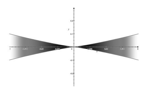
Figure 2. The growth condition required in (H2): the shaded area is the region $\{\lvert x_{n+1}\rvert\leq G(x^{\prime})\}$ ($\alpha=0.51$) in the cylinder $\mathrm{C}(T,0,r_{0})$ with $r_{0}=0.1$.

Some comments on the hypotheses (H0)-(H1)-(H2) are now in order.

Remark 3.4.

A fundamental observation stemming directly from the definitions is that, in general, a stationary varifold may have multiple different tangent cones at a given point. In particular, (H0) and (H1) alone do not imply that $\mathbf{var}(T,Q)$ is the only tangent cone to $V_{0}$ at $x_{0}$ (nor that all tangent cones to $V_{0}$ at $x_{0}$ are actually flat). As a matter of fact, the only conclusions that one may draw from (H0) and (H1) are that the density $\Theta_{V_{0}}(x_{0})$ is an integer $Q\geq 2$ and that if $\mathbf{C}$ is tangent to $V_{0}$ at $x_{0}$ and $\mathrm{spt}(\|\mathbf{C}\|)$ is contained in an $n$-plane $T^{\prime}$ then $\mathbf{C}=\mathbf{var}(T^{\prime},Q)$ (as a consequence of the constancy lemma for stationary varifolds). The hypothesis (H2) resolves the ambiguity, so that in our setting $\mathbf{var}(T,Q)$ is the unique tangent cone to $V_{0}$ at $x_{0}$.

The following is the main result of this paper.

Theorem 3.5.

If Assumption 3.3 holds, then there exists a Brakke flow $\{V_{t}\}_{t\geq 0}$ with fixed boundary $\partial\Gamma_{0}$ such that:

• $\lim_{t\to 0^{+}}\|V_{t}\|=\|V_{0}\|=\mathcal{H}^{n}\mathbin{\vrule height=6.88889pt,depth=0.0pt,width=0.55974pt\vrule height=0.55974pt,depth=0.0pt,width=5.59721pt}_{\Gamma_{0}}$;

• $\|V_{t}\|(U)<\|V_{0}\|(U)$ for all $t>0$.

We observe explicitly that if $V_{0}$ is stationary then the constant flow $V_{t}=V_{0}$ for all $t\geq 0$ is an $n$-dimensional Brakke flow with fixed boundary $\partial\Gamma_{0}$: the only condition to verify is the validity of Brakke’s inequality (2.15), which can be readily deduced by

$$\|V_{t}\|(\phi(\cdot,t))\Big{|}_{t=t_{1}}^{t_{2}} = \|V_{0}\|(\phi(\cdot,t_{2})-\phi(\cdot,t_{1}))$$

$$= \|V_{0}\|\left(\int_{t_{1}}^{t_{2}}\frac{\partial\phi}{\partial t}(\cdot,t)\,dt\right)$$

$$\leq \int_{t_{1}}^{t_{2}}\|V_{0}\|(\frac{\partial\phi}{\partial t}(\cdot,t))\,dt\,.$$

Hence, for an initial datum as in Assumption 3.3, Theorem 3.5 is a statement of non-uniqueness of Brakke flow.

Remark 3.6.

In the light of the above discussion, one may consider the subset of $\mathbf{IV}_{n}(U)$ consisting of those stationary varifolds $V_{0}$ such that the assignment $V_{t}=V_{0}$ for all $t\geq 0$ defines the only Brakke flow starting with $V_{0}$. We will say that such a stationary varifold is dynamically stable. A natural question is whether dynamically stable stationary varifolds enjoy better regularity properties than what stationarity alone is able to guarantee. By Theorem 3.5, if $V_{0}=\mathbf{var}(\Gamma_{0},1)$ with $\Gamma_{0}$ as in Assumption 3.1 and if $V_{0}$ is dynamically stable then the set of points satisfying (H1) and (H2) is empty. As anticipated in the introduction, it is an open question whether this implies that the set of points satisfying (H1) alone is empty, too (in other words, whether (H0) and (H1) imply (H2)), although that appears to be the case in all known examples. Notice that if $V_{0}$ is such that the set of points as in (H1) is empty then, as a consequence of the celebrated regularity theorem by Allard [2] and of the recent results by Naber and Valtorta [14], $\Gamma_{0}$ is an embedded real analytic $n$-dimensional minimal hypersurface in $U$ outside of a countably $(n-1)$-rectifiable singular set $\mathcal{S}$ (hence, in particular, such that $\mathcal{H}^{n-1+\delta}(\mathcal{S})=0$ for every $\delta>0$).

The rest of the paper is devoted to the proof of Theorem 3.5. The proof is constructive, and it roughly proceeds as follows. First, we modify the set $\Gamma_{0}$ in a small ball of radius $\varepsilon$ centered at $x_{0}=0$, so to have a quantifiable drop of its mass: we shall call this modification a “hole nucleation” in $\Gamma_{0}$. Then, we use our existence theorem from [19] to produce a Brakke flow (with fixed boundary $\partial\Gamma_{0}$) starting with this modified set $\Gamma_{0}^{\varepsilon}$. Using an iterative procedure which hinges upon Brakke’s “expanding hole lemma” [6, Lemma 6.5] (of which we present a detailed proof for the reader’s convenience), we show that this hole “expands” at future times: in particular, a hole of size $\sim\varepsilon$ at time $t=0$ becomes almost a hole of size $\sim 2^{j}\,\varepsilon$ at time $t\sim 2^{2j}\,\varepsilon^{2}$. The “almost” above accounts for an error occurring at each iteration which needs to be estimated in order to make sure that the evolving varifolds never re-gain the initial mass drop. The growth assumption (H2) is crucial to perform this estimate. The final product of this iterative process is a Brakke flow (depending on the size $\varepsilon$ of the initial hole nucleation) which, at a time $\bar{t}>0$, has strictly less mass than $\Gamma_{0}$, with both $\bar{t}$ and the mass loss independent of $\varepsilon$: the Brakke flow in the statement is then obtained in the limit as $\varepsilon\to 0^{+}$.

4. Hole nucleation

In this section we show that, given $U$, $\Gamma_{0}$, and $\{E_{0,i}\}_{i=1}^{N}$ as in Assumption 3.3, there exist Brakke flows starting from a set $\Gamma_{0}^{\varepsilon}$ obtained by modifying $\Gamma_{0}$ in a small ball $U_{2\varepsilon}$ around $x_{0}=0$ in a way to obtain a quantifiable drop of its mass, and we discuss the limits of such Brakke flows as $\varepsilon\to 0^{+}$. Informally, we may say that $\Gamma_{0}^{\varepsilon}$ is obtained by “making a hole” of radius $\sim\varepsilon$ in $\Gamma_{0}$. The details of the construction of $\Gamma_{0}^{\varepsilon}$ are contained in the following lemma.

Lemma 4.1.

Let $U$, $\Gamma_{0}$, $\{E_{0,i}\}_{i=1}^{N}$, and $T$ be as in Assumption 3.3. There exists $\varepsilon_{0}>0$ such that, for all $\varepsilon\in(0,\varepsilon_{0}]$, there exist a relatively closed and $\mathcal{H}^{n}$-rectifiable set $\Gamma_{0}^{\varepsilon}\subset U$, a family $\{E_{0,i}^{\varepsilon}\}_{i=1}^{N}$ of pairwise disjoint non-empty open subsets of $U$ with finite perimeter such that:

• $\Gamma_{0}^{\varepsilon}\setminus U_{2\varepsilon}=\Gamma_{0}\setminus U_{2\varepsilon}$ and $E_{0,i}^{\varepsilon}\setminus U_{2\varepsilon}=E_{0,i}\setminus U_{2\varepsilon}$ for each $i=1,\ldots,N$;

• $\Gamma_{0}^{\varepsilon}=U\setminus\cup_{i=1}^{N}E_{0,i}^{\varepsilon}$;

• $\Gamma_{0}^{\varepsilon}\cap U_{2\varepsilon}\subset\{(x^{\prime},x_{n+1}):|x_{n+1}|\leq G(x^{\prime})\}$;

• $\mathcal{H}^{n}(\Gamma_{0}^{\varepsilon}\cap U_{2\varepsilon})\leq(4\varepsilon)^{n}\omega_{n}(Q+1)$;

• $\mathcal{H}^{n}(\mathrm{C}(T,0,\varepsilon)\cap U_{2\varepsilon}\cap\Gamma_{0}^{\varepsilon})\leq\omega_{n}\varepsilon^{n}$.

Proof.

As usual, we assume without loss of generality that $T=\mathbb{R}^{n}\times\{0\}$, and thus we write $x=(x^{\prime},x_{n+1})\in\mathbb{R}^{n+1}=T\oplus T^{\perp}$. Furthermore, we let $V_{0}=\mathbf{var}(\Gamma_{0},1)$, so that, setting $\eta_{r}(x)=x/r$, we have $\lim_{r\rightarrow 0+}(\eta_{r})_{\sharp}V_{0}={\bf var}(T,Q)$ as varifolds. Define $\Gamma^{\varepsilon}:=\eta_{\varepsilon}(\Gamma_{0})$, $V^{\varepsilon}:=(\eta_{\varepsilon})_{\sharp}V_{0}$ and $E^{\varepsilon}_{i}:=\eta_{\varepsilon}(E_{0,i})$ for each $i=1,\ldots,N$ for simplicity. By (H2), there exists a sufficiently small $\varepsilon_{0}>0$ such that for all $\varepsilon\in(0,\varepsilon_{0}]$, we have

$$U_{2}\cap\Gamma^{\varepsilon}\subset\{|x_{n+1}|\leq 1/20\}.$$ (4.1)

We may additionally assume that $E_{i}^{\varepsilon}\setminus U_{2}\neq\emptyset$ for all $i$. In the following, let $\delta=1/5$ and define the following function $\mathrm{g}\colon\mathbb{R}^{n+1}\to\mathbb{R}^{n+1}$ as in [12, Proof of Lemma 4.7]. For $\lvert x^{\prime}\rvert\leq 1$, we set

$${\rm g}(x^{\prime},x_{n+1})=\begin{cases}(x^{\prime},x_{n+1})&\mbox{if $\lvert x_{n+1}\rvert\geq\delta$}\,,\\ (x^{\prime},0)&\mbox{if $\lvert x_{n+1}\rvert\leq\frac{\delta}{2}$}\,,\\ (x^{\prime},2\,x_{n+1}-\delta)&\mbox{if $\frac{\delta}{2}\leq x_{n+1}\leq\delta$}\,,\\ (x^{\prime},2\,x_{n+1}+\delta)&\mbox{if $-\delta\leq x_{n+1}\leq-\frac{\delta}{2}$}\,,\end{cases}$$ (4.2)

whereas in the region $1\leq\lvert x^{\prime}\rvert\leq 1+\delta$ we set

$${\rm g}(x^{\prime},x_{n+1})=\begin{cases}(x^{\prime},x_{n+1})&\mbox{if $\lvert x_{n+1}\rvert\geq\delta$ or $\lvert x_{n+1}\rvert\leq\lvert x^{\prime}\rvert-1$}\,,\\ (x^{\prime},\lvert x^{\prime}\rvert-1)&\mbox{if $\lvert x^{\prime}\rvert-1\leq x_{n+1}\leq\frac{\lvert x^{\prime}\rvert-1}{2}+\frac{\delta}{2}$}\,,\\ (x^{\prime},2\,x_{n+1}-\delta)&\mbox{if $\frac{\lvert x^{\prime}\rvert-1}{2}+\frac{\delta}{2}\leq x_{n+1}\leq\delta$}\,,\\ (x^{\prime},1-\lvert x^{\prime}\rvert)&\mbox{if $\frac{1-\lvert x^{\prime}\rvert}{2}-\frac{\delta}{2}\leq x_{n+1}\leq 1-\lvert x^{\prime}\rvert$}\,,\\ (x^{\prime},2\,x_{n+1}+\delta)&\mbox{if $-\delta\leq x_{n+1}\leq\frac{1-\lvert x^{\prime}\rvert}{2}-\frac{\delta}{2}$}\,.\end{cases}$$ (4.3)

Finally, we set

$${\rm g}(x^{\prime},x_{n+1})=(x^{\prime},x_{n+1})\qquad\mbox{if $\lvert x^{\prime}\rvert>1+\delta$}\,;$$ (4.4)

see Figure 3.

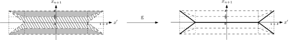
Figure 3. The map ${\rm g}$.

One may check that ${\rm g}$ is a Lipschitz map with ${\rm Lip}({\rm g})\leq 2$. Next, define

$$\tilde{E}_{i}^{\varepsilon}:={\rm int}({\rm g}(E_{i}^{\varepsilon}))\quad\mbox{ and }\quad E_{0,i}^{\varepsilon}:=\eta_{1/\varepsilon}(\tilde{E}_{i}^{\varepsilon})$$ (4.5)

for each $i=1,\ldots,N$, as well as

$$\tilde{\Gamma}^{\varepsilon}:=\eta_{\varepsilon}(U)\setminus\cup_{i=1}^{N}\tilde{E}_{i}^{\varepsilon}\quad\mbox{ and }\quad\Gamma_{0}^{\varepsilon}:=\eta_{1/\varepsilon}(\tilde{\Gamma}^{\varepsilon})\,.$$ (4.6)

Since ${\rm g}$ is a retraction map, one can check that $\tilde{E}_{1}^{\varepsilon},\ldots,\tilde{E}_{N}^{\varepsilon}$ are mutually disjoint open sets, and so are $E_{0,1}^{\varepsilon},\ldots,E_{0,N}^{\varepsilon}$. It follows from the definition of ${\rm g}$ that $E_{i}^{\varepsilon}\setminus U_{2}=\tilde{E}_{i}^{\varepsilon}\setminus U_{2}$ for $i=1,\ldots,N$. Thus (1) is satisfied for $\Gamma_{0}^{\varepsilon}$ and $E_{0,i}^{\varepsilon}$, and (2) holds by construction. We next check

$$\tilde{\Gamma}^{\varepsilon}\subset{\rm g}(\Gamma^{\varepsilon}).$$ (4.7)

We only need to prove the inclusion on the set on which the map ${\rm g}$ is not one-to-one, namely on $\{(x^{\prime},1-|x^{\prime}|),(x^{\prime},|x^{\prime}|-1):1\leq|x^{\prime}|<1+\delta\}\cup(T\cap U_{1})$. Note that any point $x$ of this set has the property that ${\rm g}^{-1}(x)$ is a closed line segment, say $I$, perpendicular to $T$. If $x\notin{\rm g}(\Gamma^{\varepsilon})$, that is, $I\cap\Gamma^{\varepsilon}=I\cap\cup_{i=1}^{N}\partial E_{i}^{\varepsilon}=\emptyset$, then there must exist some $E_{i}^{\varepsilon}$ such that $I\subset E_{i}^{\varepsilon}$. Then one can see that $x$ is an interior point of ${\rm g}(E_{i}^{\varepsilon})$, so that $x\in\tilde{E}_{i}^{\varepsilon}$ and not in $\tilde{\Gamma}^{\varepsilon}$. This proves (4.7). The inclusion (4.7) moreover proves that $\tilde{\Gamma}^{\varepsilon}$ is countably $n$-rectifiable. From the definition of ${\rm g}$, we have $|T^{\perp}({\rm g}(x))|\leq|T^{\perp}(x)|$, and (3) follows from this fact. Since ${\rm Lip}({\rm g})\leq 2$ and $\mathcal{H}^{n}(U_{2}\cap\Gamma^{\varepsilon})\leq 2^{n}\omega_{n}(Q+1)$ for all small $\varepsilon$, the area formula guarantees that $\mathcal{H}^{n}(U_{2}\cap\tilde{\Gamma}^{\varepsilon})\leq 4^{n}\omega_{n}(Q+1)$. This gives (4) after change of variables. In particular, $\tilde{\Gamma}^{\varepsilon}$ has no interior points and finite $\mathcal{H}^{n}$ measure, it holds $\tilde{\Gamma}^{\varepsilon}=\cup_{i=1}^{N}\partial\tilde{E}_{i}^{\varepsilon}$, and the sets $E_{0,1}^{\varepsilon},\ldots,E_{0,N}^{\varepsilon}$ have bounded perimeter. Finally, from the definition of ${\rm g}$, we have (writing $\mathrm{C}(r)$ for $\mathrm{C}(T,0,r)$)

$$\begin{split}&{\rm g}(\mathrm{C}(1)\cap\{\delta/2\leq x_{n+1}\leq\delta\})=\mathrm{C}(1)\cap\{0\leq x_{n+1}\leq\delta\},\\ &{\rm g}(\mathrm{C}(1)\cap\{-\delta\leq x_{n+1}\leq-\delta/2\})=\mathrm{C}(1)\cap\{-\delta\leq x_{n+1}\leq 0\}\,.\end{split}$$ (4.8)

Since $\cup_{i=1}^{N}\partial E_{i}^{\varepsilon}=\Gamma^{\varepsilon}$ in $U_{2}$ and $E_{1}^{\varepsilon},\ldots,E_{N}^{\varepsilon}$ are mutually disjoint, (4.1) shows that there exist $i_{1},i_{2}\in\{1,\ldots,N\}$ such that

$$(U_{2}\cap\{x_{n+1}\geq\delta/2\})\subset E_{i_{1}}^{\varepsilon}\,\,\mbox{ and }\,\,(U_{2}\cap\{x_{n+1}\leq-\delta/2\})\subset E_{i_{2}}^{\varepsilon}.$$ (4.9)

We claim that

$$\mathrm{C}(1)\cap U_{2}\cap\tilde{\Gamma}^{\varepsilon}\subset T\cap B_{1}.$$ (4.10)

Note that (4.8) and (4.9) imply that $\mathrm{C}(1)\cap\{0<x_{n+1}\leq\delta\}\subset\tilde{E}_{i_{1}}^{\varepsilon}$ and $\mathrm{C}(1)\cap\{-\delta\leq x_{n+1}<0\}\subset\tilde{E}_{i_{2}}^{\varepsilon}$. Thus, we have $\tilde{\Gamma}^{\varepsilon}\cap\mathrm{C}(1)\cap\{-\delta\leq x_{n+1}\leq\delta\}\subset T\cap B_{1}$. Since $U_{2}\cap\Gamma^{\varepsilon}\cap\{|x_{n+1}|\geq\delta\}=\emptyset$, this proves (4.10), and consequently we have (5). ∎

By [19, Theorems 2.2 & 2.3] we have then immediately the following existence of Brakke flows starting with $\Gamma_{0}^{\varepsilon}$.

Proposition 4.2.

With $\Gamma_{0}^{\varepsilon}$ and $\{E_{0,i}^{\varepsilon}\}_{i=1}^{N}$ given in Lemma 4.1, there exists a Brakke flow $\{V_{t}^{\varepsilon}\}_{t\geq 0}$ with fixed boundary $\partial\Gamma_{0}$ and $\|V_{0}^{\varepsilon}\|=\mathcal{H}^{n}\mathbin{\vrule height=6.88889pt,depth=0.0pt,width=0.55974pt\vrule height=0.55974pt,depth=0.0pt,width=5.59721pt}_{\Gamma_{0}^{\varepsilon}}$. For each $i=1,\ldots,N$, there exists a one-parameter family $\{E_{i}^{\varepsilon}(t)\}_{t\geq 0}$ of open sets $E_{i}^{\varepsilon}(t)\subset U$ with the properties described in [19, Theorem 2.3].

Proof.

To apply [19, Theorem 2.2 & 2.3] we only need to check that (A1)-(A4) in Assumption 3.1 are satisfied with $U$, $\Gamma_{0}^{\varepsilon}$, and $\{E_{0,i}^{\varepsilon}\}_{i=1}^{N}$ for each $\varepsilon\in(0,\varepsilon_{0}]$. These follow from Lemma 4.1 (1),(2). ∎

Proposition 4.3.

For any sequence $\{\varepsilon_{j}\}_{j=1}^{\infty}\subset(0,\varepsilon_{0}]$ converging to $0$, there exist a subsequence (denoted by the same index) and a Brakke flow $\{V_{t}\}_{t\geq 0}$ with fixed boundary $\partial\Gamma_{0}$ such that $\lim_{j\rightarrow\infty}\|V_{t}^{\varepsilon_{j}}\|=\|V_{t}\|$ in $U$ for each $t\geq 0$ and $\lim_{t\rightarrow 0+}\|V_{t}\|=\|V_{0}\|=\mathcal{H}^{n}\mathbin{\vrule height=6.88889pt,depth=0.0pt,width=0.55974pt\vrule height=0.55974pt,depth=0.0pt,width=5.59721pt}_{\Gamma_{0}}$.

Proof.

Since $\|V_{t}^{\varepsilon}\|(U)\leq\|V_{0}^{\varepsilon}\|(U)=\mathcal{H}^{n}(\Gamma_{0}^{\varepsilon})=\mathcal{H}^{n}(\Gamma_{0})+o(1)$ as $\varepsilon\rightarrow 0^{+}$ for all $t>0$, we have a uniform mass bound for the family. Such a family of Brakke flows is known to be compact (see [9] and [20, Section 3.2]), thus there exists a subsequence (denoted by the same index) and a limit Brakke flow $\{V_{t}\}_{t\geq 0}$ such that $\lim_{j\rightarrow\infty}\|V_{t}^{\varepsilon_{j}}\|=\|V_{t}\|$ as Radon measures on $U$ for all $t\geq 0$. By Lemma 4.1(4), we also have $\|V_{0}\|=\mathcal{H}^{n}\mathbin{\vrule height=6.88889pt,depth=0.0pt,width=0.55974pt\vrule height=0.55974pt,depth=0.0pt,width=5.59721pt}_{\Gamma_{0}}$. For each $B_{r}(x)\times[t_{1},t_{2}]\subset\joinrel\subset U\times(0,\infty)$ and $i\in\{1,\ldots,N\}$, the argument for the proof of [11, Theorem 3.5(6)] (which is equally valid for the fixed boundary case away from $\partial U$) shows that $\mathcal{L}^{n+1}(E_{i}^{\varepsilon}(t)\cap B_{r}(x))$ is $\frac{1}{2}$-Hölder continuous as a function of $t\in[t_{1},t_{2}]$, with uniformly bounded Hölder norm independently of $\varepsilon$. Also, if $0\notin B_{r+2\varepsilon}(x)$, the same proof shows that $\mathcal{L}^{n+1}(B_{r}(x)\cap E_{i}^{\varepsilon}(t))$ is continuous at $t=0$ with uniform modulus of continuity with respect to $\varepsilon$. Since $\|\partial^{*}E_{i}^{\varepsilon}(t)\|\leq\|V_{t}^{\varepsilon}\|$ for all $t\geq 0$ (see [19, Theorem 2.3(8)]), and since the latter is uniformly bounded, by a suitable diagonal argument and the uniform continuity in $t$, one can prove that there exists a further subsequence (denoted by the same index) and a family of sets of finite perimeter $\{\tilde{E}_{i}(t)\}_{t\geq 0}$ in $U$ for $i=1,\ldots,N$ such that $\lim_{j\rightarrow\infty}\mathcal{L}^{n+1}(E_{i}^{\varepsilon_{j}}(t)\,\triangle\,\tilde{E}_{i}(t))=0$ for all $t\geq 0$ and $\mathcal{L}^{n+1}(B_{r}(x)\cap\tilde{E}_{i}(t))$ is $C^{1/2}((0,\infty))\cap C([0,\infty))$ as a function of $t$ for any $B_{r}(x)\subset\joinrel\subset U$. For each $t\geq 0$, $\{\tilde{E}_{i}(t)\}_{i=1}^{N}$ satisfies $\mathcal{L}^{n+1}(\tilde{E}_{i}(t)\cap\tilde{E}_{i^{\prime}}(t))=0$ for $i\neq i^{\prime}$ and $\mathcal{L}^{n+1}(U\setminus\cup_{i=1}^{N}\tilde{E}_{i}(t))=0$. By Lemma 4.1(1), we also have $\tilde{E}_{i}(0)=E_{0,i}$ for each $i=1,\ldots,N$.

Define the space-time Radon measure $d\mu:=d\|V_{t}\|dt$ on $U\times(0,\infty)$ and $({\rm spt}\,\mu)_{t}:=\{x\in U:(x,t)\in{\rm spt}\,\mu\}$ for each $t>0$. By the fact that $\{V_{t}\}_{t\geq 0}$ is a Brakke flow, we have for all $t>0$

$${\rm spt}\,\|V_{t}\|\subset({\rm spt}\,\mu)_{t} \mathcal{H}^{n}(({\rm spt}\,\mu)_{t}\cap\tilde{U})<\infty \tilde{U}\subset\joinrel\subset U$$ and for all (4.11)

by [11, Lemma 10.1] and [11, Corollary 10.8], respectively. Since

$$\|\partial^{*}\tilde{E}_{i}(t)\|\leq\liminf_{j\rightarrow\infty}\|\partial^{*}E_{i}^{\varepsilon_{j}}(t)\|\leq\lim_{j\rightarrow\infty}\|V_{t}^{\varepsilon_{j}}\|=\|V_{t}\|$$ (4.12)

for all $t\geq 0$, (4.11) shows that ${\rm spt}\,\|\partial^{*}\tilde{E}_{i}(t)\|\subset({\rm spt}\,\mu)_{t}$ for all $t>0$. In particular, on each connected component of $U\setminus({\rm spt}\,\mu)_{t}$, $\chi_{\tilde{E}_{i}(t)}$ is constant. Then, it follows using the continuity property of $\mathcal{L}^{n+1}(B_{r}(x)\cap\tilde{E}_{i}(t))$ that the open set $(U\times(0,\infty))\setminus{\rm spt}\,\mu$ can be decomposed into mutually disjoint open sets $E_{1},\ldots,E_{N}$ such that $\cup_{i=1}^{N}E_{i}=(U\times(0,\infty))\setminus{\rm spt}\,\mu$ and such that $\mathcal{L}^{n+1}(\tilde{E}_{i}(t)\,\triangle\,\{x\in U:(x,t)\in E_{i}\})=0$ for all $t>0$. We may redefine $E_{i}(t)=\{x\in U:(x,t)\in E_{i}\}$, which is open and $\mathcal{L}^{n+1}(\tilde{E}_{i}(t)\,\triangle\,E_{i}(t))=0$. By definition, we have $U\setminus\cup_{i=1}^{N}E_{i}(t)=({\rm spt}\,\mu)_{t}$ and (4.11) shows that $U\setminus\cup_{i=1}^{N}E_{i}(t)$ has no interior points, so that we have $\cup_{i=1}^{N}\partial E_{i}(t)=({\rm spt}\,\mu)_{t}$ for all $t>0$. The continuity at $t=0$ shows that $\lim_{t\rightarrow 0+}\mathcal{L}^{n+1}(E_{i}(t)\,\triangle\,E_{0,i})=0$ for $i=1,\ldots,N$.

By [19, Theorem 2.3(5)(11)], for each $j$ and all $t\geq 0$, ${\rm spt}\,\|V_{t}^{\varepsilon_{j}}\|\subset{\rm conv}(\Gamma_{0}^{\varepsilon_{j}}\cup\partial\Gamma_{0})$. Since the difference of $\Gamma_{0}^{\varepsilon_{j}}$ and $\Gamma_{0}$ lies within $U_{2\varepsilon_{j}}$, we may conclude that ${\rm spt}\|V_{t}\|\subset{\rm conv}(\Gamma_{0}\cup\partial\Gamma_{0})$ for all $t\geq 0$, and one may deduce that $({\rm spt}\,\mu)_{t}\subset{\rm conv}(\Gamma_{0}\cup\partial\Gamma_{0})$ for $t>0$. We also can see from the last claim that

$$E_{i}(t)\setminus{\rm conv}(\Gamma_{0}\cup\partial\Gamma_{0})=E_{0,i}\setminus{\rm conv}(\Gamma_{0}\cup\partial\Gamma_{0})$$ (4.13)

for all $t\geq 0$ and $i=1,\ldots,N$.

Next, we prove that $V_{t}$ has a fixed boundary $\partial\Gamma_{0}$, i.e., $({\rm clos}\,({\rm spt}\|V_{t}\|))\setminus U=\partial\Gamma_{0}$. The inclusion $\subset$ follows from ${\rm spt}\|V_{t}\|\subset{\rm conv}(\Gamma_{0}\cup\partial\Gamma_{0})$, the definition of $\partial\Gamma_{0}$ and the strict convexity of $U$. For the converse inclusion, assume that we have $x\in\partial\Gamma_{0}$ and there exists $r>0$ such that ${\rm spt}\,\|V_{t}\|\cap U_{r}(x)=\emptyset$. Then we have $\|V_{t}\|(U_{r}(x))=0$. But then (4.12) shows $\|\partial^{*}E_{i}(t)\|(U_{r}(x)\cap U)=0$ for $i=1,\ldots,N$. On the other hand, by (4.13) and (A4) of Assumption 3.1, we must have some $i_{1}\neq i_{2}$ such that $U_{r}(x)\cap E_{i_{k}}(t)\neq\emptyset$ for $k=1,2$. These are not compatible. Thus we have $({\rm clos}\,({\rm spt}\|V_{t}\|))\setminus U=\partial\Gamma_{0}$.

Finally, $\lim_{t\rightarrow 0+}\|V_{t}\|=\mathcal{H}^{n}\mathbin{\vrule height=6.88889pt,depth=0.0pt,width=0.55974pt\vrule height=0.55974pt,depth=0.0pt,width=5.59721pt}_{\Gamma_{0}}$ follows from the argument in [19, Proposition 6.10] under the condition (A5) of Assumption 3.1 that $\mathcal{H}^{n}(\Gamma_{0}\setminus\cup_{i=1}^{N}\partial^{*}E_{0,i})=0$. Indeed, for any $\phi\in C_{c}(U;\mathbb{R}^{+})$,

$$\limsup_{t\rightarrow 0+}\|V_{t}\|(\phi)\leq\|V_{0}\|(\phi)=\mathcal{H}^{n}\mathbin{\vrule height=6.88889pt,depth=0.0pt,width=0.55974pt\vrule height=0.55974pt,depth=0.0pt,width=5.59721pt}_{\Gamma_{0}}(\phi)$$

follows from the property of Brakke flow, and

$$\begin{split}&2\mathcal{H}^{n}\mathbin{\vrule height=6.88889pt,depth=0.0pt,width=0.55974pt\vrule height=0.55974pt,depth=0.0pt,width=5.59721pt}_{(\cup_{i=1}^{N}\partial^{*}E_{0,i})}(\phi)=\sum_{i=1}^{N}\|\nabla\chi_{E_{0,i}}\|(\phi)\leq\sum_{i=1}^{N}\liminf_{t\rightarrow 0+}\|\nabla\chi_{E_{i}(t)}\|(\phi)\\ &\leq\liminf_{t\rightarrow 0+}\sum_{i=1}^{N}\|\nabla\chi_{E_{i}(t)}\|(\phi)\leq 2\liminf_{t\rightarrow 0+}\|V_{t}\|(\phi).\end{split}$$ (4.14)

These show that $\lim_{t\rightarrow 0+}\|V_{t}\|(\phi)=\mathcal{H}^{n}\mathbin{\vrule height=6.88889pt,depth=0.0pt,width=0.55974pt\vrule height=0.55974pt,depth=0.0pt,width=5.59721pt}_{\Gamma_{0}}(\phi)$ if $\mathcal{H}^{n}(\Gamma_{0}\setminus\cup_{i=1}^{N}\partial^{*}E_{0,i})=0$. ∎

5. Brakke’s expanding holes lemma

In this section, we discuss Brakke’s expanding holes lemma [6, Lemma 6.5], which is a key tool towards the proof of Theorem 3.5. Given its importance in the following arguments, and for the reader’s convenience, we provide a detailed proof. The lemma is valid for Brakke flow of any codimension, and we will state it and prove it in such generality. Hence, in this section $k$ will be a fixed integer in $\{1,\ldots,n\}$, and $T$ will be a plane in $\mathbf{G}(n+1,k)$. Before stating the lemma, we will need some preliminary notation.

Definition 5.1.

Let $\chi\colon\mathbb{R}^{k}\to\mathbb{R}^{+}$ be a smooth cut-off function $0\leq\chi\leq 1$, such that:

• $\chi(x)$ is a decreasing function of the radial variable $r=\lvert x\rvert\,;$

• $\mathrm{spt}(\chi)\subset U^{k}_{1}(0)\,;$

• $\chi(x)=1$ if $0\leq\lvert x\rvert<1-\zeta$ for a small positive number $\zeta$ .

We will denote

$$\rho:=\sup_{x\in\mathbb{R}^{k}}\left\{\lvert\nabla\chi(x)\rvert+2\|D^{2}\chi(x)\|\right\}\,,$$ (5.1)

and we shall often use the fact that $\lvert\nabla\chi(x)\rvert^{2}/\chi(x)\leq 2\sup\|D^{2}\chi\|\leq\rho$.

For a radius $R>0$, we set

$$\chi_{T,R}(x):=\chi(T(x)/R)\,.$$ (5.2)

Since the plane $T$ will always be kept fixed, we will drop the subscript _T in (5.2) and denote the cylindrical cut-off at scale $R$ simply by $\chi_{R}$. Along the same lines, we also recall that $\mathrm{C}(R)$ denotes the infinite cylinder orthogonal to $T$ centered at the origin and with radius $R$.

Finally, let us collect the following well-known facts concerning the orthogonal projection operators onto planes in $\mathbf{G}(n+1,k)$. The reader can consult [10, Lemma 11.1] for their proofs.

Lemma 5.2.

For $S,T\in\mathbf{G}(n+1,k)$ and $v\in\mathbb{R}^{n+1}$, the following holds.

$${\rm I}\cdot T =k\,,\quad T^{t}=T\,,\quad T\circ T=T\,,\quad T\circ T^{\perp}=0\,.$$ (5.3)

$$0 \leq k-S\cdot T=S^{\perp}\cdot T\leq k\,\|S-T\|^{2}\,.$$ (5.4)

$$0 \leq\|S-T\|^{2}\leq(S-T)\cdot(S-T)=2\,T^{\perp}\cdot S\,.$$ (5.5)

$$\lvert T(S^{\perp}(v))\rvert \leq\|T-S\|\,\lvert v\rvert\,.$$ (5.6)

$$\lvert T(S^{\perp}(T(v)))\rvert \leq\|T-S\|^{2}\,\lvert v\rvert\,.$$ (5.7)

Lemma 5.3 (Brakke’s expanding holes lemma).

Let $T\in\mathbf{G}(n+1,k)$, $0\leq t_{1}<t_{2}<\infty$, $0<R_{1}<R_{2}$, $0<\hat{R}_{1}<\hat{R}_{2}$ and set

$$\sigma:=\frac{R_{2}^{2}-R_{1}^{2}}{t_{2}-t_{1}}\,,\qquad R(t)^{2}:=R_{1}^{2}+\sigma\,(t-t_{1})\,,\qquad\phi_{t}(x):=\chi_{R(t)}(x)=\chi(T(x)/R(t))\,.$$

Let $\{V_{t}\}_{t\in[t_{1},t_{2}]}$ be a $k$-dimensional Brakke flow in $C(R_{2})\cap\{|T^{\perp}(x)|<\hat{R}_{2}\}$ such that

$${\rm spt}\,\|V_{t}\|\cap\{\hat{R}_{1}<|T^{\perp}(x)|<\hat{R}_{2}\}=\emptyset\qquad\mbox{for all $t\in[t_{1},t_{2}]$}.$$ (5.8)

For a.e. $t\in\left[t_{1},t_{2}\right]$, define the functions $\alpha(t)$ and $\mu(t)$ by

$$\mu(t)^{2} :=\int_{\mathrm{C}(R(t))}\lvert T^{\perp}(x)\rvert^{2}\,d\|V_{t}\|(x)\,,$$ (5.9)

$$\alpha(t)^{2} :=\int\lvert h(x,V_{t})\rvert^{2}\,\phi_{t}^{2}(x)\,d\|V_{t}\|(x)\,.$$ (5.10)

Then, we have for a.e. $t\in[t_{1},t_{2}]$

$$\delta(V_{t},\phi_{t}^{2})(h(\cdot,V_{t}))<-\frac{\alpha(t)^{2}}{2}+320\,\rho^{2}R(t)^{-4}\mu(t)^{2}\,.$$ (5.11)

Furthermore, there is $M=M(k,\sigma,\rho)<\infty$ such that if $\mu\in\left[0,\infty\right)$ satisfies

$$\mu(t)^{2}\leq\mu^{2}\,R(t)^{k+2}\qquad\mbox{for a.e.\leavevmode\nobreak\ $t\in\left[t_{1},t_{2}\right]$}\,,$$ (5.12)

then

$$R_{2}^{-k}\|V_{t_{2}}\|(\phi_{t_{2}}^{2})\leq R_{1}^{-k}\|V_{t_{1}}\|(\phi_{t_{1}}^{2})+M\mu^{2}\log(R_{2}/R_{1})\,.$$ (5.13)

Remark 5.4.

The main conclusion of the lemma, equation (5.13), establishes an upper bound on the gain of mass density ratio for Brakke flow at times $t_{1},t_{2}$ in enlarging cylinders $\mathrm{C}(R_{1})\subset\mathrm{C}(R_{2})$. The difference in mass density ratios is bounded above by the supremum, in the interval $[t_{1},t_{2}]$, of the (scale invariant) $L^{2}$-excess of $V_{t}$ with respect to the plane $T$, namely the function $R(t)^{-(k+2)}\mu(t)^{2}$.

Proof.

In the following, we use test functions $\phi_{t}^{2}$ in (2.15), which do not have compact support in $\mathrm{C}(R_{2})$. On the other hand, due to (5.8), we may multiply $\phi_{t}^{2}$ by a suitable cut-off function which is identically equal to $1$ on $\{|T^{\perp}(x)|\leq\hat{R}_{1}\}$ and which vanishes on $\{|T^{\perp}(x)|\geq\hat{R}_{2}\}$ and so that the resulting functions belong to $C_{c}(\mathrm{C}(R_{2}))$. The computation is not affected at all so that it is understood in the following that we implicitly modify $\phi_{t}^{2}$ as such without changing the notation. First, we show the validity of the dissipation inequality (5.11). Applying (2.11) with $\phi=\phi_{t}^{2}$, using that

$$\nabla[\phi_{t}^{2}]=2\phi_{t}\nabla\phi_{t}\,,\qquad\nabla\phi_{t}(x)=R(t)^{-1}T[\nabla\chi(T(x)/R(t))]\in T\,,$$ (5.14)

and exploiting Brakke’s perpendicularity Theorem 2.6 we calculate

$$\begin{split}\delta(V_{t},\phi_{t}^{2})(h(\cdot,V_{t}))&=-\int\lvert h(x,V_{t})\rvert^{2}\,\phi_{t}^{2}(x)\,d\|V_{t}\|(x)+2\int h(x,V_{t})\cdot S^{\perp}(\nabla\phi_{t}(x))\,\phi_{t}(x)\,dV_{t}(x,S)\\ &\leq-\alpha(t)^{2}+2\int\lvert h(x,V_{t})\rvert\,\|S-T\|\,\lvert\nabla\phi_{t}(x)\rvert\,\phi_{t}(x)\,dV_{t}(x,S)\\ &\leq-\frac{3}{4}\alpha(t)^{2}+4\int\|S-T\|^{2}\,\lvert\nabla\phi_{t}(x)\rvert^{2}\,dV_{t}(x,S)\,.\end{split}$$ (5.15)

In order to estimate the second term, we apply (a slight modification of) [10, Lemma 11.2] with $\phi$ replaced by $\lvert\nabla\phi_{t}\rvert$ to deduce

$$\begin{split}&\quad\int\|S-T\|^{2}\,\lvert\nabla\phi_{t}(x)\rvert^{2}\,dV_{t}(x,S)\\ &\leq 16\int\lvert T^{\perp}(x)\rvert^{2}\,\lvert\nabla\lvert\nabla\phi_{t}(x)\rvert\rvert^{2}\,d\|V_{t}\|(x)\\ &\hskip 56.9055pt+4\left\{\left(\int\lvert h(x,V_{t})\rvert^{2}\,\phi_{t}^{2}(x)\,d\|V_{t}\|(x)\right)\left(\int\lvert T^{\perp}(x)\rvert^{2}\,\lvert\nabla\phi_{t}(x)\rvert^{4}\,\phi_{t}^{-2}(x)\right)\right\}^{\nicefrac{{1}}{{2}}}\\ &\leq 16\rho^{2}R(t)^{-4}\mu(t)^{2}+4\rho R(t)^{-2}\alpha(t)\mu(t)\\ &\leq\frac{\alpha(t)^{2}}{16}+80\rho^{2}R(t)^{-4}\mu(t)^{2}\,.\end{split}$$ (5.16)

Equations (5.15) and (5.16) together prove (5.11).

In order to prove (5.13), we observe that, heuristically,

$$\partial_{t}\left[R(t)^{-k}\,\|V_{t}\|(\phi_{t}^{2})\right]=-kR^{\prime}(t)R(t)^{-k-1}\,\|V_{t}\|(\phi_{t}^{2})+R(t)^{-k}\partial_{t}\left[\|V_{t}\|(\phi_{t}^{2})\right]\,,$$

which can be expressed rigorously in terms of the inequality

$$\left.R(t)^{-k}\|V_{t}\|(\phi_{t}^{2})\right|_{t=t_{1}}^{t_{2}}\leq\int_{t_{1}}^{t_{2}}R(t)^{-k}D\left[\|V_{t}\|(\phi_{t}^{2})\right]-kR^{\prime}(t)R(t)^{-k-1}\,\|V_{t}\|(\phi_{t}^{2})\,dt\,,$$ (5.17)

where $D\left[\|V_{t}\|(\phi_{t}^{2})\right]$ is the distributional derivative of $t\in\left[t_{2},t_{2}\right]\mapsto\|V_{t}\|(\phi_{t}^{2})$. On the other hand, since $\{V_{t}\}_{t\geq 0}$ is a Brakke flow, Brakke’s inequality (2.15) implies that, in the sense of distributions,

$$D\left[\|V_{t}\|(\phi_{t}^{2})\right]\leq\delta(V_{t},\phi_{t}^{2})(h(\cdot,V_{t}))+\|V_{t}\|(\partial_{t}[\phi_{t}^{2}])\,.$$ (5.18)

Since (5.11) controls the first addendum, we only have to estimate the second one. We first compute explicitly the time derivative $\partial_{t}[\phi_{t}^{2}]$, namely

$$\partial_{t}[\phi_{t}^{2}] = 2\,\phi_{t}\,\partial_{t}\phi_{t}=-2\,\phi_{t}\,R(t)^{-2}R^{\prime}(t)\,T(x)\cdot\nabla\chi(T(x)/R(t))=$$

$$= -2\,\phi_{t}\,R(t)^{-2}R^{\prime}(t)\,x\cdot T\left[\nabla\chi(T(x)/R(t))\right]$$

$$= -2\,\phi_{t}\,R(t)^{-1}R^{\prime}(t)\,x\cdot\nabla\phi_{t}(x)\,,$$

where we have used that $T$ is an orthogonal projection operator and the expression for $\nabla\phi_{t}$ in (5.14). Hence, we have

$$\|V_{t}\|(\partial_{t}[\phi_{t}^{2}])=R(t)^{-1}R^{\prime}(t)\underbrace{\int\left\{-2\,\phi_{t}(x)\,x\cdot\nabla\phi_{t}(x)\right\}\,d\|V_{t}\|(x)}_{A}\,.$$ (5.19)

Now, observe that, by the definition of first variation and generalized mean curvature,

$$-\int\phi_{t}^{2}(x)\,T(x)\cdot h(x,V_{t})\,d\|V_{t}\|(x) = \delta V_{t}(\phi_{t}^{2}\,T(\cdot))$$

$$= \int\nabla[\phi_{t}^{2}\,T(x)]\cdot S\,dV_{t}(x,S)$$

$$= k\,\|V_{t}\|(\phi_{t}^{2})+\int 2\,\phi_{t}\left[T(x)\otimes\nabla\phi_{t}\right]\cdot S\,dV_{t}(x,S)$$

$$\qquad\qquad\qquad+\int\phi_{t}^{2}\,(T\cdot S-k)\,dV_{t}(x,S)\,,$$

and since $[u\otimes v]\cdot S=S(v)\cdot u=S(u)\cdot v$ for a symmetric $S$, we have that

$$\int\left\{-2\,\phi_{t}\,\nabla\phi_{t}\cdot S(T(x))\right\}\,dV_{t}(x,S)$$

$$\hskip 28.45274pt=k\,\|V_{t}\|(\phi_{t}^{2})+\underbrace{\int\phi_{t}^{2}(x)\,T(x)\cdot h(x,V_{t})\,d\|V_{t}\|(x)}_{I_{1}}+\underbrace{\int\phi_{t}^{2}\,(T\cdot S-k)\,dV_{t}(x,S)}_{I_{2}}\,.$$

On the other hand, it also holds

$$\int\left\{-2\,\phi_{t}\,\nabla\phi_{t}\cdot S(T(x))\right\}\,dV_{t}(x,S)=A-\underbrace{\int\left\{-2\,\phi_{t}(x)\,\nabla\phi_{t}(x)\cdot[x-S(T(x))]\right\}\,dV_{t}(x,S)}_{I_{3}}\,,$$

so that

$$A=k\,\|V_{t}\|(\phi_{t}^{2})+I_{1}+I_{2}+I_{3}\,,$$ (5.20)

and we can estimate the three pieces one at a time.

In order to estimate the term $I_{1}$, we use Brakke’s perpendicularity theorem to write

$$I_{1}=\int\phi_{t}^{2}(x)\,S^{\perp}(T(x))\cdot h(x,V_{t})\,dV_{t}(x,S)\,,$$

so that, using $\lvert T(x)\rvert\leq R(t)$ on $\mathrm{spt}(\phi_{t})$ together with $2\,R(t)R^{\prime}(t)=\sigma$, we get from (5.3) that

$$\begin{split}\lvert I_{1}\rvert&\leq\int\phi_{t}^{2}(x)\,\|S-T\|\,\lvert T(x)\rvert\,\lvert h(x,V_{t})\rvert\,dV_{t}(x,S)\ \\ &\leq\frac{R(t)}{R^{\prime}(t)}\,\frac{\alpha(t)^{2}}{4}+\frac{\sigma}{2}\int\phi^{2}_{t}(x)\,\|S-T\|^{2}\,dV_{t}(x,S)\,.\end{split}$$ (5.21)

Using (5.4), we have, instead:

$$\lvert I_{2}\rvert\leq k\int\phi^{2}_{t}(x)\,\|S-T\|^{2}\,dV_{t}(x,S)\,.$$ (5.22)

Because $\nabla\phi_{t}\in T$ and $T\circ T=T$, $\nabla\phi_{t}\cdot[x-S(T(x))]=\nabla\phi_{t}\cdot T(S^{\perp}(T(T(x))))$, and thus (5.7) and Young’s inequality give

$$\begin{split}\lvert I_{3}\rvert&\leq 2\int\phi_{t}(x)\,\lvert\nabla\phi_{t}(x)\rvert\,\|S-T\|^{2}\,\lvert T(x)\rvert\,dV_{t}(x,S)\\ &\leq\int\phi^{2}_{t}(x)\,\|S-T\|^{2}\,dV_{t}(x,S)+R(t)^{2}\int\lvert\nabla\phi_{t}(x)\rvert^{2}\,\|S-T\|^{2}\,dV_{t}(x,S)\,.\end{split}$$ (5.23)

In turn, by [10, Lemma 11.2] we can further estimate

$$\int\phi^{2}_{t}(x)\,\|S-T\|^{2}\,dV_{t}(x,S)\leq 4\alpha(t)\mu(t)+4\rho R(t)^{-2}\mu^{2}(t)\,,$$ (5.24)

so that plugging (5.16) and (5.24) into (5.21), (5.22), and (5.23) yields

$$\lvert I_{1}\rvert+\lvert I_{2}\rvert+\lvert I_{3}\rvert\leq\frac{R(t)}{R^{\prime}(t)}\,\frac{\alpha(t)^{2}}{4}+C\,(\alpha(t)\mu(t)+R(t)^{-2}\mu(t)^{2})\,,$$ (5.25)

where $C$ is a constant depending only on $k,\sigma$ and $\rho$.

In particular, from (5.20) and the definition of $A$ we conclude the following bound:

$$\begin{split}&\|V_{t}\|(\partial_{t}[\phi_{t}^{2}])-k\,R(t)^{-1}R^{\prime}(t)\,\|V_{t}\|(\phi_{t}^{2})\\ &\leq\frac{\alpha(t)^{2}}{4}+C\,R^{\prime}(t)R(t)^{-1}\,(\alpha(t)\mu(t)+R(t)^{-2}\mu(t)^{2})\\ &\leq\frac{\alpha(t)^{2}}{2}+C\,\lvert R^{\prime}(t)R(t)^{-1}\rvert^{2}\,\mu(t)^{2}+C\,R^{\prime}(t)R(t)^{-3}\,\mu(t)^{2}\\ &\leq\frac{\alpha(t)^{2}}{2}+CR(t)^{-4}\mu(t)^{2}\,.\end{split}$$ (5.26)

In the last line, we used the identity $\sigma=2\,R^{\prime}(t)R(t)$: the constants $C$ are different from line to line throughout the calculation, but they all depend only on $k,\sigma$ and $\rho$. Now, we first use (5.18), (5.11) and (5.26), and then we multiply by $R(t)^{-k}$ in order to gain, thanks to $\sigma=2\,R^{\prime}(t)R(t)$ and the definition of $\mu$ in (5.12), the estimate

$$\begin{split}R(t)^{-k}D\left[\|V_{t}\|(\phi_{t}^{2})\right]&-kR^{\prime}(t)R(t)^{-k-1}\,\|V_{t}\|(\phi_{t}^{2})\\ &\leq\lvert R^{\prime}(t)R(t)^{-1}\rvert\,M\,\mu^{2}\,,\end{split}$$ (5.27)

where $M$ is a constant depending only on $k,\sigma$ an $\rho$.

The conclusion (5.13) then follows plugging (5.27) into (5.17). ∎

6. $L^{2}$ excess estimates

This section contains the technical results which will be needed in the proof of Theorem 3.5 in order to estimate the $L^{2}$ excess terms in the iterative applications of (5.13), representing the possible gains of mass density ratio at each iteration. A careful estimate of these terms is crucial to show that the limiting Brakke flow is not trivial.

We begin with the following result, which is an adaptation of [10, Proposition 6.5]. It states that the (scale invariant) $L^{2}$ excess of varifolds evolving according to Brakke flow in a given ball can be estimated uniformly in time with the $L^{2}$ excess of the initial datum in a larger ball, with an error terms which decays to zero exponentially fast as the magnifying factor of the ball diverges to infinity, provided said varifolds have uniformly bounded mass density ratio in such larger ball.

Proposition 6.1.

Let $R>0$, $2\leq L<\infty$, and let $\{V_{t}\}_{0\leq t\leq R^{2}}$ be a $k$-dimensional Brakke flow in $U_{LR}$. Then, for every $T\in\mathbf{G}(n+1,k)$, and for all $t\in\left[0,R^{2}\right]$ we have

$$\begin{split}R^{-(k+2)}\int_{U_{R}}\lvert T^{\perp}(x)\rvert^{2}\,d\|V_{t}\|&\leq e^{1/4}\,R^{-(k+2)}\int_{U_{LR}}\lvert T^{\perp}(x)\rvert^{2}\,d\|V_{0}\|\\ &\quad+c(n,k)\,L^{k+2}\,\exp\left(-(L-1)^{2}/8\right)\,\sup_{t\in\left[0,R^{2}\right]}\frac{\|V_{t}\|(U_{LR})}{(LR)^{k}}\,.\end{split}$$ (6.1)

Proof.

Without loss of generality, we can assume $R=1$. Let $\psi\in C^{\infty}_{c}(U_{L})$ be a radially symmetric cut-off function with $0\leq\psi\leq 1$, $\psi\equiv 1$ in $B_{L-1}$, and $\lvert\nabla\psi\rvert,\|D^{2}\psi\|\leq c(n)$. Using that $\{V_{t}\}_{0\leq t\leq 1}$ is a Brakke flow, we test Brakke’s inequality (2.15) with

$$\phi(x,t):=\lvert T^{\perp}(x)\rvert^{2}\,\psi(x)\,\varrho(x,t)\,,$$ (6.2)

where $\varrho(x,t):=\varrho_{(0,2)}(x,t)$ is the $k$-dimensional backward heat kernel

$$\varrho_{(y,s)}(x,t):=\frac{1}{(4\pi(s-t))^{k/2}}\,\exp\left(-\frac{\lvert x-y\rvert^{2}}{4(s-t)}\right)\,,$$ (6.3)

with $y=0$ and $s=2$ and thus we obtain, writing $\psi=\psi(x)$, $\varrho=\varrho(x,t)$, and $h=h(x,V_{t})$, and for any $\tau\leq 1$,

$$\left.\int\lvert T^{\perp}(x)\rvert^{2}\,\psi\varrho\,d\|V_{t}\|\right|_{t=0}^{\tau} \leq\int_{0}^{\tau}\int\left\{-\lvert h\rvert^{2}\,\psi\varrho\,\lvert T^{\perp}(x)\rvert^{2}+h\cdot\nabla(\psi\varrho\lvert T^{\perp}(x)\rvert^{2})\right\}$$

$$\qquad\qquad+\psi\,\lvert T^{\perp}(x)\rvert^{2}\,\frac{\partial\varrho}{\partial t}\,d\|V_{t}\|dt\,.$$ (6.4)

Using the perpendicularity of the mean curvature (2.6), and consequently the fact that

$$0\leq\left|h-\frac{S^{\perp}(\nabla\varrho)}{\varrho}\right|^{2}=\lvert h\rvert^{2}-\frac{2}{\varrho}(h\cdot\nabla\varrho)+\frac{\lvert S^{\perp}(\nabla\varrho)\rvert^{2}}{\varrho^{2}}\qquad\mbox{for $V_{t}$-a.e. $(x,S)$, $t\in\left[0,\tau\right]$}\,,$$

we can estimate the integrand on the right-hand side of (6.4) by

$$\begin{split}&\qquad-\lvert h\rvert^{2}\,\psi\varrho\,\lvert T^{\perp}(x)\rvert^{2}+(h\cdot\nabla\varrho)\,\psi\,\lvert T^{\perp}(x)\rvert^{2}+\varrho\,h\cdot\nabla(\psi\,\lvert T^{\perp}(x)\rvert^{2})+\psi\,\lvert T^{\perp}(x)\rvert^{2}\,\frac{\partial\varrho}{\partial t}\\ &\leq\quad-(h\cdot\nabla\varrho)\,\psi\,\lvert T^{\perp}(x)\rvert^{2}+\frac{\lvert S^{\perp}(\nabla\varrho)\rvert^{2}}{\varrho}\,\psi\,\lvert T^{\perp}(x)\rvert^{2}+\varrho\,h\cdot\nabla(\psi\,\lvert T^{\perp}(x)\rvert^{2})+\psi\,\lvert T^{\perp}(x)\rvert^{2}\,\frac{\partial\varrho}{\partial t}\,.\end{split}$$

On the other hand, we have by the definition of generalized mean curvature vector and the properties of Brakke flow that for a.e. $t\in\left(0,\tau\right)$

$$\begin{split}&\qquad\int\left\{-(h\cdot\nabla\varrho)\,\psi\,\lvert T^{\perp}(x)\rvert^{2}+\varrho\,h\cdot\nabla(\psi\,\lvert T^{\perp}(x)\rvert^{2})\right\}\,d\|V_{t}\|\\ &=\quad\int\left\{\nabla(\psi\,\lvert T^{\perp}(x)\rvert^{2}\,\nabla\varrho)\cdot S-\nabla(\varrho\,\nabla(\psi\,\lvert T^{\perp}(x)\rvert^{2}))\cdot S\right\}\,dV_{t}(x,S)\\ &=\quad\int\left\{(D^{2}\varrho\cdot S)\,\psi\,\lvert T^{\perp}(x)\rvert^{2}-\varrho\,D^{2}(\psi\,\lvert T^{\perp}(x)\rvert^{2})\cdot S\right\}\,dV_{t}(x,S)\,.\end{split}$$

It is easy to see by direct calculation that, for any $S\in\mathbf{G}(n+1,k)$

$$(D^{2}\varrho\cdot S)+\frac{\lvert S^{\perp}(\nabla\varrho)\rvert^{2}}{\varrho}+\frac{\partial\varrho}{\partial t}\equiv 0\,.$$ (6.5)

Hence, we conclude from (6.4) that

$$\left.\int\lvert T^{\perp}(x)\rvert^{2}\,\psi\varrho\,d\|V_{t}\|\right|_{t=0}^{\tau}\leq-\int_{0}^{\tau}\int\varrho\,D^{2}(\psi\,\lvert T^{\perp}(x)\rvert^{2})\cdot S\,dV_{t}(x,S)\,dt\,.$$ (6.6)

Now, using that $S$ is symmetric we can directly compute

$$-D^{2}(\psi\,\lvert T^{\perp}(x)\rvert^{2})\cdot S=-(D^{2}\psi\cdot S)\,\lvert T^{\perp}(x)\rvert^{2}-4\,(\nabla\psi\otimes T^{\perp}(x))\cdot S-2\,\psi\,(T^{\perp}\cdot S)\,.$$ (6.7)

Notice that $T^{\perp}\cdot S\geq 0$ by (5.4), and that (5.5) and (5.6) allow to estimate

$$4\,\lvert(\nabla\psi\otimes T^{\perp}(x))\cdot S\rvert\leq 4\sqrt{2}\,\lvert\nabla\psi\rvert\,\lvert T^{\perp}(x)\rvert\,\sqrt{T^{\perp}\cdot S}\leq 2\,\psi\,(T^{\perp}\cdot S)+4\,\frac{\lvert\nabla\psi\rvert^{2}}{\psi}\,\lvert T^{\perp}(x)\rvert^{2}\,,$$ (6.8)

so that, using $\lvert\nabla\psi\rvert^{2}/\psi\leq c(n)$, (6.6) yields

$$\begin{split}\left.\int\lvert T^{\perp}(x)\rvert^{2}\,\psi\varrho\,d\|V_{t}\|\right|_{t=0}^{\tau}&\leq c(n)\int_{0}^{1}\int\varrho\,\|D^{2}\psi\|\,\lvert T^{\perp}(x)\rvert^{2}\,d\|V_{t}\|dt\\ &\leq c(n,k)\,L^{2}\,\exp\left(-\frac{(L-1)^{2}}{8}\right)\,\int_{0}^{\tau}\|V_{t}\|(U_{L})\,dt\,,\end{split}$$ (6.9)

where in the last inequality we have used that $\|D^{2}\psi\|=0$ in the complement of $A=U_{L}\setminus B_{L-1}$, that $\lvert T^{\perp}(x)\rvert\leq L$ for $x\in U_{L}$, and that $\varrho(x,t)\leq c(k)\,\exp(-(L-1)^{2}/8)$ for $t\in\left[0,1\right]$ and $x\in A$. Since $L\geq 2$, $\psi\equiv 1$ in $B_{1}$. Using furthermore that $\psi\leq\chi_{U_{L}}$, that $\varrho(x,0)\leq(8\pi)^{-k/2}$ everywhere, and that $\varrho(x,\tau)\geq(8\pi)^{-k/2}\,e^{-1/4}$ for $x\in B_{1}$ and $\tau\leq 1$, we obtain (6.1) from (6.9). ∎

When $\{V_{t}\}$ is the Brakke flow $\{V_{t}^{\varepsilon}\}$ of Proposition 4.2, the last term of (6.1) can be controlled by the localized Huisken’s monotonicity formula.

Proposition 6.2.

Let $\{V^{\varepsilon}_{t}\}_{t\geq 0}$ be the Brakke flow obtained in Proposition 4.2. Then there exists a constant $E_{0}$ depending only on $4R_{0}:={\rm dist}(0,\partial U),\Gamma_{0}$, $n$, and $Q$ such that

$$\sup_{\varepsilon\in(0,\varepsilon_{0})}\left(\sup_{R\in[\varepsilon,R_{0}],\,s\in[0,R_{0}^{2}]}\frac{\|V_{s}^{\varepsilon}\|(U_{R})}{\omega_{n}R^{n}}\right)\leq E_{0}\,.$$ (6.10)

Proof.

Let $\psi\in C_{c}(U_{2R_{0}})$ be a radially symmetric function such that $0\leq\psi\leq 1$, $\psi=1$ on $B_{R_{0}}$ and $\|\psi\|_{C^{2}}\leq c(R_{0})$. We use $\psi(x)\varrho_{(0,s+R^{2})}(x,t)$ in (2.15) (with $k=n$) and proceed as in the proof of Proposition 6.1. Then we obtain for $s\in(0,R_{0}^{2}]$ and $R\in[\varepsilon,R_{0}]$

$$\left.\int\varrho_{(0,s+R^{2})}\,\psi\,d\|V_{t}^{\varepsilon}\|\right|_{t=0}^{s}\leq c(R_{0})\,\sup_{t\in\left[0,s\right]}\|V_{t}^{\varepsilon}\|(U_{R_{0}})\leq c(R_{0})\mathcal{H}^{n}(\Gamma_{0}^{\varepsilon}),$$ (6.11)

where $c(R_{0})$ is an another constant depending only on $R_{0}$ and the last inequality is due to (2.14) and $\|V_{0}^{\varepsilon}\|=\mathcal{H}^{n}\mathbin{\vrule height=6.88889pt,depth=0.0pt,width=0.55974pt\vrule height=0.55974pt,depth=0.0pt,width=5.59721pt}_{\Gamma_{0}^{\varepsilon}}$. Since $\mathcal{H}^{n}(\Gamma_{0}^{\varepsilon})$ is close to $\mathcal{H}^{n}(\Gamma_{0})$ for small $\varepsilon$, the right-hand side of (6.11) is uniformly bounded. For the left-hand side, the evaluation of $t=s$ gives

$$\begin{split}\int\varrho_{(0,s+R^{2})}(x,s)\,\psi(x)\,d\|V_{s}^{\varepsilon}\|(x)&\geq\int_{U_{R}}\frac{\psi(x)}{(4\pi R^{2})^{n/2}}\exp\Big{(}-\frac{|x|^{2}}{4R^{2}}\Big{)}\,d\|V_{s}^{\varepsilon}\|(x)\\ &\geq\frac{e^{-1/4}}{(4\pi)^{n/2}}R^{-n}\|V_{s}^{\varepsilon}\|(U_{R}),\end{split}$$ (6.12)

where we used $\psi=1$ on $U_{R}\subset B_{R_{0}}$. The evaluation of $t=0$ may be estimated using Fubini’s Theorem as

$$\int\varrho_{(0,s+R^{2})}\psi\,d\|V_{0}^{\varepsilon}\|\leq(4\pi(s+R^{2}))^{-n/2}\int_{0}^{1}f(\lambda)\,d\lambda$$ (6.13)

with $f(\lambda):=\|V_{0}^{\varepsilon}\|(\{x\in U_{2R_{0}}:\exp\big{(}-\frac{|x|^{2}}{4(s+R^{2})}\big{)}\geq\lambda\})$. We next evaluate $f(\lambda)$ depending on the value of $\lambda$ in

• $(0,\exp\big{(}-4R_{0}^{2}/4(s+R^{2})\big{)})$,

• $[\exp\big{(}-4R_{0}^{2}/4(s+R^{2})\big{)},\exp\big{(}-4\varepsilon^{2}/4(s+R^{2})\big{)})$ and

• $[\exp\big{(}-4\varepsilon^{2}/4(s+R^{2})\big{)},1)$.

In the case of (a), one can see that $f(\lambda)=\|V_{0}^{\varepsilon}\|(U_{2R_{0}})$. For (b), we use the fact that $\mathcal{H}^{n}(\Gamma_{0}^{\varepsilon}\cap B_{r})\leq c(\Gamma_{0})r^{n}$ for $r\in[2\varepsilon,2R_{0}]$ (which follows from the monotonicity formula for $\Gamma_{0}$ and Lemma 4.1(1)(4)) and obtain

$$\begin{split}f(\lambda)&=\mathcal{H}^{n}(\Gamma_{0}^{\varepsilon}\cap B_{\sqrt{4(s+R^{2})\log(1/\lambda)}})\\ &\leq c(\Gamma_{0})(4(s+R^{2})\log(1/\lambda))^{n/2}.\end{split}$$

For (c), the set in question is included in $U_{2\varepsilon}$, so that $f(\lambda)$ is bounded by $(4\varepsilon)^{n}\omega_{n}(Q+1)$ due to Lemma 4.1(4). Combining these estimates, we have

$$\begin{split}\int_{0}^{1}f(\lambda)\,d\lambda&\leq e^{-R_{0}^{2}/(s+R^{2})}\|V_{0}^{\varepsilon}\|(U_{2R_{0}})+c(\Gamma_{0})(4(s+R^{2}))^{n/2}\int_{0}^{1}\log(1/\lambda)^{n/2}\,d\lambda\\ &+(4\varepsilon)^{n}\omega_{n}(Q+1).\end{split}$$ (6.14)

Since $(4\pi(s+R^{2}))^{-n/2}e^{-R_{0}^{2}/(s+R^{2})}$ and $\|V_{0}^{\varepsilon}\|(U_{2R_{0}})$ are bounded uniformly and $R\geq\varepsilon$, (6.13) and (6.14) show that $\int\varrho_{(0,s+R^{2})}\psi\,d\|V_{0}^{\varepsilon}\|$ is bounded depending only on $R_{0},\Gamma_{0},n$ and $Q$. The estimates (6.11)-(6.14) now show (6.10). ∎

With a simple geometric argument, we are allowed to replace balls with cylinders in (6.1) if the initial datum is sufficiently flat. For the proof, we show that there is an “empty spot” just above and below the origin for all sufficiently small scale.

Proposition 6.3.

Let $\{V_{t}^{\varepsilon}\}_{t\geq 0}$ be the Brakke flow obtained in Proposition 4.2. Then there exists $r_{1}=r_{1}(n,r_{0},\alpha)$ such that, for $R\in[\varepsilon,r_{1})$, $\varepsilon\in(0,\varepsilon_{0})$ and $t\in[0,4R^{2}]$, we have

$$\mathrm{C}(\sqrt{2}R)\cap\{\sqrt{2}R\leq|T^{\perp}(x)|\leq 2R\}\cap{\rm spt}\,\|V_{t}^{\varepsilon}\|=\emptyset\,.$$ (6.15)

Moreover, for $2\leq L<\infty$ with $2LR<r_{0}$, we have

$$\begin{split}\int_{\mathrm{C}(\sqrt{2}R)\cap\{|T^{\perp}(x)|<\sqrt{2}R\}}|T^{\perp}(x)|^{2}\,d\|V_{t}^{\varepsilon}\|&\leq e^{1/4}\int_{U_{2LR}}|T^{\perp}(x)|^{2}\,d\|V_{0}^{\varepsilon}\|\\ &+c(n)(RL)^{n+2}\exp(-(L-1)^{2}/8)E_{0}\,,\end{split}$$ (6.16)

where $E_{0}$ is as in Proposition 6.2.

Proof.

Set $\delta_{1}:=(8n+2)/(\sqrt{2}-1)$ and fix a sufficiently small $r_{1}=r_{1}(n,\alpha,r_{0})>0$ so that

$$\frac{\delta_{1}}{\log^{\alpha}(1/(r_{1}\delta_{1}))}<1\,,\mbox{ and }$$ (6.17)

$$(\sqrt{2}+2\delta_{1})r_{1}<r_{0}\,.$$ (6.18)

Assume $R<r_{1}$. Let $A(t)$ be the closed ball with center at $(x^{\prime},x_{n+1})=(0,R(\sqrt{2}+\sqrt{\delta_{1}^{2}-8n-2}))$ and the radius given by $\sqrt{(R\delta_{1})^{2}-2nt}$. The radius is chosen so that $\partial A(t)$ is a MCF and

$$A(0)\subset\{|T(x)|\leq R\delta_{1}\}\cap\{R<x_{n+1}<r_{0}\},$$ (6.19)

$$\mathrm{C}(\sqrt{2}R)\cap\{\sqrt{2}R\leq x_{n+1}\leq 2R\}\subset A(4R^{2}).$$ (6.20)

Indeed, the minimum of $T^{\perp}(A(0))$ satisfies

$$R\left(\sqrt{2}+\sqrt{\delta_{1}^{2}-8n-2}-\delta_{1}\right)=R\left(\sqrt{2}-\frac{8n+2}{\delta_{1}+\sqrt{\delta_{1}^{2}-8n-2}}\right)>R\left(\sqrt{2}-\frac{8n+2}{\delta_{1}}\right)=R$$

by the definition of $\delta_{1}$ and the maximum satisfies

$$R(\sqrt{2}+\sqrt{\delta_{1}^{2}-8n-2}+\delta_{1})<R(\sqrt{2}+2\delta_{1})<r_{0}$$

by (6.18) and $R<r_{1}$. These show (6.19). One can check by calculation that (6.20) holds as well. By (6.17), Lemma 4.1(1)(4) and (3.1), one can show that

$$\Gamma_{0}^{\varepsilon}\cap\{|T(x)|\leq R\delta_{1}\}\cap\{|x_{n+1}|<r_{0}\}\subset\{|x_{n+1}|<R\}$$

and thus, by (6.19), $A(0)\cap\Gamma_{0}^{\varepsilon}=\emptyset$. By Brakke’s sphere barrier to external varifold lemma, see [6, § 3.7] and [11, Lemma 10.12], one can conclude that $A(t)\cap{\rm spt}\,\|V_{t}^{\varepsilon}\|=\emptyset$ for $t\in[0,(R\delta_{1})^{2}/2n)$ and in particular for $t\in[0,4R^{2}]$. This combined with (6.20) shows (6.15) for the case of $x_{n+1}>0$, and the case of $x_{n+1}<0$ is symmetric. Finally, we have

$$\mathrm{C}(\sqrt{2}R)\cap\{|T^{\perp}(x)|<\sqrt{2}R\}\subset U_{2R}.$$

We can then deduce (6.16) from (6.1) with $R$ there replaced by $2R$ and $k=n$, and thanks to (6.10). ∎

7. Proof of Theorem 3.5

We are now in the position of proving Theorem 3.5. We fix $U$, $\Gamma_{0}$, and $\{E_{0,i}\}_{i=1}^{N}$ so that Assumption 3.3 holds. By choosing a smaller $r_{0}>0$, we may assume that $r_{0}<{\rm dist}(0,\partial U)/4$ (cf. Proposition 6.2), that

$$Q+1\geq\frac{\mathcal{H}^{n}(\Gamma_{0}\cap B_{r})}{\omega_{n}\,r^{n}}\geq Q\qquad\mbox{with $Q\geq 2$ for all $r\leq r_{0}$}\,,$$ (7.1)

and that the growth conditions (3.1)-(3.2) hold. We also fix a small $\zeta>0$ (cf. Definition 5.1 and (5.2)) depending only on $Q$ and $n$ such that

$$\frac{1}{\omega_{n}r^{n}}\int_{\{|T^{\perp}(x)|<\sqrt{2}r\}}\chi_{r}^{2}\,d\mathcal{H}^{n}\mathbin{\vrule height=6.88889pt,depth=0.0pt,width=0.55974pt\vrule height=0.55974pt,depth=0.0pt,width=5.59721pt}_{\Gamma_{0}}\geq 1+\frac{Q-1}{2}$$ (7.2)

for all $r\leq r_{0}$ (by choosing an even smaller $r_{0}$ if necessary).

We shall divide the proof into three steps. Throughout the proof we are going to use the following notation. Recall that, given $\lambda>0$, $\eta_{x,\lambda}$ denotes the function $\eta_{x,\lambda}(y):=\lambda^{-1}\,(y-x)$. For the sake of simplicity, we will set $\eta_{\lambda}:=\eta_{0,\lambda}$. Furthermore, if $\mathscr{V}=\{V_{t}\}_{t\geq 0}$ is a family of $n$-varifolds, we will let $\mathscr{W}=(\eta_{\lambda})_{\sharp}\mathscr{V}$ denote the family $\{W_{\tau}\}_{\tau\geq 0}$ of $n$-varifolds defined by

$$W_{\tau}:=(\eta_{\lambda})_{\sharp}V_{\lambda^{2}\,\tau}\,,$$ (7.3)

where the varifold on the right-hand side is the push-forward of the varifold $V_{\lambda^{2}\,\tau}$ through the dilation map $\eta_{\lambda}$. It is easy to check by direct calculation that if $\mathscr{V}$ is an $n$-dimensional Brakke flow in $U$ then $(\eta_{\lambda})_{\sharp}\mathscr{V}$ is an $n$-dimensional Brakke flow in $\eta_{\lambda}(U)=\lambda^{-1}\,U$; see [20, Section 3.4].

7.1. Step one: hole nucleation

Let $\varepsilon_{0}$ be given by Lemma 4.1, let $\varepsilon\in\left(0,\varepsilon_{0}\right]$, and let $\mathscr{V}^{\varepsilon}=\{V_{t}^{\varepsilon}\}_{t\geq 0}$ be the Brakke flow with fixed boundary $\partial\Gamma_{0}$ and initial datum $\Gamma_{0}^{\varepsilon}$ as in Proposition 4.2. Correspondingly, consider the Brakke flow

$$\hat{\mathscr{V}}^{\varepsilon,1}:=(\eta_{\varepsilon})_{\sharp}\mathscr{V}^{\varepsilon}\,.$$

By the conclusion in Proposition 4.2, we have that, denoting $\hat{\mathscr{V}}^{\varepsilon,1}=\{\hat{V}^{\varepsilon,1}_{t}\}_{t\geq 0}$,

$$\|\hat{V}^{\varepsilon,1}_{0}\|=\mathcal{H}^{n}\mathbin{\vrule height=6.88889pt,depth=0.0pt,width=0.55974pt\vrule height=0.55974pt,depth=0.0pt,width=5.59721pt}_{\hat{\Gamma}_{0}^{\varepsilon,1}}\,,$$ (7.4)

where, as a result of Lemma 4.1 and (3.1)-(3.2), $\hat{\Gamma}_{0}^{\varepsilon,1}:=\varepsilon^{-1}\,\Gamma_{0}^{\varepsilon}$ satisfies the following properties:

1. $\mathcal{H}^{n}(\mathrm{C}(1)\cap U_{2}\cap\hat{\Gamma}_{0}^{\varepsilon,1})\leq\omega_{n}$.

2. $\hat{\Gamma}_{0}^{\varepsilon,1}\cap\mathrm{C}(r_{0}/\varepsilon)\cap\{|x_{n+1}|<r_{0}/\varepsilon\}\subset\{(x^{\prime},x_{n+1})\,\colon\,\lvert x_{n+1}\rvert\leq\frac{\lvert x^{\prime}\rvert}{\log^{\alpha}(1/(\varepsilon\lvert x^{\prime}\rvert))}\}$.

Moreover, (6.15) with $R=\varepsilon$ and after rescaling by $\eta_{\varepsilon}$ gives

• $\mathrm{C}(\sqrt{2})\cap\{\sqrt{2}\leq|x_{n+1}|\leq 2\}\cap{\rm spt}\,\|\hat{V}_{t}^{\varepsilon,1}\|=\emptyset$ for $t\in[0,4]$.

We apply Lemma 5.3 to the flow $\{\hat{V}^{\varepsilon,1}_{t}\}_{t\geq 0}$ regarded as a Brakke flow in $\mathrm{C}(\sqrt{2})\cap\{|x_{n+1}|\leq 2\}$ with $\hat{R}_{1}=\sqrt{2}$, $\hat{R}_{2}=2$ and

$$t_{1}=0\,, t_{2}=1\,,$$

$$R_{1}^{2}=1\,, R_{2}^{2}=2.$$

We deduce from (5.13) as well as (3) that

$$\begin{split}2^{-n/2}\,\|\hat{V}^{\varepsilon,1}_{1}\|(\chi_{\sqrt{2}}^{2}\mathbin{\vrule height=6.88889pt,depth=0.0pt,width=0.55974pt\vrule height=0.55974pt,depth=0.0pt,width=5.59721pt}_{\{|x_{n+1}|\leq 2\}})&\leq\|\hat{V}^{\varepsilon,1}_{0}\|(\chi_{1}^{2}\mathbin{\vrule height=6.88889pt,depth=0.0pt,width=0.55974pt\vrule height=0.55974pt,depth=0.0pt,width=5.59721pt}_{\{|x_{n+1}|\leq\sqrt{2}\}})+M\,\mu_{1}^{2}\\ &\leq\mathcal{H}^{n}(\hat{\Gamma}_{0}^{\varepsilon,1}\cap\mathrm{C}(1)\cap\{|x_{n+1}|\leq\sqrt{2}\})+M\,\mu_{1}^{2}\,,\end{split}$$ (7.5)

where in the last inequality we have used (7.4) and the properties of $\chi$, and where

$$\mu_{1}^{2}=\sup_{t\in\left[0,1\right]}R(t)^{-(n+2)}\,\int_{\mathrm{C}(R(t))\cap\{|x_{n+1}|\leq\sqrt{2}\}}\lvert T^{\perp}(x)\rvert^{2}\,d\|\hat{V}^{\varepsilon,1}_{t}\|(x)\,,\qquad R(t)^{2}=1+t\,.$$

Observe that, thanks to property (1), (7.5) reads

$$2^{-n/2}\|\hat{V}_{1}^{\varepsilon,1}\|(\chi_{\sqrt{2}}^{2}\mathbin{\vrule height=6.88889pt,depth=0.0pt,width=0.55974pt\vrule height=0.55974pt,depth=0.0pt,width=5.59721pt}_{\{|x_{n+1}|\leq 2\}}) \leq \omega_{n}+M\,\mu_{1}^{2}\,.$$ (7.6)

Now fix a number $2\leq L_{1}<\infty$ to be chosen later. We can apply Proposition 6.3 (with $R=\varepsilon$ and rescaling by $\eta_{\varepsilon}$) in order to estimate

$$\mu_{1}^{2} \leq \sup_{t\in\left[0,1\right]}\int_{\mathrm{C}(\sqrt{2})\cap\{|x_{n+1}|\leq\sqrt{2}\}}\lvert T^{\perp}(x)\rvert^{2}\,d\|\hat{V}^{\varepsilon,1}_{t}\|(x)$$

$$\leq e^{1/4}\,\int_{U_{2L_{1}}}\lvert T^{\perp}(x)\rvert^{2}\,d\|\hat{V}^{\varepsilon,1}_{0}\|(x)+c(n)\,L_{1}^{n+2}\,\exp\left(-(L_{1}-1)^{2}/8\right)E_{0}.$$

We set the following condition: we will choose $L_{1}$ in such a way that

$$2\varepsilon L_{1}<r_{0}\,.$$ (7.7)

If (7.7) holds, then we can use again property (2) above in order to further estimate

$$\mu_{1}^{2} \leq e^{1/4}\,\frac{(2L_{1})^{2}}{\log^{2\alpha}\left(1/(2\varepsilon L_{1})\right)}\,\mathcal{H}^{n}(\hat{\Gamma}_{0}^{\varepsilon,1}\cap U_{2L_{1}})+c(n)\,L_{1}^{n+2}\,\exp\left(-(L_{1}-1)^{2}/8\right)E_{0}$$

$$\leq c(n)\,L_{1}^{n+2}\left(\frac{1}{\log^{2\alpha}(1/(2\varepsilon L_{1}))}\,\frac{\mathcal{H}^{n}(\Gamma_{0}^{\varepsilon}\cap U_{2L_{1}\varepsilon})}{(2L_{1}\varepsilon)^{n}}+\exp\left(-(L_{1}-1)^{2}/8\right)E_{0}\right)$$

$$\leq c(n)\,L_{1}^{n+2}E_{0}\left(\frac{1}{\log^{2\alpha}(1/(2\varepsilon L_{1}))}+\exp\left(-(L_{1}-1)^{2}/8\right)\right),$$

where we also used (6.10).

Finally, rescaling (7.6) back we conclude

$$(\sqrt{2}\,\varepsilon)^{-n}\|V^{\varepsilon}_{\varepsilon^{2}}\|(\chi^{2}_{\sqrt{2}\,\varepsilon}\mathbin{\vrule height=6.88889pt,depth=0.0pt,width=0.55974pt\vrule height=0.55974pt,depth=0.0pt,width=5.59721pt}_{\{|x_{n+1}|\leq 2\varepsilon\}})\leq\omega_{n}+M\,\mu_{1}^{2}\,,$$ (7.8)

$$\mu_{1}^{2}\leq c(n)\,L_{1}^{n+2}E_{0}\left(\frac{1}{\log^{2\alpha}(1/(2\varepsilon L_{1}))}+\exp\left(-(L_{1}-1)^{2}/8\right)\right)\,.$$ (7.9)

7.2. Iteration: hole expansion

Let $h\geq 2$ be an integer, and consider now the Brakke flow

$$\hat{\mathscr{V}}^{\varepsilon,h}:=(\eta_{2^{(h-1)/2}\varepsilon})_{\sharp}\mathscr{V}^{\varepsilon}\,.$$

Again by the conclusions of Proposition 4.2, and with $\hat{\mathscr{V}}^{\varepsilon,h}=\{\hat{V}^{\varepsilon,h}_{t}\}_{t\geq 0}$, we have that

$$\|\hat{V}^{\varepsilon,h}_{0}\|=\mathcal{H}^{n}\mathbin{\vrule height=6.88889pt,depth=0.0pt,width=0.55974pt\vrule height=0.55974pt,depth=0.0pt,width=5.59721pt}_{\hat{\Gamma}^{\varepsilon,h}_{0}}\,,$$

where $\hat{\Gamma}_{0}^{\varepsilon,h}:=\Gamma_{0}^{\varepsilon}/(2^{(h-1)/2}\varepsilon)$ satisfies

$$\begin{split}\hat{\Gamma}_{0}^{\varepsilon,h}\cap\mathrm{C}\left(\frac{r_{0}}{2^{(h-1)/2}\varepsilon}\right)&\cap\left\{|x_{n+1}|<\frac{r_{0}}{2^{(h-1)/2}\varepsilon}\right\}\\ &\subset\left\{(x^{\prime},x_{n+1})\,\colon\,\lvert x_{n+1}\rvert\leq\frac{\lvert x^{\prime}\rvert}{\log^{\alpha}\left(1/(2^{(h-1)/2}\varepsilon\lvert x^{\prime}\rvert)\right)}\right\}\,.\end{split}$$ (7.10)

As long as we have

$$2^{(h-1)/2}\varepsilon<r_{1}\,,$$ (7.11)

we have by (6.15)

$$\mathrm{C}(\sqrt{2})\cap\{\sqrt{2}\leq|x_{n+1}|\leq 2\}\cap{\rm spt}\,\|\hat{V}_{t}^{\varepsilon,h}\|=\emptyset\mbox{ for }t\in[0,4].$$ (7.12)

We apply Lemma 5.3 to the flow $\{\hat{V}^{\varepsilon,h}_{t}\}_{t\geq 0}$ with $\hat{R}_{1}=\sqrt{2}$, $\hat{R}_{2}=2$ and

$$t_{1}=\frac{1}{2}\,, t_{2}=1\,,$$

$$R_{1}^{2}=1\,, R_{2}^{2}=2$$

to deduce

$$2^{-n/2}\|\hat{V}^{\varepsilon,h}_{1}\|(\chi_{\sqrt{2}}^{2}\mathbin{\vrule height=6.88889pt,depth=0.0pt,width=0.55974pt\vrule height=0.55974pt,depth=0.0pt,width=5.59721pt}_{\{|x_{n+1}|\leq 2\}}) \leq \|\hat{V}^{\varepsilon,h}_{1/2}\|(\chi_{1}^{2}\mathbin{\vrule height=6.88889pt,depth=0.0pt,width=0.55974pt\vrule height=0.55974pt,depth=0.0pt,width=5.59721pt}_{\{|x_{n+1}|\leq\sqrt{2}\}})+M\,\mu_{h}^{2}\,,$$ (7.13)

where

$$\mu_{h}^{2}:=\sup_{t\in\left[1/2,1\right]}R(t)^{-(n+2)}\int_{\mathrm{C}(R(t))\cap\{|x_{n+1}|\leq\sqrt{2}\}}\lvert T^{\perp}(x)\rvert^{2}\,d\|\hat{V}^{\varepsilon,h}_{t}\|\,,\,\,R(t)^{2}=1+2\,\left(t-\frac{1}{2}\right)\,.$$ (7.14)

As long as $L_{h}$ (to be chosen) satisfies

$$2L_{h}2^{(h-1)/2}\varepsilon<r_{0},$$ (7.15)

by (6.16), we have

$$\mu_{h}^{2} \leq \sup_{t\in\left[1/2,1\right]}\int_{\mathrm{C}(\sqrt{2})\cap\{|x_{n+1}|\leq\sqrt{2}\}}\lvert T^{\perp}(x)\rvert^{2}\,d\|\hat{V}^{\varepsilon,h}_{t}\|$$

$$\leq e^{1/4}\,\int_{U_{2L_{h}}}\lvert T^{\perp}(x)\rvert^{2}\,d\|\hat{V}^{\varepsilon,h}_{0}\|+c(n)\,L_{h}^{n+2}\,\exp\left(-(L_{h}-1)^{2}/8\right)E_{0}.$$

By (7.10) and proceeding as in Step one, we further deduce

$$\mu_{h}^{2} \leq c(n)\,L_{h}^{n+2}E_{0}\left(\frac{1}{\log^{2\alpha}\left(1/(2^{(h+1)/2}\varepsilon L_{h})\right)}+\exp\left(-(L_{h}-1)^{2}/8\right)\right)\,.$$

Now, if we rescale (7.13) back, we have

$$(2^{h/2}\,\varepsilon)^{-n}\|V^{\varepsilon}_{2^{h-1}\varepsilon^{2}}\|(\chi_{2^{h/2}\varepsilon}^{2}\mathbin{\vrule height=6.88889pt,depth=0.0pt,width=0.55974pt\vrule height=0.55974pt,depth=0.0pt,width=5.59721pt}_{\{|x_{n+1}|\leq 2^{(h+1)/2}\varepsilon\}})$$ (7.16)

$$\quad\leq(2^{(h-1)/2}\varepsilon)^{-n}\|V^{\varepsilon}_{2^{h-2}\varepsilon^{2}}\|(\chi_{2^{(h-1)/2}\varepsilon}^{2}\mathbin{\vrule height=6.88889pt,depth=0.0pt,width=0.55974pt\vrule height=0.55974pt,depth=0.0pt,width=5.59721pt}_{\{|x_{n+1}|\leq 2^{h/2}\varepsilon\}})+M\,\mu_{h}^{2}\,,$$

$$\mu_{h}^{2}\leq c(n)\,L_{h}^{n+2}E_{0}\left(\frac{1}{\log^{2\alpha}\left(1/(2^{(h+1)/2}\varepsilon L_{h})\right)}+\exp\left(-(L_{h}-1)^{2}/8\right)\right)\,.$$ (7.17)

7.3. Conclusion

Let $j\geq 1$. If we chain the inequalities (7.16) as $h$ varies in $\{2,\ldots,j\}$ together with (7.8) we conclude that

$$(2^{j/2}\,\varepsilon)^{-n}\|V^{\varepsilon}_{2^{j-1}\varepsilon^{2}}\|(\chi^{2}_{2^{j/2}\varepsilon}\mathbin{\vrule height=6.88889pt,depth=0.0pt,width=0.55974pt\vrule height=0.55974pt,depth=0.0pt,width=5.59721pt}_{\{|x_{n+1}|\leq 2^{(j+1)/2}\varepsilon\}})\leq\omega_{n}+M\,\sum_{h=1}^{j}\mu_{h}^{2}\,,$$ (7.18)

where, thanks to (7.9) and (7.17),

$$\mu_{h}^{2}\leq c(n)L_{h}^{n+2}E_{0}\,\left(\frac{1}{\log^{2\alpha}\left(1/(2^{(h+1)/2}\varepsilon L_{h})\right)}+\exp\left(-(L_{h}-1)^{2}/8\right)\right)\,,\qquad h\geq 1\,,$$ (7.19)

as long as (7.7), (7.11) and (7.15) are satisfied. In order to guarantee this, we will have to carefully choose $\varepsilon$, $j$, and $L_{h}$. We proceed as follows.

Let $K$ be a large integer, fixed but to be chosen at the end, and for any $J\geq K+1$ apply (7.18) with $j=J-K$ and $\varepsilon=\varepsilon_{J}:=2^{-J/2}$. With these choices, (7.18) reads

$$(2^{-K/2})^{-n}\,\|V^{\varepsilon_{J}}_{2^{-(K+1)}}\|(\chi^{2}_{2^{-K/2}}\mathbin{\vrule height=6.88889pt,depth=0.0pt,width=0.55974pt\vrule height=0.55974pt,depth=0.0pt,width=5.59721pt}_{\{|x_{n+1}|\leq 2^{-(K-1)/2}\}})\leq\omega_{n}+M\,\sum_{h=1}^{J-K}\mu_{h}^{2}\,.$$ (7.20)

We can now choose the constants $L_{h}$ by setting

$$L_{h}:=\log(J-h)\,,\qquad\mbox{for $1\leq h\leq J-K$}\,,$$ (7.21)

so that (7.19) becomes

$$\mu_{h}^{2}\leq c(n)E_{0}\log^{n+2}(J-h)\,\left(\frac{1}{\log^{2\alpha}\left(\frac{2^{(J-h-1)/2}}{\log(J-h)}\right)}+\exp\left(-\frac{(\log(J-h)-1)^{2}}{8}\right)\right)\,,$$ (7.22)

which is valid assuming that

$$2^{(h-J+1)/2}\log(J-h)<r_{0}\,,$$ (7.23)

$$2^{(h-J-1)/2}<r_{1}$$ (7.24)

for all $h\in\{1,\ldots,J-K\}$, corresponding to (7.7), (7.11), and (7.15).

In order to simplify the notation, it is useful to change variable in the sum from $h$ to $q:=J-h$, so that (7.20) becomes

$$(2^{-K/2})^{-n}\,\|V^{\varepsilon_{J}}_{2^{-(K+1)}}\|(\chi^{2}_{2^{-K/2}}\mathbin{\vrule height=6.88889pt,depth=0.0pt,width=0.55974pt\vrule height=0.55974pt,depth=0.0pt,width=5.59721pt}_{\{|x_{n+1}|\leq 2^{-(K-1)/2}\}})\leq\omega_{n}+c(n)E_{0}M\,\sum_{q=K}^{J-1}a_{q}^{2}\,,$$ (7.25)

with

$$a_{q}^{2}:=\frac{\log^{n+2}(q)}{\log^{2\alpha}\left(\frac{2^{(q-1)/2}}{\log(q)}\right)}+\log^{n+2}(q)\,\exp\left(-\frac{(\log(q)-1)^{2}}{8}\right)\,,$$ (7.26)

and the conditions (7.23) and (7.24) read

$$2^{(-q+1)/2}\log(q)<r_{0},$$ (7.27)

$$2^{(-q-1)/2}<r_{1}\,$$ (7.28)

for $q\in\{K,\ldots,J-1\}$. To check the validity of (7.27), we notice that, for $q$ large, the function $q\mapsto 2^{-(q+1)/2}\log(q)$ is decreasing towards $0$. In particular, (7.27) is satisfied if we choose $K$ large enough depending only on $r_{0}$. The condition (7.28) is also satisfied as soon as $K$ is large enough depending on $r_{1}=r_{1}(n,\alpha,r_{0})$.

We have then validated the estimate (7.25) with $a_{q}^{2}$ defined by (7.26). Notice that the estimate remains valid independently of the choice of $J\geq K+1$. Hence, we can now let $J\to\infty$, so that, for a (not relabeled) subsequence of $\{\varepsilon_{J}\}$ satisfying the conclusion of Proposition 4.3, and with $\{V_{t}\}_{t\geq 0}$ the corresponding limit Brakke flow, we have

$$(2^{-K/2})^{-n}\,\|V_{2^{-(K+1)}}\|(\chi^{2}_{2^{-K/2}}\mathbin{\vrule height=6.88889pt,depth=0.0pt,width=0.55974pt\vrule height=0.55974pt,depth=0.0pt,width=5.59721pt}_{\{|x_{n+1}|<2^{-(K-1)/2}\}})\leq\omega_{n}+c(n)E_{0}M\,\sum_{q=K}^{\infty}a_{q}^{2}\,.$$ (7.29)

Observe that Proposition 4.3 guarantees that $\{V_{t}\}_{t\geq 0}$ has fixed boundary $\partial\Gamma_{0}$ and that $\lim_{t\to 0^{+}}\|V_{t}\|=\|V_{0}\|=\mathcal{H}^{n}\mathbin{\vrule height=6.88889pt,depth=0.0pt,width=0.55974pt\vrule height=0.55974pt,depth=0.0pt,width=5.59721pt}_{\Gamma_{0}}$. This shows that $\{V_{t}\}_{t\geq 0}$ satisfies the conclusion (i) of Theorem 3.5. Hence, we are only left with proving that $t\mapsto V_{t}$ is not identically equal to $V_{0}$. To this end, notice that if $\alpha>\frac{1}{2}$ then there exists $\gamma>1$ such that $\lim_{q\to\infty}a_{q}^{2}\,q^{\gamma}=0$, which implies that $\sum_{q=K}^{\infty}a_{q}^{2}$ is a convergent series: therefore, we may choose $K$ so large (depending on $c(n)E_{0}M$) that

$$(2^{-K/2})^{-n}\,\|V_{2^{-(K+1)}}\|(\chi^{2}_{2^{-K/2}}\mathbin{\vrule height=6.88889pt,depth=0.0pt,width=0.55974pt\vrule height=0.55974pt,depth=0.0pt,width=5.59721pt}_{\{|x_{n+1}|<2^{-(K-1)/2}\}})\leq\omega_{n}\,\left(1+\frac{Q-1}{4}\right)\,.$$ (7.30)

Due to (7.2) with $r=2^{-K/2}$ and (7.30), we see that

$$\|V_{r^{2}/2}\|(\chi^{2}_{r}\mathbin{\vrule height=6.88889pt,depth=0.0pt,width=0.55974pt\vrule height=0.55974pt,depth=0.0pt,width=5.59721pt}_{\{|x_{n+1}|<\sqrt{2}r\}})<\|V_{0}\|(\chi^{2}_{r}\mathbin{\vrule height=6.88889pt,depth=0.0pt,width=0.55974pt\vrule height=0.55974pt,depth=0.0pt,width=5.59721pt}_{\{|x_{n+1}|<\sqrt{2}r\}}),$$ (7.31)

which shows $V_{2^{-(K+1)}}\neq V_{0}$. We may similarly argue that (7.31) holds for $r=2^{-j/2}$ with any $j>K$. Finally, we prove $\|V_{t}\|(U)<\|V_{0}\|(U)$ for all $t>0$. First, note that $\|V_{t}\|(U)\leq\|V_{0}\|(U)$ for all $t>0$ by (2.14). Assume for a contradiction that there exists $t_{0}>0$ with $\|V_{t_{0}}\|(U)=\|V_{0}\|(U)$. By (2.14), for a.e. $t\in[0,t_{0}]$, we have $h(\cdot,V_{t})=0$. Choose $j\geq K$ such that $2^{-j}<t_{0}$. By the above argument, we may choose a smooth function $\phi\in C_{c}^{\infty}(U)$ with $0\leq\phi\leq 1$ such that $\|V_{2^{-j}}\|(\phi)<\|V_{0}\|(\phi)$. Then, by (2.15) and $h(\cdot,V_{t})=0$ for a.e. $t\in[0,t_{0}]$, we also have $\|V_{t_{0}}\|(\phi)<\|V_{0}\|(\phi)$. Since $\|V_{t_{0}}\|(U)=\|V_{0}\|(U)$, we should have $\|V_{t_{0}}\|(1-\phi)>\|V_{0}\|(1-\phi)$. Then by approximation, we have a non-negative function $\hat{\phi}\in C_{c}^{\infty}(U)$ such that $\|V_{t_{0}}\|(\hat{\phi})>\|V_{0}\|(\hat{\phi})$. Since $h(\cdot,V_{t})=0$, (2.15) shows $\|V_{t_{0}}\|(\hat{\phi})\leq\|V_{0}\|(\hat{\phi})$, which is a contradiction. This shows $\|V_{t}\|(U)<\|V_{0}\|(U)$ for all $t>0$ and completes the proof of the theorem. ∎

References

- [1] Some open problems in geometric measure theory and its applications suggested by participants of the 1984 AMS summer institute. In J. E. Brothers, editor, Geometric measure theory and the calculus of variations (Arcata, Calif., 1984), volume 44 of Proc. Sympos. Pure Math., pages 441–464. Amer. Math. Soc., Providence, RI, 1986.
- [2] William K. Allard. On the first variation of a varifold. Ann. of Math. (2), 95:417–491, (1972).
- [3] William K. Allard and Frederick J. Almgren, Jr. The structure of stationary one dimensional varifolds with positive density. Invent. Math., 34(2):83–97, (1976).
- [4] William K. Allard and Frederick J. Almgren, Jr. On the radial behavior of minimal surfaces and the uniqueness of their tangent cones. Ann. of Math. (2), 113(2):215–265, (1981).
- [5] Frederick J. Almgren, Jr. Almgren’s big regularity paper, volume 1 of World Scientific Monograph Series in Mathematics. World Scientific Publishing Co., Inc., River Edge, NJ, 2000. -valued functions minimizing Dirichlet’s integral and the regularity of area-minimizing rectifiable currents up to codimension 2, With a preface by Jean E. Taylor and Vladimir Scheffer.
- [6] Kenneth A. Brakke. The motion of a surface by its mean curvature, volume 20 of Mathematical Notes. Princeton University Press, Princeton, N.J., 1978.
- [7] Camillo De Lellis and Emanuele Nunzio Spadaro. -valued functions revisited. Mem. Amer. Math. Soc., 211(991):vi+79, (2011).
- [8] Max Engelstein, Luca Spolaor, and Bozhidar Velichkov. (Log-)epiperimetric inequality and regularity over smooth cones for almost area-minimizing currents. Geom. Topol., 23(1):513–540, (2019).
- [9] Tom Ilmanen. Elliptic regularization and partial regularity for motion by mean curvature. Mem. Amer. Math. Soc., 108(520):x+90, (1994).
- [10] Kota Kasai and Yoshihiro Tonegawa. A general regularity theory for weak mean curvature flow. Calc. Var. Partial Differential Equations, 50(1-2):1–68, (2014).
- [11] Lami Kim and Yoshihiro Tonegawa. On the mean curvature flow of grain boundaries. Ann. Inst. Fourier (Grenoble), 67(1):43–142, (2017).
- [12] Lami Kim and Yoshihiro Tonegawa. Existence and regularity theorems of one-dimensional Brakke flows. (2020). Preprint arXiv:2004.09763.
- [13] Mario J. Micallef. A note on branched stable two-dimensional minimal surfaces. In Miniconference on geometry and partial differential equations (Canberra, 1985), volume 10 of Proc. Centre Math. Anal. Austral. Nat. Univ., pages 157–162. Austral. Nat. Univ., Canberra, 1986.
- [14] Aaron Naber and Daniele Valtorta. The singular structure and regularity of stationary varifolds. J. Eur. Math. Soc. (JEMS), to appear. Preprint arXiv:1505.03428.
- [15] Leon Simon. Asymptotics for a class of nonlinear evolution equations, with applications to geometric problems. Ann. of Math. (2), 118(3):525–571, (1983).
- [16] Leon Simon. Lectures on geometric measure theory, volume 3 of Proceedings of the Centre for Mathematical Analysis, Australian National University. Australian National University, Centre for Mathematical Analysis, Canberra, 1983.
- [17] Leon Simon. Cylindrical tangent cones and the singular set of minimal submanifolds. Journal of Differential Geometry, 38(3):585–652, (1993).
- [18] Salvatore Stuvard. Multiple valued Jacobi fields. Calc. Var. Partial Differential Equations, 58(3):Paper No. 92, 83, (2019).
- [19] Salvatore Stuvard and Yoshihiro Tonegawa. An existence theorem for Brakke flow with fixed boundary conditions. (2019). Preprint arXiv:1912.02404.
- [20] Yoshihiro Tonegawa. Brakke’s mean curvature flow: An introduction. SpringerBriefs in Mathematics. Springer, Singapore, 2019.