Quantum catastrophes from an algebraic perspective

Abstract

We study the properties of quantum cusp and butterfly catastrophes from an algebraic viewpoint. The analysis employs an interacting boson model Hamiltonian describing quantum phase transitions between specific quadrupole shapes by interpolating between two incompatible dynamical symmetry limits. The classical properties are determined by using coherent states to construct the complete phase diagrams associated with Landau potentials exhibiting such catastrophes. The quantum properties are determined by analyzing the spectra, transition rates and symmetry character of the eigenstates of critical Hamiltonians.

1 Introduction

Catastrophe Theory (CT) is a mathematical framework aimed at exploring the critical points of a family of functions parameterized by a set of control parameters [1, 2, 3]. It allows the study how the critical points (minima, maxima, saddle points), move about, coalesce and disappear, or bifurcate into new critical points as the control parameters are varied. Such an analysis is particularly relevant to the study of quantum phase transitions (QPTs) [4, 5], which are structural changes in the properties of a physical system induced by a variation of parameters in the quantum Hamiltonian, a topic of great interest in a variety of fields [6, 7, 8, 9, 10].

Selected quantum properties of elementary catastrophes (notably, one-dimensional cusp and butterfly) have been studied by solving a Schrödinger equation with potentials taken from elementary CT [11, 12, 13]. In the present contribution, we adapt a different approach and study quantum catastrophes in models based on a spectrum generating algebra. Such models provide a rich yet tractable framework for both classical and quantum treatments of QPTs, where diverse patterns of structure and symmetries can be clearly identified. A prototype of such algebraic models is the interacting boson model (IBM) [14], describing the dynamics of quadrupole shapes in nuclei. Previous CT analysis in this framework, has focused on classical phase diagrams associated with primarily a cusp catastrophe [15, 16, 17, 18, 19, 20] and, to a far less extent, butterfly catastrophe [20, 21]. In what follows, we address both classical and quantum aspects of cusp and butterfly catastrophes [22], in conjunction with quantum shape-phase transitions in the IBM framework.

2 Geometric and algebraic descriptions of quadrupole shapes

A geometric description of quadrupole shapes is based on an expression of their surface,

$$R(\theta,\phi) = R_{0}\,[1+\sum_{m}\alpha_{2,m}Y_{2,m}(\theta,\phi)]~{},$$ (1)

where $R_{0}$ is the radius of the undistorted spherical surface and $Y_{2,m}(\theta,\phi)$ are spherical harmonics. Instead of the $\alpha_{2,m}$, it is convenient to employ an alternative set of five coordinates involving three Euler angles $\Omega=(\theta_{1},\theta_{2},\theta_{3})$, describing the orientation, and two intrinsic variables $(\beta,\gamma)$ describing the deformation of the shape. In the body-fixed frame, $\alpha_{2,\pm 1}=0$, $\alpha_{2,0}=\beta\cos\gamma$ and $\alpha_{2,\pm 2}=\tfrac{1}{\sqrt{2}}\beta\sin\gamma$. The radial variable $\beta\geq 0$ measures the total deformation of the ellipsoid and the angular variable $0\leq\gamma\leq\pi/3$ measures its axiality. The shape can be spherical $(\beta=0)$ or deformed $(\beta>0)$ with $\gamma=0$ (axial prolate), $\gamma=\pi/3$ (axial oblate), $0<\gamma<\pi/3$ (triaxial), or $\gamma$-independent. A rotational-invariant Bohr Hamiltonian is constructed from these generalized coordinates and conjugate momenta, and in its simplest quantum version has the form [23],

$$\hat{H}=-\frac{\hbar^{2}}{2B}\left[\frac{1}{\beta^{4}}\frac{\partial}{\partial\beta}\beta^{4}\frac{\partial}{\partial\beta}+\frac{1}{\beta^{2}\sin 3\gamma}\frac{\partial}{\partial\gamma}\sin 3\gamma\frac{\partial}{\partial\gamma}+\frac{1}{4\beta^{2}}\sum_{k}\frac{L^{2}_{k}}{\sin^{2}(\gamma-\frac{2}{3}\pi k)}\right]+V(\beta,\gamma)~{}.$$ (2)

The kinetic energy operator is composed of two terms associated with $\beta$ and $\gamma$ vibrations and a rotational term involving the angular momentum operators $L_{k}$. The potential $V(\beta,\gamma)$ is a function of two SO(3) invariants: $\beta^{2}=\alpha_{2}\cdot\alpha_{2}$ and $\beta^{3}\cos 3\gamma=-\sqrt{\tfrac{7}{2}}(\alpha_{2}\,\alpha_{2})^{(2)}\cdot\alpha_{2}$. In general, the dynamics of a prescribed quadrupole shape is revealed by solving a differential equation, $\hat{H}\Psi(\beta,\gamma,\Omega)=E\Psi(\beta,\gamma,\Omega)$, which is the basis of the geometric collective model of nuclei [23].

A particular class of shapes, relevant to the present contribution, are those arising from Bohr Hamiltonians with SO(5) symmetry, for which the potential is independent of $\gamma$, $V(\beta,\gamma)\mapsto V(\beta)$. In this case, $V(\beta)$ can accommodate either a single minimum at $\beta=0$ ($\beta>0$), corresponding to a spherical ($\gamma$-unstable deformed) shape or both types of minima simultaneously, corresponding to coexistence of such shapes. Representative examples of such $V(\beta)$ are shown in Fig. 1.

\begin{overpic}[width=159.3356pt]{fig1a-3D-U5.pdf} \put(46.1,2.0){\large(a)} \end{overpic}

\begin{overpic}[width=159.3356pt]{fig1b-3D-O6.pdf} \put(48.5,2.0){\large(b)} \end{overpic}

\begin{overpic}[width=159.3356pt]{fig1c-3D-CP.pdf} \put(50.5,2.0){\large(c)} \end{overpic}

Figure 1: Three-dimensional plots of potentials $V(\beta)$, in the $(\beta,\gamma)$ variables, accommodating (a) a single spherical minimum; (b) a single deformed minimum; (c) coexisting spherical and deformed minima.

An alternative approach to the dynamics of quadrupole shapes is that of the interacting boson model (IBM) [14], describing quadrupole collective states in nuclei in terms of $N$ interacting monopole $(s)$ and quadrupole $(d)$ bosons. The model is based on a U(6) spectrum generating algebra with elements ${\cal G}_{ij}\equiv b^{{\dagger}}_{i}b_{j}=\{s^{{\dagger}}s,\,s^{{\dagger}}d_{m},\,d^{{\dagger}}_{m}s,\,d^{{\dagger}}_{m}d_{m^{\prime}}\}$. The IBM Hamiltonian is expanded in terms of these generators, $\hat{H}=\sum_{ij}\epsilon_{ij}\,{\cal G}_{ij}+\sum_{ijk\ell}u_{ijk\ell}\,{\cal G}_{ij}{\cal G}_{k\ell}$, and consists of Hermitian, rotational-invariant interactions which conserve the total number of $s$- and $d$- bosons, $\hat{N}=\hat{n}_{s}+\hat{n}_{d}=s^{\dagger}s+\sum_{m}d^{\dagger}_{m}d_{m}$. A dynamical symmetry (DS) occurs if the Hamiltonian can be written in terms of the Casimir operators of a chain of nested sub-algebras of U(6). The Hamiltonian is then completely solvable in the basis associated with each chain. The solvable limits of the IBM correspond to the following DS chains,

$${\rm U(6)\supset U(5)\supset SO(5)\supset SO(3)}\;\,\quad\quad|N,\,n_{d},\,\tau,\,n_{\Delta},\,L\rangle\quad{\rm spherical\;vibrator}~{},\qquad$$ (3a)

$${\rm U(6)\supset SO(6)\supset SO(5)\supset SO(3)}\quad\;\;\;|N,\,\sigma,\,\tau,\,n_{\Delta},\,L\rangle\quad\;{\rm\gamma\!-\!unstable\;deformed\;rotor}~{},\qquad$$ (3b)

$${\rm U(6)\supset SU(3)\supset SO(3)}\;\;\;\qquad\quad\quad\;\;\,|N,\,(\lambda,\mu),\,K,\,L\rangle\quad\,{\rm axially\!-\!deformed\;rotor}~{}.\qquad$$ (3c)

The associated analytic solutions resemble known limits of the geometric model of nuclei [23], as indicated above. The basis members are classified by the irreducible representations (irreps) of the corresponding algebras. Specifically, the quantum numbers $N,n_{d},(\lambda,\mu),\sigma,\tau,L$, label the relevant irreps of U(6), U(5), SU(3), SO(6), SO(5), SO(3), respectively, and $n_{\Delta},K$ are multiplicity labels. Each basis is complete and can be used for a numerical diagonalization of the Hamiltonian in the general case.

Of particular relevance to the present contribution are the DS-chains with leading sub-algebras U(5) and SO(6). Typical spectra and $E2$ rates are shown in Fig. 2. The U(5)-DS limit of Eq. (3a) is appropriate to the dynamics of a spherical shape. The spectrum resembles that of a spherical vibrator, where states are arranged in U(5) $n_{d}$-multiplets with strong connecting ($n_{d}+1\!\to\!n_{d}$) $E2$ transitions. The lowest U(5) multiplets involve the ground state with quantum numbers $(n_{d}\!=\!0,\,\tau\!=\!0,\,L\!=\!0)$ and excited states with quantum numbers $(n_{d}=\!1\!,\,\tau\!=\!1,\,L\!=\!2)$, $(n_{d}\!=\!2:\,\tau\!=\!0,\,L\!=\!0;\,\tau\!=\!2,\,L\!=\!2,4)$ and $(n_{d}\!=\!3:\,\tau\!=\!3,\,L\!=\!0,3,4,6;\,\tau\!=\!1,\,L\!=\!2)$. The SO(6)-DS limit of Eq. (3b) is appropriate to the dynamics of a $\gamma$-unstable deformed shape. The spectrum resembles that of a $\gamma$-unstable deformed roto-vibrator, where states are arranged in SO(6) $\sigma$-multiplets forming rotational bands with strong connecting ($\tau+1\!\to\!\tau$) $E2$ transitions between $(\tau,L)$ states in each band. The lowest irrep $\sigma\!=\!N$ contains the ground ($g$) band and the first excited irrep $\sigma\!=\!N-2$ contains the $\beta$-band. The lowest members in each band have quantum numbers $(\tau\!=\!0,\,L\!=\!0)$, $(\tau\!=\!1,\,L\!=\!2)$, $(\tau\!=\!2,\,L\!=\!2,4)$ and $(\tau\!=\!3,\,L\!=\!0,3,4,6)$.

\begin{overpic}[width=227.62204pt]{fig2a-U5-DS.pdf} \put(63.0,6.5){\large(a)} \end{overpic}

\begin{overpic}[width=227.62204pt]{fig2b-O6-DS.pdf} \put(63.0,6.5){\large(b)} \put(17.5,1.0){$\sigma=N$} \put(72.5,22.5){$\sigma=N-2$} \end{overpic}

Figure 2: Energy spectra [in units of $E(2^{+}_{1})=1$] and $E2$ rates [in units of $B(E2;2^{+}_{1}\to 0^{+}_{1})=1$]. (a) U(5)-DS limit, Eq. (3a). (b) SO(6)-DS limit, Eq. (3b). The $E2$ operator is proportional to $d^{{\dagger}}s+s^{{\dagger}}\tilde{d}$ and $N=25$.

A geometric visualization of the model is obtained by means of a coset space $U(6)/U(5)\otimes U(1)$ and a ‘projective’ coherent state [24, 25],

$$|\beta,\gamma;N\rangle = (N!)^{-1/2}(b^{\dagger}_{c})^{N}\,|0\,\rangle~{},$$ (4a)

$$b^{\dagger}_{c} = (1+\beta^{2})^{-1/2}[\beta\cos\gamma d^{\dagger}_{0}+\beta\sin{\gamma}(d^{\dagger}_{2}+d^{\dagger}_{-2})/\sqrt{2}+s^{\dagger}]~{},$$ (4b)

from which an energy surface is derived by the expectation value of the Hamiltonian,

$$E_{N}(\beta,\gamma) = \langle\beta,\gamma;N|\hat{H}|\beta,\gamma;N\rangle~{}.$$ (5)

Here $(\beta,\gamma)$ are quadrupole shape parameters, analogous to those of the geometric model, Eq. (2). Their values, $(\beta_{0},\gamma_{0})$, at the global minimum of $E_{N}(\beta,\gamma)$ define the equilibrium shape for a given IBM Hamiltonian. When the Hamiltonian has SO(5) symmetry, the energy surface is independent of $\gamma$, $E_{N}(\beta,\gamma)\mapsto E_{N}(\beta)$. The equilibrium deformations associated with the DS limits, Eq. (3) conform with their geometric interpretation and are given by $\beta_{0}\!=\!0$ for U(5), $(\beta_{0}\!=\!1,\gamma_{0}\,\,{\rm arbitrary})$ for SO(6) and $(\beta_{0}\!=\!\sqrt{2},\gamma_{0}\!=\!0)$ for SU(3).

3 Quantum phase transitions

Quantum phase transitions (QPTs) are qualitative changes in the ground state properties of a physical system induced by a variation of parameters $\xi$, called the control parameters, in the quantum Hamiltonian $\hat{H}(\xi)$ [4, 5]. The particular type of QPT is reflected in the topology of the underlying mean-field (Landau) potential $V(\xi;\beta)$. In a second-order (continuous) QPT, $V(\xi;\beta)$ has a single minimum $(\xi<\xi_{c})$ which evolves continuously as a function of $\xi$ into another minimum $(\xi>\xi_{c})$. Along the way, the potential becomes flat at the critical-point $(\xi=\xi_{c})$. In a first-order (discontinuous) QPT, the potential starts with a single minimum $(\xi<\xi^{*})$ and at the spinodal point $(\xi=\xi^{*})$ a second local minimum develops. The two minima cross and become degenerate at the critical-point $(\xi=\xi_{c})$. For $\xi>\xi_{c}$, the first minimum becomes local and disappears at the anti-spinodal point ($\xi=\xi^{**})$. For $\xi>\xi^{**}$, $V(\xi;\beta)$ has again a single minimum. The range of values, $\xi^{*}<\xi<\xi^{**}$, defines the coexistence region, where the potential accommodates simultaneously the two minima. The above behaviour of the Landau potentials for first- and second order QPTs, are shown schematically in Fig. 3.

\begin{overpic}[width=455.24408pt]{fig3-qpt1st2nd.pdf} \put(20.0,69.0){\large(a)} \put(63.0,69.0){\large(b)} \end{overpic}

Figure 3: Landau potentials $V(\xi;\beta$) for (a) second-order and (b) first-order transitions. The potentials are labeled by the value of the control parameter $\xi$. The values $\xi^{*}$, $\xi_{c}$ and $\xi^{**}$ are the spinodal, critical and anti-spinodal values, respectively.

In the algebraic approach to QPTs, the dynamical symmetries correspond to possible shape-phases of the system in accord with their geometric interpretation. The relevant Hamiltonian mixes terms from different DS chains [25, 26, 27],

$$\hat{H}(\xi)=\xi\,\hat{H}_{G_{1}}+(1-\xi)\,\hat{H}_{G_{2}}~{},$$ (6)

where $G_{i}\!=\!{\rm U(5),\,SO(6),\,SU(3)}$ and $G_{1}\!\neq\!G_{2}$. The Hamiltonian interpolates between the different DS limits of Eq. (3) by varying the control parameter $\xi$. The energy surface, $E_{N}(\xi;\beta,\gamma)$ of Eq. (5), depends parametrically on $\xi$ and serves as the classical mean-field Landau potential. The equilibrium deformations $[\beta_{0}(\xi),\gamma_{0}(\xi)]$, where the surface has a global minimum, serve as the order parameters. The type of phase transition and critical points are determined by the derivatives with respect to $\xi$ of the energy surface, evaluated at the equilibrium deformations. The order of the QPT is the order of the derivative where discontinuities first occur (Ehrenfest classification). IBM Hamiltonians of the above form have been used extensively for studying shape-phase transitions in nuclei [8, 10, 9]. The terms $\hat{H}_{G_{i}}$ in Eq. (6) are usually taken to be the Casimir operators of the leading sub-algebras in each of the two DS-chains.

As is evident from Fig. 3, the nature of the QPT depends on the surface landscape (minima, maxima, saddle points) whose properties change with $\xi$. It is therefore necessary to perform a detailed analysis of such changes and reveal the critical behaviour of a family of functions $E_{N}(\xi;\beta,\gamma)$ which, in general, depend on several control parameters ($\xi$) and state variables $(\beta,\gamma)$. Catastrophe Theory is a mathematical formalism particularly suitable for such a task.

Figure 4: Illustration of the fact that degenerate critical points organize the qualitative behaviour of a family of functions. Panels (a), (b), (c) and (d) show an arbitrary function for different sets of the control parameters. In panels (a), (b) and (d) the function exhibits only isolated critical points (indicated by  $\bullet$ ) while in panel (c) it has a degenerate critical point (indicated by $\square$ ). The number of isolated critical points or extrema changes when the control parameters pass through (c) corresponding to a degenerate critical point. Adapted from  [20].

4 Elements of Catastrophe Theory

Catastrophe Theory (CT) [1, 2, 3] provides an efficient tool to investigate the critical behavior of a family of functions, $V(x,a)\in{\mathbb{R}}$, which depend on state variables $x\equiv(x_{1},x_{2},\ldots,x_{n})\in{\mathbb{R}}^{n}$ and control parameters $a\equiv(a_{1},a_{2},\ldots,a_{k})\in{\mathbb{R}}^{k}$. The functions support three types of points. (i) Regular points, which have a nonzero gradient ($\nabla V\neq 0$) and points where the gradient vanishes, called stationary or critical points, which fall into two categories: (ii) Morse points (isolated non-degenerate critical points), for which $\nabla V=0$ and ${\rm det}(V_{ij})\neq 0$ and (iii) non-Morse points (non-isolated degenerate critical points), for which $\nabla V=0$ and ${\rm det}(V_{ij})=0$. Here ${\rm det}(V_{ij})$ stands for the determinant of the Hessian (the matrix of second derivatives $V_{ij}=\frac{\partial^{2}V}{\partial x_{i}\partial x_{j}}$).

For a particular function, most points $x\in{\mathbb{R}}^{n}$ are regular and its qualitative behavior is determined by the isolated non-degenerate critical points whose nature (minima, maxima, saddle) is dictated by the eigenvalues of the Hessian. For a family of functions $V(x,a)$ most points $a\in{\mathbb{R}}^{k}$ parameterize Morse functions, yet it is the non-Morse functions with degenerate critical-points, which completely organize the global properties of the family. This follows from the fact that stationary points are either created or destroyed at a non-Morse point. Consequently, the topology of the function changes drastically when the control parameters are varied and pass through values appropriate to a non-Morse function, as illustrated in Fig. 4.

The set in the parameter space ${\mathbb{R}}^{k}$ that defines the non-Morse points is called the bifurcation set and it separates the state space into regions where the functions have qualitative different behavior. If two such lines intersect, the degeneracy of the crossing point, called the triple point, is higher than the degeneracy of the critical points determining the two lines. Another set of parameters in ${\mathbb{R}}^{k}$ , called the Maxwell set, defines the ensemble of critical points with equal values of the function (e.g., degenerate minima). The union of the bifurcation and Maxwell sets is called the separatrix. These sets partition ${\mathbb{R}}^{k}$ into different regions, where the qualitative properties of the functions $V(x,a)$ remain unchanged. In the context of phase transitions, where $V(x,a)$ is the Landau potential, the separatrix mark out specific boundaries in the phase diagram whose crossing, upon variation of control parameters, correspond to a phase transition.

Thom’s splitting lemma shows that near a degenerate critical point, the function $V(x,a)$ can be written as sum of a Morse part and a non-Morse part [1, 2, 3]. The Morse part can be brought by a smooth change of variables to a quadratic form. The non-Morse part can be represented by a canonical form called a catastrophe function. The latter function is the sum of a catastrophe germ containing the non-Morse point and a universal perturbation. Thom listed all catastrophe functions for $n=1,2$ state variables and $k\leq 5$ control parameters. In such cases, any family of functions is structurally stable and equivalent around a critical point to one of these canonical forms. Two symmetry-restricted catastrophe functions (invariant under $x\to-x$), which are relevant to the present contribution, are the $A_{+3}$ cusp catastrophe with $x^{4}$ germ and the $A_{+5}$ butterfly catastrophe with $x^{6}$ germ, given by

$$A_{+3}\;\;\;{\rm cusp}\qquad\quad\;\;\,x^{4}+a_{2}\,x^{2}~{},$$ (7a)

$$A_{+5}\;\;\;{\rm butterfly}\qquad x^{6}+a_{4}\,x^{4}+a_{2}\,x^{2}~{}.$$ (7b)

In what follows, we study classical and quantum aspects of these catastrophes in the algebraic framework of the interacting boson model (IBM).

5 Cusp catastrophe in the IBM

A comprehensive classical analysis of shapes and stability, based on the catastrophe theory formalism, has been carried out in [16] for the general IBM Hamiltonian with one- and two-body terms. In the present section, we focus the discussion to such interaction terms that, in addition, conserve the SO(5) symmetry. In this case, the energy surface of Eq. (5) is independent of $\gamma$ and has the form $E_{N}(\beta,\gamma)=N(N-1)[z_{0}+E(\beta)]$, where

$$E(\beta)=(1+\beta^{2})^{-2}[\,c\beta^{4}+a\beta^{2}\,]\;\;\;,\;\;\;c>0~{}.$$ (8)

The coefficient $c$ is positive to ensure stability at $\beta\to\infty$, and can be chosen as a scale. The surface then depends on one essential parameter $a$. The extremal points occur at $\beta=0$ which is a minimum (maximum) for $a>0$ ($a<0$), and at $\beta_{*}^{2}\!=\!-\tfrac{a}{(2c-a)}$ which is a minimum (maximum) for $a<0$ ($a>2c>0$).

In the terminology of CT, $E(\beta)$ of Eq. (8) corresponds to a cusp catastrophe with $\beta^{4}$ germ. There is no Maxwell set and the bifurcation set consists of a single point

$${\rm Critical\,point}\qquad\quad a=0~{},$$ (9)

which defines the critical point. The corresponding critical surface is quartic,

$$E_{\rm cri}(\beta)=c(1+\beta^{2})^{-2}\beta^{4}~{}.$$ (10)

The phase diagram, shown in Fig. 5, is one-dimensional in the control parameter space and involves spherical and deformed regions, separated by the critical point. Representative energy curves in each region portray a single spherical minimum for $a>0$ which becomes flat at the critical point ($a=0$) and evolves continuously into a deformed minimum for $a<0$. These are characteristic features of a second order phase transition.

\begin{overpic}[width=241.84842pt]{fig5-phase-diag-cusp.pdf} \put(8.0,26.0){\bf deformed} \put(32.0,26.0){\bf critical-point} \put(64.0,26.0){\bf spherical} \end{overpic}

Figure 5: Phase diagram for the cusp catastrophe (8) and representative energy curves in each region.

The quantum properties of the cusp catastrophe can be studied in the IBM by considering Hamiltonians whose energy surface coincides with that of Eq. (8). They are composed of interaction terms associated with the U(5) and SO(6) DS chains, Eqs. (3a)-(3b),

$${\rm U(6)}\supset\left\{\begin{array}[]{c}{\rm U(5)}\\ {\rm SO(6)}\end{array}\right\}\supset SO(5)\supset SO(3)~{}.$$ (13)

The U(5)-SO(6) QPT has been studied extensively in the IBM framework [27, 28, 29, 30, 31, 32, 33, 34], using an Hamiltonian of the form

$$\hat{H}=\epsilon\,\hat{n}_{d}+A\,P^{{\dagger}}_{0}P_{0}~{}.$$ (14)

Here $\hat{n}_{d}\!=\!\hat{C}_{1}[{\rm U(5)}]$ is the linear Casimir operator of U(5) with eigenvalues $n_{d}$, and $P^{{\dagger}}_{0}P_{0}\!=\!-\hat{C}_{2}[{\rm SO(6)}]+\hat{N}(\hat{N}+4)$ is related to the quadratic Casimir of SO(6) with eigenvalues $\sigma(\sigma+4)$. The operator $P^{{\dagger}}_{0}\!=\!d^{{\dagger}}\cdot d^{{\dagger}}-(s^{{\dagger}})^{2}$ is invariant under SO(6) and the centered dot denotes a scalar product. The fact that the two chains in Eq. (13) have a common $SO(5)\supset SO(3)$ segment, implies that the eigenstates of $\hat{H}$ have good quantum numbers $(N,\tau,n_{\Delta},L)$ for any choice of parameters. For $\epsilon\!=\!0$ they coincide with the U(5) basis states, $|N,n_{d},\tau,n_{\Delta},L\rangle$ (3a), for $A\!=\!0$ they are the SO(6) basis states, $|N,\sigma,\tau,n_{\Delta},L\rangle$ (3b) and, in general, their wave functions can be expanded in both bases.

The above Hamiltonian has the energy surface of Eq. (8), with coefficients $z_{0}\!=\!A$, $a\!=\!\tilde{\epsilon}-4A$ and $c\!=\!\tilde{\epsilon}$, where $\tilde{\epsilon}\!=\!\epsilon/(N-1)$. The control parameter in $\hat{H}$ can be taken to be $\xi=A/\tilde{\epsilon}$, for which $a=\tilde{\epsilon}(1-4\xi)$ and $c=\tilde{\epsilon}$. The energy surface $E(\xi;\beta)$ and the Hamiltonian $\hat{H}(\xi)$ depend parametrically on $\xi$. The choice $a=0$, Eq. (9), determines the critical-point ($\xi=\xi_{c}=1/4$), the critical surface $E_{\rm cri}=E(\xi_{c};\beta)$, Eq. (10), and the critical Hamiltonian $\hat{H}_{\rm cri}=\hat{H}(\xi_{c})$.

The spectrum of $\hat{H}_{cri}$ for the lowest $L=0,2,4,6$, states and $E2$ transition rates between them, are shown in Fig. 6(a). They exhibit features similar to those of the E(5) critical-point symmetry [35], shown in Fig. 6(b). The latter is obtained by an analytic solution of the Bohr Hamiltonian, Eq. (2), with a $\gamma$-independent infinite square well potential $V(\beta)$. This similarity is expected, since the surface at the critical point, Eq. (10), has a flat behavior hence can be replaced, to a good approximation, by such $V(\beta)$ for the low-lying states. A comparison of Fig. 6 with Fig. 2, reveals that these spectra are intermediate between the U(5)-DS and SO(6)-DS limits, reflecting the dynamics of a flat-bottomed potential in-between the potentials of Fig. 1(a) and Fig. 1(b) with a pronounced spherical and deformed minimum, respectively. Experimental examples of such an E(5)-like structure have been observed in nuclei [36].

It is instructive to examine the structure of the wave functions at and away from the critical point. Fig. 7 shows the U(5) $n_{d}$-decomposition (left panels) and the SO(6) $\sigma$-decomposition (right panels) for eigenstates of $\hat{H}_{\rm cri}$, in comparison with the structure at the U(5)-DS and SO(6)-DS limits. For the U(5)-DS (bottom row panels), $n_{d}$ is a good quantum number and each eigenstate exhibits a single $n_{d}$ component, as expected for states of a spherical-vibrator. The same eigenstates contain a mixture of different $\sigma$-components, when expanded in the SO(6) basis, which illustrates that U(5) and SO(6) are incompatible symmetries. For the SO(6)-DS (upper row panels), the eigenstates are pure with respect to the SO(6) quantum number $\sigma$, and their U(5) decomposition exhibits a broad $n_{d}$-distribution, as expected for states of a deformed $\gamma$-unstable rotor. The eigenstates of $\hat{H}_{\rm cri}$ (middle row panels), have a structure in-between these DS limits. On one hand, they contain several U(5) $n_{d}$-components but, on the other hand, they are not as fragmented as the SO(6) basis states. Their SO(6) $\sigma$-distribution is broad but is peaked at a lower value of $\sigma$, compared to the U(5) basis states.

\begin{overpic}[width=236.15796pt]{fig6a-E5-IBM.pdf} \put(63.0,7.8){\large(a)} \end{overpic}

\begin{overpic}[width=236.15796pt]{fig6b-E5.pdf} \put(63.0,6.5){\large(b)} \end{overpic}

Figure 6: Energy spectra and $E2$ rates in units as in Fig. 2. (a) The algebraic critical-point Hamiltonian $\hat{H}_{\rm cri}$, obtained from Eq. (14) with $\epsilon=4A(N-1)$ and $N=25$. The $E2$ operator is proportional to $d^{{\dagger}}_{m}s+s^{{\dagger}}\tilde{d}_{m}$. (b) The geometric E(5) critical-point Hamiltonian [35], obtained from Eq. (2) with an infinite square-well potential $V(\beta)$. The $E2$ operator is proportional to $\alpha_{2,m}$, Eq. (1).

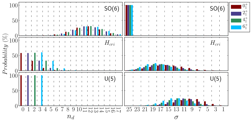
Figure 7: U(5) $n_{d}$-decomposition and SO(6) $\sigma$-decomposition for selected eigenstates of the U(5)-DS Hamiltonian [Fig. 2(a)], the SO(6)-DS Hamiltonian [Fig. 2(b)] and the critical Hamiltonian [Fig. 6(a)].

6 Butterfly catastrophe in the IBM

The cusp catastrophe of Eq. (8) is obtained with SO(5)-invariant one- and two-body terms in the IBM Hamiltonian, and is suitable for describing second order QPTs between spherical and $\gamma$-unstable deformed shapes. In order to accommodate first-order transitions involving a coexistence of such shapes, one needs to have higher powers of $\beta^{2}$ in the Landau potential. This can be accomplished by including higher-order terms in the IBM Hamiltonian. In the present section, we consider the effects of including such cubic terms which conserve the SO(5) symmetry [22]. In this case, the energy surface of Eq. (5) has the form $E_{N}(\beta,\gamma)=N(N-1)(N-2)[z_{0}+E(\beta)]$, where

$$E(\beta)=(1+\beta^{2})^{-3}[\,A\beta^{6}+D\beta^{4}+F\beta^{2}\,]\;\;\;,\;\;\;A>0~{}.$$ (15)

The positive coefficient $A$ can be taken as a scale, hence the surface depends on two essential parameters $D$ and $F$. The extremal points of the surface occur at $\beta=0$ and at

$$\rho_{\pm} = \beta^{2}_{\pm}=\frac{F-D\pm\sqrt{\Delta}}{3A-D}~{},$$ (16a)

$$\Delta = (F-D)^{2}-(3A-D)F~{}.$$ (16b)

The spherical $\beta=0$ extremum is a local minimum (maximum) for $F>0$ ($F<0$) and becomes a global minimum for $F>0$ and $D^{2}-4AF<0$. $\rho_{\pm}$ of Eq. (16a) are solutions of a quadratic equation in the variable $\rho=\beta^{2}$, hence are physically acceptable if positive. When such deformed extrema exist, then $\rho_{+}>0$ ($\rho_{-}>0$) is a local minimum (maximum) and $\rho_{+}>0$ becomes a global minimum for $D^{2}-4AF>0$.

In the terminology of CT, $E(\beta)$ of Eq. (15) corresponds to a butterfly catastrophe with $\beta^{6}$ germ. The phase diagram, shown in Fig. 8, is two-dimensional in the control parameter space $(D,F)$, and involves (I) spherical, (II) deformed and (III) coexistence regions. Region (I) defines the spherical phase, in which the energy surface has as a single minimum at $\beta=0$. It is composed of three sub-regions I(a) ${\textstyle 3A-D<0,F>0}$, [$\rho_{-}\!>\!0$ (max), $\rho_{+}\!<\!0$]; I(b) ${\textstyle 3A-D>0,D\!>F>0,\Delta>0}$, [$\rho_{-}\!<\!\rho_{+}\!<\!0$]; I(c) $\Delta\!<\!0$, [$\rho_{-},\rho_{+}$ complex]. Region (II) defines the deformed phase, in which the energy surface has a single deformed minimum at $\rho_{+}\!>\!0$. It is composed of two sub-regions: II(a) ${\textstyle 3A-D<0,F<0,\Delta>0}$, [$\rho_{-}\!<\!0$, $\rho_{+}\!>\!0$ (min)]; II(b) ${\textstyle 3A-D>0,F<0}$, [$\rho_{-}\!>\!0$ (max), $\rho_{+}\!>\!0$ (min)]; Region (III) defines the coexistence phase, in which the energy surface has both spherical and deformed minima at $\beta\!=\!0$ and $\rho_{+}\!>\!0$, respectively. It is composed of two sub-regions III(a) ${\textstyle 3A-D>0,F>0,\Delta>0,D^{2}-4AF<0}$, and III(b) $D<0,F>0,\Delta>0,D^{2}-4AF>0$, [$\rho_{-}>0$ (max), $\rho_{+}>0$ (min)].

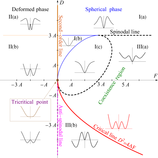
Figure 8: Phase diagram for the butterfly catastrophe (15), composed of (I) spherical, (II) deformed, and (III) coexistence regions, and representative energy curves within each region. The bifurcation set, Eq. (17), and Maxwell set, Eq. (18), separating the different regions, are depicted.

The bifurcation sets are given by

$${\rm Spinodal\,line}\qquad\qquad\;\Delta=0,\;F>D\;;\;D=3A,\;F>D~{},$$ (17a)

$${\rm Anti\!-\!spinodal\,line}\qquad F=0,\;D<0~{},$$ (17b)

$${\rm Second\,order\,line}\qquad\quad F=0,\;D>0~{},$$ (17c)

$${\rm Tricritical\,point}\qquad\quad\;\,F=D=0~{}.$$ (17d)

The Maxwell set defines the critical line

$${\rm Critical\,line}\qquad\quad D^{2}-4AF=0,\quad F>0,\,D<0~{},$$ (18)

along which the critical energy surface acquires the form

$$E_{\rm cri}(\beta)=A(1+\beta^{2})^{-3}\beta^{2}(\beta^{2}-\beta_{0}^{2})^{2}~{},$$ (19)

where $\beta_{0}^{2}\!=\!-D/2A\!=\!-2F/D$. $E_{\rm cri}(\beta)$ has two degenerate minima, at $\beta=0$ and $\beta_{+}^{2}=\beta_{0}^{2}$, and a maximum at $\beta_{-}^{2}=\tfrac{\beta_{0}^{2}}{3+2\beta_{0}^{2}}$. The two minima are separated by a barrier of height $h=A\tfrac{4\beta_{0}^{6}}{27(1+\beta_{0}^{2})}$. The surface landscape is similar to that of Fig. 1(c), and its profile is shown in Fig. 9.

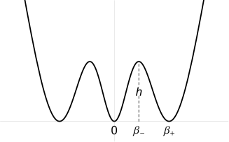
Figure 9: Profile of the critical energy surface $E_{\rm cri}(\beta)$, Eq. (19). $\beta\!=\!0$ and $\beta_{+}$ are two degenerate minima, $E_{\rm cri}(0)\!=\!E_{\rm cri}(\beta_{+})\!=\!0$. The position and height of the barrier are $\beta_{-}$ and $h\!=\!E_{\rm cri}(\beta_{-})$.

The bifurcation and Maxwell sets comprise the separatrix and determine the boundaries of the different regions in the phase diagram of Fig. 8. The spinodal line, Eq. (17a), separates the spherical and coexistence regions. The anti-spinodal line, Eq. (17b), separates the coexistence and deformed regions. The second-order line, Eq. (17c), separates the deformed and spherical regions. The critical line, Eq. (18), partitions the coexistence region to a sub-region III(a), where the spherical (deformed) minimum is global (local), and a sub-region III(b), where the two minima exchange roles. All lines intersect at the tricritical point, Eq. (17d), for which $E(\beta)=A(1+\beta^{2})^{-3}\beta^{6}$.

As the control parameters are varied and the separatrix lines are crossed, the energy surface typography exhibits a qualitative change and a shape-phase transition occurs. From Fig. 8 one sees that across the second-order line, as $F$ increases, a single deformed minimum ($F\!<\!0$) changes continuously into a single spherical minimum ($F\!>\!0$), in accord with a second-order transition. Across the spinodal line, as $D$ decreases, a second local deformed minimum occurs. The two minima become degenerate at the critical line and then cross. The deformed minimum becomes global and the coexistence of the two minima persists until the local spherical minimum disappears at the anti-spinodal line. These are the attributes of a first-order transition. Interestingly, across the anti-spinodal line, as $F$ decreases from positive to negative values, the deformed minimum remains global but $\beta=0$ changes from a local minimum to a maximum, a feature encountered in a second-order transition.

The quantum properties of the butterfly catastrophe can be studied in the IBM, by considering Hamiltonians whose energy surface coincides with that of Eq. (15). Since the latter is sextic, this requires higher-order terms in the Hamiltonian. For that purpose, we extend the one- and two-body Hamiltonian of Eq. (14), by adding to it a cubic term composed of invariant operators of U(5) and SO(6). The resulting Hamiltonian has the form [22],

$$\hat{H}=\epsilon\,\hat{n}_{d}+r\,P^{{\dagger}}_{0}P_{0}+h_{2}\,P^{{\dagger}}_{0}\hat{n}_{d}P_{0}~{}.$$ (20)

Since both SO(5) and SO(3) are preserved by the above Hamiltonian, its eigenstates have good $(\tau,L)$ quantum numbers and can be labeled as $L^{+}_{i,\tau}$, where the ordinal number $i$ enumerates the occurrences of states with the same $(\tau,L)$, with increasing energy.

One of the three parameters in $\hat{H}$ (20) can be taken as a global scale and we set $h_{2}\!=\!1$. The resulting energy surface, Eq. (15), has coefficients: $z_{0}\!=\!\bar{r}$, $A\!=\!1+\bar{\epsilon}$, $D\!=\!-2(1+2\bar{r}-\bar{\epsilon})$ and $F\!=\!1-4\bar{r}+\bar{\epsilon}$, where $\bar{\epsilon}\!=\!\epsilon/(N-1)(N-2)$ and $\bar{r}\!=\!r/(N-2)$ are the essential control parameters. The bifurcation and Maxwell sets of Eqs. (17) and (18), translate into the following conditions on $\bar{\epsilon}$ and $\bar{r}$ (assuming $\bar{r}\geq 0$),

$${\rm Spinodal\,line}\qquad\qquad\;\bar{\epsilon}=\tfrac{1}{3}(1+2\bar{r})^{2}\;\;,\;\;\bar{r}<1~{},$$ (21a)

$${\rm Anti\!-\!spinodal\,line}\qquad\bar{\epsilon}=4\bar{r}-1\;\;,\;\;\bar{r}<1~{},$$ (21b)

$${\rm Second\,order\,line}\qquad\quad\bar{\epsilon}=4\bar{r}-1\;\;,\;\;\bar{r}>1~{},$$ (21c)

$${\rm Tricritical\,point}\qquad\quad\;\,\bar{\epsilon}=3\;\;,\;\;\bar{r}=1~{},$$ (21d)

$${\rm Critical\,line}\qquad\qquad\quad\bar{\epsilon}=\bar{r}(\bar{r}+2)\;\;,\;\;\bar{r}<1~{}.$$ (21e)

In particular, the parameters of the critical Hamiltonian, $\hat{H}_{\rm cri}$, satisfy the condition of Eq. (21e). The corresponding critical surface, $E_{\rm cri}(\beta)$, Eq. (19) and Fig. 9, has a maximum at $\beta_{-}^{2}$ and two degenerate minima at $\beta=0$ and $\beta_{+}^{2}$ separated by a barrier of height $h$, given by

$$\beta_{-}^{2}=\frac{1-\bar{r}}{5+\bar{r}}\;\;\;,\;\;\;\beta_{+}^{2}=\frac{1-\bar{r}}{1+\bar{r}}\;\;\;,\;\;\;h=\frac{2}{27}(1-\bar{r})^{3}~{}.$$ (22)

Small values of $\bar{r}$ ($\bar{r}\to 0$) correspond to a high barrier, while large values ($\bar{r}\to 1$) correspond to a low barrier.

The calculated spectrum of the critical Hamiltonian, $H_{\rm cri}$, for $N=25$, is shown in Fig. 10. The U(5) ($n_{d}$) and SO(6) ($\sigma$) decompositions of selected eigenfunctions are portrayed in Fig. 11. For a low-barrier ($\bar{r}=0.9$), the pattern of energy levels and $E2$ transitions, displayed in Fig. 10(a), resembles an E(5)-like structure (compare with Fig. 6). This interpretation is corroborated for the yrast states, $L^{+}_{1,\tau}$ with $L\!=\!2\tau\!=\!0,2,4,6$, by their $n_{d}$-decomposition shown in Fig. 11(d), and by their $\sigma$-decomposition shown in Fig. 11(b). Both decompositions are seen to be similar to those of the critical “cusp” Hamiltonian (compare with the middle panels of Fig. 7). The $n_{d}$-decomposition for the non-yrast states, $L^{+}_{2,\tau}$ with $L\!=\!2\tau=0,2,4$, shown in Fig. 11(f), displays similar trends.

\begin{overpic}[width=227.62204pt]{fig10a-spec-low-bar-09.pdf} \put(15.0,67.0){(a) Low barrier} \end{overpic}

\begin{overpic}[width=227.62204pt]{fig10b-spec-low-bar-01.pdf} \put(4.0,67.0){(b) High barrier} \end{overpic}

Figure 10: Energy spectra [in units of $E(2^{+}_{1,1})=1$] and $E2$ rates [in units of $B(E2;2^{+}_{1,1}\to 0^{+}_{1,0})=1$] for the critical Hamiltonian, Eq. (20) with parameters as in Eq. (21e) and $N=25$. The $E2$ operator is proportional to $d^{{\dagger}}s+s^{{\dagger}}\tilde{d}$. (a) Low barrier (negligible height), $\bar{r}=0.9$. (b) High barrier, $\bar{r}=0.1$. The barrier’s height is indicated by a horizontal dotted line in the inset.

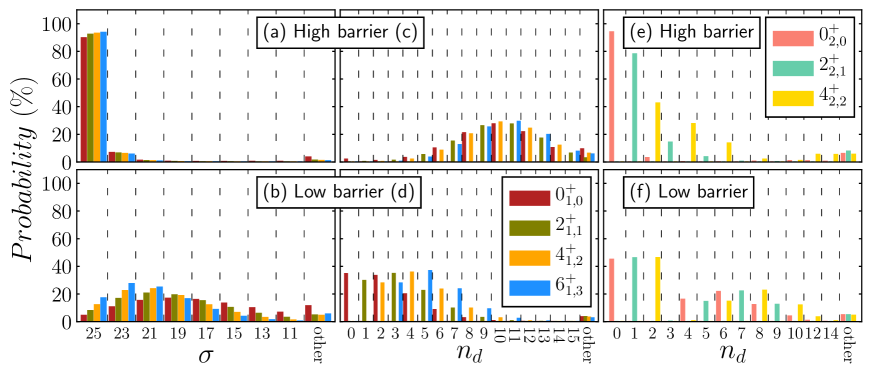
Figure 11: U(5) ($n_{d}$) and SO(6) ($\sigma$) decompositions for selected eigenstates of $\hat{H}_{\rm cri}$ [Fig. 10(a)], appropriate for a low-barrier (bottom row) and [Fig. 10(b)], appropriate for a high-barrier (top row). Panels (a)-(b)-(c)-(d) address yrast states ($L^{+}_{1,\tau}$) and panels (e)-(f) address non-yrast states ($L^{+}_{2,\tau}$).

For a high-barrier ($\bar{r}=0.1$), the spectrum of $\hat{H}_{\rm cri}$ exhibits two distinct classes of states. The first class consists of yrast states, $L^{+}_{1,\tau}$, which form the ground band of a $\gamma$-unstable deformed rotor. As shown in Fig. 10(b), the pattern of energies and $E2$ transitions of these states is similar to that of the SO(6)-DS limit (compare with Fig. 2). The $\sigma$-decomposition shown Fig. 11(a), discloses that these states posses the SO(6) quantum number $\sigma\!=\!N$, to a good approximation. The broad $n_{d}$ distribution shown in Fig 11(c), discloses their deformed nature. These attributes are similar to those encountered in the SO(6)-DS limit (compare with the upper panels of Fig. 7).

The second class consists of non-yrast states, $L^{+}_{2,\tau}$, arranged in $n_{d}$-multiplets of a spherical vibrator. As shown in the inset of Fig. 10(b), the pattern of energies and $E2$ transitions for these states is similar to that of the U(5)-DS limit (compare with Fig. 2). The $n_{d}$-decomposition, shown Fig. 11(e), discloses that their wave functions are dominated by a single $n_{d}$ component (especially, the $0^{+}_{2,0}$ and $2^{+}_{2,1}$ states), similarly to the spherical U(5) basis states (compare with the lower panels of Fig. 7). The fact that for a high barrier, the lowest spherical-type of states show a high degree of purity with respect to U(5) and the lowest deformed-type of states, members of the ground band, show a high degree of purity with respect to SO(6), while other states of the same Hamiltonian are mixed with respect to both U(5) and SO(6), highlights the relevance of partial dynamical symmetries [37, 38] to the spectrum of the critical Hamiltonian. Such a novel symmetry property was encountered in numerous studies of single shapes [37, 38, 39, 40, 41, 42] and multiple shapes [43, 44, 45, 46, 47] in nuclei, and of systems with mixed regular and chaotic dynamics [48, 49, 50].

The evolution of the dynamics along the critical line, from an E(5)-like structure for a low-barrier, to coexisting SO(6)-like and U(5)-like structure for a high barrier, can be investigated by varying the control parameter $\bar{r}$ in the critical Hamiltonian. The results of such a detailed study will be reported elsewhere [22]. A particularly sensitive measure of the height of the barrier is the ratio of $E2$ rates $B(E2;0^{+}_{2,0}\to 2^{+}_{1,1})/B(E2;2^{+}_{1,1}\to 0^{+}_{1,0})$. As indicated in Fig. 10, this ratio is $0.89$ ($0.084$) for $\bar{r}=0.9$ ($\bar{r}=0.1$), i.e., an order-of-magnitude change from low to high barrier.

7 Concluding remarks

We have employed the algebraic framework of the interacting boson model (IBM) for the study of quantum catastrophes. The latter are manifested in first- and second-order QPTs between spherical and $\gamma$-unstable deformed nuclear shapes, whose dynamics is described by the U(5) and SO(6) dynamical symmetries (DSs) of the IBM, respectively.

The classical analysis involves the construction of the Landau potentials by means of coherent states, and the study of the complete phase diagrams by the methods of Catastrophe Theory. The potentials depend on the quadrupole shape variable $\beta$, and on control parameters of the Hamiltonian. A quartic-type of potential exemplifying a cusp catastrophe and a sextic type of potential exemplifying a butterfly catastrophe, have been considered. The relevant bifurcation and Maxwell sets have been identified. The latter mark the boundaries of different regions in the phase diagram, encompassing classes of potentials with similar typography. The crossing of these boundaries corresponds to a shape-phase transition.

The quantum analysis involves a study of the spectra and the structure of wave functions, arising from IBM Hamiltonians which mix terms from two incompatible DS chains. For the cusp catastrophe, one- and two-body interaction terms are sufficient and the Hamiltonian is expanded in terms of the Casimir operators of the leading sub-algebras of the two chains, $\hat{H}(a_{1},a_{2})=a_{1}\,\hat{C}_{k}[G_{1}]+a_{2}\,\hat{C}_{n}[G_{2}]$. For the butterfly catastrophe, a three-body term is required and the Hamiltonian involves a general expansion in terms of invariant operators of ${\rm G_{1}}$ and ${\rm G_{2}}$, $\hat{H}(a_{n,k})=\sum_{n,k}a_{n,k}\,{\cal I}_{n}[G_{1}]\,{\cal I}_{k}[G_{2}]$. In the examples considered, ${\rm G_{1}=U(5)}$ and ${\rm G_{2}=SO(6)}$.

The symmetry-restricted cusp catastrophe is appropriate for a second order QPT. The phase diagram is one-dimensional, involving spherical and deformed regions corresponding to potentials with single minima, and a critical point corresponding to a flat-bottomed quartic potential. The quantum dynamics exhibits a continuous evolution from a U(5) structure to a SO(6) structure, with an E(5)-like structure at the critical point. The symmetry-restricted butterfly catastrophe can accommodate both second- and first-order QPTs. The phase diagram is two-dimensional involving spherical and deformed regions, where the potential has a single minimum, and a coexistence region, where two minima occur in the potential. The quantum dynamics along the critical line, where the two minima are degenerate, displays an evolution from an E(5)-like structure appropriate to a low-barrier to a coexistence of U(5)-like and SO(6)-like structure for a high barrier. A symmetry analysis of the wave functions for the high barrier case, reveals the coexistence of U(5) and SO(6) partial dynamical symmetries. This work is supported by the Israel Science Foundation.

References

References

- [1] Gilmore R 1981 Catastrophe Theory for Scientists and Engineers (New York: Wiley)
- [2] Poston T and Stewart I 1978 Catastrophe Theory and its Applications (London: Pitmman)
- [3] Stewart I 1982 Rep. Prog. Phys. 45 185
- [4] Gilmore R and Feng D H 1978 Nucl. Phys. A 301 189
- [5] Gilmore R 1979 J. Math. Phys. 20 891
- [6] Carr L D Ed 2010 Understanding Quantum Phase Transitions (Boca Raton: CRC Press)
- [7] Sachdev S 1999 Quantum Phase Transitions (Cambridge: Cambridge Univ. Press)
- [8] Cejnar P and Jolie J 2009 Prog. Part. Nucl. Phys. 62 210
- [9] Cejnar P, Jolie J and Casten R F 2010 Rev. Mod. Phys. 82 2155
- [10] Iachello F 2011 Rivista del Nuovo Cimento 34 617
- [11] Gilmore R, Kais S and Levine R D 1986 Phys. Rev. A 34 2442
- [12] Emary C Lambert N and Brandes T 2005 Phys. Rev. A 71 062302
- [13] Cejnar P and Stránský P 2008 Phys. Rev. E 78 031130
- [14] Iachello F and Arima A 1987 The Interacting Boson Model (Cambridge: Cambridge Univ. Press)
- [15] Feng D H, Gilmore R and Deans S R 1981 Phys. Rev. C 23 1254
- [16] López-Moreno E and Castaños O 1996 Phys. Rev. C 54 2374
- [17] García-Ramos J E, Arias J M, Barea J and Frank A 2003 Phys. Rev. C 68 024307
- [18] Cejnar P and Iachello F 2007 J. Phys. A 40, 581
- [19] García-Ramos J E, Arias J M and Dukelsky J 2014 Phys. Lett. B 736 333
- [20] Hellemans V, Van Isacker P, De Baerdemacker S and Heyde K 2007 Nucl. Phys. A 789 164
- [21] García-Ramos J E, Pérez-Fernández P, Arias J M and Freire E 2016 Phys. Rev. C 93 034336
- [22] Gavrielov N and Leviatan A 2020 to be published
- [23] Bohr A and Mottelson B R 1998 Nuclear Structure Vol. II (Singapore: World Scientific)
- [24] Ginocchio J N and Kirson M W 1980 Phys. Rev. Lett. 44 1744
- [25] Dieperink A E L, Scholten O and Iachello F 1980 Phys. Rev. Lett. 44 1747
- [26] Iachello F, Zamfir N V and Casten R F 1998 Phys. Rev. Lett. 81 1191
- [27] Iachello F and Zamfir N V 2004 Phys. Rev. Lett. 92 212501
- [28] Arias J M et al. 2003 Phys. Rev. C 68 041302(R)
- [29] Leviatan A and Ginocchio J N 2003 Phys. Rev. Lett. 90 212501
- [30] Rowe D J 2004 Nucl. Phys. A 745 47
- [31] Dusuel S et al. 2005 Phys. Rev. C 77 011301
- [32] García-Ramos J E, Dukelsky J and Arias J M 2005 Phys. Rev. C 72 037301
- [33] Heinze S, Cejnar P, Jolie J and Macek M 2006 Phys. Rev. C 73 014306
- [34] Macek M, Cejnar P, Jolie J and Heinze S 2006 Phys. Rev. C 73 014307
- [35] Iachello F 2000 Phys. Rev. Lett. 85 3580
- [36] Casten R F and Zamfir N V 2000 Phys. Rev. Lett. 85 3584
- [37] Leviatan A 2011 Prog. Part. Nucl. Phys. 66 93
- [38] Leviatan A 1996 Phys. Rev. Lett. 77 818
- [39] Leviatan A and Sinai I 1999 Phys. Rev. C 60 061301(R)
- [40] García-Ramos J E, Leviatan A and Van Isacker P 2009 Phys. Rev. Lett. 102 112502
- [41] Leviatan A 2012 J. Phys. Conf. Ser. 380 012002
- [42] Leviatan A, García-Ramos J E and Van Isacker P 2013 Phys. Rev. C 87 021302(R)
- [43] Leviatan A 2007 Phys. Rev. Lett. 98 242502
- [44] Leviatan A and Shapira D 2016 Phys. Rev. C 93 051302(R)
- [45] Leviatan A and Gavrielov N 2017 Phys. Scr. 92 114005
- [46] Leviatan A and Gavrielov N 2018 J. Phys. Conf. Ser. 1071 012014
- [47] Leviatan A, Gavrielov N, García-Ramos J E and Van Isacker P 2018 Phys. Rev. C 98 031302(R)
- [48] Whelan N, Alhassid Y and Leviatan A 1993 Phys. Rev. Lett. 71 2208
- [49] Leviatan A and Whelan N D 1996 Phys. Rev. Lett. 77 5202
- [50] Macek M and Leviatan A 2014 Ann. Phys. (N.Y.) 351 302