Stability of electric-field-driven MBL in an interacting long range hopping model

Abstract

We study the fate of many-body localization (MBL) in the presence of long range hopping ($\sim 1/r^{\sigma}$) in a system subjected to an electric field (static and time-periodic) along with a slowly-varying aperiodic potential. We show that the MBL in the static electric-field model is robust against arbitrary long-range hopping in sharp contrast to other disordered models, where MBL is killed by sufficiently long-range hopping. Next, we show that the drive-induced phenomena associated with an ac square wave electric field are also robust against long-range hopping. Specifically, we obtain drive-induced MBL, where a high-frequency drive can convert the ergodic phase into the MBL phase. Remarkably, we find that a coherent destruction of MBL is also possible with the aid of a resonant drive. Thus in both the static and time-periodic square wave electric field models, the qualitative properties of the system are independent of whether the hopping is short-ranged or long-ranged.

I Introduction

Many-body localization (MBL) (Basko et al., 2006; Nandkishore and Huse, 2015; Fleishman and Anderson, 1980; Gornyi et al., 2005), in which localization is known to persist even in the presence of many-body interactions, is a generalization of Anderson localization  (Anderson, 1958). This is characterized by a number of unusual features such as the area law scaling (Bauer and Nayak, 2013) for eigenstates far away from the ground state, logarithmic time-evolution of entanglement entropy (Žnidarič et al., 2008; Bardarson et al., 2012; Serbyn et al., 2013), and violation of the eigenstate thermalization hypothesis (Srednicki, 1994; Rigol et al., 2008). Furthermore, a system in the MBL phase is known to be robust against a high frequency drive in contrast to generic many-body driven systems which tend to a featureless ‘heat death’ (Ponte et al., 2015a; Lazarides et al., 2015; D’Alessio and Polkovnikov, 2013; Abanin et al., 2015; Ponte et al., 2015b; Kozarzewski et al., 2016; Rehn et al., 2016; Gopalakrishnan et al., 2016). Recent advances on the experimental front have also helped to pile up evidence for the MBL phase both in static (Schreiber et al., 2015; Choi et al., 2016; Smith et al., 2016; Kondov et al., 2015; Bordia et al., 2017a) as well as in periodically driven systems (Bordia et al., 2017b).

Although the standard MBL phase is induced by random disorder, systems with non-random potentials are also known to exhibit the MBL phase (Iyer et al., 2013; Lee et al., 2017; Modak and Mukerjee, 2015; Nag and Garg, 2017; Li et al., 2015). A recent proposal to realize MBL-like features in a clean system subjected to a strong electric field and a confining potential (Schulz et al., 2019; van Nieuwenburg et al., 2019; Bhakuni and Sharma, 2020) has created much excitement. Moreover, a time-periodic electric field leads to many counter-intuitive features (Bhakuni et al., 2020; Bairey et al., 2017) such as drive-induced MBL and coherent destruction of Stark-MBL. In this article, we explore the effect of static as well as a time-periodic electric field on an interacting long-range hopping model, and discuss the emergence of the MBL phase in this context.

The study of the MBL phase in the presence of long-range forces has received considerable theoretical interest Khatami et al. (2012); Nandkishore and Sondhi (2017); Singh et al. (2017); Roy and Logan (2019); Gutman et al. (2016); Yao et al. (2014); Tikhonov and Mirlin (2018); Wu and Das Sarma (2016); Nag and Garg (2019); Burin (2006). Long-range forces are ubiquitous in nature; recent technological advances, particularly in dipolar and trapped ionic systems Yao et al. (2014); Smith et al. (2016); Korenblit et al. (2012); Roy et al. (2019), have made the experimental realization of many of these systems, a realistic possibility. In systems with long-range hopping and long-range interactions ($\sim 1/r^{\sigma}$), numerical studies have shown that MBL cannot survive for $\sigma<2$ (Gutman et al., 2016; Yao et al., 2014; Tikhonov and Mirlin, 2018; Wu and Das Sarma, 2016). Recently (Nag and Garg, 2019), it was shown that for a system with a quasi-periodic potential and short-range hopping, the MBL phase is stable for arbitrary long-range interactions. However, long-range hopping partially delocalizes the system for $1<\sigma<2$ and completely delocalizes it for $\sigma<1$. This opens up the question of how general these observations are, and whether a stable MBL phase can be obtained for arbitrary long-range hopping. Another question that springs up, in the backdrop of drive-induced MBL (Bhakuni et al., 2020; Bairey et al., 2017) , is the effect of a time-periodic electric field in the presence of such long-range hopping. Here, we address these questions by studying an interacting long-range hopping model subjected to a (static, and time-periodic) electric field along with a slowly-varying aperiodic potential and find that for suitable parameters, the MBL phase can indeed be obtained for arbitrary long-range hopping.

Our main findings are as follows. For the un-driven model in the short-range hopping case, we find that for small field strength and slowly-varying aperiodic potential, the model shows an ergodic phase. In contrast, for sufficiently large electric field and/or aperiodic potential, the model shows an MBL phase where the nearest-neighbor sites become entangled with each other. The nature of the MBL phase itself seems to depend on whether the electric field or the aperiodic potential is the dominant force. A study of the dynamics shows a faster entanglement entropy growth in the MBL region dominated by the aperiodic potential in comparison to regions where MBL is induced by electric field. This suggests a strong localization by the electric field. This localization remains robust once the long-range hopping is turned on and a stable MBL phase is obtained for a sufficiently large electric field, despite the presence of an arbitrary long-range hopping. Strikingly, when the electric field is converted into a time-dependent square pulse, we obtain both drive-induced MBL and coherent destruction of MBL by a proper tuning of the amplitude and frequency of the drive, even when the hopping is long-ranged.

The organization of the paper is as follows. In Sec. II, we describe the model Hamiltonian along with the various static and dynamical measures to distinguish the ergodic and the MBL phases. In Sec. III, we consider the case of a static electric field and discuss the emergence of the MBL phase in the short-range and long-range hopping limits. In Sec. IV, we discuss the effect of a time-periodic electric field and the phenomenon of drive-induced MBL in the long-range hopping case. Finally, we summarize our main findings in Sec. V.

II Model Hamiltonian and Quantifiers

We consider the Hamiltonian given by

$$H=-\sum_{j>i}^{L-1}J_{ij}(c_{i}^{\dagger}c_{j}+h.c.)+\mathcal{F}(t)\sum_{i=1}^{L}i(n_{i}-\frac{1}{2})$$

$$-\sum_{i=1}^{L}h_{i}(n_{i}-\frac{1}{2})+V\sum_{i=1}^{L-1}(n_{i}-\frac{1}{2})(n_{i+1}-\frac{1}{2}),$$ (1)

where $\mathcal{F}(t)$ is a linear electric field, $V$ is the nearest-neighbor interaction, and $J_{ij}=\frac{J}{|i-j|^{\sigma}}$ is the long-range hopping. Since an additional confining potential is required for Stark-MBL, we perturb the electric field by an additional onsite potential: $h_{i}=h\cos(2\pi\beta i^{n}+\phi)$, where $\beta$ is some irrational number which we set to be the golden mean: $\beta=\frac{\sqrt{5}-1}{2}$ and $\phi\in(-\pi,\pi)$. We also set $n=0.7$, thus making it a slowly-varying aperiodic potential, and adopt the natural units ($a=J=\hbar=e=1$). To ensure the convergence of energy density in the thermodynamic limit, we omit $\sigma<1$ in all the numerical results (Rodríguez et al., 2003; Balagurov et al., 2004; Singh et al., 2017).

The un-driven model is well-understood when it is short-ranged $(\sigma\to\infty)$ and non-interacting $(V=0)$. This becomes a slowly varying aperiodic model for $\mathcal{F}(t)=F=0$, which, for $h<2J$ Sarma et al. (1988, 1990), shows a single particle mobility edge separating the localized and delocalized states. The states between energy $\pm|2J-h|$ are delocalized for $h<2J$, while all single-particle states are localized for $h>2J$. For $h=0$ and $F\neq 0$, we have the well-known Wannier-Stark model in which all the single particle eigenstates are localized and the eigen-spectrum forms an equi-spaced ladder with the spacing proportional to the field strength (Krieger and Iafrate, 1986; Wannier, 1960). As a consequnce of the Wannier-Stark ladder, the dynamics shows Bloch oscillations (Hartmann et al., 2004; Bhakuni and Sharma, 2018; Bhakuni et al., 2019). These oscillations typically dephase in the presence of disorder and non-linearity, however they are known to survive (De Moura et al., 2005) in the presence of a slowly varying ($n<1$) aperiodic potential.

In the presence of interactions $(V\neq 0)$ but short-range hopping, either of electric field or a slowly-varying potential separately can yield both the ergodic and MBL phases for suitable tuning of the field strength and the aperiodic potential (Schulz et al., 2019; van Nieuwenburg et al., 2019; Nag and Garg, 2017). In this paper, we study the combined and relative effect of the electric field and the slowly-varying aperiodic potential together in the presence of many-body interactions. We further explore the scenario where the hopping is made long-ranged and check the stability of the MBL phase. To do so we use the following quantifiers.

II.1 Static measures: level spacing ratio and average nearest-neighbor concurrence

The ergodic and MBL phases can be characterized by the average level spacing ratio, which is defined as (Oganesyan and Huse, 2007; Atas et al., 2013)

$$\langle r\rangle=\langle\frac{\text{min}(\delta_{n},\delta_{n+1})}{\text{max}(\delta_{n},\delta_{n+1})}\rangle,$$ (2)

where, $\delta_{n}=\epsilon_{n+1}-\epsilon_{n}$ is the gap between subsequent energies. In the ergodic phase the average gap ratio approaches the Gaussian orthogonal ensemble (GOE) value: $\langle r\rangle=0.53$ and satisfies Wigner-Dyson statistics whereas in the MBL phase the gap ratio approaches the value : $\langle r\rangle=0.386$ and satisfies Poisson statistics.

Similar to the average level spacing ratio, the average nearest-neighbor concurrence, a measure of entanglement, also uniquely characterizes the ergodic and the MBL phases (Bera and Lakshminarayan, 2016) and can be measured experimentally (Iemini et al., 2016; Fukuhara et al., 2015; Jurcevic et al., 2014). From the two-site reduced density matrix $\rho_{ij}$, the concurrence can be calculated as

$$\mathcal{C}_{ij}=\text{max}(0,\lambda^{(1)}-\lambda^{(2)}-\lambda^{(3)}-\lambda^{(4)}),$$ (3)

where $\lambda^{(i)}$ are the eigenvalues of the matrix $\sqrt{\rho_{ij}\tilde{\rho}_{ij}}$ arranged in the descending order with $\tilde{\rho}_{ij}$ being the spin flip matrix and defined in terms of Pauli spin matrix $\sigma^{y}$ as: $\tilde{\rho}_{ij}=(\sigma^{y}\otimes\sigma^{y})\rho_{ij}^{*}(\sigma^{y}\otimes\sigma^{y})$ (Wootters, 2001; Chang and Wu, 2010). In systems with particle number conservation, the reduced density matrix for the sites $i$ and $j$ reduces to a much simpler form (Nehra et al., 2018; Shu-Sa and Shi-Jian, 2005; Chang and Wu, 2010). Thus the concurrence is given by

$$\mathcal{C}_{ij}=2\text{max}(0,|z_{ij}|-\sqrt{u_{ij}v_{ij}}),$$ (4)

where, $u_{ij}=\langle(1-n_{i})(1-n_{j})\rangle,v_{ij}=\langle n_{i}n_{j}\rangle\ \text{and}\ z_{ij}=\langle c_{j}^{\dagger}c_{i}\rangle$.

Here, we are interested in the entanglement between the nearest-neighbor sites. We define the average nearest neighbor concurrence as: $\mathcal{C}=\frac{1}{(L-1)}\sum_{i=1}^{L-1}\overline{\mathcal{C}}_{i,i+1}$, where the over-bar denotes the average over the central part of the eigen-spectrum. In the ergodic phase, the volume law nature of eigenstates and the principle of monogamy lead to a vanishing nearest-neighbor concurrence while in the MBL phase, the area law nature of the eigenstates together with the monogamy principle lead to a finite concurrence between the nearest-neighbor pairs (Bera and Lakshminarayan, 2016; Iemini et al., 2016; da C Filho et al., 2017).

II.2 Dynamical measures: Entanglement entropy, average concurrence and imbalance

The distinction between the ergodic phase, Anderson localized phase, and MBL phase can also be characterized by the post-quench dynamics of various quantities. To study the dynamics of various observables, we employ the re-orthogonalized Lanczos algorithm (van Nieuwenburg et al., 2019; Luitz and Lev, 2017). Here, we focus on the dynamics of the entanglement entropy, average nearest-neighbor concurrence and the density imbalance starting with an initial state where only the even sites are occupied.

The entanglement entropy is calculated from the density matrix by identifying a subsystem and tracing out the degrees of freedom complementary to it. So, to study its time-evolution, we keep track of the reduced density matrix as a function of time. In the present study, we divide the system into two equal halves with each subsystem having a length of $L/2$. For a given reduced density matrix $\rho_{\text{red}}(t)$, the entanglement entropy can be calculated as: $S(t)=-\text{Tr}[\rho_{\text{red}}(t)\text{ln}\rho_{\text{red}}(t)]$. In the ergodic phase, the growth of entanglement entropy is known to be ballistic in time (barring some exceptions Luitz et al. (2016) that show sub-linear growth) followed by a saturation to its thermal value in the long time  (Kim and Huse, 2013; De Chiara et al., 2006) limit. In the MBL phase, the entanglement growth is unbounded and logarithmic in time for an infinite system, while for finite systems, it saturates to a sub-thermal value. In particular, it has been shown that for the short-ranged XXZ model with weak interactions, the growth of entanglement entropy in the MBL phase is given by (Serbyn et al., 2013) $S(t)\sim\xi\text{ln}(Vt/\hbar)$, where $\xi$ is the single particle localization length.

Similar to the entanglement entropy, the dynamics of two-site entanglement captured by the average concurrence helps identify the different phases. Here, we consider the dynamics of the average nearest-neighbor concurrence defined as: $\mathcal{C}_{NN}^{T}(t)=\frac{1}{(L-1)}\sum_{i=1}^{L-1}\mathcal{C}_{i,i+1}(t)$. The average concurrence is known to decay rapidly in the ergodic phase as the entanglement spreads very fast due to much faster propagation of the quasi-particle excitations. This means that the nearest-neighbor concurrence will vanish rapidly as suggested by the monogamy of entanglement. In the Anderson localized phase, the average concurrence increases for a short time and then saturates, while in the MBL phase, after increase for a short time it shows a power-law decay (Iemini et al., 2016).

Finally, we consider the dynamics of the density imbalance with which signatures of the MBL phase has been obtained experimentally (Schreiber et al., 2015; Bordia et al., 2017a). The density imbalance is defined as

$$\mathcal{I}(t)=\frac{\mathcal{N}_{e}(t)-\mathcal{N}_{o}(t)}{\mathcal{N}_{e}(t)+\mathcal{N}_{o}(t)},$$ (5)

where $\mathcal{N}_{e}(t)$ and $\mathcal{N}_{o}(t)$ are respectively the average number of particles at the even and the odd sites at any instant of time $t$. In the ergodic phase, the imbalance quickly saturates to zero, thus suggesting that it is unable to retain the memory of the initial state. In the MBL phase on the other hand, the imbalance saturates to a non-zero value and retains the memory of the initial state.

III Static Electric field

III.1 MBL in short-range limit $(\sigma\to\infty)$

In the short range limit $(\sigma\to\infty)$, we have an interacting nearest-neighbor hopping model subjected to a static electric field and a slowly varying aperiodic potential. We first consider the average level spacing ratio to characterize the different phases. The value of $\langle r\rangle$ is plotted in Fig. 1(a) as a function of both field strength and the aperiodic potential. An MBL phase is obtained for sufficiently large electric field strength and aperiodic potential. A similar trend can be seen from the average nearest-neighbor concurrence (Fig. 1(c)) which is obtained by averaging over $3000$ eigenstates (for a system of size $L=16$ at half-filling) lying in the central part of the spectrum. The concurrence vanishes in the ergodic phase where the volume law nature of the states implies a vanishingly small entanglement between the neighboring sites. On the other hand, in the MBL phase, the nearest-neighbor pairs acquire a non-zero entanglement.

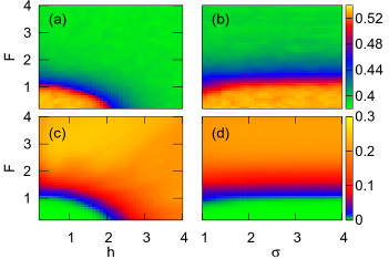
Figure 1: Left panel: (a,c) Surface plot of the average level spacing ratio and average nearest-neighbor concurrence as a function of both field strength and the aperiodic potential for the short-ranged model. Right panel: (b,d) Both level-spacing ratio and average concurrence as a function of field strength and long-range parameter $\sigma$ for a fixed aperiodic potential $h=0.2$. The average nearest-neighbor concurrence is zero in the ergodic phase, while a non-zero average concurrence is obtained for the MBL phase. The other parameters are: $L=16,V=1.0,n=0.7$. For calculating the average nearest-neighbor concurrence, the average is carried out over $3000$ eigenstates from the central part of the spectrum.

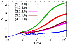
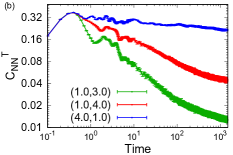
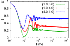
Figure 2: Short-ranged model: The dynamics of $(a)$ entanglement entropy, $(b)$ average nearest-neighbor concurrence, and $(c)$ imbalance for various values of electric field strength and aperiodic potential. The legend shows the value of electric field strength and the strength of aperiodic potential $(F,h)$. Although for all parameters the system is in the MBL phase, the growth of entanglement entropy (and decay of average nearest-neighbor concurrence) is quite different for different points in the MBL phase. The other parameters are: $L=20,V=1.0,n=0.7$. The data are averaged over $100$ configurations of the phase $\phi$.

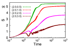
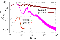
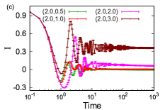
Figure 3: Long-ranged model: The dynamics of $(a)$ entanglement entropy, $(b)$ average nearest-neighbor concurrence, and $(c)$ imbalance for various values of electric field strength and long-range parameter $\sigma$. The legend shows the value of the long range parameter and electric field strength $(\sigma,F)$. The inset in $(b)$ shows the dynamics of average nearest-neighbor concurrence for the parameters in the ergodic phase, where it rapidly decays to zero. The strength of the aperiodic potential is kept fixed at $h=0.2$. The other parameters are: $L=18,V=1.0,n=0.7$. The data are averaged over $100$ configurations of the phase $\phi$.

We then move to the dynamic characterization of the ergodic and MBL phases. The study of dynamics reveals a quantitative difference between the MBL phase obtained from the electric field (plus small aperiodic potential) and the MBL phase obtained from the aperiodic potential (with small field strength). Fig. 2(a) shows the dynamics of entanglement entropy from the aforementioned initial state consisting of alternate filled and empty sites. The plot shows the growth of entanglement entropy (averaged over $100$ different configurations of $\phi$) for the various points ($F,h$) in the MBL phase. It can be seen that for the chosen parameters, the initial (upto $t\approx 1$) growth of the entanglement is the same for all the parameters and after this the entanglement entropy grows logarithmically in time. The MBL phase obtained from the electric field is characterized by a slower logarithmic growth as compared to the MBL phase obtained from the aperiodic potential signifying a stronger localization by the electric field as compared to that by the aperiodic potential.

The dynamics of the average nearest-neighbor concurrence is also plotted in Fig. 2(b). Similar to the entanglement entropy, the initial growth (upto $t\approx 1$) is the same for all the parameters, while it starts to decay as a power-law for longer times. Again, the decay is fast for the points where the MBL is dominated by the aperiodic potential, while it has a slow decay for the MBL dominated by the electric field. Similarly a study of the dynamics of imbalance (Fig. 2(c)) shows that it saturates to a higher value for MBL induced by the electric field as opposed to the aperiodic driven MBL. The dynamical measures provide a hint that MBL induced by electric field can be more robust against any perturbations. We explicitly check this in the next subsection by turning on long-range hopping in the system.

III.2 MBL for long-range hopping

Next, we study the stability of MBL in the presence of arbitrary long-range hopping. Fig. 1(b,d) show the surface plots of the average level spacing ratio and the average nearest-neighbor concurrence respectively as a function of both field strength and the long-range parameter $\sigma$ for a fixed aperiodic potential ($h=0.2$). It can be seen from Fig. 1(b) that for small values of the electric field and all values of the parameter $\sigma$, the level-spacing ratio satisfies Wigner-Dyson statistics and thus signifies an ergodic phase, whereas for large field strength it satisfies Poisson statistics and an MBL phase is indicated. Similarly, the average nearest-neighbor concurrence (Fig. 1(d)) is zero for small values of the electric field and for arbitrary long-range hopping. In contrast, for large electric fields, the average concurrence shows a non-zero value for any arbitrary long-range hopping. It is worth noting that the magnitude of the electric field where the transition between the MBL and ergodic phases happens is almost the same as that of the short-range model (Fig. 1(a,c)). This leads to the conclusion that the MBL induced by the electric field (in the short-range limit) is robust in the presence of arbitrary long-range hopping.

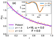
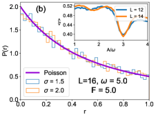
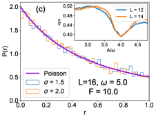
Figure 4: (a-c) Probability distribution of the quasi-energy gap ratio parameter for a high frequency drive ($\omega=5.0$) at the dynamical localization point. The cases:$(a)$ without any static field, $(b)$ resonantly tuned drive ($F=n\omega$) with $n$ odd and $(c)$ resonantly tuned drive with $n$ even are shown. The insets in (a-c) show the average level-spacing ratio (averaged over $100$ configurations of $\phi$) for $\sigma=1.5$, as a function of the ratio $A/\omega$ for different system sizes. In all the cases, the MBL phase is found by tuning the ratio at the dynamical localization point, whereas away from the dynamical localization point an ergodic phase is observed.

We then look at dynamical quantities to characterize the MBL and the ergodic phases. Fig 3(a) shows a plot of the dynamics of the entanglement entropy for $\sigma=2$ and various values of the field strength. After an initial growth, the entanglement entropy saturates to a finite value for small field strengths. The saturation value of the entropy for $F=0.5$ and $L=18$, is $S(t=1000)=5.45$, which is close to the thermal value predicted by Page (Page, 1993) : $S(t\to\infty)=\frac{L}{2}\text{ln}2-0.5$ when the subsystem consists of half of the sites $(L/2)$. For larger field strength $F=3.0$, the entropy displays a slow growth followed by saturation, thus signifying a stable MBL phase for larger field strengths. The average nearest-neighbor concurrence is also plotted in Fig. 3 (b). Again for small field strengths, the average nearest-neighbor concurrence is vanishingly small (inset of Fig. 3(b)), while for larger field strengths it decays as a power-law which supports the argument that for large $F$, a stable MBL phase is observed. Furthermore, the dynamics of the density imbalance also suggests a stable MBL phase for larger field strengths where it saturates to a finite non-zero value. The saturation value decreases on decreasing the field strength where we would expect localization to be less strong.

IV Time-periodic electric field

In this section, we consider a more general electric field that has both dc as well as ac components and restrict to the long-range hopping case. We build on a previous work  (Bhakuni et al., 2020), where we considered the short-range version of a variant Hamiltonian. The electric field can be written as: $\mathcal{F}(t)=F+A\;\text{sgn}(\sin(\omega t))$, where $A$ and $\omega$ respectively are the amplitude and frequency of the ac field, while $F$ is the static dc field. A pure ac square wave drive (with $F=0$ above) yields dynamical localization even in the presence of arbitrary long-range hopping in contrast to sinusoidal driving (Dunlap and Kenkre, 1986; Dignam and de Sterke, 2002), where long-range hopping destroys dynamical localization. We will first consider the non-interacting case, where we obtain the condition for dynamical localization for a combined square wave ac and dc field.

In the absence of both the electric field and the aperiodic potential, the dispersion of the Hamiltonian is given by:

$$E(k)=-2\sum_{m>0}J_{m}\cos mk,$$ (6)

where $J_{m}=1/m^{\sigma}$. When the field is turned on, the quasi-momentum can be written as: $q_{k}(t)=k+Ft+\int_{0}^{t}d\tau F_{ac}(\tau)$, where $F_{ac}$ is the ac part of the field. Due to the dc part, the quasi-momentum is a periodic function only if the resonance condition: $F=n\omega$, holds. Following the same prescription as in the short-ranged model (Bhakuni et al., 2020), the quasi-energy is given as

$$\epsilon(k)=-2\sum_{m>0}J_{m}^{\text{eff}}\cos(mk+\frac{mn\pi}{2}),$$ (7)

where

$$J_{m}^{\text{eff}}=J_{m}\left\{\frac{\sin(\frac{mn\pi}{2}+\frac{mK\pi}{2})}{m(K\pi+n\pi)}+(-1)^{n}\frac{\sin(\frac{mK\pi}{2}-\frac{mn\pi}{2})}{m(K\pi-n\pi)}\right\},$$ (8)

and $K=A/\omega$.

For even and odd $n$ respectively, we get $\epsilon(k)=-2\sum_{m>0}J_{m}^{e}\cos(mk)$ and $\epsilon(k)=-2\sum_{m>0}J_{m}^{o}\sin(mk)$, where

$$J_{m}^{e}=\frac{2J_{m}K\sin(\frac{mK\pi}{2})}{m(K^{2}-n^{2})\pi};\;\;J_{m}^{o}=\frac{2J_{m}K\cos(\frac{mK\pi}{2})}{m(K^{2}-n^{2})\pi}.$$ (9)

Thus the effect of drive in this case is again the renormalization of the hopping parameter. For the even and odd cases respectively, we obtain the condition for dynamical localization by looking at the band collapse points which occur at $K=K_{c}=2\nu$ and $K=K_{c}=2\nu+1$, $\nu$ being any integer and $K_{c}\neq n$. At these points, the band collapse forces an initially localized wave-packet to return to its initial position. However, for other values of $K$, a delocalization effect can be seen due to the band formation. This also provides the mechanism of coherent destruction of Wannier-Stark localization but for an arbitrary long-range hopping.

In the presence of many-body interactions, this dynamical localization is destroyed. However, if an additional small aperiodic potential is present, the MBL phase is obtained close to the dynamical localization point. Fig. 4 shows the probability distribution of the gap-ratio parameter for different values of the static field strength and long-range parameter. In all the cases, the probability distribution matches with that of a Poisson distribution, which suggests the MBL phase at these values. The insets in Fig. 4 show the average gap-ratio as a function of $A/\omega$. It can be seen that only around the dynamical localization point, an MBL phase is obtained, while for other values of $A/\omega$, an ergodic phase is observed. Similar to the short-range case (Bhakuni et al., 2020), the obtained results can be interpreted as follows: for zero dc field and a small aperiodic potential ($h=0.2$), the un-driven model is in the ergodic phase (Fig. 1). The application of a high-frequency drive in this case leads to the MBL phase around the dynamical localization point and an ergodic phase away from the dynamical localization point. This is again a case of drive-induced many-body localization, but for an arbitrary long-range hopping.

Similarly, for a non-zero dc electric field ($F=5.0,10.0$), where the un-driven system is in the MBL phase, the application of a resonant drive can destroy it provided that the ratio $A/\omega$ is tuned away from the dynamical localization point (Fig. 4(b,c)). At the dynamical localization point, the MBL phase is obtained.

V Summary and conclusions

To summarize, we study an interacting long-range hopping model subjected to a general electric field (both ac and dc) and a slowly varying aperiodic potential. We start by studying the short-range hopping case of the undriven model, and find that for small electric field strength and aperiodic potential, the model shows the ergodic phase while for sufficiently large electric field and the aperiodic potential, the model shows the MBL phase. However, the MBL phase obtained by cranking up the electric field is quite different from the MBL phase obtained from large aperiodic potential. While the MBL phase obtained with a large electric field strength and small aperiodic potential shows a slow growth of entanglement entropy, the MBL phase arising from a large aperiodic potential shows a fast growth of entanglement entropy. The distinction becomes even clearer once the hopping is made long-ranged. We find a stable MBL phase for a sufficiently large electric field. This is to be contrasted with the result (Nag and Garg, 2019) that with a dominant quasi-periodic potential, a transition from ergodic to MBL phase is obtained on varying the long-range parameter.

By turning on drive in the long-range hopping model, we obtain generalized conditions for dynamical localization for a combined dc and ac field in the non-interacting limit. In the presence of interactions and small aperiodic potential, we find a high-frequency drive-induced MBL phase for an arbitrary long-range hopping by tuning the system at the dynamical localization point. On the other hand, the drive is also found to take the MBL phase of the un-driven model to the ergodic phase. This shows that the coherent destruction of Stark-MBL is possible, even in the presence of an arbitrary long-range hopping. Thus for both the static and time-periodic square wave electric field, the qualitative behavior of the system are found to be independent of whether the hopping is short-ranged or long-ranged. This fact may help towards the experimental detection of the MBL phase in long-ranged systems.

Appendix A Finite-size flow

In this section, we carry out a finite-size flow analysis of the obtained phases in the main text. We first consider the short-range case. Fig. 5(a) shows the level-spacing ratio as a function of the field strength for a fixed strength of the aperiodic potential $h=0.2$. The finite-size supports the conclusion that an MBL phase is obtained for sufficiently large field strength, while an ergodic phase is obtained for small field strength. Although, the data for different system sizes seem to cross at various points, we suspect this due to a smaller value of the aperiodic potential ($h=0.2$) which is unable to entirely break the many-body degeneracies Schulz et al. (2019) of the problem at very large field strength. To check this explicitly, we present the data for different values of the aperiodic potential ($h=0.5,1.0$, Fig. 5(b,c)) which shows only a single crossing.

We then move to the long-range hopping case with $\sigma=2.0$, and study the variation of the average level-spacing ratio as a function of the field strength with a fixed aperiodic potential ($h=0.2$). Again, finite-size flow suggests an ergodic phase for small field strength and an MBL phase for large field strength (Fig. 6(a)). Finally, we fix the field strength ($F=1.0,3.0$) and vary the long-range parameter $\sigma$ (Fig. 6(b)). The obtained results lead to the conclusion that the Stark-MBL phase is stable for arbitrary long-range hopping.

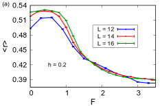
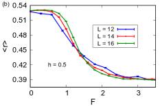
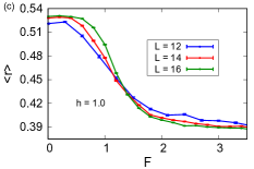
Figure 5: Finite-size flow: (a-c) Average level spacing ratio as a function of the field strength in the short-range limit for $h=0.2,0.5$ and $1.0$ respectively. It can be seen that in all the cases, for small values of the electric field, an ergodic phase is obtained, while for large field strengths an MBL phase is obtained. The data are averaged over $150$ configurations of the phase $\phi$.

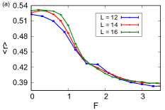
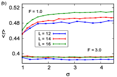
Figure 6: Finite-size flow: (a) Average level spacing ratio as a function of the field strength in the long-range hopping case ($\sigma=2.0$). An MBL phase is obtained only for sufficiently large field strengths. (b) The average level-spacing ratio as a function of the long-range parameter $\sigma$ for $F=1.0,3.0$ and $h=0.2$. An MBL phase is obtained for arbitrary long-range hopping only at sufficiently large field strengths. The data are averaged over $150$ configurations of the phase $\phi$.

Appendix B AAH Limit ($n=1$)

In this section, we consider the limit ($n=1$) where in the absence of the field strength, the non-interacting short-range model becomes the well known Aubry-Andre Harper (AAH) model. Fig. 7 shows the surface plots of the average level spacing ratio for $n=1$, similar to the plots shown in Fig. 1. It can be seen that the qualitative behavior is similar to Fig. 1. This is expected as the electric field dominates over the quasi-periodic potential for small quasi-periodic/aperiodic potential strengths while the qualitative behavior is same for both the quasi-periodic and the aperiodic potential for very high values of $h$.

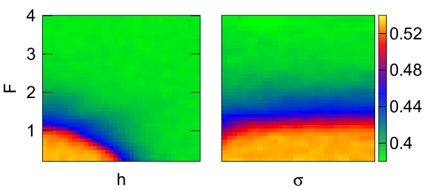
Figure 7: Left: Surface plot of the average level spacing ratio as a function of both field strength and the quasi-periodic potential for the short-ranged model in the AAH limit ($n=1.0$). Right: Surface plot of the average level-spacing ratio as a function of field strength and the long-range parameter for a fixed $h=0.2$. The other parameters are: $L=16,V=1.0,n=1.0$.

References

- Basko et al. (2006) D. M. Basko, I. L. Aleiner, and B. L. Altshuler, Annals of physics 321, 1126 (2006).
- Nandkishore and Huse (2015) R. Nandkishore and D. A. Huse, Annu. Rev. Condens. Matter Phys. 6, 15 (2015).
- Fleishman and Anderson (1980) L. Fleishman and P. W. Anderson, Phys. Rev. B 21, 2366 (1980).
- Gornyi et al. (2005) I. V. Gornyi, A. D. Mirlin, and D. G. Polyakov, Phys. Rev. Lett. 95, 206603 (2005).
- Anderson (1958) P. W. Anderson, Phys. Rev. 109, 1492 (1958).
- Bauer and Nayak (2013) B. Bauer and C. Nayak, Journal of Statistical Mechanics: Theory and Experiment 2013, P09005 (2013).
- Žnidarič et al. (2008) M. Žnidarič, T. Prosen, and P. Prelovšek, Physical Review B 77, 064426 (2008).
- Bardarson et al. (2012) J. H. Bardarson, F. Pollmann, and J. E. Moore, Phys. Rev. Lett. 109, 017202 (2012).
- Serbyn et al. (2013) M. Serbyn, Z. Papić, and D. A. Abanin, Phys. Rev. Lett. 110, 260601 (2013).
- Srednicki (1994) M. Srednicki, Phys. Rev. E 50, 888 (1994).
- Rigol et al. (2008) M. Rigol, V. Dunjko, and M. Olshanii, Nature 452, 854 (2008).
- Ponte et al. (2015a) P. Ponte, A. Chandran, Z. Papić, and D. A. Abanin, Annals of Physics 353, 196 (2015a).
- Lazarides et al. (2015) A. Lazarides, A. Das, and R. Moessner, Physical review letters 115, 030402 (2015).
- D’Alessio and Polkovnikov (2013) L. D’Alessio and A. Polkovnikov, Annals of Physics 333, 19 (2013).
- Abanin et al. (2015) D. A. Abanin, W. De Roeck, and F. Huveneers, Physical review letters 115, 256803 (2015).
- Ponte et al. (2015b) P. Ponte, Z. Papić, F. Huveneers, and D. A. Abanin, Physical review letters 114, 140401 (2015b).
- Kozarzewski et al. (2016) M. Kozarzewski, P. Prelovšek, and M. Mierzejewski, Phys. Rev. B 93, 235151 (2016).
- Rehn et al. (2016) J. Rehn, A. Lazarides, F. Pollmann, and R. Moessner, Phys. Rev. B 94, 020201 (2016).
- Gopalakrishnan et al. (2016) S. Gopalakrishnan, M. Knap, and E. Demler, Phys. Rev. B 94, 094201 (2016).
- Schreiber et al. (2015) M. Schreiber, S. S. Hodgman, P. Bordia, H. P. Lüschen, M. H. Fischer, R. Vosk, E. Altman, U. Schneider, and I. Bloch, Science 349, 842 (2015).
- Choi et al. (2016) J.-y. Choi, S. Hild, J. Zeiher, P. Schauß, A. Rubio-Abadal, T. Yefsah, V. Khemani, D. A. Huse, I. Bloch, and C. Gross, Science 352, 1547 (2016).
- Smith et al. (2016) J. Smith, A. Lee, P. Richerme, B. Neyenhuis, P. W. Hess, P. Hauke, M. Heyl, D. A. Huse, and C. Monroe, Nature Physics 12, 907 (2016).
- Kondov et al. (2015) S. Kondov, W. McGehee, W. Xu, and B. DeMarco, Physical review letters 114, 083002 (2015).
- Bordia et al. (2017a) P. Bordia, H. Lüschen, S. Scherg, S. Gopalakrishnan, M. Knap, U. Schneider, and I. Bloch, Physical Review X 7, 041047 (2017a).
- Bordia et al. (2017b) P. Bordia, H. Lüschen, U. Schneider, M. Knap, and I. Bloch, Nature Physics 13, 460 (2017b).
- Iyer et al. (2013) S. Iyer, V. Oganesyan, G. Refael, and D. A. Huse, Physical Review B 87, 134202 (2013).
- Lee et al. (2017) M. Lee, T. R. Look, S.-P. Lim, and D. Sheng, Physical Review B 96, 075146 (2017).
- Modak and Mukerjee (2015) R. Modak and S. Mukerjee, Physical review letters 115, 230401 (2015).
- Nag and Garg (2017) S. Nag and A. Garg, Physical Review B 96, 060203 (2017).
- Li et al. (2015) X. Li, S. Ganeshan, J. Pixley, and S. D. Sarma, Physical review letters 115, 186601 (2015).
- Schulz et al. (2019) M. Schulz, C. Hooley, R. Moessner, and F. Pollmann, Physical review letters 122, 040606 (2019).
- van Nieuwenburg et al. (2019) E. van Nieuwenburg, Y. Baum, and G. Refael, Proceedings of the National Academy of Sciences 116, 9269 (2019).
- Bhakuni and Sharma (2020) D. S. Bhakuni and A. Sharma, Journal of Physics: Condensed Matter 32, 255603 (2020).
- Bhakuni et al. (2020) D. S. Bhakuni, R. Nehra, and A. Sharma, Phys. Rev. B 102, 024201 (2020).
- Bairey et al. (2017) E. Bairey, G. Refael, and N. H. Lindner, Physical Review B 96, 020201 (2017).
- Khatami et al. (2012) E. Khatami, M. Rigol, A. Relaño, and A. M. García-García, Phys. Rev. E 85, 050102 (2012).
- Nandkishore and Sondhi (2017) R. M. Nandkishore and S. L. Sondhi, Physical Review X 7, 041021 (2017).
- Singh et al. (2017) R. Singh, R. Moessner, and D. Roy, Physical Review B 95, 094205 (2017).
- Roy and Logan (2019) S. Roy and D. E. Logan, SciPost Physics 7 (2019).
- Gutman et al. (2016) D. B. Gutman, I. V. Protopopov, A. L. Burin, I. V. Gornyi, R. A. Santos, and A. D. Mirlin, Phys. Rev. B 93, 245427 (2016).
- Yao et al. (2014) N. Y. Yao, C. R. Laumann, S. Gopalakrishnan, M. Knap, M. Müller, E. A. Demler, and M. D. Lukin, Phys. Rev. Lett. 113, 243002 (2014).
- Tikhonov and Mirlin (2018) K. S. Tikhonov and A. D. Mirlin, Phys. Rev. B 97, 214205 (2018).
- Wu and Das Sarma (2016) Y.-L. Wu and S. Das Sarma, Phys. Rev. A 93, 022332 (2016).
- Nag and Garg (2019) S. Nag and A. Garg, Physical Review B 99, 224203 (2019).
- Burin (2006) A. L. Burin, arXiv preprint cond-mat/0611387 (2006).
- Korenblit et al. (2012) S. Korenblit, D. Kafri, W. C. Campbell, R. Islam, E. E. Edwards, Z.-X. Gong, G.-D. Lin, L.-M. Duan, J. Kim, K. Kim, et al., New Journal of Physics 14, 095024 (2012).
- Roy et al. (2019) N. Roy, A. Sharma, and R. Mukherjee, Physical Review A 99, 052342 (2019).
- Rodríguez et al. (2003) A. Rodríguez, V. Malyshev, G. Sierra, M. Martín-Delgado, J. Rodríguez-Laguna, and F. Domínguez-Adame, Physical review letters 90, 027404 (2003).
- Balagurov et al. (2004) D. Balagurov, V. Malyshev, and F. D. Adame, Physical Review B 69, 104204 (2004).
- Sarma et al. (1988) S. D. Sarma, S. He, and X. Xie, Physical review letters 61, 2144 (1988).
- Sarma et al. (1990) S. D. Sarma, S. He, and X. Xie, Physical Review B 41, 5544 (1990).
- Krieger and Iafrate (1986) J. Krieger and G. Iafrate, Physical Review B 33, 5494 (1986).
- Wannier (1960) G. H. Wannier, Physical Review 117, 432 (1960).
- Hartmann et al. (2004) T. Hartmann, F. Keck, H. Korsch, and S. Mossmann, New Journal of Physics 6, 2 (2004).
- Bhakuni and Sharma (2018) D. S. Bhakuni and A. Sharma, Phys. Rev. B 98, 045408 (2018).
- Bhakuni et al. (2019) D. S. Bhakuni, S. Dattagupta, and A. Sharma, Phys. Rev. B 99, 155149 (2019).
- De Moura et al. (2005) F. De Moura, M. Lyra, F. Domínguez-Adame, and V. Malyshev, Physical Review B 71, 104303 (2005).
- Oganesyan and Huse (2007) V. Oganesyan and D. A. Huse, Physical review b 75, 155111 (2007).
- Atas et al. (2013) Y. Atas, E. Bogomolny, O. Giraud, and G. Roux, Physical review letters 110, 084101 (2013).
- Bera and Lakshminarayan (2016) S. Bera and A. Lakshminarayan, Physical Review B 93, 134204 (2016).
- Iemini et al. (2016) F. Iemini, A. Russomanno, D. Rossini, A. Scardicchio, and R. Fazio, Physical Review B 94, 214206 (2016).
- Fukuhara et al. (2015) T. Fukuhara, S. Hild, J. Zeiher, P. Schauß, I. Bloch, M. Endres, and C. Gross, Phys. Rev. Lett. 115, 035302 (2015).
- Jurcevic et al. (2014) P. Jurcevic, B. P. Lanyon, P. Hauke, C. Hempel, P. Zoller, R. Blatt, and C. F. Roos, Nature 511, 202 (2014).
- Wootters (2001) W. K. Wootters, Quantum Information & Computation 1, 27 (2001).
- Chang and Wu (2010) Z. Chang and N. Wu, Physical Review A 81, 022312 (2010).
- Nehra et al. (2018) R. Nehra, D. S. Bhakuni, S. Gangadharaiah, and A. Sharma, Physical Review B 98, 045120 (2018).
- Shu-Sa and Shi-Jian (2005) D. Shu-Sa and G. Shi-Jian, Chinese Physics Letters 22, 804 (2005).
- da C Filho et al. (2017) J. L. da C Filho, A. Saguia, L. F. Santos, and M. S. Sarandy, Physical Review B 96, 014204 (2017).
- Luitz and Lev (2017) D. J. Luitz and Y. B. Lev, Annalen der Physik 529, 1600350 (2017).
- Luitz et al. (2016) D. J. Luitz, N. Laflorencie, and F. Alet, Phys. Rev. B 93, 060201 (2016).
- Kim and Huse (2013) H. Kim and D. A. Huse, Physical review letters 111, 127205 (2013).
- De Chiara et al. (2006) G. De Chiara, S. Montangero, P. Calabrese, and R. Fazio, Journal of Statistical Mechanics: Theory and Experiment 2006, P03001 (2006).
- Page (1993) D. N. Page, Physical review letters 71, 1291 (1993).
- Dunlap and Kenkre (1986) D. Dunlap and V. Kenkre, Physical Review B 34, 3625 (1986).
- Dignam and de Sterke (2002) M. M. Dignam and C. M. de Sterke, Physical review letters 88, 046806 (2002).