2D Fourier finite element formulation for magnetostatics in curvilinear coordinates with a symmetry direction

Abstract

We present a numerical method for the solution of linear magnetostatic problems in domains with a symmetry direction, including axial and translational symmetry. The approach uses a Fourier series decomposition of the vector potential formulation along the symmetry direction and covers both, zeroth (non-oscillatory) and non-zero (oscillatory) harmonics. For the latter it is possible to eliminate one component of the vector potential resulting in a fully transverse vector potential orthogonal to the transverse magnetic field. In addition to the Poisson-like equation for the longitudinal component of the non-oscillatory problem, a general curl-curl Helmholtz equation results for the transverse problem covering both, non-oscillatory and oscillatory case. The derivation is performed in the covariant formalism for curvilinear coordinates with a tensorial permeability and symmetry restrictions on metric and permeability tensor. The resulting variational forms are treated by the usual nodal finite element method for the longitudinal problem and by a two-dimensional edge element method for the transverse problem. The numerical solution can be computed independently for each harmonic which is favourable with regard to memory usage and parallelisation.

I Introduction

Two-dimensional formulations of electrodynamic problems in translationally and axisymmetric systems are commonly used for numerical treatment by the finite element method [1, 2]. This includes simplified models of three-dimensional systems, as the number of degrees of freedom is substantially reduced compared to the full model. In the simplest case all quantities are assumed to be independent of the symmetry variable, thereby reducing the problem dimension by one. In the more general Fourier finite element method also oscillatory field components are treated by combination of a Fourier expansion in the symmetry coordinate with a numerical solution for each individual harmonic (see, e.g., [3, 4, 5] for the treatment of Maxwell’s equations). For linear problems the Fourier finite element method has the advantage of trivial parallelisability over individual harmonics in comparison to a 3D computation.

Here we treat the magnetostatic problem using the vector potential curl-curl formulation in domains with a symmetry direction, including in particular the translationally and axisymmetric case. Due to the linearity of the curl operator, it is possible to choose a different gauge for each Fourier harmonic and obtain a valid vector potential as the total sum. A similar approach has been taken for the divergence-free interpolation of a given magnetic field in [6]. As a result, the oscillatory part of the curl-curl equation can be treated as a a fully two-dimensional problem using a transverse vector potential. The resulting equations can be viewed as a generalisation of the transverse part of the axisymmetric problem and are in analogy to the transverse formulation of waveguide models [7]. The approach is implemented using the metric-free covariant formulation of Maxwell’s equations in curvilinear coordinates (see [8, 9] for details or [10] for a concise introduction) that is briefly restated in the notation used for further derivations. Here linear constitutive relations contain the permeability tensor represented by its covariant density components implicitly including the influence from curvilinear coordinates via their respective metric tensor. While being mathematically equivalent to the formulation via differential forms the covariant notation remains closer to the traditional formulation via differential operators in flat space. For convenience, Table II lists the relevant designations for both approaches.

Explicit expressions with a scalar permeability are given for the Cartesian case with $2\pi$-periodicity in $z$-direction and axisymmetric systems in cylindrical coordinates. Application to other axisymmetric systems such as spherical, toroidal or symmetry flux coordinates [11] is straightforward by inserting the components of their respective metric tensor. As long as the latter fulfils the necessary requirements, even more exotic coordinate systems (e.g. helical [12]) should be realisable. The resulting variational problems are discretised in coordinate space using a two-dimensional (Nédélec) edge finite element formulation [13, 14] of lowest order for the transverse equations and first order Lagrange elements for the longitudinal non-oscillatory Poisson-like equation. A convergence study for benchmarking problems with existing analytical solutions in an axisymmetric domain is given.

II Derivation of the method

The magnetostatic equations for magnetic field $\bm{{H}}(\bm{{r}})$, magnetic flux density $\bm{{B}}(\bm{{r}})$, and current density $\bm{{J}}(\bm{{r}})$ are

$$\operatorname{\mathbf{curl}}\bm{{H}} =\bm{{J}},$$ (1)

$$\operatorname{div}\bm{{B}} =0,$$ (2)

where $\bm{{H}}$ is related to $\bm{{B}}$ via the constitutive relation

$$\bm{{H}}=\hat{\nu}\bm{{B}}$$ (3)

with local reluctivity (inverse permeability) tensor $\hat{\nu}(\bm{{r}})=\hat{\mu}(\bm{{r}})^{-1}$. Written in terms of a vector potential $\bm{{A}}(\bm{{r}})$ with $\operatorname{\mathbf{curl}}\bm{{A}}=\bm{{B}}$, such that Eq. (2) is automatically fulfilled, they are equivalent to the curl-curl equation,

$$\operatorname{\mathbf{curl}}(\hat{\nu}\operatorname{\mathbf{curl}}\bm{{A}}) =\bm{{J}},$$ (4)

as long as the domain is simply connected.

Our goal is to solve Eq. (4) on a finite three-dimensional domain $\Omega$ with a symmetry direction $\bm{{e}}^{3}=\operatorname{\mathbf{grad}}x^{3}$ along which the cross-section $\Omega_{\mathrm{t}}$ doesn’t change and where all sources and boundary conditions are $2\pi$-periodic in $x^{3}$. An illustration in appropriately ordered cylindrical coordinates $x^{1}=Z$, $x^{2}=R$, $x^{3}=\varphi$ is found in Fig. 1.

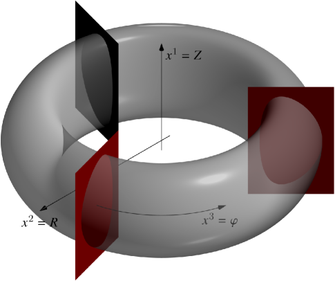
Figure 1: Example of an axisymmetric domain with indication of the coordinate axes for $x^{1},x^{2},x^{3}$. Note that the indicated transverse cross-sections do not change their shape along the symmetry direction $x^{3}$.

II-A Vector calculus in 3D and 2D curvilinear coordinates

Let $(x^{1},x^{2},x^{3})$ be right-handed curvilinear coordinates that uniquely describe any position $\bm{{r}}=\bm{{r}}(x^{1},x^{2},x^{3})$ given by Cartesian components $r^{k}$ in the relevant domain. Co- and contravariant basis vectors are respectively defined by

$$\bm{{e}}_{k}=\frac{\partial\bm{{r}}}{\partial x^{k}}\quad\text{and}\quad\bm{{e}}^{k}=\operatorname{\mathbf{grad}}x^{k},$$ (5)

and co- and contravariant components of vector fields $\bm{{V}}(\bm{{r}})$ by $V_{k}=\bm{{V}}\cdot\bm{{e}}_{k}$ and $V^{k}=\bm{{V}}\cdot\bm{{e}}^{k}$, respectively. Components $g_{ij}$ of the metric tensor $\hat{g}$ are

$$g_{kl}=\bm{{e}}_{k}\cdot\bm{{e}}_{l}=g_{kl}(x^{1},x^{2},x^{3}),$$ (6)

and the metric determinant $g=\det[g_{kl}]$ is always positive, as we are considering right-handed systems. Its square-root $\sqrt{g}$ is equal to the Jacobian of the transformation to Cartesian coordinates and thus the weight of the volume element. The usual symmetry condition $g_{kl}=g_{lk}$ follows from the geometric definition of $\hat{g}$ in Eq. (6).

For the metric-free definition of differential operators and later use in their discretised form for numerics it is useful to introduce densities of weight $W$ to represent scalars, vectors, and tensors. A density $\mathcal{U}$ (denoted in calligraphic letters) of weight $W$ for a quantity $U$ is defined as

$$\mathcal{U}=\sqrt{g}^{W}U,$$ (7)

where $U$ can represent either a scalar, or co/contravariant components of a vector or tensor. If not stated otherwise, we use the term density for the default value $W=+1$. Usual scalars and vector/tensor components correspond to the case $W=0$. Terms such as contravariant vector density and contravariant density representation of a vector will be used synonymously here for easier notation, as the conceptual difference has no practical concequence in the present context.

Table I: Natural input and output for differential operators in curvilinear coordinates, densities are of weight $+1$ here.

Operator	Symbol	Input	Output
Gradient	$\operatorname{\mathbf{grad}}$	scalar	covariant vector
Curl	$\operatorname{\mathbf{curl}}$	covariant vector	contravariant vector density
Divergence	$\operatorname{div}$	contravariant vector density	scalar density
Transverse gradient	$\operatorname{\mathbf{grad}}_{\mathrm{t}}$	scalar	covariant vector
Transverse scalar curl	$\operatorname{curl}_{\mathrm{t}}$	covariant vector	scalar density
Transverse vector curl	$\operatorname{\mathbf{curl}}_{\mathrm{t}}$	scalar	contravariant vector density
Transverse divergence	$\operatorname{div}_{\mathrm{t}}$	contravariant vector density	scalar density

Table II: Translation between terminology of classical tensor calculus and differential geometry in dimension $N$.

Tensor calculus	Differential geometry
scalar	$0$-form / scalar
scalar density	$N$-form
contravariant vector	vector
covariant vector	$1$-form / covector
contravariant vector density	$(N-1)$-form
rank-2 tensor densities	Hodge operators

Table I lists the choice of input and output representation for differential operators such that the Jacobian $\sqrt{g}$ is formally removed from their definition. In this way, the coordinate-independent definitions of 3D divergence and gradient are

$$\operatorname{div}\bm{{U}}=\partial_{k}\mathcal{U}^{k},\quad\operatorname{\mathbf{grad}}U=\bm{{e}}^{k}\partial_{k}U,$$ (8)

where the divergence acts on a contravariant vector density and yields a scalar density, and the gradient acts on a scalar field and yields a covariant vector field. The 3D curl operator

$$\operatorname{\mathbf{curl}}\bm{{U}}=\epsilon^{ijk}\bm{{e}}_{i}\partial_{j}U_{k}$$

acts on a covariant vector field and yields a contravariant vector density. It contains the Levi-Civita tensor $\hat{\epsilon}$ with contravariant density components $\epsilon^{ijk}=1$ for $ijk$ being circular permutations of $123$, $-1$ for permutations of $321$, and $0$ otherwise.

We want to treat the symmetry direction $x^{3}$ separately, splitting the problem into a longitudinal part along the symmetry direction, and a transverse part containing the remaining two dimensions. For the notation of two-dimensional vectors we use lowercase bold letters, i.e.

$$\bm{{u}}=U_{1}\bm{{e}}^{1}+U_{2}\bm{{e}}^{2}=U^{1}\bm{{e}}_{1}+U^{2}\bm{{e}}_{2}.$$

We define two-dimensional transverse divergence and gradient operators analogous to the 3D case with

$$\operatorname{div}_{\mathrm{t}}\bm{{u}}=\partial_{1}\mathcal{U}^{1}+\partial_{2}\mathcal{U}^{2},\quad\operatorname{\mathbf{grad}}_{\mathrm{t}}U=\bm{{e}}^{1}\partial_{1}U+\bm{{e}}^{2}\partial_{2}U.$$ (9)

For the curl, in contrast to 3D, both a vectorial and a scalar transverse curl operator exist with

$$\operatorname{\mathbf{curl}}_{\mathrm{t}}U\bm{{e}}_{1}\partial_{2}U-\bm{{e}}_{2}\partial_{1}U,\quad\bm{{u}}=\partial_{1}U_{2}-\partial_{2}U_{1},$$ (10)

yielding vector and scalar densities, respectively. Note that all four of these operations either take a scalar corresponding to the longitudinal part as input and give a two-dimensional vector corresponding to the transverse part as output, or vice versa.

Matching input and output of operators in Table I reflect the de Rham complex [14] describing in which order operators may act between different function spaces. In 3D this is

$$H^{1}\overset{\operatorname{\mathbf{grad}}}{\rightarrow}H^{\operatorname{\mathbf{curl}}}\overset{\operatorname{\mathbf{curl}}}{\rightarrow}H^{\operatorname{div}}\overset{\operatorname{div}}{\rightarrow}L^{2},$$ (11)

where application of two operators in a row yields zero, e.g. $\operatorname{\mathbf{curl}}\operatorname{\mathbf{grad}}U=0$. This is the case for any de Rham complex. The 3D de Rham diagram leads from a scalar field in $H^{1}$ to a scalar density field in $L^{2}$.

Since the curl operator mixes vector components and to distinguish between transverse and longitudinal parts, relation (11) breaks up into two separate ones in 2D, given by

$$H^{1}\overset{\operatorname{\mathbf{grad}}_{\mathrm{t}}}{\rightarrow}H^{\operatorname{curl}_{\mathrm{t}}}\overset{\operatorname{curl}_{\mathrm{t}}}{\rightarrow}L^{2},$$ (12)

$$H^{1}\overset{\operatorname{\mathbf{curl}}_{\mathrm{t}}}{\rightarrow}H^{\operatorname{div}_{\mathrm{t}}}\overset{\operatorname{div}_{\mathrm{t}}}{\rightarrow}L^{2}.$$ (13)

As in 3D, both diagrams lead from a scalar field in $H^{1}$ to a scalar density field in $L^{2}$. The difference lies in the use of covariant vectors in $H^{\operatorname{curl}_{\mathrm{t}}}$ or contravariant vector densities in $H^{\operatorname{div}_{\mathrm{t}}}$. These two cases can be translated into each other by rotation via the 2D Levi-Civita tensor $\hat{\epsilon}_{\mathrm{t}}$ with contravariant density components given by

$$\epsilon_{\mathrm{t}}^{kl}=\begin{pmatrix}0&1\\ -1&0\end{pmatrix}.$$ (14)

Relations between 2D differential operators can be written as

$$\operatorname{\mathbf{curl}}_{\mathrm{t}}U =\hat{\epsilon}_{\mathrm{t}}\operatorname{\mathbf{grad}}_{\mathrm{t}}U,$$ (15)

$$\operatorname{curl}_{\mathrm{t}}\bm{{u}} =\operatorname{div}_{\mathrm{t}}(\hat{\epsilon}_{\mathrm{t}}\bm{{u}}).$$ (16)

II-B Covariant formulation of classical electrodynamics

Using differential operators in the metric-free way stated above, Maxwell’s equations act on density representations of fields listed in Table III. In SI units they are written as

$$\partial_{k}\mathcal{D}^{k} =\varrho,$$ (17)

$$\epsilon^{ijk}\partial_{j}E_{k} =-\frac{\partial\mathcal{B}^{i}}{\partial t},$$ (18)

$$\epsilon^{ijk}\partial_{j}H_{k} =\mathcal{J}^{i}+\frac{\partial\mathcal{D}^{i}}{\partial t},$$ (19)

$$\partial_{k}\mathcal{B}^{k} =0,$$ (20)

in any curvilinear coordinate system. Magnetostatic equations (1-2) are reproduced in the stationary limit of (19–20) with vanishing time derivatives. The constitutive relations linking excitations $\mathcal{D}^{k},H_{k}$ to local linear responses $E_{l},\mathcal{B}^{l}$ are

$$\mathcal{D}^{k} =\varepsilon^{kl}E_{l},$$ (21)

$$H_{k} =\nu_{kl}\mathcal{B}^{l},$$ (22)

with permittivity $\hat{\varepsilon}$ and reluctivity $\hat{\nu}$ respectively represented by contravariant $W=+1$ density and covariant $W=-1$ density components,

$$\varepsilon^{kl} =\sqrt{g}\bm{{e}}^{k}\cdot\hat{\varepsilon}\bm{{e}}^{l},$$ (23)

$$\nu_{kl} =\sqrt{g}^{-1}\bm{{e}}_{k}\cdot\hat{\nu}\bm{{e}}_{l}.$$ (24)

While the field equations (17–20) remain coordinate-independent, Eqs. (21–22) contain all influence from the metric tensor $\hat{g}$ implicitly via the basis vectors and the Jacobian in Eqs. (23–24). In particular for a scalar $\nu$, components of $\hat{g}$ enter the resulting covariant density representation of $\hat{\nu}$ in curvilinear coordinates,

$$\nu_{kl}=\frac{1}{\sqrt{g}}\sum_{i,j}\partial_{k}r^{i}\partial_{l}r^{j}\nu\delta_{ij}=\frac{g_{kl}}{\sqrt{g}}\nu.$$ (25)

This means that covariant reluctivity components generated by a scalar $\nu$ inherit their symmetry properties from $g_{kl}$. If physical components of the permeability tensor are already given in the desired coordinate frame as a matrix $[\mu_{(kl)}]$, covariant density components of $\hat{\nu}$ can be found by taking its inverse $[\nu_{(kl)}]=[\mu_{(kl)}]^{-1}$ and computing

$$\nu_{kl}=\frac{\sqrt{g_{kk}g_{ll}}}{\sqrt{g}}\nu_{(kl)}.$$ (26)

One can see that if $\nu_{kl}$ are constant in certain curvilinear coordinates, physical components $\nu_{(kl)}$ will usually vary locally and vice-versa. One should remark that the solution for covariant components $H_{k}$ in curvilinear geometry with constant physical $\nu_{(kl)}$ is identical to one for Cartesian components of $\bm{{H}}$ with a spatially varying $\nu_{(kl)}$. Thus one could emulate curvilinear geometry for magnetostatics in flat geometry by a material with locally varying permeability, and vice versa.

Table III: Conventions to represent electromagnetic scalar, vector and tensor fields by densities of varying weight.

Quantity	Symbol	Representation	Weight
Metric tensor	$g_{kl}$	covariant	$0$
Inverse metric	$g^{kl}$	contravariant	$0$
Jacobian	$\sqrt{g}$	scalar	$+1$
Levi-Civita tensor	$\epsilon^{ijk}$	contravariant	$+1$
Charge density	$\varrho$	scalar	$+1$
Current density	$\mathcal{J}^{k}$	contravariant	$+1$
Electric field	$E_{k}$	covariant	$0$
Magnetic flux density	$\mathcal{B}^{k}$	contravariant	$+1$
Electric displacement	$\mathcal{D}^{k}$	contravariant	$+1$
Magnetic field	$H_{k}$	covariant	$0$
Scalar potential	$\Phi$	scalar	$0$
Vector potential	$A_{k}$	covariant	$0$
Permittivity	$\varepsilon^{kl}$	contravariant	$+1$
Permeabiliy	$\mu^{kl}$	contravariant	$+1$
Reluctivity	$\nu_{kl}$	covariant	$-1$
Longitudinal reluctivity	$\nu_{33}$	scalar	$-1$
Transverse reluctivity	$\nu_{\mathrm{t},\,kl}$	covariant	$-1$
Mod. transv. reluctivity	$\bar{\nu}_{\mathrm{t}}^{kl}$	contravariant	$+1$
Transverse Levi-Civita tensor	$\epsilon_{\mathrm{t}}^{kl}$	contravariant	$+1$

II-C Reduction of magnetostatics to 2D by Fourier expansion

To reduce the 3D problem of Eq. (4) to a number of 2D equations we write quanties assumed to be $2\pi$-periodic in $x^{3}$ as a Fourier series

$$f(x^{1},x^{2},x^{3})=\sum_{n=-\infty}^{\infty}f_{n}(x^{1},x^{2})\,e^{\mathrm{i}nx^{3}}.$$ (27)

The following equations concern single harmonics with $n$ omitted as an index in the notation. To be compatible with the curl-curl equation (4) in covariant form we require a Fourier expansion of covariant vector components $A_{k}$ of $\bm{{A}}$ and contravariant vector density components $\mathcal{J}^{k}$ of $\bm{{J}}$.

To retain linearity of terms involving $x^{3}$ and thus avoid mode-coupling via convolution in the constitutive relation (22), we require covariant $W=-1$ density components $\nu_{kl}=\nu_{kl}(x^{1},x^{2})$ of the impermebility tensor $\hat{\nu}$ to be independent of the symmetry coordinate $x^{3}$ if we allow arbitrary harmonics $n$ for the fields. In addition, to be able to split transverse and longitudinal components of fields later, off-diagonal components in $x^{3}$ shall vanish. This means that

$$\nu_{kl}=\begin{pmatrix}\nu_{\mathrm{t},\,kl}&\begin{array}[]{c}0\\ 0\end{array}\\ \begin{array}[]{cc}0&0\end{array}&\nu_{33}\end{pmatrix},$$ (28)

with transverse reluctivity

$$\nu_{\mathrm{t},\,kl}=\begin{pmatrix}\nu_{11}&\nu_{12}\\ \nu_{21}&\nu_{22}\end{pmatrix}$$ (29)

as a covariant $W=-1$ density and longitudinal reluctivity $\nu_{33}$ as a scalar $W=-1$ density. In the case of a scalar permeability, those symmetry restrictions thus apply to the metric tensor and vice versa, so $\sqrt{g}^{-1}g_{kl}$ shall be independent from $x^{3}$ and $g_{k3}=g_{3k}=0$ for $k\neq 3$. A modified transverse reluctivity

$$\hat{\bar{\nu}}_{\mathrm{t}}=-\hat{\epsilon}_{\mathrm{t}}\hat{\nu}_{\mathrm{t}}\hat{\epsilon}_{\mathrm{t}}$$ (30)

is useful to introduce, with contravariant density components

$$\bar{\nu}_{\mathrm{t}}^{kl}=\begin{pmatrix}\nu_{22}&-\nu_{21}\\ -\nu_{12}&\nu_{11}\end{pmatrix},$$

proportional to the transpose of the inverse of (29). For a scalar $\nu$ and $g_{kl}$ of the form (28) this reduces to

$$\bar{\nu}_{\mathrm{t}}^{kl}=\frac{\sqrt{g}\,g_{\mathrm{t}}^{kl}}{g_{33}}\nu,$$ (31)

where $g_{\mathrm{t}}^{kl}$ is the transverse part of the (symmetric) inverse metric tensor.

Under the given restrictions the non-oscillatory part $n=0$ of Eq. (4) splits into a transverse and a longitudinal part with

$$\operatorname{\mathbf{curl}}_{\mathrm{t}}\nu_{33}\operatorname{curl}_{\mathrm{t}}\bm{{a}} =\bm{{j}},$$ (32)

$$\operatorname{curl}_{\mathrm{t}}\hat{\nu}_{\mathrm{t}}\operatorname{\mathbf{curl}}_{\mathrm{t}}A_{3} =\mathcal{J}^{3},$$ (33)

where two-component $\bm{{a}}=A_{1}\bm{{e}}^{1}+A_{2}\bm{{e}}^{2}$ are expressed as a covariant vector and $\bm{{j}}=\mathcal{J}^{1}\bm{{e}}_{1}+\mathcal{J}^{2}\bm{{e}}_{2}$ as a contravariant vector density. The labels transverse for Eq. (32) and longitudinal for Eq. (33) refer to $\bm{{A}}$ and $\bm{{J}}$ here. This is not to be confused with $\bm{{B}}$ itself, for which exactly the opposite is the case, i.e. the longitudinal $\mathcal{B}^{3}$ follows from Eq. (32) and the transverse $\bm{{b}}$ from Eq. (33), corresponding to the first step in Eq. (12) and (13), respectively. Using the relations between 2D differential operators in Eqs. (15-16) together with the modified transverse reluctivity $\hat{\bar{\nu}}_{\mathrm{t}}$ of Eq. (30), we can re-write Eq. (33) as

$$-\operatorname{div}_{\mathrm{t}}(\hat{\bar{\nu}}_{\mathrm{t}}\operatorname{\mathbf{grad}}_{\mathrm{t}}A_{3})=\mathcal{J}^{3}.$$ (34)

For the oscillatory part with $n\neq 0$, we set the covariant component $A_{3}$ to zero by a gauge transformation

$$\bm{{A}}\rightarrow\bm{{A}}-\operatorname{\mathbf{grad}}\int_{x_{0}^{3}}^{x^{3}}A_{3}\,\mathrm{d}x^{3\prime}.$$ (35)

This corresponds to setting $\bm{{A}}\rightarrow\bm{{A}}-\operatorname{\mathbf{grad}}A_{3}/(\mathrm{i}n)$ for single harmonic $\bm{{A}}=\bm{{A}}_{n}(x_{1},x_{2})e^{\mathrm{i}nx^{3}}$ with harmonic index $n$. Independent gauging in that manner is possible for each $n\neq 0$. Due to the superposition principle, we can use a fully transverse vector potential with a different gauge for each individual harmonic and take a Fourier sum in the end. In that case the contravariant magnetic flux density components are given by

$$\mathcal{B}^{1}=-\mathrm{i}nA_{2},\quad\mathcal{B}^{2}=\mathrm{i}nA_{1},\quad\mathcal{B}^{3}=\operatorname{curl}_{\mathrm{t}}\bm{{a}}.$$ (36)

Ampère’s law is transformed to

$$\partial_{2}(\nu_{33}\operatorname{curl}_{\mathrm{t}}\bm{{a}})+n^{2}(\nu_{22}A_{1}-\nu_{21}A_{2}) =\mathcal{J}^{1},$$ (37)

$$-\partial_{1}(\nu_{33}\operatorname{curl}_{\mathrm{t}}\bm{{a}})+n^{2}(-\nu_{12}A_{1}+\nu_{11}A_{2}) =\mathcal{J}^{2},$$ (38)

$$\mathrm{i}n\left[\partial_{1}(\nu_{22}A_{1}-\nu_{21}A_{2})+\partial_{2}(\nu_{11}A_{2}-\nu_{12}A_{1})\right] =\mathcal{J}^{3}.$$ (39)

Eqs. (37-38) contain only transverse components of $\bm{{A}}$ and $\bm{{J}}$ and can be rewritten by using the vector $\operatorname{\mathbf{curl}}_{\mathrm{t}}$ operator, yielding the purely 2D problem for $n\neq 0$ as

$$\operatorname{\mathbf{curl}}_{\mathrm{t}}\left(\nu_{33}\operatorname{curl}_{\mathrm{t}}\bm{{a}}\right)+n^{2}\hat{\bar{\nu}}_{\mathrm{t}}\bm{{a}}=\bm{{j}}.$$ (40)

As opposed to the singular ungauged three-dimensional curl-curl equation (32), the additional term resulting from the fixed gauge makes Eq. (40) uniquely solveable, analogous to the 3D curl-curl equation with a time-harmonic term. Like in the scalar Helmholtz equation $-\upDelta\Phi+n^{2}\Phi=\rho$ arising from Fourier expansion of the Poisson equation, the positive sign of the term weighted by $n^{2}$ leads to rapidly decaying solutions, opposed to oscillating solutions which would typically result from the Fourier expansion of a wave equation in time. Eq. (39) links longitudinal $\bm{J}$ and $\bm{B}$ components and can be written compactly as

$$\mathrm{i}n\operatorname{div}_{\mathrm{t}}(\hat{\bar{\nu}}_{\mathrm{t}}\bm{{a}})=\mathcal{J}^{3}.$$ (41)

Eq. (41) is automatically fulfilled via the divergence relation for Fourier harmonics

$$\operatorname{div}_{\mathrm{t}}\bm{{j}}+\mathrm{i}n\mathcal{J}^{3}=0,$$ (42)

which can be seen from applying $\operatorname{div}_{\mathrm{t}}$ to Eq. (40).

Formally, by setting $n=0$, Eq. (40) includes Eq. (32) as a special case, so we summarize the two as the class of transverse equations (40) for arbitrary $n$, whereas the longitudinal equation (34) equivalent to Eq. (33) needs only to be solved for $n=0$.

II-D Variational formulation in coordinate space

To find a variational formulation for numerical computations, Eqs. (34) and (40) are multiplied by a test function and integrated with weight $\sqrt{g}$ in coordinate space $(x^{1},x^{2})$ parametrising the cross-section perpendicular to the symmetry direction of the original domain $\Omega$ with a 2D volume element $\mathrm{d}\Omega_{\mathrm{t}}:=\mathrm{d}x^{1}\,\mathrm{d}x^{2}$ and line element on the boundary,

$$\mathrm{d}\Gamma_{\mathrm{t}}=\sqrt{\left(\mathrm{d}x^{1}\right)^{2}+\left(\mathrm{d}x^{2}\right)^{2}}.$$ (43)

Volume integration of quantities $F(x^{1},x^{2})$ over $\Omega$ and dividing the result by the range $2\pi$ of $x^{3}$ results in an integral over $\Omega_{\text{t}}$ of the density representation $\mathcal{F}=\sqrt{g}F$,

$$\begin{split}\frac{1}{2\pi}\int_{\Omega}F(x^{1},x^{2})\,\mathrm{d}V=\frac{1}{2\pi}\int_{0}^{2\pi}\mathrm{d}x^{3}\int_{\Omega_{\mathrm{t}}}\mathrm{d}x^{1}\,\mathrm{d}x^{2}\,\mathcal{F}(x^{1},x^{2})=\int_{\Omega_{\mathrm{t}}}\mathcal{F}(x^{1},x^{2})\,\mathrm{d}\Omega_{\mathrm{t}}.\end{split}$$ (44)

The variational form of the longitudinal equation (34) for the non-oscillatory part $n=0$ with scalar test function $w(x^{1},x^{2})$ is

$$\begin{split}\int_{\Omega_{\mathrm{t}}}(\partial_{k}w)\bar{\nu}_{\mathrm{t}}^{kl}(\partial_{l}A_{3})\,\mathrm{d}\Omega_{\mathrm{t}}-\int_{\Gamma_{\mathrm{t}}}wn_{k}\bar{\nu}_{\mathrm{t}}^{kl}(\partial_{l}A_{3})\,\mathrm{d}\Gamma_{\mathrm{t}}=\int_{\Omega_{\mathrm{t}}}w\mathcal{J}^{3}\,\mathrm{d}\Omega_{\mathrm{t}}.\end{split}$$ (45)

Here $\bm{{n}}=(n_{1},n_{2})$ is the unit outward normal vector across the boundary line $\Gamma_{\mathrm{t}}$ in coordinate space $(x^{1},x^{2})$ and the implied sums are taken over $k,l$ from $1$ to $2$. For the special case $w=1$ a compatibility condition follows as

$$-\int_{\Gamma_{\mathrm{t}}}n_{k}\bar{\nu}_{\mathrm{t}}^{kl}\partial_{l}A_{3}\,\mathrm{d}\Gamma_{\mathrm{t}}=\int\mathcal{J}^{3}\,\mathrm{d}\Omega_{\mathrm{t}},$$ (46)

fixing the Neumann term in Eq. (45) corresponding to the magnetic field parallel to the transverse boundary to the total current through the surface $x^{3}=\mathrm{const.}$ within the domain.

For the transverse equation (40), with vectorial test function $\bm{{w}}$ and denoting the coordinate vector along the boundary in counter-clockwise direction by $\bm{{s}}=(s^{1},s^{2})=-\hat{\epsilon}_{\mathrm{t}}\bm{{n}}=(-n_{2},n_{1})$, we obtain

$$\begin{split}\int_{\Omega_{\mathrm{t}}}\operatorname{curl}_{\mathrm{t}}\bm{{w}}\,\nu_{33}\operatorname{curl}_{\mathrm{t}}\bm{{a}}\,\mathrm{d}\Omega_{\mathrm{t}}+n^{2}\int_{\Omega_{\mathrm{t}}}w_{k}\bar{\nu}_{\mathrm{t}}^{kl}A_{l}\,\mathrm{d}\Omega_{\mathrm{t}}-\int_{\Gamma_{\mathrm{t}}}w_{k}s^{k}\nu_{33}\operatorname{curl}_{\mathrm{t}}\bm{{a}}\,\mathrm{d}\Gamma_{\mathrm{t}}=\int_{\Omega_{\mathrm{t}}}w_{k}\mathcal{J}^{k}\,\mathrm{d}\Omega_{\mathrm{t}},\end{split}$$ (47)

for the case $n=0$ as well as $n\neq 0$.

II-E Cartesian and cylindrical coordinates

For Cartesian coordinates and scalar reluctivity $\nu$, the variational form of Eq. (47) with Neumann boundary condition on $\Gamma_{\mathrm{t}}$ and test function $\bm{{w}}$ is given by

$$\begin{split}\int_{\Omega_{\mathrm{t}}}\operatorname{curl}_{\mathrm{t}}\bm{{w}}\,\nu\operatorname{curl}_{\mathrm{t}}\bm{{a}}\,\mathrm{d}x\,\mathrm{d}y+n^{2}\int_{\Omega_{\mathrm{t}}}\bm{{w}}\cdot\nu\bm{{a}}\,\mathrm{d}x\,\mathrm{d}y{}-\int_{\Gamma_{\mathrm{t}}}\bm{{s}}\cdot\bm{{w}}\nu\operatorname{curl}_{\mathrm{t}}\bm{{a}}\,\mathrm{d}\Gamma=\int_{\Omega_{\mathrm{t}}}\bm{{w}}\cdot\bm{{j}}\,\mathrm{d}x\,\mathrm{d}y.\end{split}$$ (48)

Here, $\bm{{s}}=(-n_{y},n_{x})$ is the tangential vector along the boundary line $\Gamma_{\mathrm{t}}$ of the $xy$ cut of the domain, $\Omega_{\mathrm{t}}$, and $\bm{{n}}=(n_{x},n_{y})$ the unit outward normal vector orthogonal to $\bm{{s}}$ in this cross-section.

For cylindrical coordinates $x^{1}=Z,\,x^{2}=R,\,x^{3}=\varphi$, the non-vanishing metric components are $g_{11}=g_{22}=1$ and $g_{33}=R^{2}$ and Eq. (47) with a scalar permeability $\nu$ yields

$$\begin{split}\int_{\Omega_{\mathrm{t}}}(\partial_{Z}w_{R}-\partial_{R}w_{Z})R\nu(\partial_{Z}A_{R}-\partial_{R}A_{Z})\,\mathrm{d}R\,\mathrm{d}Z+n^{2}\int_{\Omega_{\mathrm{t}}}\frac{\nu}{R}(w_{R}A_{R}+w_{Z}A_{Z})\,\mathrm{d}R\,\mathrm{d}Z\\ -\int_{\Gamma_{\mathrm{t}}}(w_{R}s^{R}+w_{Z}s^{Z})R\nu(\partial_{Z}A_{R}-\partial_{R}A_{Z})\,\mathrm{d}\Gamma_{\mathrm{t}}=\int_{\Omega_{\mathrm{t}}}(w_{R}\mathcal{J}^{R}+w_{Z}\mathcal{J}^{Z})\,\mathrm{d}R\,\mathrm{d}Z.\end{split}$$ (49)

III Finite element discretisation

For the general transverse variational problem in Eq. (47), the natural discretisation for $\bm{{a}}$ are 2D (Nédélec) edge elements conforming to $H(\operatorname{\mathbf{curl}},\Omega_{\mathrm{t}})$. Due to its fixed divergence in Eq. (33), components $\mathcal{J}^{k}$ of the transverse current density $\bm{{j}}$ should be discretized by 2D (Raviart-Thomas) elements conforming to $H(\operatorname{div},\Omega_{\mathrm{t}})$. For practical reasons, it is convenient to define a quantity $\bm{{t}}$ in $H(\operatorname{\mathbf{curl}},\Omega_{\mathrm{t}})$ with $\operatorname{div}_{\mathrm{t}}\bm{{j}}=\operatorname{curl}_{\mathrm{t}}\bm{{t}}$ instead. Comparison of components yields

$$T_{1}=-\mathcal{J}^{2},\quad T_{2}=\mathcal{J}^{1},$$ (50)

which can also be expressed via the Levi-Civita tensor defined in Eq. (14) as

$$\bm{{j}}=\hat{\epsilon}_{\mathrm{t}}\bm{{t}}.$$ (51)

The 2D vector $\bm{{t}}$ is related to the $n$th harmonic of the current vector potential $\bm{{T}}\propto e^{\mathrm{i}nx^{3}}$ with $\bm{{J}}=\operatorname{\mathbf{curl}}_{\mathrm{t}}\bm{{T}}$, what can be seen from the corresponding expressions. As with Eq. (35), a fully transverse $\bm{{T}}$ for $n\neq 0$ can be chosen as $\bm{{T}}=T_{1}\bm{{e}}^{1}+T_{2}\bm{{e}}^{2}$, to which $\bm{{t}}$ of Eq. (14) is proportional with factor $\mathrm{i}n$. For $n=0$, one can instead choose a longitudinal $\bm{{T}}=T\bm{{e}}^{3}$ with scalar stream function $T(x^{1},x^{2})$ and $\bm{{j}}=\operatorname{\mathbf{curl}}_{\mathrm{t}}T$, as long as $\mathcal{J}^{3}=0$.

IV Validation results

Here we present results for an implementation of the presented Fourier-FEM approach in cylindrical coordinates. To discretize the variational formulation, 2D Raviart-Thomas (longitudinal) and Nédélec (transversal) finite elements of lowest order are used inside FreeFEM [15]. Validity and performance of numerical compuations are assessed based on analytical test cases with field components defined in a piecewise manner over cylinder radius $R$. For the numerical computations only boundary values and possible volumetric currents are imposed.

For the axisymmetric ($n=0$) case we introduce an analytical longitudinal magnetic field $\bm{{B}}\parallel\bm{{e}}^{Z}$ with

$$\mathcal{B}^{Z} =\begin{cases}\frac{52}{25}R-\frac{R^{3}}{2}&(R<0.4),\\ 100R&(0.4\leq R<0.5),\\ 2R&(R\geq 0.5),\end{cases}$$ (52)

resulting in

$$\mathcal{J}^{R}=0,\quad\mathcal{J}^{Z}=0,$$ (53)

and

$$\mathcal{J}^{\varphi}=J_{(\varphi)}=\begin{cases}1&(R<0.4),\\ 0&(R\geq 0.4),\end{cases}$$ (54)

and a second case with a transverse field $\bm{{B}}\parallel\bm{{e}}^{\varphi}$ given by

$$\mathcal{B}^{\varphi}=\begin{cases}\frac{R}{2}&(R<0.4),\\ \frac{4}{R}&(0.4\leq R<0.5),\\ \frac{2}{25R}&(R\geq 0.5),\end{cases}$$ (55)

resulting in

$$\mathcal{J}^{R}=0,\quad\mathcal{J}^{\varphi}=0,$$ (56)

and

$$\mathcal{J}^{Z}=RJ_{(Z)}=\begin{cases}R&(R<0.4),\\ 0&(R\geq 0.4).\end{cases}$$ (57)

As an analytical test case for the non-axisymmetric Fourier harmonic $n=1$, we use a radial transverse field with $\bm{{J}}=\bm{{0}}$ and

$$\mathcal{B}_{n}^{R}=\begin{cases}\frac{20000}{128927}R&(R<0.4),\\ \frac{510000}{128927}R-\frac{78400}{128927}\frac{1}{R}&(0.4\leq R<0.5),\\ \frac{106436}{128927}R+\frac{22491}{128927}\frac{1}{R}&(R\geq 0.5).\end{cases}$$ (58)

Fig. 2 shows the convergence of numerical computations. The convergence rate of the L2 error over degrees of freedom is linear, as expected from the discretization in the lowest order edge element space.

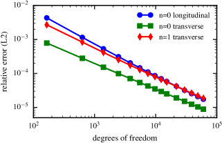
Figure 2: Convergence of numerical Fourier-FEM computations for analytical test cases. As expected the relative error decreases linearly with the number of degrees of freedom.

V Conclusion and Outlook

An approach for the numerical solution for the magnetostatic field on 3D domains with a symmetry direction has been described. In particular it is applicable to translationally symmetric and axisymmetric domains. Its validity has been demonstrated on model problems in cylindrical coordinatesSince each harmonic is computed separately, batch parallel computations are easily possible using the described method.

Even though arbitrary spatial variations of current density and boundary conditions can be treated, the approach is most efficient for symmetric current distributions reducing the number of non-zero harmonics. In axisymmetric domains this includes circular ($n=0$) or square-like shapes ($n=0,4,8,\dotsc$). Furthermore, smoother dependencies on the symmetry coordinate lead to a faster decay in the spectrum. A more severe limitation for engineering applications, apparent in the chosen model problems, is the restriction on the shape of regions with different permeability following the symmetry direction. To lift this requirement, coupling of different harmonics would have to be taken into account, thereby removing the original advantage of trivial parallelisability.

The method may be generalised further by considering an expansion in a different set of functions, e.g. Bessel functions for the expansion in cylindrical harmonics in the radial direction. For the treatment of time-dependent and time-harmonic eddy current or full electromagnetic wave problems the introduction of a an additional electromagnetic scalar potential will be required for the oscillatory harmonics if the gauge is fixed to eliminate one component of the vector potential.

References

- [1] J. G. V. Bladel, Electromagnetic Fields. John Wiley & Sons, Inc., 2007.
- [2] J.-M. Jin, The finite element method in electromagnetics. John Wiley & Sons, 2015.
- [3] C. Bernardi, M. Dauge, Y. Maday, and M. Azaiez, Spectral methods for axisymmetric domains. Gauthier-Villars Paris, 1999, vol. 3.
- [4] P. Lacoste, “Solution of Maxwell equation in axisymmetric geometry by Fourier series decompostion and by use of H(rot) conforming finite element,” Numer. Math., vol. 84, no. 4, pp. 577–609, 2000.
- [5] M. Oh, “de Rham complexes arising from Fourier finite element methods in axisymmetric domains,” Computers & Mathematics with Applications, vol. 70, no. 8, pp. 2063–2073, 2015.
- [6] M. F. Heyn, I. B. Ivanov, S. V. Kasilov, W. Kernbichler, I. Joseph, R. A. Moyer, and A. M. Runov, “Kinetic estimate of the shielding of resonant magnetic field perturbations by the plasma in DIII-D,” Nuclear Fusion, vol. 48, no. 2, p. 024005, 2008.
- [7] B. M. Dillon and J. P. Webb, “A comparison of formulations for the vector finite element analysis of waveguides,” IEEE Trans. Microw. Theory Tech., vol. 42, no. 2, pp. 308–316, 1994.
- [8] J. A. Schouten, Tensor analysis for physicists, 2nd ed. Dover, 1990.
- [9] E. J. Post, Formal structure of electromagnetics: general covariance and electromagnetics. Dover, 1997.
- [10] F. Gronwald, F. W. Hehl, and J. Nitsch, “Axiomatics of classical electrodynamics and its relation to gauge field theory,” Physics Notes, assembled by Dr. Carl E. Baum., no. 14, 2005. [Online]. Available: https://arxiv.org/pdf/physics/0506219
- [11] W. D. D’haeseleer, W. N. G. Hitchon, J. D. Callen, and J. L. Shohet, Flux coordinates and magnetic field structure. Springer Berlin Heidelberg, 1991.
- [12] T. Garavaglia and J. Gomatam, “The Schrödinger equation in helical coordinates,” Annals of Physics, vol. 89, no. 1, p. 1, 1975.
- [13] O. Bíró, “Edge element formulations of eddy current problems,” Computer Methods in Applied Mechanics and Engineering, vol. 169, no. 3-4, p. 391, 1999.
- [14] F. Brezzi and M. Fortin, Mixed and hybrid finite element methods. Springer Science & Business Media, 2012, vol. 15.
- [15] F. Hecht, “New development in FreeFem++,” J. Numer. Math., vol. 20, no. 3-4, pp. 251–265, 2012. [Online]. Available: https://freefem.org/