Reading between the lines:

Abstract

Aims. We use optical spectroscopy to investigate the disk, wind, and accretion during the 2008 Z CMa NW outburst.

Methods. Emission lines were used to constrain the locations, densities, and temperatures of the structures around the star.

Results. More than 1000 optical emission lines reveal accretion, a variable, multicomponent wind, and double-peaked lines of disk origin. The variable, non-axisymmetric, accretion-powered wind has slow ($\sim$0 km s^-1), intermediate ($\sim-$100 km s^-1), and fast ($\geq-$400 km s^-1) components. The fast components are of stellar origin and disappear in quiescence, while the slow component is less variable and could be related to a disk wind. The changes in the optical depth of the lines between outburst and quiescence reveal that increased accretion is responsible for the observed outburst. We derive an accretion rate of 10^-4 M_⊙/yr in outburst. The Fe I and weak Fe II lines arise from an irradiated, flared disk at $\sim$0.5-3 $\times$M_∗/16 M_⊙ au with asymmetric upper layers, revealing that the energy from the accretion burst is deposited at scales below 0.5 au. Some line profiles have redshifted asymmetries, but the system is unlikely to be sustained by magnetospheric accretion, especially in outburst. The accretion-related structures extend over several stellar radii and, like the wind, are likely to be non-axisymmetric. The stellar mass may be $\sim$6-8 M_⊙, lower than previously thought ($\sim$16 M_⊙).

Conclusions. Emission line analysis is found to be a powerful tool to study the innermost regions and accretion in stars within a very large range of effective temperatures. The density ranges in the disk and accretion structures are higher than in late-type stars, but the overall behavior, including the innermost disk emission and variable wind, is very similar for stars with different spectral types. Our work suggests a common outburst behavior for stars with spectral types ranging from M type to intermediate mass.

1 Introduction

Z CMa is a binary intermediate-mass star known for its strong photometric and spectroscopic variability (Covino et al., 1984; Shevchenko et al., 1999). The two components are separated by 0.1”, or about 100 au (Barth et al., 1994), for a distance of 1 kpc (Shevchenko et al., 1999; Kaltcheva & Hilditch, 2000). The SE companion is classified as a FU Orionis (FUor) object (Hartmann et al., 1989; Hessman et al., 1991), while the NW component is an embedded, variable intermediate-mass star, initially labeled as an infrared companion (Koresko et al., 1991). The NW component was detected later in the optical (Barth et al., 1994; Thiebaut et al., 1995) and classified as a 16 M_⊙, B0 III star based on its de-reddened photometric colors (van den Ancker et al., 2004), although its radius and luminosity are disputed (e.g., Monnier et al., 2005). A B0 spectral type would place the NW component of Z CMa among the earliest-type stars known to have a disk (e.g., see the reviews by Zinnecker & Yorke, 2007; Beltrán & de Wit, 2016) and to undergo variable accretion in a way not dissimilar to lower-mass objects, although disks similar to those of solar-type stars are also increasingly found around massive stars (e.g., Bik & Thi, 2004; Alonso-Albi et al., 2009; Kraus et al., 2010; Fedriani et al., 2020).

Z CMa has a complex light curve with anomalous variability (Shevchenko et al., 1999). Highly complex, short-timescale, aperiodic variations were confirmed by MOST (Microvariability and Oscillations of Stars; Siwak et al., 2013). Although historically the main variability was attributed to FUor, further observations, including polarization and scattered light, have suggested that the NW component is responsible for the most dramatic changes (Lamzin et al., 1998; Szeifert et al., 2010) and also dominates the polarization observed in the system (Fischer et al., 1998). The photometric evolution of Z CMa NW is uncertain since the first optical observations. Early works focussed on the FUor, but there are several reports of anomalous behavior that may be related to the NW component. Z CMa was always presented as an atypical FUor, in part for its long rising time (Hartmann et al., 1989; Hessman et al., 1991; Hartmann & Kenyon, 1996), but also because of its bumpy light curve. Several authors found the IR object to be brighter than expected in the optical since the 1990s, although Thiebaut et al. (1995) argued that this could be due to scattered light of the central object on the wall of a low-inclination bipolar cavity. The same conclusion of the NW component being optically brighter was reached by Barth et al. (1994) from observations obtained three years after Thiebaut et al. (1995). Subsequent interferometric observations revealed a $\sim$4 au dusty ring around Z CMa NW (Monnier et al., 2005) and a larger mid-infrared structure ($\sim$68 mas$\times$41 mas, $\sim$40-70 au) dominated by Z CMa NW but extended toward the FUor companion (Monnier et al., 2009). The FUor companion also has a ring that is similar in size (Millan-Gabet et al., 2006).

Table 1: Summary of spectroscopy observations.

MJD	Date	Instrument	Status
54813.114	2008-12-12	Sophie/OHP	Outburst
54820.047	2008-12-19	Sophie/OHP	Outburst
54839.43	2009-01-08	ESPaDOnS	Outburst
54840.446	2009-01-09	ESPaDOnS	Outburst
54841.438	2009-01-10	ESPaDOnS	Outburst
54843.363	2009-01-12	ESPaDOnS	Outburst
54844.356	2009-01-13	ESPaDOnS	Outburst
54845.501	2009-01-14	ESPaDOnS	Outburst
55121.170	2009-10-16	Sophie/OHP	Quiescence
55122.181	2009-10-18	Sophie/OHP	Quiescence
55123.182	2009-10-19	Sophie/OHP	Quiescence

The classification of the FUor object emphasized its double-peaked absorption lines, a telltale of strongly accreting sources (Hartmann & Kenyon, 1996). The spectra revealed a radial velocity $\sim$30 km s^-1, and double-peaked absorption lines consistent with a self-luminous disk 6 au in size and with maximum velocity $\sim$120 km s^-1 (Hartmann et al., 1989). In addition, Z CMa showed lines with strong P Cygni profiles (Hartmann et al., 1989; van den Ancker et al., 2004) that were enhanced during the episodes of anomalous, bumpy variability (Hessman et al., 1991). Covino et al. (1984) pointed out significant spectral variations since observations began in the 1920s, and several authors have suggested that the origin of the strong line emission lies in the NW component (Garcia et al., 1999; Benisty et al., 2010; Szeifert et al., 2010; Bonnefoy et al., 2017).

There is little information on the accretion mechanisms and accretion evolution in intermediate-mass stars. Unlike T Tauri stars, Herbig Be (HBe) stars are not expected to have magnetospheric accretion as their magnetic fields are too weak (Alecian et al., 2013) as well as very small magnetospheres (Cauley & Johns-Krull, 2015). This would lead to a different accretion mechanism compared to solar-type stars (Cauley & Johns-Krull, 2016), such as a boundary layer (Popham et al., 1993; Vink et al., 2002; Eisner et al., 2004; Mendigutía et al., 2011; Wichittanakom et al., 2020), a hot inner disk scenario (e.g., Fairlamb et al., 2015; Mendigutía et al., 2015), or non-axisymmetric radial flows (Mendigutía et al., 2017). Therefore, exploring the small-scale accretion structures is especially important in objects such as Z CMa NW.

A new outburst started in January 2008 (Grankin & Artemenko, 2009), ending in October 2009. High spatial resolution observations confirmed that the intermediate-mass Z CMa NW was responsible for the increased brightness, and also resolved the near-infrared (near-IR) spectra of both components, revealing the expected characteristic lines of FUor objects for the SE companion, and a large number of emission lines reminiscent of EXor variables for Z CMa NW (Bonnefoy et al., 2017). An enhanced bipolar wind with velocities up to 700 km s^-1 was also detected during the outburst (Benisty et al., 2010; Szeifert et al., 2010), which is a further sign that variability episodes are related to increased accretion.

In this paper, we present the spectroscopic analysis of the 2008-2009 outburst and return to quiescence of Z CMa NW, exploring the physical structure and properties in the wind and the innermost disk with the aim of understanding accretion in high-mass stars. Observations, data reduction, and emission line classification are presented in Section 2. The analysis of the emission lines is presented in Section 3, while the implications for the outbursts of massive versus low-mass stars are discussed in Section 4. Our results are summarized in Section 5.

2 Observations and data reduction

2.1 Spectroscopic data

Two series of spectra were obtained for Z CMa at the Observatoire de Haute-Provence (OHP) using the SOPHIE spectrograph (Perruchot et al., 2008). The first set of two spectra was obtained on 2008 December 12 and 19 during the outburst. An additional set of three spectra was obtained with the same setup from 2009 October 16 to 19 as the system had returned to quiescence. OHP/SOPHIE spectra are automatically reduced online at the telescope to provide a continuum normalized 1D spectrum ranging from 382 to 693 nm at a spectral resolution of 39,000. With an integration time of 1 hour, and depending on weather conditions, the spectra have a signal-to-noise ratio (S/N) ranging from 40 to 150 at 600 nm. Another series of spectra were obtained with the Echelle SpectroPolarimetric Device for the Observation of Stars (ESPaDOnS; Donati, 2003) in spectroscopic mode at the Canada-France-Hawaii Telescope (CFHT) from 2008 January 8 to 14 as the system was reaching the peak of the outburst. A total of six spectra were obtained over seven nights, covering from 370 nm to 1000 nm at a spectral resolution of 65,000. An exposure time of 4800 s yielded a S/N of 500-600 at 600 nm. Spectra were reduced with the Libre-Esprit software (Donati et al., 1997) to provide continuum normalized 1D spectra. Table 1 summarizes the available spectroscopic data.

Our data are not spatially resolved, so the spectra contain emission from both Z CMa NW and from the FUor companion. We assume that the FUor contribution can be neglected during outburst because the luminosity is at least 8 times higher during outburst as in quiescence, the FUor outburst seems to have ended (or substantially weakened) after 1995 (see Appendix A), and the wind component has been estimated to be at least 20 times stronger for Z CMa NW in outburst as for the FUor (Antoniucci et al., 2016). The quiescence spectra do not reveal any features typical of a FUor. Even though there is a larger relative contribution from the FUor companion, the spectra resemble those of a typical, strongly accreting intermediate-mass star. The FUor features such as double-peaked absorption components that were present before (e.g., Hartmann et al., 1989; Hartmann & Kenyon, 1996) are no longer observed, indicating the evolution of the FUor outburst in the last $\sim$20 years. We thus suspect that the quiescence data may also be dominated by Z CMa NW, although a significant contribution from the companion cannot be excluded.

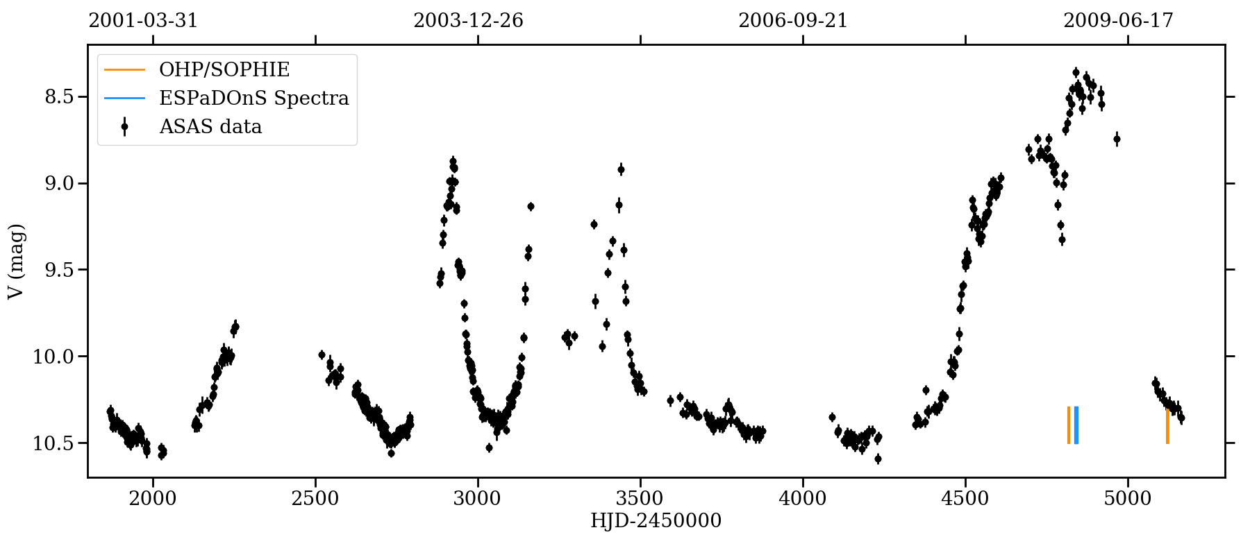
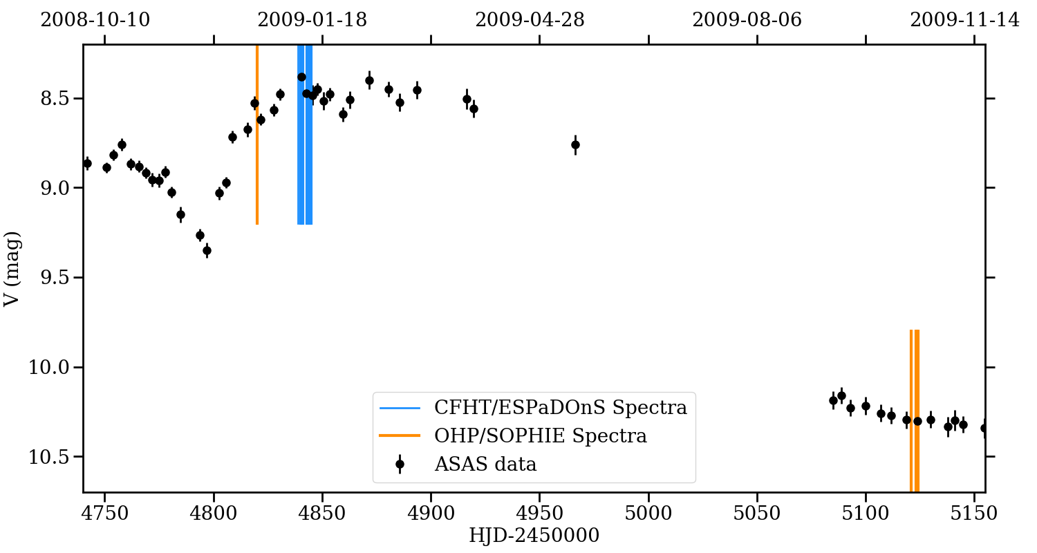
Figure 1: Full light curve (left) from ASAS and zoom around the times of the spectroscopic observations (right). The times at which the spectra were taken are indicated as blue for outburst spectra and orange for quiescence spectra. A complete light curve is given in Appendix A, Figure 16.

2.2 Photometric observations

Z CMa was observed by the All Sky Automated Survey (ASAS; Pojmanksy, 2003) between December 2000 and December 2009 in the V filter. The photometry is calculated using five different apertures. We chose the smallest (2 pix, where the native pixel is 15”) to minimize the amount of nebular emission included, although the differences between apertures are negligible, especially considering the variability range. Only the quality A data are used, containing 637 photometric data points spread over nine years (Figure 1). The ASAS data include the full outburst, rising from quiescence levels by more than two magnitudes and coming back to quiescence, and offer a good baseline to explore the status of the object at the time of the spectroscopic observations. The ASAS data also reveal that, although the 2009 outburst is significantly longer and very bright, the source has suffered several bursts, rising to nearly the same magnitude for shorter times, since their records started.

The historical data from the American Association of Variable Stars Observers (AAVSO; see Appendix A) show that the smooth FUor outburst profile is punctured by brief bursts (similar to the bumps cited by Hessman et al., 1991) since the early 1980s. The overall shape of the light curve suggests that the NW component has become increasingly active and likely brighter and less extincted in the last $\sim$40 years. The FUor outburst had faded substantially by 1995. More recent AAVSO observations show that the bumpy behavior recorded by ASAS continues until the present day (see Figure 16), so that the outbursts described in this work are recurrent.

Analysis of the ASAS data does not reveal any significant periodic signature on short (days–months) or long (months–years) timescales. A low-significance 249 d quasi-period can be derived from the whole V data (ASAS plus the AAVSO, see Appendix A), suggesting that outbursts happen roughly every 249 days. Such a period is similar to that of a body in Keplerian rotation at a distance 2.0$\times$(M_∗/16 M${}_{\odot})^{1/3}$ au. Regular perturbations of the disk by companions may trigger outbursts (Lodato & Clarke, 2004), although the results have low significance and need follow up for confirmation. The ASAS data also show a brief dip or occultation event that happened just before the first spectrum was acquired. Although the dip was not completely over at the time of the first observation, we do not find any significant spectroscopic signature linked to this event.

2.3 Emission line classification

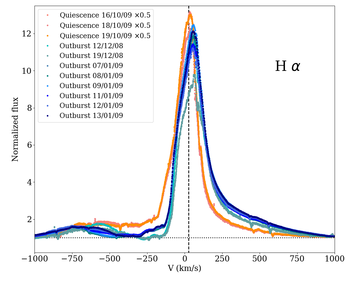
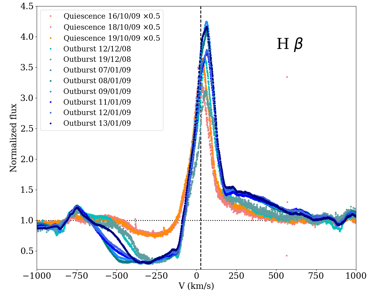
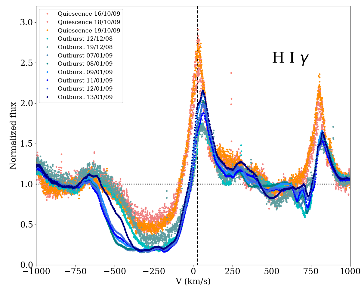
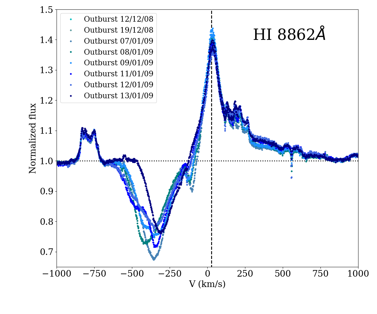
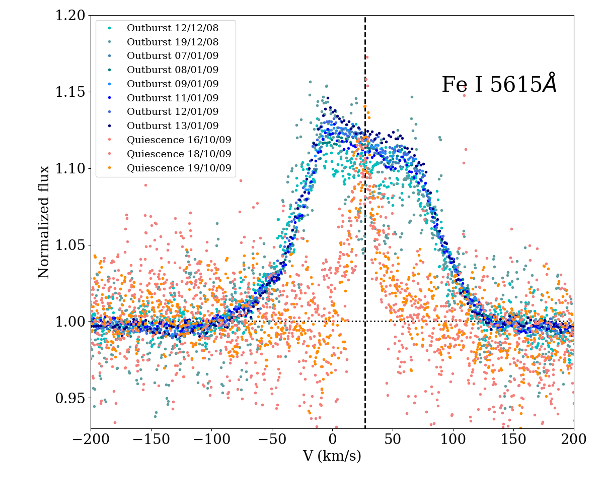
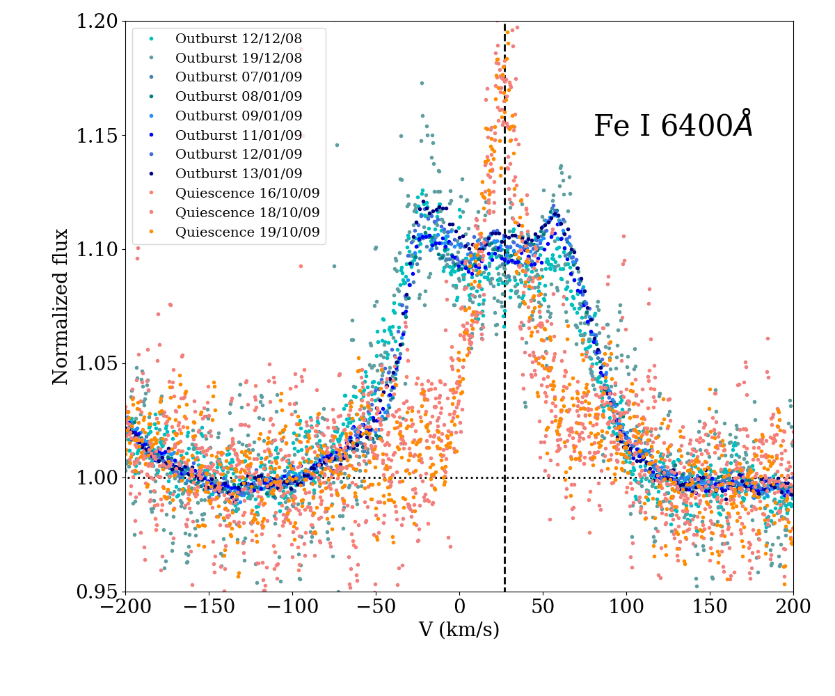
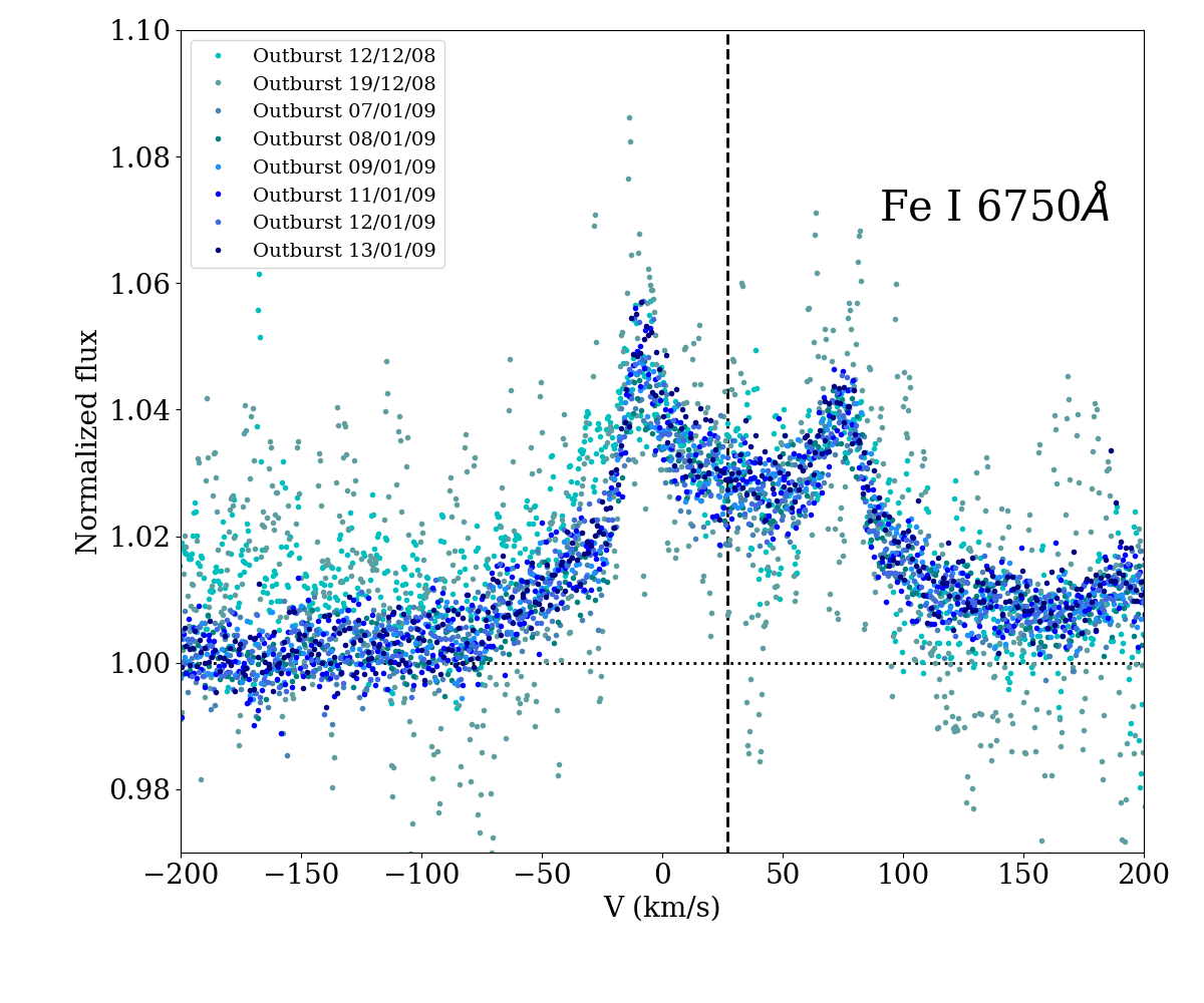
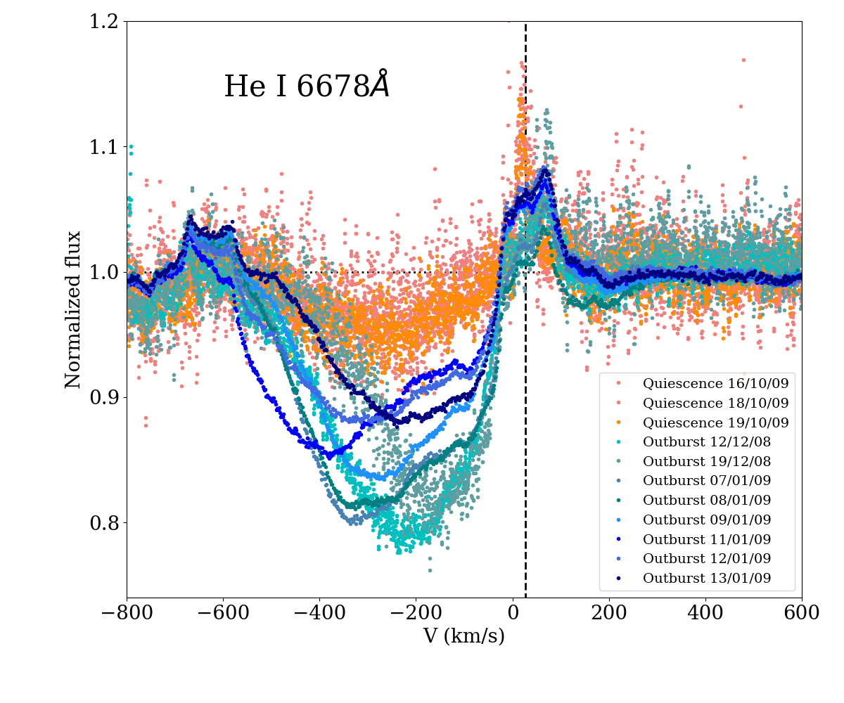
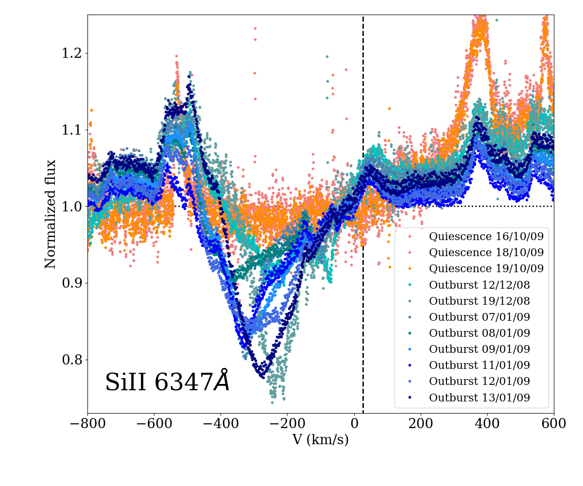
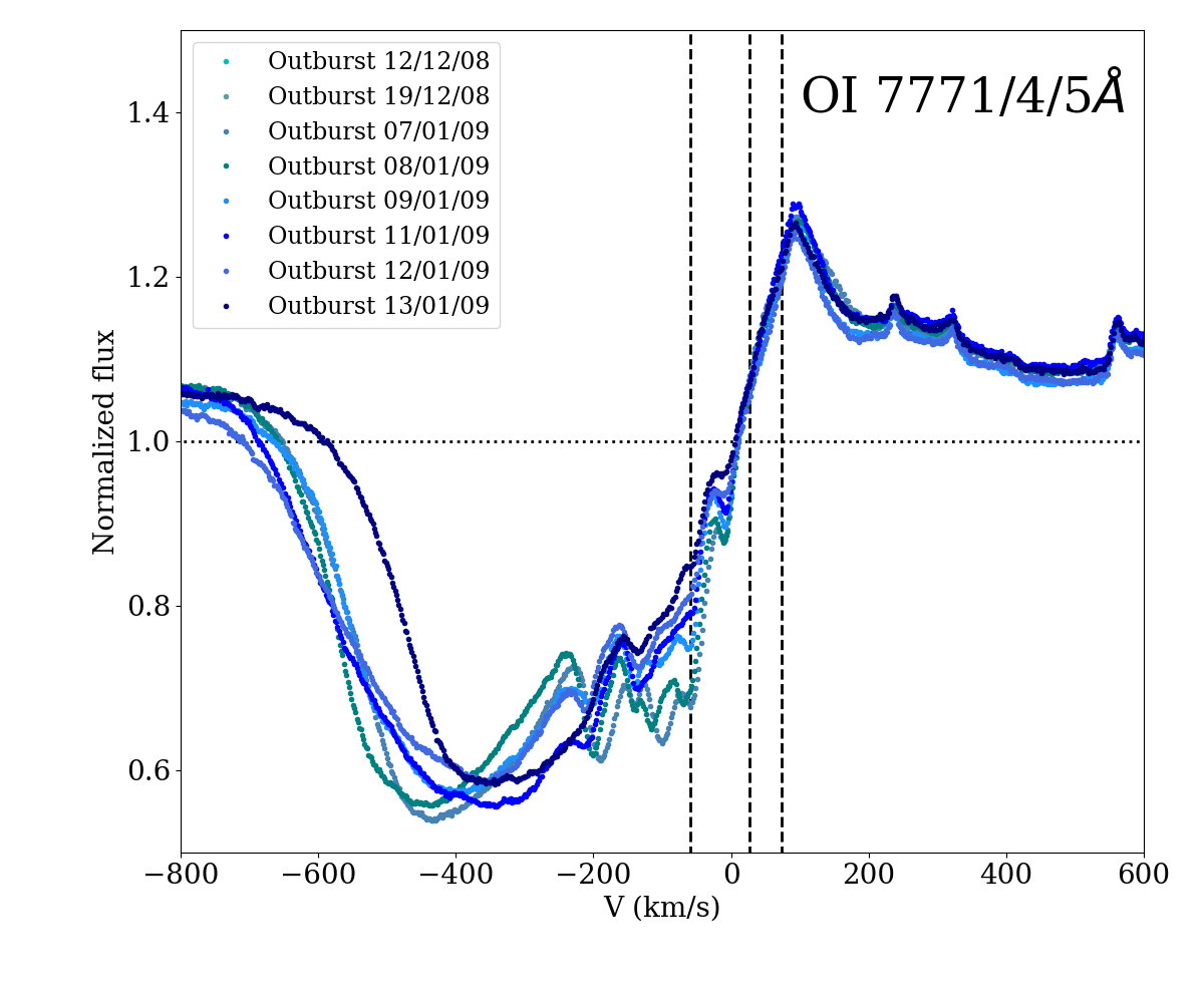
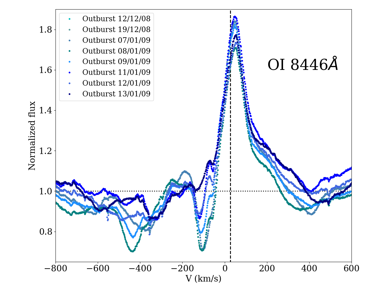
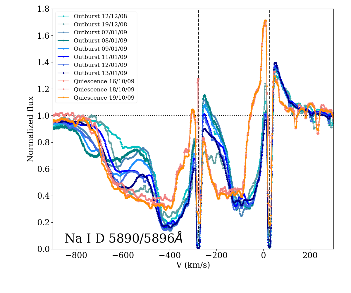
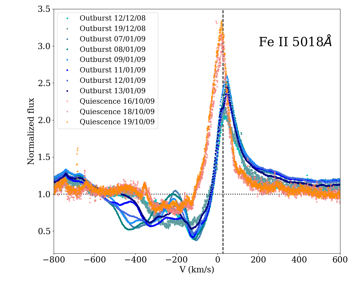
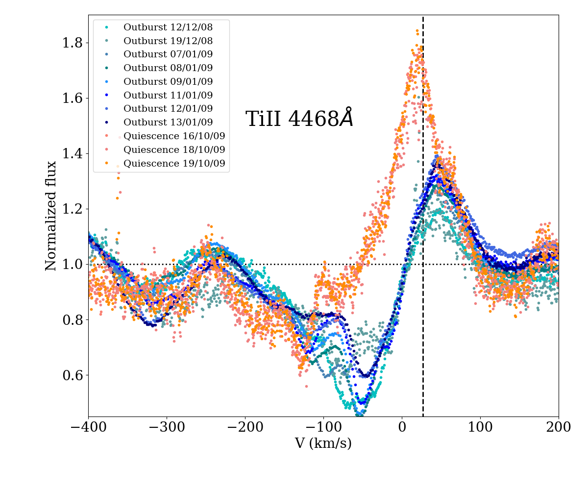
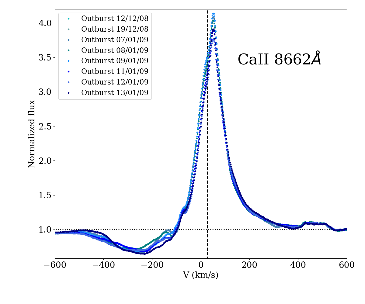
Figure 2: Examples of lines observed for Z CMa. The lines are normalized to the local continuum. In this and the following figures, the quiescence data are plotted in various shades of orange, while the outburst spectra are shown in blue. The dashed line shows the radial velocity of the system (27 km s^-1) and the dotted line indicates the continuum level. First row: Some H Balmer lines and an IR H line. The quiescence spectra of H$\alpha$ and H$\beta$ are scaled by $\times$0.5 for better display. Second row: Some of the Fe I lines with disk-like profiles and a K I resonance line. Third and fourth row: Some lines with various types of P Cygni profiles. The quiescence spectra do not cover the range beyond 6940 Å.

The emission lines were visually selected and classified using the NIST database (Ralchenko et al., 2010; Kramida et al., 2018) and the list of lines observed in Z CMa and other outbursting objects (van den Ancker et al., 2004; Sicilia-Aguilar et al., 2012, 2015, 2017). The narrow neutral metallic emission lines in quiescence reveal a radial velocity $\sim$27$\pm$3 km s^-1, which is consistent with previous estimates ($\sim$30 km s^-1; Hartmann et al., 1989). This radial velocity was used to revise the classification of the remaining emission lines, in particular, those that were weak or not observed in other young stars. In total, we estimated more than 1000 emission lines in the optical outburst spectra, but because of low S/N and blends, we only resolved 497 of these, among which 26 lines cannot be identified in the literature. The complete line list is presented in Appendix B (Table LABEL:alllines-table). The table contains all identified lines plus blends, together with excitation potentials, transition probabilities, profile types, strength, and whether they have been observed in outburst and/or quiescence.

The lines include typical H, He, and Ca II emission plus a large number of Fe I, Fe II, Ti I, Ti II, Si II, and other metallic lines commonly found in young stars (Joy, 1945; Hamann & Persson, 1992). Nearly all lines correspond to permitted transitions and the only forbidden lines that can be clearly identified are the [O I] lines at $\lambda\lambda$6300, 6363Å and the [S II] lines at $\lambda\lambda$6717, 6731Å. Many of these are common to both quiescence and outburst, but their profiles are different. Several examples of lines with various profiles are shown in Figure 2. Although most of the lines are broad in both quiescence and outburst, the outburst lines are significantly broader; some such as H$\alpha$ have line wings up to $\pm$1000 km s^-1. A P Cygni profile is most common among the strong, high-energy lines, such as H and Fe II, in both outburst and quiescence; 89 lines have this kind of profile. Very high energy lines, such as He I and Si II, have extreme P Cygni profiles in outburst, which are entirely dominated by blueshifted absorption and with a very small emission component (see Figure 2), being thus the only lines that show the typical profiles of FUor objects. No such lines are observed in quiescence, so they are likely related to the outbursting Z CMa NW and not to the FUor. The blueshifted absorptions become much weaker (or disappear completely, especially in the most energetic lines) in the quiescence spectra. This suggests a powerful hot wind developing during outburst that is likely related to the increased accretion episode. Most of the outburst blueshifted absorption features have several components and show a very high degree of variability, as we discuss in Section 3.2.

We detected many low-energy, neutral metallic lines in emission during both quiescence and outburst, especially Fe I. In quiescence, most of the Fe I, Na I, and Ni I lines are narrow (FWHM $<$30 km s^-1) or absent, while in outburst, 91 of these lines show a box-like or double-peaked profile as expected for Keplerian disk emission (Horne & Marsh, 1986) and similar to the disk emission profiles observed in HAeBe stars in CO (e.g., Hein Bertelsen et al., 2016). The double-peaked profiles are very similar to those observed by Hartmann et al. (1989) in FUor objects, but they are in emission instead of in absorption. Although viscous dissipation often dominates disk heating in strongly accreting systems (producing a disk that is hotter in the midplane than in the surface; Hartmann et al., 1989), this is a signature of a temperature inversion in the Z CMa NW disk, which remains hotter in its upper layers as seen in irradiated disks (Calvet et al., 1992). Interferometry and polarimetry have also revealed structures that are consistent with disks in some HBe stars (Eisner et al., 2004; Ababakr et al., 2017), which could be similar to what we trace in the neutral metallic lines. There are differences in the disk-like profiles, considering line strength (or transition probability) and some asymmetries in the blue- versus redshifted parts. The former is expected since lines with various strengths saturate at different heights over the disk and stronger lines can be produced over larger, less well-defined regions (and may thus include other components, including low-velocity ones) compared to weaker lines, resulting in box-like rather than double-peak profiles (Ferguson, 1997). The latter could be related to asymmetries in the disk and/or wind- or accretion-related absorption components, which is discussed in detail in Sections 3.4 and 3.5.

Redshifted absorptions are typically a clear indication of infall in the spectra of young stars. We did not observe clear redshifted absorptions in the Z CMa spectra, although there are several lines with redshifted asymmetries that could be consistent with weak absorption components at various velocities. Redshifted absorption asymmetries were observed at $\sim$200 km s^-1 in the higher Balmer lines, IR H lines, the O I line at 8446Å  and the Ca II IR triplet (Figure 2). As we discuss in Section 3.6, Fe I lines also have weak redshifted asymmetries in outburst and quiescence that could be related to absorption components, although the velocities are significantly lower.

Regarding forbidden line emission, the [O I] line is the most evident because of its strength and lack of blends with other features. The [O I] lines have two components with typical shock profiles (Figure 3): one component slightly blueshifted with respect to the source velocity and a second, high-velocity component at $\sim-$420 km s^-1. The high-velocity component is consistent with the high-velocity peak of the jet identified by Whelan et al. (2010), who also detected the SE source jet at velocities $-$300 to $-$100 km s^-1 (not evident in our spectra). [S II] emission at 6731 and 6717Å is also observed. Its high-velocity component at -400 km s^-1 is detected in quiescence, but it is negligible in outburst, which could be a contrast effect combined with blending with other broad lines in the outburst spectrum. Additional [N II] emission and some [Fe II] lines may be also present, but because they are heavily blended with other lines (see Table LABEL:alllines-table), it is hard to confirm their presence and to reveal any details about their velocity components.

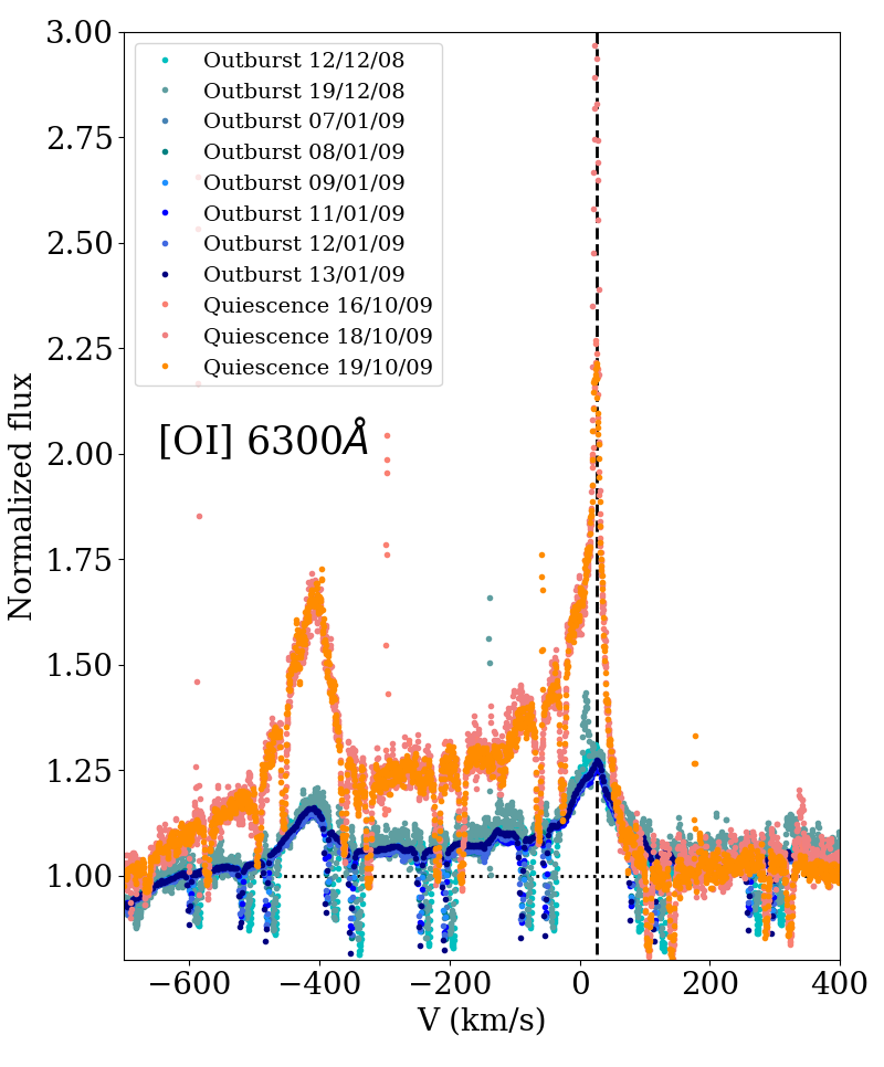
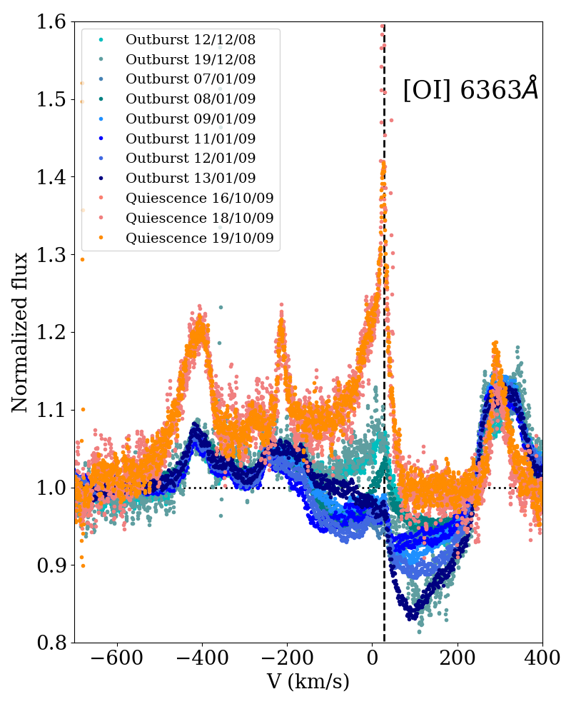
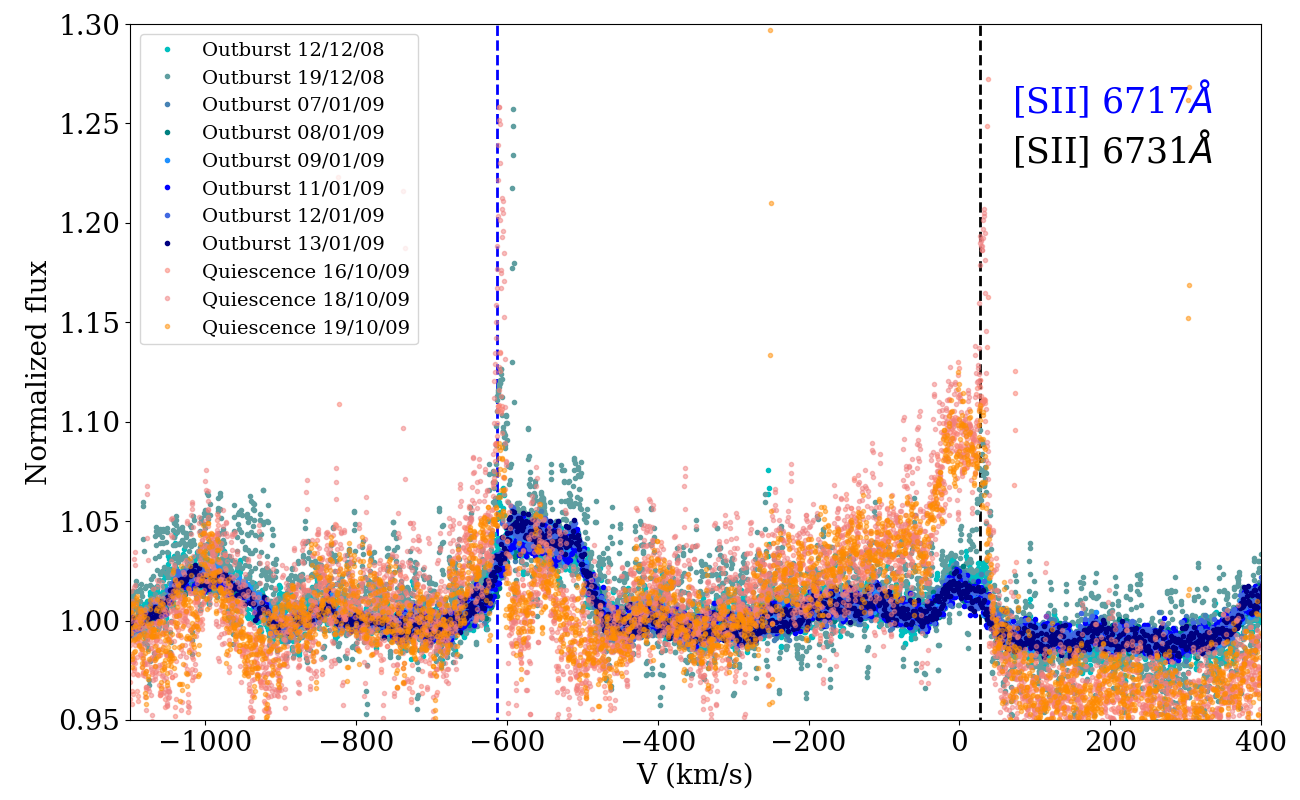
Figure 3: Upper: Forbidden [O I] emission. Lower: Forbidden [S II] emission. The dotted lines indicate the the continuum level, and the dashed lines represent the radial velocity of 27 km s^-1. The data from the outburst are plotted in various shades of blue, while the quiescence data are shown in orange. The extra lines observed in the 6363Å spectrum correspond to unrelated Fe I and Fe II lines, and the strong absorption is due to Fe II 6369Å. The narrow absorption lines are telluric.

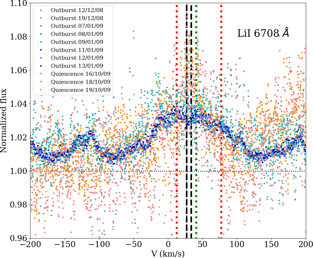
Figure 4: Zoom around the Li I 6708Å line. The dotted black line indicates the continuum level, the dashed black lines indicate the Li I transitions (6707.76 and 6707.91Å), the vertical red dotted lines indicate the Fe I 6707.43Å and Fe II 6708.88Å lines, and the green dotted line indicates the V I line at 6708.07Å; all of these are shifted to match a radial velocity of 27 km s^-1. The emission feature in quiescence is likely due to the high-velocity component of [S II].

The Li I resonance line, which is characteristic of young T Tauri stars (White & Basri, 2003), is also detected (Figure 4), albeit mostly in emission, as observed for V1118 Ori in its 2005 outburst (Herbig, 2008). In outburst, the line has a profile that is very similar to that of EX Lupi in outburst with broad line wings in emission and a shallow absorption at the stellar rest velocity (Sicilia-Aguilar et al., 2012); this could suggest a similar origin. It is nevertheless very hard to produce Li I emission under normal conditions and abundances (e.g., Shore & De Gennaro Aquino, 2020), so we explored other possibilities. The profile is clearly different from disk- or box-like profiles, which have distinct peaks or, for box-like lines, a central peak instead of a central absorption. As in the case of EX Lupi, Li I is the only line with this type of profile. There is potential contamination by nearby Fe I and Fe II lines and by the high-velocity component of the [S II] line at 6717Å, which is likely the cause of the emission feature observed in quiescence, although the wavelength of the weak absorption feature is more consistent with Li I. It is unlikely that [S II] is responsible for the feature observed at 6708Å during outburst because the high-velocity component of the 6731Å [S II] line is negligible. The Fe II line is clearly more energetic than the typical Fe II emission observed, and thus unlikely to contribute. The Fe I line is only slightly more energetic than observed Fe I emission lines, so a contribution is hard to rule out, although it would be blueshifted. In addition, a V I line could be also present at 6708.07Å and has similar energetics to the V I line observed at 6643.786Å, which has a disk-like profile in outburst and an emission profile in quiescence. Nevertheless, the lack of consistency between the profiles of the tentative V I identifications makes the association uncertain. Li I absorption is usually not seen in stars earlier than F0 (Zappala, 1972), which could hint at an origin in very hot and dense circumstellar material or inner hot disk atmosphere for the small absorption feature.

Finally, a handful of absorption lines are observed, mostly in quiescence, but some of these lines are also observed in outburst (e.g., 5781, 5798 6614Å), which are likely diffuse interstellar bands (DIBs; Herbig, 1995; Hobbs et al., 2008). There is no clear identification of photospheric absorption lines in outburst nor quiescence.

3 Analysis

In this section, we constrain the properties of the various components of the star-disk system using the emission and absorption lines. First, we revise the stellar parameters and accretion in Section 3.1, followed by a discussion of the wind components in Section 3.2. Then, we use several methods to extract information about the physical conditions and velocities from the observed emission lines. The details of the methods are given in Appendix C. There are many uncertainties in the structure of a complex object such as Z CMa NW, so we use various techniques that work under different assumptions. These include Saha’s equation, which assumes local thermodynamic equilibrium (LTE), and ratios from lines from the same upper level, which do not depend on ionization equilibrium (Beristain et al., 1998). We finally use velocity brightness decomposition for disk-like profiles (Acke & van den Ancker, 2006) to introduce further constraints derived from the line profile on the velocity, temperature, and density structure of the system, as well as to reveal where the observations depart from the simplified models. Blended lines and those that may belong to several species and/or transitions are excluded from the analysis. In addition, non-LTE effects and line pumping may affect line ratios; for instance, due to strong UV emission lines directly feeding the upper level of a line. Lacking UV data, but knowing that lines in the UV, as in the optical, may be very broad, we used the exhaustive line list from Herczeg et al. (2005) for the young star RU Lupi to exclude any line that could be pumped by UV lines with $\pm$1000 km s^-1 wings.

3.1 Constraining the stellar properties and accretion

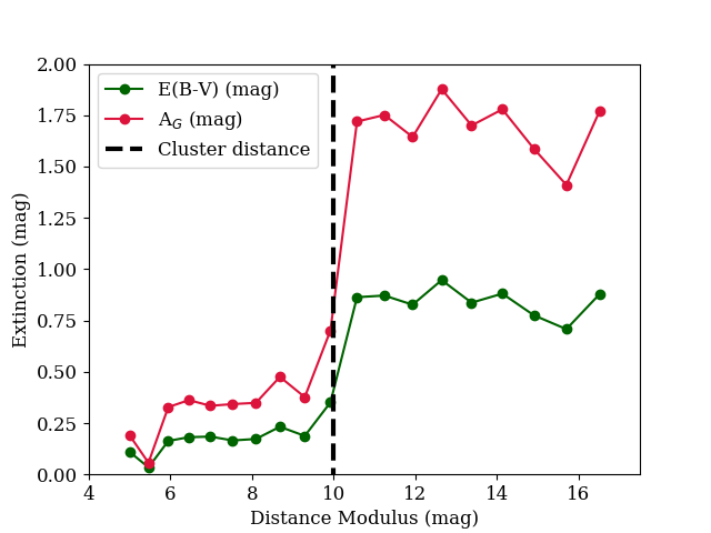
Figure 5: Extinction in the Gaia G band and Gaia BP-RP around a 0.2 degree radius field toward Z CMa. The rise of extinction is fully consistent with the location of the Z CMa cloud at 1 kpc.

Because of the disagreements regarding the spectral type and quiescence luminosity of the star (van den Ancker et al., 2004; Monnier et al., 2005), our first step was to revise these assumptions. First, we used Gaia DR2 data to revise the distance. Z CMa itself is not a reliable Gaia source because it is too bright, is a binary, and is surrounded by nebulosity. Nevertheless, a rise in extinction at a certain distance can be used to identify the location of its cloud (Green et al., 2015; Sicilia-Aguilar et al., 2017). Examining the Gaia DR2 stellar extinction for stars 0.2 degrees around Z CMa reveals a clear rise around 1 kpc (Figure 5), confirming the previously assumed distance to the Z CMa cloud, and thus the stellar luminosity. For a quiescence luminosity of 2400 L_⊙ (Thiebaut et al., 1995) and assuming that the system has an age in the 0.3-3 Myr range, the CMD 3.3 stellar evolutionary tracks (Bressan et al., 2012; Marigo et al., 2017; Pastorelli et al., 2019) suggest a mass between 6-8 M_⊙. The temperature would be consistent with a B-type star (16000-22000 K), albeit later than B0. The star could be colder ($\gtrapprox$10000 K) but similarly massive if it is younger than 0.3 Myr. Assuming that half of the observed luminosity in quiescence is due to accretion, we still get a mass between 6 M_⊙ and 8 M_⊙ and a temperature between 13000 K and 20000 K (for ages 0.3-2 Myr) or 8000 K and 13000 K (for ages younger than 0.3 Myr). So while the object is definitely an intermediate-mass star, the mass is likely lower and the spectral type is uncertain.

We thus adopted the quiescence luminosity of L_∗=2400 L_⊙ and give all results as a function of stellar mass. An effective temperature of 29200 K (for a B0 star) results in a stellar radius of about 1.93 R_⊙ in quiescence, but the radius would be larger if T_eff is lower, especially if the star is very young. During outburst, the luminosity increased by a factor of 8. Assuming a blackbody-like scenario, the effective temperature for this increased luminosity could reach 49100 K if the emission originated from the star. Nevertheless, we expect a range of temperatures for the star and innermost disk and accretion structures. Despite all these uncertainties, if we assume that the extra energy due to accretion during outburst is dissipated in the innermost regions (star and innermost disk), the temperature of the regions outside this area depends on the total luminosity rather than on the actual temperature and radius of the star or the size of the emitting region. The temperature required for silicate dust sublimation ($\sim$1500 K) is reached at $\sim$3.4 au during quiescence (consistent with the dusty ring at 4 au resolved by Monnier et al., 2005) and at $\sim$9.6 au in outburst. These distances are lower limits to the inner dusty rim in the disk, its radius could be larger if there is in situ disk heating. Large amount of silicates may have been vaporized in outburst. The temperatures at 1 au are $\sim$2800 K in quiescence and $\sim$4700 K in outburst. Orbital velocities are 120$\times(M_{*}/16M_{\odot})^{1/2}$ km s^-1 at 1 au, and 38$\times(M_{*}/16M_{\odot})^{1/2}$ km s^-1 at the outburst dust sublimation radius (9.6 au).

The accretion rate (Ṁ) can be estimated from the increase in luminosity, as the luminosity in outburst is significantly higher than the quiescence luminosity of the object. For T Tauri stars with magnetospheric accretion, the accretion luminosity is

$$L_{acc}=\frac{GM_{*}\dot{M}}{R_{*}}\bigg{(}1-\frac{R_{*}}{R_{in}}\bigg{)},$$ (1)

where M_∗ and R_∗ are the stellar mass and radius, G is the gravitational constant, and R_in is the radius from which the material is accreted (usually, the magnetospheric or corotation radius in T Tauri stars; e.g., Gullbring et al., 1998; Sicilia-Aguilar et al., 2010; Fairlamb et al., 2015). We assume that the infall factor $(1-R_{*}/R_{in})$ is about 0.5, which can be attained from material infalling from a minimum distance of 2 stellar radii and is also equivalent to the result for a boundary layer (Bertout et al., 1988). We obtain Ṁ$\sim$10^-4 $\times(16M_{\odot}/M_{*})$ M_⊙/yr, which is similar to the accretion rates of FUors (Hartmann & Kenyon, 1996). In general, B stars are fast rotators (Abt et al., 2002; Müller et al., 2011), which results in small, if any, magnetospheres (Tambovtseva et al., 2016). A magnetosphere extending to several times the stellar radius would result in a lower accretion rate, while detailed boundary layer fits to B stars tend to produce higher accretion estimates (Wichittanakom et al., 2020).

The feasibility of free-falling material feeding accretion can be also estimated looking at the free-fall velocity, $v_{ff}$,

$$v_{ff}=\bigg{(}\frac{2GM_{*}}{R_{*}}\bigg{)}^{1/2}\bigg{(}1-\frac{R_{*}}{R_{in}}\bigg{)}^{1/2}.$$ (2)

For Z CMa and an infall factor of 0.5, we obtain a free-fall velocity $\sim$1200$\times(M_{*}/16M_{\odot})^{1/2}$ km s^-1. This is similar to the velocities observed in the H$\alpha$ line wings (up to $\sim$ 1000 km s^-1), but H$\alpha$ can be strongly affected by Stark broadening. The strongest metallic lines have maximum velocities of the range of 500-600 km s^-1 and any redshifted absorption features appear at lower velocities (see Section 2.3). Therefore, whether velocities can be explained by free-fall needs further discussion after other possibilities have been considered (Section 4).

Some initial constraints on the density can be derived from the estimated accretion rate. Assuming that accreted material moves in at a typical velocity $v$ over one or more accretion channels that cover a fraction $f$ of the stellar surface, we can write

$$\dot{M}=4\pi R_{*}^{2}fv\rho=4\pi R_{*}^{2}fv\mu m_{H}n,$$ (3)

where $\rho$ is the density of the accreting material, which can be written in terms of the mean atomic weight ($\mu$=1.36 is a typical value), the mass of the hydrogen atom ($m_{H}$), and the number density ($n$; e.g., Sicilia-Aguilar et al., 2012). Taking a typical velocity $v$=500 km s^-1, we obtain a density $n\sim$1.6e14$/f$ cm^-3. For any small value of $f$, these densities are about two orders of magnitude larger than observed in outbursting T Tauri stars. Nevertheless, if the material is brought onto the star via an extended structure involving part of the innermost disk, we could have $f>1$ and lower densities, as found, for instance, for ASASSN-13db (Sicilia-Aguilar et al., 2017, but note that ASASSN-13db has magnetospheric accretion).

Temperature estimates also suggest that the energy is deposited over a region larger than the stellar surface. If the accretion luminosity was released in a stellar spot at the stellar surface, the temperature of the spot could be unphysical, reaching (47e3/$\sqrt{f}$) K, where $f$ is the fraction of the stellar surface covered by the spot. Assuming a boundary layer scenario, the boundary layer temperature $T_{BL}$ can be written as

$$T_{BL}=\bigg{(}\frac{L_{acc}}{4\pi R_{*}\delta\sigma}\bigg{)}^{1/4},$$ (4)

where $\sigma$ is Stefan’s constant, $\delta$ is the scale of the boundary layer, and the rest of symbols retain their previous meanings (Popham et al., 1993; Blondel & Djie, 2006; Mendigutía, 2020). The value of $\delta$ is calculated as

$$\delta=\delta_{0}R_{*}\bigg{[}1-\bigg{(}\frac{\Omega_{*}}{\Omega_{K}}\bigg{)}^{2}\bigg{]}^{-1/3},$$ (5)

where $\delta_{0}$ is a scale parameter, with typical values between 0.01-0.5 (Popham et al., 1993; Blondel & Djie, 2006); $\Omega_{*}$ is the angular velocity of the star; and $\Omega_{K}$ is the Keplerian angular velocity. For a rotation rate of 25% of the breakup velocity (typical for B stars; Abt et al., 2002), $\delta_{0}$=0.5 would still result in T${}_{BL}\sim$56,000 K, therefore the requirement of a structure that extends over several stellar radii remains. This is also consistent with the very extended boundary layers, often hard to distinguish from the disk, expected in objects with very high accretion rates (Popham et al., 1993).

3.2 Wind variability in outburst and quiescence

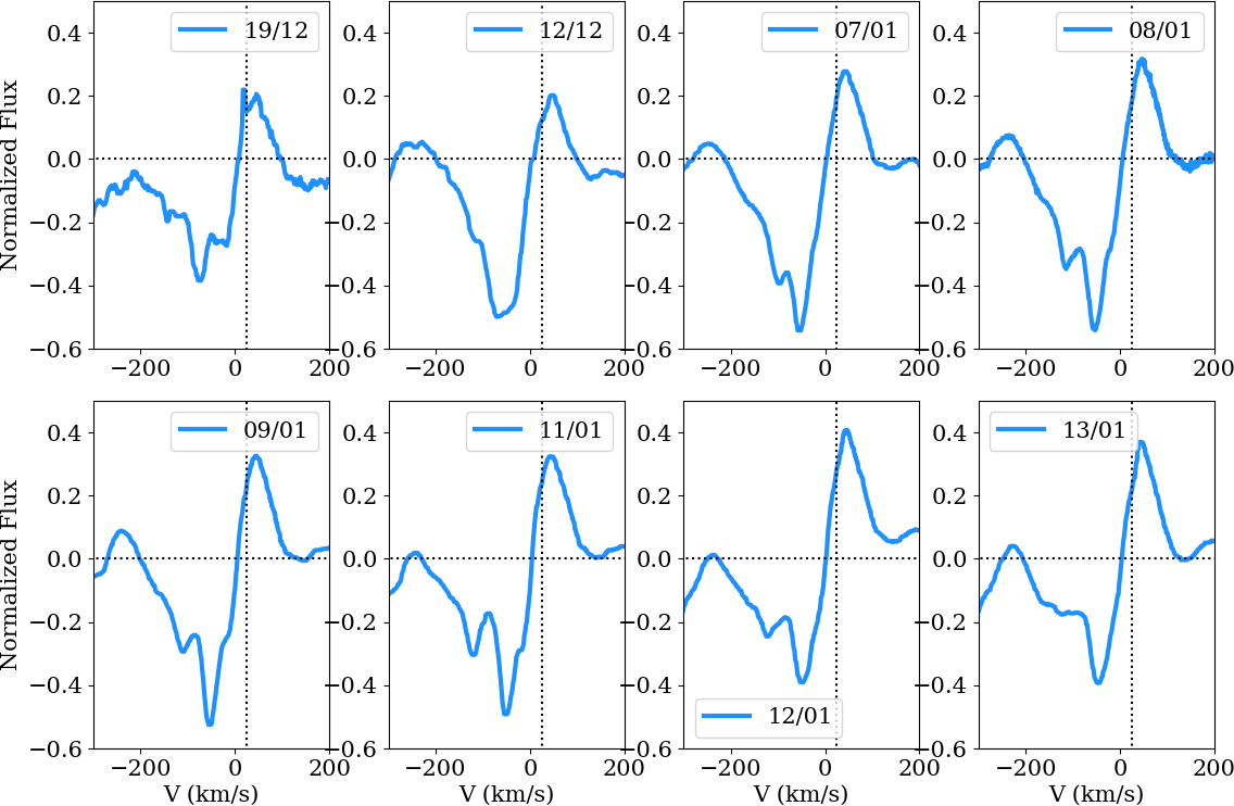
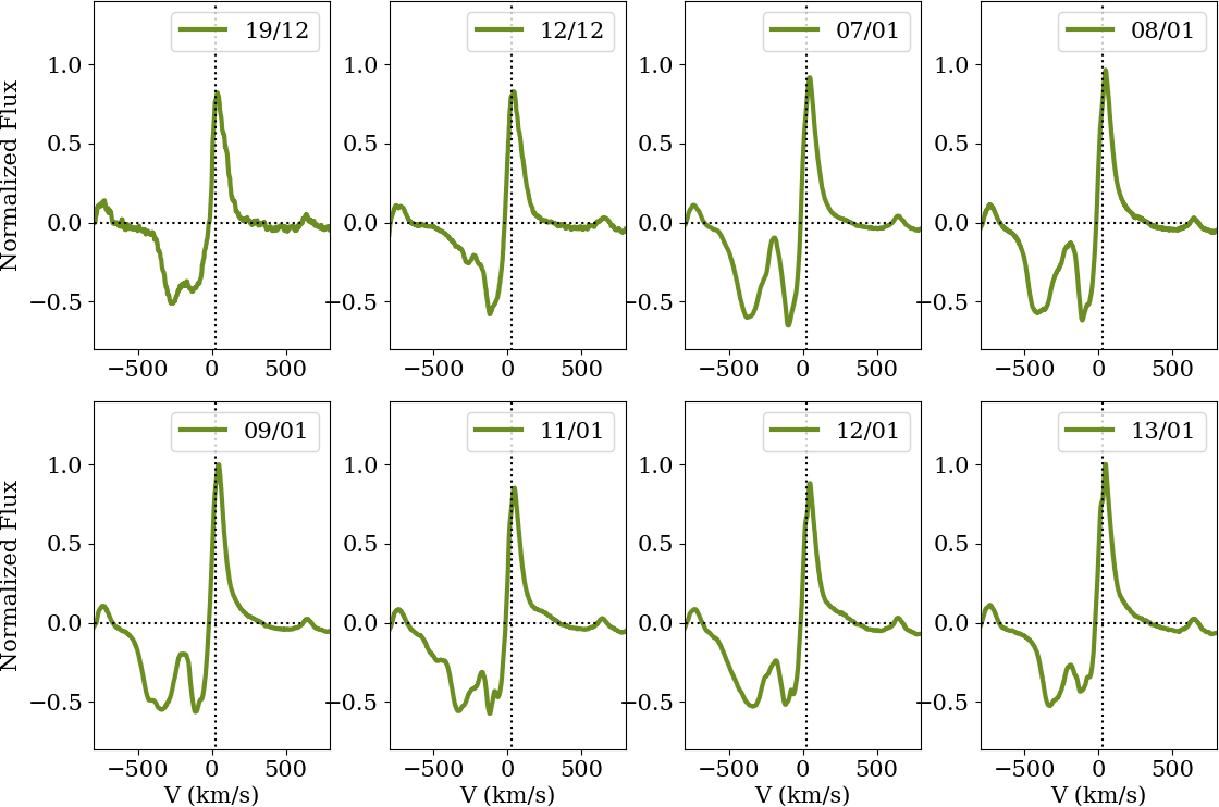
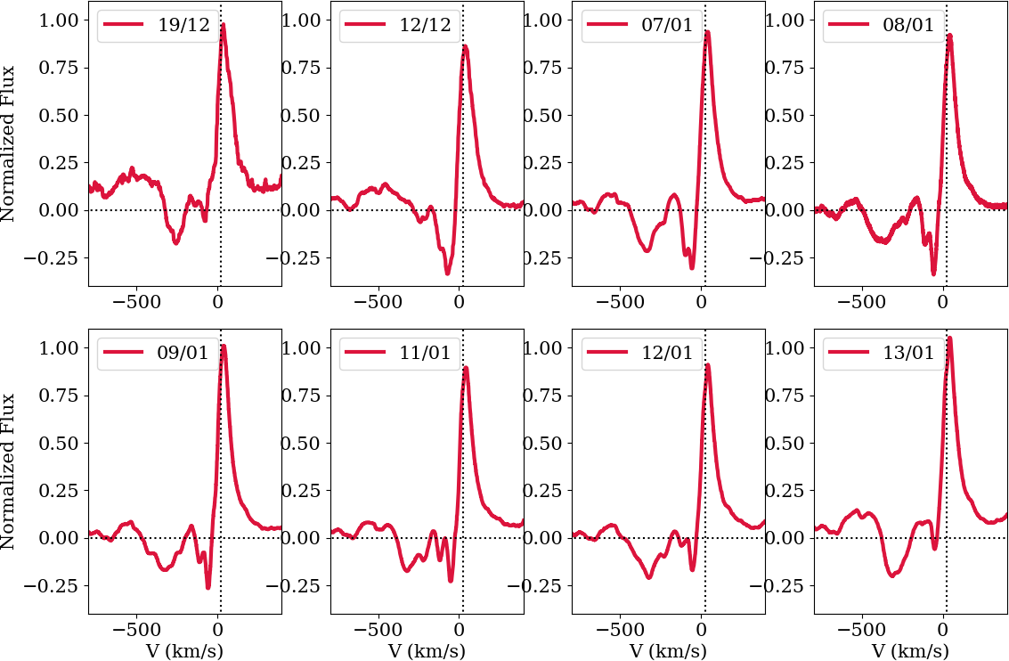
Figure 6: Examples of the time variability observed for the Ti II 4468Å line (left, blue), the Fe II 4923Å line (middle, green), and the Fe II 5316Å line (right, red). In each case, the 8 subfigures display the individual spectra as they were obtained in time. The dotted lines indicate the continuum level and the radial velocity of the source.

Variable and complex, strong winds are typical of quiescent early-type stars (Prinja, & Howarth, 1986). The many emission lines with P Cygni profiles are a sign of a powerful wind that gets stronger and more complex during outburst, which is typical of accretion outbursts and similar to what is observed in previous events (Covino et al., 1984; van den Ancker et al., 2004). At least three absorption components (at $-$900, $-$500 and $-$100 km s^-1) were reported by van den Ancker et al. (2004) during the 1999 outburst; the blueshifted absorption extended up to $-$1000 km s^-1 in the Balmer H series. According to Antoniucci et al. (2016), the wind from Z CMa NW is at least 20 times stronger than the FUor wind for velocities $-$90 to $-$400 km s^-1. This is confirmed by our quiescence spectra, which show much weaker absorption components despite having a higher proportional contribution from the FUor, and justifies our approach of treating the observed outburst lines as coming from Z CMa NW. The analysis of the quiescence wind is thus limited to pointing out the differences with outburst, since the quiescence data have an unknown contribution of Z CMa SE.

In our 2008/2009 data, the absorptions in the strongest Balmer lines are highly saturated and the wind is stronger than in the past, consistent with the 2 mag rise experienced in the 2009 outburst compared, for instance, to the 1 mag rise in 1999. The wind affects preferentially the high-energy lines, which is a sign of high wind temperature. The absorption features have complex and highly variable, high-velocity profiles, up to $-$800 km s^-1 in certain lines. The velocities of the fast and intermediate-velocity winds ($-$100 to $-$500 km s^-1) are similar to escape velocities in the innermost regions of the system ($<$0.1-0.3 au), which is consistent with stellar winds; these winds are associated with innermost accretion structures or initially poorly collimated launching regions that become the large-scale collimated jet. Since hotter temperatures are more likely to originate closer to the star, the high-velocity wind is the best candidate for a stellar or innermost-disk wind, while the low-velocity wind could originate in a disk wind.

Inner disk winds can explain the deep and broad absorptions observed in FUors (Milliner et al., 2018), which are similar to what is observed for Z CMa in the higher energy lines. He I and Si II are peaked toward the fastest wind components at $>-$400 km s^-1 (see Figure 2), indicating a very high temperature. He I and energetic lines may come from a more direct view (hotter, denser, saturated) than the Fe II and Ti II lines, which can also explain the differences in wind velocity and maximum redshifted velocities in the emission part of the PCygni profiles. The O I 8446Å line shows fast and slow components similar to Fe II lines, such as the Fe II 5018/4923 Å multiplet, maybe due to pumping by UV lines (e.g., H₂ C-X0-2Q(10) line; Herczeg et al., 2005). The absorption components observed in the optical lines are also in agreement with the large-scale jet observed around Z CMa NW, which have velocities from $-$450 to $-$600 km s^-1 (Whelan et al., 2010; Antoniucci et al., 2016). Ti II lines, which typically trace material at lower temperatures and densities, are dominated by the intermediate and slow wind.

The redshifted emission peaks of most strong ionized lines also suggest a slower wind around $-$20 km s^-1. The velocity of the slow wind is comparable to the escape velocity at $\sim$10-30 au, which is beyond the disk region detected in emission lines, but the orbital period at this distance is too long to expect significant day-to-day modulations, unlike what is observed.

Variations in the velocity of the absorption components are observed in all lines with non-saturated PC profiles, including those that have only a low-velocity absorption component, so that all wind components are variable. The day-to-day variations of the wind components could be caused by real variability, rotation, and/or small-scale occultation events in the innermost regions. Rapid variability in a high-velocity wind component has been also observed for ASASSN-13db in outburst, caused by rotation of an accretion-powered, non-axisymmetric wind (Sicilia-Aguilar et al., 2017). A difference in inclination angle can cause a variation in the absorption versus emission parts of the wind (e.g., Milliner et al., 2018), therefore we may observe material at multiple inclinations depending on the temperature structure.

The variability of the wind shows a clear time evolution. This is particularly evident for the six spectra taken on consecutive nights between 2009 January 7 and 13 (Figure 6). To examine these spectra, the various absorption components were locally fitted by Gaussians, considering their centers as the representative velocity of each individual wind component. This fit is a simple approximation, not taking into account other effects (e.g., optical depth, radiative transfer). Figure 7 shows that the Fe II and Ti II absorption profiles vary in parallel, even if their central velocities differ, which may arise from different line opacities (Sicilia-Aguilar et al., 2015). If we consider the Fe II 5316Å and Ti II 4468Å lines as examples, the Fe II very fast, broad wind component (with velocities between $-$300/$-$380 km s^-1) is the most variable and does not display a well-defined trend (besides not being observed in the lower energy Ti II lines). The intermediate-velocity wind component at $-$95/$-$120 km s^-1 and the slower wind component at $-$47/$-$55 km s^-1 are correlated for both lines (correlation coefficient 0.90, with false-alarm-probability 0.04 using a Spearman rank test) and vary smoothly with time, revealing the development and evolution of each individual component during the six observations.

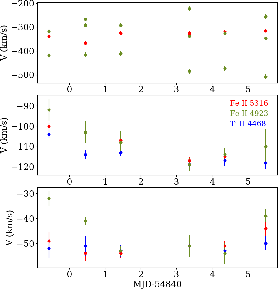
Figure 7: Day-to-day velocity variation of the wind components in 2009 January, classified according to the central velocities as very fast (top, observed clearly only for Fe II), fast (middle), and slow (lower). Results for the Fe II 5316 (red), Fe II 4923 (green), and Ti II 4468Å (blue) lines, which have good S/N and no signs of contaminations, are shown. The velocities are given as measured, without correcting for the radial velocity of the system. The correlations between the components observed for both intermediate velocity and slow wind lines, despite some shifts in velocity, are shown. The fast wind component appears to split into several components for some dates for the Fe II 4923Å.

Table 2: Lines selected for the Saha analysis, including the NIST data quality flag.

Species	$\lambda$	Aki	gk	gi	Ei	Ek	NIST	Comments
	(Å)	(s-1)			(eV)	(eV)	flag
FeI	5216.27	3.47E+05	5	5	1.608	3.984	A
FeI	5455.61	6.05E+05	3	3	1.011	3.802	B+
FeI	5506.78	5.01E+04	7	5	0.990	3.241	A	Some odd results
FeII	5627.50	2.90E+03	6	8	3.387	5.589	C	Potential blend
FeII	6084.10	3.00E+03	8	10	3.199	5.237	E
FeI	6256.36	7.40E+04	9	9	2.453	4.435	C
FeI	6265.13	6.84E+04	7	7	2.176	4.154	B
FeI	6358.63	5.19E+05	7	7	4.143	6.092	C+	Blend likely
FeI	6393.60	4.81E+05	9	11	2.433	4.371	C
FeI	6400.00	9.27E+06	9	7	3.603	5.539	B
FeI	6421.35	3.04E+05	5	5	2.279	4.209	B
FeI	6462.73	5.60E+04	9	9	2.453	4.371	C
FeI	6750.15	1.17E+05	3	3	2.424	4.260	B

Two scenarios are possible. The first would be rotational modulation of the wind (either in a stellar or disk wind), as it has seen in the multiple system GW Ori (Fang et al., 2014) and in the outbursting star FU Orionis (Powell et al., 2012) and ASASSN-13db (Sicilia-Aguilar et al., 2017). The wind modulation in GW Ori is caused by a companion, but any process resulting in a non-axisymmetric wind associated with either the star or the disk can produce the desired effect. The wind modulation in FU Orionis is periodic, which cannot be confirmed in this work due to the few spectra available. The second scenario would result from the propagation of a clump of matter along the wind. The radial velocities could vary due to changes in their angle with respect to the line of sight, as also occurs in the rotation scenario, or to changes in the physical velocity (e.g., in an accelerating wind). Both scenarios produce a smooth velocity evolution (as it is observed), but an accelerated wind would move toward larger velocities, while rotation would result in changes in the angle with respect to the line of sight. The variability ranges proportional to their velocity; the fast component changes by $\sim$25 km s^-1 and the slow wind component changes by $\sim$8 km s^-1 during these six day (see Figure 7). This is consistent with rotation and projection effects as observed in rapidly variable, winding winds in certain B-type stars (Prinja, & Howarth, 1986, 1988), where a rotating/spiraling, non-axisymmetric clumpy wind, moving not only radially, but also azimuthally, causes differences in opacity along the line of sight and thus rapid velocity variations. The trend extends to the very fast wind component observed in Fe II, although the error in its central velocity is large because the absorption features are very broad. Testing whether the system shows any periodic or quasi-periodic behavior in the wind velocity and strength can help to distinguish these scenarios.

The conclusions of this section are that Z CMa NW develops a hot, fast wind in outburst, which is likely of stellar or innermost disk origin, as well as colder components that could be related to the disk. The wind is variable on timescales of days, and the intermediate and strong, slow wind components are clearly correlated, betraying a small-scale structure and a clumpy nature in a rotating, non-axisymmetric wind.

3.3 Saha’s equation constraints on temperature and density in outburst and quiescence

We can use the observed emission lines to put constraints on the density and temperature of the emitting material, assuming LTE. We use Saha’s and Boltzmann’s equations (Appendix C.1) to derive expected intensities for a range of temperatures and densities and compare these with the observations. For velocity-resolved lines, it is possible to distinguish various gaseous structures considering their velocities. For Z CMa NW, where different lines are related to different physical structures (e.g. winds, hot inner disk, accretion structures), it is crucial to classify the lines according to their profiles. Most Fe II lines have P Cygni profiles, while Fe I lines have disk- or box-like profiles, a sign that they are not produced by the same structure and cannot be treated together. Many lines are saturated and probably originate in optically thick regions, so a proper fit would require full radiative transfer. As a result, the only cases for which we can apply this method are weak Fe I and Fe II lines with similar box- or disk-like profiles (see Table 2). There are only two clean Fe II lines with box-like profiles, $\lambda\lambda$ 5627.497, 6084.103Å. These lines have transition probabilities on the order of 1e3 s^-1 and are very weak. Among the clean Fe I lines, only four have low enough transition probabilities for the assumption of optically thin lines to be justified.

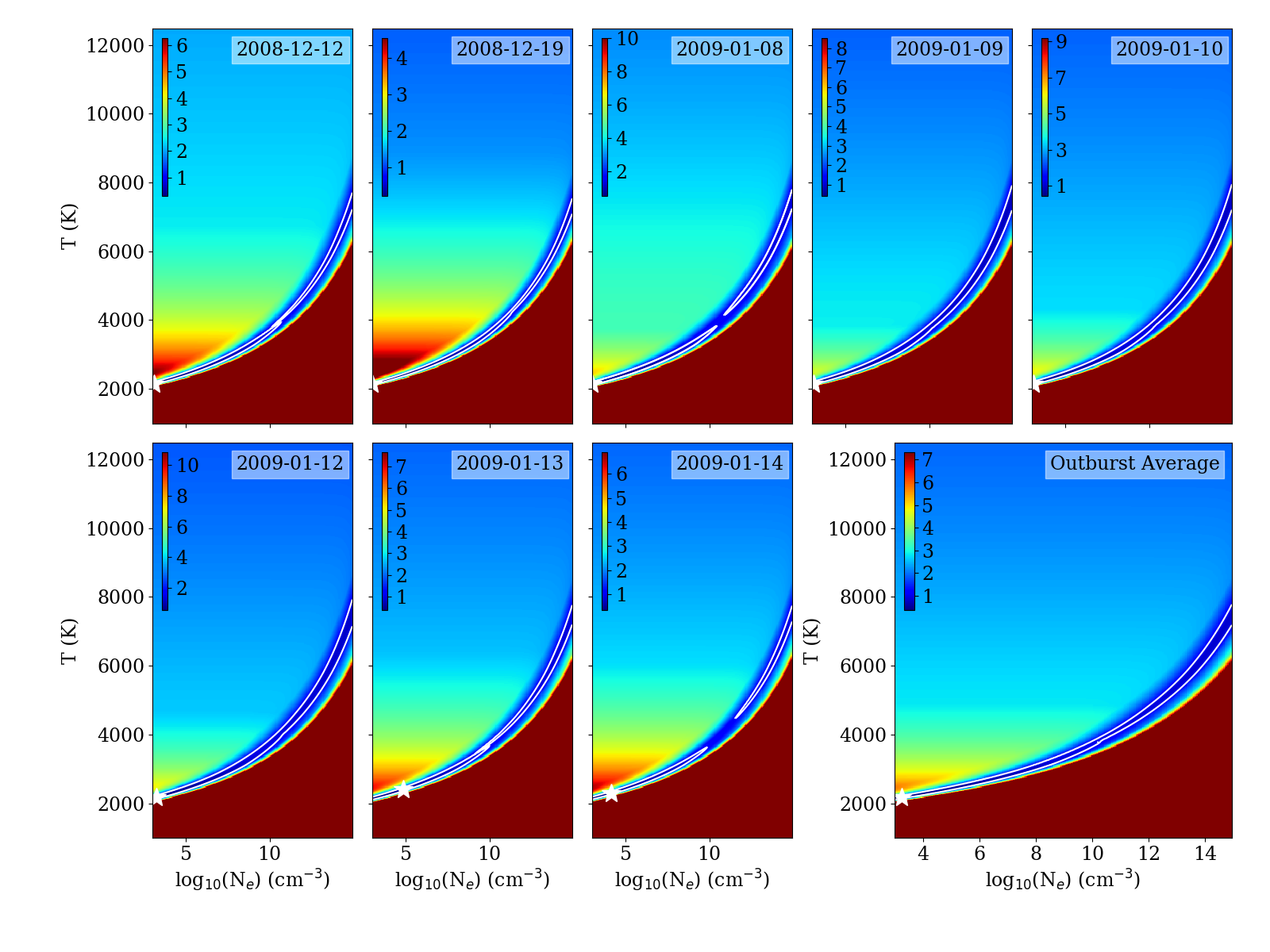
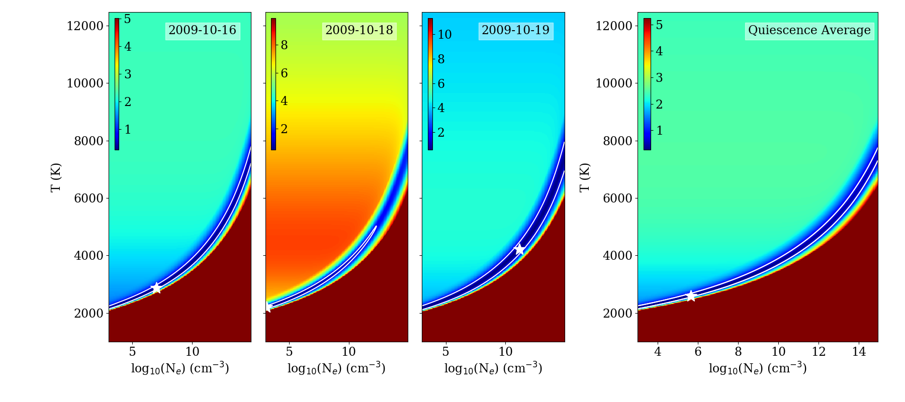
Figure 8: Result of Saha’s equation analysis for the lines with disk-like profiles and low transition probabilities for the observations taken during the outburst phase (upper panels) and for the same lines as observed during quiescence (lower row). The panels show the data corresponding to individual days in chronological order; the last panel shows the result of fitting the average spectrum. The color scheme reveals the relative variations in the line intensity ratio for each combination of temperature and electron density (such that 0.1 would correspond to 10% average deviations). The white contour indicates the regions for which the relative variations of the line ratio are up to 3 times the minimum value observed, which is considered as our best-fit region; a white star denotes the best fit.

The lines were extracted from the continuum and scaled to the same arbitrary-unit scale. Considering a reasonable range of temperatures and electron densities, we can estimate the relative line intensity expected depending on the physical conditions. Leaving the total density of Fe I as an unknown, the relative strength of Fe II lines with respect to Fe I lines is given by Saha’s equation (Eq. 9). Then, for each transition we consider the atomic parameters so that the total line strength is given by the transition probability (A_ki) divided by the wavelength and multiplied by the Boltzmann distribution (Eq. 10). We estimated theoretical line ratios for temperatures from 1000 K to 12500 K and electron densities 10³-10¹⁵ cm^-3. Saha’s equation has an intrinsic degeneracy between the electron density and the temperature, which means that higher temperatures with higher electron densities may reproduce the same line ratios, but we add further constraints in the following sections. The spectra are not flux-calibrated, and the theoretical intensity is calculated as a ratio of the intensities depending on the ratio of ionized to neutral elements, so the lack of scale invalidates the $\chi^{2}$ statistics (e.g., Andrae et al., 2010). Therefore, the best-fitting density is obtained by minimizing the standard deviation in the ratio of the observed to theoretical line intensities, taking the median of the ratio of the observed to theoretical lines as a scaling factor. The contribution of each line is weighted taking into account the uncertainties in its atomic parameters using the NIST data quality flag. To assess the uncertainties in the results, the exercise was repeated for each one of the eight outburst observations and for the average outburst spectrum. There are no significant differences between dates, thus the variations are due to noise.

The exercise can be repeated for the lines observed in quiescence, remembering that there is no evidence that quiescence lines originate in the disk. The data from 2009-10-18 suggest higher temperatures and densities than for the other quiescence spectra, which could be related to an increased accretion rate in either of the two Z CMa components. Although the H$\alpha$ emission line is strong on that particular day, the noise level is also higher and there are no other significant differences between all three quiescence spectra. Therefore, random noise cannot be fully excluded and the results from the averaged quiescence spectra may be more representative of the typical quiescence state.

Table 3: Results from the Fe I/FeII Saha line analysis.

Date	Tbest	Tmedian	Trange	ne,best	ne,range	Notes
	(K)	(K)	(K)	(cm-3)	(cm-3)
2008-12-12	2400	4050	2125-7725	7.1e4	1e3-1e15
2008-12-19	2300	4260	2125-7700	1.4e4	1e3-1e15
2009-01-08	2150	4600	2125-7775	1.3e3	1e3-1e15
2009-01-09	2150	4600	2125-7900	1e3	1e3-1e15
2009-01-10	2150	4600	2125-7925	1.3e3	1e3-1e15
2009-01-12	2150	4525	2100-7925	1.3e3	1e3-1e15
2009-01-13	2150	4625	2125-7750	1.3e3	1e3-1e15
2009-01-14	2175	4800	2125-7725	1.8e3	1e3-1e15
Outburst Average	2175	4525	2125-775	1.8e3	1e3-1e15
2009-10-16	2875	4560	2150-7775	1.0e7	1e3-1e15
2009-10-18	2200	3075	2150-5025	1.3e3	1e3-2e12
2009-10-19	4225	4550	2125-7950	1.4e11	1e3-1e15	Anomalous values
Quiescence Average	2600	4250	2150-7750	4.5e5	1e3-1e15

The explored range of electron densities and temperatures and the best-fitting values are shown in Figure 8. One warning regarding the interpretation of these results is that the deviations from the best-fit models for different groups of lines are not random. While neutral lines tend to favor a relatively low temperature (on the order of 2000-3000 K), to reproduce the ionized lines at the same level we tend to require higher temperatures and densities ($\sim$7600 K) and the best fit tends to the lower temperature values because the atomic parameters of the neutral lines have smaller uncertainties. There are no perfect fits and, in particular, the FeI line at 5506Å and the FeII line at 6084Å, which has a particularly large uncertainty in its atomic parameters, are usually badly fitted (within a factor of $\sim$10) by any combination of temperatures and electron densities that reproduces the remaining lines. As observed in EX Lupi (Sicilia-Aguilar et al., 2015), this may indicate multiple components with various densities and temperatures, although for Z CMa there are too few weak Fe II lines to attempt a more complex model fit. Despite the uncertainties and degeneracy, the best fits suggest a relatively low temperature for the formation of the observed disk-shaped lines. The constraints on the density are weaker, although the best-fitting values tend toward the lower end as well (see Figure 8). Although we cannot use the Ti I/Ti II lines for this exercise because all the Ti II lines are heavily affected by the winds, we note that the temperature and density ranges obtained from Fe I/Fe II are consistent with the strongest Ti I lines having rounded or narrow profiles. These lines are very sensitive to temperature, disappearing for temperatures more than 3000 K at the observed best-fit densities. The fact that no disk-like profiles are observed for Ti I lines suggests that they may come from regions in the disk at larger radii (and thus colder) than the Fe I lines. Therefore, this section adds an additional proof of the inner disk emission being extended, which agrees with the range of temperatures required to explain both the Fe I and Fe II emission (from 2000-3000 K to 7000 K) and with the variety of observed disk-like profiles. The narrow quiescence lines may be linked to the accretion structures in quiescence.

Table 4: Lines that share a common upper level, among those with disk-like profiles.

Species	$\lambda_{0}$	Aji	Uncertainty	Notes
	(Å)	(s-1)
FeI	4786.8, 5262.9	1.03E+06, 8.70E+04	50%	Second one blended/uncertain
FeI	4839.5, 7511.0	3.90E+05, 1.35E+07	18%	Uncertain continuum (7511), blends
FeI	4939.7:, 5051.6, 5142.9	1.39E+04, 4.65E+04, 2.40E+04	40%	Blends
FeI	4957.6, 6271.3	4.22E+07, 3.05E+04	18%	Blends
FeI	5141.7, 6270.2	4.86E+05, 1.39E+05	50%	Blends
FeI	5393.2, 5615.6, 5709.4	4.91E+06, 2.64E+07, 2.13E+06	18%	Blends
FeI	5543.9, 5641.4	3.40E+06, 3.00E+06	50%	Strength too similar, uncertain
FeI	5572.8, 5624.5, 6408.0	2.28E+07, 7.41E+06, 3.12E+06	10%	OK first two lines
FeI	5747.9, 6103.3	8.80E+05, 1.52E+06	50%	Blends, uncertain
FeI	6191.6, 6256.4	7.41E+05, 7.40E+04	25%	OK
FeI	6393.6, 6462.7	4.81E+05, 9.70E+04	25%	OK
FeI	6265.1, 6335.3	6.84E+04, 1.58E+05	18%	Blends
FeI	6750.2, 8674.7, 8838.4	1.17E+05, 6.17E+05, 3.83E+05	25%	Strength too similar, uncertain

3.4 Line ratio constraints on the disk and wind properties

Here, we follow Beristain et al. (1998) to derive the optical depth of the line-emitting disk material using lines that share the same upper level. This avoids having to deal with the way the upper level is populated, so that the resulting relative intensities depend only on the atomic parameters, temperature, and line opacity. For velocity-resolved lines, we can apply the Sobolev approximation to write down the line opacity, which results in the line strength depending only on the atomic parameters, temperature, and column density-velocity gradient ($ndv/dl$, where $n$ is the density, $v$ is the velocity, and $l$ is the spatial scale). The details of the procedure are given in Appendix C.1. We first apply this method to the disk-like emission lines, and then examine the results for the lines with P Cygni profiles.

3.4.1 Line ratio constraints on the inner disk

There are 13 groups of lines from the same upper level among the disk-like lines (Table 4). Nevertheless, only 3 groups remain for which the lines are not blended, are close enough to minimize the effects of the continuum variations, and have high-quality NIST atomic data. A fourth pair, Fe I $\lambda\lambda$ 8674.7, 8838.4 Å, also satisfies the above conditions, but the presumably stronger line is observed to be weaker. This is probably caused by the 25% uncertainty in the transition probabilities plus the fact that both lines have a very similar strength. Considering the uncertainties, the best line pair is Fe I 5572/5624 Å (10% uncertainty or class B, compared to 25% uncertainty for the other two pairs). The smaller difference between the transition probabilities for the Fe I 6393/6492 Å pair makes it the least constrained. All three line pairs are also detected in quiescence, but the Fe I 5572/5624Å pair in quiescence is too weak to be used.

Outburst	Quiescence

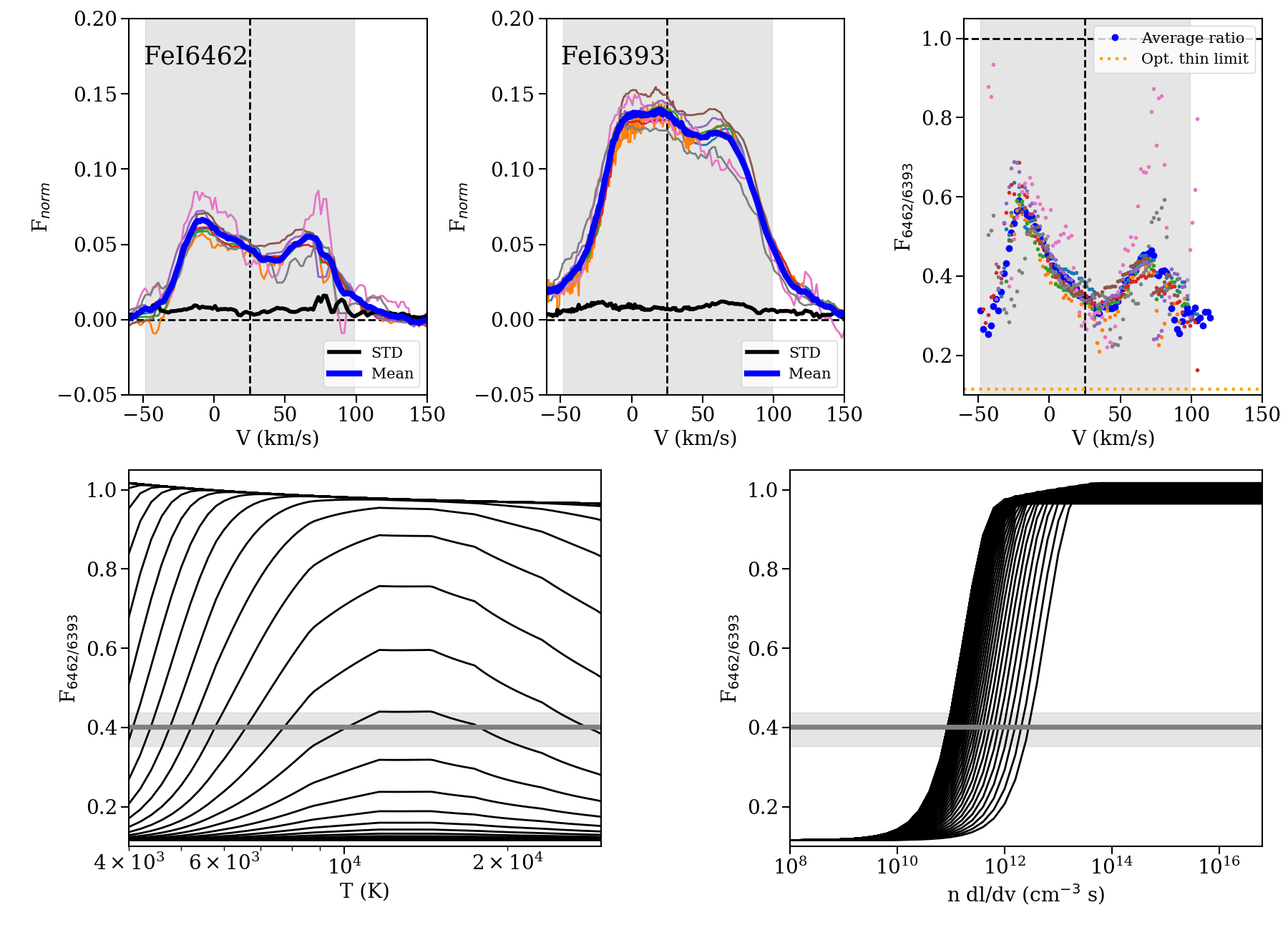
Figure 9: Analysis of the line ratio for Fe I transitions with common upper levels (continued in Appendix C). The upper left panels show the line emission in outburst and the upper right panels show the quiescence data. The ratios observed are compared to the theoretical calculations for a range of temperatures and column density-velocity gradients in the lower panels. The gray area shows the region for which the line emission is $>$5$\sigma$ (in the velocity panels) and the 1$\sigma$ error in the temperature and density planes. Quiescence lines are often very weak and thus uncertain.

To derive the ratios, we normalized every line individually. First, the global shape of the spectrum has to be taken into account, which for lines that have similar wavelengths can be done assuming a linear fit between the two regions. We imposed a minimum of 5$\sigma$ emission above the noise level to obtain the ratio, where $\sigma$ corresponds to the standard deviation of the flux measured in a line-free nearby region, to avoid unphysical values due to noise. We analyzed the outburst spectra individually, together with the averaged spectrum, to estimate the noise and variability. For comparison, we also analyzed the quiescence data in the same manner, which is discussed in Section 3.6.

The results are shown in Figure 9 and continued in Appendix C. All figures show the velocity-by-velocity line ratio, followed by a comparison with models covering a range of temperature and velocity-density gradient going from the conditions where both lines are optically thin, to the strong line saturating, and finally, to the limit where the two lines are saturated (Beristain et al., 1998). Leaving aside the Fe I 5572/5624Å pair that is close to saturation in the line wings as well as the center, the central part (closer to zero velocity) appears to be optically thinner than the high-velocity wings in the outburst lines. For a disk scenario, this can be explained if the density decreases toward larger radii (lower velocities), which is reasonable. For the quiescence data, the emission is close to being optically thin in the weak line for both the Fe I 6256/6191Å and the Fe I 6462/6393Å pairs. This is significantly different from what has been observed in EX Lupi (Sicilia-Aguilar et al., 2012, 2015) and DR Tau (Beristain et al., 1998), where narrow lines are optically thicker than the broad components and can be traced back to dense, hot spots on the stellar surface, and suggests a disk origin.

We can combine all of the lines to derive a better constraint on temperature and density (see Figure 10). The temperature is not too well constrained from this exercise, but most of the lines agree with column density-velocity gradients ($ndl/dv$) on the order of 10¹⁰-10¹² cm^-3s, higher than in quiescence. The weakness of the lines, the uncertainty of some of the atomic parameters, and the potential breakdown of the Sobolev approximation for lower velocity gradients may cause part of the temperature mismatch between line pairs. If we combine this result with Saha’s equation from the previous section, both converge toward larger densities and lower ($\sim$4000-5000 K) temperatures, which is also consistent with the origin in a disk and the values derived from the lines with lower uncertainties.

A limitation of this procedure is that lines with various strengths (and line profiles) trace material originating in slightly different locations, which adds a further uncertainty. The line pairs examined to trace the disk emission during outburst have typical ratios in between the optically thin and optically thick limits. This means that the weak line is usually optically thin, while the strong line is optically thick. The optically thin line probes material deeper into the disk, which explains why lines with low transition probabilities look more disk-like (instead of box-like) than lines with high transition probabilities. In addition, narrow-line components (originating in more compact but relatively hot and dense regions, such as hot spots at the stellar surface or in the accretion shock region) would be stronger for the lines with high transition probability because low transition probability lines would be more susceptible to collisional deexcitation in these environments. Such departures from disk-like profile related to optical depth are also observed in CO lines (e.g., see Panić et al., 2008; Hein Bertelsen et al., 2016; Carmona et al., 2017), contributing to the box-like appearance of optically thick lines. As in such cases, Fe I lines with various optical depths can give information concerning the vertical temperature structure. In the case of the strong lines, the box-like features would not result from optically thick material in a flat disk (e.g., as in the examples from Horne & Marsh, 1986), but rather from material coming from various layers and distances in the optically thick, flared disk. In addition, contributions from a disk wind can affect the double-peaked profiles in optically thick lines, and can, together with optical depth, result in box-like profiles (Murray & Chiang, 1996, 1997; Ferguson, 1997). Wind can quickly overwhelm disk (and magnetospheric) emission due to its larger volume (Tambovtseva et al., 2016), which is not observed here.

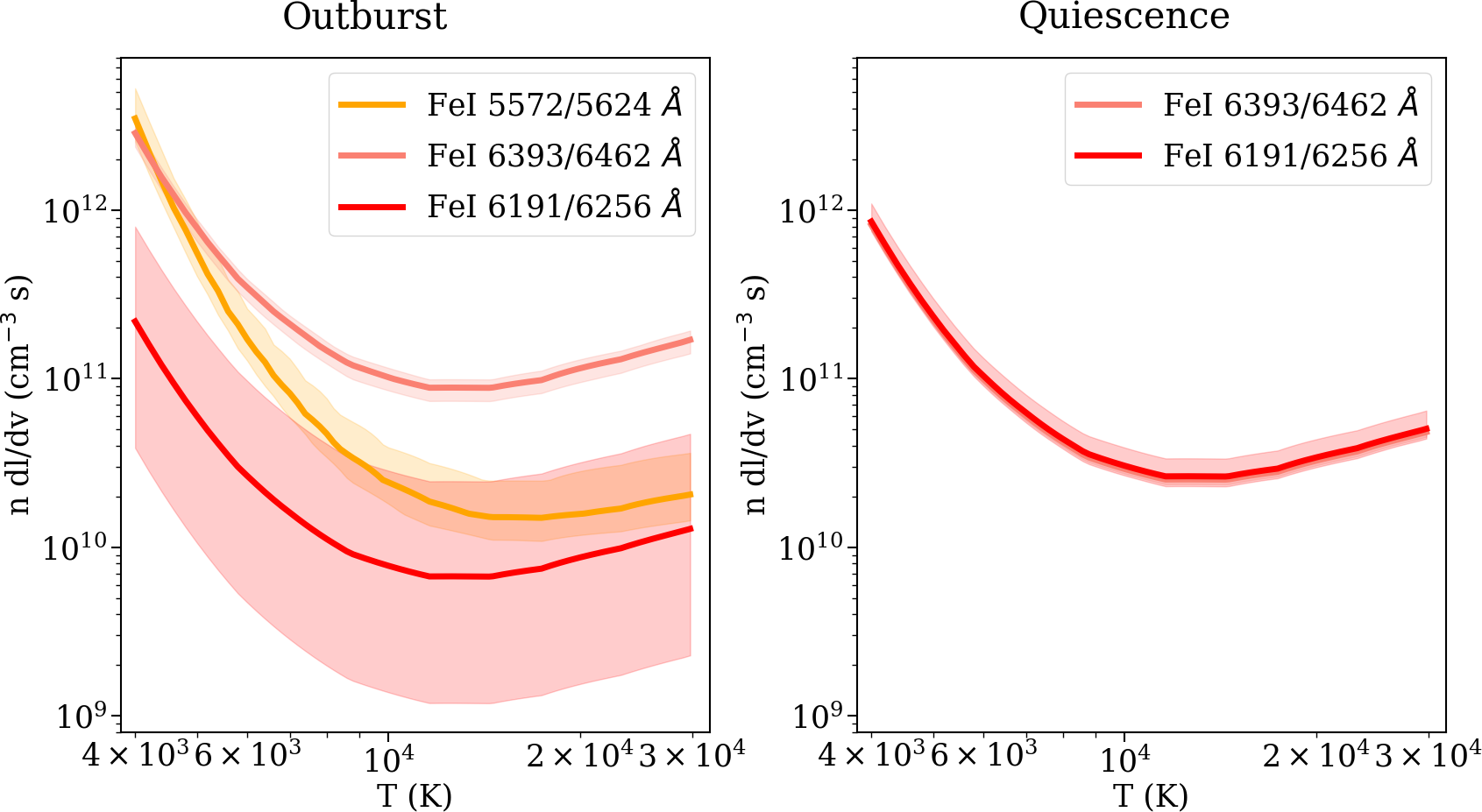
Figure 10: Result of the line ratio analysis for neutral lines with disk profiles in outburst (left) and narrow profiles in quiescence (right).

Most of the observed disk lines are systematically brighter on their blue side. This blue-red asymmetry could be due to inclination and flaring—the red and the blue parts may appear to have different inclinations; (Hein Bertelsen et al., 2016)—a density enhancement on the blue side, an off-center disk, or contamination by other contributors to the line emission such as accretion structures or the disk wind, which does not need to be uniform. We further examine the location of the emitting material based on the velocities in Section 3.5, but the results are consistent. A blue asymmetry, likely related to wind, is also observed, albeit in absorption, in the strongest disk-like lines in FU Ori (Donati et al., 2005).

The column density-velocity gradients can be used to estimate the densities and constrain the values derived from Saha’s equation. Considering that the maximum $dv/dl$ is given by approximately $v/r$ where v and r are the Keplerian velocity and radius, the best-fitting column density-velocity gradient of 1e12cm^-3s suggests a particle density at least 3e4 cm^-3. This value is clearly lower than our estimate for the accretion structures (Section 3.1), which is consistent taking into account that the disk is likely less dense than the accretion channels, especially at larger radii. Together with the temperature derived from this procedure ($\sim$4000-5000 K), this section confirms the agreement of the neutral line emission with an origin in an extended disk structure around the star as well as a density (optical depth), radial differences between the high-velocity disk (line wings, formed closer in), and the lower-density, lower-velocity regions (related to the outer disk).

3.4.2 Line ratio constraints on the wind absorption and redshifted emission components

Table 5: Lines with PCygni profile that share a common upper level.

Species	$\lambda_{0}$	Aji	Uncertainty	Notes
	(Å)	(s-1)
HI	3750.151, 8750.46	2.83e+04, 2.02e+04	1%	Complex continuum
HI	3797.909, 9015.300	7.1225e+04, 5.1558e+04	1%	Telluric cont.
TiII	3900.540, 5129.150	1.60E+07, 1.00E+06	50%	OK
FeII	3938.290, 6432.680	6.10E+03, 8.50E+03	50%	First line blend
FeII	4128.748, 4303.176, 4522.634	2.60E+04, 2.20E+05, 8.40E+05	50%	Blends
FeII	4178.862, 4520.224, 5276.002		50%	Blends
FeII	4233.167, 4731.453	1.72E+05, 2.80E+04	50%	OK
FeII	4258.154, 5197.577	3.10E+04, 5.40E+05	50%	First line blend
FeII	4273.326, 4508.288	9.10E+04, 7.30E+05	50%	Blends
FeII	4296.652, 4489.183, 5234.625	7.00E+04, 5.90E+04, 2.50E+05	50%	Blends
TiII	4443.800, 4450.490, 4501.270	1.1E+07, 2.00E+06, 9.80E+06	50%	Blends
FeII	4629.339, 4666.758	1.72E+05, 1.30E+04	25%	OK
TiII	4779.985, 4805.100	6.20E+06, 1.10E+07	50%	OK
FeII	6238.375, 6247.562	7.50E+04, 1.60E+05	50%	OK
OI	7771.940,7774.170, 7775.390	3.69e+07	3%	Blends

Outburst	Quiescence

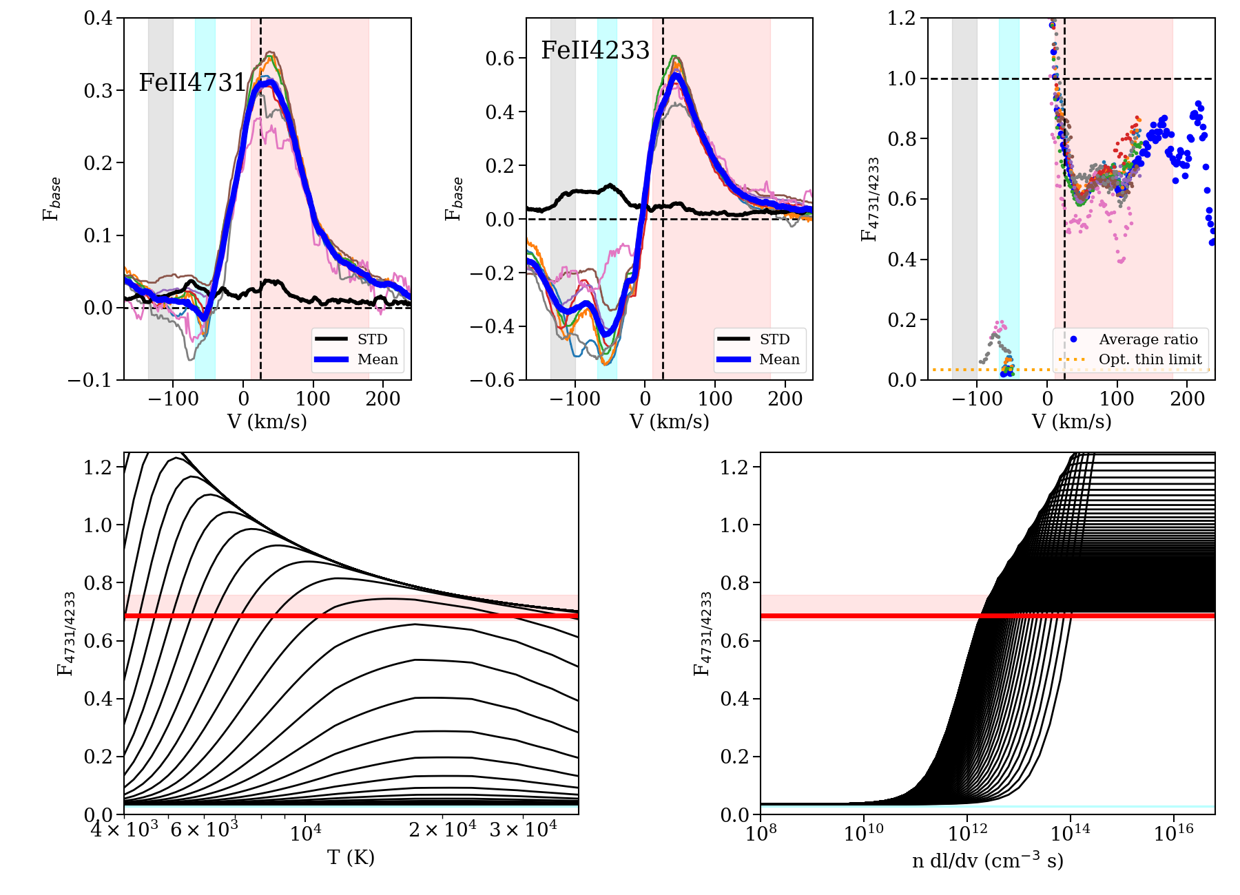
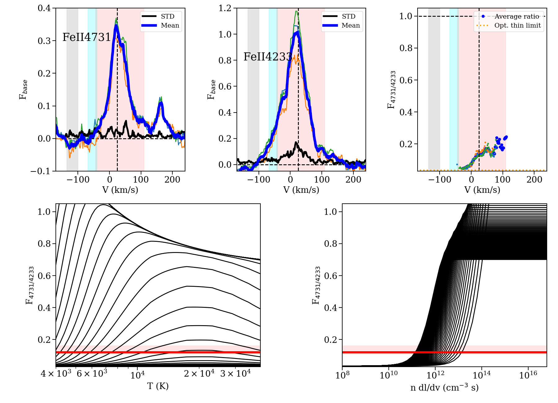
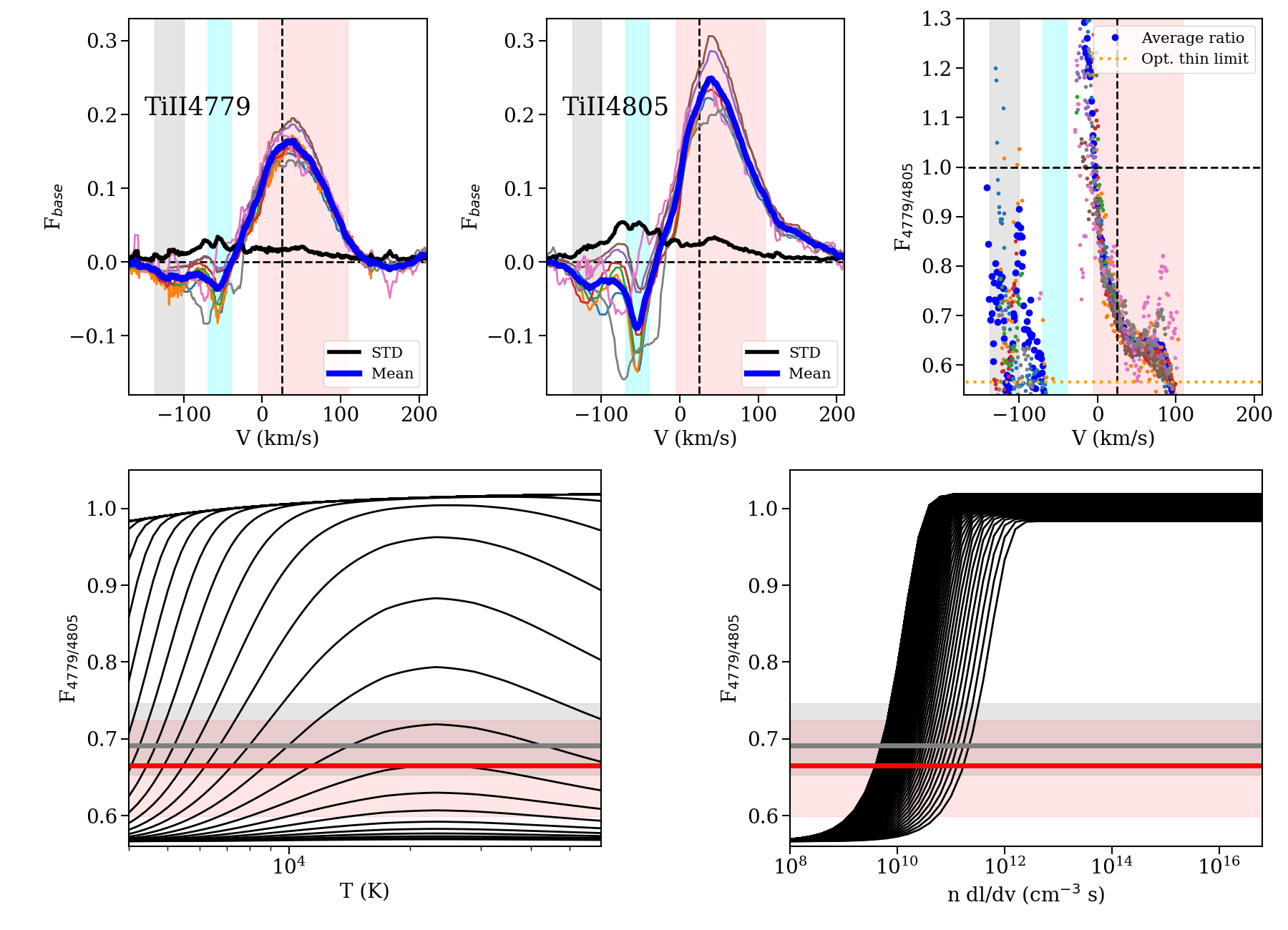
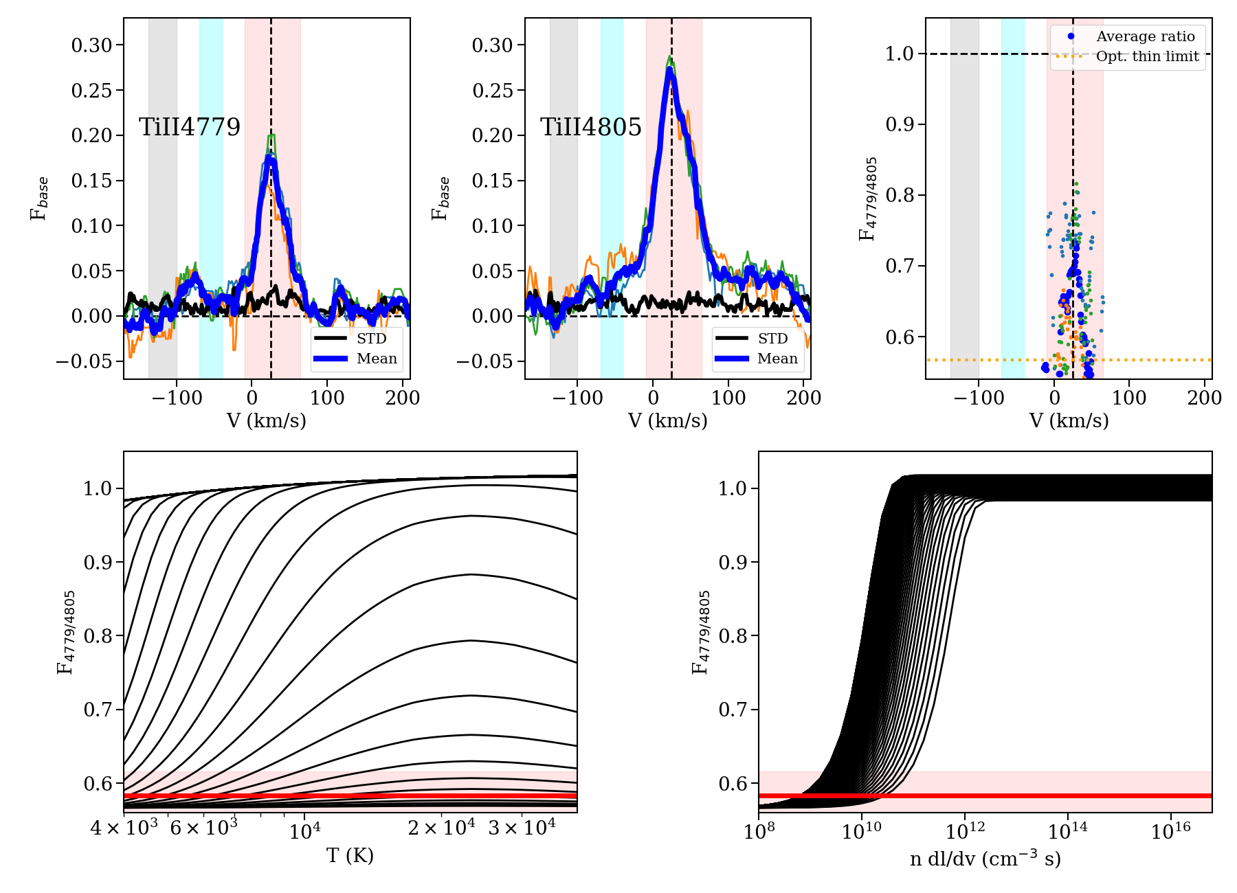
Figure 11: Analysis of the line ratio for the FeII and TiII lines with PCygni profiles from transitions with common upper levels (continued in Appendix C). The upper left panels show the line emission in outburst and the upper right panel shows the quiescence data. The ratios observed are compared to the theoretical calculations for a range of temperatures and column density-velocity gradients in the lower panels. In the velocity panels, the red, cyan, and gray areas show the regions with significant redshifted emission and slow and fast wind absorption, respectively. The shaded colored areas in the temperature and density planes show the regions that are compatible with the line ratios observed in the emission and the two wind component parts with their 1$\sigma$ error. See text for details.

The same exercise of line ratios was done for the pairs of lines with wind signatures that share an upper common level. We find a total of 15 pairs or triplets of lines with common upper levels and P Cygni profiles (see Table 5), but only 5 pairs remain if we exclude pairs. For the line ratio analysis, we checked both the line ratio in the emission part (measured as positive over the continuum) and in the absorption part (measured as negative under the continuum). The velocity space was divided in the region in which both lines have significant ($>$5$\sigma$) emission and the regions in which both lines have significant absorption. The ratio was only calculated where both lines were either in emission or in absorption. The wind was separated in two components, the fast and the slow wind, but since the emission part of the lines is very broad, it is very likely that the slow wind is contaminated by emission. This explains the unphysical ratios observed at some velocities. The line pairs show no significant absorption during quiescence, a signature of the wind becoming optically thin, as expected from an accretion-powered wind.

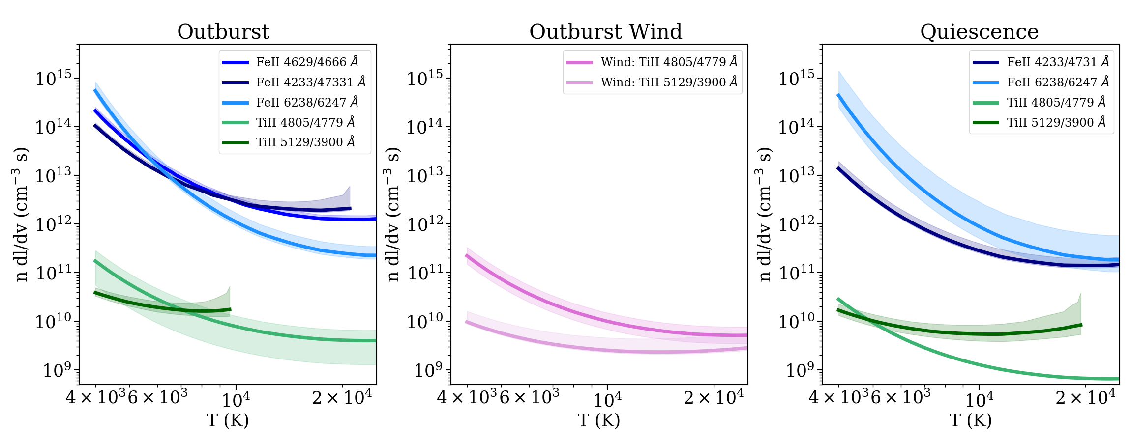
Figure 12: Result of the line ratio analysis ion pairs of lines with a common upper level for the emission and wind absorption parts (denoted as ”wind” in the legend). Some of the Ti II lines have sharp cuts in the n dv/dl vs. T plane due to unphysical values that arise in regions of low S/N (see Appendix C). The results have to be regarded with care when approaching such regions.

Figure 11 shows the results. The wind components cover a large range of temperatures and densities. We can put together the column density-velocity gradient and temperature ranges favored by each line ratio to get a better constraint for both the emission and fast wind (Figure 12). Since the wind absorptions are very weak for all the line pairs, derived wind properties are strongly affected by the noise. Weak lines with low transition probabilities have very weak or even absent absorption, a signature of being optically thin. This constrains the maximum density allowed for a given wind temperature and the range of densities that this method can probe. For the emission component of the line, both the Fe II line pairs and Ti II line pairs are consistent with a temperature in the range 6000-7000 K, although the Ti II lines favor a column density-velocity gradient value three orders of magnitude lower. Given that the line profiles for Fe II and Ti II are not identical, differences in the physical location are expected. Only the two Ti II pairs give significant results for the fast wind component, suggesting a much lower column density-velocity gradient and a very high temperature ($>$2e4 K). Since the uncertainties in the atomic parameters for Ti II are $\sim$50%, the final results have uncertainties on the order of 70%, which would be compatible with a lower bound temperature of $\sim$ 10⁴ K. Such large temperatures are more consistent with a stellar, rather than a disk wind, origin. The relative values for the Ti II lines suggest that the column density-velocity gradient is between 1 and 2 orders of magnitude lower for the wind than for the redshifted (potential infall-related) part.

The emission part of the line has a narrow, central component in the weakest ionized lines, probably because the strong lines with large transition probabilities are highly saturated. The lack of narrow components in low transition probability neutral lines is likely related to temperature: the originating accretion structure, wind, or hot spots in the proximities of the star are likely too hot to allow for strong Fe I emission. If the temperatures are low enough to ensure that the metals are all once-ionized and hydrogen remains neutral, the electron density would be approximately 0.1% of the hydrogen number density. Typical redshifted velocities in the metallic lines are around 100 km s^-1, which is likely too low to be explained by free fall around an intermediate-mass star, but compatible with, for example, rotation at a few stellar radii. The 10¹³ cm^-3s^-1 column density velocity gradient constrained by the line ratios would then result in electron densities on the order of 10⁵, which require temperatures of at least 3500 K to avoid Fe I emission (according to Saha’s equation). The temperatures from line ratios are about a factor of 2 higher (see below), explaining the lack of Fe I emission with accretion or wind signatures and the scarcity of Fe II lines with disk profiles.

The temperatures of the redshifted wings derived from the line pairs are around 7000 K, which are low for an origin in the accretion columns in the proximity of a luminous, intermediate-mass star. This suggests that the lines originate in a more distant region, inconsistent with magnetospheric accretion; infall velocity onto an intermediate-mass star would rapidly exceed the 100-200 km s^-1 ranges observed in the line wings. A boundary layer scenario also fails to explain the velocities in the inner disk, which are expected to be significantly lower than observed in disk-like lines (Popham et al., 1993), although increased velocities due to turbulence may reach a few 100 km s^-1 (Bertout et al., 1988). As in the disk analysis, because optical spectra trace relatively low-energy lines, we have a selection bias toward lower temperatures. This could explain their origin not too close to the star, so we may be indeed missing the hottest, highest velocity emission in most of these line pairs. Much higher velocities, more consistent with infall on an intermediate-mass star, are seen in the very extended wings of the H Balmer lines. A hotter and higher-velocity region could be explored further with spectroscopic observations covering metallic UV lines.

Summarizing, line ratios reveal a highly structured wind and a complex origin for the redshifted emission components. Both cover a broad range of densities and temperatures that can be probed by lines with various excitation energies. The wind temperatures are consistent with a stellar (or innermost disk) origin, while the redshifted emission could originate at a few stellar radii. The wind becomes optically thinner in quiescence, which is consistent with being powered by accretion.

3.5 Disk structure derived from the velocity analysis

Table 6: Summary of the brightness decomposition of lines with disk-like profile.

Species/$\lambda_{0}$	Aki	Ek	vrad	Vp2p	FWHM	Notes
(Å)	(s-1)	(eV)	(km s-1)	(km s-1)	(km s-1)
FeI 5506.8	1.14E+08	3.241	26.9$\pm$0.3	78$\pm$6	113$\pm$23	Blue-dominated, no high-velocity wings.
FeI 5572.8	2.28E+07	5.621	35.8$\pm$0.3	72$\pm$4	115$\pm$2	Very disky, no high-velocity wings, some central emission.
CaI 5598.5	4.30E+07	4.735	21.3$\pm$0.6	81$\pm$2	113$\pm$3	Small blue wings.
FeI 5615.6	2.39E+05	5.539	26.2$\pm$0.1	62$\pm$1	120$\pm$1	Strong high-velocity wings.
FeI 5624.5	8.30E+05	5.621	30.2$\pm$0.1	74$\pm$2	105$\pm$2	Strong blue high-velocity wing.
FeI 6065.5	1.07E+06	4.652	31$\pm$1	74$\pm$2	119$\pm$3	Strong high-velocity wings, mostly blue.
NiI 6108.1	1.30E+05	3.706	24.5$\pm$0.8	55$\pm$3:	95$\pm$2	Very asymmetric, red side may be absorbed by nearby feature.
FeI 6256.4	7.40E+04	4.435	30$\pm$3	87$\pm$1	108$\pm$11	Disk-like, but has low S/N and nearby absorption lines.
FeI 6265.1	6.84E+04	4.154	36.9$\pm$0.1	76$\pm$4	108$\pm$2	Clean, no wings.
FeI 6358.6	5.19E+05	6.092	36$\pm$1	81$\pm$5	107$\pm$14	Low S/N and asymmetric continuum due to nearby lines.
FeI 6393.6	4.81E+05	4.371	23.5$\pm$0.5	62$\pm$2	115$\pm$1	Asymmetric, may have an additional blueshifted absorption.
FeI 6400.0	9.27E+06	5.539	37.5$\pm$0.3	79$\pm$2	118$\pm$2	High-velocity wings.
FeI 6411.6	4.43E+06	5.587	41$\pm$1	82$\pm$17	107$\pm$15	Red-dominated.
FeI 6421.4	3.04E+05	4.209	29.1$\pm$0.3	73$\pm$22	109$\pm$2
CaI 6439.1	5.30E+07	4.103	27$\pm$1	82.5$\pm$0.8	111$\pm$15	Blue-dominated, very strong high-velocity blue wing.
FeI 6462.7	5.60E+04	4.371	25.9$\pm$0.6	75$\pm$2	113$\pm$2
CaI 6717.7	1.20E+07	4.554	27.4$\pm$0.9	74$\pm$2	124$\pm$4	Asymmetric continuum.
FeI 6750.2	1.17E+05	4.260	25$\pm$0.1	80$\pm$1	107$\pm$17	Very extended high-velocity wings to red and blue parts.
NiI 6767.8	3.30E+05	3.658	27.9$\pm$0.8	79$\pm$1	109$\pm$2	Blue high-velocity wing.
FeI 8674.7	6.17E+05	4.260	37.6$\pm$0.6	78$\pm$2	108$\pm$4	Flat-top.
FeI 8824.2	3.53E+05	3.603	31.1$\pm$0.3	68$\pm$1	121$\pm$2	High-velocity wings, central narrow emission.
FeI 8838.4	3.83E+05	4.260	34.9$\pm$0.4	80.1$\pm$0.7	114$\pm$3

We used the brightness decomposition technique from Acke & van den Ancker (2006) to study the velocity structure of the disk-like lines. The details of the procedure are given in Appendix C.2. For lines with disk-like profiles, the highest velocities are caused by material in the innermost disk. Starting with the highest velocity, we fit a ring that can reproduce the observed flux and subtracted it from the line profile, repeating the procedure until the line is entirely fitted or we reach a velocity in which emission from narrow, non-disk components dominates. The emission scales as a blackbody with temperature given by a power law of the radius. The final emission is obtained by summing all rings. All the observed lines are best fit using the temperature power law for a flared, irradiated disk model (D’Alessio et al., 1999). Given that the accretion during the outburst is very high, to account for an irradiated disk at few astronomical units we need the bulk of the accretion energy to be released closer to the star than the region that produces the disk-like lines, at a fraction of an astronomic unit or less, or radii smaller than those inferred from the lines with disk profiles, justifying our discussion in Section 3.1. Some viscous heating is likely present, but because of its $r^{-3}$ dependence with the disk radius (D’Alessio et al., 1998; Woitke, 2015), any viscous heating at the distances at which we observe the double-peaked lines would be strongly suppressed, so that irradiation (by the central star, accretion spots, or even the viscous heating in the innermost part of the disk) dominates.

Our models assume $i$=30 degrees, but the inclination is unknown. Since the observed velocity is v_obs = v${}_{kepler}sini$, the radius derived assuming Keplerian rotation is proportional to sin${}^{2}i$. If the stellar mass was lower or the disk was closer to edge-on, the emission zone would move toward smaller radii, constraining even more the locations at which the main source of outburst energy is released. The results are easily scalable, noting that the temperatures, based on irradiation/luminosity, would not change. Nevertheless, the vertical scale height and flaring could be affected if the gravity pull is different. Putting together the effects of inclination and stellar mass, the scaled radius (r_s) for an inclination $i$ and a stellar mass of M_∗ would be

$$r_{s}=r\frac{sin^{2}(i)}{sin^{2}(30^{o})}\frac{M_{*}}{16M_{\odot}},$$ (6)

where $r$ is the value derived for $i$=30 degrees and $M_{*}$=16M_⊙ shown in the figures.

The main limitations of our analysis are the presence of non-Keplerian velocity components (e.g., arising from a boundary layer at low velocities, or from an accretion column or a wind at high velocity) and the fact that different lines (and different velocities) trace material at different depths within the disk. As in previous sections, the results from weak lines are the most reliable. The final result is obtained by fitting the median data, while individual fits to each spectrum are used to determine the uncertainties. For the noisiest lines (Fe I 6358Å and Ca I 6439Å), some of the individual datasets were disregarded. A summary of the fitted lines is shown in Table 6.

The results of the velocity decomposition are shown in Figure 13. The central radial velocity of the lines is $\sim$20-35 km s^-1 (average 30$\pm$5 km s^-1), which is consistent with but not identical to the 27$\pm$3 km s^-1 radial velocity. The line decomposition algorithm defines the center of the line by symmetry, so that deviations in the line symmetry would alter the line radial velocity. The decomposition reveals that the bulk of disk emission originates at radii $r\sim$0.5-3$\times$(M_∗/16M_⊙) au, and for most lines (especially, those with well-defined profiles and high S/N), the emission peaks at $r\sim$1-2$\times$(M_∗/16M_⊙) au; this is consistent with the radius at which the temperature originated by irradiation is expected to be high enough to result in significant Fe I emission.

The blue and red sides are not symmetric: most of the lines are dominated by the blue component. This suggests that the gaseous disk may be either non-axisymmetric (as it had been observed in the metallic emission lines of EX Lupi in outburst Sicilia-Aguilar et al., 2012) and/or not fully centered around the star. Stronger lines, which are likely to originate in the disk surface layers, tend to be more asymmetric and more variable, suggesting that the outer layers of the disk have a more complex structure than the midplane. The disks of HAeBe stars often have asymmetries in the outer layers at all radii (Benisty et al., 2015; Laws et al., 2020; Kluska et al., 2020), so this is not unexpected. Hot spots could produce extra emission at low velocity, although we do not observe any rotational modulation in the narrow components. Many of the lines have high-velocity wings or tails (in the range of $-$75 to $-$90 km s^-1) that are clearly distinct from the main disk profile. Although in some cases the wings are seen in both the blue and red part of the spectrum (e.g., Fe I 6400Å), in most of them the blue high-velocity wing is stronger (or even the only one seen; e.g., Fe I 5624Å) and certain lines are particularly asymmetric on their blue sides (e.g., Fe I 6750Å, Ni I 6767Å). The stronger Fe I lines with higher A_ki have stronger blue wings. The high-velocity region could suggest a discontinuous, asymmetric disk structure rotating faster and closer to the star (weak because of its smaller area). Alternatively, the high-velocity tails and blue/red asymmetries could result from absorptions in the range of $-$60 to $-$40 km s^-1 related to the slow wind component (in the blue) or to infall absorption (in the red, at positive velocities). Nevertheless, the lack of significant variability in these high-velocity tails contradicts what is observed in the wind components, and is more in agreement with an origin in a stable structure (with a longer period) such as a radially and azimuthally asymmetric disk.

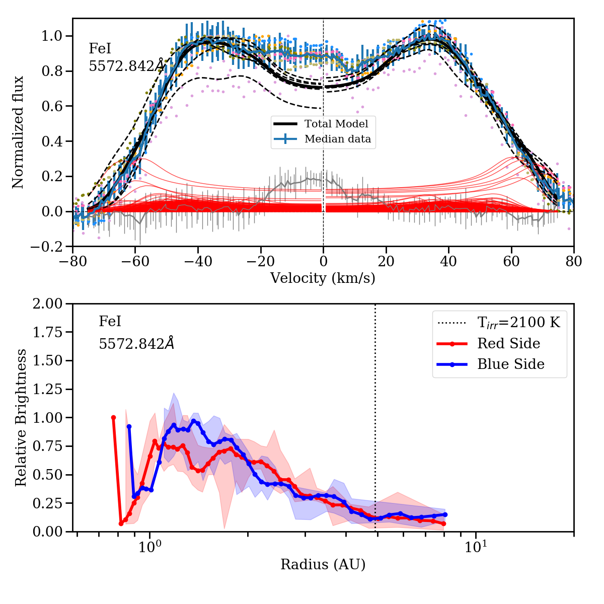
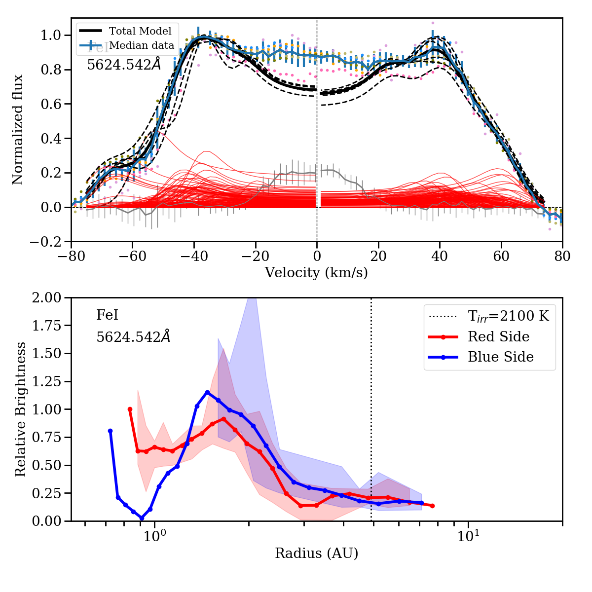
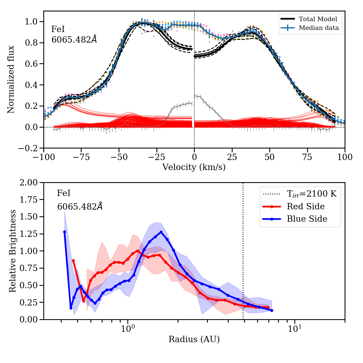
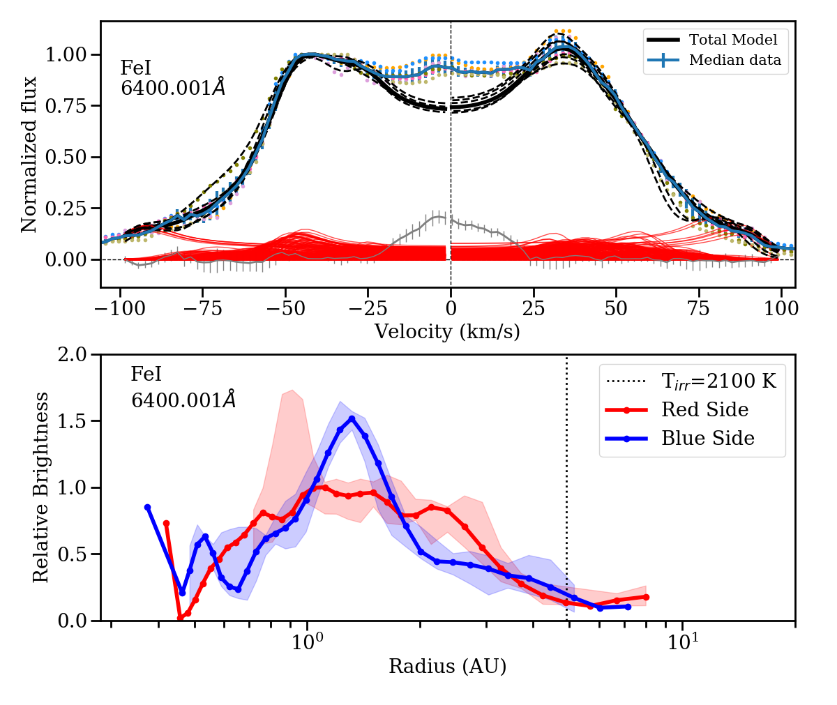
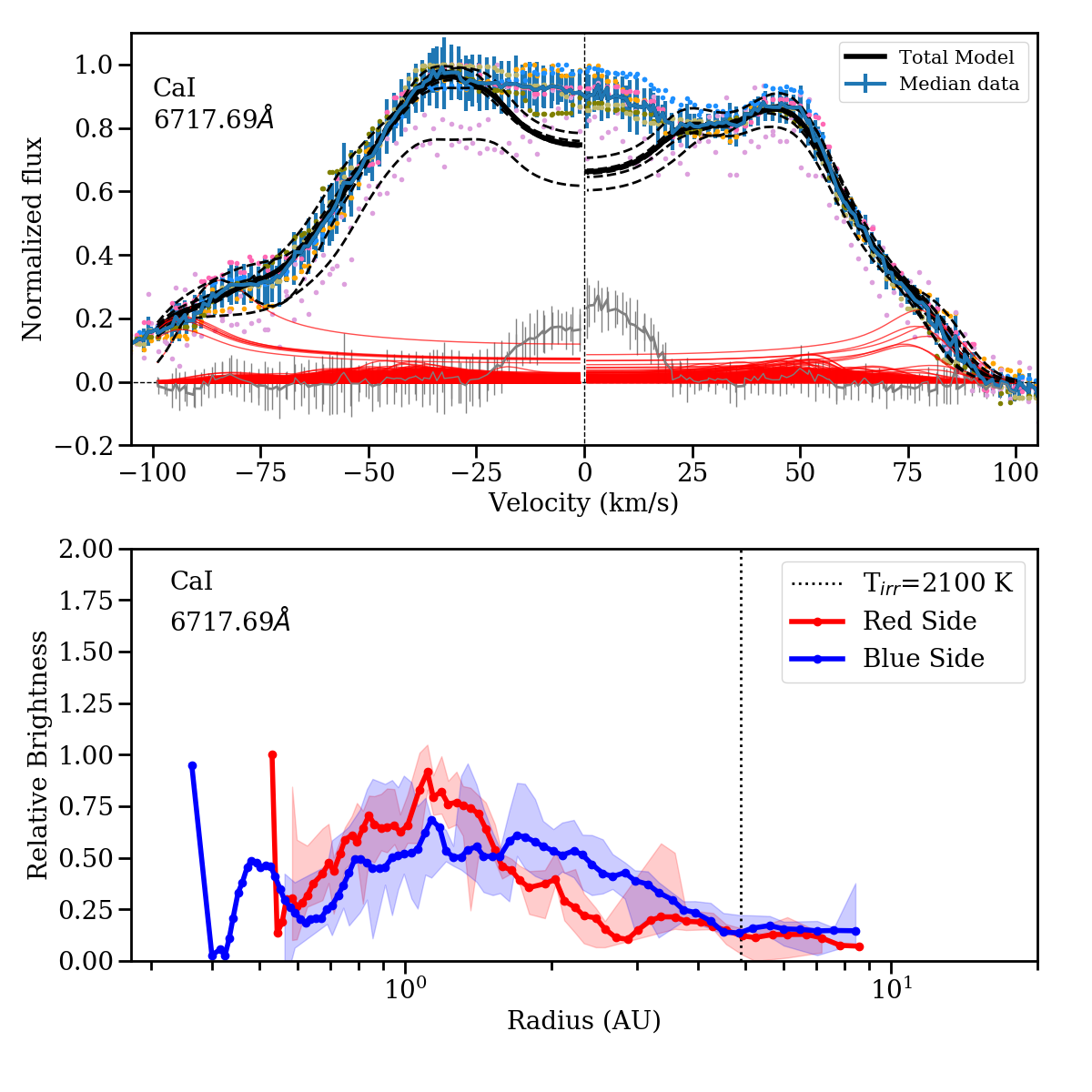
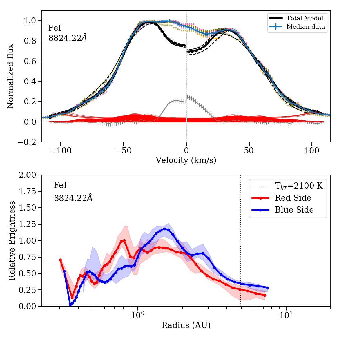
Figure 13: Brightness profile decomposition for the disk-like lines (continued in Appendix C). For each line, the upper panel shows the normalized, median line emission (blue), the individual data points (colored dots), and the model fit. The black solid line is the best fit to the median data, while the dashed lines are the fits to the individual datasets that are used to compute the errors. The zero velocity (measured with respect to the symmetry axis of the line) is shown as a dotted line. The individual ring fits are shown by thin red lines, and the residuals are shown in gray. Since we impose a limit of 35 au to avoid fitting potential narrow emission within the line, the center of the line is not well fitted. In the lower panel for each line, the red and blue thick lines show the best fit to the median spectrum for the red and the blue sides, while the shaded areas show the range spanned by the fits to the individual spectra. Since the noise in the single spectra is higher than in the median spectrum, there are no significant results at extreme velocities for some of the individual datasets. The vertical dotted line indicates the place where direct irradiation results in a temperature of 2100 K, which is independent on the model assumptions and stellar mass. All models are calculated for an inclination of 30 degrees and a stellar mass of 16 M_⊙. A different inclination $i$ would change the derived radii by sin${}^{2}i$/sin${}^{2}(30)$, and a different stellar mass M_∗ would change them by a factor of M_∗/16M_⊙, but the relative brightnesses would remain the same.

Besides the difference in line profile with the transition probability (weak lines look more disk-like than strong ones), there are no significant correlations between excitation potentials, A_ki, and the brightness decomposition. Correlations between the velocity, the full width at half maximum (FWHM) or the peak-to-peak distance, and the atomic parameters are uncertain and noise-dominated. Part of the noise may be caused by the larger variability observed in the line wings of the strong lines that affect their FWHM. Leaving aside the changes that could be attributed to depth and inclination described before, this homogeneity could be a sign that the emitting region is very well constrained and ring-like (Hein Bertelsen et al., 2016).

To summarize, this section confirms the previous results of neutral lines in an irradiated disk-like structure, extending between 0.5-3$\times$(M_∗/16M_⊙) au, and presenting some asymmetries in the surface and the disk midplane as well as radial and azimuthal variations. The double-peaked lines arise from very large radii compared to the stellar radius (and to any reasonable value of the stellar magnetosphere or boundary layer), so these lines cannot provide much information on the accretion mechanism. The temperature ranges inferred from the disk-like lines in the previous sections are not too different from those observed in FUors (i.e., similar to photospheres of F- or G-type stars Hartmann & Kenyon, 1996), although this could result from Fe I emission being strongly suppressed at much higher temperatures. Observations of line profiles in the UV during an outburst would be needed to obtain information on the innermost zones around the star and its temperature and velocity structure. As observed in FUors (Hartmann & Kenyon, 1996), we also see that the lines at longer wavelengths are less disk-like. This could respond to the same effect observed in FUors where lower temperatures, corresponding to further away distances in the disk, have different line profiles. In this respect, it would be useful to check the profiles of near-IR lines, but unfortunately the available near-IR spectroscopy does not resolve the line profiles of neutral atomic lines (Bonnefoy et al., 2017).

3.6 Return to quiescence

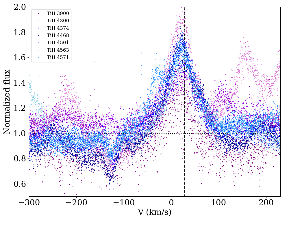
Figure 14: Line profiles of the strong Ti II as observed in quiescence. The data for the various dates are all plotted together, given that there is no significant variability. The vertical line indicates the 27 km s^-1 radial velocity, and the dotted horizontal line indicates the continuum level.

Z CMa NW in quiescence may not be much brighter than its companion, so the three quiescence spectra may contain a combination of Z CMa SE (likely no longer in outburst; Appendix A) and the quiescent Z CMa NW. In the quiescence spectra, the number of emission lines is still high despite being lower than in outburst, but the line profiles are dominated by redshifted emission components instead of blueshifted absorption. The lines are weaker, but due to the changes in the continuum and in the wind absorption, equivalent widths tend to be higher in quiescence. There is no significant variability in the quiescence data (see Figure 15, the apparent variability in faint atomic lines is at the noise level). This could be due to the short time baseline (2009-10-16 to 2009-10-19), but since the outburst spectra show variations on consecutive days, the rapid variations observed in outburst clearly subsided in quiescence.

Outburst	Quiescence	Outburst	Quiescence

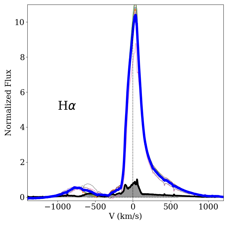
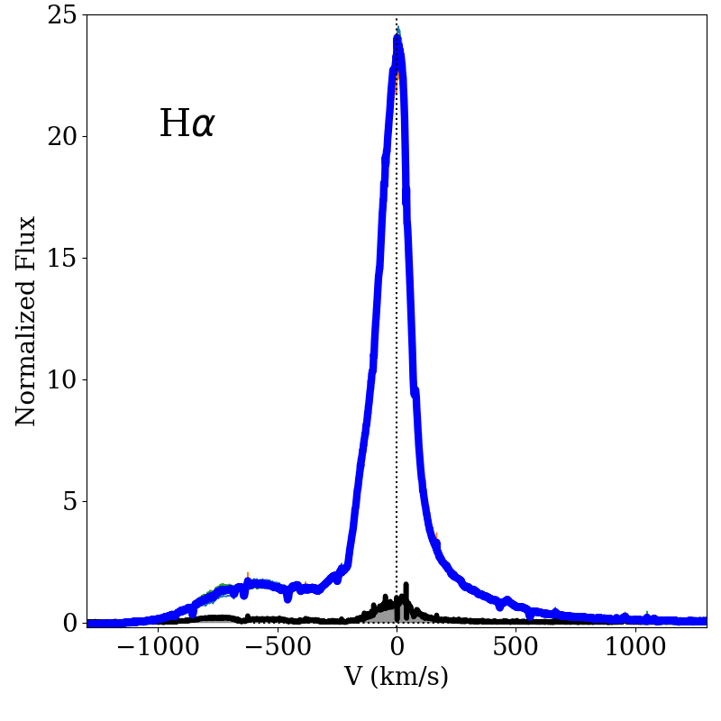
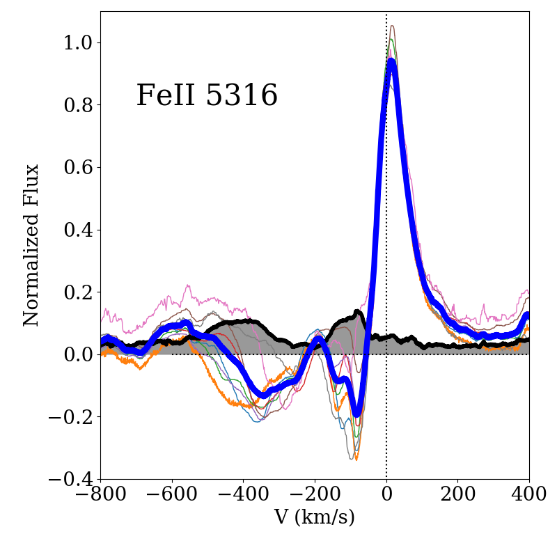
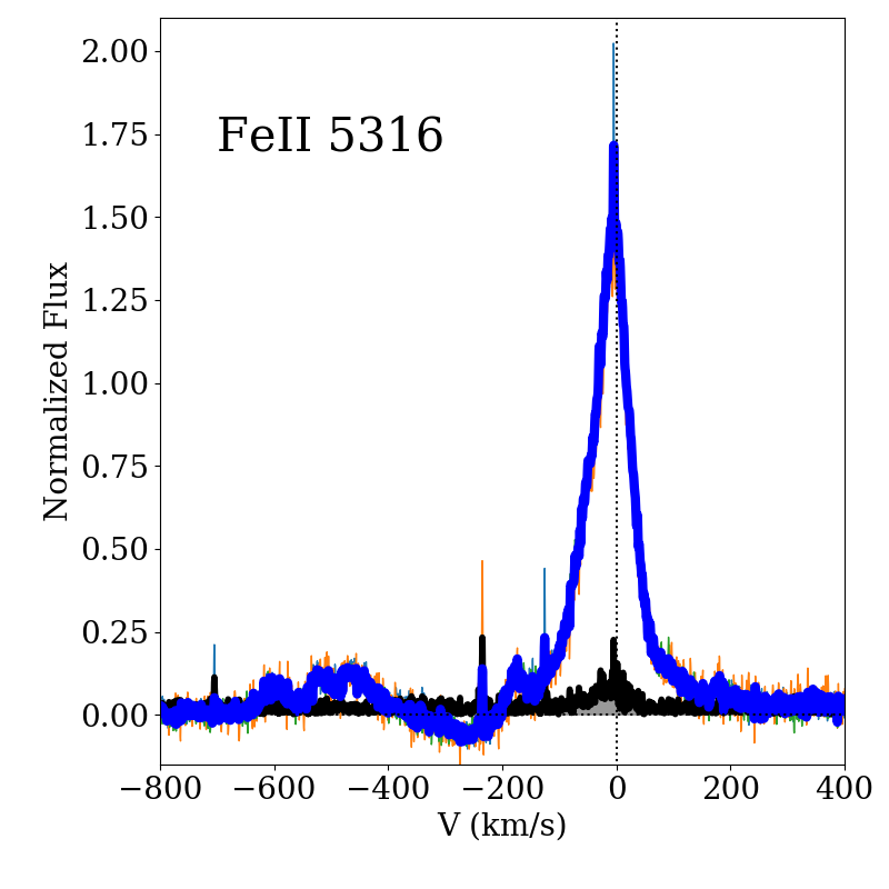
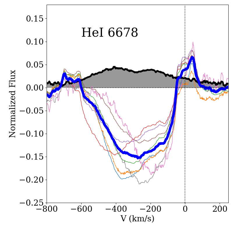
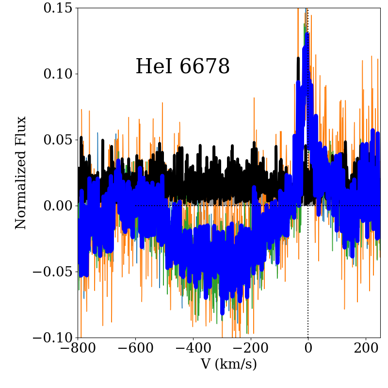
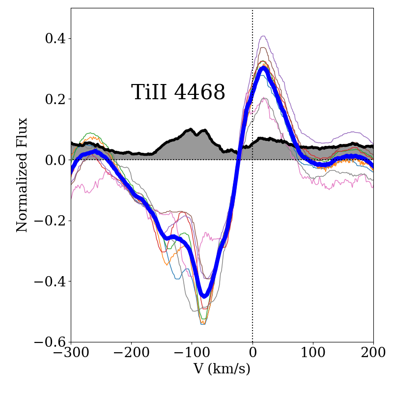
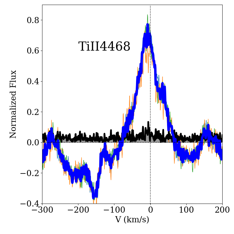
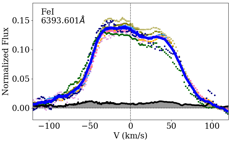
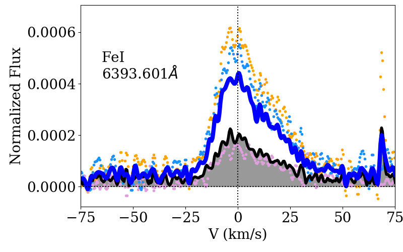
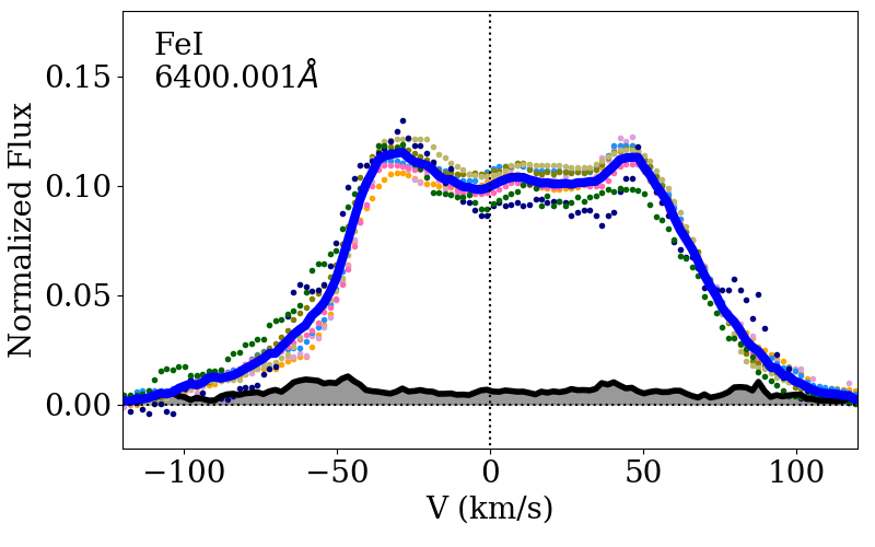
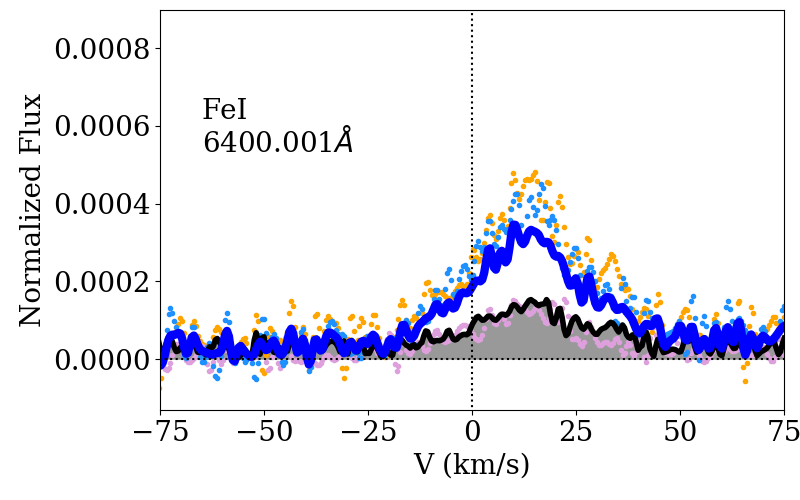
Figure 15: Comparison of the variability observed in several lines in outburst and quiescence. The average flux is plotted in blue, while the standard deviation is shown in black with grey shadowing. The zero velocity (dotted vertical line) is given with respect to the stellar radial velocity. Note: the Fe I 6400Å line in quiescence may contain some contribution of a nearby forbidden [Fe I] line.

The maximum velocity observed in the H$\alpha$ red wing decreases from $\sim$1000 km s^-1 in outburst to $\sim$750 km s^-1 in quiescence, and the wind components faster than -400 km s^-1 are absent from the metallic lines in quiescence. High-energy lines such as Si II are absent in quiescence, and in the He I lines the emission component is stronger and the absorption features are shallower in quiescence (Figure 2). The wind during the quiescence stage is not as clumpy as in outburst, but dominated by a single, more symmetric, wind component instead of several non-axisymmetric components. The intermediate-velocity wind (v${}_{wind}>-$100$/$-200 km s^-1) is still observed in the metallic (including Fe II and Ti II), H I, and He I lines in quiescence, but the strong slow wind (v${}_{wind}\sim-$50$/-$100 km s^-1) disappears in quiescence (Figure 2). This is not unreasonable if the slow wind originates in the disk and the amount of matter transported through the disk decreases in quiescence, affecting the wind mass and optical depth, as often found in accretion-driven outbursts. The low-excitation material also becomes less optically thick during quiescence, which causes most of the weak lines to become very faint or disappear altogether (see Figure 9). The pair Fe I 5624/5572 Å is too weak in quiescence to provide physical results, leaving the temperature largely unconstrained (Figure 12). Optically thinner circumstellar material in quiescence suggests that the disk accretion rate has substantially decreased after the accretion burst, as has also been observed in CO lines in other outbursting stars (Banzatti & Pontoppidan, 2015).

The decrease in optical thickness and column density-velocity gradient in quiescence reveals that, even if the quiescence lines were dominated by the FUor component, the structures accreting onto the FUor are significantly less dense than those of the outbursting Z CMa NW. Differences in inclination may change the observed line widths and depths, but unless accretion covers a significantly larger fraction of the FUor, the accretion rate of the FUor inferred from the densities would be lower, by a couple of orders of magnitude, than the estimated value of 10^-4M_⊙yr^-1 for Z CMa NW in outburst. Since 10^-4-10^-5M_⊙yr^-1 is a typical accretion rate for a FUor (Hartmann & Kenyon, 1996), this is an additional sign that, as of 2009, Z CMa SE had returned to quiescence, although it could be still a strong accretor. We also checked for further signatures of redshifted absorption, characteristic of nonspherical infall or magnetospheric accretion, in the less-blended strong Ti II lines observed in quiescence (Figure 14). The asymmetric redshifted side of the line is suggestive of redshifted absorption, but no consistent trend is observed and the main signature of the Ti II quiescence lines is a strong, narrow wind component at $-$130 km s^-1.

The [O I] components at $\sim$0 km s^-1 and $\sim-$400 km s^-1 seem stronger in quiescence due to the lower continuum levels, but their velocities do not change between quiescence and outburst (see Figure 3). The high-velocity component becomes visible in [S II] in quiescence. The profiles, which are only clearly resolved in quiescence due to contrast, are typical of Herbig-Haro objects. The high-velocity, forbidden line components could be related to the main wind ($\sim-$400 km s^-1) and could correspond to a shock in the wind emission. The second, at $\sim$ 0 km s^-1, could be related to a shock along the disk or extended envelope, but the origin is uncertain since Z CMa SE also drives shocks (Bonnefoy et al., 2017).

Many the low-excitation lines with box- or disk-like profiles in outburst are detected in quiescence, but they are narrow and do not have double-peaked profiles. Since in quiescence the irradiated disk temperature is expected to decrease rapidly, we would expect the disk emission to move to faster velocities as the disk cools down, but the emitting area (and thus the line strength) would also decrease rapidly. Strong neutral lines are often still strong and have complex profiles, suggesting collisional de-excitation in a still-high-density environment. Some of the strongest Fe I lines have asymmetric profiles (e.g., Fe I 6191 and 6393Å lines in Figure 9), dominated by blueshifted emission. This redshifted asymmetry could be indicative of infall or nonspherical accretion, although the velocities are very low ($\sim-$ 20 km s^-1). The typical FWHM of 20-30 km s^-1 for the metallic quiescence lines would correspond to Keplerian rotation at $\sim$16$\times$(M_∗/16M_⊙) au, at which the disk will be too cold in quiescence. Their wings extend out to $\pm$50 km s^-1 and could be related to the innermost disk (3-5$\times$(M_∗/16M_⊙) au), but line width is very small compared to infall or rotation velocities around an intermediate-mass star. The lower luminosity in quiescence suggests line formation closer to the star. If the lines were associated with small and localized hot spots on the stellar surface, we would expect to see some rotational modulation, unless the star is seen close to pole-on. The lack of rotational modulation in the narrow quiescence emission lines suggests that the material is either at a polar, always-visible spot, or extended in a rather uniform way around the star. This could be expected for unstable accretion (Kurosawa & Romanova, 2013) or if the star accreted through an axisymmetric structure or boundary layer. Stellar rotation could account for the line broadening if the star is a slow or highly inclined rotator. Further observations over a more extended period of time would be needed to clarify this issue and, in particular, to determine the longer-term variability during quiescence that may betray its spatial location. Summarizing, quiescence brings a dramatic decrease of mass accretion and wind density, triggering the disappearance of the low-velocity disk wind and non-axisymmetric wind components.

4 Outbursts in high-mass versus low-mass stars

One of the most surprising results of our analysis is that the spectral behavior of Z CMa NW in outburst and quiescence is qualitatively not too different from what has been observed in other EXors (Herbig, 2007, 2008; Sicilia-Aguilar et al., 2012, 2017; Holoien et al., 2014; Audard et al., 2014). From historical photometric evidence (see Appendix A), the outbursts of Z CMa NW are not different from the outbursts of lower-mass EXors, repeating in time every few years and showing various patterns in time duration and intensity (Herbig et al., 2001; Herbig, 2007; Audard et al., 2014). In both EX Lupi and Z CMa NW, the accretion-related wind becomes stronger during outburst, and the line wings of essentially all lines move toward greater (positive and negative) velocities. Emission originating from the inner disk is also detected in both objects, although in EX Lupi the emitting material within the inner disk is highly non-axisymmetric (e.g., a single accretion column or disk spiral) and very close-in, which results in dramatic day-to-day velocity variations in the broad components of the lines (Sicilia-Aguilar et al., 2012). Non-axisymmetric winds have also been observed in the M5 star ASASSN-13db during outburst (Sicilia-Aguilar et al., 2017). Evidence of changes in the inner disk content after bursts has been documented in EX Lupi (Banzatti & Pontoppidan, 2015), which is consistent with the decrease in optical thickness in the line-emitting region observed for Z CMa NW after outburst. The larger luminosity of this outburst agrees with the idea of a continuum of bursting stars, not only in the magnitude of the burst (Contreras Peña et al., 2017), but also in stellar mass.

The emission lines observed in Z CMa NW, EX Lupi, and ASASSN-13db have statistically indistinguishable distribution of transition probabilities. The only significant difference arises between the excitation potentials of the lines observed in Z CMa during outburst and ASASSN-13db, thus rejecting at the 1% level the hypothesis that both samples are drawn from the same distribution, according to a double-sided Kolmogorov-Smirnov test. This difference in excitation potentials likely results from the large difference in stellar temperature (B-type vs. M5). The similarities point to a rather uniform range of physical conditions for the material in the inner disk and accretion structures. However, because of the differences in the masses and effective temperatures of the three stars, the regions in which this emission originates ranges from a few stellar radii for ASASSN-13db (Sicilia-Aguilar et al., 2017), to 0.1-0.2 au for EX Lupi (Sicilia-Aguilar et al., 2012), and to 0.5-3$\times$(M_∗/16M_⊙) au for Z CMa NW.

The accretion scenario for Z CMa NW can be also explored through its emission and absorption lines. Although contributions from different origins (e.g., nonspherical winds) may affect the extremely redshifted H$\alpha$ wings, there are some small redshifted absorption asymmetries in the Ti II and Fe I lines (in the range of 50-150 km s^-1) and in the high-velocity wings of accretion-related lines. These asymmetries are mainly observed during outburst in the higher Balmer lines and in H IR lines (see Figure 2, small absorption components appear at $\sim$+200 and +400 km s^-1 in H$\beta$ and $\sim$250 km s^-1 in H$\gamma$). These could indicate a high-velocity infall scenario (e.g., Koenigl, 1991; Edwards et al., 1994; Muzerolle et al., 1998) rather than a classical boundary layer, where the velocities in the boundary would be much reduced (e.g., Popham et al., 1993). Nonetheless, these velocities suggest a stellar mass much lower than 16 M_⊙, even if the magnetosphere was very small. Using as the maximum infall velocity that observed in the the H$\alpha$ line wings (1000 km s^-1) this would result in a 2.7 R_∗ or 5.2 R_⊙, which is on the small side for magnetospheric accretion in intermediate-mass stars (e.g., Mendigutía et al., 2017), albeit not unexpected in a fast-rotating star with a weak magnetic field. A variation in stellar mass by a factor of two would bring the infall radius to the classical infall radius for a low-mass stars (Gullbring et al., 1998).

Nevertheless, the corresponding field to ensure a magnetospheric cavity extending as far as the corotation radius for R_cor=2.5 R_∗ would be on the upper limit for HAeBe stars. The minimum magnetic field $B_{min}$ required to support magnetospheric accretion can be estimated as

$$B_{min}=1.1\bigg{(}\frac{M_{*}}{M_{\odot}}\bigg{)}^{2/3}\bigg{(}\frac{\dot{M}}{10^{-7}M_{\odot}/yr}\bigg{)}^{23/40}\bigg{(}\frac{R_{*}}{R_{\odot}}\bigg{)}^{-3}\bigg{(}\frac{P}{1d}\bigg{)}^{29/24}\text{kG}$$ (7)

(see Collier Cameron & Campbell, 1993; Johns-Krull et al., 1999; Mendigutía, 2020) as a function of the rotational period of the star, P, which is a priori not known. A corotation radius of 2$\times$R_∗ requires a stellar rotation period of 0.22 d (for a 16 M_⊙ star), down to 0.44 d (for a 4 M_⊙ star), but the minimum magnetic field needed to support the accretion rate observed in outburst via magnetospheric accretion would be at least 8 kG and up to 16 kG for a 4 M_⊙ star, since a lower stellar mass also means a higher accretion rate for the same accretion luminosity. This is much larger than the existing estimates for the Z CMa pair (1.2 kG; Szeifert et al., 2010; Hubrig et al., 2015) and the typical fields of HAeBe stars. On the other hand, assuming that in quiescence the accretion rate drops to the typical HAeBe rate of 10^-7M_⊙/yr, a magnetic field of 0.2 kG would be able to support magnetospheric accretion for a 16 M_⊙ star, and a lower-mass star would require a weaker field.

A more detailed estimate of the equatorial magnetic field required could be derived following (Bessolaz et al., 2008)

$$B_{*}= 140\times 2^{-7/4}m_{s}^{-1/2}\bigg{(}\frac{R_{t}}{R_{*}}\bigg{)}^{7/4}\bigg{(}\frac{\dot{M}}{10^{-8}M_{\odot}/yr}\bigg{)}^{1./2.}\bigg{(}\frac{M_{*}}{0.8M_{\odot}}\bigg{)}^{1/4}$$ (8)

$$\bigg{(}\frac{R_{*}}{2R_{\odot}}\bigg{)}^{-5/4}G,$$

where $R_{t}$ is the truncation radius, $m_{s}$ is the Mach number ($\sim$0.45; Bessolaz et al., 2008), and the rest of symbols retain their previous meaning. This approach results in an even higher magnetic field during outburst (46-65 kG) for a star with a mass between 4-16 M_⊙, which is completely unfeasible. The result for the quiescence accretion rate of 1e-7 M_⊙/yr would range from 1-1.5 kG for stars with masses between 4-16 M_⊙, which although feasible for the more magnetic HAeBe stars, remains questionable until such a high magnetic field has been confirmed. Therefore, although magnetospheric accretion is highly unlikely in outburst, which would be a significant difference compared to lower-mass EXors, it may be possible in quiescence.

5 Summary and conclusions

We present optical spectroscopy during the outburst and post-outburst phase of Z CMa NW, using the wealth of emission lines observed to explore the causes of the outburst and the properties of the accreting star. We confirm that the outburst of Z CMa NW was related to an increased accretion episode reaching Ṁ$\sim$10^-4 M_⊙ yr^-1. This accretion rate is significantly higher than the current accretion rate of the FUor companion Z CMa SE, for which photometric and spectroscopic evidence suggest a return to quiescence by year 2000. The historical light curve (including AAVSO data since the 1930s) and past spectroscopic activity (e.g., Hessman et al., 1991) suggest that the outbursts of Z CMa NW are repetitive, as in low-mass EXors. We use several techniques, including velocity decomposition to track the spatial location, Saha’s equation and line ratios of lines from the same upper level, to estimate the density and temperature of the various regions, which include a non-axisymmetric, multicomponent wind and extended disk emission.

The optical spectra strongly resemble EXor outburst spectra for lower-mass stars, suggesting a continuum of accreting behaviors for disked stars with all masses. The spectra of Z CMa NW in outburst reveal lines with multiple origins. A double-peaked line emission originates in a hot disk (detected in neutral atomic lines, especially Fe I). Complex wind absorption with several velocity components is most evident in H, He I, and in the higher-energy metallic ionized lines such as Fe II, Si II, and Ti II. There is also some evidence of redshifted asymmetries that could be related to infall or accretion structures, which are detected preferentially in H and single-ionized elements such as Fe II, and Ca II in outburst, and in the asymmetry of neutral lines in quiescence. This is not dissimilar to what is seen in lower-mass stars, although the velocities also suggest that the stellar mass is likely lower than 16 M_⊙. Age and luminosity considerations suggest a value around 6-8 M_⊙.

The magnetosphere - if present - is expected to be very small, and it is highly unlikely that the magnetic field is strong enough to support magnetospheric accretion during outburst, although it may be possible in quiescence if the star belongs to the most magnetic HAeBe stars. This is significantly different from lower-mass EXors, and challenges the role of a magnetosphere in the triggering of some outbursts (e.g., as suggested for EX Lupi; Sicilia-Aguilar et al., 2015). We do not observe a boundary layer in the classical sense either, but rather extended accretion structures. We also observe a more distant Keplerian, irradiated disk. The energetics of the optical emission lines may impose a limitation to the temperature we can reach, and UV lines may be needed to trace such a hotter, closer structure.

The disk emission observed in Fe I and Ca I lines is best fitted with an irradiated, flared disk originating in the inner $\sim$0.5-3$\times$(M_∗/16M_⊙) au regions, which have temperatures in the 2000-7000 K range and densities that decrease toward lower velocities (larger radii). Weak Fe II lines are also consistent with disk emission, although they trace higher temperature regions. For the disk to be dominated by irradiation, it is necessary that the bulk of energy released in the accretion burst is deposited at a small radius (e.g., in the innermost disk, accretion structures, or on stellar hot spots). There is no evidence of the temperature inversion associated with viscous heating in strongly accreting systems, but this could happen if the part of the irradiated disk that we observe in the Fe I lines is too distant from the hot, dense, accretion-powered inner disk. The disk-like features of higher energy and ionized lines from the hotter, innermost regions in the disk may be masked by the strong emission and absorption profiles produced by the hot stellar wind. We observe a decrease in column density-velocity gradient per velocity bin, and for the redshifted components of the lines, decreases by at least one order of magnitude between outburst and quiescence, a sign of a lower mass transport through the disk.

The blueshifted absorption features are consistent with an accretion-powered wind. The fastest and slowest wind components disappear in quiescence, when the wind density decreases. The temperature in the fast wind is higher than in the slow wind, betraying an origin very close to the star, while the slow component could be a disk wind. The changes in velocity and depth of the absorption are consistent with a clumpy, non-axisymmetric wind with spatially variable opacity, modulated by rotation. This is similar to the winding winds observed in B-type stars (Prinja, & Howarth, 1988), but the behavior disappears in quiescence and thus is linked to the outburst rather than to the spectral type. Our small number of observations does not allow us to determine whether the velocity changes display any periodicity, but the presence of a non-axisymmetric wind is an additional sign that accretion is non-axisymmetric as well.

This study, together with our previous work on low-mass stars (Sicilia-Aguilar et al., 2012, 2015, 2017), demonstrates that optical spectroscopy can be used to trace the structure, radial distance, and physical conditions of accretion in stars with a large range of mass. Combined with historical data, it shows that a similar outbursting behavior can be observed through a very large range of stellar masses and spectral types (from M5 to B-type), pointing to common outburst mechanisms and similarities in accretion and inner disk transport within this whole range, despite potential differences in the structure and size of the magnetosphere. The limited energy ranges covered by the lines that can be observed in optical spectra also point out the need for high-resolution UV and IR spectroscopy data to study the full energetic range of this kind of objects.

Acknowledgments: We thank Steve Shore, Lynne Hillenbrand, Andrew Collier Cameron, Lee Hartmann, Peter Woitke, and Ignacio Mendigutía for inspiring discussion, as well as the anonymous referee for valuable comments. ASA is partly supported by the STFC grant number ST/S000399/1 (”The Planet-Disk Connection: Accretion, Disk Structure, and Planet Formation”) and by the 2017 Visiting Teacher Campaign at the University of Grenoble. We thank the former OHP Director, Michel Boer, for granting discretionary time to perform these observations. We thank Anne Eggenberger for performing the second set of spectroscopic observations at OHP during quiescence. This project has received funding from the European Research Council (ERC) under the European Union’s Horizon 2020 research and innovation programme (grant agreement No 742095; SPIDI: Star-Planets-Inner Disk-Interactions”, http://spidi-eu.org, and grant agreement No 740651 NewWorlds). We acknowledge with thanks the variable star observations from the AAVSO International Database contributed by observers worldwide and used in this research, and in particular, observers from the Royal Astronomical Society of New Zealand (RASNZ).

Appendix A Variability: 90 years of photometric data

The AAVSO contains data on Z CMa since the 1930s. These data provide a great opportunity to examine the behavior of the Z CMa pair over nearly 90 years. The AAVSO confirms that the light curve is anomalous compared to other FUors (Hartmann et al., 1989; Hessman et al., 1991), since the documented magnitude rise spans only 2 mags and seem to have progressed very slowly for the first 30 years. The light curves are shown in Figure 16, suggesting that the FUor outburst probably ended by 1995. Since then, the outbursts of Z CMa NW have been recurrent and increasing in brightness, although both the AAVSO data and early mentions of small-scale variability over the FUor curve (Hessman et al., 1991) suggest that the outbursts may have been occurring at least since the early 1980s, masked in part by the FUor outburst of the companion. Thus the P Cygni profiles observed to dominate the spectrum during bumps (Hessman et al., 1991) may have been caused by the HBe star, and not by its FUor companion. In any case, the bursts appear to have increased in intensity since the 2000s, and deserve some future follow-up.

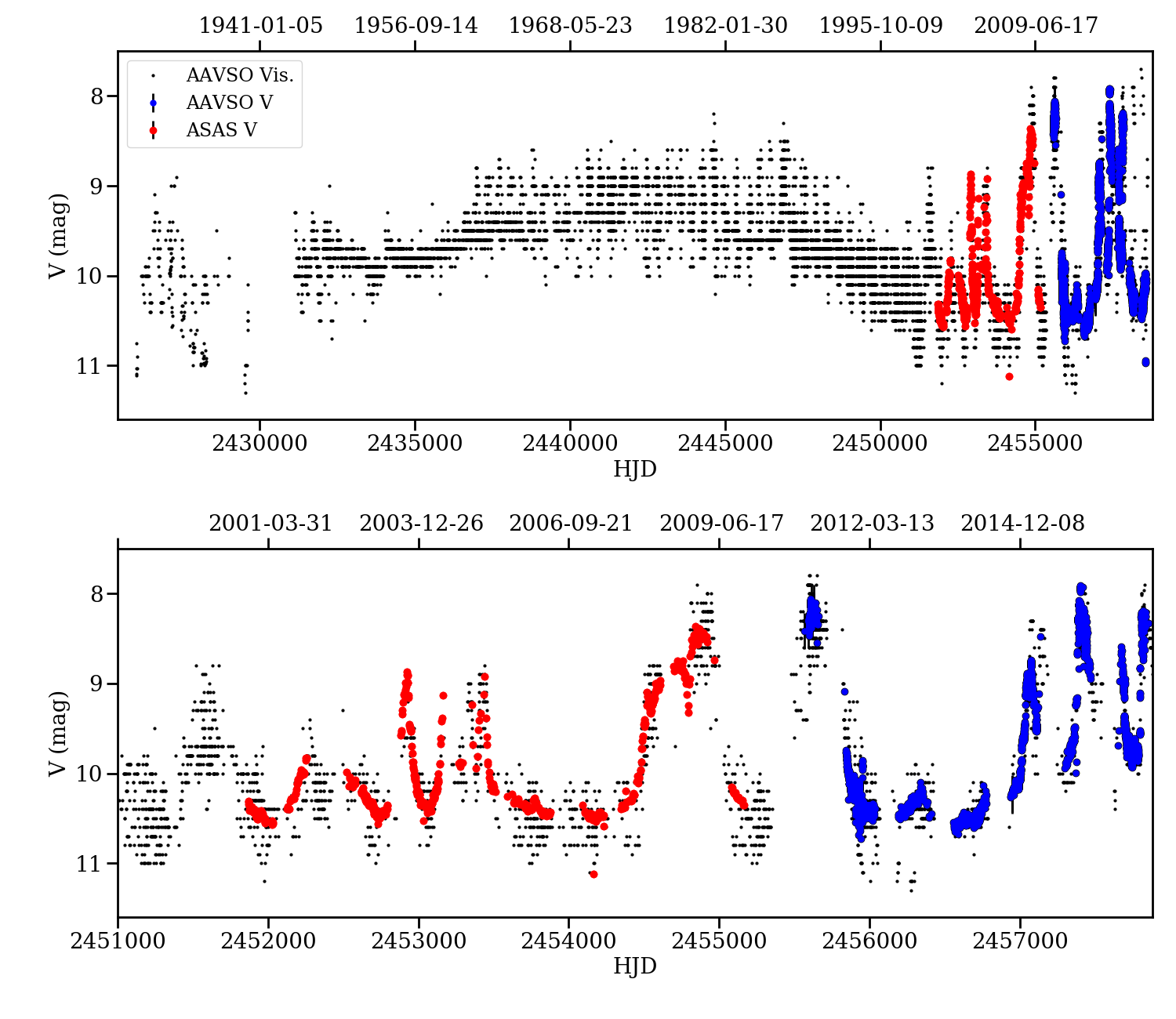
Figure 16: Light curves from AAVSO for Z CMa since 1930s (upper) and from 1999 to 2018 (lower). Only verified observations are included. The visual and V filters are plotted together, since they are similar for the current purpose of examining the timescales of the outbursts. As a comparison, the ASAS V filter is also plotted (red), which is in excellent agreement with the amateur V data.

A generalized Lomb-Scargle periodogram (GLSP; Scargle, 1982; Horne & Baliunas, 1986; Zechmeister, & Kürster, 2009) reveals a low-significance quasi-period of 249$\pm$20 d (Figure 17) when the ASAS and AAVSO V data (covering 14 years) are taken into account. The modulation appears to change in phase, which suggests a quasi-periodic behavior in a component that changes at about the same rate as the periodicity is observed. Using a red noise model (as done in Sicilia-Aguilar et al., 2020), the false-alarm-probability of the modulation is $\sim$1%. Although this potential period needs to be confirmed in the coming years, it could be related to repeated disturbances in the innermost disk causing the bursts.

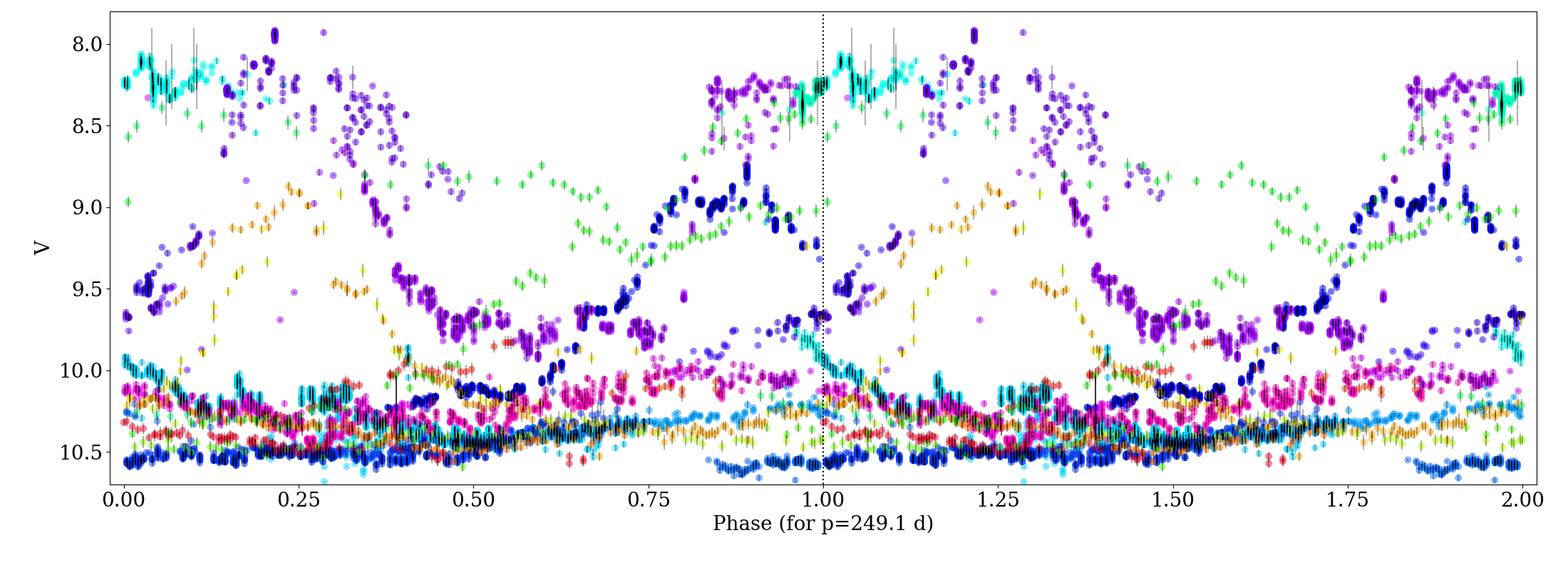
Figure 17: Data from ASAS and AAVSO V wrapped according to a 249.1 d period. The data are colored depending on the epoch to enable visualization.

As seen in Figure 1, the two first spectra were taken as the star emerged from an occultation-like event, in which the rising magnitude experienced a drop of more than 0.5 magnitudes and then recovered; the whole event lasted about 30 days. Unfortunately, the spectra were taken when the star had nearly recovered, so any occultation effects may be mild. These two first datasets also seem to show distinct wind features, such as a less complex profile more similar to the quiescence profile. This could be caused by either a larger contribution of the FUor spectrum if Z CMa NW is partly occulted or suggest that part of the wind-originating location could have been occulted by the material that caused the observed dip. The high temperatures inferred for the fast wind are consistent with an origin closer to the star, which would be also easier to be hidden by an occultation event than, for instance, a more extended disk wind. The effect is mostly observed in Fe II lines (5018, 4923, 4233 Å), which are also some of the most variable lines among those with P Cygni profiles. Nevertheless, since the first spectrum has stronger wind absorption than the second spectrum, the wind is by itself very variable and these observations were taken about a month before the following observations, what we observe in the wind may be just part of the usual wind variability unrelated to the occultation event. Figure 1 reveals that similar dips during previous outbursts of Z CMa NW have occurred. They are more evident during the last ten years, after the FUor outburst had dimmed and during the time when the activity of Z CMa NW seems to have increased, and could be related to variable extinction suggested by Blondel & Djie (2006). Future follow-up may help to understand the origin of the dips and to locate the occulting material and the regions it affects.

Appendix B Complete list of emission lines

The line identification was done using the NIST database, except for lines denoted with WS, for which the line identification and atomic parameters have been taken from Wahlgren & Shore (S. Shore, private communication) and their observations of the symbiotic star V407 Cyg outburst. We compare the observed lines with the lists of van den Ancker et al. (2004) from observations of Z CMa between the late 1990s and the early 2000s (including weaker outbursts) and the lines observed in two outbursting stars, EX Lupi (Sicilia-Aguilar et al., 2012, 2015) and ASASSN-13db (Sicilia-Aguilar et al., 2017), for which a similar analysis is published. The observed profiles were also used to classify a line, or at least to identify the dominant component in case of blends or multiple options, when more than one transition was possible. As mentioned in the text, strong Fe II lines (and also Cr II and Si II lines) have P Cygni profiles. Weak Fe II lines with low transition probabilities are similar to Fe I lines. A few forbidden lines are also observed; [O I] 6300/6363Å is the strongest, followed by [S II]. Some redshifted outflow emission could be present, but blends make this possibility uncertain at best. Some [Fe II] lines are detected, but they tend to be very weak and, in most cases, they appear blended with or very close to other very strong lines so that their profiles are hard to compare and the detections remain tentative. Some of the [Fe II] lines may also be observed in quiescence.

Appendix C Methodology

This appendix contains the details of the different methods used to analyze the emission and absorption lines that are applied in Section 3.

C.1 Deriving physical properties from the spectral lines

To constrain the physical conditions of lines originating from the same location, we compared the strength of the ionized and neutral lines to put constraints on the density and temperature using Saha’s equation,

$$\frac{n_{j+1}n_{e}}{n_{j}}=\bigg{(}\frac{2\pi m_{e}kT}{h^{2}}\bigg{)}^{3/2}\frac{2U_{j+1}(T)}{U_{j}(T)}e^{-\chi_{I}/kT},$$ (9)

where $n_{j+1}$ and $n_{j}$ are the densities of the ionized and neutral species, respectively; $\chi_{I}$ is the ionization potential; $n_{e}$ is the electron density; $m_{e}$ is the electron mass; $k$ is the Boltzmann constant; $h$ is the Planck constant; T is the temperature; and $U_{x}(T)$ is the partition function for the x-ionized ion at a temperature T (Mihalas, 1978). The main limitations of this approach are non-LTE effects and optical depth and self-absorption (as observed in EX Lupi, Sicilia-Aguilar et al., 2012). We expect at least some of the lines to be optically thick, which is a problem when using line ratios to derive the physical properties. Nevertheless, the non-detection (or detection) of low-energy lines is a very powerful way to set a limit to the temperature for reasonable densities, or vice versa. For this exercise, we used the atomic parameters and partition functions for different temperatures from the NIST spectral line database (Ralchenko et al., 2010; Kramida et al., 2018) and made sure that the line profiles of the compared transitions are very similar in velocity and line profile, to minimize the risk of including emission produced by different structures.

A further constrain is obtained from the ratio of the transitions of the same ion. As a first approach, if we ignore radiative transfer effects and assume that the lines are optically thin, the levels are populated according to Boltzmann statistics, so that

$$\frac{n_{i}}{n_{0}}=\frac{g_{i}}{g_{0}}e^{-Ei/kT},$$ (10)

where $n_{i}$ and $n_{0}$ are the densities in the levels $i$ and the ground state, respectively; $g_{i}$ and $g_{0}$ are their statistical weights; and $E_{i}$ is the energy of the level with respect to the ground state.

A second calculation can be performed considering the ratio of two lines that share a common upper level. In such a case, the way the upper level is populated does not matter, and the line ratio depends only on the optical thickness of each line (Beristain et al., 1998). If we estimate the ratio of the weakest to the strongest line, the optically thin limit (for which both lines are optically thin) depends on the line properties alone. While the strongest line is saturated, the ratio increases until it reaches a limit once the weakest line is also saturated. In particular, for isotropic high-velocity gradients, we can use the Sobolev approximation to treat the escape probability (Beristain et al., 1998) so that the line ratio can be written as

$$r_{w/s}=\frac{A^{w}_{ki}\lambda_{s}}{A^{s}_{kj}\lambda_{w}}\frac{1-e^{-\tau_{w}}}{\tau_{w}}\frac{\tau_{s}}{1-e^{-\tau_{s}}},$$ (11)

where A_ul is the Einstein coefficient for the spontaneous transition from levels u to l, $\lambda$ is the wavelength, and $\tau$ is the opacity, and the indices $w$ and $s$ mark the weak and the strong line, respectively. The opacity in the Sobolev approximation for the transition between levels k (up) and i (low) can be written as

$$\tau=\frac{hc}{4\pi}\frac{n_{i}B_{ik}-n_{j}B_{ki}}{dv/dl}\approx\frac{hc}{4\pi}B_{ik}g_{i}\frac{e^{-E_{i}/kT}}{U(T)}\frac{ndl}{dv},$$ (12)

where $B_{ik}$ and $B_{ki}$ are the Einstein coefficients for stimulated absorption and emission and the approximation can be obtained by neglecting the population in the upper level and assuming thermal equilibrium (Mihalas, 1978; Beristain et al., 1998). The velocity gradient is written $dv/dl$ and $E_{i}$ is the energy of the lower level. Rearranging Equations 11 and 12, we can write the line ratio in terms of the temperature and modified column density or column density-velocity gradient $\mathcal{N}=ndl/dv$.

Using nearby lines (with wavelengths within a $\leq$500$\AA$ range) is preferred to avoid effects of underlying variable continuum. We note that the main uncertainty related to the atomic parameters comes from the B_ij parameters, thus the main uncertainties lie in the derived line opacities. This exercise was done for several velocity ranges along the line profile (see Section 3.4). Some lines are shown in the main text, with the remaining lines shown in Figures 18 and 19.

Outburst	Quiescence

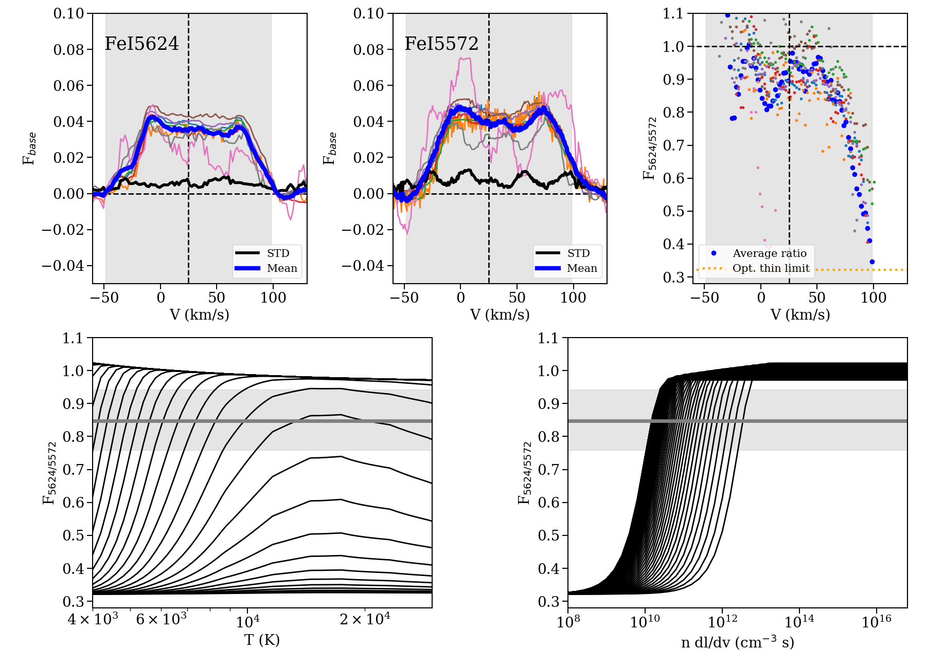
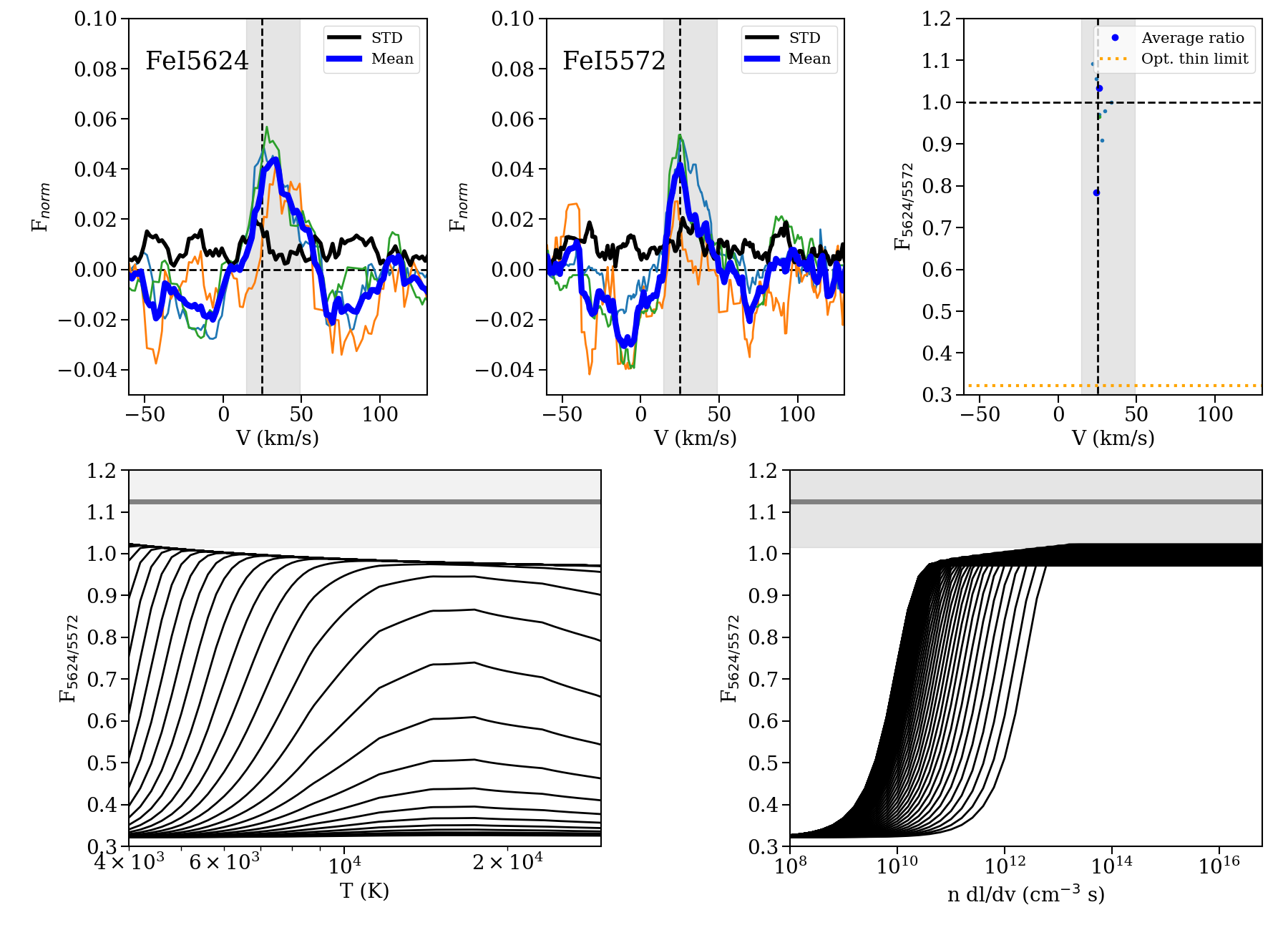
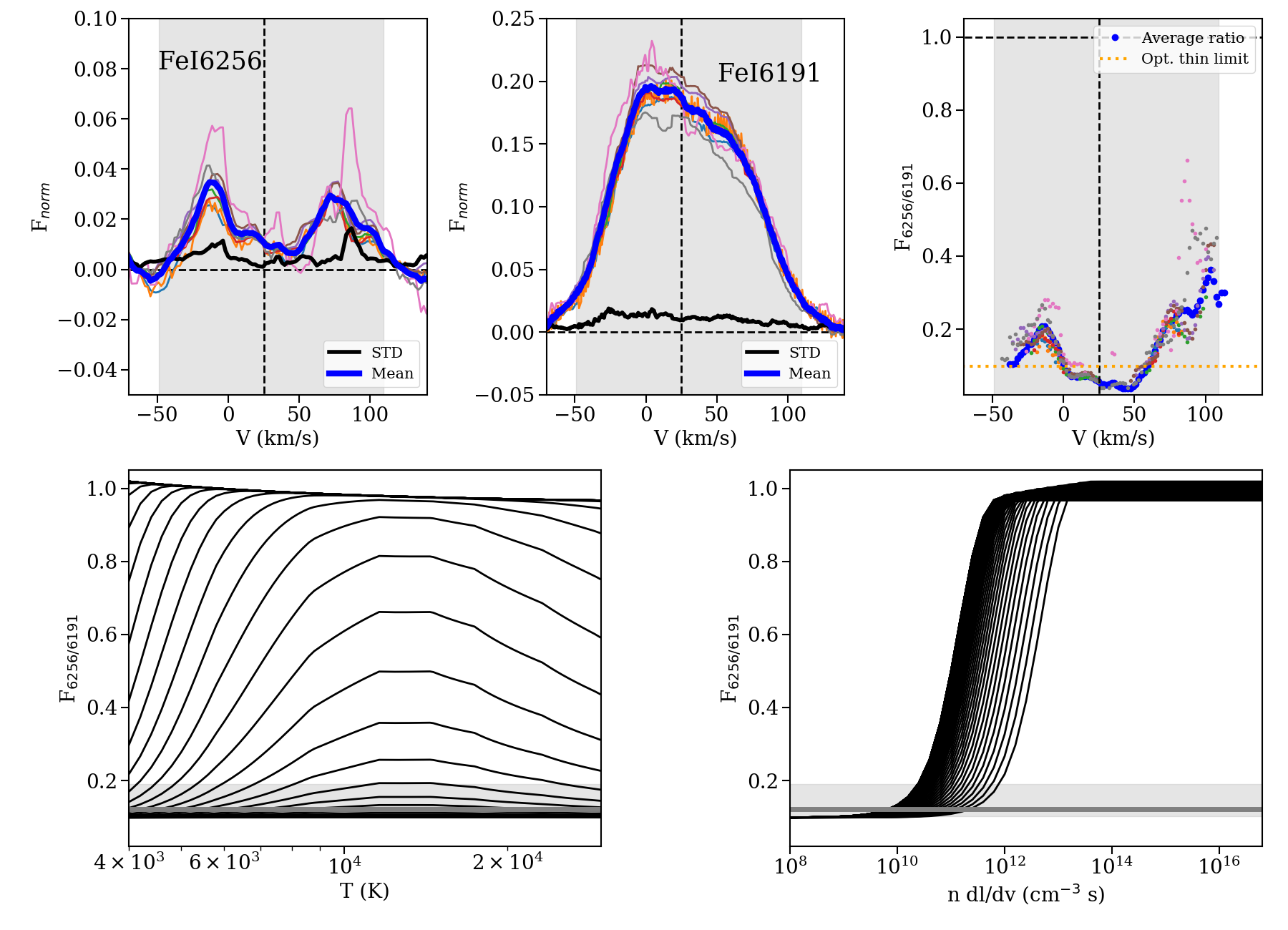
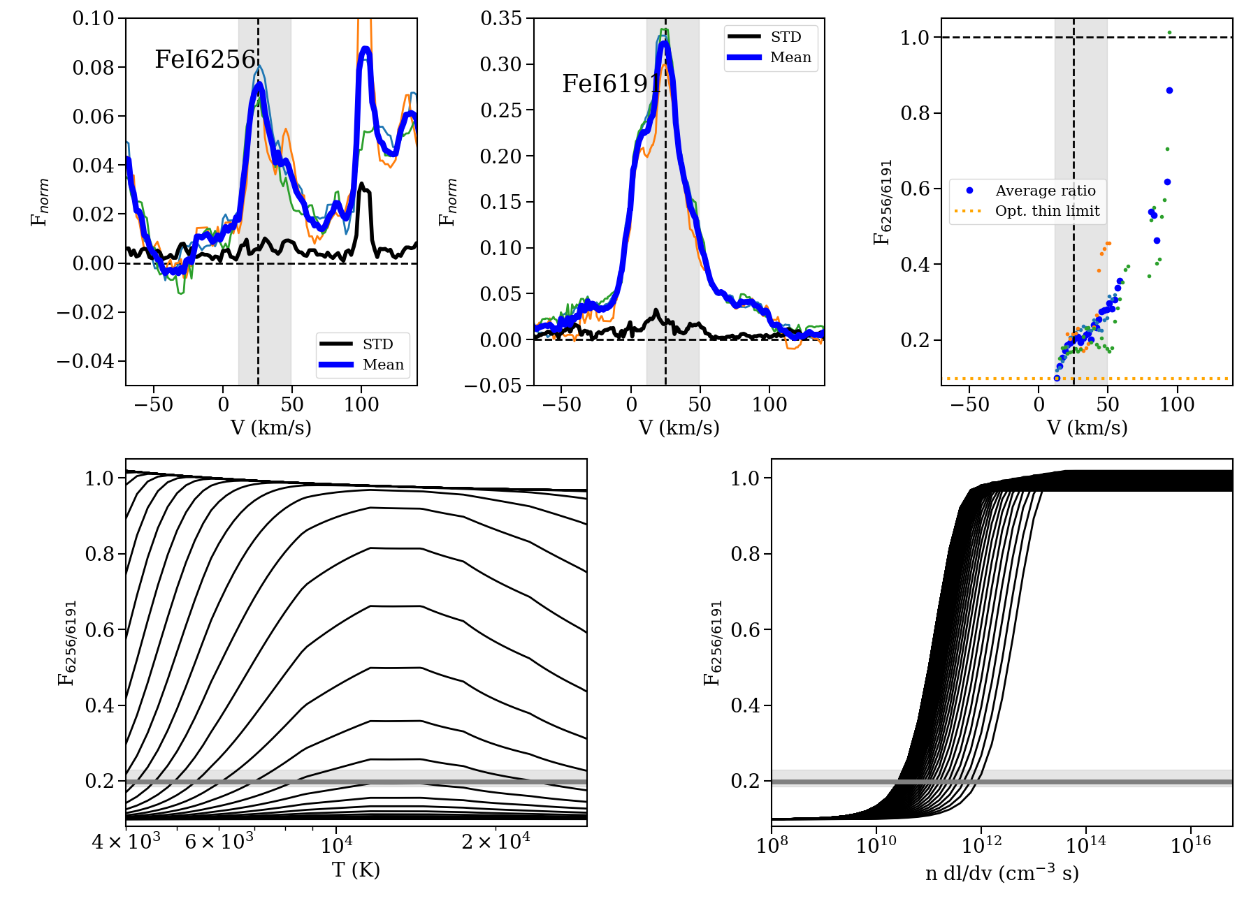
Figure 18: Analysis of the line ratio for Fe I transitions with upper common levels (Figure 9, continued). The upper left panels show the line emission in outburst; the upper right panel shows the quiescence data. The ratios observed are compared to the theoretical calculations for a range of temperatures and column density-velocity gradients in the lower panels. The gray area shows the region for which the line emission is $>$5$\sigma$ (in the velocity panels), and the 1$\sigma$ error in the temperature and density planes.

Outburst	Quiescence

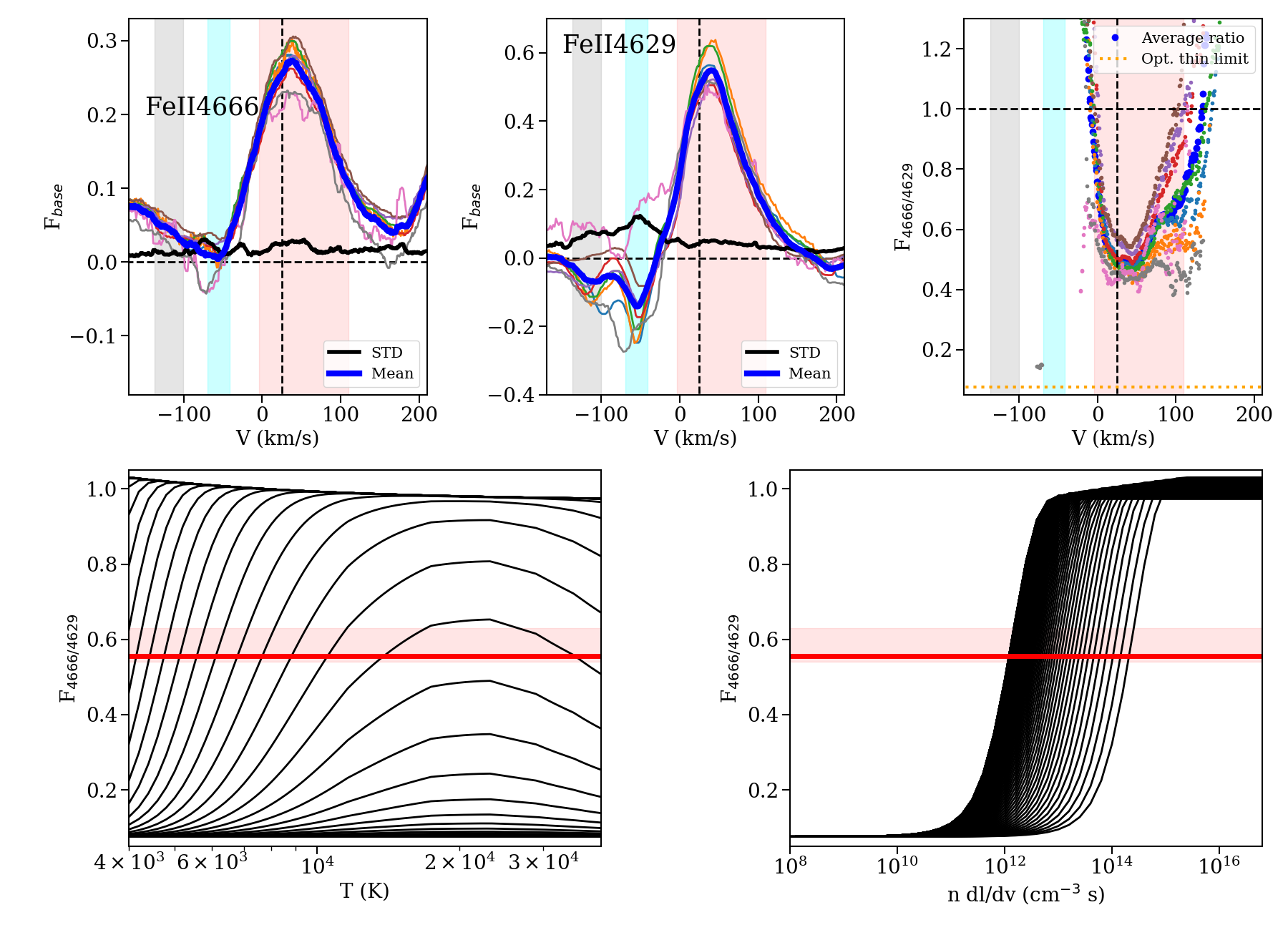
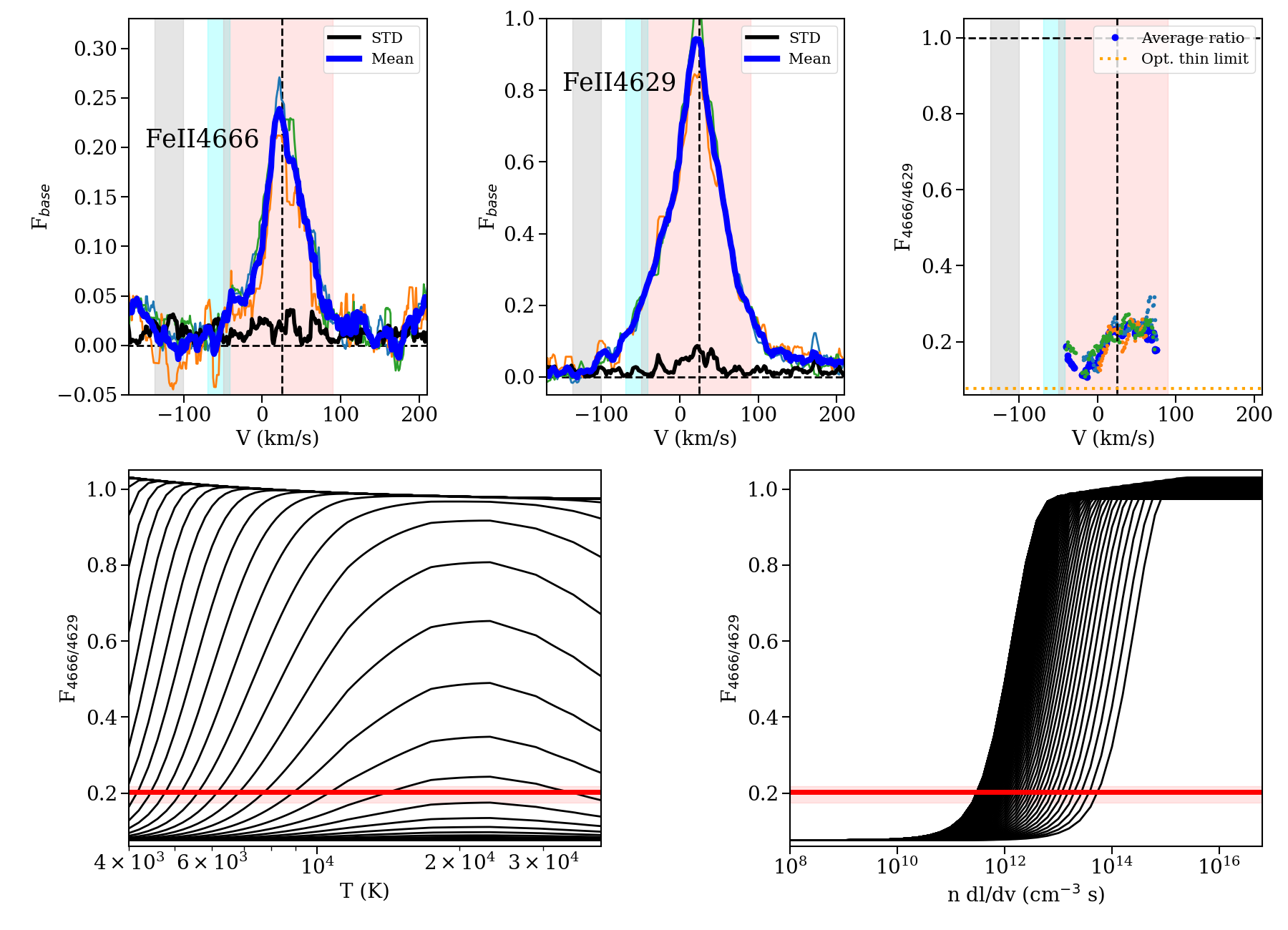
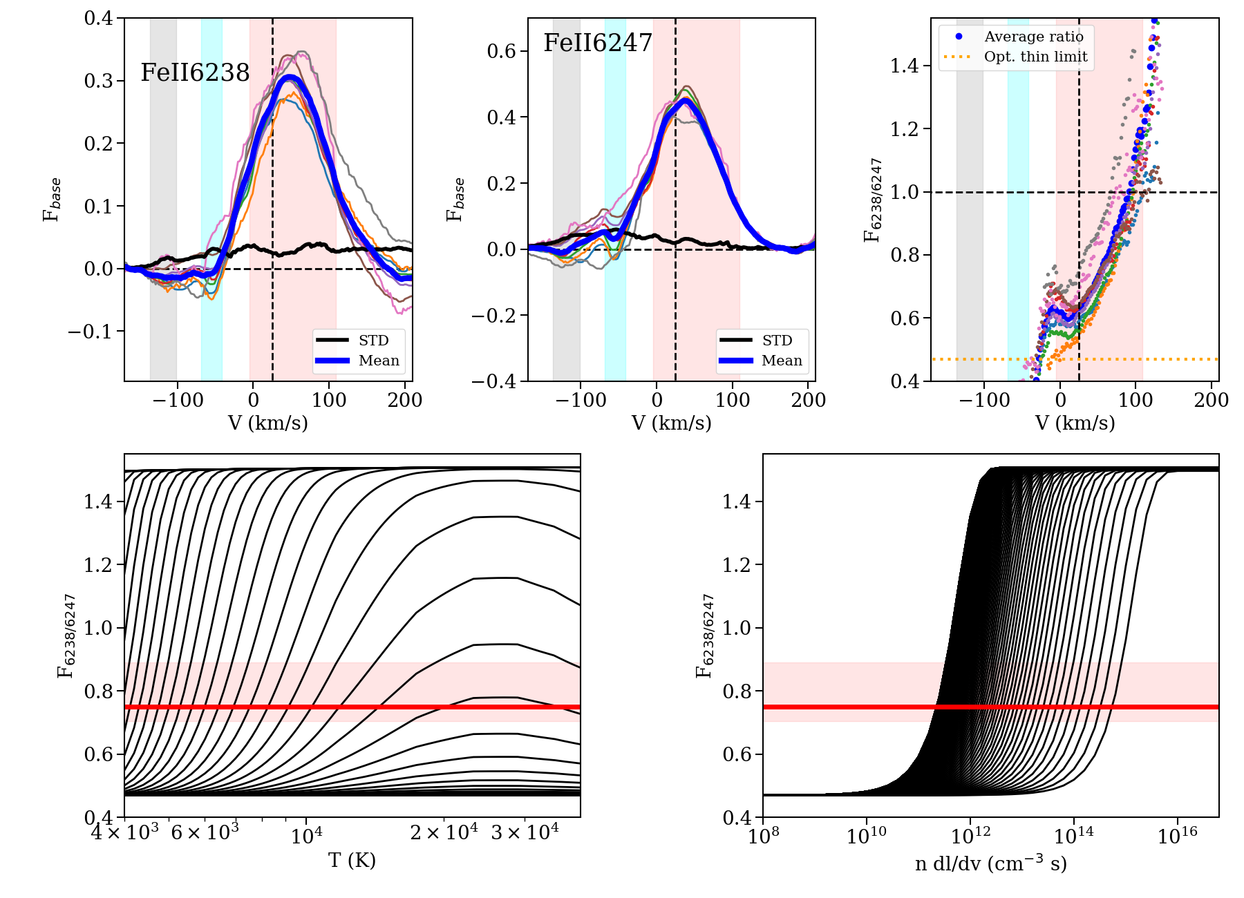
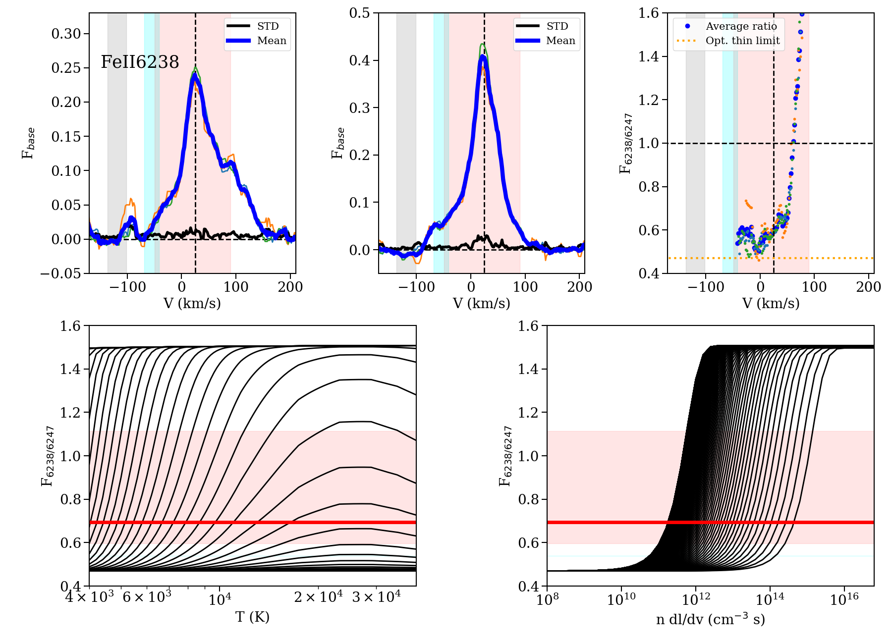
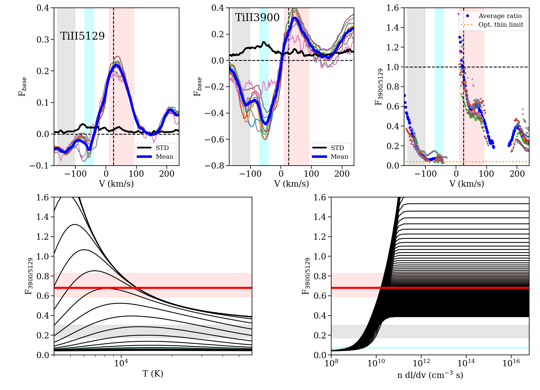
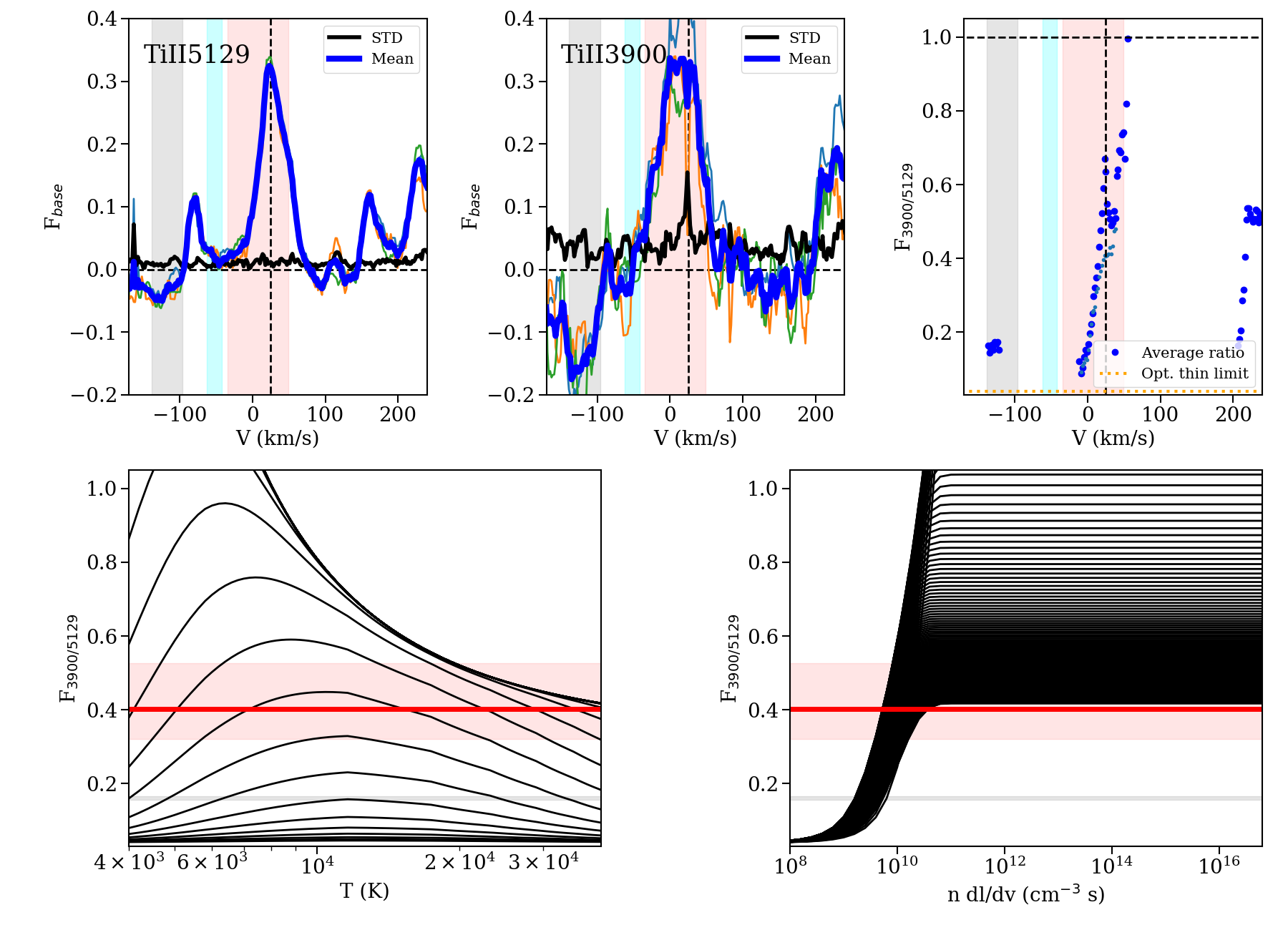
Figure 19: Analysis of the line ratio for the FeII and TiII lines with PCygni profiles from transitions with upper common levels (Figure 11, continued). The upper left panels show the line emission in outburst; the upper right panel shows the quiescence data. The ratios observed are compared to the theoretical calculations for a range of temperatures and column density-velocity gradients in the lower panels. In the velocity panels, the red area, cyan, and the gray area show the regions with significant redshifted emission, and slow and fast wind absorption, respectively. The shaded colored areas in the temperature and density planes show the regions that are compatible with the line ratios observed in the emission and the two wind component parts with their 1$\sigma$ error.

C.2 Disk analysis by brightness decomposition

To explore the location of the material producing the double-peaked emission lines, we used a procedure similar to Acke & van den Ancker (2006) to convert line intensity in each velocity bin into a relative brightness per unit area at each velocity. Assuming Keplerian rotation, we can convert the velocities into radial distances. One main limitation comes from gaseous disks being partly supported by their own gas pressure, so the rotation of hot atomic gas is sub-Keplerian. The thermal deviation from Keplerian rotation depends on the temperature, and this quantity ranges from $\sim$11 km s^-1 for a temperature of 10⁴ K, to $\sim$3.5 km s^-1 for a temperature of 10³ K. This is a small fraction of the total velocity span observed in the lines, justifying the approximation. We fit the ESPaDOnS data only, since the OHP data are too noisy for the fit.

For the brightness decomposition, we assume a disk inclination of 30 degrees and the outburst stellar values (R_∗=1.93 R_⊙, M_∗=16 M_⊙, L_∗=8$\times$2400 L_⊙). A different inclination or the stellar mass can be easily rescaled in the brightness decomposition plots, as long as the luminosity is kept constant. With these values we can estimate an effective temperature T_eff , assuming that the stellar radius does not change during outburst with respect to the quiescent value, that reproduces the observed luminosity. We can also estimate the temperature at various distances from the star, which depends on the heating mechanism and disk structure. We assume that the temperature of the innermost disk rim (the part producing the highest observed velocities) is set by direct irradiation, and for the rest of the disk it follows a power law with radius. Although the temperature estimate would be smaller if the emitting zone is larger (e.g., if the innermost disk is the emitting region), at larger distances the only quantity that matters is the total luminosity (or R${}_{emit}^{2}$T${}_{emit}^{4}$) as long as the emitting region is located at a smaller radius than the detected disk emission.

Fe I 6400 Å

Fe I 6462 Å

$\alpha$=-3/4	$\alpha$=-3/7	$\alpha$=-3/4	$\alpha$=-3/7

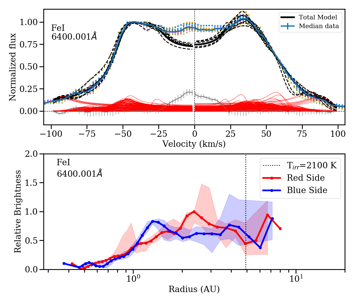
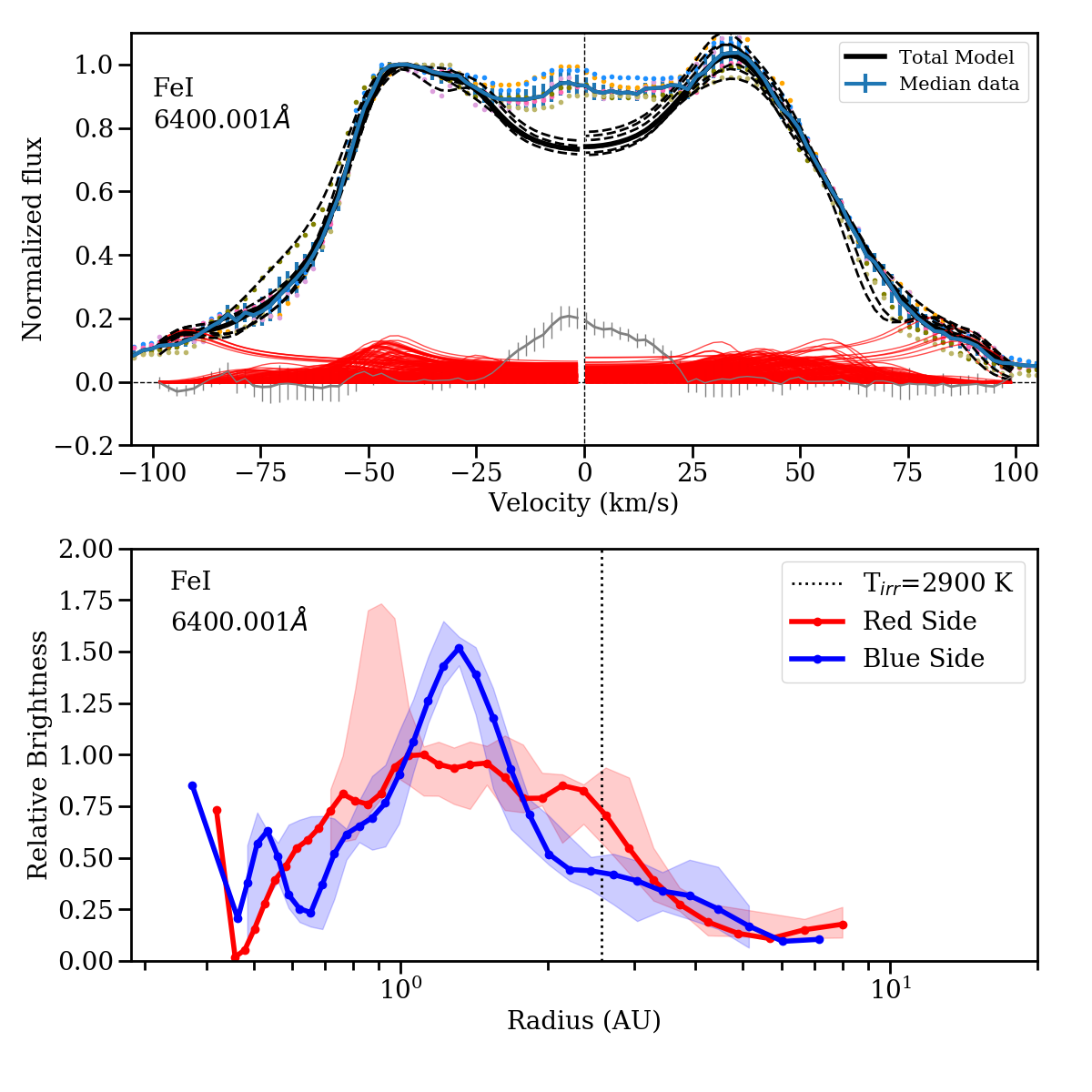
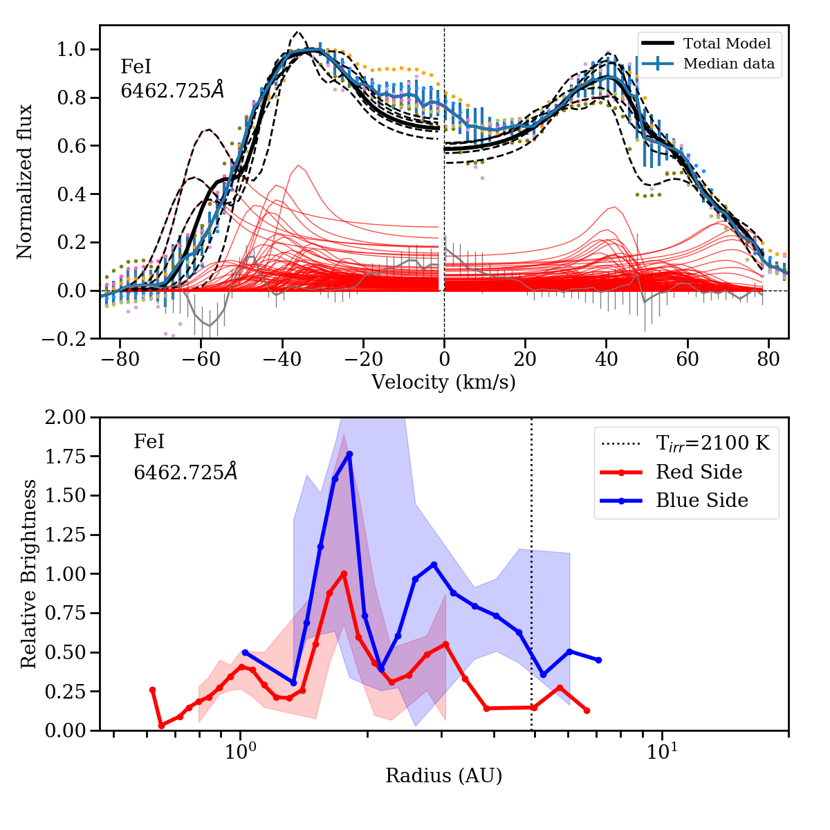
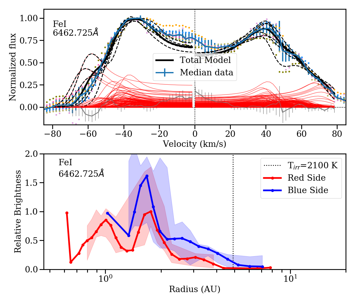
Figure 20: Examples of how the temperature power law affects the radius derived from the brightness profile. For each line, the left models show the results from a flat disk (power-law exponent -3/4; Chiang & Goldreich, 1997), while the right models show the results assuming a flared disk (power-law exponent -3/7; D’Alessio et al., 1999). The difference is larger for lines with higher transition probabilities (A_ki=9.3e6 s^-1 for FeI 6400Å, A_ki=5.6e4 s^-1 for FeI 6462Å) that are likely to be formed higher over the disk midplane. Colors and symbols as in Figure 13.

The temperature power law is poorly known, since we can have various sources of heating (e.g., irradiation, viscous dissipation) and gaseous disks are flared and have a vertical temperature structure. We tested several temperature versus radius power laws. These include the Chiang & Goldreich (1997) structure for an irradiated flat disk, for which the temperature in the disk is taken to be a power law of radius with exponent -3/4, which is also the same power law than if we assume a self-luminous disk powered by viscous dissipation (e.g., Hartmann, 1998); and the flared irradiated disk model, in which the temperature varies as a power law with an exponent -3/7 versus radius (D’Alessio et al., 1999). The result of using a steeper versus a shallower power law is that the strongest relative brightness moves to larger radii when the temperature decreases faster (i.e., if the temperature is lower, a larger area is needed to reproduce the observed flux), preserving the general shape of the profile and the blue/red (a)symmetry. Figure 20 shows some examples of the effect in the derived brightness profiles depending on the power law assumed. In general, the residuals of the flared disk models are smaller than those of the flat disk fits, thus we conclude that an irradiated flared disk model can fit better the velocity profiles observed, and this is what we use through Section 3.5.

Finding Fe I emission in LTE is unlikely at temperatures below a thousand degrees. For a flat, irradiated disk and the stellar luminosity in outburst, T=1000 K is reached at about 20 au. Even though other sources of heating (e.g., thermal dissipation due to accretion) are likely to operate in this strongly accreting system, we impose a cutoff at 35 au. Beyond this cutoff we deem that the emission becomes unreliable, especially for the strongest lines that often have an emission core at low velocities that cannot be separated from the disk emission. We also estimated the radial velocity of the line using the 80% level of the double peak of the line to estimate the line center, which typically produces radial velocity values between 20-35 km s^-1, in agreement with the narrow quiescence lines. A highly asymmetric line and/or eccentric or asymmetric disk could lead to inaccurate values of the radial velocity.

Following Acke & van den Ancker (2006), we decomposed the normalized line profile starting from the highest velocity at which the flux is $\geq$3$\sigma$. We assume that the emission at each velocity originates in a narrow ring located at the position with the same Keplerian orbital velocity. We generated simple disk model emission, assuming that each element of the velocity ring emits a line where the width is due to thermal broadening. The emission of the ring is proportional to the blackbody emission at the relevant temperature and to the area of the emitting ring. We constructed the emission of the ring by summing over all angles, breaking the ring into a 70 point grid in radius and azimuthal angle. The ratio of the observed to theoretical flux at each velocity point gives us the brightness associated with that ring. The resulting ring is subtracted from the total observed line, and the procedure is repeated for the next highest velocity until the line has been completely fitted or until we reach the 35 au cutoff.

The comparison between the blue and the red sides can provide information on the axisymmetry of the disk. In addition, this simple model allows to check whether there is emission at locations more distant than those expected to have a temperature of up to 2100 K (similar to the lower limit we obtained from Saha’s equation) for a directly irradiated disk. This would suggest that the disk is not (or not only) directly irradiated, but also heated by other mechanisms such as accretion, but in general the emission is very low at larger radii. The analysis is only valid if the line is not contaminated by nearby features and the continuum is relatively smooth. This results in only a subset of the lines with disk-like profiles being appropriate for the brightness decomposition, which is discussed in Section 3.5. A few examples of the brightness decomposition are shown in the main text; the rest of the lines can be found in Figure 21.

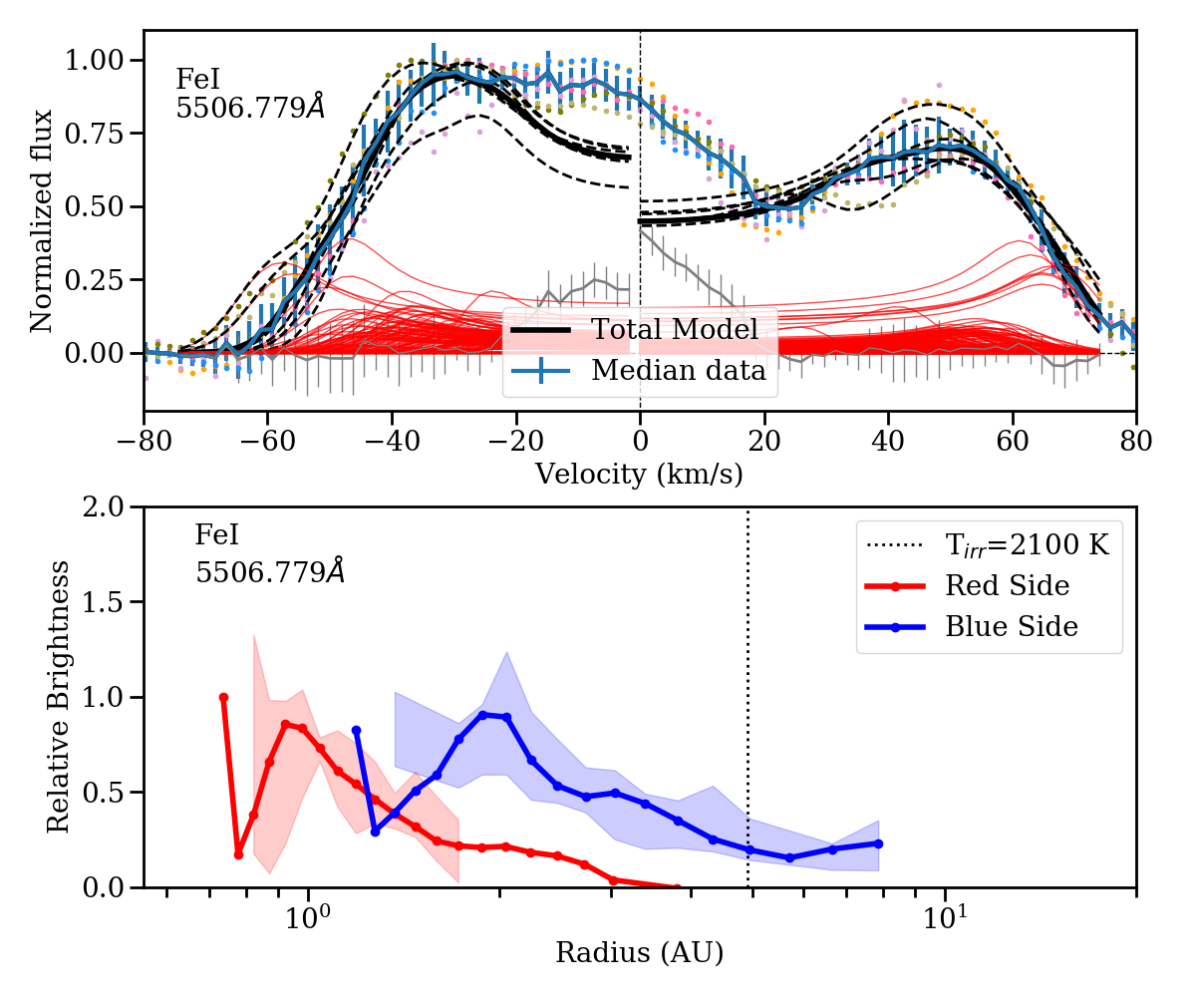
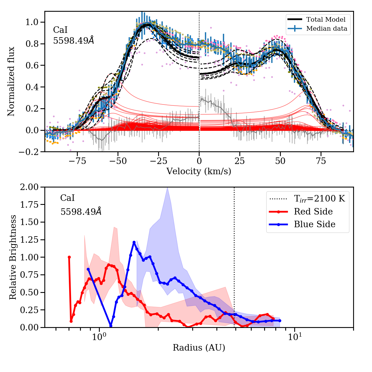
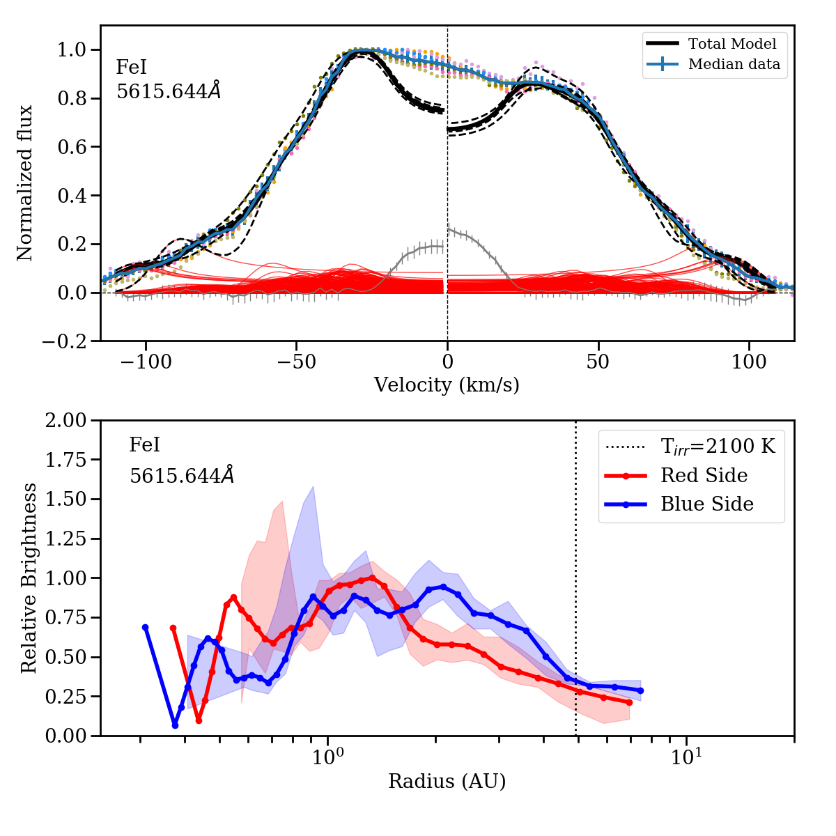
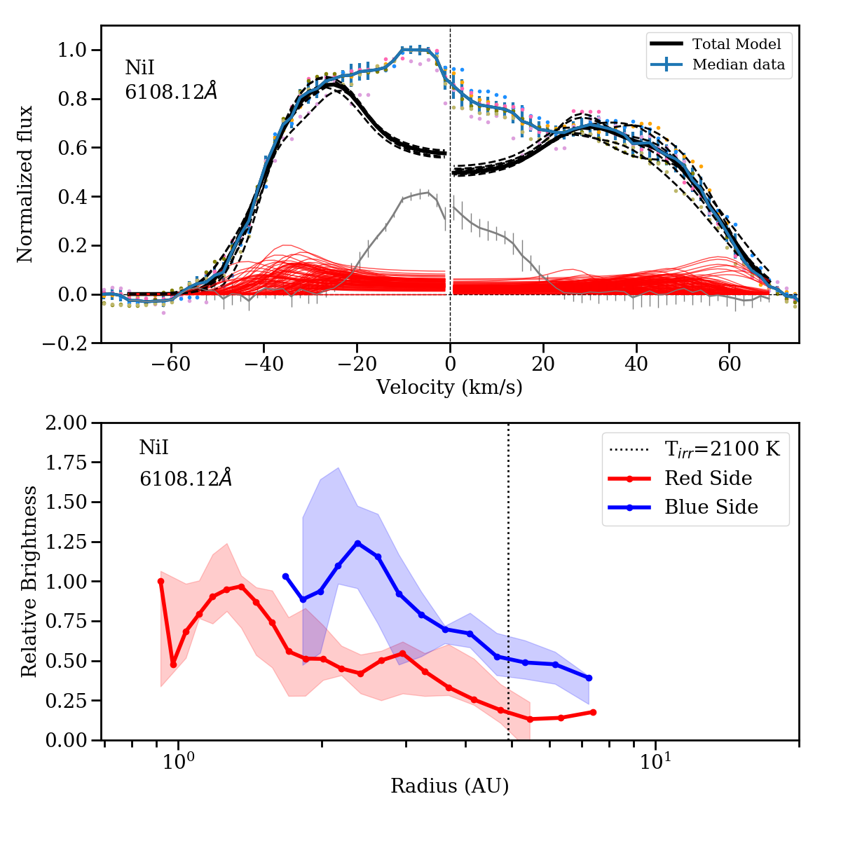
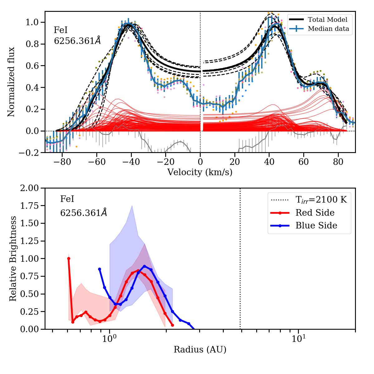
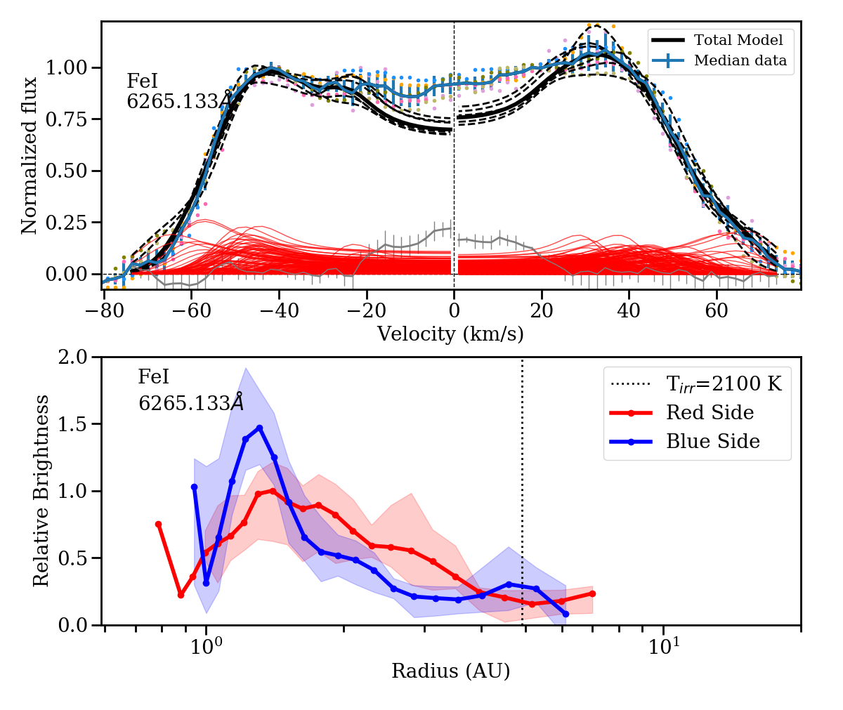
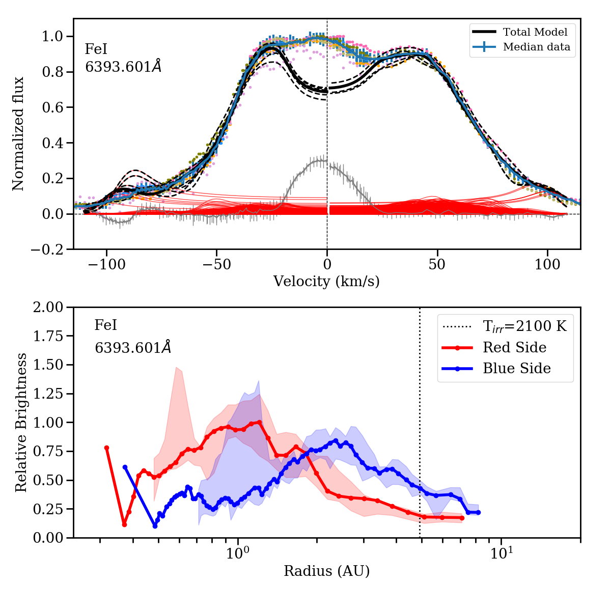
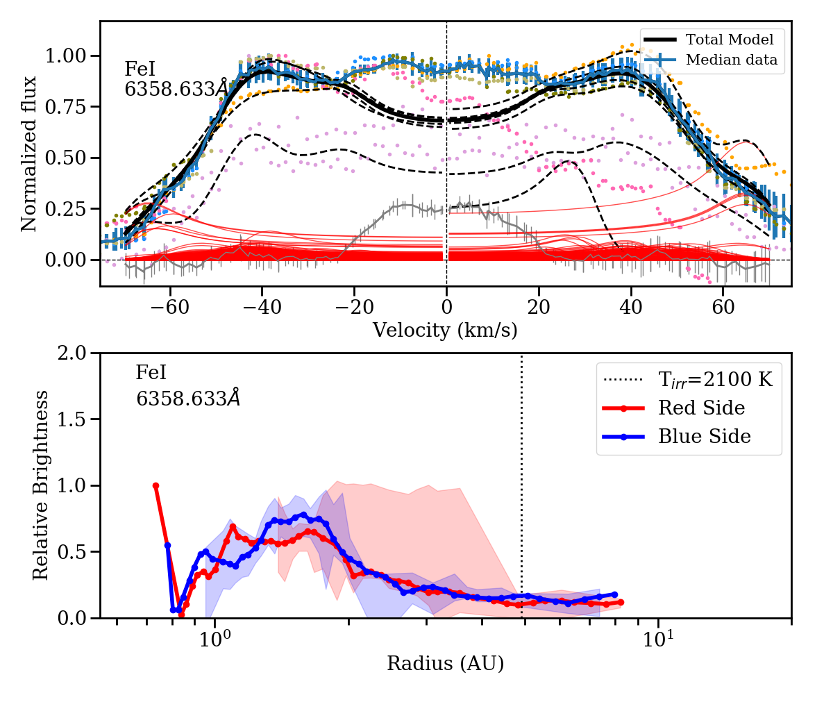
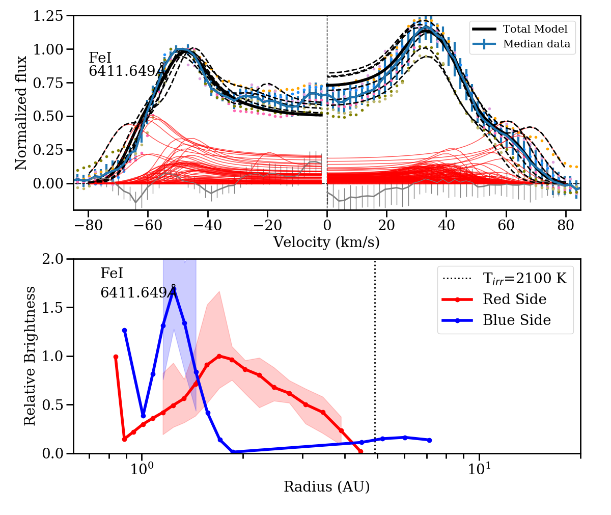
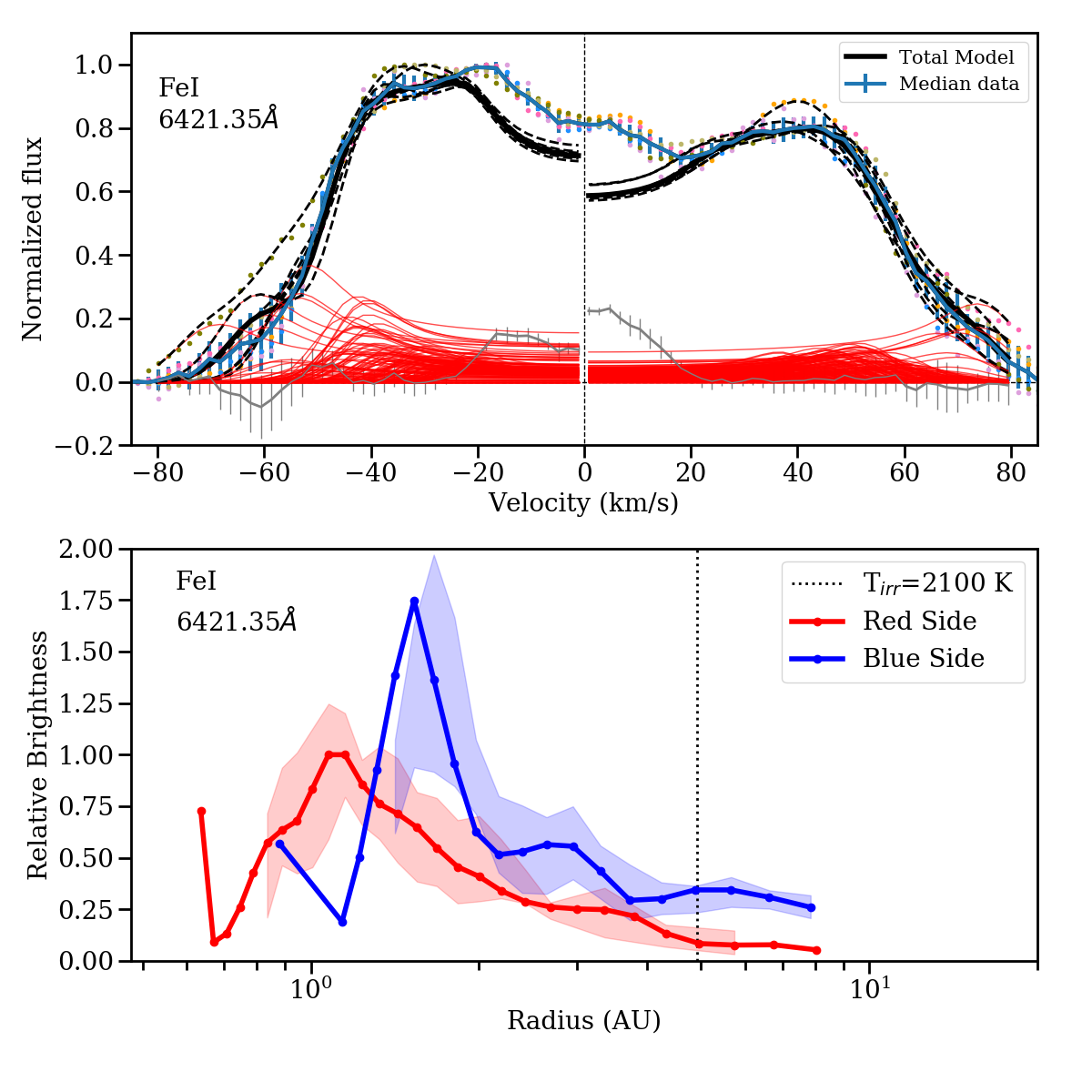
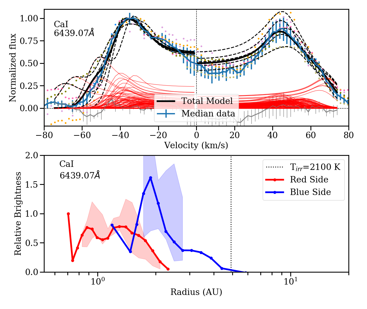
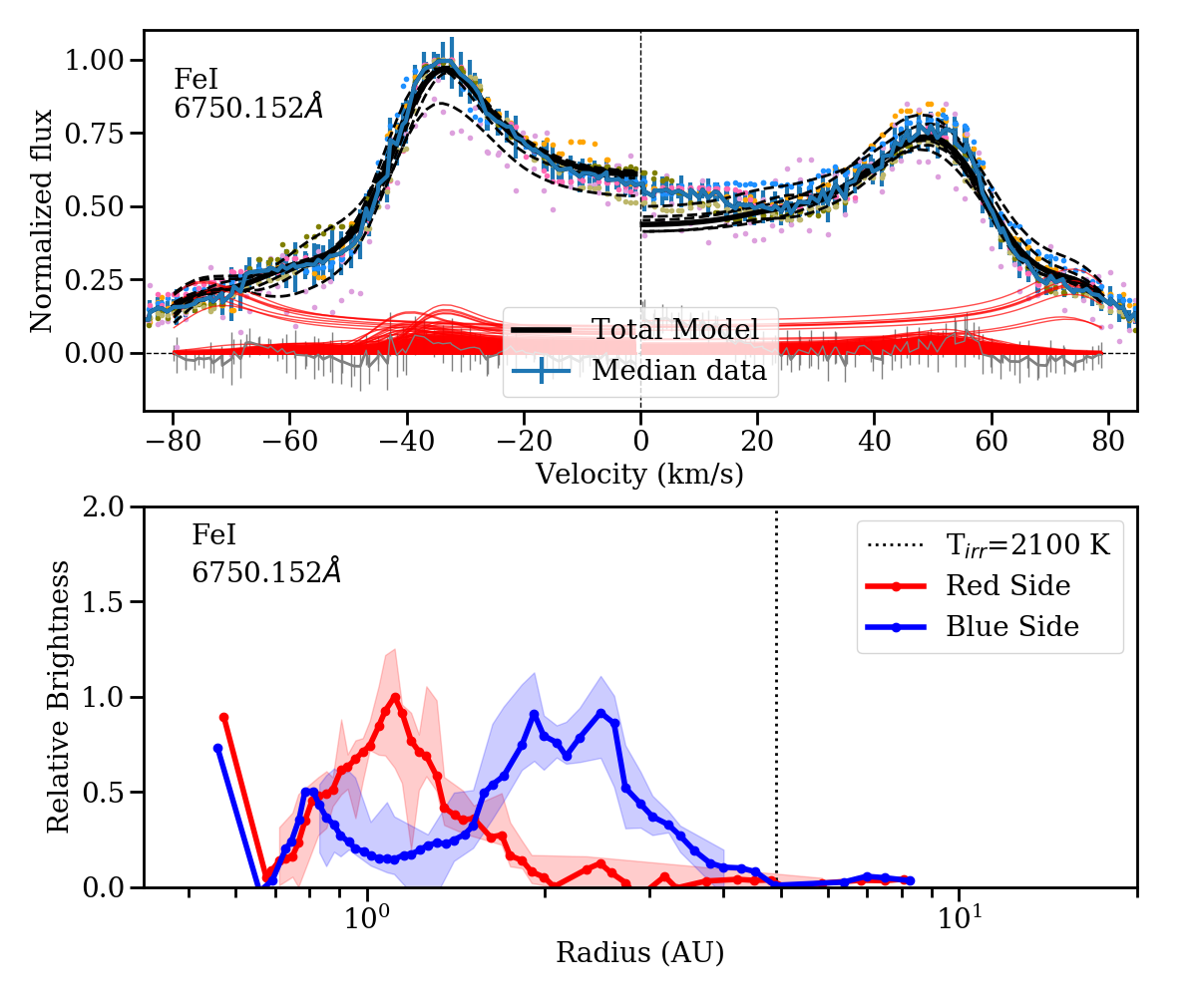
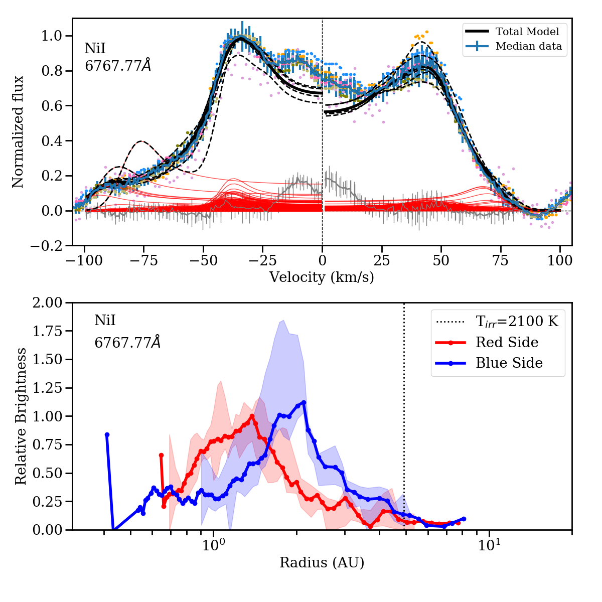
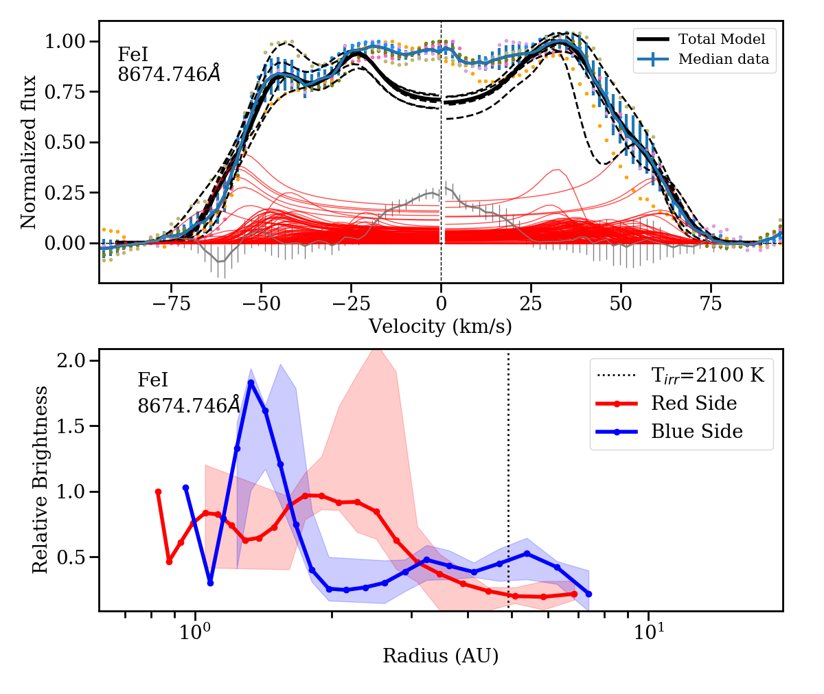
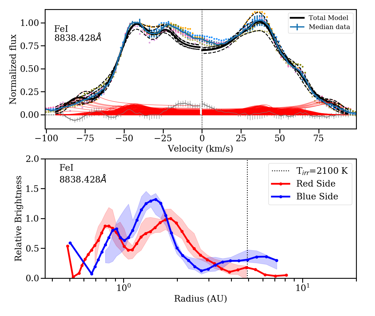
Figure 21: Brightness profile decomposition for the disk-like lines not shown in the main text (Figure 13, continued). For each line, the upper panel shows the normalized, median line emission (blue), individual data points (colored dots), and model fit. The black solid line represents the best fit to the median data, while the dashed lines indicate the fits to the individual datasets that are used to compute the errors. The zero velocity (measured with respect to the symmetry axis of the line) is shown as a dotted line. The individual ring fits are shown by thin red lines, and the residuals are shown in gray. Since we impose a limit of 35 au to avoid fitting potential narrow emission within the line, the center of the line is not well fitted. In the lower panel for each line, the red and blue thick lines show the best fit to the median spectrum for the red and blue sides, while the shaded areas show the range spanned by the fits to the individual spectra. Because the noise in the single spectra is higher than in the median spectrum, there are no significant results at extreme velocities for some of the individual datasets. The vertical dotted line indicates the place where direct irradiation results in a temperature of 2100 K, which is independent of the model assumptions and stellar mass. All models are calculated for an inclination of 30 degrees and a stellar mass of 16 M_⊙. A different inclination $i$ would change the derived radii by sin${}^{2}i$/sin${}^{2}(30)$, and a different stellar mass M_∗ would change the derived radii by a factor of M_∗/16M_⊙, but the relative brightnesses would remain the same.

Table B.1: Emission lines observed during outburst and quiescence. The lines are classified as “double-peaked” or disk-like (Dsk), “PCygni profiles” (PC). Those with complex, multicomponent wind absorption signatures are denoted as ’PC+’. Potential blends and contamination by atmospheric features are denoted by ”Bl” and ”Atm”, respectively. Those that could not be classified are labeled as ”INDEF”, and in some cases, a potential identification is given in the notes. The wavelengths provided are laboratory measurements (air), except for non-identified lines, for which we list the observed wavelengths. If the line is not seen, it is denoted as ’N’, except if this part of the spectrum was not covered or if other features may have difficulted the identification, in which case we denote it as ’-’. Lines denoted with vdA04 have been observed by van den Ancker et al. (2004) during the 1999 outburst. Lines denoted with WS have been identified using Wahlgren & Shore (S. Shore, private communication), while the rest have been identified with the NIST database. Lines that are potentially pumped by other UV lines (Herczeg et al., 2005) are listed accordingly. For some of the close blends without clear peaks, the species cannot be easily identified. We note that the quiescence data had a lower spectral coverage, ending at $\sim$6940Å.

Species	$\lambda_{air}$	Aki	Ei	Ek	Outb.	Quies.	Type	Notes
	(Å)	(s-1)	(eV)	(eV)
FeI	3701.086	6.35E+07	2.998	6.347	Y	-
FeI	3704.461	1.42E+07	2.692	6.038	Y	-
TiII:	3706.230	3.10E+07	1.566	4.910	Y	-		WS. No TiII at 3819, 3833.5Å.
FeI	3709.246	1.56E+07	0.915	4.256	Y	-
MnI	3708.856	5.20E+06	4.666	8.008	Y	-		May be pumped by CIV
HI	3711.978	9.21e+03	10.199	13.538	Y	-	Wk
INDEF	3715.7	—	—	—	Y	-		VI 3714.9Å?
CaII:	3736.900	1.70E+08	3.151	6.468	Y	-	Wk
INDEF	3742.5	—	—	—	Y	-		VI 3741.5Å?
HI	3750.151	2.83e+04	10.199	13.504	Y	-	PC,Bl
FeI	3761.408	1.04E+06	2.588	5.883	Y	-
TiII	3761.320	9.90E+07	0.574	3.869	Y	-
HI	3770.633	4.40e+04	10.199	13.486	Y	-	PC
FeI/TiII	3774-6	—	—	—	Y	-	Bl
NiI	3783.530	3.30E+06	0.423	3.699	Y	-
FeI/NiI	3787	—	—	—	Y	-	Bl
HI	3797.909	7.1225e+04	10.199	13.462	Y	-	PC
NiI	3807.140	4.30E+06	0.423	3.678	Y	-	Bl
FeI	3815.840	1.12E+08	1.485	4.733	Y	-
FeI	3821.178	5.54E+07	3.267	6.511	Y	-
HI	3835.395	1.22e+05	10.199	13.431	Y	-	PC
FeI	3841.048	1.36E+08	1.608	4.835	Y	-
FeI	3849.966	6.05E+07	1.011	4.231	Y	-
FeI	3859.911	9.69E+06	0.000	3.211	Y	-
CaI/FeI	3873	—	—	—	Y	-	Bl
FeI	3879	—	—	—	Y	-	Bl
HI	3889.064	2.2148e+05	10.199	13.386	Y	N	PC
TiII	3900.540	1.60E+07	1.131	4.308	Y	Y	PC+	EXL-q
INDEF	3903	—	—	—	Y	Y	Wk
FeII	3905.626	4.00E-03	0.048	3.221	Y	Y
FeI/CrI	3913-6	—	—	—	Y	Y	Bl, Wk	PC, could be FeII
FeI	3922.912	1.08E+06	0.052	3.211	Y	N		EXL-q
CaII	3933.660	1.47E+08	0.000	3.151	Y	Y	PC+	vdA04
FeII	3938.290	6.10E+03	1.671	4.818	Y	Y	PC
FeI/CoI	3944-5	—	—	—	Y	Y	Bl
CoI	3952.318	2.20E+05	0.432	3.568	Y	Y
CaI/Fe	3957.0	—	—	—	Y	Y	Bl
CaII	3968.470	1.40E+08	0.000	3.123	Y	N	PC	Blend with HI
FeII	3974.167	6.30E+03	2.704	5.823	Y	N
FeI	3977.741	6.41E+06	2.198	5.314	Y	Y		EXL-q
MnI	3982.157	3.50E+07	4.273	7.386	Y	Y	Bl
MnI/CrI/CoI	3987-91	—	—	—	Y	N	Bl
FeI/CoI	3997.4-.9	—	—	—	Y	Y	Bl	EXL-q
FeI	4001.662	7.47E+05	2.176	5.273	N	Y	Wk
MnI	4003.260	1.10E+07	4.640	7.736	Y	N		Pumped by UV FeII?
FeI:	4005.242	2.04E+07	1.557	4.652	Y	Y		EXL-q
INDEF	4013.0				Y	N	PC	WS. TiII 4012.39Å? VI 4012.495Å?
FeI	4013.782	4.19E+05	3.017	6.105	Y	Y
INDEF:	4023.7	—	—	—	N	Y	Wk	WS. HeI 4023.98Å?
TiII	4025.140	5.40E+05	0.607	3.687	Y	Y
TiII	4028.343	5.14E+06	1.89	4.97	Y	N	PC	WS
FeI/MnI	4030.8-9	—	—	—	Y	Y	Bl	Several lines
FeI	4033.186	8.40E+04	2.559	5.632	Y	N
TiII	4028.343	5.1e+06	1.892	4.969	Y	Y	PC
NiI	4035.949	4.80E+05	3.655	6.726	Y	N
FeI	4045.812	8.62E+07	1.485	4.549	Y	Y		13db, EXL-q
TiII	4053.834	4.20E+06	1.893	4.950	Y	Y	PC
FeI	4062-3	—	—	—	Y	Y	Bl	13db, EXL-q
FeI	4067.271	2.19E+06	2.559	5.607	Y	Y	Bl, Wk
FeI/TiII	4071-2	—	—	—	Y	Y	PC,Bl
CrI	4077.680	—	—	—	Y	Y		13db, EXL-q
FeI	4083.549	1.84E+05	2.279	5.314	Y	N
SiI	4102.936	6.09E+04	1.909	4.930	Y	Y
H$\delta$	4101.710	9.73e+05	10.199	13.220	Y	Y	PC+
CoI	4110.540	5.50E+06	1.049	4.064	Y	Y
MnI	4113.867	1.50E+07	4.354	7.367	Y	N	Bl
MnI	4114.384	1.50E+07	4.345	7.357	Y	N	Bl
FeI	4118.886	1.90E+06	3.266	6.275	Y	Y
FeI	4123.728	6.04E+05	2.990	5.996	Y	Y
FeII	4128.748	2.60E+04	2.583	5.585	Y	Y	PC
FeI	4132.058	1.18E+07	1.608	4.608	Y	Y		13db, EXL-q
FeI	4134.677	1.25E+07	2.832	5.829	Y	Y		EXL-q
FeI	4143.868	1.33E+07	1.557	4.549	Y	Y		EXL-q
FeI:	4150.249	7.70E+06	3.430	6.417	Y	Y	Bl	WS. Blend with FeII 4150Å.
FeI	4154.805	1.40E+07	3.368	6.352	Y	Y
FeI	4156.798	1.20E+07	2.832	5.813	Y	Y
FeI	4161.077	9.50E+05	3.368	6.347	Y	Y
TiII	4163.348	2.55E+07	2.590	5.567	Y	N	PC	WS
FeI	4172.122	9.80E+06	3.251	6.222	N	Y	Bl
FeII	4173.461	4.43E+05	2.583	5.553	Y	Y		EXL-q
FeI	4175.636	1.14E+07	2.845	5.813	N	Y	Wk
FeI	4177.594	3.71E+04	0.915	3.882	N	Y	Bl	EXL-q
FeII	4178.862	1.72E+05	2.583	5.549	Y	Y	PC	EXL-q
FeI	4181.754	2.32E+07	2.832	5.796	Y	Y
FeI	4184.891	1.03E+07	2.832	5.793	Y	N
FeI	4187.6-.8	—	—	—	Y	N	Bl
FeI	4191.4-.7	—	—	—	Y	Y	Bl,Wk	13db, EXL-o, EXL-q
FeI	4195.618	1.21E+06	3.017	5.972	Y	Y
FeI	4199.095	4.92E+07	3.047	5.999	Y	Y
FeI	4202.029	8.22E+06	1.485	4.435	Y	Y		EXL-o, EXL-q
FeI	4203-4	—	—	—	N	Y	Wk, Bl
FeI	4205.538	2.77E+06	3.417	6.364	Y	Y
INDEF	4209.646	-100	—	—	Y	N	Wk	WS. Nearby [FeII] at 4208.82Å
FeI	4216.184	1.84E+04	0.000	2.940	Y	Y		EXL-q
FeII	4233.167	7.22E+05	2.583	5.511	Y	Y	PC+	13db, EXL-o, EXL-q, vdA04
CrI/FeI/FeII	4238.8-.9	—	—	—	Y	N	Bl	EXL-q
CrII	4246.409	3.73e+04	3.854	6.773	Y	Y	PC+	Redshifted
FeI	4250.787	1.02E+07	1.557	4.473	Y	N		EXL-q
FeI	4254.945	1.43E+05	3.018	5.931	Y	Y
FeII	4258.154	3.10E+04	2.704	5.615	Y	Y		EXL-q. Low Aki, weak PC.
CrI	4262.373	2.40E+06	3.079	5.987	Y	Y	Wk
FeII	4273.326	9.10E+04	2.704	5.605	Y	Y	PC,Bl	13db, EXL-q
FeI	4275.698	5.59E+04	2.559	5.458	Y	N
FeI	4278.231	1.00E+06	3.368	6.265	Y	Y		vdA04
FeI	4282.403	1.21E+07	2.176	5.070	Y	Y		EXL-q
TiI:	4287.400	1.46E+07	0.836	3.727	N	Y	Wk, Bl
TiII	4290.230	4.6E+06	1.165	4.054	Y	Y	PC	vdA04
TiII:	4294.099	4.68E+06	1.084	3.971	Y	Y	PC,Bl	EXL-q,WS, vdA04. Blend with FeI/FeII
FeII	4296.572	7.00E+04	2.704	5.589	Y	Y	PC	EXL-q
TiII	4300.050	7.70E+06	1.180	4.063	Y	Y	PC+	EXL-q
TiII	4301.930	6.20E+06	1.161	4.042	Y	Y		EXL-q
FeI	4302.185	7.70E+05	3.047	5.928	N	Y
FeII	4303.176	2.20E+05	2.704	5.585	Y	Y	PC	EXL-q
TiII	4307.900	4.60E+06	1.165	4.042	Y	Y	PC	EXL-q, vdA04
TiII	4312.870	4.10E+06	1.180	4.054	N:	Y	Bl	EXL-q
TiII	4314.975	1.30E+07	1.161	4.033	Y	Y	PC,Bl
TiII	4320.960	2.40E+06	1.165	4.033	Y	Y	PC	vdA04
FeI/CrI	4325	—	—	—	Y	Y	Bl	13db, EXL-q
H$\gamma$	4340.472	2.53e+06	10.199	13.054	Y	Y	PC	13db, EXL-q, EXL-o, vdA04
TiII	4344.290	7.20E+05	1.084	3.937	Y	N	Wk
FeII	4351.769	4.66E+05	2.704	5.553	Y	Y	PC	WS, vdA04. Near FeI and [FeII]
[FeII]/FeII	4358-62	—	—	—	N	Y	Wk,Bl	WS, vdA04
TiII/FeI/FeII	4367-9	—	—	—	Y	Y	Bl	EXL-q, vdA04
FeI	4375.930	2.95E+04	0.000	2.833	N	Y		13db, EXL-q. Blend with TiII
TiII	4374.815	3.00E+06	2.061	4.894	Y	Y	Bl	vdA04. Blend with FeII
FeI	4383.545	5.00E+07	1.485	4.312	N	Y		13db, EXL-q
FeII	4385.387	4.50E+05	2.778	5.605	Y	Y	Bl	EXL-q, vdA04
TiII	4386.844	2.40E+06	2.598	5.423	N	Y	Bl
TiII	4395.850	2.90E+05	1.243	4.063	Y	Y	Bl,PC	Blend with FeII and TiII 4395Å
ScII	4400.389	1.52E+07	6.908	9.730	Y	N	PC+	WS. Pumped by UV H2?
FeI	4404.750	2.75E+07	1.557	4.371	Y	Y	Bl	EXL-q
FeI/MnI/TiII	4407-9	—	—	—	Y	Y	Bl	Some lines unblended in quiescence
FeI/TiI/FeII	4415-17	—	—	—	N	Y	Bl	13db, EXL-q, vdA04
TiII	4418.330	3.00E+05	1.237	4.042	Y	Y	Bl
FeI	4422.568	8.72E+06	2.845	5.648	Y	Y
FeI	4427.310	3.41E+04	0.052	2.851	Y	Y
FeI	4430.614	7.45E+06	2.223	5.020	Y	Y	Bl	EXL-o,
NiI	4431.033	4.10E+06	4.167	6.965	Y	Y	Bl
TiII	4443.800	1.1E+07	1.080	3.869	Y	Y	PC,Bl	Blend of TiII
TiII	4444.558	3.90E+05	1.116	3.904	Y	Y	PC,Bl	Blend of TiII
FeI	4447.130	8.91E+04	2.198	4.985	Y	Y	Bl	Unblended in quiescence
FeI	4447.717	5.11E+06	2.223	5.010	Y	Y	Bl	Unblended in quiescence
TiII	4450.490	2.00E+06	1.084	3.869	Y	Y	PC+	EXL-q. Shallower than TiII 4443Å
FeI	4455.027	4.10E+06	3.882	6.664	Y	Y	Bl
FeI	4459.117	2.52E+06	2.176	4.956	Y	Y		EXL-q
FeI	4461.970	2.31E+06	3.603	6.380	Y	Y
TiII	4464.450	7.00E+05	1.161	3.937	N	Y	Wk
TiII	4468.500	1.00E+07	1.131	3.904	Y	Y	PC+	13db, EXL-q, vdA04
INDEF	4473.8	—	—	—	Y	N		VI 4473Å:
FeI	4476.018	1.01E+07	2.845	5.614	N	Y
FeI/CrI	4482	—	—	—	Y	Y	Bl	13db:, Several lines
FeII	4489.183	5.90E+04	2.828	5.589	Y	Y	Bl	13db, EXL-q, vdA04. Low Aki, no PC
FeII	4491.405	1.89E+05	2.856	5.615	Y	Y	Bl	EXL-q, vdA04
FeI	4494.563	3.45E+06	2.198	4.956	Y	Y	Bl	EXL-q
TiII	4501.270	9.80E+06	1.116	3.869	Y	Y	PC	EXL-q, vdA04
FeII	4508.288	7.30E+05	2.856	5.605	Y	Y	PC	EXL-q
FeII	4515-6	—	—	—	Y	N	PC	FeII blend, WS, vdA04
FeI	4518.432	2.10E+04	3.237	5.980	N	Y	Wk
FeII	4520.224	9.80E+04	2.807	5.549	Y	Y	PC	EXL-q, vdA04
FeII	4522.634	8.40E+05	2.844	5.585	Y	Y	PC	vdA04
TiII	4529.474	3.00E+05	1.572	4.308	Y	Y		13db. Weaker than other TiII
TiII/FeII	4534	—	—	—	Y	Y	Bl	vdA04
FeII	4549.474	1.00E+06	2.828	5.553	Y	Y	Bl, PC+	13db, EXL-o, EXL-q, vdA04
TiI	4552.460	2.10E+07	0.836	3.559	N	Y
CrI/FeI/FeII	4556				Y	Y	Bl
CrII	4558.660	8.80E+06	4.073	6.792	Y	Y	PC+	EXL-q, vdA04. Similar to TiII
TiII	4563.770	8.80E+06	1.221	3.937	Y	Y	BC	EXL-o, EXL-q
TiII	4571.980	1.20E+07	1.572	4.283	Y	Y	PC+	vdA04
FeII	4576.340	6.40E+04	2.844	5.553	Y	Y		EXL-q, vdA04
CoI	4580.131	2.70E+04	0.923	3.629	N	Y	Wk
FeII	4583.829	7.22E+05	2.807	5.511	Y	Y	Bl	vdA04
CrII	4588.199	1.20E+07	4.071	6.773	N	Y	PC	vdA04
TiII	4589.950	1.30E+06	1.237	3.937	Y	Y	Bl	EXL-q
FeI/CrI/FeII	4592	—	—	—	Y	N	Bl
FeI	4592.651	1.61E+05	1.557	4.256	N	Y	Bl	EXL-q. Only in quiescence
FeI	4603	—	—	—	Y	Y	Bl	Multiple blend
CrII	4616.629	4.00E+06	4.072	6.757	N	Y	Wk,Bl
FeII/FeI/CrII	4617-20	—	—	—	Y	Y	Bl
FeII	4629.339	1.72E+05	2.807	5.484	Y	Y	PC	13db, EXL-o, EXL-q, vdA04
CrII	4634.070	8.90E+06	4.072	6.747	Y	Y	PC	vdA04. Weak PC, near FeII
CrI	4639.520	9.50E+06	3.111	5.782	N	Y	Wk
FeI	4654.498	5.64E+04	1.557	4.220	N	Y
CrI	4656.809	1.10E+07	4.778	7.440	Y	Y	Bl	May be pumped by [OIII]
TiII	4657.206	2.70E+05	1.243	3.904	Y	Y
[FeII]	4664.440	1.47E-01	0.121	2.778	Y	N		WS Blueshifted
FeII	4666.758	1.30E+04	2.828	5.484	Y	Y		13db, EXL-q. Low Aki, no PC.
FeII	4670.182	3.20E+03	2.583	5.237	Y	Y		Low Aki, no PC.
FeI	4691.411	1.01E+06	2.990	5.632	Y	Y	Dsk
CoI	4699.177	7.40E+03	1.049	3.687	Y	Y	Dsk
MgI:	4702.991	2.19E+07	4.346	6.981	Y	N	Dsk	EXL-o, EXL-q, offset
FeI	4708.968	3.98E+05	3.640	6.272	Y	Y	Dsk	vdA04
FeI	4710.283	1.05E+06	3.018	5.649	N	Y
[FeII]	4728.068	4.53E-01	0.083	2.704	Y	Y
FeII	4731.453	2.80E+04	2.891	5.511	Y	Y	PC	13db, EXL-q, vdA04
FeI	4733.591	3.41E+04	1.485	4.103	N	Y	Bl:	Only in quiescence
TiII	4762.776	7.20E+04	1.084	3.687	N	Y	Wk,PC
CrI	4764.626	7.30E+05	3.013	5.615	Y	Y
TiII	4779.985	6.20E+06	2.048	4.641	Y	Y	PC
FeI	4786.807	1.03E+06	3.017	5.607	Y	Y	Dsk
FeI	4789.650	4.57E+06	3.547	6.134	Y	N	Dsk
FeI	4791.246	3.56E+05	3.274	5.861	Y	Y	Dsk
FeI/TiII	4798	—	—	—	Y	Y	Bl
TiII	4805.100	1.10E+07	2.061	4.641	Y	Y	PC	EXL-o, vdA04
FeI/TiI/CrII	4811-4	—	—	—	Y	Y	Bl	vdA04
CrII	4824.127	1.70E+06	3.871	6.440	Y	Y	PC+	EXL-o, EXL-q, vdA04. Strong PC.
FeII	4833.197	4.60E+02	2.657	5.222	Y	Y		Low Aki, no PC FeII
FeI	4835.868	1.10E+06	4.103	6.667	Y	Y	Dsk
FeI	4839.544	3.90E+05	3.267	5.828	Y	N	Dsk
CrII	4848.235	2.60E+06	3.864	6.421	N	Y		EXL-o, EXL-q
H$\beta$	4861.350	8.42e+06	10.199	12.749	Y	Y		13db, EXL-o, EXL-q, vdA04
CrII	4876.473	1.60E+06	3.864	6.406	-	Y		EXL-q, vdA04. Blend with H$\beta$ in outburst.
FeI	4873.751	5.50E+04	3.301	5.844	-	Y		Blend with H$\beta$ in outburst
CrII	4884.607	5.80E+05	3.858	6.396	Y	Y
FeI	4891.492	3.08E+07	2.851	5.385	Y	Y
FeII	4893.820	2.50E+03	2.828	5.361	Y	N	Wk	Low Aki, no PC, very weak
NiI:s	4900.971	5.00E+05	3.480	6.009	Y	Y
FeI	4903.310	6.58E+06	2.882	5.410	Y	N	Dsk,Bl
TiII	4911.193	3.20E+07	3.124	5.647	Y	Y		EXL-o
FeII	4923.921	4.28E+06	2.891	5.408	Y	Y	PC+	13db, EXL-q, vdA04
INDEF	4934.505	—	—	—	Y	Y
FeI:	4939.686	1.39E+04	0.859	3.368	Y	Y	Dsk,Bl	13db
FeI	4957.596	4.22E+07	2.808	5.308	Y	Y	Dsk:	Dome-shaped
TiI	4981.730	6.60E+07	0.848	3.337	Y	Y	Bl
FeI	4985.253	1.48E+07	3.929	6.415	Y	N	Bl
FeII	4989-90	—	—	—	N	Y	Bl, Wk
FeII	4993.358	6.90E+03	2.807	5.289	Y	Y	Bl	13db, vdA04
NiI	5000.340	1.40E+07	3.635	6.114	Y	Y	Bl
FeI	5001.863	3.70E+07	3.882	6.360	Y	Y	Bl,Dsk	Maybe contaminated by TiI
FeII	5018.434	2.00E+06	2.891	5.361	Y	Y	PC+	13db, EXL-o, EXL-q, vdA04
INDEF	5031.9	—	—	—	Y	Y	Dsk	Likely FeI. Nearby ScII
TiI	5036.470	3.94E+07	1.443	3.904	Y	Y
TiI	5038.400	3.87E+07	1.430	3.890	Y:	Y		Very weak in outburst
FeI	5041.071	4.29E+04	0.958	3.417	Y	Y	Bl	13db. Blended in outburst, near CaI
FeI	5041.756	2.35E+05	1.485	3.943	Y	Y	Bl	13db. Blended in outburst
FeI	5049.819	1.65+06	2.279	4.733	Y	Y	Bl	Blended in outburst
FeI	5051.634	4.65E+04	0.915	3.368	Y	Y	Dsk,Bl	13db
FeI	5065.192	8.86E+05	3.642	6.089	Y	N	Dsk
FeI	5068.766	3.37E+06	2.940	5.385	Y	Y	Dsk
CrI	5072.920	1.59E+05	0.941	3.385	Y	Y	Dsk
FeI	5079.740	5.19E+04	0.990	3.430	Y	Y	Dsk	Maybe contaminated by other Fe I lines
FeI	5083.338	4.06E+04	0.958	3.397	Y	Y	Dsk	13db
FeI	5098.698	4.83E+05	2.176	4.607	Y	Y	Dsk, Bl
INDEF	5101.615	—	—	—	Y	Y
NiI	5102.966	8.80E+04	1.676	4.105	N	Y
FeI	5107	—	—	—	Y	Y	Bl	Two lines
FeI:	5107.447	4.18E+04	0.990	3.417	N	Y	Bl	Blend of several Fe I lines
FeI	5110.413	4.93E+03	0.000	2.425	Y	Y	Dsk	13db. Low-density line
FeII	5120.352	2.59e+03	2.828	5.249	Y	Y		WS
FeI	5123.720	7.24E+04	1.011	3.430	Y	Y		13db
TiII	5129.150	1.00E+06	1.892	4.308	Y	Y	PC	13db, vdA04
FeI	5131.468	2.58E+05	2.223	4.638	N	Y
FeII	5132.669	2.00E+03	2.807	5.222	Y	Y		vdA04
FeII:	5136.802	2.80E+03	2.844	5.257	Y	Y	Bl	More likely FeI
FeI	5142.928	2.40E+04	0.958	3.368	Y	Y	Dsk, Bl
CoI	5146.161	9.20E+03	1.740	4.149	Y	Y
FeI	5151.911	2.39E+04	1.011	3.417	Y	Y	Bl	13db
FeI	5154.100	4.43E+05	3.882	6.286	Y	Y
FeII	5169.030	4.22E+06	2.891	5.289	Y	N	PC	EXL-q, vdA04
MgI	5172.684	3.37E+07	2.712	5.108	Y	Y	Bl	13db, EXL-q
MgI	5183.604	5.61E+07	2.717	5.108	Y	Y	PC	13db, EXL-q
TiII	5188.700	2.50E+06	1.582	3.971	Y	Y	PC	vdA04
FeI	5194.941	2.87E+05	1.557	3.943	N	Y	Wk
FeII	5197.577	5.40E+05	3.230	5.615	Y	Y	PC	EXL-q, vdA04
FeI	5202.336	5.11E+05	2.176	4.559	Y	Y	Wk
CrI:	5204.520	5.09E+07	0.941	3.323	N	Y	Wk	13db:, could be INDEF 5205Å
CrI	5206.040	5.14E+07	0.941	3.322	Y	Y
FeI	5208.594	6.23E+06	3.241	5.621	Y	Y
TiI:	5210	—	—	—	N	Y	Wk, Bl
TiI	5211.222	3.10E+05	0.836	3.215	Y	Y	Bl	Dome-shaped, blend
FeI	5216.274	3.47E+05	1.608	3.984	Y	Y	Dsk:	Dome-shaped
FeI	5226.862	1.36E+07	3.038	5.410	Y	Y
FeII:	5227.487	1.22E+08	10.451	12.823	Y	Y	PC, Bl	Blueshifted, likely misclassified
FeII	5234.625	2.50E+05	3.221	5.589	Y	Y	PC	EXL-o, EXL-q, vdA04
CrII	5237.329	1.70E+06	4.073	6.440	Y	Y		vdA04
ScII	5239.813	1.37E+07	1.455	3.821	N	Y	Bl	WS. Heavy blend
FeI	5247.050	3.92E+02	0.087	2.450	Y	N	Dsk	13db,
FeI	5250.209	9.30E+02	0.121	2.482	Y	Y
MnI	5255.320	4.17E+06	3.133	5.491	Y	Y
FeI/FeII	5262	—	—	—	Y	N	Bl	vdA04
NiI	5265.712	3.70E+05	0.000	3.655	Y	Y
FeI	5269.537	1.27E+06	0.859	3.211	Y	Y		13db, EXL-q, vdA04
CaI	5270.270	5.00E+07	2.526	4.878	Y	Y		13db, EXL-q
FeI	5273.373	5.55E+05	2.484	4.835	N	Y	Wk
FeII	5276.002	3.76E+05	3.199	5.549	Y	Y	PC	EXL-o, vdA04
FeI	5280.362	7.27E+05	3.642	5.989	Y	Y	Dsk	Maybe affected by nearby FeII
FeII	5284.109	1.90E+04	2.891	5.237	Y	Y		EXL-o, EXL-q, vdA04. No PC
FeII:	5306.180	3.28E+07	10.523	12.859	N	Y	Wk	Very weak if FeII, could be CrII
FeII	5316.615	3.89E+05	3.153	5.484	Y	Y	PC+	13db, EXL-o, EXL-q, vdA04. Complex PC
FeI	5324.179	2.06E+07	3.211	5.539	N	Y
FeI/FeII	5325-6	—	—	—	Y	Y	Bl	vdA04
FeI	5328.038	1.15E+06	0.915	3.241	Y	Y	Bl	13db, EXL-q, vdA04
TiII	5336.810	5.80E+05	1.582	3.904	Y	Y		Small or no PC, vdA04
FeI	5341.024	5.21E+05	1.608	3.929	Y	Y		13db
MgI+CrII	5346	—	—	—	Y	Y	Bl	Several lines
FeI	5349.737	1.40E+06	4.386	6.703	Y	N	Dsk
NiI:	5353.391	1.20E+05	1.951	4.266	Y	Y		Offset, uncertain
FeII	5362.860	—	—	—	Y	Y	PC	vdA04
FeI	5371.489	1.05E+06	0.958	3.266	Y	Y		EXL-o, EXL-q, vdA04
TiII	5381.015	3.20E+05	1.566	3.869	Y	Y	PC:	Weak PC
FeI	5393.167	4.91E+06	3.241	5.539	Y	N	Dsk, Bl	Blended with unknown line
FeI	5397.128	2.58E+05	0.915	3.211	Y	Y		13db, EXL-q, vdA04
FeI	5405.350	8.45E+05	4.386	6.680	Y	Y		vdA04
MnI	5407.420	5.15E+05	2.143	4.435	N	Y
FeI	5415.199	7.67E+07	4.386	6.675	Y	Y
TiII/CrII	5419-20	—	—	—	Y	Y	Bl
CrII	5420.922	5.00E+05	3.758	6.044	N	Y	Wk
FeII	5425.257	9.20E+03	3.199	5.484	Y	Y	Bl	EXL-q
FeI	5429.696	4.27E+05	0.958	3.241	Y	Y	Bl	13db, EXL-q, vdA04. Nearby FeII
FeI	5432.948	4.30E+06	4.446	6.727	N	Y		vdA04
FeI	5434.524	1.70E+06	1.011	3.292	Y	Y	Bl	vdA04
NiI	5435.870	1.90E+05	1.986	4.266	N	Y
INDEF	5448.014	—	—	—	Y	Y
FeI	5455.609	6.05E+05	1.011	3.283	Y	Y	Dsk:	13db, EXL-o, EXL-q, vdA04. Dome-shaped
FeI	5461.550	4.20E+05	4.446	6.715	N	Y	Bl	Nearby TiI, MgII
FeI	5464.279	1.77E+06	4.143	6.411	Y	N	Dsk
FeI	5466.987	1.45E+05	3.573	5.840	Y	N	Dsk, Wk	Low S/N
FeI	5473.164	3.50E+05	4.191	6.456	Y	N
CoI	5477.078	6.80E+06	3.713	5.976	Y	Y	Dsk
CoI	5483.340	9.00E+05	1.710	3.971	N	Y
TiI	5490.840	1.40E+04	0.048	2.305	Y	Y	Bl
FeI	5497.516	6.25E+04	1.011	3.266	Y	Y	Dsk	13db, vdA04
CrII	5502.067	2.80E+05	4.168	6.421	Y	Y
FeI	5506.779	5.01E+04	0.990	3.241	Y	Y	Dsk	vdA04
CrII	5508.606	2.80E+05	4.156	6.406	Y	Y		Nearby FeI
MnI	5510.191	8.00E+03	3.135	5.384	Y	N	Bl
FeI	5512.256	9.90E+05	4.371	6.620	N	Y
NiI	5514.793	4.50E+05	3.847	6.095	N	Y
[FeII]	5527.54/.61	2.8/1.2E-01	—	—	Y	Y		WS
FeII	5534.847	3.00E+04	3.245	5.484	Y	Y	PC	13db, EXL-o, EXL-q, vdA04
FeI:	5543.935	3.40E+06	4.218	6.453	Y	N	Dsk, Bl
FeI	5546.506	1.00E+06	4.371	6.606	Y	N
FeI	5569.618	2.34E+07	3.417	5.642	N	N
FeI	5572.842	2.28E+07	3.397	5.621	Y	N	Dsk
[OI]:	5577.340	1.26E+00	1.967	4.190	Y	Y	Bl, Atm	vdA04
FeI/NiI/CrI	5586-8	—	—	—	Y	Y	Bl
NiI	5592.280	1.10E+05	1.951	4.167	N	Y
CaI	5598.490	4.30E+07	2.521	4.735	Y	N	Dsk
FeI	5615.644	2.64E+07	3.332	5.539	Y	Y	Dsk	EXL-o
FeI	5624.542	7.41E+06	3.417	5.621	Y	Y	Dsk
FeII:	5627.497	2.93E+03	3.387	5.589	Y	Y	Dsk:	WS. Potential blend FeII/[FeII]
FeI	5641.434	3.00E+06	4.256	6.453	Y	Y	Dsk:	Dome-shaped
FeI/ScII	5658	—	—	—	Y	Y	Bl	Several lines, vdA04
FeI	5662.938	2.45E+05	3.695	5.883	Y	Y	Dsk
FeI/ScII	5667-8	—	—	—	Y	Y	Bl	WS
SiI	5684.484	2.60E+06	4.954	7.134	Y	Y	Dsk
FeI	5701.544	1.78E+05	2.559	4.733	Y	N	Dsk, Bl
FeI	5702.347	6.30E+04	3.640	5.813	Y	N	Dsk, Bl
FeI	5709.378	2.13E+06	3.368	5.539	Y	Y	Dsk, Bl
FeI	5708.966	1.50E-01	0.052	2.223	Y	Y	Dsk, Bl
FeI	5711.848	1.50E+06	4.283	6.453	Y	Y	Bl	Blend with unknown line
FeI	5712.131	2.99E+05	3.417	5.587	Y	Y	Bl
VI	5727.780	—	—	—	Y	N	Bl,Wk	13db. Very weak
FeI/FeII	5747-8	—	—	—	Y	N	Bl	Several lines
SiI	5754.220	1.23E+06	4.954	7.108	Y	N	Bl	[N II] nearby
FeI	5762.413	1.30E+05	3.642	5.793	Y	N	Bl,Dsk
INDEF	5764.681	—	—	—	Y	N	Atm
INDEF	5768.800	—	—	—	Y	N	Atm
INDEF	5770.413	—	—	—	Y	N	Atm
NiI	5846.994	2.40E+04	1.676	3.796	N	Y
FeI	5853.680	—	—	—	Y	Y	Dsk	13db
HeI	5875.62	7.07E+07	20.96	23.070	Y	Y	PC	EXL-o, EXL-q, vdA04
NaI	5889.951	6.16E+07	0.000	2.104	Y	Y	PC+	13db, vdA04. Very complex profile.
NaI	5895.924	6.14E+07	0.000	2.102	Y	Y	PC+	13db, vdA04. Very complex profile.
FeI	5929.677	1.10E+06	4.549	6.639	Y	N
FeI	5952.718	1.50E+06	3.984	6.066	Y	N	Dsk,Wk
FeII	5991.376	4.2E+03	3.153	5.222	Y	N		vdA04. No PC, low Aki. Box-like.
NiI	6053.685	2.20E+06	4.236	6.283	Y	N	Wk
FeI	6065.482	1.07E+06	2.609	4.652	Y	Y	Dsk	13db, EXL-o,
FeII	6084.111	3.00E+03	3.199	5.237	Y	Y	Dsk:	EXL-o, vdA04. No PC, low Aki. Box-like.
FeI	6103.293	1.52E+06	4.733	6.764	Y	N	Dsk, Bl
NiI	6108.120	1.30E+05	1.676	3.706	Y	Y	Dsk
NII/FeII	6113-6	—	—	—	Y	N		13db, vdA04. Part of big blend.
CaI	6122.220	2.87E+07	1.886	3.910	Y	Y	Dsk:	EXL-o. Box-like profile.
FeII/CoI/CrII/NiI	6129-30	—	—	—	Y	Y	Bl	vdA04
FeI	6137.691	1.00E+06	2.588	4.608	Y	Y	Bl
FeI	6141.732	1.23E+06	3.603	5.621	Y	Y
FeI/FeII	6147-8	—	—	—	N	Y	Bl
FeII	6149.238	1.30E+05	3.889	5.905	Y	Y		vdA04
CaI	6162.170	4.77E+07	1.899	3.910	Y	N	Bl	Part of big blend
CaI	6169.1-.5	—	—	—	Y	N	Bl
FeI	6191.558	7.41E+05	2.433	4.435	Y	Y	Dsk	13db, EXL-o, vdA04
FeI:	6200.312	9.06E+04	2.609	4.608	Y	N	Wk	13db
TiI:	6220.490	1.80E+07	2.677	4.669	Y	Y	Dsk	Uncertain, blueshifted.
FeI	6230.723	9.99E+05	2.559	4.549	Y	Y	Bl,Dsk:
FeII	6238.375	7.50E+04	3.889	5.876	Y	Y		EXL-o, EXL-q, vdA04
FeII	6247.562	1.60E+05	3.892	5.876	Y	Y	PC:	13db, EXL-o, EXL-q, vdA04. Weak PC
FeI	6252.555	3.19E+05	2.404	4.386	Y	Y	Dsk
FeI	6254.258	2.13E+05	2.279	4.260	N	Y		13db
FeI	6256.361	7.40E+04	2.453	4.435	Y	Y	Dsk,Bl
TiI	6258.100	8.36E+06	1.443	3.424	N	Y	Bl
TiI	6258.700	8.90E+06	1.460	3.441	N	Y	Bl
TiI	6261.100	8.07E+06	1.430	3.409	N	Y	Bl
FeI	6265.133	6.84E+04	2.176	4.154	Y	Y	Dsk
FeI	6270.225	1.39E+05	2.858	4.835	Y	Y	Bl,Dsk
FeI	6271.278	3.05E+04	3.332	5.308	Y	N	Bl,Dsk
[OI]	6300.304	5.63E-03	0.000	1.967	Y	Y		vdA04. Components: 0 and -400 km s-1
FeI	6318.017	3.75E+05	2.453	4.415	Y	Y	Atm	13db, vdA04
FeI	6335.330	1.58E+05	2.198	4.154	Y	Y	Dsk,Atm
SiII	6347.100	5.84E+07	8.121	10.074	Y	N	PC+	EXL-o, EXL-q, vdA04
FeI	6353.836	7.87E+00	0.915	2.865	Y	Y	Atm
FeI	6358.633	5.19E+05	4.143	6.092	Y	Y	Dsk
[OI]	6363.776	1.82E-03	0.020	1.967	Y	Y		vdA04. Components: 0 and -400 km s-1
FeII	6369.462	1.40E+04	2.891	4.837	Y	Y	PC	vdA04. Near SiII line.
FeI	6393.601	4.81E+05	2.433	4.371	Y	Y	Dsk	13db, EXL-o, vdA04
FeI	6400.001	9.27E+06	3.603	5.539	Y	Y	Dsk	13db, EXL-o. Blend with [FeI] 6400 in quiescence?
FeI	6408.018	3.12E+06	3.686	5.621	Y	N	Dsk, Bl	13db, near FeII
FeI	6411.649	4.43E+06	3.654	5.587	Y	N	Dsk	13db,
FeII	6416.905	3.60E+04	3.892	5.823	Y	Y		vdA04. Low Aki, no PC
FeI	6421.350	3.04E+05	2.279	4.209	N	Y	Dsk	13db
FeII	6432.680	8.50E+03	2.891	4.818	Y	Y		13db, vdA04. Low Aki, no PC
CaI	6439.070	5.30E+07	2.526	4.451	N	N	Dsk
CaI	6450.860	—	—	—	N	Y		13db
FeII	6456.376	1.70E+05	3.903	5.823	Y	Y	PC	13db, EXL-o, EXL-q, vdA04
FeI	6462.725	5.60E+04	2.453	4.371	Y	Y	Dsk
FeII/[FeII]:	6482-3	—	—	—	Y	N	Bl,Atm	vdA04. May include [NII].
FeI	6494	—	—	—	Y	Y	Atm, Bl
FeII	6516.053	8.30E+03	2.891	4.793	Y	Y	Atm	13db, EXL-o, EXL-q
H$\alpha$	6562.570	5.39E+07	10.199	12.090	Y	Y	PC+	13db, EXL-o, EXL-q, vdA04
FeI	6593.870	5.28E+04	2.433	4.312	Y	Y	Bl, Dsk:	Very close to H$\alpha$
VI	6643.786	2.2e+05	1.950	3.815	Y	Y	Dsk	EXL-o. May be Ni I 6643.64Å.
FeI	6663.442	4.98E+05	2.424	4.284	Y	N
HeI	6678.150	6.37e+07	21.22	23.070	Y	Y	PC	EXL-o, EXL-q, vdA04. May include FeII.
LiI	6707.76/.91	3.69e+07	0	1.847	Y	-		EXL-o. Has absorption. Nearby VI, FeI, FeII.
[SII]	6716.44	4.3E-4/3.6E-5	0	1.845	:	Y		vdA04. Uncertain in outburst due to blends.
CaI:	6717.690	1.20E+07	2.709	4.554	Y	-	Dsk	EXL-o. Redshifted, could be misclassified.
[SII]	6730.816	2.7E-4/1.56E-4	0	1.841	Y	Y		vdA04
TiI	6743.120	6.90E+05	0.900	2.738	N	-
FeI	6750.152	1.17E+05	2.424	4.260	Y	-	Dsk	13db
NiI	6767.770	3.30E+05	1.826	3.658	Y	-	Dsk:
FeI	6769.110	—	—	—	Y	-
INDEF	6795.712	—	—	—	Y	-	Dsk
FeI	6828.591	3.70E+06	4.638	6.453	Y	-	Dsk:	Dome-shaped
FeI	6999.884	4.70E+05	4.103	5.874	Y	-	Atm
INDEF	7144.951	—	—	—	Y	-
FeII	7155.157	1.46E-01	0.232	1.964	Y	-	Atm
[CaII]	7291.47	1.30E+00	0	1.700	Y	-	Atm	WS, vdA04
[CaII]	7323.890	1.300E+00	0	1.692	Y	-	Atm	WS, vdA04
FeII	7449.335	1.68E+04	3.889	5.553	Y	-		vdA04
FeII	7462.380	2.70E+04	3.892	5.553	Y	-		13db, EXL-o, vdA04. Low Aki, no PC
FeII:	7479.694	3.50E+03	3.892	5.549	Y	-	Dsk	Unclassified FeI?
INDEF:	7494.872	—	—	—	Y	-	Dsk:
INDEF:	7496.917	—	—	—	Y	-	Dsk:
FeI	7511.020	1.35E+07	4.178	5.828	Y	-	Dsk, Atm	Complex background
FeII	7515.832	8.10E+03	3.903	5.553	Y	-		vdA04
INDEF	7533.904	—	—	—	Y	-		Strong
KI	7698.965	3.73E+07	0	1.610	Y	-	Atm	13db, vdA04. Line at 7665Å masked by atm.
FeII	7711.710	4.94E+04	3.903	5.511	Y	-		vdA04
INDEF:	7749.000	—	—	—	Y	-	Atm	13db, EXLup
OI	7771.940	3.69e+07	9.15	10.740	Y	-	PC+	EXL-o, EXL-q, vdA04. Pumped by UV H2?
OI	7774.170	3.69e+07	9.15	10.740	Y	-	PC+	EXL-o, EXL-q, vdA04. Pumped by UV H2?
OI	7775.390	3.69e+07	9.15	10.740	Y	-	PC+	EXL-o, EXL-q, vdA04. Pumped by UV H2?
NiI	7788.940	8.40E+04	1.951	3.542	Y	-
INDEF	7790.6	—	—	—	Y	-	Dsk	13db, Unclassified FeI?
INDEF	7832-4	—	—	—	Y	-	Dsk:	Unclassified FeI?
HI	8249.990	—	12.088	13.590	Y	-	Atm	EXL-q. Blended wit CaII 8248Å.
FeI	8387.772	6.09E+05	2.176	3.654	Y	-		vdA04
HI	8413.318	1.96e+3	12.088	13.561	Y	-		13db, vdA04
OI	8446.25	3.22e+07	9.52	10.99	Y	-	PC+	EXLup, vdA04. Pumped by UV H2?
FeI	8468.407	2.63E+05	2.223	3.686	Y	-	Atm
CaII	8498.020	1.11E+06	1.692	3.151	Y	-	PC+	13db, EXL-o, EXL-q, vdA04
FeI	8514-5	—	—	—	Y	-	Dsk:, Bl	vdA04
CaII	8542.090	9.90E+06	1.700	3.151	Y	-	PC+	13db, EXL-o, EXL-q, vdA04
FeI	8598.830	6.69E+05	4.386	5.828	Y	-
CaII	8662.140	1.06E+07	1.692	3.123	Y	-	PC+	13db, EXL-o, EXL-q, vdA04
FeI	8674.746	6.17E+05	2.832	4.260	Y	-	Dsk:	Variable emission
FeI	8688.625	7.74E+05	2.176	3.603	Y	-		vdA04
INDEF	8728-9	—	—	—	Y	-	Bl	vdA04. Includes NI
HI	8750.46	2.02e+04	12.088	13.504	Y	-	PC	13db, EXL-o, vdA04
FeI	8757.187	3.52E+05	2.845	4.260	Y	-	Dsk, Bl	13db
INDEF	8790-5	—	—	—	Y	-	Bl	Several lines
INDEF	8764	—	—	—	Y	-
MgI	8806.757	1.27E+07	4.346	5.753	Y	-		13db,vdA04. Very strong, boxy/IPC profile.
FeI	8824.220	3.53E+05	2.198	3.603	Y	-	Dsk	13db, EXL-o,vdA04
FeI	8838.428	3.83E+05	2.858	4.260	Y	-	Dsk	Complex profile
HI	8862.782	3.16e+4	12.088	13.518	Y	-	PC+	vdA04
CaII	8912.07	—	—	—	Y	-		vdA04
Ca II	8927.36	—	—	—	Y	-	Atm	vdA04
HI	9015.300	5.1558e+04	12.088	13.462	Y	-	Atm,PC	vdA04
CaII	9854.74	1.9E+07	7.505	8.763	Y	-		vdA04. Pumped by UV FeII?
FeII	9891.55	—	12.893	14.146	Y	-	Bl
FeII	9932.383	8.6e+05	11.447	12.695	Y	-	Bl	Pumped by UV CIII?
FeI	9951.158	—	5.393	6.639	Y	-
TiI	9957.550	—	3.409	4.654	Y	-
FeII	9997.57	7.60E+04	5.484	6.724	Y	-		vdA04
FeII	10125.14	—	—	—	Y	-		vdA04.
TiI	10179.924	—	3.890	5.107	Y	-
FeI:m	10218.976	—	5.478	6.691	Y	-	Bl	Multiple blend
FeII	10246.410	9.e+04	11.441	12.650	Y	-
FeII/FeI/CI	10327-8	—	—	—	Y	-
FeI	10365.169	—	5.587	6.783	Y	-	Bl	More than one line possible
FeI	10371.687	—	3.640	4.835	Y	-	Dsk:,Wk	Likely disky, but noisy and weak
INDEF	10389.176	—	—	—	Y	-
TiI/FeII/FeI	10397-402	—	—	—	Y	-	Bl
FeI	10423.030	—	2.692	3.882	Y	-
FeI:	10456.941	—	5.539	6.725	Y	-	Bl	Multiple FeI/FeII blend
FeI	10469.654	—	3.884	5.067	Y	-
Fe II:	10473.269	—	10.480	11.664	Y	-	Bl

References

- Ababakr et al. (2017) Ababakr, K., Oudmaijer, R., & Vink, J. 2017, arXiv:1707.08408
- Abt et al. (2002) Abt, H. A., Levato, H., & Grosso, M. 2002, ApJ, 573, 359
- Acke et al. (2005) Acke, B., van den Ancker, M. E., & Dullemond, C. P. 2005, A&A, 436, 209
- Acke & van den Ancker (2006) Acke, B., & van den Ancker, M. E. 2006, A&A, 449, 267
- Alecian et al. (2013) Alecian, E., Wade, G. A., Catala, C., et al. 2013, MNRAS, 429, 1001
- Alonso-Albi et al. (2009) Alonso-Albi, T., Fuente, A., Bachiller, R., et al. 2009, A&A, 497, 117
- Andrae et al. (2010) Andrae, R., Schulze-Hartung, T., & Melchior, P. 2010, arXiv:1012.3754
- Antoniucci et al. (2016) Antoniucci, S., Podio, L., Nisini, B., et al. 2016, A&A, 593, L13
- Audard et al. (2014) Audard, M., Ábrahám, P., Dunham, M. M., et al. 2014, Protostars and Planets VI, 387
- Bagnoli et al. (2010) Bagnoli, T., van Lieshout, R., Waters, L. B. F. M., et al. 2010, ApJ, 724, L5
- Banzatti & Pontoppidan (2015) Banzatti, A., & Pontoppidan, K. M. 2015, ApJ, 809, 167
- Barth et al. (1994) Barth, W., Weigelt, G., & Zinnecker, H. 1994, A&A, 291, 500
- Basri & Bertout (1989) Basri, G., & Bertout, C. 1989, ApJ, 341, 340
- Beltrán & de Wit (2016) Beltrán, M. T., & de Wit, W. J. 2016, A&A Rev., 24, 6
- Benisty et al. (2010) Benisty, M., Malbet, F., Dougados, C., et al. 2010, A&A, 517, L3
- Benisty et al. (2015) Benisty, M., Juhasz, A., Boccaletti, A., et al. 2015, A&A, 578, L6
- Beristain et al. (1998) Beristain, G., Edwards, S., & Kwan, J. 1998, ApJ, 499, 828
- Bertout et al. (1988) Bertout, C., Basri, G., & Bouvier, J. 1988, ApJ, 330, 350
- Bik & Thi (2004) Bik, A., & Thi, W. F. 2004, A&A, 427, L13
- Bessolaz et al. (2008) Bessolaz, N., Zanni, C., Ferreira, J., et al. 2008, A&A, 478, 155
- Blondel & Djie (2006) Blondel, P. F. C., & Djie, H. R. E. T. A. 2006, A&A, 456, 1045
- Bonnefoy et al. (2017) Bonnefoy, M., Chauvin, G., Dougados, C., et al. 2017, A&A, 597, A91
- Bressan et al. (2012) Bressan, A., Marigo, P., Girardi, L., et al. 2012, MNRAS, 427, 127
- Calvet et al. (1992) Calvet, N., Magris, G. C., Patino, A., et al. 1992, Rev. Mexicana Astron. Astrofis., 24, 27
- Canovas et al. (2015) Canovas, H., Perez, S., Dougados, C., et al. 2015, A&A, 578, L1
- Carmona et al. (2017) Carmona, A., Thi, W. F., Kamp, I., et al. 2017, A&A, 598, A118
- Cauley & Johns-Krull (2015) Cauley, P. W., & Johns-Krull, C. M. 2015, ApJ, 810, 5
- Cauley & Johns-Krull (2016) Cauley, P. W., & Johns-Krull, C. M. 2016, ApJ, 825, 147
- Chiang & Goldreich (1997) Chiang, E., Goldreich, P. 1997, ApJ, 490, 368
- Collier Cameron & Campbell (1993) Collier Cameron, A., & Campbell, C. G. 1993, A&A, 274, 309
- Contreras Peña et al. (2017) Contreras Peña, C., Lucas, P. W., Minniti, D., et al. 2017, MNRAS, 465, 3011
- Covino et al. (1984) Covino, E., Terranegra, L., Vittone, A. A., et al. 1984, AJ, 89, 1868.
- Curcio et al. (1964) Curcio, J., Drummeler, L., Knestrick,G., 1964, Applied Optics Vol. 3, N. 12, 1401
- D’Alessio et al. (1998) D’Alessio, P., Cantö, J., Calvet, N., et al. 1998, ApJ, 500, 411
- D’Alessio et al. (1999) D’Alessio, P., Cantó, J., Hartmann, L., et al. 1999, ApJ, 511, 896
- Donati et al. (1997) Donati, J.-F., Semel, M., Carter, B. D., et al. 1997, Monthly Notices of the Royal Astronomical Society, 291, 658
- Donati (2003) Donati, J.-F. 2003, Solar Polarization, 41
- Donati et al. (2005) Donati, J.-F., Paletou, F., Bouvier, J., et al. 2005, Nature, 438, 466
- Edwards et al. (1994) Edwards, S., Hartigan, P., Ghandour, L., et al. 1994, AJ, 108, 1056
- Eisner et al. (2004) Eisner, J. A., Lane, B. F., Hillenbrand, L. A., et al. 2004, ApJ, 613, 1049
- Fairlamb et al. (2015) Fairlamb, J. R., Oudmaijer, R. D., Mendigutía, I., Ilee, J. D., & van den Ancker, M. E. 2015, MNRAS, 453, 976
- Fairlamb et al. (2017) Fairlamb, J. R., Oudmaijer, R. D., Mendigutia, I., Ilee, J. D., & van den Ancker, M. E. 2017, MNRAS, 464, 4721
- Fang et al. (2014) Fang, M., Sicilia-Aguilar, A., Roccatagliata, V., et al. 2014, A&A, 570, A118
- Fedriani et al. (2020) Fedriani, R., Garatti, A. C. o ., Koutoulaki, M., et al. 2020, arXiv e-prints, arXiv:2001.00369
- Ferguson (1997) Ferguson, D. H. 1997, ApJ, 486, 987
- Fischer et al. (1998) Fischer, O., Stecklum, B., & Leinert, C. 1998, A&A, 334, 969
- Garcia et al. (1999) Garcia, P. J. V., Thiébaut, E., & Bacon, R. 1999, A&A, 346, 892
- Garcia Lopez et al. (2015) Garcia Lopez, R., Tambovtseva, L. V., Schertl, D., et al. 2015, A&A, 576, A84
- Grankin & Artemenko (2009) Grankin, K. N., & Artemenko, S. A. 2009, Information Bulletin on Variable Stars, 5905, 1
- Green et al. (2015) Green, G. M., Schlafly, E. F., Finkbeiner, D. P., et al. 2015, ApJ, 810, 25
- Gullbring et al. (1998) Gullbring, E., Hartmann, L., Briceño, C., & Calvet, N. 1998, ApJ, 492, 323
- Gustafsson et al. (2008) Gustafsson, B., Edvardsson, B., Eriksson, K., et al. 2008, A&A, 486, 951
- Hamann & Persson (1992) Hamann, F., & Persson, S. E. 1992, ApJS, 82, 285
- Hartmann et al. (1989) Hartmann, L., Kenyon, S. J., Hewett, R., et al. 1989, ApJ, 338, 1001
- Hartmann & Kenyon (1996) Hartmann, L., & Kenyon, S. J. 1996, ARA&A, 34, 207
- Hartmann (1998) Hartmann, L.: Accretion Processes in Star Formation, Cambridge University Press, 1998.
- Hein Bertelsen et al. (2016) Hein Bertelsen, R. P., Kamp, I., van der Plas, G., et al. 2016, A&A, 590, A98
- Herbig (1960) Herbig, G. H. 1960, ApJS, 4, 337
- Herbig (1995) Herbig, G. H. 1995, ARA&A, 33, 19
- Herbig et al. (2001) Herbig, G. H., Aspin, C., Gilmore, A. C., et al. 2001, PASP, 113, 1547
- Herbig (2007) Herbig, G. H. 2007, AJ, 133, 2679
- Herbig (2008) Herbig, G. H. 2008, AJ, 135, 637
- Herczeg et al. (2005) Herczeg, G. J., Walter, F. M., Linsky, J. L., et al. 2005, AJ, 129, 2777
- Hessman et al. (1991) Hessman, F. V., Eisloeffel, J., Mundt, R., et al. 1991, ApJ, 370, 384
- Hillenbrand et al. (1992) Hillenbrand, L. A., Strom, S. E., Vrba, F. J., et al. 1992, ApJ, 397, 613
- Hobbs et al. (2008) Hobbs, L. M., York, D. G., Snow, T. P., et al. 2008, ApJ, 680, 1256
- Holoien et al. (2014) Holoien, T. W.-S., Prieto, J. L., Stanek, K. Z., et al. 2014, ApJ, 785, LL35
- Horne & Baliunas (1986) Horne, J. H., & Baliunas, S. L. 1986, ApJ, 302, 757
- Horne & Marsh (1986) Horne, K., & Marsh, T. R. 1986, MNRAS, 218, 761
- Hubrig et al. (2015) Hubrig, S., Carroll, T. A., Scholler, M., et al. 2015, MNRAS, 449, L118
- Johns-Krull et al. (1999) Johns-Krull, C. M., Valenti, J. A., & Koresko, C. 1999, ApJ, 516, 900
- Joy (1945) Joy, A. H. 1945, ApJ, 102, 168
- Lamzin et al. (1998) Lamzin, S. A., Teodorani, M., Errico, L., et al. 1998, Astronomy Reports, 42, 630
- Kafka (2019) Kafka, S., 2019, Observations from the AAVSO International Database, https://www.aavso.org
- Kaltcheva & Hilditch (2000) Kaltcheva, N. T., & Hilditch, R. W. 2000, MNRAS, 312, 753
- Kluska et al. (2020) Kluska, J., Berger, J.-P., Malbet, F., et al. 2020, A&A, 636, A116
- Koenigl (1991) Koenigl, A. 1991, ApJ, 370, L39
- Koresko et al. (1991) Koresko, C. D., Beckwith, S. V. W., Ghez, A. M., Matthews, K., & Neugebauer, G. 1991, AJ, 102, 2073
- Kramida et al. (2018) Kramida, A., Ralchenko, Yu., Reader, J., and NIST ASD Team (2018). NIST Atomic Spectra Database (ver. 5.5.6), [Online]. Available: https://physics.nist.gov/asd National Institute of Standards and Technology, Gaithersburg, MD.
- Kraus et al. (2010) Kraus, S., Hofmann, K.-H., Menten, K. M., et al. 2010, Nature, 466, 339
- Kurosawa & Romanova (2013) Kurosawa, R., & Romanova, M. M. 2013, MNRAS, 431, 2673
- Laws et al. (2020) Laws, A. S. E., Harries, T. J., Setterholm, B. R., et al. 2020, ApJ, 888, 7
- Lodato & Clarke (2004) Lodato, G., & Clarke, C. J. 2004, MNRAS, 353, 841
- Marigo et al. (2017) Marigo, P., Girardi, L., Bressan, A., et al. 2017, ApJ, 835, 77
- Mendigutía et al. (2011) Mendigutía, I., Calvet, N., Montesinos, B., et al. 2011, A&A, 535, A99
- Mendigutía et al. (2015) Mendigutía, I., de Wit, W. J., Oudmaijer, R. D., et al. 2015, MNRAS, 453, 2126
- Mendigutía et al. (2017) Mendigutía, I., Oudmaijer, R. D., Mourard, D., & Muzerolle, J. 2017, MNRAS, 464, 1984
- Mendigutía (2020) Mendigutía, I. 2020, arXiv e-prints, arXiv:2005.01745
- Meyer et al. (2018) Meyer, M. D. A., Vorobyov E., I., Elbakyan V., G., et al. 2018, arXiv:1811.00574
- Mihalas (1978) Mihalas, D., 1978, “Stellar Atmospheres”, Ed. W.H. Freeman and Company, San Francisco
- Millan-Gabet et al. (2006) Millan-Gabet, R., Monnier, J. D., Akeson, R. L., et al. 2006, ApJ, 641, 547
- Milliner et al. (2018) Milliner, K., Matthews, J. H., Long, K. S., et al. 2018, ArXiv e-prints , arXiv:1811.12453.
- Monnier et al. (2005) Monnier, J. D., Millan-Gabet, R., Billmeier, R., et al. 2005, ApJ, 624, 832
- Monnier et al. (2009) Monnier, J. D., Tuthill, P. G., Ireland, M., et al. 2009, ApJ, 700, 491
- Müller et al. (2011) Müller, A., van den Ancker, M. E., Launhardt, R., et al. 2011, A&A, 530, A85
- Murray & Chiang (1996) Murray, N., & Chiang, J. 1996, Nature, 382, 789
- Murray & Chiang (1997) Murray, N., & Chiang, J. 1997, ApJ, 474, 91
- Muzerolle et al. (1998) Muzerolle, J., Hartmann, L., & Calvet, N. 1998, AJ, 116, 455
- Panić et al. (2008) Panić, O., Hogerheijde, M. R., Wilner, D., et al. 2008, A&A, 491, 219
- Pastorelli et al. (2019) Pastorelli, G., Marigo, P., Girardi, L., et al. 2019, MNRAS, 485, 5666
- Patel et al. (2017) Patel, P., Sigut, T. A. A., & Landstreet, J. D. 2017, ApJ, 836, 214
- Petrov et al. (2014) Petrov, P. P., Kurosawa, R., Romanova, M. M., et al. 2014, MNRAS, 442, 3643
- Perruchot et al. (2008) Perruchot, S., Kohler, D., Bouchy, F., et al. 2008, Ground-based and Airborne Instrumentation for Astronomy II, 70140J
- Pojmanksy (2003) Pojmanski, G. 2003, Acta Astronomica, 53, 341.
- Popham et al. (1993) Popham, R., Narayan, R., Hartmann, L., et al. 1993, ApJ, 415, L127
- Powell et al. (2012) Powell, S. L., Irwin, M., Bouvier, J., et al. 2012, MNRAS, 426, 3315
- Prinja, & Howarth (1986) Prinja, R. K., & Howarth, I. D. 1986, ApJS, 61, 357
- Prinja, & Howarth (1988) Prinja, R. K., & Howarth, I. D. 1988, MNRAS, 233, 123
- Ralchenko et al. (2010) Ralchenko, Yu., Kramida, A.E., Reader, J., and NIST ASD Team (2010). NIST Atomic Spectra Database (ver. 4.0.1). Available: http://physics.nist.gov/asd. National Institute of Standards and Technology, Gaithersburg, MD.
- Shevchenko et al. (1999) Shevchenko, V. S., Ezhkova, O. V., Ibrahimov, M. A., van den Ancker, M. E., & Tjin A Djie, H. R. E. 1999, MNRAS, 310, 210
- Scargle (1982) Scargle, J. D. 1982, ApJ, 263, 835.
- Shore & De Gennaro Aquino (2020) Shore, S. N. & De Gennaro Aquino, I. 2020, A&A, 639, L12
- Shu et al. (1994) Shu, F., Najita, J., Ostriker, E., et al. 1994, ApJ, 429, 781
- Sicilia-Aguilar et al. (2010) Sicilia-Aguilar, A., Henning, T., & Hartmann, L. W. 2010, ApJ, 710, 597
- Sicilia-Aguilar et al. (2012) Sicilia-Aguilar, A., Kóspál, Á., Setiawan, J., et al. 2012, A&A, 544, A93
- Sicilia-Aguilar et al. (2015) Sicilia-Aguilar, A., Fang, M., Roccatagliata, V., et al. 2015, A&A, 580, A82
- Sicilia-Aguilar et al. (2017) Sicilia-Aguilar, A., Oprandi, A., Froebrich, D., et al. 2017, A&A, 607, A127
- Sicilia-Aguilar et al. (2020) Sicilia-Aguilar, A., Manara, C., de Boer, J. et al., A&A 633, 37
- Siwak et al. (2013) Siwak, M., Rucinski, S. M., Matthews, J. M., et al. 2013, MNRAS, 432, 194
- Smak (1981) Smak, J. 1981, Acta Astron., 31, 395
- Szeifert et al. (2010) Szeifert, T., Hubrig, S., Schöller, M., et al. 2010, A&A, 509, L7
- Tambovtseva et al. (2016) Tambovtseva, L. V., Grinin, V. P., & Weigelt, G. 2016, A&A, 590, A97
- Thi et al. (2013) Thi, W. F., Ménard, F., Meeus, G., et al. 2013, A&A, 557, A111
- Thiebaut et al. (1995) Thiebaut, E., Bouvier, J., Blazit, A., et al. 1995, A&A, 303, 795
- van den Ancker et al. (2004) van den Ancker, M. E., Blondel, P. F. C., Tjin A Djie, H. R. E., et al. 2004, MNRAS, 349, 1516
- Velázquez & Rodríguez (2001) Velázquez, P. F., & Rodríguez, L. F. 2001, Rev. Mexicana Astron. Astrofis., 37, 261
- Vink et al. (2002) Vink, J. S., Drew, J. E., Harries, T. J., et al. 2002, MNRAS, 337, 356
- Whelan et al. (2010) Whelan, E. T., Dougados, C., Perrin, M. D., et al. 2010, ApJ, 720, L119
- White & Basri (2003) White, R., & Basri, G., 2003, ApJ, 582, 1109
- Wichittanakom et al. (2020) Wichittanakom, C., Oudmaijer, R. D., Fairlamb, J. R., et al. 2020, arXiv e-prints, arXiv:2001.05971
- Woitke (2015) Woitke, P. 2015, European Physical Journal Web of Conferences, 00011
- Zappala (1972) Zappala, R. R. 1972, ApJ, 172, 57
- Zechmeister, & Kürster (2009) Zechmeister, M., & Kürster, M. 2009, A&A, 496, 577.
- Zinnecker & Yorke (2007) Zinnecker, H., & Yorke, H. W. 2007, ARA&A, 45, 481