A fractal model for the electrical conductivity of water-saturated porous media during mineral precipitation-dissolution processes

Highlights

• A new electrical conductivity model is obtained from a fractal upscaling procedure

• The formation factor is obtained from microscale properties of the porous medium

• Transport properties are predicted from the electrical conductivity

• The model can reproduce dissolution and precipitation processes in carbonates

Abstract

Precipitation and dissolution are prime processes in carbonate rocks and being able to monitor them is of major importance for aquifer and reservoir exploitation or environmental studies. Electrical conductivity is a physical property sensitive both to transport phenomena of porous media and to dissolution and precipitation processes. However, its quantitative use depends on the effectiveness of the petrophysical relationship to relate the electrical conductivity to hydrological properties of interest. In this work, we develop a new physically-based model to estimate the electrical conductivity by upscaling a microstructural description of water-saturated fractal porous media. This model is successfully compared to published data from both unconsolidated and consolidated samples, or during precipitation and dissolution numerical experiments. For the latter, we show that the permeability can be linked to the predicted electrical conductivity.

Keywords

Electrical conductivity; Fractal model; Dissolution and precipitation processes; Carbonate rocks; Permeability

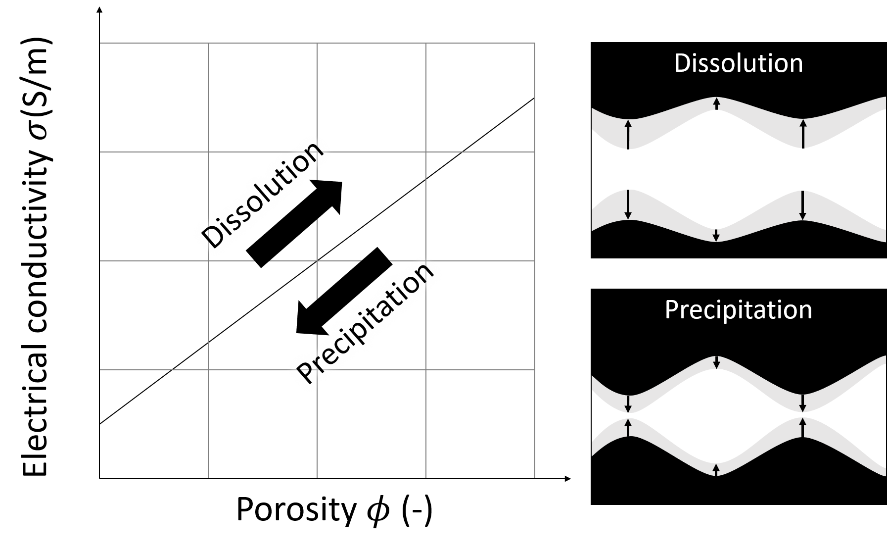
Graphical abstract: a new electrical conductivity model taking into account the effect of dissolution and precipitation on the pore shape at the REV scale through a fractal-based upscaling procedure.

1 Introduction

Carbonates represent a large part of the sedimentary rocks covering the Earth and carbonate aquifers store a large part of fresh water, which is a key resource for society needs. Karst aquifers are extremely complex systems because of the important chemical interactions between rock matrix and water, leading to strong chemical processes such as dissolution and precipitation. Studying these environments can benefit from the use of non-invasive tools such as the ones propose in hydrogeophysics to monitor flow and transport quantitatively (e.g., Hubbard and Linde, 2011; Binley et al., 2015).

Among the geophysical methods used for hydrological purposes in carbonate formations, electrical and electromagnetic methods have already shown their usefulness and are increasingly used (e.g., Chalikakis et al., 2011; Revil et al., 2012; Binley et al., 2015). Electrical methods, such as direct current (DC) resistivity and induced polarization (IP), involve acquisitions with flexible configurations of electrodes in galvanic or capacitive contact with the subsurface (Hubbard and Linde, 2011). These methods are increasingly used in different approaches to cover a larger field of applications: from samples measurements in the lab (e.g., Wu et al., 2010), to measurements in one or between several boreholes (e.g., Daily et al., 1992) and 3D or 4D monitoring with time-lapse imaging or with permanent surveys (e.g., Watlet et al., 2018; Saneiyan et al., 2019; Mary et al., 2020). Geophysical methods based on electromagnetic induction (EMI) consist in the deployment of electromagnetic coils in which an electric current of varying frequency is injected. Depending on the frequency range, the distance, and size of the coils for injection and reception, the depth of investigation can be highly variable (Reynolds, 1998). As for the electrical methods, EMI based methods can be deployed from the ground surface, in boreholes, and in an airborne manner (e.g., Paine, 2003).

These methods enable to determine the spatial distribution of the electrical conductivity in the subsurface. They are, hence, very useful in karst-system to detect the emergence of a sinkhole, to identify infiltration area, or to map ghost-rock features (e.g., Jardani et al., 2006; Chalikakis et al., 2011; Kaufmann and Deceuster, 2014; Watlet et al., 2018). The electrical conductivity can then be related to properties of interest for hydrogeological characterization through the use of accurate petrophysical relationships (Binley and Kemna, 2005). In recent works, electrical conductivity models are used to characterize chemical processes between rock matrix and pore water such as dissolution and precipitation (e.g., Leroy et al., 2017; Niu and Zhang, 2019). Indeed, geoelectrical measurements are an efficient proxy to describe pore space geometry (e.g., Garing et al., 2014; Jougnot et al., 2018) and transport properties (e.g., Jougnot et al., 2009, 2010; Hamamoto et al., 2010; Maineult et al., 2018).

The electrical conductivity $\sigma$ (S/m) of a water saturated porous medium (e.g., carbonate rocks) is a petrophysical property related to electrical conduction in the electrolyte through the transport of charges by ions. Then, $\sigma$ is linked to pore fluid electrical conductivity $\sigma_{w}$ (S/m) and to porous medium microstructural properties such as porosity $\phi$ (-), pore geometry, and surface roughness. Archie (1942) proposed a widely used empirical relationship for clean (clay-free) porous media that links $\sigma$ and $\sigma_{w}$ to $\phi$ as follows

$$\sigma\leavevmode\nobreak\ =\leavevmode\nobreak\ \sigma_{w}\leavevmode\nobreak\ \phi^{m},$$ (1)

where $m$ (-) is the cementation exponent, defined between 1.3 and 4.4 for unconsolidated samples and for most of well-connected sedimentary rocks (e.g., Friedman, 2005). For low pore water conductivity, porous medium electrical conductivity can also depend on a second mechanism, which can be described by the surface conductivity term $\sigma_{s}$ (S/m). This contribution to the overall rock electrical conductivity is caused by the presence of charged surface sites on the minerals. This causes the development of the so-called electrical double layer (EDL) with counterions (i.e., ions of the opposite charges) distributed in the Stern layer and the diffuse layer (Hunter, 1981; Chelidze and Gueguen, 1999; Leroy and Revil, 2004). Groundwater in carbonate reservoirs typically presents a conductivity comprised between 3.0$\times$10^-2 S/m and 8.0$\times$10^-2 S/m (e.g., Liñán Baena et al., 2009; Meyerhoff et al., 2014; Jeannin et al., 2016), while carbonate rich rocks surface conductivity can range from 2.9$\times$10^-4 S/m to 1.7$\times$10^-2 S/m depending on the amount of clay (Guichet et al., 2006; Li et al., 2016; Soueid Ahmed et al., 2020). Thus, for the study of dissolution and precipitation of water saturated carbonate rocks at standard values of $\sigma_{w}$, the surface conductivity is generally low and can be neglected (e.g., Cherubini et al., 2019). The small surface conductivity can nevertheless be considered as a parallel conductivity with an adjustable value (e.g., Waxman and Smits, 1968; Weller et al., 1958; Revil et al., 2014):

$$\sigma\leavevmode\nobreak\ =\leavevmode\nobreak\ \frac{1}{F}\leavevmode\nobreak\ \sigma_{w}\leavevmode\nobreak\ +\leavevmode\nobreak\ \sigma_{s}.$$ (2)

The formation factor $F$ (-) is thus assessed using a petrophysical law. Besides, since the late 1950’s many models linking $\sigma$ to $\sigma_{w}$ were developed. Most of these relationships have been obtained from the effective medium theory (e.g., Pride, 1994; Bussian, 1983; Revil et al., 1998; Ellis et al., 2010), volume averaging (e.g., Linde et al., 2006; Revil and Linde, 2006), the percolation theory (e.g., Broadbent and Hammersley, 1957; Hunt et al., 2014), or the cylindrical tube model (e.g., Pfannkuch, 1972; Kennedy and Herrick, 2012). More recently, the use of fractal theory (e.g., Yu and Li, 2001; Mandelbrot, 2004) of pore size has shown good results to describe petrophysical properties among which the electrical conductivity (e.g., Guarracino and Jougnot, 2018; Thanh et al., 2019). Meanwhile, several models have been developed to study macroscopic transport properties and chemical reactions by describing the porous matrix microscale geometry (e.g., Reis and Acock, 1994; Guarracino et al., 2014; Niu and Zhang, 2019) and theoretical petrophysical models of electrical conductivity have been derived to relate the pore structure to transport parameters (e.g., Johnson et al., 1986; Revil and Cathles, 1999; Glover et al., 2006).

Permeability prediction from electrical measurements is the subject of various research studies and these models often rely on petrophysical parameters such as the tortuosity (e.g., Revil et al., 1998; Niu and Zhang, 2019). Moreover, the use of models such as Archie (1942) and Carman (1939) to relate the formation factor, the porosity, and the permeability is reasonable for simple porous media such as unconsolidated packs with spherical grains, but it is less reliable for real rock samples or to study the effect of dissolution and precipitation processes. The aim of the present study is to develop a petrophysical model based on micro structural parameters, such as the tortuosity, the constrictivity (i.e., parameter which is related to bottleneck effect in pores, described by Holzer et al., 2013), and the Johnson length (e.g., Johnson et al., 1986; Bernabé and Maineult, 2015), to express the electrical conductivity and to evaluate the role of pore structure.

The present manuscript is divided into three parts. We first develop equations to describe the electrical conductivity of a porous medium with pores defined as tortuous capillaries that follow a fractal size distribution and presenting sinusoidal variations of their aperture. Then, the model is linked to other transport parameters such as permeability and ionic diffusion coefficient. In the second part, we test the model sensitivity and we compare its performance with Thanh et al. (2019) fractal model. In the third part, we confront the model to datasets presenting an increasing complexity: first data come from synthetic unconsolidated samples, then they are taken from natural rock samples with a growing pore space intricacy. Finally, we analyze the model response to numerical simulations of dissolution and precipitation, highlighting its interest as a monitoring tool for such critical processes.

2 Theoretical developments

Based on the approach of Guarracino et al. (2014), we propose a model assuming a porous medium represented as a fractal distribution of equivalent tortuous capillaries in a cylindrical representative elementary volume (REV) with a radius $R$ (m) and a length $L$ (m) (Fig. 1a). In this model, the surface conductivity $\sigma_{s}$ is neglected ($\sigma_{s}\xrightarrow{}0$).

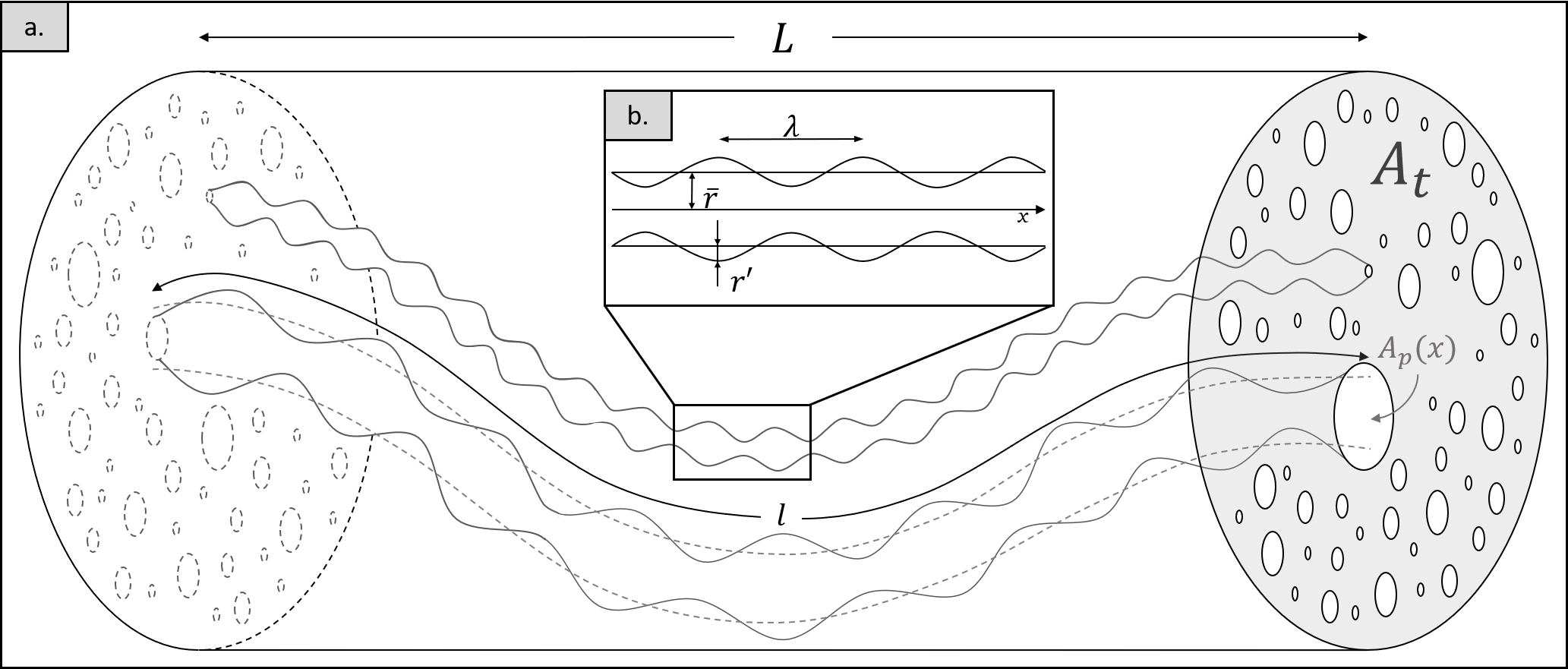
Figure 1: (a) The porous rock model is composed of a large number of sinusoidal and tortuous capillaries in the cylindrical representative elementary volume (REV). All the capillaries have the same tortuous length $l$ (m) and their radii follow a fractal distribution. (b) The considered pore geometry corresponds to the one from Guarracino et al. (2014): $\mathrm{bar}{r}$ is the average pore radius (m) while $r^{\prime}$ is the amplitude of the sinusoidal fluctuation (m), and $\lambda$ is the wavelength (m).

2.1 Pore scale

2.1.1 Pore geometry

The porous medium is conceptualized as an equivalent bundle of capillaries. As presented in Fig. 1b, each tortuous pore present a varying radius $r(x)$ (m) defined with the following sinusoidal expression,

$$r(x)\leavevmode\nobreak\ =\leavevmode\nobreak\ \mathrm{bar}{r}+r^{\prime}sin\left(\frac{2\pi}{\lambda}x\right)\leavevmode\nobreak\ =\leavevmode\nobreak\ \mathrm{bar}{r}\,\left(1+2a\leavevmode\nobreak\ sin\left(\frac{2\pi}{\lambda}x\right)\right),$$ (3)

where $\mathrm{bar}{r}$ is the average pore radius (m), $r^{\prime}$ the amplitude of the radius size fluctuation (m), and $\lambda$ is the wavelength (m). The parameter $a$ is the pore radius fluctuation ratio (-) defined by $a=r^{\prime}/2\mathrm{bar}{r}$, which values range from 0 to 0.5. Note that $a\leavevmode\nobreak\ =\leavevmode\nobreak\ 0$ corresponds to cylindrical pores ($r(x)\leavevmode\nobreak\ =\leavevmode\nobreak\ \mathrm{bar}{r}$), while $a\leavevmode\nobreak\ =\leavevmode\nobreak\ 0.5$ corresponds to periodically closed pores. For each pore we define the section area $A_{p}(x)\leavevmode\nobreak\ =\leavevmode\nobreak\ \pi r(x)^{2}$ (m²).

Most of the models found in the literature, and describing the porous medium with a fractal distribution, define a pore length scaling with pore radius (e.g., Yu and Cheng, 2002; Yu et al., 2003; Guarracino et al., 2014; Thanh et al., 2019). However, in this study we consider a constant tortuous length $l$ (m) for all the pores because it reduces the number of adjustable parameters while maintaining the model accuracy. This constant tortuosity value should be interpreted as an effective macroscopic value for all tube lengths. $l$ is the length taken at the center of the capillary. Thus, the tortuosity $\tau$ (-) is also a constant for all pores and is defined as

$$\tau\leavevmode\nobreak\ =\leavevmode\nobreak\ \frac{l}{L}.$$ (4)

In this case, the volume of a single pore $V_{p}(\mathrm{bar}{r})$ (m³) can be computed by integrating its section area $A_{p}(x)$ over the tortuous length $l$:

$$V_{p}(\mathrm{bar}{r})\leavevmode\nobreak\ =\leavevmode\nobreak\ \int_{0}^{l}{\pi r(x)^{2}dx}.$$ (5)

According to Eqs. (3) and (4), and assuming that $\lambda\ll l$, volume $V_{p}$ defined in Eq. (5) becomes

$$V_{p}(\mathrm{bar}{r})\leavevmode\nobreak\ =\leavevmode\nobreak\ \pi\mathrm{bar}{r}^{2}(1+2a^{2})\tau L.$$ (6)

2.1.2 Pore electrical conductivity

We express electrical properties at pore scale before obtaining them for the porous medium by upscaling, because the REV can be considered as an equivalent circuit of parallel conductances, when $\sigma_{s}$ is neglected. The electrical conductance $\Sigma_{pore}(\mathrm{bar}{r})$ ($S$) of a single sinusoidal pore is defined by

$$\Sigma_{pore}(\mathrm{bar}{r})\leavevmode\nobreak\ =\leavevmode\nobreak\ \left(\int_{0}^{l}{\frac{1}{\sigma_{w}\pi r(x)^{2}}dx}\right)^{-1},$$ (7)

where $\sigma_{w}$ (S/m) is the pore-water conductivity. Replacing Eq. (3) in Eq. (7) and assuming $\lambda\ll l$, the electrical conductance of a single pore can be expressed as

$$\Sigma_{pore}(\mathrm{bar}{r})\leavevmode\nobreak\ =\leavevmode\nobreak\ \frac{\sigma_{w}\pi\mathrm{bar}{r}^{2}(1-4a^{2})^{3/2}}{\tau L}.$$ (8)

Following Ohm’s law, the electric voltage $\Delta$V (V) between the edges of the capillary (0 and $l$) is defined as

$$\Delta V\leavevmode\nobreak\ =\leavevmode\nobreak\ -\frac{i(\mathrm{bar}{r})}{\Sigma_{pore}i(\mathrm{bar}{r})},$$ (9)

where $i(\mathrm{bar}{r})$ (A) is the electric current flowing through the pore that can be expressed as follows

$$i(\mathrm{bar}{r})\leavevmode\nobreak\ =\leavevmode\nobreak\ \frac{-\pi\leavevmode\nobreak\ \sigma_{w}\leavevmode\nobreak\ \mathrm{bar}{r}^{2}\leavevmode\nobreak\ (1-4a^{2})^{3/2}}{\tau\leavevmode\nobreak\ L}\leavevmode\nobreak\ \Delta V.$$ (10)

We, thus, define the contribution to the porous medium conductivity from a single pore $\sigma_{p}(\mathrm{bar}{r}$) (S/m) by multiplying the pore conductance with a geometric factor $f_{g}\leavevmode\nobreak\ =\leavevmode\nobreak\ \pi\leavevmode\nobreak\ R^{2}/L$ (m)

$$\sigma_{p}(\mathrm{bar}{r})\leavevmode\nobreak\ =\leavevmode\nobreak\ \frac{\Sigma_{pore}(\mathrm{bar}{r})}{f_{g}}\leavevmode\nobreak\ =\leavevmode\nobreak\ \frac{\mathrm{bar}{r}^{2}(1-4a^{2})^{3/2}\sigma_{w}}{\tau R^{2}}.$$ (11)

When $a\leavevmode\nobreak\ =\leavevmode\nobreak\ 0$, the expression of $\sigma_{p}(\mathrm{bar}{r})$ simplifies itself as in the case of cylindrical tortuous pores developed by Pfannkuch (1972).

2.2 Upscaling procedure using a fractal distribution

To obtain the electrical conductivity of the porous medium at the REV scale, we need a pore size distribution. We conceptualize the porous medium by a fractal distribution of capillaries according to the notations of Guarracino et al. (2014) and Thanh et al. (2019), based on the fractal theory for porous media (Tyler and Wheatcraft, 1990; Yu and Cheng, 2002)

$$N(\mathrm{bar}{r})\leavevmode\nobreak\ =\leavevmode\nobreak\ \left(\frac{\mathrm{bar}{r}_{max}}{\mathrm{bar}{r}}\right)^{D_{p}},$$ (12)

where $N$ (-) is the number of capillaries whose average radius are equal or larger than $\mathrm{bar}{r}$, $D_{p}$ (-) is the fractal dimension of pore size and $\mathrm{bar}{r}_{max}$ (m) is the maximum average radius of pores in the REV. Fractal distributions can be used to describe objects of different Euclidean dimensions (e.g., 1 dimension for a line, 2 dimensions for a surface, and 3 dimensions for a volume). In this study, the pore size distribution is considered as a fractal distribution of capillary sections on a plane (i.e., in 2 dimensions). Therefore, the fractal dimension $D_{p}$ is defined from 1 to 2 (among many other papers, see Yu and Cheng, 2002; Yu et al., 2003). Nevertheless, $D_{p}$ is a unique parameter for each porous medium as it strongly depends on the pore size distribution. Its impact has been quantified by Tyler and Wheatcraft (1990) with a porous medium defined as a Sierpinski carpet. From the pore size distribution defined in Equation (12), the total number of capillaries equals to

$$N_{tot}\leavevmode\nobreak\ =\leavevmode\nobreak\ \left(\frac{\mathrm{bar}{r}_{max}}{\mathrm{bar}{r}_{min}}\right)^{D_{p}},$$ (13)

with $\mathrm{bar}{r}_{min}$ (m) the minimum average radius. From Eq. (12), the number of radii lying between $\mathrm{bar}{r}$ and $\mathrm{bar}{r}+d\mathrm{bar}{r}$ is

$$-dN\leavevmode\nobreak\ =\leavevmode\nobreak\ D_{p}\leavevmode\nobreak\ \mathrm{bar}{r}_{max}^{\leavevmode\nobreak\ D_{p}}\leavevmode\nobreak\ \mathrm{bar}{r}^{\leavevmode\nobreak\ -D_{p}-1}\leavevmode\nobreak\ d\mathrm{bar}{r},$$ (14)

where $-dN$ (-) is the number of pores with an average radius comprised in the infinitesimal range between $\mathrm{bar}{r}$ and $\mathrm{bar}{r}+d\mathrm{bar}{r}$. The minus sign implies that the number of pores decreases when the average radius increases (Yu et al., 2003; Soldi et al., 2017; Thanh et al., 2019).

2.3 REV scale

In the present section, we present the macroscopic properties at the REV scale obtained from the upscaling procedure.

2.3.1 Porosity

We can express the porosity $\phi$ (-) of the REV by integrating the pore volume over the fractal distribution as follows

$$\phi\leavevmode\nobreak\ =\leavevmode\nobreak\ \frac{\int_{\mathrm{bar}{r}_{min}}^{\mathrm{bar}{r}_{max}}{V_{p}(\mathrm{bar}{r})}(-dN)}{\pi R^{2}L}.$$ (15)

Then, by replacing Eqs. (14) and (6) into Eq. (15), it yields to

$$\phi\leavevmode\nobreak\ =\leavevmode\nobreak\ \frac{(1+2a^{2})\tau D_{p}\mathrm{bar}{r}_{max}^{D_{p}}}{R^{2}(2-D_{p})}(\mathrm{bar}{r}_{max}^{2-D_{p}}-\mathrm{bar}{r}_{min}^{2-D_{p}}).$$ (16)

This expression requires $2-D_{p}>0$, which is always true (see Yu and Li, 2001). Note that this expression corresponds to the model of Guarracino et al. (2014) when the tortuosity is the same for all the capillary sizes.

2.3.2 Electrical conductivity

As defined in the Kirchhoff’s current law, the electric current of the REV, $I$ (A), is the sum of the electric currents of all the capillaries when the surface conductivity is neglected. It can be obtained by integrating the electric current of each pore:

$$I\leavevmode\nobreak\ =\leavevmode\nobreak\ \int_{\mathrm{bar}{r}_{min}}^{\mathrm{bar}{r}_{max}}i(\mathrm{bar}{r})(-dN).$$ (17)

According to Eqs. (4), (10), and (14), $I$ can be expressed as follows,

$$I\leavevmode\nobreak\ =\leavevmode\nobreak\ \frac{-\sigma_{w}\pi(1-4a^{2})^{3/2}D_{p}\mathrm{bar}{r}_{max}^{D_{p}}}{(2-D_{p})\tau L}\Delta V(\mathrm{bar}{r}_{max}^{2-D_{p}}-\mathrm{bar}{r}_{min}^{2-D_{p}}).$$ (18)

The Ohm’s law at the REV scale yields to

$$I\leavevmode\nobreak\ =\leavevmode\nobreak\ -\sigma^{REV}\pi R^{2}\frac{\Delta V}{L},$$ (19)

where $\sigma^{REV}$ is the electrical conductivity of the REV (S/m). By combining Eqs. (18) and (19), $\sigma^{REV}$ is expressed as

$$\sigma^{REV}\leavevmode\nobreak\ =\leavevmode\nobreak\ \frac{\sigma_{w}D_{p}\mathrm{bar}{r}^{D_{p}}_{max}(1-4a^{2})^{3/2}}{R^{2}\tau(2-D_{p})}(\mathrm{bar}{r}_{max}^{2-D_{p}}-\mathrm{bar}{r}_{min}^{2-D_{p}}).$$ (20)

Finally, substituting Eq. (16) into Eq. (20) yields to

$$\sigma^{REV}\leavevmode\nobreak\ =\leavevmode\nobreak\ \frac{\sigma_{w}\phi(1-4a^{2})^{3/2}}{\tau^{2}(1+2a^{2})}.$$ (21)

Note that if $a$ = 0 and $\tau$ = 1, Eq. (21) becomes $\sigma^{REV}\leavevmode\nobreak\ =\leavevmode\nobreak\ \sigma_{w}\phi$, which is the expression of Archie’s law for $m$ = 1 where the porous medium is composed of a bundle of straight capillaries with no tortuosity (see Clennell, 1997).

The electrical conductivity can be rewritten depending on the tortuosity $\tau$ and on the constrictivity $f$ (-) as

$$\sigma^{REV}\leavevmode\nobreak\ =\leavevmode\nobreak\ \frac{\sigma_{w}\phi f}{\tau^{2}}.$$ (22)

The constrictivity $f$ is thus defined as

$$f\leavevmode\nobreak\ =\leavevmode\nobreak\ \frac{(1-4a^{2})^{3/2}}{(1+2a^{2})}.$$ (23)

The above equation highlights that the pore fluctuation ratio $a$ plays the role of the constriction factor defined by Petersen (1958). Constrictivity $f$ ranges between 0 (e.g., for trapped pores) and 1 (e.g., for cylindrical pores with constant radius). As for the tortuosity $\tau$, there is no suitable method to determine constrictivity value directly from core samples, but only some mathematical expressions for ideal simplified geometries (see Holzer et al., 2013, for a review). Therefore, very high tortuosity values (e.g., Niu and Zhang, 2019) must be due to that in most studies the bottleneck effect is not considered.

2.3.3 Formation factor

The model from Archie (1942) links the rock electrical conductivity to the pore water conductivity and the porosity with the cementation exponent, which is an empirical parameter. Kennedy and Herrick (2012) propose to analyze electrical conductivity data using a physics-based model, which conceptualizes the porous medium with pore throats and pore bodies as in this study and defines the electrical conductivity as follows,

$$\sigma^{REV}\leavevmode\nobreak\ =\leavevmode\nobreak\ G\sigma_{w}\phi,$$ (24)

where $G$ (-) is an explicit geometrical factor defined between 0 and 1. According to our models G can be expressed by

$$G\leavevmode\nobreak\ =\leavevmode\nobreak\ \frac{(1-4a^{2})^{3/2}}{\tau^{2}(1+2a^{2})}\leavevmode\nobreak\ =\leavevmode\nobreak\ \frac{f}{\tau^{2}}.$$ (25)

This geometrical factor can be called the connectedness (Glover, 2015), while the formation factor $F$ (-) is defined by

$$F\leavevmode\nobreak\ =\leavevmode\nobreak\ \frac{\sigma_{w}}{\sigma^{REV}}.$$ (26)

Substituting Eq. (21) into Eq. (26) yields to

$$F\leavevmode\nobreak\ =\leavevmode\nobreak\ \frac{\tau^{2}(1+2a^{2})}{\phi(1-4a^{2})^{3/2}}\leavevmode\nobreak\ =\leavevmode\nobreak\ \frac{\tau^{2}}{\phi f}.$$ (27)

The formation factor $F$ can also be related to the connectedness $G$ as $F\leavevmode\nobreak\ =\leavevmode\nobreak\ 1/\phi G$.

2.4 Evolution of the petrophysical parameters

The formation factor defined by Eq. (27) depends linearly with the inverse of porosity (1/$\phi$). However, the petrophysical parameters $a$ and $\tau$ may be dependent on porosity for certain types of rocks or during dissolution or precipitation processes. In these cases, the formation factor will show a non-linear dependence with 1/$\phi$ and can be expressed in general as

$$F(\phi)=\frac{\tau(\phi)^{2}(1+2a(\phi)^{2})}{\phi(1-4a(\phi)^{2})^{3/2}}.$$ (28)

In section 4.2, we test our model against different datasets from literature using logarithmic laws for the dependence of petrophysical parameters $a(\phi)$ and $\tau(\phi)$ with porosity following existing models from the literature (see Ghanbarian et al., 2013, for a review about the tortuosity). Thus, we define $a(\phi)$ and $\tau(\phi)$ as

$$a(\phi)\leavevmode\nobreak\ =\leavevmode\nobreak\ -P_{a}\log(\phi)$$ (29)

and

$$\tau(\phi)\leavevmode\nobreak\ =\leavevmode\nobreak\ 1-P_{\tau}\log(\phi),$$ (30)

where $P_{a}$ and $P_{\tau}$ are empirical parameters. Note that 0 and 1 (i.e., first terms in Eqs. (29) and (30), respectively) correspond to the minimum values reached by $a(\phi)$ and $\tau(\phi)$ when $\phi$ = 1. Expressing tortuosity as a logarithmic function of porosity has already proven its effectiveness in the literature (Comiti and Renaud, 1989; Ghanbarian et al., 2013; Zhang et al., 2020). However, this is, to the best of our knowledge, the first attempt to propose a constrictivity model as a function of porosity. Then, by replacing Eqs. (29) and (30) in Eq. (28), the expression of the proposed model for the formation factor $F$ becomes

$$F(\phi)\leavevmode\nobreak\ =\leavevmode\nobreak\ \frac{\left[1-P_{\tau}\log(\phi)\right]^{2}\left(1+2\left[P_{a}\log(\phi)\right]^{2}\right)}{\phi\left(1-4\left[P_{a}\log(\phi)\right]^{2}\right)^{3/2}}.$$ (31)

Note that the model parameters from Thanh et al. (2019), another porous medium description following a fractal distribution of pores, also present logarithmic dependencies with the porosity $\phi$.

2.5 Electrical conductivity and transport parameters

2.5.1 From electrical conductivity to permeability

The electrical conductivity is a useful geophysical property to describe the pore space geometry. Here we propose to express the permeability as a function of the electrical conductivity using our model.

At pore scale, Sisavath et al. (2001) propose the following expression for the flow rate $Q_{p}(\mathrm{bar}{r})$ (m³/s) in a single capillary:

$$Q_{p}(\mathrm{bar}{r})\leavevmode\nobreak\ =\leavevmode\nobreak\ \frac{\pi}{8}\leavevmode\nobreak\ \frac{\rho g}{\mu}\leavevmode\nobreak\ \frac{\Delta h}{l}\leavevmode\nobreak\ \left[\int_{0}^{l}\frac{1}{r^{4}(x)}dx\right]^{-1}.$$ (32)

where $\rho$ is the water density (kg/m³), $g$ is the standard gravity acceleration (m/s²), $\mu$ is the water viscosity (Pa.s) and $\Delta h$ is the hydraulic head across the REV (m). Substituting Eq. (3) in Eq. (32) and assuming $\lambda\ll l$, it yields:

$$Q_{p}(\mathrm{bar}{r})\leavevmode\nobreak\ =\leavevmode\nobreak\ \frac{\pi}{8}\leavevmode\nobreak\ \frac{\rho g}{\mu}\leavevmode\nobreak\ \frac{\Delta h}{\tau L}\leavevmode\nobreak\ \mathrm{bar}{r}^{4}\leavevmode\nobreak\ (1-4a^{2})^{3/2}.$$ (33)

Then, the total volumetric flow rate $Q^{REV}$ (m³/s) is obtained by integrating Eq. (33) over all capillaries (i.e., at the REV scale)

$$\begin{array}[]{r c l}Q^{REV}&=&\int_{\mathrm{bar}{r}_{min}}^{\mathrm{bar}{r}_{max}}Q_{p}(\mathrm{bar}{r})(-dN)\\ &=&\frac{\rho g(1-4a^{2})^{3/2}D_{p}\mathrm{bar}{r}_{max}^{D_{p}}\pi\Delta h}{8\mu(4-D_{p})\tau L}(\mathrm{bar}{r}_{max}^{\leavevmode\nobreak\ 4-D_{p}}-\mathrm{bar}{r}_{min}^{\leavevmode\nobreak\ 4-D_{p}}).\end{array}$$ (34)

Based on Darcy’s law for saturated porous media, the total volumetric flow rate can be expressed as

$$Q^{REV}\leavevmode\nobreak\ =\leavevmode\nobreak\ \pi R^{2}\frac{\rho g}{\mu}k^{REV}\frac{\Delta h}{L},$$ (35)

where $k^{REV}$ is the REV permeability (m²). Then, combining Eqs. (34) and (35) it yields to

$$k^{REV}\leavevmode\nobreak\ =\leavevmode\nobreak\ \frac{(1-4a^{2})^{3/2}D_{p}\mathrm{bar}{r}_{max}^{D_{p}}}{8R^{2}(4-D_{p})\tau}(\mathrm{bar}{r}_{max}^{\leavevmode\nobreak\ 4-D_{p}}-\mathrm{bar}{r}_{min}^{\leavevmode\nobreak\ 4-D_{p}}).$$ (36)

Considering $\mathrm{bar}{r}_{min}\ll\mathrm{bar}{r}_{max}$, Eq. (36) can be simplified as

$$k^{REV}\leavevmode\nobreak\ =\leavevmode\nobreak\ \frac{(1-4a^{2})^{3/2}D_{p}\mathrm{bar}{r}_{max}^{4}}{8R^{2}(4-D_{p})\tau}.$$ (37)

Using the same simplification on Eq. (16), the expression of porosity becomes

$$\phi\leavevmode\nobreak\ =\leavevmode\nobreak\ \frac{(1+2a^{2})\tau D_{p}\mathrm{bar}{r}_{max}^{2}}{R^{2}(2-D_{p})}.$$ (38)

Then, combining Eqs. (37) and (38) yields to

$$k^{REV}\leavevmode\nobreak\ =\leavevmode\nobreak\ \frac{2-D_{p}}{4-D_{p}}\leavevmode\nobreak\ \frac{(1-4a^{2})^{3/2}}{1+2a^{2}}\leavevmode\nobreak\ \frac{\mathrm{bar}{r}_{max}^{2}}{8\tau^{2}}\phi.$$ (39)

Finally, the combination of Eqs. (27) and (39) leads to

$$k^{REV}\leavevmode\nobreak\ =\leavevmode\nobreak\ \frac{2-D_{p}}{4-D_{p}}\leavevmode\nobreak\ \frac{\mathrm{bar}{r}_{max}^{2}}{8F}.$$ (40)

Note that Eq. (40) relates permeability to electrical conductivity through the formation factor (see Eq. (26)).

This expression can be linked to the model of Johnson et al. (1986)

$$k^{REV}\leavevmode\nobreak\ =\leavevmode\nobreak\ \frac{\Lambda^{2}}{8F},$$ (41)

where $\Lambda$ (also known as the Johnson length) is a characteristic pore size (m) of dynamically connected pores (Banavar and Schwartz, 1987; Ghanbarian, 2020). Some authors proposed theoretical relationships to determine this characteristic length $\Lambda$. While Revil and Cathles (1999) or Glover et al. (2006) link it to the average grain diameter, some other publications work on the determination of $\Lambda$ assuming a porous medium composed of cylindrical pores (e.g., Banavar and Johnson, 1987; Niu and Zhang, 2019). Considering the proposed model, $\Lambda$ can therefore be written as follows

$$\Lambda\leavevmode\nobreak\ =\leavevmode\nobreak\ \sqrt{\frac{2-D_{p}}{4-D_{p}}}\leavevmode\nobreak\ \mathrm{bar}{r}_{max}.$$ (42)

2.5.2 From electrical conductivity to ionic diffusion coefficient

Ionic diffusion can be described at REV scale by the Fick’s law (Fick, 1995)

$$J_{t}\leavevmode\nobreak\ =\leavevmode\nobreak\ D_{eff}\,\pi R^{2}\frac{\Delta c}{L},$$ (43)

where $J_{t}$ (mol/s) is the diffusive mass flow rate, $D_{eff}$ (m²/s) is the effective diffusion coefficient, and $\Delta c$ (mol/m³) is the solute concentration difference between the REV edges. Guarracino et al. (2014) propose to express $D_{eff}$ as a function of the tortuosity, which, in their model, depends on the capillary size. In our model, we consider that the tortuosity is constant, thus by reproducing the same development proposed by Guarracino et al. (2014) we obtain

$$D_{eff}\leavevmode\nobreak\ =\leavevmode\nobreak\ D_{w}\frac{(1-4a^{2})^{3/2}\phi}{(1-2a^{2})\tau^{2}},$$ (44)

which can be simplified as

$$D_{eff}\leavevmode\nobreak\ =\leavevmode\nobreak\ D_{w}\frac{f\phi}{\tau^{2}}.$$ (45)

This last expression of $D_{eff}$ as a function of the tortuosity $\tau$ and the constrictivity $f$, allows to retrieve the same equation as Van Brakel and Heertjes (1974) with both the effect of the tortuosity and the constrictivity. Replacing Eq. (27) in Eq. (45) yields to

$$D_{eff}\leavevmode\nobreak\ =\leavevmode\nobreak\ \frac{D_{w}}{F},$$ (46)

which implies

$$F\leavevmode\nobreak\ =\leavevmode\nobreak\ \frac{\sigma_{w}}{\sigma^{REV}}\leavevmode\nobreak\ =\leavevmode\nobreak\ \frac{D_{w}}{D_{eff}}.$$ (47)

This result has already been demonstrated by Kyi and Batchelor (1994) and Jougnot et al. (2009), among others. It means that the formation factor can be used for both electrical conductivity or diffuse properties. This point is consistent with the fact that Ohm and Fick laws are diffusion equations, where the transport of ions take place in the same pore space. The difference lies in the fact that ionic conduction and ionic diffusion consider the electric potential gradient and the ionic concentration gradient, respectively.

3 Model analysis and evaluation

Our model expresses the evolution of the formation factor $F$ as a function of the porosity $\phi$, the tortuosity $\tau$ and the constrictivity through the pore radius fluctuation ratio $a$ (Eq. (27)). Here we explore wide ranges of values for $a$ and $\tau$ to quantify their influence on the formation factor $F$ (Fig. 2) and compare our model with the model from Thanh et al. (2019), for the fractal dimension of the tortuosity $D_{\tau}$ = 1, to appreciate the contribution of the constrictivity to the porous medium description. Figs. 2a and 2b show variations of $F$ as a function of the porosity $\phi$ when only $a$ or $\tau$ varies. On Fig. 2a, parameter $a$ varies from 0 to 0.49 and tortuosity $\tau\leavevmode\nobreak\ =\leavevmode\nobreak\ 5.0$. We test the case of a constant pore aperture when $a$ = 0, but we do not reach $a$ = 0.5 because this means that the pores are periodically closed (see the definition of $a$ in section 2.1.1), and this corresponds to an infinitely resistive rock only made of non-connected porosity. On Fig. 2b tortuosity $\tau$ varies from 1 to 20 and parameter $a\leavevmode\nobreak\ =\leavevmode\nobreak\ 0.1$. $\tau$ = 1 implies straight pores (i.e., $l=L$). Fig. 2c present variations of $F$ as a function of the tortuosity $\tau$ for different values of $a$ and a fixed porosity $\phi\leavevmode\nobreak\ =\leavevmode\nobreak\ 0.4$. Fig. 2d is the density plot of $\log_{10}(F)$ for a range of values of $a$ and $\tau$ and with a fixed porosity value $\phi\leavevmode\nobreak\ =\leavevmode\nobreak\ 0.4$.

Figure 2: (a) Effect of the pore radius fluctuation ratio $a$ on the formation factor $F$, represented as a function of the porosity $\phi$. $a$ varies from 0 to 0.49, while the tortuosity $\tau$ = 5. (b) Effect of the tortuosity $\tau$ on the formation factor $F$, represented as a function of the porosity $\phi$. $\tau$ varies from 1 to 20, while the pore radius fluctuation ratio $a$ = 0.1. (c) Effect of the pore radius fluctuation ratio $a$ on the formation factor $F$, represented as a function of the tortuosity $\tau$. $a$ varies from 0 to 0.49, while the porosity $\phi$ = 0.4. (d) Comparison of the effect of parameters $a$ and $\tau$ on the formation factor $F$ for a constant porosity $\phi$ = 0.4.

From the analysis of Figs. 2a and 2b, one can note that the formation factor decreases when porosity increases. This was expected because more the water saturated medium is porous, more its electrical conductivity is close to pore water electrical conductivity. Furthermore, we observe that both parameters $a$ and $\tau$ have a strong effect on formation factor variation ranges. Indeed, $F(\phi)$ curve can be shifted by more than 3 orders of magnitude with variations of $a$ or $\tau$ and, as expected, the formation factor increases when $\tau$ or $a$ increases. Indeed, when these parameters increase, the porous medium becomes more complex: the increase of parameter $a$ means that periodical aperture of capillaries decreases (i.e., more constrictivity), while the increase of $\tau$ means that pores become more tortuous (i.e., more tortuosity). Besides, for $a$ close to 0 (i.e., without aperture variation), curves from Thanh et al. (2019) model are similar with the curves from our model. This is consistent with the fact that Thanh et al. (2019) also conceptualize the porous media as a fractal distribution of capillaries. However, when $a$ increases, the curves explore very different ranges of $F$ values (Figs. 2a and 2c). The density plot presented on Fig. 2d compares the effect of $a$ and $\tau$ variations for a constant porosity ($\phi\leavevmode\nobreak\ =\leavevmode\nobreak\ 0.4$). It appears that for a fixed value of $\tau$, variations of $a$ have a low effect on log of $F$ values. On the contrary, variations of $\tau$ for one value of $a$ have stronger effect on log of $F$ ranges. However it should be noted that this representation can be biased because value ranges of $a$ and $\tau$ are very different. Thus, it is difficult to asses if the tortuosity $\tau$ has really much more effect on formation factor than parameter $a$. Nevertheless, it has the advantage to represent the combined effect of $a$ and $\tau$ on the formation factor.

4 Results and discussion

To assess the performance of the proposed model, we compare predicted values to datasets from the literature. References are listed in Table 1 and ordered with a growing complexity. Indeed, data from Friedman and Robinson (2002) and Bolève et al. (2007) are taken from experiments made on unconsolidated medium. Then, Garing et al. (2014), Revil et al. (2014), and Cherubini et al. (2019) studied natural consolidated samples from carbonate rocks and sandstone samples. Finally, Niu and Zhang (2019) present numerical but dynamic data under dissolution and precipitation conditions.

Table 1: Parameters of the proposed model compared to several datasets from different sources. $\sigma_{s}$ is the surface conductivity (S/m) used for several comparisons out of our model application range, that is when the surface conductivity cannot be neglected, using Eq. (2). The model parameters are adjusted with a Monte-Carlo approach, except for $a$ in Niu and Zhang (2019) dataset, where $a$ is adjusted with the least square method. $\epsilon$ is the cumulative error computed in percentage, called the mean absolute percentage error (MAPE).

Sample	$a$	$\tau$	$\sigma_{s}$	$\epsilon$	Studied	Source
			(S/m)	(%)	function
S1a	0.004	1.035	2.25 $\times 10^{-4}$	7.78	$\sigma(\sigma_{w})$	Bolève et al. (2007)
S2	0.008	1.062	1.45 $\times 10^{-4}$	7.47
S3	0.006	1.050	0.80 $\times 10^{-4}$	7.09
S4	0.006	1.051	0.50 $\times 10^{-4}$	9.21
S5	0.012	1.093	0.25 $\times 10^{-4}$	10.22
S6	0.008	1.062	0.60 $\times 10^{-4}$	9.21
Glass	0.022	1.174	-	0.32	$F(\phi)$	Friedman and Robinson (2002)
Sand	0.026	1.212	-	0.60
Tuff	0.020	1.159	-	1.63
FS$\,{}^{a}$	0.146 - 0.309	1.365 - 1.773	-	22.62	$F(\phi)$	Revil et al. (2014)
L1, L2	0.113	1.901	7.24 $\times 10^{-4}$	9.24	$\sigma(\sigma_{w})$	Cherubini et al. (2019)
Inter	0.077 - 0.217	1.846 - 3.399	-	26.67	$F(\phi)$	Garing et al. (2014)
Multi	0.172 - 0.345	1.915 - 2.839	-	9.64
Vuggy	0.068 - 0.109	5.632 - 8.411	-	19.68
D.T.lim$\,{}^{b}$	0.078 - 0.393	1.786	-	0.05	$F(\phi)$	Niu and Zhang (2019)
D.R.lim$\,{}^{c}$	0.315 - 0.393	1.786	-	0.08
P.T.lim$\,{}^{d}$	0.167 - 0.466	1.335	-	0.12
P.R.lim$\,{}^{e}$	0.160 - 0.309	1.320	-	0.04
a FS: Fontainebleau sandstones
b D.T.lim: Dissolution transport-limited
c D.R.lim: Dissolution reaction-limited
d P.T.lim: Precipitation transport-limited
e P.R.lim: Precipitation reaction-limited

For each dataset, the adjusted parameters of the proposed model are listed in Table 1. Values have been determined using a Monte-Carlo inversion of Eqs. (21) and (27) which express the porous medium electrical conductivity $\sigma^{REV}$ as a function of the pore water conductivity $\sigma_{w}$ and the formation factor $F$ as a function of the porosity $\phi$, respectively. An additional term $\sigma_{s}$ for the surface conductivity (S/m) is used to fit the data out of the application range of the proposed model. That is for low values of pore-water conductivity, when the surface conductivity cannot be neglected. As the proposed model is intended to be mostly used on carbonate rocks, which are known to have low surface conductivity, this physical parameter has not been taken into account in the theoretical development of the expression of the electrical conductivity of the porous medium. However, it can be added considering a parallel model (e.g., Waxman and Smits, 1968; Börner and Schön, 1991):

$$\sigma^{REV}\leavevmode\nobreak\ =\leavevmode\nobreak\ \frac{1}{F}\sigma_{w}+\sigma_{s}.$$ (48)

A more advanced approach of parallel model is proposed by Thanh et al. (2019) including the contribution of the surface conductance in the overall capillary bundle electrical conductivity.

Table 1 lists also the computed error $\epsilon$ of the adjusted model. In statistics $\epsilon$ is called the mean absolute percentage error (MAPE). It is expressed in percent and defined as follow:

$$\epsilon\leavevmode\nobreak\ =\leavevmode\nobreak\ \frac{1}{N^{d}}\left(\sum^{N^{d}}_{i=1}\left|\frac{P^{m}_{i}-P^{d}_{i}}{P^{d}_{i}}\right|\right)\times 100,$$ (49)

where $N^{d}$, $P^{d}$, and $P^{m}$ refer to the number of data, the electrical property from data, and the electrical property from the model, respectively. This type of error has been chosen to compare the ability of the model to reproduce the experimental values for all the datasets even if they are expressed as $\sigma^{REV}(\sigma_{w})$ or as $F(\phi)$.

4.1 Testing the model on unconsolidated media

The proposed model is first confronted to datasets from Friedman and Robinson (2002) and Bolève et al. (2007) obtained for unconsolidated samples. In these tests, only one set of parameters $a$, $\tau$, and $\sigma_{s}$ (when needed) is adjusted to fit with each dataset.

Bolève et al. (2007) measured the electrical conductivity of glass beads samples for different values of the pore water conductivity $\sigma_{w}$ from $10^{-4}$ S/m to $10^{-1}$ S/m on S1a, S2, S3, S4, S5, and S6 (see Fig. 3). For all samples, Bolève et al. (2007) reported a constant porosity of 40 % while grain diameters are comprised between $56\text{\,}\mathrm{\SIUnitSymbolMicro m}$ for S1a and $3000\text{\,}\mathrm{\SIUnitSymbolMicro m}$ for S6 (see Fig. 3 for more details).

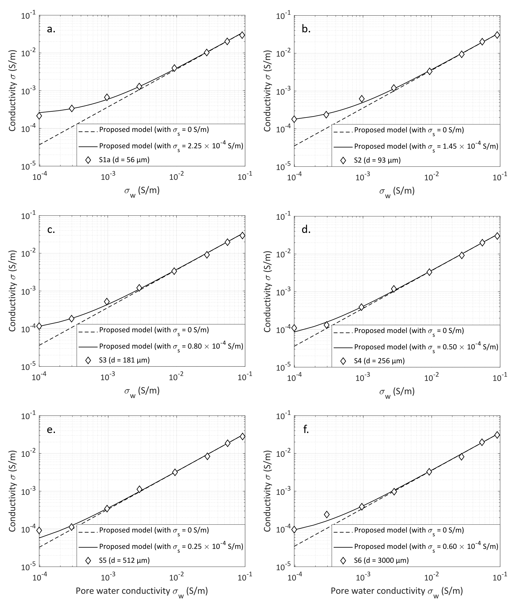
Figure 3: Electrical conductivity of different samples of glass beads (grains sizes are 56, 93, 181, 256, 512, and $3000\text{\,}\mathrm{\SIUnitSymbolMicro m}$ for samples S1a, S2, S3, S4, S5, and S6, respectively) versus the fluid electrical conductivity for a constant porosity $\phi\leavevmode\nobreak\ =\leavevmode\nobreak\ 40\leavevmode\nobreak\ \%$. The datasets are from Bolève et al. (2007) and best fit parameters are given in Table 1.

Table 1 shows that the adjusted model parameters $a$ and $\tau$ have rather similar values for all the samples from Bolève et al. (2007). This can be explained by the fact that all samples have the same pore geometry but scaled at different size. Indeed, for homogeneous samples of glass beads, the beads space arrangement is quite independent of the spheres size. Therefore the pore network of all samples presents similar properties such as tortuosity (see also the discussion in Guarracino and Jougnot, 2018) and constrictivity, which directly depends on parameters $a$ and $\tau$. Moreover, $a$ and $\tau$ are close to their minimum limits (i.e., $a$ = 0 and $\tau$ = 1). This is due to the simple pore space geometry created by samples made of homogeneous glass spheres. This explains the model good fit for straight capillaries (i.e., Thanh et al., 2019). However, it can be noticed that surface conductivity decreases while grain diameter increases. This is not a surprise considering that for the same volume, samples of smaller beads have a larger specific surface than samples of bigger beads (see, for example, the discussion in Glover and Déry, 2010).

Friedman and Robinson (2002) determined the formation factor $F$ for samples of glass beads, sand, and tuff grains with different values of porosity $\phi$ (see Fig. 4). As the model best fit is determined with a Monte Carlo approach, accepted models are also plotted on Fig. 4. The acceptance criterion is defined individually for each dataset and corresponds to a certain value of the MAPE $\epsilon$. For samples from Friedman and Robinson (2002), this criterion is fixed at $\epsilon<$ 1 or 2 %. These are low values, meaning a really good fit from the model.

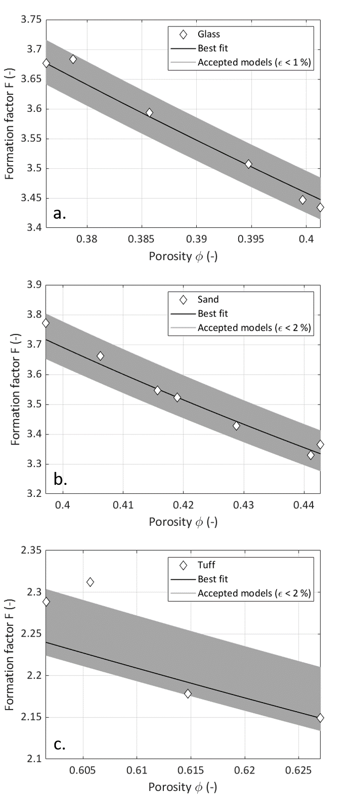
Figure 4: Formation factor of samples with different porosity values: (a) glass beads, (b) sand, and (c) tuff grains (Friedman and Robinson, 2002). The sets of adjusted model parameters $a$ and $\tau$ are given in Table 1.

We observe from Table 1 that $a$ and $\tau$ values are close to each other for all samples from Friedman and Robinson (2002). However, these parameters have higher values than for Bolève et al. (2007) dataset. This comes from the fact that some complexity is added in the dataset from Friedman and Robinson (2002). Indeed, the samples of Friedman and Robinson (2002) combine particles of different sizes. In this case, smaller grains can fill the voids left by bigger grains. This grains arrangement decreases the medium porosity but increases its tortuosity and constrictivity. Furthermore, sand and tuff grains have rougher surface and are less spherical than glass beads. This explains the misfit increase between data and model for glass, sand, and tuff samples (Friedman and Robinson, 2002). Nevertheless, even for tuff grains, the misfit between data and model is still very low compared to the computed MAPE from Bolève et al. (2007) samples. This is due to that for Bolève et al. (2007), a wide range of pore water conductivity values is explored and thus electrical properties vary much more (over 3 orders of magnitude) than in the case of Friedman and Robinson (2002).

4.2 Testing the model on consolidated rock samples

In this section, we test our model against datasets of Garing et al. (2014), Revil et al. (2014), and Cherubini et al. (2019). They study carbonate samples from the reef unit of Ses Sitjoles site (from Mallorca), Fontainebleau sandstones, and two Estaillades limestones (rodolith packstones), respectively.

Figure 5: (a) Formation factors of a set of Fontainebleau sandstones versus porosity (the dataset is from Revil et al., 2014). Model parameters are given in Table 1. (b) and (c) $a$ and $\tau$ are defined as logarithmic functions of the porosity $\phi$.

Revil et al. (2014) obtained a wide range of formation factor values for a large set of Fontainebleau sandstone core samples over a large range of porosity. We first test our model with constant values of $a$ and $\tau$, but we observed that the model could not fit data (see Fig. 5a). This can be explained by the fact that this dataset is composed of numerous sandstone samples presenting a wide range of porosity values (from 0.045 to 0.22). Therefore, we consider that the samples have distinct pore geometry which is describable by $a(\phi)$ and $\tau(\phi)$ distributions, presented in section 2.4 and plotted on Figs. 5b and 5c. We observe that parameters $a$ and $\tau$ logarithmic evolution with the porosity $\phi$ are physically plausible as lower porosity can reflect more complex medium geometries (i.e., more constrictive and more tortuous), described with higher values of $a$ and $\tau$. On Fig. 5a, we also plot the model from Thanh et al. (2019). Even if the curve presents a slope similar to dataset, it overestimates the formation factor.

Despite a quite wide dispersion of the formation factor data for the lowest porosities, it appears that the proposed model is well adjusted to the dataset. Indeed, the proposed model MAPE $\epsilon\leavevmode\nobreak\ =\leavevmode\nobreak\ 22.62\leavevmode\nobreak\$% (see Table 1), while $\epsilon\leavevmode\nobreak\ =\leavevmode\nobreak\ 89.63\leavevmode\nobreak\$% for the model from Thanh et al. (2019). Note that the relatively high MAPE value comes from the large spread of the formation factor values. Thus, it seems that taking into account the constrictivity of the porous medium in addition to the tortuosity highly improves modeling.

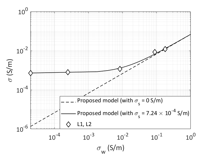
Figure 6: Electrical conductivity of two limestones (L₁ and L₂) versus water electrical conductivity. The dataset is from Cherubini et al. (2019) and model parameters are given in Table 1.

Fig. 6 shows the dependence of electrical conductivity with pore-water electrical conductivity for two limestone samples (named L1 and L2) from Cherubini et al. (2019). Table 1 shows that model parameters and surface conductivity values are larger than for the unconsolidated samples from Bolève et al. (2007) and Friedman and Robinson (2002). This is explained by the fact that natural rock samples can present a more complex geometry and larger specific surface area than glass beads samples. Cherubini et al. (2019) predict the surface electrical conductivity with the model from Revil et al. (2014). They obtain $\sigma_{s}\leavevmode\nobreak\ =\leavevmode\nobreak\ 7.0\times 10^{-4}$ S/m, which is very close to the value obtained in this study. Furthermore, the computed errors for the dataset of Bolève et al. (2007) and for these limestones are close to each other. This test illustrates that even for more complex porous media, the proposed model has still a good data resolution.

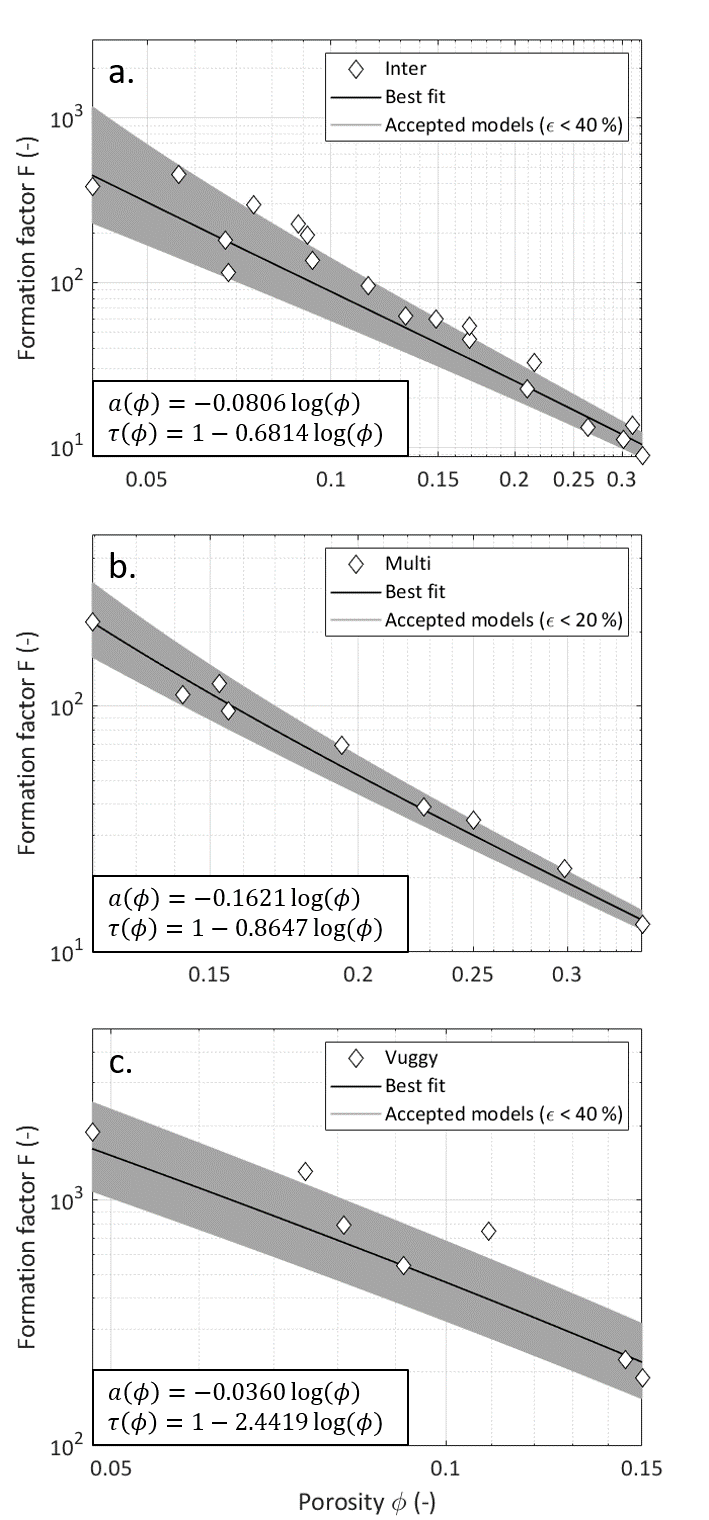
Figure 7: Formation factors of a set of carbonate rocks classified by pore types versus porosity. The dataset is from Garing et al. (2014). The model parameters are given in Table 1. The proposed model parameters are considered to be logarithmic functions of $\phi$. (a) “inter” stands for samples with intergranular pores (b) “multi” gathers samples with multiple porosity types: intergranular, moldic, and vuggy. (c) “vuggy” represents samples with vugular porosity.

Garing et al. (2014) conducted X-ray microtomography measurements on carbonate samples to classify them by pore types and thus they highlight three groups:

1. “Inter” samples present intergranular pores. This pore shape is quite comparable with sandstones porosity type.

2. “Multi” samples hold multiple porosity types: intergranular, moldic, and vugular. Microtomograms of “multi” samples show small but well connected pores. The analyze conducted by Garing et al. (2014) revealed that for samples with smaller porosity, pores are smaller on average, but still numerous and well connected, even for a reduced microporosity.

3. “Vuggy” samples possess vugular porosity. Microtomography highlights the presence of few vugs badly connected, which are less numerous for samples of lower porosity.

Fig. 7 presents the results of formation factor computation versus porosity. As for the dataset from Revil et al. (2014), the proposed model is adjusted using Eq. (31), which considers that model parameters are logarithmic functions of porosity. Despite some dispersion for “inter” and “vuggy” samples (i.e., the acceptance criterion $\epsilon<40\leavevmode\nobreak\$%), the model explains well the data for all porosity types and present low MAPE values (Table 1).

The analysis of parameters $P_{a}$ and $P_{\tau}$ reveals that they present consistent values for the different porosity types. Indeed, for “vuggy” samples, $P_{a}$ is small while $P_{\tau}$ is high (Fig. 7c). According to Eqs. (29) and (30), these values lead to low and high values for $a$ and $\tau$, respectively (Table 1), and this is consistent with the microtomography analysis from Garing et al. (2014). Indeed, since these samples present large vugs badly connected (i.e., few microporosity), the microstructure is very tortuous but pores are not constricted. Furthermore, for samples with lower porosity, vugs are still present in “vuggy” samples, but they are less numerous, which leads to a microstructure even more tortuous, but nearly as constrictive as for the more porous samples. Moreover, for “inter” and “multi” samples (Figs. 7a and 7b), $P_{a}$ and $P_{\tau}$ are closer in value to the parameters of the sandstone samples from Revil et al. (2014) than to the parameters of “vuggy” samples because they have, among other types for the “multi” samples, intergranular porosity. Note that higher $P_{\tau}$ value can be attributed to the more complex structure of carbonate minerals compared to sandstone samples. Furthermore, the high value of $P_{a}$ for the “multi” samples can be explained with the microtomography observations from Garing et al. (2014). Indeed, constrictivity increases a lot for samples with lower porosity because microporosity is reduced while there are less molds and vugs. Consequently, we conclude that this detailed analysis of model parameters help us to retrieve some characteristic features of the pore space from electrical conductivity measurement.

4.3 Electrical conductivity monitoring of precipitation and dissolution processes

In this section, we consider the numerical datasets from Niu and Zhang (2019). These authors conduct numerical simulations of dissolution and precipitation reactions on digital representations of microstructural images. They simulate the dissolution of a carbonate mudstone sample and the precipitation of a sample of loosely packed ooids. For the carbonate mudstone sample, the pore space image is obtained from a microtomography scan while the ooids sample is a synthetic compression of sparsely distributed spherical particles (Niu and Zhang, 2018). The carbonate mudstone sample has an initial porosity of 13 % and the ooids sample has an initial porosity of 30.2 %.

In numerical simulations, the main hypothesis of Niu and Zhang (2019) is that fluid transport is advection dominated. Then, under this condition, they studied two limiting cases for both dissolution and precipitation: the transport-limited case and the reaction-limited case (Nunes et al., 2016). In the transport-limited case, the reaction at the solid-liquid interface is limited by the diffusion of reactants to and from the solid surface. In the reaction-limited case, the reaction is limited by the reaction rate at the solid-liquid interface.

Their results are presented in Figs. 8a, b, and 9a, b. It appears that for both precipitation and dissolution, the transport-limited case influences the most electrical and fluid flow properties. Indeed, it can be seen in Fig. 8a that for reaction-limited precipitation, a 10 % decrease in porosity leads to an increase in the formation factor from 7.5 to 20, while for transport-limited precipitation, the formation factor reaches 140 for a porosity decrease of less than 2 %. In case of dissolution (Fig. 8b), for a similar decrease of the formation factor, porosity increases only by 3 % in the transport-limited case, while it has to increase by 15 % in the reaction-limited case. The same observations can be made on Figs. 9a and 9b. The variations of permeability are much greater in the transport-limited case than in the reaction-limited case for a lower porosity variation.

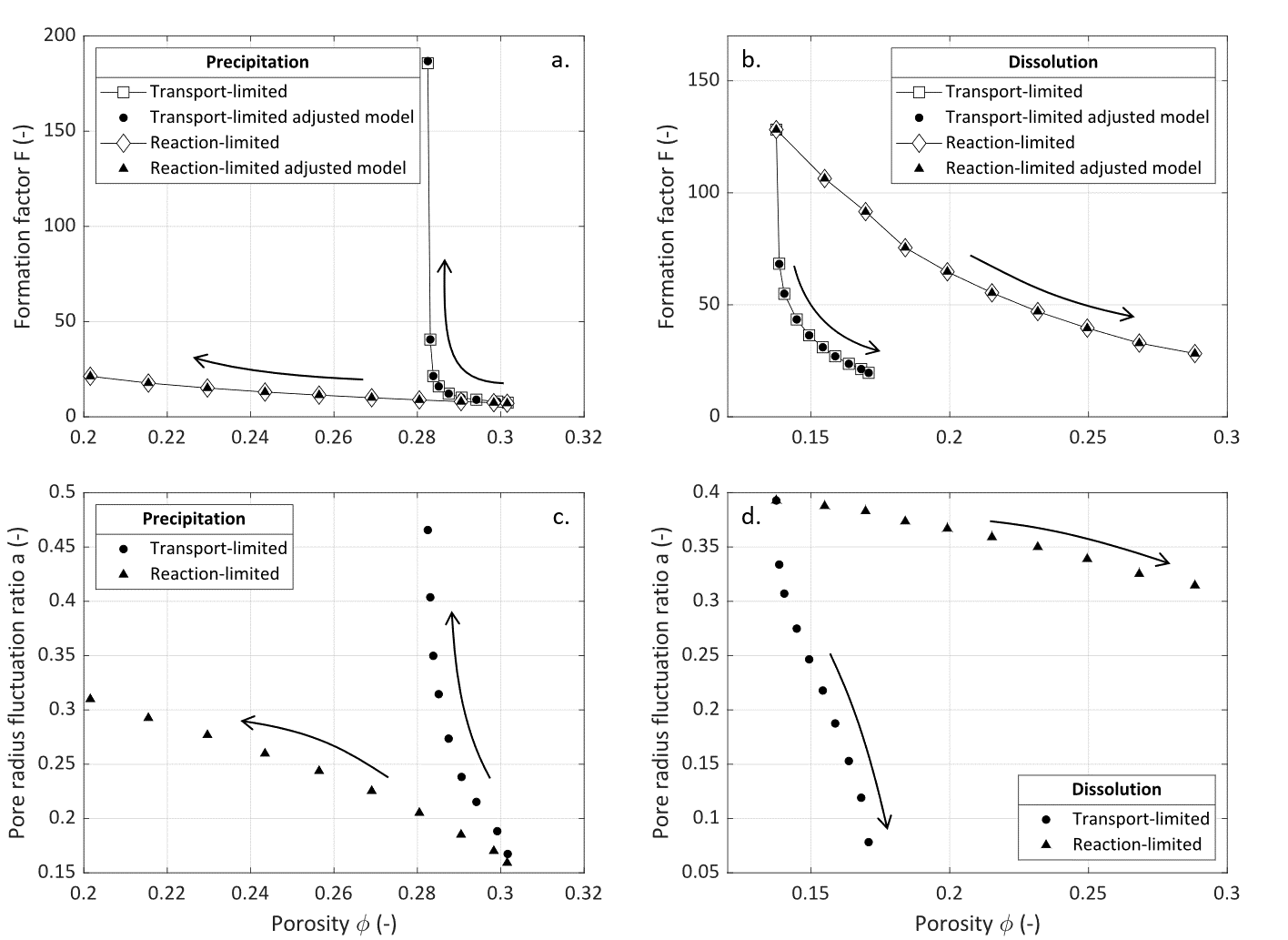
Figure 8: Electrical simulation results for two limiting cases (tansport-limited and reaction-limited) of calcite precipitation and dissolution from Niu and Zhang (2019). Arrows indicate the direction of dissolution or precipitation process evolution. (a) and (b) Formation factor versus porosity obtained by Niu and Zhang (2019) simulations and compared with the adjusted model for precipitation and dissolution, respectively. Model parameters are given in Table 1: the tortuosity $\tau$ is considered to be constant while the pore radius fluctuation ratio $a$ is the only adjustable parameter of the model. (c) and (d) Evolution of the parameter $a$ which increases when the porosity decreases.

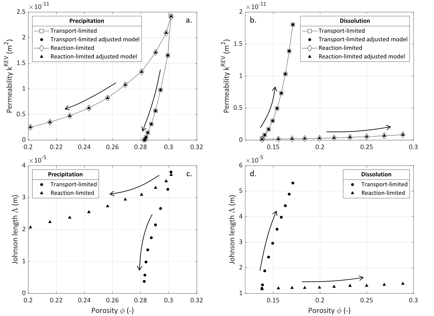
Figure 9: Fluid flow properties simulation results of two limiting cases (tansport-limited and reaction-limited) of calcite precipitation and dissolution from Niu and Zhang (2019). Arrows indicate the direction of dissolution or precipitation process evolution. (a) and (b) Permeability versus porosity obtained by Niu and Zhang (2019) simulations and compared with the proposed model for precipitation and dissolution, respectively. The model parameters are given in Tables 1 and 2: as values of the tortuosity $\tau$ and the pore radius fluctuation ratio $a$ are reused from the formation factor modeling, the Johnson length $\Lambda$ is the only adjustable parameter of the model. (c) and (d) Evolution of the parameter $\Lambda$ which increases with porosity.

The authors of this study justify the shapes of $F$ and $k^{REV}$ curves with their observations on the digital representations of the microstructural evolution. In the reaction-limited case they observe that precipitated or dissolved minerals are uniformly distributed over grain surfaces. This consequently barely affects electrical and fluid flow properties. On the contrary, in the transport-limited case, dissolution and precipitation mainly occur in some specific areas where fluid velocity is high. This significantly modifies electrical and fluid flow patterns. In the case of transport-limited precipitation, new particles accumulate in pore throats while minerals are preferentially dissolved in the already well opened channels.

To adjust the proposed model to the data, a first set of parameters $a$ and $\tau$ has been determined at the initial state with the Monte-Carlo approach. Then, only parameter $a$ is adjusted with the model to each new data point using the least square method. We consider that only $a$ is affected by dissolution and precipitation because these processes mostly affect the pore shape. Indeed, the results of the pore network modeling developed by Steinwinder and Beckingham (2019) to simulate the impact of pore-scale alterations by dissolution and precipitation on permeability, show that pore throats are important parameters to take into account. However, for the proposed model of this study, the assumption that only $a$ varies requires slow processes of dissolution and precipitation in order to keep the cylindrical shape of pores (Guarracino et al., 2014). Besides, we fit parameter $a$ at each time step rather than using the logarithmic law since it lacks physical meaning to explain this parameter time evolution.

Niu and Zhang (2019) computed the hydraulic tortuosity $\tau_{h}$ (-) from the simulated fluid velocity field for all of their data. They found nearly constant values defined between 1 and 2. As we computed $\tau$ = 1.3 and $\tau$ = 1.8 in precipitation and dissolution, respectively, these results are within the predicted range of the simulated data from Niu and Zhang (2019) and confirm our hypothesis that constrictivity is the pore feature most impacted by dissolution and precipitation processes. However, to interpret the evolution of the formation factor during dissolution ($F$ decreases) and precipitation ($F$ increases), Niu and Zhang (2019) computed the electrical tortuosity ($\tau_{e}\leavevmode\nobreak\ =\leavevmode\nobreak\ F\phi$, no unit) of their porous medium and obtained high values (from 2 to 200), varying over 1 to 2 decades for the transport-limited cases. These overestimated values of the medium tortuosity highlight that constrictivity and the bottleneck effect should not be neglected to evaluate how dissolution and precipitation processes affect the pore structure.

Figs. 8a and 8b show that in each case the proposed model accurately fits the data with computed errors lower than 1 % (see Table 1). As presented on Figs. 8c and 8d, parameter $a$ follows monotonous variations: it decreases when the porosity increases. We define $a$ as the ratio of the sinusoidal pore aperture $r^{\prime}$ over the mean pore radius $\mathrm{bar}{r}$ (see the definition of $a$ in section 2.1.1). When $a$ increases, it can be caused by the increase of $r^{\prime}$, which involves a stronger periodical constriction of the pore aperture, and/or by the decrease of the mean pore radius $\mathrm{bar}{r}$. On the contrary, when $a$ decreases, it implies the increase of $\mathrm{bar}{r}$ and/or the decrease of $r^{\prime}$, which lead to thicker pores with smoother pore walls, respectively. These variations are consistent with the fact that precipitation and dissolution affect the pore geometry through the sample. In case of precipitation pore throats shrink while they are enlarged with dissolution. It can also be observed on Figs. 8c and 8d that $a$ shows stronger variations in the transport-limited case than in the reaction-limited case. This is consistent with the fact that transport-limited reactions occur in localized areas which will strongly affect the pore properties.

The relation between the permeability $k^{REV}$ and the Johnson length $\Lambda$ is obtained by combining Eqs. (39) and (42):

$$k^{REV}\leavevmode\nobreak\ =\leavevmode\nobreak\ \Lambda^{2}\leavevmode\nobreak\ \frac{(1-4a^{2})^{3/2}}{1+2a^{2}}\leavevmode\nobreak\ \frac{\phi}{8\tau^{2}}$$ (50)

The values of parameters $a$ and $\tau$ are taken from the adjusted models of the formation factor. Thus, the Johnson length $\Lambda$ is the only adjustable parameter to fit the data and is fitted with the least square method. Values are given in Tables 1 and 2.

Table 2: Values of the Johnson length $\Lambda$ and of the MAPE $\epsilon$ (defined in Eq. (49)) for the modeling of permeability versus porosity for the samples from Niu and Zhang (2019). $\Lambda$ is adjusted with the least square method. Sample names are defined in Table 1.

Sample	$\Lambda$	$\epsilon$
	($10^{-5}$ m)	(%)
Dissolution transport-limited	1.196 - 5.320	0.10
Dissolution reaction-limited	1.167 - 1.380	0.03
Precipitation transport-limited	0.376 - 3.800	0.24
Precipitation reaction-limited	2.069 - 3.711	0.06

On Figs. 9a and 9b, one can observe that for each case the model accurately fits the data with computed errors lower than 1 % (see Table 2). As presented on Figs. 9c and 9d, parameter $\Lambda$ follows monotonous variations: it increases with porosity. It can also be observed that $\Lambda$ varies more in the transport-limited case than in the reaction-limited case. For the reaction-limited dissolution it is even nearly constant. Niu and Zhang (2019) found Johnson lengths with the same order of magnitude and with similar variations except in the case of transport-limited precipitation where their values do not follow a monotonous behavior for low porosity values. Either way, Niu and Zhang (2019) interpret the Jonhson length as an effective radius of their porous medium which shows monotonous variations during precipitation ($\Lambda$ decreases) and dissolution ($\Lambda$ increases). In the proposed model, the parameter $a$ describes how dissolution and precipitation processes affect the shape of the pore radius (i.e., its constrictivity) while $\Lambda$ is linked to the fractal distribution of pore size $D_{p}$ and to the maximum average radius $\mathrm{bar}{r}_{max}$. As we suppose dissolution and precipitation slow enough not to interfere with the pore size distribution, $D_{p}$ remains constant for each sample. On the contrary, when dissolution or precipitations occurs, it is expected for the pores to grow or to shrink, respectively. Therefore, The monotonous variations of $\Lambda$ highlight the increase or decrease of $\mathrm{bar}{r}_{max}$ during dissolution or precipitation, respectively. This result is in accordance with the variations of $a$ which can impact $\mathrm{bar}{r}$. Consequently, we describe the pore space evolution during dissolution and precipitation as illustrated in Fig. 10. Indeed, the decrease of $a$ is caused by dissolution, which enlarges the pore and flattens its pore walls. On the contrary, precipitation affects the pores by increasing $a$, which means that pores shrink and become more periodically constricted because of $r^{\prime}$ increase. We thus believe that this interpretation of the electrical conductivity measurement is an important issue for future research on the impact of dissolution and precipitation on the pore shape.

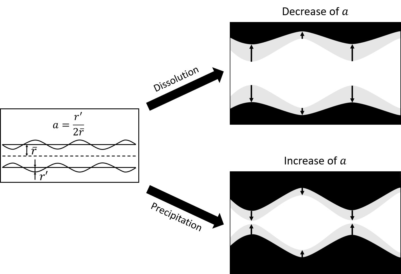
Figure 10: The pore radius fluctuation ratio $a$ is the model parameter which is updated during dissolution and precipitation reactions. Under precipitation $a$ increases, hence the pore aperture varies more. On the contrary $a$ decreases under dissolution and hence the pore becomes smoother.

5 Conclusion

In the present work we express the electrical conductivity and the formation factor of the porous medium in terms of effective petrophysical parameters such as the tortuosity and the constrictivity. The model is based on the conceptualization of the pore space as a fractal cumulative distribution of tortuous capillaries with a sinusoidal variation of their radius (i.e., periodical pore throats). By means of an upscaling procedure, we link the electrical conductivity to transport parameters such as permeability and ionic diffusion coefficient.

The proposed model successfully predicts electrical conductivity and formation factor of unconsolidated samples and natural consolidated rock samples. For datasets of sandstones or carbonates with large range of porosity values, we set that $a$ and $\tau$ follow logarithmic functions of $\phi$. These empirical relations allow the model to accurately fit the datasets. On one hand, for the sandstone samples, the prediction fits much better than previously published models, while on the other hand, the model parameter analysis shows strong agreement with the porosity types description thanks to X-ray microtomography investigations on carbonate samples.

Even if our model is designed for porous media in which the surface conductivity can be neglected, it is possible to take it into account at very low salinity. We do not express it as a function of the pore structure parameters, but determine its value empirically. The comparison of its value with the one found for other models on the same datasets shows that this approach is consistent and reasonable for the purpose of this model.

The model is finally compared to a numerical dataset from simulations of dissolution and precipitation reactions on digital representations of microstructural images. The model can reproduce structural changes linked to these processes by only adjusting a single parameter related to the medium constrictivity: the pore radius fluctuation ratio $a$. We observe that this parameter follows monotonous variations under dissolution or precipitation conditions that makes it a good witness of these chemical processes effect on the pore structure.

We believe that the present study contributes to a better understanding of the links between the electrical conductivity measurement, the pore space characteristics and the evolution of the microstructural properties of the porous medium subjected to dissolution and precipitation processes, therefore enhancing the possibility of using hydrogeophysical tools for the study of carbonate hydrosystems. In the future, we will extend this approach to partially saturated conditions and include these new petrophysical models in an integrated hydrogeophysical approach to better understand hydrosystems in the critical zone.

6 Acknowledgments

The authors warmly thank Qifei Niu and the other anonymous reviewer for the constructive comments that helped to greatly improve the manuscript quality. The authors wish to thank the editor for the effective editing process. The authors strongly thank the financial support of the CNRS INSU EC2CO program for funding the STARTREK (Système péTrophysique de cAractéRisation du Transport Réactif en miliEu Karstique) project. The authors are also very thankful for the wise comments of Roger Guérin.

7 Notations

Parameter	Definition	Unit
$L$	REV length	m
$R$	REV radius	m
$r$	pore radius	m
$\mathrm{bar}{r}$	average pore radius	m
$r^{\prime}$	amplitude of the radius size fluctuation	m
$\lambda$	wavelength	m
$a$	pore radius fluctuation ratio	-
$A_{p}$	REV section area	m2
$l$	tortuous length	m
$\tau$	tortuosity	-
$V_{p}(\mathrm{bar}{r})$	volume of a single pore	m3
$\Sigma_{pore}(\mathrm{bar}{r})$	electrical conductance of a single pore	$S$
$\rho_{w}$	pore water electrical resistivity	$\Omega$.m
$\sigma_{w}$	pore water electrical conductivity	S/m
$\Delta V$	electric voltage	V
$i(\mathrm{bar}{r})$	electric current flowing through a single pore	A
$\sigma_{p}(\mathrm{bar}{r})$	contribution to the porous medium conductivity from a single pore	S/m
$f_{g}$	geometric factor	m
$N(\mathrm{bar}{r})$	number of pores of radius equal or larger than $\mathrm{bar}{r}$	-
$\mathrm{bar}{r}_{max}$	maximum average pore radius	m
$D_{p}$	fractal dimension of pore size	-
$N_{tot}$	total number of pores	-
$\mathrm{bar}{r}_{min}$	minimum average pore radius	m
$\phi$	porosity	-
$I$	REV electric current	A
$\sigma^{REV}$	REV electrical conductivity	S/m
$f$	constrictivity	-
$G$	connectedness	-
$F$	formation factor	-
$Q_{p}(\mathrm{bar}{r})$	flow rate of a single pore	m3/s
$\rho$	density of water	kg/m3
$g$	standard gravity	m/s2
$\mu$	water viscosity	Pa.s
$\Delta h$	hydraulic charge across the REV	m
$Q^{REV}$	total volumetric flow rate	m3/s
$k^{REV}$	REV permeability	m2
$\Lambda$	Johnson length	m
$J_{t}$	diffusive solute mass flow rate	mol/s
$D_{w}$	water diffusion coefficient	m2/s
$D_{eff}$	effective diffusion coefficient	m2/s
$\Delta$c	solute concentration differences	mol/m3
$m$	cementation exponent	-
$\sigma_{s}$	surface conductivity	S/m
$\epsilon$	mean absolute percentage error	%
$N^{d}$	number of data	-
$P^{m}_{i}$	electrical property from the model	-
$P^{d}_{i}$	electrical property from the data	-
$P_{a}$	coefficient to define $a(\phi)$	-
$P_{\tau}$	coefficient to define $\tau(\phi)$	-
$\tau_{h}$	hydraulic tortuosity	-
$\tau_{e}$	electrical tortuosity	-

References

- Archie (1942) G.E. Archie. The electrical resistivity log as an aid in determining some reservoir characteristics. Trans. Am. Inst. Min. Metall. Pet. Eng., 146:54–62, 1942. doi: 10.2118/942054-G.
- Banavar and Johnson (1987) J.R. Banavar and D.L. Johnson. Characteristic pore sizes and transport in porous media. Phys. Rev., 35:7283–7286, 1987. doi: 10.1103/PhysRevB.35.7283.
- Banavar and Schwartz (1987) J.R. Banavar and L.M. Schwartz. Magnetic resonance as a probe of permeability in porous media. Phys. Rev. Lett., 58:1411–1414, 1987. doi: 10.1103/PhysRevLett.58.1411.
- Bernabé and Maineult (2015) Y. Bernabé and A. Maineult. Physics of porous media: fluid flow through porous media. Oxford: Elsevier, in Schubert G., Treatise on geophysics, second ed. edition, 2015. doi: 10.1016/B978-0-444-53802-4.00188-3.
- Binley and Kemna (2005) A. Binley and A. Kemna. DC resistivity and induced polarization methods. Springer, Y. Rubin and S. S. Hubbard (eds.), Hydrogeophysics, 2005. doi: 10.1016/B978-0-444-53802-4.00188-3.
- Binley et al. (2015) A. Binley, S.S. Hubbard, J.A. Huisman, A. Revil, D.A. Robinson, K. Singha, and L.D. Slater. The emergence of hydrogeophysics for improved understanding of subsurface processes over multiple scales. Water Resour. Res., 51:3837–3866, 2015. doi: 10.1002/2015WR017016.
- Bolève et al. (2007) A. Bolève, A. Crespy, A. Revil, F. Janod, and J.L. Mattiuzzo. Streaming potentials of granular media: influence of the dukhin and reynolds numbers. J. Geophys. Res., 112, 2007. doi: 10.1029/2006JB004673.
- Börner and Schön (1991) F.D. Börner and J.H. Schön. A relation between the quadrature component of electrical conductivity and the specific surface area of sedimentary rocks. The log Analist, 32:612–613, 1991. doi: 10.1016/S0301-9322(03)00140-X.
- Broadbent and Hammersley (1957) S.R. Broadbent and J.M. Hammersley. Percolation processes: I. crystals and mazes. Math. Proc. Cambridge Philos. Soc., 53:629–641, 1957. doi: 10.1017/S0305004100032680.
- Bussian (1983) A.E. Bussian. Electrical conductance in a porous medium. Geophysics, 48:1165–1300, 1983. doi: 10.1190/1.1441549.
- Carman (1939) P.C. Carman. Permeability of saturated sands, soils and clays. J. Agric. Sci., 29:263–273, 1939. doi: 10.1017/S0021859600051789.
- Chalikakis et al. (2011) K. Chalikakis, V. Plagnes, R. Guerin, R. Valois, and F.P. Bosch. Contribution of geophysical methods to karst-system exploration: an overview. Hydrogeol. J., 19:1169–1180, 2011. doi: 10.1007/s10040-011-0746-x.
- Chelidze and Gueguen (1999) T.L. Chelidze and Y. Gueguen. Electrical spectroscopy of porous rock: a review - i. theoretical models. Geophys. J. Int., 137:1–15, 1999. doi: 10.1017/S0021859600051789.
- Cherubini et al. (2019) A. Cherubini, B. Garcia, and A. Revil. Influence of CO2 on the electrical conductivity and streaming potential of carbonate rocks. J. Geophys. Res., 124:56–73, 2019. doi: 10.1029/2018JB017057.
- Clennell (1997) B.M. Clennell. Tortuosity: a guide through the maze. Dev. Petrophys. Geol. Soc. Spec. Publ., 122:299–344, 1997. doi: 10.1144/GSL.SP.1997.122.01.18.
- Comiti and Renaud (1989) J. Comiti and M. Renaud. A new model for determining mean structure parameters of fixed beds from pressure drop measurements: Application to beds packed with parallelepipedal particles. Chem. Eng. Sci., 44:1539–1545, 1989. doi: 10.1016/0009-2509(89)80031-4.
- Daily et al. (1992) W. Daily, A. Ramirez, D. Labrecque, and J. Nitao. Electrical resistivity tomography of vadose water movement. Water Resour. Res., 28:1429–1442, 1992. doi: 10.1029/2009JG001129.
- Ellis et al. (2010) M.H. Ellis, M.C. Sinha, Minshull T.A., J. Sothcott, and Best A.I. An anisotropic model for the electrical resistivity of two-phase geologic materials. Geophysics, 75:E161–E170, 2010. doi: 10.1190/1.3483875.
- Fick (1995) A. Fick. On liquid diffusion. J. Memb. Sci., 100:33–38, 1995. doi: 10.1016/0376-7388(94)00230-V.
- Friedman (2005) S.P. Friedman. Soil properties influencing apparent electrical conductivity: a review. Comput. Electron. Agric., 46:45–70, 2005. doi: 10.1016/j.compag.2004.11.001.