Stratified gradient Hamiltonian vector fields and collective integrable systems

Abstract.

We construct completely integrable torus actions on the dual Lie algebra of any compact Lie group $K$ with respect to the standard Lie-Poisson structure. These systems generalize properties of Gelfand-Zeitlin systems for unitary and orthogonal Lie groups: 1) the pullback to any Hamiltonian $K$-manifold is an integrable torus action, 2) if the $K$-manifold is multiplicity free, then the torus action is completely integrable, and 3) the collective moment map has convexity and fiber connectedness properties. They also generalize the relationship between Gelfand-Zeitlin systems and canonical bases via geometric quantization by a real polarization.

To construct these integrable systems, we generalize Harada and Kaveh’s construction of integrable systems by toric degeneration to singular quasi-projective varieties. Under certain conditions, we show that the stratified-gradient Hamiltonian vector field of such a degeneration, which is defined piece-wise, has a flow whose limit exists and defines continuous degeneration map.

1. Introduction

Our work divides in two parts. Part I concerns the construction of completely integrable systems by toric degeneration on Kähler varieties that need not be projective nor smooth. This combines methods from algebraic and symplectic geometry to extend an earlier result of Harada and Kaveh (Sections 3–5 and Appendix A). Our key innovation is the development of a theory of stratified gradient-Hamiltonian vector fields and their flows: we show these flows can be integrated continuously to the limit time 1 despite their singular nature.

Part II applies the results of Part I to construct integrable systems on the dual Lie algebra of any compact connected Lie group. As a consequence, we construct collective integrable systems on Hamiltonian spaces of any compact connected Lie group (Section 6). Our integrable systems have nice topological properties – e.g., convexity, connected fibers, and global action angle coordinates. The moment map images of the resulting collective integrable systems are also closely related to the convex geometry of string polytopes and, via their integer lattice points, crystal bases.

Our motivation is to generalize the construction and properties of Gelfand-Zeitlin integrable systems. Gelfand-Zeitlin integrable systems are intimately related to Gelfand-Zeitlin canonical bases and have applications to geometric quantization, symplectic topology, and non-abelian Duistermaat Heckman measures. The limitation of Gelfand-Zeitlin systems is that they are only known to be completely integrable in the case of unitary and orthogonal groups. Since our collective integrable systems share many properties with Gelfand-Zeitlin systems and have a similar relationship to canonical bases, they can be used to generalize the applications of Gelfand-Zeitlin systems to arbitrary Lie type. We discuss this in more detail at the end of the introduction.

Part I: Stratified Gradient Hamiltonian Vector Fields (Sections 3-5 and Appendix A)

Let $X$ be a complex algebraic variety equipped with a Kähler structure. Harada and Kaveh showed that if $X$ is smooth and projective, and the Kähler structure of $X$ is a constant multiple of a Fubini-Study form, then one can construct completely integrable systems on $X$ by toric degeneration [32]. This result was inspired by Nishinou, Nohara, and Ueda’s construction of Gelfand-Zeitlin completely integrable systems on complex flag manifolds by toric degeneration [44]. Harada and Kaveh’s result is important because completely integrable systems have many applications in symplectic geometry but relatively few examples of completely integrable systems are known. Moreover, completely integrable systems constructed by toric degeneration have nice features which enhance their utility, such as global action-angle coordinates and convex moment map images. Completely integrable systems constructed by toric degeneration can be used to compute lower bounds for the Gromov width of coadjoint orbits [20]. The techniques developed in [32] have also been applied to study symplectic geometry of projective varieties [37] and symplectic cohomological rigidity of symplectic Bott manifolds [46].

The assumptions of the construction in [32] are somewhat unsatisfying from a symplectic geometer’s perspective. First, many symplectic forms on smooth projective varieties are not a constant multiple of a Fubini-Study form. For example, coadjoint orbits of compact Lie groups are smooth projective varieties, but the natural Kostant-Kirillov-Souriau Kähler structure is a constant multiple of a Fubini-Study form if and only if the orbit is parameterized by a constant multiple of a dominant integral weight (with the exception of orbits of rank 1 groups, uncountably infinitely many such orbits do not satisfy this condition). Second, many symplectic manifolds are not projective varieties; for example, some are not compact and some do not admit compatible complex structures. These restrictive assumptions motivate Part I, which extends Harada and Kaveh’s construction to a more general setting where the variety $X$ is not necessarily smooth nor projective. Although constructing integrable systems on non-smooth varieties might initially appear unmotivated from the symplectic perspective, applying this construction to non-smooth affine varieties recovers completely integrable systems on familiar symplectic manifolds – namely coadjoint orbits and, more generally, multiplicity free Hamiltonian K manifolds – in Part II.

We first extend the construction of completely integrable systems by toric degeneration to the case where $X$ is a quasi-projective variety equipped with a decomposition by smooth subvarieties compatible with a Kähler structure. The key ingredient in Harada and Kaveh’s construction is a vector field on the total space of the degeneration, known as the gradient Hamiltonian vector field. In our setting it is no longer possible to define the gradient Hamiltonian vector field on the total space of the toric degeneration because $X$ is singular. Instead, we work with the stratified gradient Hamiltonian vector field of a toric degeneration which we define piecewise. This introduces several technical issues which were not present in [32]. Most notably, the flow on each smooth piece of the degeneration might blow-up, and the flows on the smooth pieces might not fit together continuously. We show that these technical issues can be resolved in the presence of a Hamiltonian torus action, resulting in a construction of completely integrable systems on $X$ by toric degeneration (Theorem 3.7, Corollary 3.9). An illustration of the difference between gradient-Hamiltonian vector fields in the smooth projective setting of Harada-Kaveh and in our non-projective stratified setting is given in Figures 1 and 2.

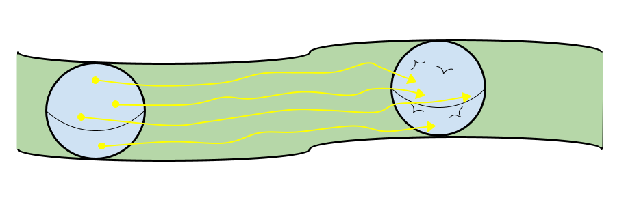
Figure 1. In Harada-Kaveh the time-1 limit of the gradient Hamiltonian flow defines a continuous map from the 1-fiber (left), a smooth projective variety, to the possibly singular toric fiber of the degeneration (right).

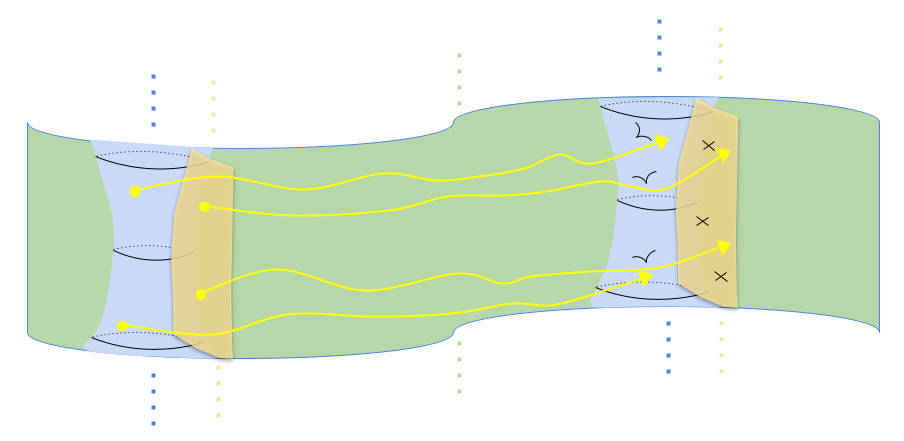
Figure 2. In our work, the 1-fiber (left) is not necessarily smooth nor projective. Instead we suppose it has a decomposition into smooth pieces (illustrated in blue and orange). We define a piecewise gradient Hamiltonian vector field which we call the stratified gradient Hamiltonian vector field. Under some assumptions the time-1 limit of its flow exists and defines a continuous map to the toric fiber (right).

The second part of our generalization of Harada and Kaveh’s construction is concerned with the case where $X$ is a decomposed affine Kähler variety. We provide a general construction of toric degenerations of $X$ that satisfy the assumptions of Theorem 3.7; i.e. we construct toric degenerations where we can integrate the stratified gradient Hamiltonian vector field continuously to the time 1 limit. The ingredients for this construction are a valuation on $X$, a torus action on $X$, and an embedding of $X$ into an inner product space which together satisfy some compatibility conditions (Definition 4.7). We show that the cone generated by the value semigroup of this valuation is the image of the resulting completely integrable system on $X$ (Theorem 4.16).

In Part II, we use an application of these results: we construct completely integrable systems on the affine closure of base affine space, $G\sslash N$, of a complex semisimple Lie group, $G$. The variety $G\sslash N$ is a decomposed affine Kähler variety. We show that completely integrable systems can be constructed by toric degeneration on $G\sslash N$ from the data of a valuation that satisfies certain compatibility conditions (Theorem 5.5). For example, any string valuation gives rise to a completely integrable systems on $G\sslash N$. In this case the moment map image of the resulting completely integrable system is the extended string cone of Berenstein, Zelevinsky, and Littelmann [5, 42], see Example 5.6. The integer lattice points of the extended string cone correspond to elements of a Kashiwara-Lusztig crystal basis for $G$. We note there are many other families of valuations on $G\sslash N$ in the literature that may also produce completely integrable systems this way, provided they satisfy the assumptions of Theorem 5.5 (Example 5.7, Remark 5.8).

Part II: Collective Integrable Systems (Section 6)

The study of collective integrable systems is motivated by a natural question in geometric mechanics: can commuting Hamiltonian symmetries of a symplectic manifold be recovered from non-commuting Hamiltonian symmetries of the same space?

More formally, let $K$ be a compact, connected Lie group and let $M$ be a connected symplectic manifold equipped with a Hamiltonian action of $K$ with equivariant moment map $\mu\colon M\to\operatorname{Lie}(K)^{*}$. Recall that a Hamiltonian function on $M$ is collective with respect to $\mu$ if it can be expressed as the pullback of a Hamiltonian from $\operatorname{Lie}(K)^{*}$ by $\mu$ [27]. A collective (completely) integrable system is a (completely) integrable system consisting of collective Hamiltonians with respect a given moment map. To construct collective integrable systems it is sufficient to construct integrable systems on $\operatorname{Lie}(K)^{*}$ because $\mu$ is a Poisson map with respect to the Lie-Poisson structure on $\operatorname{Lie}(K)^{*}$. Whether a completely integrable system on $\operatorname{Lie}(K)^{*}$ pulls back to a collective completely integrable system on $M$ depends primarily on the complexity of the Hamiltonian $K$-action [29].

Part II of our paper has two main results. First, we construct completely integrable systems on $\operatorname{Lie}(K)^{*}$ for any compact Lie group $K$. The construction is summarized in the following commuting diagram.

(1)

In this diagram $X_{0}$ is the special fiber of a toric degeneration of $G\sslash N$, $\phi$ is the time-1 limit of the stratified gradient-Hamiltonian flow, which exists by the results of Part I, $\Psi$ is the toric moment map of $X_{0}$, and $\mathbb{T}$ is a compact torus of dimension $\frac{1}{2}(\dim_{\mathbb{R}}(K)+\dim_{\mathbb{R}}(Z))$, where $Z$ is the center of $K$.

In (1), the integrable system $\Psi\circ\phi$ descends under a natural quotient $\mu_{R}\colon G\sslash N\to\operatorname{Lie}(K)^{*}$ and induces the continuous map denoted $F$. The coordinates of $F$ define a completely integrable system on each orbit-type stratum of $\operatorname{Lie}(K)^{*}$ (Theorem 6.2). This diagram exists for any valuation on $G\sslash N$ that satisfies the assumptions of Theorem 5.5. For example, every string valuation produces a completely integrable system on $\operatorname{Lie}(K)^{*}$ whose moment map image is the associated extended string cone (Example 6.3).

Second, we show that any collective integrable system constructed from $F$ has nice properties. The following theorem is proved in Section 6.3.

Theorem 1.1.

Let $K$ be a compact connected Lie group, and let $F\colon\operatorname{Lie}(K)^{*}\to\operatorname{Lie}(\mathbb{T})^{*}$ be constructed as in (1).

1. Let $M$ be any connected symplectic manifold equipped with a Hamiltonian action of $K$ with equivariant moment map $\mu\colon M\to\operatorname{Lie}(K)^{*}$. Then the composition

   $$\mu_{\mathbb{T}}\colon M\xrightarrow{\mu}\operatorname{Lie}(K)^{*}\xrightarrow{F}\operatorname{Lie}(\mathbb{T})^{*}$$

   is a moment map for a Hamiltonian action of $\mathbb{T}$ on a connected, open, dense subset $D\subset M$.

2. The complexity of the $\mathbb{T}$ action on $D$ equals the complexity of the $K$ action on $M$. In particular, the action of $K$ on $M$ is multiplicity free (complexity 0) if and only if the action of $\mathbb{T}$ on $D$ is completely integrable (complexity 0).

3. If $M$ is compact, then the fibers of $\mu_{\mathbb{T}}$ are connected and $\mu_{\mathbb{T}}(M)$ is a rational convex polytope that projects linearly onto the Kirwan polytope of $\mu$. In this case, $D$ equals the preimage under $\mu_{\mathbb{T}}$ of the smooth locus of the rational polytope $\mu_{\mathbb{T}}(M)$.

Although this result is non-trivial, its proof follows with relative ease from the results of Part I. In Figure 3, we illustrate how this result applies to different families of Hamiltonian manifolds.

Figure 3. This figure illustrates the relationship between various families of symplectic manifolds and our constructions of integrable systems. The family of Hamiltonian $K$-manifolds is denoted $\mathcal{H}$, the family of compact Hamiltonian $K$-manifolds is denoted $\mathcal{H}_{c}$, and the family of multiplicity free Hamiltonian $K$-manifolds is denoted $\mathcal{M}$. Our construction produces dense torus actions on any manifold in $\mathcal{H}$, Theorem 1.1(A), and completely integrable dense torus actions on any manifold in $\mathcal{M}$, Theorem 1.1(B). When applied to manifolds in $\mathcal{H}_{c}$, our construction produces moment maps with nice topological properties such as connected fibers and images that are rational convex polytopes, Theorem 1.1(C). If $K$ is a unitary or orthogonal group, then collective Gelfand-Zeitlin systems have the same properties [28, 29, 40]. The family of smooth projective varieties is denoted $\mathcal{P}$ and the family of coadjoint orbits of $K$ is denoted $\mathcal{C}$. Harada and Kaveh’s construction applies to manifolds in $\mathcal{P}$ equipped with a toric degeneration [32, Theorem A]. The intersection $\mathcal{P}\cap\mathcal{M}\cap\mathcal{H}_{c}$ contains the special case of Harada-Kaveh applied to spherical $G$ varieties [32, Theorem 3.37].

We note that conclusion (A) of Theorem 1.1 is non-trivial, even assuming the existence of a completely integrable system $F$, because of the nutation effect phenomenon: a collective Hamiltonian function that generates a periodic action on $\operatorname{Lie}(K)^{*}$ need not generate a periodic action on $M$ when it is pulled back by a moment map [28, Section 4]. Our result produces collective integrable systems that are free of nutation effects by construction.

In the case where $M$ is a compact, multiplicity free $K$-manifold, Theorem 1.1 (C) can be used to put a toric chart on the dense subset $D$ via the classification of proper toric symplectic manifolds [35]. This toric chart is the product of a certain dense convex subset of the moment map image $F\circ\mu(M)$ and the torus $\mathbb{T}$, equipped with standard action-angle coordinates. The moment map image $F\circ\mu(M)$ is described in Proposition 6.10.

In the following subsection, we discuss how Theorem 1.1 can be viewed as a generalization of Gelfand-Zeitlin integrable systems.

Generalizing Gelfand-Zeitlin integrable systems

This subsection gives a historical survey of Gelfand-Zeitlin systems, their applications, and attempts to generalize their properties to arbitrary Lie type. Throughout, Figure 3 serves as a visual guide to the various families of manifolds and constructions of (completely integrable) torus actions in the literature.

Gelfand-Zeitlin systems are completely integrable systems on $\operatorname{Lie}(U(n))^{*}$ introduced by Guillemin and Sternberg [28]. After identifying $\operatorname{Lie}(U(n))^{*}$ with the space of Hermitian $n\times n$ matrices in the standard manner, the coordinates of a Gelfand-Zeitlin system can be defined as the ordered eigenvalues of a sequence of nested principal minors of consecutive dimensions. The image of $\operatorname{Lie}(U(n))^{*}$ under any Gelfand-Zeitlin system is the convex polyhedral cone defined by the interlacing inequalities of the eigenvalues, also known as a Gelfand-Zeitlin cone. Gelfand-Zeitlin systems are so-called because the integer lattice points of the Gelfand-Zeitlin cone – i.e., tuples of interlacing integer eigenvalues of consecutive principal minors – correspond to elements of the Gelfand-Zeitlin canonical bases of irreducible unitary representations [24]. A similar construction yields completely integrable systems with the same properties for orthogonal groups.

Gelfand-Zeitlin systems have been used in many applications. In [28], Gelfand-Zeitlin systems were used to demonstrate independence of polarization for the geometric quantization of integral unitary coadjoint orbits: integer lattice points in the moment map image of the Gelfand-Zeitlin system correspond to a basis of both the Bohr-Sommerfeld quantization via the Gelfand-Zeitlin system and the standard complex quantization. They have also been applied to prove tight lower bounds for the Gromov width of unitary and orthogonal coadjoint orbits [45]. More recently, Gelfand-Zeitlin systems have been used by Crooks and Weitsman to prove new independence of polarization results for the cotangent bundle $T^{*}U(n)$ [17], abelianize symplectic quotients [15], and study non-abelian Duistermaat Heckman measures [16]. Gelfand-Zeitlin systems have also been used to identify new examples of Hamiltonian non-displaceable Lagrangian tori in unitary coadjoint orbits [44].

These applications rely on the fact that Gelfand-Zeitlin integrable systems share the same properties as those given in Theorem 1.1: (A) they produce collective torus actions on any Hamiltonian $U(n)$ manifold [28], (B) they produce completely integrable collective torus actions if the Hamiltonian manifold is multiplicity free [29], and (C) their collective moment maps have nice topological properties if the Hamiltonian manifold is compact or proper [40]. Applications to geometric quantization also rely on the relationship between Gelfand-Zeitlin integrable systems and Gelfand-Zeitlin canonical bases. Thus, Theorem 1.1 – and the relationship between our construction and canonical bases – provides a tool to generalize these applications to arbitrary compact Lie groups.

Constructing integrable systems on $\operatorname{Lie}(K)^{*}$ for arbitrary compact $K$ has been an area of research interest since [28]. The original Gelfand-Zeitlin construction can be generalized to all Lie types, however it only produces completely integrable systems on the dual of unitary or orthogonal Lie algebras. As a consequence, the analogue of Theorem 1.1(B) only holds for the original Gelfand-Zeitlin construction when it is applied to unitary or orthogonal Lie groups. There are other constructions of completely integrable systems on $\operatorname{Lie}(K)^{*}$, such as Mischenko-Fomenko systems for general Lie type [43] and Gelfand-Zeitlin-Molev systems for symplectic type in [31]. However, none are known to have properties (A) or (C) of Theorem 1.1, nor well-understood convex polyhedral cones as their moment map images, nor a direct relation between their moment map images and the representation theory of the group $K$. This prevents the applications of Gelfand-Zeitlin systems mentioned above from being generalized to arbitrary Lie type in an obvious way.

Nishinou, Nohara, and Ueda showed that Gelfand-Zeitlin systems on integral unitary coadjoint orbits can be recovered via toric degeneration of the coadjoint orbit to a singular toric variety [44]. Their construction was later generalized by Harada and Kaveh to smooth projective varieties [32]. In particular, when Harada and Kaveh’s construction is applied to smooth projective spherical $G$-varieties, $G=K^{\mathbb{C}}$, whose a Kähler structure arises from a $G$-linearized very ample line bundle, it produces completely integrable, densely defined torus actions which share many of the properties of Gelfand-Zeitlin systems [32, Theorem 3.37]. Their construction produces moment map images whose integer lattice points are related to canonical bases and has been used to extend independence of polarization results [30]. The key difference, however, between Harada-Kaveh in the spherical case and Gelfand-Zeitlin, is that the construction of Harada-Kaveh is not collective: it produces completely integrable systems directly on the symplectic manifold with no obvious relationship to the moment map of the $K$ action. The relationship between the families of symplectic manifolds to which Harada-Kaveh and Gelfand-Zeitlin can be applied is illustrated in Fig. 3.

A different approach to generalizing Gelfand-Zeitlin systems via connections with Poisson-Lie groups was recently explored by Yanpeng Li, Anton Alekseev and the authors. The first result in this direction showed that the Gelfand-Zeitlin systems on $\operatorname{Lie}(U(n))^{*}$ can be recovered as a tropical limit of Ginzburg-Weinstein diffeomorphisms in certain cluster coordinates [3]. Subsequent work succeeded in extending parts of this limit theory to arbitrary Lie type [1, 2], but we were not able to generalize properties (A)–(C) of Gelfand-Zeitlin systems. Although we were able to construct torus actions on an exhaustive sequence of open subsets of Hamiltonian $K$ manifolds, analytical challenges prevented us from constructing a densely defined torus action in the limit. Moreover, our theory only applied to Hamiltonian $K$ manifolds whose moment map image intersects the set of regular elements of $\operatorname{Lie}(K)^{*}$. For example, the results of [3, 1, 2] only apply to regular coadjoint orbits.

Theorem 1.1 is the first generalization of the properties (A) – (C) of unitary and orthogonal Gelfand-Zeitlin systems to arbitrary Lie type. Moreover, when our construction is applied to a string valuation it produces an integrable system on $\operatorname{Lie}(K)^{*}$ whose moment map image is the corresponding extended string cone, the integral lattice points of which correspond to elements of a crystal basis. As a result, our construction should allow applications of Gelfand-Zeitlin systems to be generalized to arbitrary Lie type. The next section discusses several of those applications in more detail.

Applications

We provide two applications of Theorem 1.1 where the moment map image is not difficult to describe: coadjoint orbits (Example 6.13) and cotangent bundles (Example 6.14) of arbitrary compact connected Lie groups. The former is related to the study of Gromov width and the latter to geometric quantization. Finally, we discuss connections with the recent work of Crooks and Weitsman on non-abelian Duistermaat-Heckman measures.

Our first application is to computing the Gromov width of coadjoint orbits of compact Lie groups (see Example 5.6 and Section 6.5). Karshon and Tolman have conjectured a simple formula for the Gromov width of coadjoint orbits of semisimple compact Lie groups and tight upper bounds are known in all cases [11]. Tight lower bounds were proven for all orbits in type A, B, D using Gelfand-Zeitlin systems [45]. Tight lower bounds were later generalized to most coadjoint orbits of arbitrary Lie type using Harada-Kaveh in [20], but a gap in the generalization to arbitrary Lie type remains (see the end of Section 6.5 for additional details). This gap highlights the difference between Gelfand-Zeitlin and Harada-Kaveh: Harada-Kaveh cannot produce integrable systems on coadjoint orbits that are not parameterized by a scalar multiple of a dominant integral weight (aka irrational orbits) because their symplectic forms cannot be written as a constant multiple of a Fubini-Study Kähler form on the orbit. Although one might naïvely expect that Harada-Kaveh systems, or the resulting lower bounds for Gromov width, might somehow be extended by a continuity argument to the irrational coadjoint orbits (the rational orbits are dense, after all), there is no obvious way that this works. In Section 6.5 we show how the integrable systems we construct on arbitrary coadjoint orbits in arbitrary type (Example 5.6) eliminate this technical roadblock. As a result, we reduce the Karshon–Tolman conjecture to a purely algebraic conjecture regarding the existence of good birational orderings with certain algebraic properties (Theorem 6.15).

Our second application is to cotangent bundles and geometric quantization. We show how completely integrable torus actions can be constructed on a dense subset of $T^{*}K$, for any compact Lie group $K$, by applying our construction to the natural multiplicity free $K\times K$ action on $T^{*}K$ (Example 6.14). This illustrates how our construction can be applied to non-compact Hamiltonian manifolds. Conveniently, this is also a case where the moment map image is relatively easy to describe. If a string valuation is used in the construction, then the integer lattice points in the moment map image can be identified with elements of a crystal basis for $G=K^{\mathbb{C}}$. This recovers a graded isomorphism between two geometric quantizations of $T^{*}K$: the standard real polarization by fibers of cotangent projection and the real polarization resulting from our construction. This generalizes the recent independence of polarization result for $T^{*}U(n)$ that was proven using collective Gelfand-Zeitlin systems and their connection to Gelfand-Zeitlin bases [17]. More generally, we note that our construction produces real polarizations of arbitrary non-compact multiplicity free spaces equipped with $K$-invariant prequantum data. In the case where such manifolds have other polarizations, our construction therefore provides a means to prove new independence of polarization results. In other cases our real polarizations may produce the only known geometric quantization (e.g., if there is no compatible complex structure nor any other known real polarizations).

Finally, we highlight the connection of our construction to the recent work of Crooks and Weitsman on abelianization of symplectic quotients and non-abelian Duistermaat-Heckman measures. Crooks and Weitsman introduce the notion of Gelfand-Zeitlin data, an abstract generalization of the collective complete integrability properties of Gelfand-Zeitlin systems [15, Definition 1]. Unitary and orthogonal Gelfand-Zeitlin systems, as well as the completely integrable systems we construct in Theorem 6.2, are examples of Gelfand-Zeitlin data. Crooks and Weitsman show there are canonical isomorphisms between generic symplectic reductions of Hamiltonian manifolds with respect to $K$ and with respect to the densely defined big torus action generated by a Gelfand-Zeitlin datum [15, Main Theorem]. This result allows them to relate the Radon-Nikodym derivatives of the Duistermaat-Heckman measures on $\operatorname{Lie}(K)^{*}$ tand $\operatorname{Lie}(\mathbb{T})^{*}$ [16]. In comparison, the other well-known method to study Duistermaat-Heckman measures of Hamiltonian $K$-manifolds is to consider the projection of the Duistermaat-Heckman measure on $\operatorname{Lie}(K)^{*}$ onto the positive Weyl chamber. Our construction allows these results to be applied to any compact Lie group $K$, not just unitary or orthogonal groups.

Acknowledgements

The authors would like to thank Anton Alekseev, Peter Crooks, Megumi Harada, Yael Karshon, Kiumars Kaveh, Allen Knutson, Chris Manon, Daniele Sepe, and Reyer Sjamaar for helpful suggestions and conversations throughout the course of this project. J.L. would like to thank the Fields Institute and the organizers of the thematic program on Toric Topology and Polyhedral Products for the support of a Fields Postdoctoral Fellowship during writing of this paper.

2. Setup

This section establishes terminology, conventions, and notation and collects several useful lemmas.

2.1. Decomposed spaces and varieties

Following [47, Definition 1.1.1], a decomposed space is a paracompact, Hausdorff, countable topological space $X$ equipped with a locally finite partition by locally closed subspaces (called pieces) such that:

1. Every piece is equipped with the structure of a smooth manifold that is compatible with the subspace topology

2. (Frontier condition) If $X^{\sigma}\cap\overline{X^{\tau}}\neq\emptyset$ for a pair of pieces $X^{\sigma},X^{\tau}$ of $X$, then $X^{\sigma}\subset\overline{X^{\tau}}$.

We often denote the pieces of a decomposed space $X$ by $X^{\sigma}$, where $\sigma$ is an element of an indexing set $\Sigma$. Let $\prec$ denote the partial order by inclusion with respect to closures on the set of pieces of a decomposed space. We also equip the indexing set with this partial order.

By a variety we mean an irreducible quasi-projective variety over the complex numbers. Let $\mathbf{I}(X)\subset\mathbb{C}[\mathbb{C}^{n}]$ denote the ideal of functions vanishing on $X\subset\mathbb{C}^{n}$. Let $\mathbf{V}(I)\subset\mathbb{C}^{n}$ denote the vanishing locus of an ideal $I\subset\mathbb{C}[\mathbb{C}^{n}]$. All algebras we consider will be integral domains. Given an algebra $A$ we make no distinction between the affine scheme $\operatorname{Spec}A$ and its set of closed points. A decomposed variety is a variety $X$, equipped with a partition by finitely many smooth irreducible subvarieties $X^{\sigma}$, which endows $X$ with the structure of a decomposed space with respect to its analytic topology.

Definition 2.1.

A decomposed Kähler variety is a tuple $(X,M,\omega)$ where: (i) $X$ is a decomposed variety, (ii) $M$ is a smooth variety equipped with a Kähler form $\omega$ (compatible with the complex structure on $M$), and (iii) $X$ is equipped with an algebraic embedding into $M$ as a (not necessarily closed) subvariety.

The embedding is implicit in our tuple notation for decomposed Kähler varieties. If $M$ is a vector space and $\omega$ is linear, then we say that $(X,M,\omega)$ is a decomposed affine Kähler variety.

2.2. Convex geometry

A lattice is a free $\mathbb{Z}$-module of finite rank. Given a lattice $L$, denote $L^{\vee}=\operatorname{Hom}(L,\mathbb{Z})$ and $L_{\mathbb{R}}=L\otimes_{\mathbb{Z}}\mathbb{R}$. Given a set $A\subset L$, let $\operatorname{cone}(A)\subset L_{\mathbb{R}}$ denote the cone generated by $A$. We import well-known terminology from [14].

A locally rational polyhedral set is a set $V\subset L_{\mathbb{R}}$ such that for all $p\in V$, there is a neighborhood $U_{p}$ of $p$ in $L_{\mathbb{R}}$ and a rational convex polyhedron $P$ such that $U_{p}\cap V=U_{p}\cap P$. A point $p\in V$ is a smooth point of $V$ if it is a smooth point of this rational convex polyhedron $P$. The smooth locus of $V$ is the set of smooth points of $V$ and the singular locus is its complement.

2.3. Lie theory

Unless stated otherwise, $K$ denotes a compact connected Lie group and $G$ denotes the complex form of $K$. Fix a maximal complex algebraic torus $H\subset G$ and let $T$ be the maximal compact torus $H\cap K$ in $K$. We denote Lie algebras with fraktur letters, e.g. $\operatorname{Lie}(G)=\mathfrak{g}$.

Let $\Lambda\subset\mathfrak{t}^{*}$ denote the lattice of real weights of $T$. We use the convention that each $\lambda\in\Lambda$ corresponds to the character $T\to S^{1}$, $t=\exp(\xi)\mapsto t^{\lambda}=e^{\sqrt{-1}\langle\lambda,\xi\rangle}$, for all $\xi\in\mathfrak{t}$.

Fix a set of positive roots $R_{+}$ and let $\Lambda_{+}\subset\Lambda$ denote the semigroup of dominant real weights. Let $m$ denote the number of positive roots, let $n$ denote the number of simple roots, and let $r=\dim_{\mathbb{R}}T$. Let $\mathfrak{g}_{\alpha}$ denote the $\alpha$-weight subspace of $\mathfrak{g}$. Let $N$ and $N_{-}$ be the opposite unipotent radical subgroups of $G$ with Lie algebras $\mathfrak{n}=\oplus_{\alpha\in R_{+}}\mathfrak{g}_{\alpha}$ and $\mathfrak{n}_{-}=\oplus_{\alpha\in R_{+}}\mathfrak{g}_{-\alpha}$ respectively.

Let $\mathfrak{t}^{*}_{+}\subset\mathfrak{t}^{*}$ denote the positive Weyl chamber that is generated as a rational polyhedral cone by $\Lambda_{+}$. Throughout, $\mathfrak{t}^{*}$ is identified canonically with the subspace $(\mathfrak{k}^{*})^{T}\subset\mathfrak{k}^{*}$ of points fixed by the coadjoint action of $T$. The quotient map for the coadjoint action of $K$, $\mathfrak{k}^{*}\to\mathfrak{k}^{*}/K$, defines a homeomorphism $\mathfrak{t}_{+}^{*}\cong\mathfrak{k}^{*}/K$. The sweeping map is the continuous map $\mathcal{S}\colon\mathfrak{k}^{*}\to\mathfrak{k}^{*}/K\cong\mathfrak{t}_{+}^{*}$.

2.4. Moment maps and singular symplectic spaces

All symplectic manifolds are presumed to be connected. Given a (left) action of $K$ on a smooth manifold $M$ and $\xi\in\mathfrak{k}$, define the fundamental vector field $\xi_{M}\in\mathfrak{X}(M)$ with the sign convention so that $\xi\mapsto\xi_{M}$ is a Lie algebra anti-homomorphism. Our sign convention for the moment map equation of a Hamiltonian $K$ action on a symplectic manifold $(M,\omega)$ is $\omega(\xi_{M},\cdot)=d\langle\mu,\xi\rangle$. All moment maps are equivariant. When working with symplectic representations, we always use the quadratic moment map with $\mu(0)=0$. When working with unitary representations on a finite dimensional complex inner product space $(E,h)$, we always use the linear symplectic form $\omega=-\Im h$. We record the following elementary lemma which will be useful later on.

Lemma 2.2.

Let a compact torus $T$ act by unitary transformations on a finite dimensional complex inner product space $(E,h)$ and let $\mu\colon E\to\operatorname{Lie}(T)^{*}$ be the quadratic moment map with $\mu(0)=0$.

1. Assume that $\mu(E)$ is strongly convex. Given a (closed) face $\overline{\sigma}$ of the polyhedral cone $\mu(E)$, let $T^{\overline{\sigma}}$ denote the connected subtorus with $\operatorname{ann}(T^{\overline{\sigma}})=\mathrm{span}_{\mathbb{R}}(\overline{\sigma})$ and let $\operatorname{Fix}(E,T^{\overline{\sigma}})$ denote the set of fixed points for the action of $T^{\overline{\sigma}}$ on $E$. Then, $\operatorname{Fix}(E,T^{\overline{\sigma}})=\mu^{-1}(\overline{\sigma})$.

2. The quadratic moment map $\mu\colon E\to\operatorname{Lie}(T)^{*}$ is proper if and only if $0$ cannot be written as a non-trivial linear combination (with non-negative coefficients) of the real weights of the representation. Equivalently, $\mu(E)$ is strongly convex.

Proof.

To establish (i): Let $E=\oplus_{\lambda}E_{\lambda}$ be the weight decomposition of $E$ with respect to $T$. If $v\in E$ has weight decomposition $\sum_{\lambda}v_{\lambda}$, $v_{\lambda}\in E_{\lambda}$, then $\mu(v)=\frac{1}{2}\sum_{\lambda}\lambda||v_{\lambda}||^{2}$. It follows from this formula and strong convexity of $\mu(E)$ that $\mu^{-1}(\overline{\sigma})=\oplus_{\lambda\in\overline{\sigma}}E_{\lambda}$. On the other hand, $\operatorname{Fix}(E,T^{\overline{\sigma}})=\oplus_{\lambda\in\operatorname{ann}(T^{\overline{\sigma}})}E_{\lambda}$. The result follows by definition of $T^{\overline{\sigma}}$. The proof of (ii) is a straightforward exercise. ∎

Throughout we will deal with Hamiltonian actions on singular spaces. In this paper, a singular symplectic space is a locally compact, paracompact, Hausdorff, second countable topological space $X$ equipped with a locally finite partition by locally closed subspaces $X^{\sigma}\subset X$ such that each $X^{\sigma}$ is equipped with the structure of a connected symplectic manifold (and the manifold structure is compatible with the subspace topology). For example, every decomposed Kähler variety is a singular symplectic space. Unlike decomposed spaces, our singular symplectic spaces need not satisfy the frontier condition!

We denote the symplectic structure on $X^{\sigma}$ by $\omega^{\sigma}$. The subspaces $X^{\sigma}$ are the symplectic pieces of $X$. A Hamiltonian $K$-space is a pair $(X,\mu)$ where $X$ is singular symplectic space equipped with a continuous action of $K$ and $\mu\colon X\to\mathfrak{k}^{*}$ is a continuous map such that for all $\sigma\in\Sigma$, the action of $K$ preserves $X^{\sigma}$, and $(X^{\sigma},\omega^{\sigma},\mu|_{X^{\sigma}})$ is a Hamiltonian $K$-manifold.

2.5. Affine $G$-varieties

Let $G$ be a reductive algebraic group as above. Given an affine $G$-variety $X$, let $\Lambda(X)\subset\Lambda$ denote the semigroup of highest weights of the $G$-module $\mathbb{C}[X]$ and let $\Gamma(X)=\operatorname{cone}\Lambda(X)$. By [8, Corollary 2.9], the semigroup $\Lambda(X)$ is finitely generated. Let $\Sigma(X)$ denote the set of pieces of $\Gamma(X)$ with respect to its decomposition by relative interiors of closed faces, i.e. each $\sigma\in\Sigma(X)$ is the relative interior of the closed face $\overline{\sigma}\subset\Gamma(X)$. Abbreviate $\Gamma=\Gamma(X)$ and $\Sigma=\Sigma(X)$ when the meaning is clear from context. If $G=H$ is a torus, then let $|f|_{\Lambda}\in\Lambda$ denote the degree of a $\Lambda$-homogeneous element of $\mathbb{C}[X]$. Abbreviate $|f|=|f|_{\Lambda}$ when the torus action is clear from context.

For the rest of this subsection, suppose $G=H$ is a torus. In this case, the decomposition of $\Gamma(X)$ is related to a decomposition of $X$ which will be important in our constructions. Given $\sigma\in\Sigma(X)$, let $T^{\overline{\sigma}}\subset T$ denote the connected subtorus such that $\operatorname{span}_{\mathbb{R}}(\sigma)=\operatorname{ann}(\operatorname{Lie}(T^{\overline{\sigma}}))$ and let $H^{\overline{\sigma}}$ denote the algebraic subtorus of $H$ with maximal compact torus equal to $T^{\overline{\sigma}}$. Let $X^{\overline{\sigma}}$ denote the subvariety $\operatorname{Fix}(X,H^{\overline{\sigma}})$ of points fixed by $H^{\overline{\sigma}}$ and let

(2) $$X^{\sigma}=X^{\overline{\sigma}}\backslash\bigcup_{\tau\prec\sigma}X^{\overline{\tau}}.$$

Assume that $X$ is embedded $H$-equivariantly as a closed subvariety of a finite dimensional $H$-module $E$. If $\Lambda(E)=\Lambda(X)$, then it follows by definition that $X^{\overline{\sigma}}=X\cap E^{\overline{\sigma}}$ as varieties for all $\sigma\in\Sigma(X)=\Sigma(E)$. In fact, slightly more is true.

Lemma 2.3.

With $X$ and $E$ as in the previous paragraph, the scheme-theoretic intersection $X\cap E^{\overline{\sigma}}$ is reduced, i.e. $X^{\overline{\sigma}}=X\cap E^{\overline{\sigma}}$ as schemes.

Proof.

We want to show that ${\bf I}(X)+{\bf I}(E^{\overline{\sigma}})$ is a radical ideal. Let $f\in\mathbb{C}[E]$ such that $f^{k}\in{\bf I}(X)+{\bf I}(E^{\overline{\sigma}})$ for some $k$. We must show that $f\in{\bf I}(X)+{\bf I}(E^{\overline{\sigma}})$. It is a straightforward exercise to show that it suffices to prove the Lemma for $f$ which is homogeneous.

Let us fix a basis $\mathcal{K}=\{z_{1},\dots,z_{J}\}$ of $E^{*}$ consisting of $\Lambda$-homogeneous elements. Note that

(3) $$\mathbf{I}(E^{\overline{\sigma}})=(z_{j}\in\mathcal{K}\mid|z_{j}|\notin\overline{\sigma}).$$

Suppose $f^{k}$ is homogeneous. Then $f^{k}=g+h$, for some homogeneous $g\in{\bf I}(X)$ and $h\in{\bf I}(E^{\overline{\sigma}})$. If $|f^{k}|\in\overline{\sigma}$, then $|h|\in\overline{\sigma}$. The only way this can happen is if $h=0$, so $f^{k}\in{\bf I}(X)$. Since ${\bf I}(X)$ is radical, we have that $f\in{\bf I}(X)\subset{\bf I}(X)+{\bf I}(E^{\overline{\sigma}})$. On the other hand, if $|f^{k}|\notin\overline{\sigma}$ then each monomial term of $f^{k}$ contains some $z_{j}$ with $|z_{j}|\notin\overline{\sigma}$. Then $f^{k}$ vanishes on $E^{\overline{\sigma}}$ so $f^{k}\in{\bf I}(E^{\overline{\sigma}})$. This ideal is also radical, so $f\in{\bf I}(E^{\overline{\sigma}})\subset{\bf I}(X)+{\bf I}(E^{\overline{\sigma}})$. ∎

2.6. Affine toric varieties

We record some notation regarding affine toric varieties. An affine semigroup is a subset of a lattice $L$ that is closed under addition, contains $0$, and is finitely generated. Given an affine semigroup $\mathsf{S}$, let $\mathbb{C}[\mathsf{S}]$ denote the semigroup algebra of $\mathsf{S}$ and let $X_{\mathsf{S}}$ denote the associated affine toric variety.

Let $H$ denote the complex algebraic torus whose lattice of real weights is $L$, and let $T$ be the maximal compact torus in $H$. Let $C\subset L_{\mathbb{R}}$ be a $\operatorname{rank}(L)$-dimensional rational convex polyhedral cone and let $\mathsf{S}=C\cap L$. Then $X_{\mathsf{S}}$ is normal. Let $F\subset C$ be a closed face, let $T^{F}\subset T$ denote the connected subtorus with $\operatorname{span}_{\mathbb{R}}(F)=\operatorname{ann}(\operatorname{Lie}(T^{F}))$, and let $H^{F}$ denote the complex subtorus of $H$ with maximal compact torus equal to $T^{F}$. The subvariety $X^{F}_{\mathsf{S}}=\operatorname{Fix}(X_{\mathsf{S}},H^{F})$ is an $H$ orbit-closure. As a toric variety, $X^{F}_{\mathsf{S}}$ is isomorphic to $X_{\mathsf{S}^{F}}$ where $\mathsf{S}^{F}=\mathsf{S}\cap F$.

3. Stratified gradient Hamiltonian flows

This section concerns a gradient Hamiltonian vector field, placed upon on a degeneration of a decomposed Kähler variety. We describe a set of conditions (GH1)–(GH6) under which this vector field may be integrated to a flow, and under which this flow may be extended continuously across the special fiber of the degeneration. There are two main ways in which our approach extends previous results. First, we do not assume that we work with compact varieties, and so the flow of this vector field may blow up before it reaches the special fiber. Second, because our varieties are decomposed, the gradient Hamiltonian vector field is defined piece-wise, and the associated flow is not continuous a priori. The main result of this section (Theorem 3.7) describes how to overcome both of these difficulties.

We briefly summarize the key ideas and associated notation for Theorem 3.7, which may be used as a road map for reading Section 3.3. We start with a toric degeneration $\mathfrak{X}$ whose 1-fiber, $\mathfrak{X}_{1}$, is a decomposed Kähler variety with pieces denoted by $\mathfrak{X}_{1}^{\sigma}$ for $\sigma$ in an index set $\Sigma$. This degeneration is required to satisfy assumptions (GH1) – (GH6). From this we define a piecewise gradient Hamiltonian vector field on $\mathfrak{X}$. For each $\sigma$ this determines a flow $\varphi_{t}^{\sigma}$ which takes points in $\mathfrak{X}_{1}^{\sigma}$ to points in $\mathfrak{X}_{1-t}^{\sigma}$. These assemble into a continuous function $\varphi_{t}$ from $\mathfrak{X}_{1}$ to $\mathfrak{X}_{1-t}$. Although the time-1 flow $\varphi_{1}$ is not necessarily defined at all points on $\mathfrak{X}_{1}$ because of the singular nature of $\mathfrak{X}_{0}$, the limit as $t\to 1^{-}$ of $\varphi_{t}$ exists for every point in $\mathfrak{X}_{1}$ and defines a continuous map to $\mathfrak{X}_{0}$. The image of each piece $\mathfrak{X}_{1}^{\sigma}$ under this limiting map lies in a toric subvariety $\mathfrak{X}_{0}^{\sigma}\subset\mathfrak{X}_{0}$. The toric subvarieties $\mathfrak{X}_{0}^{\sigma}$ define a partition of $\mathfrak{X}_{0}$ but unlike $\mathfrak{X}_{1}^{\sigma}$ they are not necessarily smooth. Provided that the toric action on $\mathfrak{X}_{0}$ is generated by a moment map, its pullback defines an integrable system on $\mathfrak{X}_{1}$ (see Corollary 3.9).

This construction has an additional feature which is crucial for our applications in Section 6. For each piece $\mathfrak{X}_{1}^{\sigma}$ there is a dense subset $D^{\sigma}\subset\mathfrak{X}_{1}^{\sigma}$ on which the flow $\varphi_{1}^{\sigma}$ is defined and yields a symplectic isomorphism onto the smooth locus $U_{0}^{\sigma}$ of the toric subvariety $\mathfrak{X}_{0}^{\sigma}$ (illustrated in the bottom square of the following diagram).

(4)

Thus, whereas Harada-Kaveh produces a symplectic isomorphism on an open dense subset of their smooth variety, our result produces a symplectic isomorphism on an open dense subset of each piece of our decomposed variety. In particular, the integrable system resulting from pullback defines a toric action on each $D^{\sigma}$ (see Definition 3.10 where we define integrable systems on decomposed Kähler varieties).

This section is organized as follows. Section 3.1 gives basic notions about gradient Hamiltonian vector fields in the stratified setting, and Section 3.2 recalls the definition of a degeneration. The main result of this section, Theorem 3.7, is described in Section 3.3. Its proof is given in Appendix A. Section 3.4 establishes several results about gradient Hamiltonian vector fields on affine varieties which will be used in the sequel.

3.1. Gradient Hamiltonian vector fields

We recall the definition and elementary properties of gradient Hamiltonian vector fields. We refer the reader to [32, Section 2.2] for more details.

Let $M$ be a Kähler manifold and let $\pi\colon M\to\mathbb{C}$ be a holomorphic submersion. Let $\Re\pi,\Im\pi\colon M\to\mathbb{R}$ denote the real and imaginary parts of $\pi$, i.e. $\pi=\Re\pi+\sqrt{-1}\Im\pi$. Let $\nabla(\Re\pi)$ denote the gradient vector field of $\Re\pi$ with respect to the Kähler metric and let $X_{\Im\pi}$ denote the Hamiltonian vector field of $\Im\pi$ with respect to the Kähler form. Since $\pi$ is holomorphic and $M$ is Kähler, it follows that $\nabla(\Re\pi)=-X_{\Im\pi}$. The gradient Hamiltonian vector field of $\pi$ is

(5) $$V_{\pi}:=\frac{X_{\Im\pi}}{||X_{\Im\pi}||^{2}}=-\frac{\nabla\Re\pi}{||\nabla\Re\pi||^{2}}$$

where $||\cdot||$ denotes norm with respect to Kähler metric. The vector field $V_{\pi}$ is defined everywhere on $M$ since $\pi$ is a submersion and therefore $\nabla(\Re\pi)$ is non-vanishing.

Let $M_{z}=\pi^{-1}(z)$ denote the fiber of $\pi$ over $z\in\mathbb{C}$. Let $\varphi_{t}(x)$ denote the flow of $V_{\pi}$ through $x\in M$ at time $t$. If $x\in M_{z}$ and $\varphi_{t}(x)$ is defined, then $\varphi_{t}(x)\in M_{z-t}$. Thus, if $\varphi_{t}(x)$ is defined for all $x\in M_{z}$, then it determines a map $\varphi_{t}\colon M_{z}\to M_{z-t}.$

Since $\pi$ is a holomorphic submersion, each $M_{z}$ is a smooth Kähler submanifold of $M$ and $\dim_{\mathbb{C}}M_{z}=\dim_{\mathbb{C}}M-1$. The following fact is well-known.

Lemma 3.1.

If it is defined, the map $\varphi_{t}\colon M_{z}\to M_{z-t}$ is symplectic with respect to the restricted Kähler forms on $M_{z}$ and $M_{z-t}$.

We now extend the definition of gradient Hamiltonian vector fields to a stratified setting. Let $M$ be a Kähler manifold as before. Let $Y$ be a decomposed space and suppose $Y$ is embedded in $M$ so that each smooth piece $Y^{\sigma}$ is a submanifold. The stratified tangent bundle of $Y$ is the disjoint union of tangent bundles $TY=\bigcup_{\sigma\in\Sigma}TY^{\sigma}.$ It inherits a subspace topology from $TM$. See e.g. [47, Section 2.1] for more details.

Suppose $\pi\colon M\to\mathbb{C}$ is a holomorphic map, each $Y^{\sigma}$ is a Kähler submanifold of $M$, and each restricted map $\pi\colon Y^{\sigma}\to\mathbb{C}$ is a submersion. For each $\sigma\in\Sigma$, let $V_{\pi}^{\sigma}\colon Y^{\sigma}\to TY^{\sigma}$ denote the gradient Hamiltonian vector field of the holomorphic submersion $\pi\colon Y^{\sigma}\to\mathbb{C}$.

Definition 3.2.

The stratified gradient Hamiltonian vector field on $Y$ is the section

(6) $$V_{\pi}\colon Y\to TY,\quad V_{\pi}(x)=V_{\pi}^{\sigma}(x)\text{ for }x\in Y^{\sigma}.$$

Note that $V_{\pi}$ may fail to be continuous. It is a stratified vector field in the sense of [47, 2.1.5].

For $x\in Y$, consider the initial value problem

(7) $$\frac{d}{dt}\varphi_{t}(x)=V_{\pi}(\varphi_{t}(x)),\quad\varphi_{0}(x)=x.$$

A solution of this initial value problem is given by combining the flows of the vector fields $V_{\pi}^{\sigma}$ in a piecewise manner. Let $\varphi_{t}^{\sigma}$ denote the flow of $V_{\pi}^{\sigma}$. Define

(8) $$\varphi_{t}(x)=\varphi_{t}^{\sigma}(x)\quad\text{if $\varphi_{t}^{\sigma}(x)$ is defined}.$$

We call $\varphi_{t}(x)$ the stratified gradient Hamiltonian flow. If $x\in Y\cap M_{z}$ and $\varphi_{t}(x)$ is defined, then $\varphi_{t}(x)\in Y\cap M_{z-t}$.

Because each stratum $Y^{\sigma}$ may be non-compact, it will become necessary to establish in some cases that the flows $\varphi_{t}^{\sigma}$ exist. This becomes possible in the presence of additional group symmetry. The key lemma is a straightforward application of Noether’s theorem. Similar versions of this lemma previously appeared in, e.g. [32, Section 2.6] and [33, Lemma 5.1].

Lemma 3.3.

Let $M$ be a Kähler manifold with Kähler form $\omega$ and Kähler metric $g$, and let $\pi\colon M\to\mathbb{C}$ be a holomorphic submersion. Assume there is a Hamiltonian action of a connected Lie group $K$ on $(M,\omega)$ with moment map $\psi\colon M\to\mathfrak{k}^{*}$ such that the action of $K$ preserves the fibers of $\pi$ and the Kähler metric $g$. Then, as long as it exists, the flow of $V_{\pi}$ is $K$-equivariant and preserves fibers of $\psi$.

3.2. Degenerations

Let $\mathfrak{X}$ be a variety and let $\pi\colon\mathfrak{X}\to\mathbb{C}$ be a morphism. Denote the fiber of $\pi$ over $z\in\mathbb{C}$ by $\mathfrak{X}_{z}$. Let $Z\subset\mathfrak{X}$ denote the union of the singular set of $\mathfrak{X}$ and the critical set of $\pi|_{\mathfrak{X}^{sm}}$, where $\mathfrak{X}^{sm}$ denotes the smooth locus of $\mathfrak{X}$. Then $\mathfrak{X}\setminus Z$ is a complex manifold and $\pi\colon\mathfrak{X}\setminus Z\to\mathbb{C}$ is a holomorphic map. For all $z\in\mathbb{C}$, denote $U_{z}=\mathfrak{X}_{z}\setminus Z$. Since $\pi\colon\mathfrak{X}\setminus Z\to\mathbb{C}$ is a submersion, each $U_{z}$ is a complex submanifold of $\mathfrak{X}\setminus Z$ of complex codimension 1.

We recall the following definition from [32, Definition 2].

Definition 3.4.

A degeneration of a variety $X$ is a map $\pi\colon\mathfrak{X}\to\mathbb{C}$ such that:

1. There is an algebraic isomorphism $\rho\colon X\times\mathbb{C}^{\times}\to\mathfrak{X}\setminus\mathfrak{X}_{0}$ such that $\pi\circ\rho=\operatorname{pr}_{2}$. Such an isomorphism is called a trivialization away from 0.

2. The fiber $\mathfrak{X}_{0}$ is non-empty.

3. $\pi$ is a flat family of varieties, i.e. it is a flat morphism and its fibers are all reduced as schemes.

A degeneration $\pi\colon\mathfrak{X}\to\mathbb{C}$ is a toric degeneration if $\mathfrak{X}_{0}$ is a toric variety.

If $\pi\colon\mathfrak{X}\to\mathbb{C}$ is a degeneration, then $\pi\colon\mathfrak{X}\setminus Z\to\mathbb{C}$ is a submersion onto $\mathbb{C}$. If the variety $X$ is smooth, then it follows by trivialization away from $0$ that $Z$ is contained in $\mathfrak{X}_{0}$. In this case, $U_{z}=\mathfrak{X}_{z}$ for all $z\neq 0$. More generally, we have the following.

Proposition 3.5.

[32, Corollary 2.10] Let $\pi\colon\mathfrak{X}\to\mathbb{C}$ be a degeneration of $X$. Then for all $z\in\mathbb{C}$, $U_{z}$ is precisely the smooth locus of $\mathfrak{X}_{z}$. In particular, $U_{z}$ is dense in $\mathfrak{X}_{z}$.

3.3. Stratified gradient Hamiltonian vector fields

Let $(X,M,\omega)$ be a decomposed Kähler variety (Definition 2.1) and let $\pi\colon\mathfrak{X}\to\mathbb{C}$ be a degeneration of $X$. The trivialization $\rho$ and the decomposition of $X$ allows us to define subfamilies

(9) $$\mathfrak{X}^{\overline{\sigma}}:=\overline{\rho(X^{\sigma}\times\mathbb{C}^{\times})},\quad\mathfrak{X}^{\sigma}:=\mathfrak{X}^{\overline{\sigma}}\setminus\bigcup_{\tau\prec\sigma}\mathfrak{X}^{\overline{\tau}}$$

where closure is with respect to the Zariski topology. The trivialization also yields isomorphisms $\mathfrak{X}^{\overline{\sigma}}\setminus\mathfrak{X}_{0}\cong\overline{X^{\sigma}}\times\mathbb{C}^{\times}$ and $\mathfrak{X}^{\sigma}\setminus\mathfrak{X}_{0}\cong X^{\sigma}\times\mathbb{C}^{\times}$. Denote

(10) $$\mathfrak{X}_{z}^{\overline{\sigma}}:=\mathfrak{X}_{z}\cap\mathfrak{X}^{\overline{\sigma}},\quad\text{and}\quad\mathfrak{X}_{z}^{\sigma}:=\mathfrak{X}_{z}\cap\mathfrak{X}^{\sigma}$$

for all $z\in\mathbb{C}$. Note that $\mathfrak{X}^{\overline{\sigma}}$, $\mathfrak{X}^{\sigma}$, $\mathfrak{X}^{\overline{\sigma}}_{z}$, and $\mathfrak{X}^{\sigma}_{z}$ are subvarieties of $\mathfrak{X}$ for all $\sigma$ and all $z\in\mathbb{C}$.

We now give a list of assumptions (GH1)–(GH6) that we will place on our degenerations. These are partially inspired by Harada and Kaveh’s assumptions (a)–(d) [32, p. 932].

1. For all $\sigma$, the restricted map $\pi\colon\mathfrak{X}^{\overline{\sigma}}\to\mathbb{C}$ is a flat family of varieties.

2. The family $\mathfrak{X}$ is embedded into $M\times\mathbb{C}$ as a subvariety such that the map $\pi\colon\mathfrak{X}\to\mathbb{C}$ coincides with restriction to $\mathfrak{X}$ of the projection $M\times\mathbb{C}\to\mathbb{C}$.

3. The embedding $X=X\times\{1\}\cong_{\rho}\mathfrak{X}_{1}\subset M\times\{1\}=M$ given by assumption (GH2) coincides with the embedding $X\hookrightarrow M$ of the decomposed Kähler variety $(X,M,\omega_{M})$.

For each $\sigma$, define $Z^{\sigma}\subset\mathfrak{X}^{\sigma}$ to be the union of the critical set of $\pi\colon\mathfrak{X}^{\sigma}\to\mathbb{C}$ and the singular set of $\mathfrak{X}^{\sigma}$. Denote $U_{0}^{\sigma}=\mathfrak{X}_{0}^{\sigma}\setminus Z^{\sigma}$. It follows by assumption (GH1) and Proposition 3.5 that $U_{0}^{\sigma}$ is precisely the smooth locus of $\mathfrak{X}_{0}^{\sigma}$, i.e. $U_{0}^{\sigma}=(\mathfrak{X}_{0}^{\sigma})^{sm}$ (see Lemma A.2).

Equip $\mathbb{C}$ with its standard Kähler structure and $M\times\mathbb{C}$ with the product Kähler structure. In particular, the Kähler form is the product symplectic structure $\omega=\omega_{M}\oplus\omega_{\rm{std}}$.

1. There is a Hamiltonian action of a compact torus $T$ on $M\times\mathbb{C}$ with moment map $\psi\colon M\times\mathbb{C}\to\mathfrak{t}^{*}$ such that:

   1. The action of $T$ on $M\times\mathbb{C}$ preserves each of the subvarieties $\mathfrak{X}^{\sigma}\setminus Z^{\sigma}$, the fibers of $\pi$, and the Kähler metric on $M\times\mathbb{C}$.

   2. The map $(\pi,\psi)\colon\mathfrak{X}\to\mathbb{C}\times\mathfrak{t}^{*}$ is proper.

   3. The subfamilies $\mathfrak{X}^{\sigma}$ are saturated by the restricted maps $\psi\colon\mathfrak{X}\to\mathfrak{t}^{*}$.

Note that by assumptions (GH4)II) and (GH4)III), the map $(\pi,\psi)\colon\mathfrak{X}^{\sigma}\to\mathbb{C}\times\mathfrak{t}^{*}$ is proper as a map to its image for every subfamily $\mathfrak{X}^{\sigma}$.

Denote the restriction of $\omega$ to the symplectic submanifolds $\mathfrak{X}^{\sigma}\setminus Z^{\sigma}$, $\mathfrak{X}^{\sigma}_{z}$ for $z\neq 0$, and $U_{0}^{\sigma}$ by $\omega^{\sigma}$, $\omega^{\sigma}_{z}$, and $\omega^{\sigma}_{0}$, respectively. The action of $T$ preserves each of these submanifolds. The restricted action is therefore also Hamiltonian with moment map given by the restriction of $\psi$. The following assumption is sufficient to conclude that the time-1 gradient Hamiltonian flow on $\mathfrak{X}^{\sigma}\setminus Z^{\sigma}$ defines a symplectomorphism from a dense subset of $(\mathfrak{X}^{\sigma}_{1},\omega^{\sigma}_{1})$ onto $(U_{0}^{\sigma},\omega_{0}^{\sigma})$.

1. The Duistermaat-Heckman measures of $(U_{0}^{\sigma},\omega_{0}^{\sigma},\psi)$ and $(\mathfrak{X}^{\sigma}_{1},\omega^{\sigma}_{1},\psi)$ are equal for all $\sigma\in\Sigma$. In particular, $U_{0}^{\sigma}$ is non-empty.

Because $U_{0}^{\sigma}$ is nonempty for all $\sigma\in\Sigma$, each subfamily $\pi\colon\mathfrak{X}^{\overline{\sigma}}\to\mathbb{C}$ is a degeneration.

The partition of $\mathfrak{X}\setminus\mathfrak{X}_{0}$ by the manifolds $\mathfrak{X}^{\sigma}\setminus\mathfrak{X}_{0}^{\sigma}=\rho(X^{\sigma}\times\mathbb{C}^{\times})$ is a decomposition. Each $\mathfrak{X}^{\sigma}\setminus\mathfrak{X}_{0}^{\sigma}$ is a Kähler submanifold of $M\times\mathbb{C}$ and the restricted maps $\pi\colon\mathfrak{X}^{\sigma}\setminus\mathfrak{X}_{0}^{\sigma}\to\mathbb{C}$ are holomorphic submersions. Thus, we may define a stratified gradient Hamiltonian vector field as in Section 3.1,

(11) $$V_{\pi}\colon\mathfrak{X}\setminus\mathfrak{X}_{0}\to T(\mathfrak{X}\setminus\mathfrak{X}_{0}),\quad V_{\pi}(x)=V_{\pi}^{\sigma}(x)\text{ for }x\in\mathfrak{X}^{\sigma}\setminus\mathfrak{X}_{0}^{\sigma}.$$

The following is sufficient to prove that its gradient Hamiltonian flow is continuous.

1. The stratified vector field $V_{\pi}\colon\mathfrak{X}\setminus\mathfrak{X}_{0}\to T(\mathfrak{X}\setminus\mathfrak{X}_{0})$ is continuous.

A first consequence of these axioms is the following. Its proof is an easy application of Lemma 3.3, together with (GH4).

Proposition 3.6.

The flow $\varphi^{\sigma}_{t}\colon\mathfrak{X}^{\sigma}_{1}\to\mathfrak{X}^{\sigma}_{1-t}$ exists, for all $0<t<1$ and all $\sigma\in\Sigma$.

We now state the main result of this section. Its proof is given in Appendix A.

Theorem 3.7.

Let $\pi\colon\mathfrak{X}\to\mathbb{C}$ be a degeneration of a decomposed Kähler variety $(X,M,\omega_{M})$ that satisfies assumptions (GH1)–(GH6) above. Let $T$ and $\psi$ be the compact torus and moment map of assumption (GH4).

Then, for all $x\in\mathfrak{X}_{1}$, the limit

$$\phi(x)=\lim_{t\to 1^{-}}\varphi_{t}(x)$$

exists and defines a continuous, $T$-equivariant, proper, surjective map $\phi\colon\mathfrak{X}_{1}\to\mathfrak{X}_{0}$. Moreover:

1. For all $\sigma\in\Sigma$ and $x\in U_{0}^{\sigma}$, the flow $\varphi_{-1}^{\sigma}(x)$ exists, $D^{\sigma}:=\varphi_{-1}^{\sigma}(U_{0}^{\sigma})$ is a dense open subset of $\mathfrak{X}^{\sigma}_{1}$, and

   $$\phi|_{D^{\sigma}}=\varphi_{1}^{\sigma}\colon(D^{\sigma},\omega_{1}^{\sigma})\to(U_{0}^{\sigma},\omega_{0}^{\sigma})$$

   is a symplectomorphism.

2. $\psi\circ\phi=\psi$.

Remark 3.8.

The construction of the map $\phi$ has two main components: proving that $\varphi_{t}\colon\mathfrak{X}_{1}\to\mathfrak{X}_{1-t}$ is continuous when $t<1$, and proving that the limit $\lim_{t\to 1^{-}}\varphi_{t}(x)$ exists and is continuous. The proof that $\varphi_{t}$ is continuous for $t<1$ relies on assumptions (GH4) and (GH6). There are various other frameworks for studying flows of vector fields on stratified spaces (such as Mather’s control theory or the notion of rugose vector fields), which we did not use in our proof. The proof that the limit $\lim_{t\to 1^{-}}\varphi_{t}(x)$ exists and is continuous follows the same outline as the proof of [32, Theorem 2.12], along with an application of Noether’s theorem (Lemma 3.3).

Our primary application of Theorem 3.7 is to toric degenerations. If the zero fiber of the degeneration $\mathfrak{X}$ carries a Hamiltonian action of a torus $\mathbb{T}$ generated by a moment map $\Psi\colon\mathfrak{X}_{0}\to\operatorname{Lie}(\mathbb{T})^{*}$, then the composition of $\Psi$ with $\phi\colon X=\mathfrak{X}_{1}\to\mathfrak{X}_{0}$ generates a torus action on a dense subset of each piece of $X$ as follows.

Corollary 3.9.

Let $\pi\colon\mathfrak{X}\to\mathbb{C}$ be a toric degeneration of a decomposed Kähler variety $(X,M,\omega_{M})$ that satisfies assumptions (GH1)–(GH6), let $\phi\colon\mathfrak{X}_{1}\to\mathfrak{X}_{0}$ denote the map constructed as in Theorem 3.7, and let $\mathbb{T}$ denote the compact torus of the toric variety $\mathfrak{X}_{0}$. Assume that:

1. The action of $\mathbb{T}$ on $\mathfrak{X}_{0}$ extends to an action on $M\times\{0\}=M$ that is Hamiltonian with moment map $\Psi\colon M\to\operatorname{Lie}(\mathbb{T})^{*}$.

2. The subvarieties $U_{0}^{\sigma}$ are $\mathbb{T}$-invariant.

Then, for each $\sigma\in\Sigma$, the restriction of $\Psi\circ\phi$ to $D^{\sigma}$ is a moment map for a complexity 0 Hamiltonian $\mathbb{T}$-action on $(D^{\sigma},\omega_{1}^{\sigma})$.

In [32, Definition 2.1], Harada and Kaveh give a somewhat non-standard definition of completely integrable systems on singular varieties whose smooth locus is equipped with a symplectic structure. We now give a similar definition that is more suitable to the present setting. First, we define a collection of real valued continuous functions $f_{1},\dots,f_{n}$ on a smooth connected symplectic manifold $M$ to be a completely integrable system if:

1. There exists an open dense subset $D\subset M$ such that the restricted functions $f_{i}|_{D}$ are all smooth and the rank of the Jacobian of $F=(f_{1},\dots,f_{n})$ equals $\frac{1}{2}\dim(M)$ on a dense subset of $D$.

2. The restricted functions $f_{i}|_{D}$ pairwise Poisson commute, i.e. $\{f_{i}|_{D},f_{j}|_{D}\}=0$ for all $1\leq i,j\leq n$.

If the functions $f_{1},\dots,f_{n}$ satisfy condition (i) but not condition (ii), then they form an integrable system. Corollary 3.9 produces a completely integrable system on a decomposed Kähler variety in the following sense.

Definition 3.10.

A collection of real valued continuous functions $f_{1},\dots,f_{n}$ on a decomposed Kähler variety (or, more generally, a singular symplectic space, cf. Section 6) $X$ is a (completely) integrable system if their restriction to each piece of $X$ defines an (completely) integrable system in the sense defined above.

Remark 3.11.

Suppose $X$ is a smooth variety equipped the trivial decomposition, $M$ is a projective space equipped with the Fubini-Study Kähler form, the torus $T$ is trivial, and $\mathfrak{X}$ is a toric degeneration. Then assumptions (GH4)–(GH6) are satisfied automatically. In particular, (GH5) reduces to the statement that the symplectic volumes of $U_{0}$ and $X$ are equal, which follows by flatness of $\mathfrak{X}$ (see the proof of [32, Corollary 2.11]). Thus, Corollary 3.9 reduces to [32, Theorem A].

3.4. Gradient Hamiltonian flows on decomposed affine Kähler varieties

We now turn our attention to gradient Hamiltonian flows on affine varieties. The first main result of this section is Proposition 3.12, which is a useful tool for verifying that (GH6) holds. An application of this result is Theorem 3.14, which says that often the symplectic structure on a decomposed affine Kähler variety is independent of the embedding into an ambient affine space. Throughout this section, $H$ is an algebraic torus with maximal compact torus $T$ and real weight lattice $\Lambda$.

We briefly recall the Whitney A condition from  [47, 1.4.3], which we will need below. Given a $k$-dimensional submanifold $N$ of a smooth manifold $M$ and a sequence of points $\{x_{i}\}_{i\in\mathbb{N}}\subset N$, let $\lim_{i\to\infty}T_{x_{i}}N$ denote the limit of tangent spaces in the Grassmannian of $k$-dimensional subspaces of $TM$. A pair $(N^{\prime},N)$ of submanifolds of $M$ satisfies the Whitney condition (A) if:

1. For any sequence $\{x_{i}\}_{i\in\mathbb{N}}\subset N$ that converges to some $x\in N^{\prime}$, if $\lim_{i\to\infty}T_{x_{i}}N$ exists, then $T_{x}N^{\prime}\subset\lim_{i\to\infty}T_{x_{i}}N$.

A decomposed space satisfies the Whitney condition (A) if each pair of its pieces satisfies the Whitney condition (A).

3.4.1. Continuity of gradient Hamiltonian vector fields

Let $E$ be a finite dimensional $H$-module. Extend the action of $H$ to $E\times\mathbb{C}$ by letting $H$ act trivially on $\mathbb{C}$. Let $\mathfrak{X}$ be a $H$-invariant closed subvariety of $\mathfrak{X}\subset E\times\mathbb{C}$. Import all the notation from Section 2.5. Let $\pi$ denote the projection $E\times\mathbb{C}\to\mathbb{C}$ as well as its restriction to $\mathfrak{X}$. Denote $\mathfrak{X}_{0}=\pi^{-1}(0)\cap\mathfrak{X}$. Assume:

1. The partition of $\mathfrak{X}\backslash\mathfrak{X}_{0}$ into $\mathfrak{X}^{\sigma}\backslash\mathfrak{X}_{0}$, $\sigma\in\Sigma(\mathfrak{X})$, gives $\mathfrak{X}\backslash\mathfrak{X}_{0}$ the structure of a decomposed variety.

2. The decomposition of $\mathfrak{X}\setminus\mathfrak{X}_{0}$ in (D1) satisfies the Whitney condition (A) with respect to the embedding into $E\times\mathbb{C}$.

Suppose $E$ is equipped with a complex inner product $h_{E}$ and the action of $T$ is unitary. Equip $E\times\mathbb{C}$ with the product complex inner product $h_{E}\oplus h_{\mathbb{C}}$ (where $h_{\mathbb{C}}$ is the standard complex inner product). This equips the submanifolds $\mathfrak{X}^{\sigma}\setminus\mathfrak{X}_{0}$, $\sigma\in\Sigma$, with a Kähler structure. Assume that the restricted maps $\pi\colon\mathfrak{X}^{\sigma}\setminus\mathfrak{X}_{0}\to\mathbb{C}$ are submersions for all $\sigma\in\Sigma$. Then, we may define a stratified gradient Hamiltonian vector field $V_{\pi}\colon\mathfrak{X}\backslash\mathfrak{X}_{0}\to T(\mathfrak{X}\backslash\mathfrak{X}_{0})$ as in (6). The goal of this section is to prove the following.

Proposition 3.12.

In the preceding context (everything from the beginning of this subsection, including the assumptions (D1) and (D2)), $V_{\pi}\colon\mathfrak{X}\backslash\mathfrak{X}_{0}\to T(\mathfrak{X}\backslash\mathfrak{X}_{0})$ is continuous.

We first establish a preliminary result. Throughout, identify $E\times\mathbb{C}=T_{x}(E\times\mathbb{C})$ for all $x\in E\times\mathbb{C}$. Limits of tangent spaces are taken within the appropriate Grassmannian.

Lemma 3.13.

Let $\sigma,\tau\in\Sigma(\mathfrak{X})$ with $\sigma\prec\tau$. Let $\{x_{j}\}\subset\mathfrak{X}^{\tau}\setminus\mathfrak{X}_{0}$ be a sequence of points converging to $x\in\mathfrak{X}^{\sigma}\setminus\mathfrak{X}_{0}$. If $\lim_{j\to\infty}T_{x_{j}}\mathfrak{X}^{\tau}$ exists, then $\lim_{j\to\infty}T_{x_{j}}\mathfrak{X}^{\tau}\subset T_{x}\mathfrak{X}^{\sigma}\oplus(E^{\overline{\sigma}}\times\mathbb{C})^{\perp}.$

Proof.

Let $\hat{g}_{1},\dots,\hat{g}_{J}$ be a set of $\Lambda$-homogeneous generators of ${\bm{I}}(\mathfrak{X})$. The tangent space of $\mathfrak{X}$ at $x$ is

$$T_{x}\mathfrak{X}=\{v\in E\times\mathbb{C}\mid(d\hat{g}_{j})_{x}(v)=0\text{ for all }j\in[1,J]\}.$$

Since $\lim_{j\to\infty}T_{x_{j}}\mathfrak{X}^{\tau}\subset T_{x}\mathfrak{X},$ it suffices to show $T_{x}\mathfrak{X}\subset T_{x}\mathfrak{X}^{\sigma}\oplus(E^{\overline{\sigma}}\oplus\mathbb{C})^{\perp}$.

By Lemma 2.3 (and since $\mathfrak{X}^{\sigma}\setminus\mathfrak{X}_{0}$ is an open subset of $\mathfrak{X}^{\overline{\sigma}}\setminus\mathfrak{X}_{0}$),

$$T_{x}\mathfrak{X}^{\sigma}=T_{x}\mathfrak{X}^{\overline{\sigma}}=T_{x}\mathfrak{X}\cap(E^{\overline{\sigma}}\times\mathbb{C}).$$

It follows by (3) that if $|\hat{g}_{j}|\notin\overline{\sigma}$, then $\hat{g}_{j}$ vanishes on $E^{\overline{\sigma}}\times\mathbb{C}$. Thus,

$$T_{x}\mathfrak{X}\cap(E^{\overline{\sigma}}\times\mathbb{C})= \{v\in E\times\mathbb{C}\mid(d\hat{g}_{j})_{x}(v)=0,\text{ for all }j\in[1,J]\text{ such that }|\hat{g}_{j}|\in\overline{\sigma}\}\cap(E^{\overline{\sigma}}\times\mathbb{C}).$$

Combining these equalities, we arrive at

$$T_{x}\mathfrak{X}^{\sigma}=\{v\in E\times\mathbb{C}\mid(d\hat{g}_{j})_{x}(v)=0,\text{ for all }j\in[1,J]\text{ such that }|\hat{g}_{j}|\in\overline{\sigma}\}\cap(E^{\overline{\sigma}}\times\mathbb{C}).$$

Finally, let $v\in T_{x}\mathfrak{X}$ and write $v=v^{\prime}+v^{\prime\prime}$, where $v^{\prime}\in E^{\overline{\sigma}}\times\mathbb{C}$ and $v^{\prime\prime}\in(E^{\overline{\sigma}}\times\mathbb{C})^{\perp}$. If $|\hat{g}_{j}|\in\overline{\sigma}$, then $\hat{g}_{j}$ vanishes on $(E^{\overline{\sigma}}\times\mathbb{C})^{\perp}$ and so $(d\hat{g}_{j})_{x}(v^{\prime\prime})=0$. It follows from the description of $T_{x}\mathfrak{X}$ and $T_{x}\mathfrak{X}^{\sigma}$ above that $v^{\prime}=v-v^{\prime\prime}\in T_{x}\mathfrak{X}^{\sigma}$. Thus, $v\in T_{x}\mathfrak{X}^{\sigma}\oplus(E^{\overline{\sigma}}\times\mathbb{C})^{\perp}$. ∎

Proof of Proposition 3.12.

The gradient of $\Re\pi|_{\mathfrak{X}^{\sigma}\backslash\mathfrak{X}_{0}}$ is computed with respect to the metric on $\mathfrak{X}^{\sigma}\backslash\mathfrak{X}_{0}$ which is the restriction of the fixed Kähler metric on $E\times\mathbb{C}$. Let $x\in\mathfrak{X}^{\sigma}\setminus\mathfrak{X}_{0}$ and take a sequence $\{x_{j}\}_{j\in\mathbb{N}}\in\mathfrak{X}\backslash\mathfrak{X}_{0}$ converging to $x$. By passing to a subsequence, we may assume that $\{x_{j}\}_{j\in\mathbb{N}}\subset\mathfrak{X}^{\tau}\setminus\mathfrak{X}_{0}$ for some $\tau\in\Sigma(\mathfrak{X})$ with $\sigma\prec\tau$, and that $\lim_{j\to\infty}T_{x_{j}}\mathfrak{X}^{\tau}$ exists. By Definitions (5) and (6) and Lemma A.5, it suffices to show that $\lim_{j\to\infty}\nabla_{x_{j}}(\Re\pi|_{\mathfrak{X}^{\tau}})=\nabla_{x}(\Re\pi|_{\mathfrak{X}^{\sigma}}).$

In what follows, if $W$ is a linear subspace of $E\times\mathbb{C}$, then $\operatorname{pr}_{W}$ denotes orthogonal projection to $W$. We have

$$\lim_{j\to\infty}\nabla_{x_{j}}(\Re\pi|_{\mathfrak{X}^{\tau}}) =\lim_{j\to\infty}\operatorname{pr}_{T_{x_{j}}\mathfrak{X}^{\tau}}\left(-\frac{\partial}{\partial t}\right)$$

$$=\operatorname{pr}_{\lim_{j\to\infty}T_{x_{j}}\mathfrak{X}^{\tau}}\left(-\frac{\partial}{\partial t}\right)$$

$$=\operatorname{pr}_{\lim_{j\to\infty}T_{x_{j}}\mathfrak{X}^{\tau}}\circ\operatorname{pr}_{T_{x}\mathfrak{X}^{\sigma}\oplus(E^{\overline{\sigma}}\times\mathbb{C})^{\perp}}\left(-\frac{\partial}{\partial t}\right)$$

$$\qquad\qquad\left(\text{by Lemma \ref{lemma;decomplemma}}\right)$$

$$=\operatorname{pr}_{\lim_{j\to\infty}T_{x_{j}}\mathfrak{X}^{\tau}}\left(\operatorname{pr}_{T_{x}\mathfrak{X}^{\sigma}}\left(-\frac{\partial}{\partial t}\right)+\operatorname{pr}_{(E^{\overline{\sigma}}\times\mathbb{C})^{\perp}}\left(-\frac{\partial}{\partial t}\right)\right)$$

$$=\operatorname{pr}_{\lim_{j\to\infty}T_{x_{j}}\mathfrak{X}^{\tau}}\left(\operatorname{pr}_{T_{x}\mathfrak{X}^{\sigma}}\left(-\frac{\partial}{\partial t}\right)\right)$$

$$=\operatorname{pr}_{T_{x}\mathfrak{X}^{\sigma}}\left(-\frac{\partial}{\partial t}\right)$$

$$\qquad\qquad\left(\text{by assumption \ref{D2}}\right)$$

$$=\nabla_{x}(\Re\pi|_{\mathfrak{X}^{\sigma}}).$$

This proves the claim. ∎

3.4.2. Isomorphisms between decomposed affine Kähler varieties

Let $X$ be an affine $H$-variety and import the notation from Section 2.5. Suppose that $X$ embeds as a $H$-invariant closed subvariety of a $H$-module $E$. We introduce the following conditions, which are analogues of (D1) and (D2) for $X$:

1. The partition of $X$ into $X^{\sigma}$, $\sigma\in\Sigma(X)$, gives $X$ the structure of a decomposed variety.

2. The decomposition of $X$ in (D1’) satisfies the Whitney condition (A) with respect to the embedding into $E$.

We now give the first application of Proposition 3.12. Let $(E,h_{E})$ and $(E^{\prime},h_{E^{\prime}})$ be two unitary $T$-modules, with symplectic forms $\omega_{E},\omega_{E^{\prime}}$ and $T$-equivariant moment maps $\mu,\mu^{\prime}$, respectively. Let $i\colon X\hookrightarrow E$ and $i^{\prime}\colon X\hookrightarrow E^{\prime}$ be two closed $H$-equivariant embeddings. We assume without loss of generality that $X$ is not contained in any proper affine subspace of $E$ or $E^{\prime}$. That is, we assume that no $f\in E^{*}\backslash\{0\}$ restricts to a constant function on $X$. In particular, because $X$ is irreducible $\Lambda(E)=\Lambda(X)=\Lambda(E^{\prime})$ (see also Remark 4.9). The embeddings $i$ and $i^{\prime}$ each endow $X$ with the structure of a Hamiltonian $T$-space. Denote these Hamiltonian $T$-spaces $(X_{E},\mu)$ and $(X_{E^{\prime}},\mu^{\prime})$ respectively.

Theorem 3.14.

Assume $X$ satisfies (D1’) and the embeddings $i,i^{\prime}$ both satisfy (D2’). If the moment maps $\mu\colon E\to\mathfrak{t}^{*}$ and $\mu^{\prime}\colon E^{\prime}\to\mathfrak{t}^{*}$ are proper, then $(X_{E},\mu)$ is isomorphic to $(X_{E^{\prime}},\mu^{\prime})$ as a Hamiltonian $T$-space.

Proof.

Consider the unitary $T$-module $(E\times E^{\prime}\times\mathbb{C},h=h_{E}\oplus h_{E^{\prime}}\oplus h_{\mathbb{C}})$ with symplectic structure $\omega=-\operatorname{Im}h$. The action of $T$ is Hamiltonian with moment map $\psi=\mu\circ\operatorname{pr}_{E}+\mu^{\prime}\circ\operatorname{pr}_{E^{\prime}}$. Consider the trivial degeneration $\mathfrak{X}=X\times\mathbb{C}$ of $X$. Embed $\mathfrak{X}$ into $E\times E^{\prime}\times\mathbb{C}$ according to the map

$$X\times\mathbb{C} \to E\times E^{\prime}\times\mathbb{C}$$

$$(x,t) \mapsto(ti(x),(1-t)i^{\prime}(x),t).$$

Its image is a closed $H$-invariant subvariety of $E\times E^{\prime}\times\mathbb{C}$. It has smooth pieces $\mathfrak{X}^{\sigma}=X^{\sigma}\times\mathbb{C}=(X\times\mathbb{C})\cap(E^{\sigma}\times{E^{\prime}}^{\sigma}\times\mathbb{C})$.

We apply Theorem 3.7 to the degeneration $X\times\mathbb{C}\to\mathbb{C}$. To do so, we need to check the conditions (GH1)–(GH6). The conditions (GH1), (GH2), and (GH3), and (GH4)I) are satisfied automatically.

To show (GH4)II), it suffices to show that $(\psi,\pi)\colon E\times E^{\prime}\times\mathbb{C}\to\mathfrak{t}^{*}\times\mathbb{C}$ is proper. By Lemma 2.2(ii), because $\mu$ and $\mu^{\prime}$ are assumed to be proper, the cone $\Gamma(E)=\Gamma(E^{\prime})$ is strongly convex. It follows that the map $\mu\circ\operatorname{pr}_{E}+\mu^{\prime}\circ\operatorname{pr}_{E^{\prime}}\colon E\times E^{\prime}\to\mathfrak{t}^{*}$ is proper. Thus $(\psi,\pi)\colon E\times E^{\prime}\times\mathbb{C}\to\mathfrak{t}^{*}\times\mathbb{C}$ is proper. The condition (GH4)III) holds because

$$\mathfrak{X}^{\overline{\sigma}}=\mathfrak{X}\cap(E^{\overline{\sigma}}\times{E^{\prime}}^{\overline{\sigma}}\times\mathbb{C})=\mathfrak{X}\cap\psi^{-1}(\overline{\sigma}).$$

Here the last equality is a consequence of Lemma 2.2(i).

In contrast with the general setup of Theorem 3.7, there are no singular points of $X^{\sigma}\times\mathbb{C}$. As a result, the stratified gradient Hamiltonian flow $\varphi_{t}$ is defined for all $t\in\mathbb{R}$, for all points of $X\times\mathbb{C}$. The condition (GH5) is then satisfied automatically.

Finally, it remains to verify condition (GH6). To do this, we apply Proposition 3.12. To apply Proposition 3.12, we need to check that (D1) and (D2) hold for $\mathfrak{X}\subset E\times E^{\prime}\times\mathbb{C}$. This is a straightforward consequence of the fact that, by assumption, the partition of $X$ into $X^{\sigma}$ satisfies (D1’), and that each embedding $X\hookrightarrow E$ and $X\hookrightarrow E^{\prime}$ satisfies (D2’).

After applying Theorem 3.7, we have a $T$-equivariant continuous map $\phi\colon X_{E}\to X_{E^{\prime}}$ which, for each $\sigma\in\Sigma$, restricts to a symplectomorphism $\varphi_{1}^{\sigma}\colon D^{\sigma}\to U_{0}^{\sigma}$ from an open dense subset $D^{\sigma}$ of $X_{E}^{\sigma}$ to an open dense subset $U_{0}^{\sigma}$ of $X_{E^{\prime}}^{\sigma}$. Since $X_{E^{\prime}}^{\sigma}$ is smooth, $D^{\sigma}=X_{E}^{\sigma}$ and $U_{0}^{\sigma}=X_{E^{\prime}}^{\sigma}$. In other words, $\varphi_{1}^{\sigma}$ defines a symplectomorphism of $X_{E}^{\sigma}$ and $X_{E^{\prime}}^{\sigma}$. What is more, $\psi\circ\phi=\psi$. Thus, we have a map of Hamiltonian $T$-spaces $\phi\colon(X_{E},\mu)\to(X_{E^{\prime}},\mu^{\prime})$. The map $\varphi_{-1}$ is an inverse to $\phi$, so $\phi$ is an isomorphism of Hamiltonian $T$-spaces. ∎

4. From valuations to stratified gradient Hamiltonian flows

This section provides a general recipe for constructing integrable systems on a decomposed affine Kähler variety $X$. This is achieved by constructing toric degenerations of $X$ that satisfy all the assumptions of the framework set out in Section 3.3. The construction of toric degenerations given here is similar to [32, Section 3.2, 3.3] which deals with the case where $X$ is a smooth projective variety. Our construction is slightly more detailed, due to the singular nature of $X$. Moreover, many details of the construction cited above do not carry over directly because of differences between the affine and projective settings.

The main ingredients of our toric degeneration construction are a torus action on $X$ and a valuation on the coordinate ring of $X$. These ingredients must satisfy some compatibility conditions which we package in our definition of a good valuation (Definition 4.7). The heart of this section is devoted to showing that suitable toric degenerations can be constructed from good valuations. In particular, we show that toric degenerations constructed from good valuations can be embedded into affine space such that the Kähler structure, the decomposition of $X$, the torus action on $X$, and the big torus action on the toric fiber are all compatible with one another (cf. Propositions 4.11, 4.12, and 4.13). This is achieved using properties of Khovanskii bases and our symplectic isotopy theorem for decomposed affine Kähler varieties (Theorem 3.14).

The general idea of this section is as follows. We start with a torus $T_{\mathsf{c}}$, which we call the control torus, together with an action of $T_{\mathsf{c}}$ on an affine variety $X$. The variety $X$ must be $T_{\mathsf{c}}$-equivariantly embedded in a finite dimensional $T_{\mathsf{c}}$-representation, and this embedding must be such that the partition defined in (2) makes $X$ a decomposed affine Kähler variety. The pieces $X^{\sigma}$ of this decomposition are indexed by the relative interiors $\sigma$ of faces of the weight cone for the action of $T_{c}$. Next, we assume the variety $X$ comes with a valuation $\mathbf{v}$ with values in the weight lattice of a bigger torus $\mathbb{T}$. We require the grading of $\mathbb{C}[X]$ by $T_{\mathsf{c}}$-weights to factor as $\mathsf{c}\circ\mathbf{v}$, where $\mathsf{c}\colon\operatorname{Lie}(\mathbb{T})^{*}\to\mathfrak{t}^{*}_{\mathsf{c}}$ is dual to an embedding of $T_{\mathsf{c}}$ in $\mathbb{T}$. Using the valuation, we realize $X$ as the 1-fiber of a degeneration to the affine toric variety $X_{\mathsf{S}}$ associated with the value semigroup $\mathsf{S}$ of $\mathbf{v}$. By applying the results from the previous section, we arrive at commuting diagrams

(12)

where the right diagram is defined for all $\sigma$. In these diagrams $\psi_{\mathsf{c}}$ is the quadratic moment map for the $T_{c}$ action on $X$ and $\Psi$ is the quadratic moment map for the $\mathbb{T}$ action on $X_{\mathsf{S}}$. The toric variety $X_{\mathsf{S}}$ is partitioned by toric subvarieties $X_{\mathsf{S}}^{\sigma}$ that satisfy $X_{\mathsf{S}}^{\sigma}=\Psi^{-1}(\mathsf{c}^{-1}(\sigma))$. For each face $\sigma$ there is a limiting gradient Hamiltonian flow map $\phi^{\sigma}\colon X^{\sigma}\to X_{\mathsf{S}}^{\sigma}$ that restricts to a symplectomorphism from a dense subset of $X^{\sigma}$ onto the smooth locus of $X_{\mathsf{S}}^{\sigma}$. The maps $\phi^{\sigma}$ assemble into the continuous map $\phi$ in the left diagram which is the time-1 limit of the stratified gradient Hamiltonian flow. The composition $\Psi\circ\phi$ defines a completely integrable system on $X$ in the sense of Definition 3.10.

The section is organized as follows. Section 4.1 provides relevant properties of valuations, Khovanskii bases, and the Rees algebra construction of toric degenerations. Section 4.2 contains our definition of good valuations along with Propositions 4.11 and 4.12. Section 4.3 combines results from the previous sections to produce a toric degeneration with an embedding into affine space that has all the desired properties (Proposition 4.13). We also pause in Section 4.3.2 to collect some facts about the resulting toric moment maps which will be useful later, in Section 6. Finally, everything is combined to produce Theorem 4.16, which is the main result.

4.1. Toric degenerations from valuations

Although the Rees algebra construction for affine varieties is well-known, we will require (in Sections 4.2 and 4.3) that the resulting toric degeneration has several additional properties, the combination of which is possibly less well-known. In particular, we will consider Rees algebras constructed from valuations and the resulting degenerations will be embedded into affine space using a Khovanskii basis. Moreover, the toric degeneration and the embedding into affine space will also need to be compatible with a given torus action on $X$. We provide a package of assumptions for valuations on the coordinate ring of $X$, labelled (v1)–(v5), which are sufficient for the resulting toric degeneration to have the desired properties. In relation to the fact that we will deal with decomposed varieties, we give a careful algebraic description of certain subvarieties of $X$ and associated subfamilies of the toric degeneration in Proposition 4.6.

4.1.1. Valuations

Definition 4.1.

Let $L$ be a lattice equipped with a total order $>$ which respects addition. Let $A$ be an algebra over $\mathbb{C}$. A function $\mathbf{v}\colon A\setminus\{0\}\to L$ is a valuation if, for all nonzero $f,g\in A$, it satisfies the following:

1. $\mathbf{v}(f+g)\leq\max\{\mathbf{v}(f),\mathbf{v}(g)\}$;

2. $\mathbf{v}(cf)=\mathbf{v}(f)$ for all nonzero $c\in\mathbb{C}$;

3. $\mathbf{v}(f+g)=\mathbf{v}(f)+\mathbf{v}(g)$.

Let $L$ and $A$ be as in Definition 4.1, and $\mathbf{v}\colon A\setminus\{0\}\to L$ be a valuation on $A$. Denote the value semigroup $\mathsf{S}_{\mathbf{v}}$, or $\mathsf{S}$ when $\mathbf{v}$ is clear from context. Throughout Section 4, assume that $\mathsf{S}_{\mathbf{v}}$ generates $L$ as a $\mathbb{Z}$-module. In particular, we only consider valuations such that $\mathsf{S}_{\mathbf{v}}\subset L$ is saturated. For $s\in\mathsf{S}$, denote

$$A_{\leq s} =\{f\in A\mid\mathbf{v}(f)\leq s\text{ or }f=0\},\quad A_{<s}=A_{\leq s}\setminus\mathbf{v}^{-1}(s).$$

Recall that $\mathbf{v}$ has one-dimensional leaves if $A_{\leq s}/A_{<s}$ is at most one-dimensional for all $s\in\mathsf{S}$. Let $\operatorname{gr}A$ denote the associated graded algebra. If $A$ is an integral domain and $\mathbf{v}$ has one-dimensional leaves, then $\operatorname{gr}A$ is isomorphic to the semigroup algebra $\mathbb{C}[\mathsf{S}]$ [25, Remark 4.13].

Assume that $\mathbf{v}$ has one-dimensional leaves. A Khovanskii basis for $A$ is a set $\mathcal{K}\subset A\backslash\{0\}$ such that $\mathbf{v}(\mathcal{K})$ generates $\mathsf{S}_{\mathbf{v}}$ [38]. Assume that $\mathcal{K}$ is finite and there exists a lattice $\Lambda$ and a surjective linear map $\mathsf{w}\colon L\to\Lambda$ such that:

1. The total order $>$ on $L$ descends under $\mathsf{w}$ to a total order on $\Lambda$.

2. The image $\mathsf{w}(\mathsf{S}_{\mathbf{v}})$ contains a minimal element with respect to this order.

3. The fibers $\mathsf{w}^{-1}(\lambda)\cap\mathsf{S}_{\mathbf{v}}$ are all finite.

With these assumptions in place, we have the following proposition which is a straightforward generalization of [32, Proposition 3.12]. The “subduction algorithm” proof given there adapts easily to this setting.

Proposition 4.2.

If assumptions (v1)-(v3) hold, then $\mathcal{K}$ generates $A$ as an algebra.

In particular, this situation produces an embedding $X\hookrightarrow E$, where $E$ is dual to the subspace $\operatorname{span}_{\mathbb{C}}\mathcal{K}\subset A$. Assumptions (v1)-(v3) also have the following consequence which will be useful later on. Its proof is a straightforward exercise.

Lemma 4.3.

If assumptions (v1)-(v3) hold, then $\operatorname{cone}(\mathsf{S}_{\mathbf{v}})$ and $\operatorname{cone}(\mathsf{w}(\mathsf{S}_{\mathbf{v}}))$ are strongly convex.

4.1.2. The Rees algebra construction

Let $H$ be an algebraic torus with (real) weight lattice $\Lambda$ and let $X$ be an affine $H$-variety with coordinate algebra $A$. As in the previous section, equip $A$ with a valuation $\mathbf{v}$ with values in $(L,>)$. Assume that $\mathbf{v}$ has one-dimensional leaves and $\mathsf{S}_{\mathbf{v}}$ is finitely generated. Assume there exists a linear map $\mathsf{w}\colon L\to\Lambda$ that satisfies (v1)-(v3) and the following.

1. If $f\in A$ is homogeneous, then $|f|_{\Lambda}=\mathsf{w}(\mathbf{v}(f))$.

2. The tuple $(\mathsf{S},>,\mathsf{w})$ is refinable, i.e. for any two finite sets $\{a_{1},\dots,a_{N}\},\{b_{1},\dots,b_{N}\}\subset\mathsf{S}$ such that $\mathsf{w}(a_{i})=\mathsf{w}(b_{i})$ and $a_{i}>b_{i}$ for all $i\in[1,N]$, there exists a linear map $e\colon L\to\mathbb{Z}$ such that

   (13) $$e(\mathsf{S})\subset\mathbb{N},\text{ and }e(a_{i})>e(b_{i})\text{ for all }i\in[1,N].$$

Fix an $H$-equivariant embedding of $X$ as a closed subvariety of a finite dimensional $H$-module $E$. Let $\{z_{i}\}_{i=1}^{n}$ be a system of $\Lambda$-homogeneous linear coordinates on $E$. Let $f_{i}\in A$ denote the restriction of $z_{i}$ to $X$. Assume that $\mathcal{K}=\{f_{i}\}_{i=1}^{n}$ is a Khovanskii basis of $A$ (in particular, $f_{i}\neq 0$).

Let $\mathbb{H}$ denote the algebraic torus with (real) weight lattice $L$. Define an $\mathbb{H}$-module structure on $E^{*}$ by letting $h\cdot z_{i}=h^{\mathbf{v}(f_{i})}z_{i}$ for all $h\in\mathbb{H}$ and $i=1,\dots,n$. Equip $E$ with the dual $\mathbb{H}$-module structure.

The discussion above produces surjective algebra homomorphisms:

(14) $$\mathbb{C}[E] \to A=\mathbb{C}[X]; \mathbb{C}[E] \to\operatorname{gr}A$$

$$z_{i} \mapsto f_{i}; z_{i} \mapsto f_{i}\mod A_{<\mathbf{v}(f_{i})}.$$

The first is dual to the embedding $X\hookrightarrow E$. It is a map of $\Lambda$-graded algebras. The second is a map of $L$-graded algebras dual to an $\mathbb{H}$-equivariant embedding $\operatorname{Spec}(\operatorname{gr}A)\hookrightarrow E$. The proof of the following lemma is a direct analogue of the first half of the proof of [32, Theorem 3.13].

Lemma 4.4.

Let $\overline{g}_{1},\dots,\overline{g}_{J}\in\mathbb{C}[E]$ be $L$-homogeneous generators of the ideal $\ker(\mathbb{C}[E]\to\operatorname{gr}A)$. Then, there exist $\Lambda$-homogeneous generators $g_{1},\dots,g_{J}\in\mathbb{C}[E]$ of the ideal $\ker(\mathbb{C}[E]\to A)$ which have the form

(15) $$g_{j}=\overline{g}_{j}+p_{j},\quad\mathbf{v}(\overline{g}_{j}(f_{1},\dots,f_{n}))>\mathbf{v}(p_{j}(f_{1},\dots,f_{n})).$$

The $\Lambda$-homogeneous degree of $g_{j}$ is $|g_{j}|_{\Lambda}=\mathsf{w}(|\overline{g}_{j}|_{L})=\mathsf{w}(\mathbf{v}(\overline{g}_{j}(f_{1},\dots,f_{n})))$.

Let $\overline{g}_{j}$, $g_{j}$, and $p_{j}$, $j=1,\dots,J$ be as in Lemma 4.4. Let $s_{j}=|\overline{g}_{j}|_{L}$ denote the $L$-homogeneous degree of $\overline{g}_{j}$ as an element of $\mathbb{C}[E]$. Write $p_{j}=\sum_{l=1}^{L_{j}}M_{j,l}$ where each $M_{j,l}\in\mathbb{C}[E]$ is a $\Lambda$-homogeneous monomial in $z_{1},\dots,z_{n}$, of degree $|M_{j,l}|_{\Lambda}=\mathsf{w}(s_{j})$. Fix a $\mathbb{Z}$-linear map $e\colon L\to\mathbb{Z}$ such that:

(16) $$e(\mathsf{S})\subset\mathbb{N},\text{ and }e(\mathbf{v}(\overline{g}_{j}(f_{1},\dots,f_{n})))>e(\mathbf{v}(M_{j,l}(f_{1},\dots,f_{n})))\,\forall j,l.$$

This exists by (v5). For all $k\geq 0$, define

$$A_{\leq k}=\{f\in A\mid e(\mathbf{v}(f))\leq k\text{ or }f=0\}.$$

The subspaces $A_{\leq k}$ define a $\mathbb{N}$-graded filtration of $A$. The Rees algebra of this filtration is

(17) $$\mathcal{R}=\bigoplus_{k\geq 0}A_{\leq k}\otimes t^{k}\subset A\otimes\mathbb{C}[t].$$

The algebra $\mathcal{R}$ inherits a $\Lambda$-grading from $A$ (where $t$ is defined to be homogeneous of degree 0). The following collects standard facts about $\mathcal{R}$; see for instance [18, Corollary 6.11].

Proposition 4.5.

Let $\mathcal{R}$ be as in (17). Then,

1. $\mathcal{R}$ is finitely generated.

2. The $\mathbb{C}$-algebra homomorphism $\mathbb{C}[t]\to\mathcal{R}$, $t\mapsto t$ makes $\mathcal{R}$ into a flat $\mathbb{C}[t]$-algebra.

3. $\mathcal{R}/t\mathcal{R}\cong\operatorname{gr}A\cong\mathbb{C}[\mathsf{S}]$.

4. $\mathcal{R}[t^{-1}]\cong A\otimes\mathbb{C}[t,t^{-1}]$.

Let $\mathfrak{X}$ be the affine $H$-variety $\operatorname{Spec}\mathcal{R}$. Dualizing the map $\mathbb{C}[t]\to\mathcal{R}$ gives a flat morphism $\mathfrak{X}\to\mathbb{C}$, which is a toric degeneration of $X$ to $\operatorname{Spec}\operatorname{gr}A$.

The variety $\mathfrak{X}$ can be embedded $H$-equivariantly into $E\times\mathbb{C}$. Define an algebra homomorphism

(18) $$\mathbb{C}[E]\otimes\mathbb{C}[t]\to A\otimes\mathbb{C}[t],\quad z_{i}\mapsto t^{e(\mathbf{v}(f_{i}))}f_{i},\,t\mapsto t.$$

It is a map of $\Lambda$-graded algebras ($t$ is homogeneous of degree 0 in both algebras). Its image is $\mathcal{R}$. We then have an $H$-equivariant embedding $\mathfrak{X}\hookrightarrow E\times\mathbb{C}.$ The image of $\mathfrak{X}$ in $E\times\mathbb{C}$ is the subvariety cut out by the $\Lambda$-homogeneous polynomials

$$\hat{g}_{j}=\overline{g}_{j}(z_{1},\dots,z_{n})+\sum_{l=1}^{L_{j}}t^{m_{j,l}}M_{j,l}(z_{1},\dots,z_{n})\quad j=1,\dots,J.$$

where $m_{j,l}=e(\mathbf{v}(\overline{g}_{j}(f_{1},\dots,f_{n}))-\mathbf{v}(M_{j,l}(f_{1},\dots,f_{n})))$.

We conclude by making some observations about subfamilies/subvarieties of $\mathfrak{X}$, $X$, and the toric fiber. We adopt the notation of Section 2.5.

Proposition 4.6.

Let $\overline{\sigma}$ be a closed face of $\Gamma(X)$.

1. $\mathbf{I}(\mathfrak{X}\cap(E^{\overline{\sigma}}\times\mathbb{C}))$ is generated by

   $$\{\hat{g}_{j}\mid\mathsf{w}(s_{j})\in\overline{\sigma}\}\cup\{z_{i}\mid\mathsf{w}(\mathbf{v}(f_{i}))\notin\overline{\sigma}\}.$$

   Consequently, $\mathbb{C}[\mathfrak{X}\cap(E^{\overline{\sigma}}\times\mathbb{C})]$ is isomorphic to the subalgebra of $\mathbb{C}[\mathfrak{X}]=\mathcal{R}$ generated by $\{t\}\cup\{t^{e(\mathbf{v}(f_{i}))}f_{i}\mid\mathsf{w}(\mathbf{v}(f_{i}))\in\overline{\sigma}\}.$ Additionally, $\mathbb{C}[\mathfrak{X}\cap(E^{\overline{\sigma}}\times\mathbb{C})]$ is flat as a $\mathbb{C}[t]$-module.

2. Identify $E\times\{1\}=E$. Then $\mathbf{I}(\mathfrak{X}\cap(E^{\overline{\sigma}}\times\{1\}))\subset\mathbb{C}[E]$ is generated by

   $$\{g_{j}\mid\mathsf{w}(s_{j})\in\overline{\sigma}\}\cup\{z_{i}\mid\mathsf{w}(\mathbf{v}(f_{i}))\notin\overline{\sigma}\}.$$

   Consequently, $\mathbb{C}[\mathfrak{X}\cap(E^{\overline{\sigma}}\times\{1\})]$ is isomorphic to the subalgebra of $\mathbb{C}[X]$ generated by $\{f_{i}\mid\mathsf{w}(\mathbf{v}(f_{i}))\in\overline{\sigma}\}$.

3. Identify $E\times\{0\}=E$. Then $\mathbf{I}(\mathfrak{X}\cap(E^{\overline{\sigma}}\times\{0\}))\subset\mathbb{C}[E]$ is generated by

   $$\{\overline{g}_{j}\mid\mathsf{w}(s_{j})\in\overline{\sigma}\}\cup\{z_{i}\mid\mathsf{w}(\mathbf{v}(f_{i}))\notin\overline{\sigma}\}.$$

   Consequently, $\mathbb{C}[\mathfrak{X}\cap(E^{\overline{\sigma}}\times\{0\})]$ is isomorphic to the subalgebra of $\mathbb{C}[\mathsf{S}]$ generated by $\{\chi^{\mathbf{v}(f_{i})}\mid\mathsf{w}(\mathbf{v}(f_{i}))\in\overline{\sigma}\}$.

Proof.

By Lemma 2.3, $\mathbf{I}(\mathfrak{X}\cap(E^{\overline{\sigma}}\times\mathbb{C}))=\mathbf{I}(\mathfrak{X})+\mathbf{I}(E^{\overline{\sigma}}\times\mathbb{C}))$. It follows by (3) that if $|\hat{g}_{j}|\notin\overline{\sigma}$, then $\hat{g}_{j}$ vanishes on $E^{\overline{\sigma}}\times\mathbb{C}$. The description of $\mathbf{I}(\mathfrak{X}\cap(E^{\overline{\sigma}}\times\mathbb{C}))$ immediately follows. The $\mathbb{C}[t]$-module $\mathbb{C}[\mathfrak{X}\cap(E^{\overline{\sigma}}\times\mathbb{C})]$ is flat because $\mathbb{C}[\mathfrak{X}\cap(E^{\overline{\sigma}}\times\mathbb{C})]\subset\mathcal{R}$ is a torsion-free $\mathbb{C}[t]$ module, and $\mathbb{C}[t]$ is a principal ideal domain [18, Corollary 6.3]. The second and third items follow from the first, by putting $t=0$ and $t=1$. ∎

4.2. Good valuations

Definition 4.7.

Let $H_{\mathsf{a}}$ and $H_{\mathsf{c}}$ be algebraic tori with compact forms $T_{\mathsf{a}}$ and $T_{\mathsf{c}}$, respectively. Let $X$ be an affine $H_{\mathsf{a}}\times H_{\mathsf{c}}$-variety. A good valuation on $X$ is a tuple $(X,E,h_{E},\mathbf{v},\mathsf{a},\mathsf{c})$ consisting of:

1. A finite dimensional complex inner product space $(E,h_{E})$ equipped with a unitary representation of $T_{\mathsf{a}}\times T_{\mathsf{c}}$ and a $H_{\mathsf{a}}\times H_{\mathsf{c}}$-equivariant embedding $X\hookrightarrow E$ of $X$ as a closed subvariety.

2. A valuation $\mathbf{v}\colon A\backslash\{0\}\to L$ on $A=\mathbb{C}[X]$, with values in a lattice with total order $(L,>)$. We require that $\mathbf{v}$ has one dimensional leaves, and that $\mathsf{S}=\mathsf{S}_{\mathbf{v}}$ is finitely generated.

3. Surjective $\mathbb{Z}$-linear maps

   $$\mathsf{a}\colon L\to\Lambda_{\mathsf{a}},\qquad\mathsf{c}\colon L\to\Lambda_{\mathsf{c}}.$$

   where $\Lambda_{\mathsf{a}}$ (resp. $\Lambda_{\mathsf{c}}$) is the character lattice of $H_{\mathsf{a}}$ (resp. $H_{\mathsf{c}}$).

Let $\Lambda(X)\subset\Lambda_{\mathsf{c}}$ be the semigroup of weights of the $H_{\mathsf{c}}$-module $\mathbb{C}[X]$, let $\Gamma=\Gamma(X)=\operatorname{cone}\Lambda(X)$, and let $\Sigma=\Sigma(X)$ be the face poset of $\Gamma$. The data must satisfy two compatibility conditions:

1. (Compatibility of the valuation) The valuation $\mathbf{v}$ and the map $\mathsf{c}$ satisfy conditions (v1)-(v5) (with $\mathsf{w}=\mathsf{c}$). Additionally, the valuation $\mathbf{v}$ and the map $\mathsf{a}$ satisfy condition (v4) (with $\mathsf{w}=\mathsf{a}$).

2. (Compatibility of the decomposition) The partition of $X$ by the subvarieties $X^{\sigma}$, $\sigma\in\Sigma$, defined by the $H_{\mathsf{c}}$ action equips $X$ with the structure of a decomposed variety (D1’). The decomposition satisfies the Whitney condition (A) with respect to the embedding into $E$ (D2’).

The actions of $T_{\mathsf{a}}$ and $T_{\mathsf{c}}$ on $E$ are Hamiltonian with quadratic moment maps $\psi_{\mathsf{a}}$ and $\psi_{\mathsf{c}}$. Given a good valuation, the tuple $(X,E,\omega_{E})$ is a decomposed affine Kähler variety (Definition 2.1) with respect to the symplectic form $\omega_{E}=-\Im h_{E}$ and the decomposition of $X$ described in (GV2). The action of $T_{\mathsf{a}}\times T_{\mathsf{c}}$ endows $X$ with the structure of a Hamiltonian $T_{\mathsf{a}}\times T_{\mathsf{c}}$-space.

Remark 4.8.

The letters $\mathsf{a}$ and $\mathsf{c}$ stand for auxiliary and control. The action of the control torus $H_{\mathsf{c}}$ is necessary for the construction in Section 4.3. We include the data of the auxiliary torus so that the construction in Section 4.3 can be performed in the presence of an additional group action. This auxiliary group action is not necessary for the construction. If there is no additional group action to keep track of, one may put $H_{\mathsf{a}}=\{e\}$.

Remark 4.9.

In all that follows we assume without loss of generality that $X$ is not contained in any proper affine subspace of $E$. That is, we assume that no $f\in E^{*}\backslash\{0\}$ restricts to a constant function on $X$. In particular, because $X$ is irreducible the semigroups of $H_{\mathsf{c}}$-weights $\Lambda(X)$ and $\Lambda(E)$ are equal.

The remainder of the section is devoted to showing the following: Given a good valuation $\mathbf{v}$ on $A=\mathbb{C}[X]$, we can always assume that the ambient affine space $E$ has a system of linear coordinates $\mathcal{K}\subset E^{*}$ which restricts to a Khovanskii basis for $A$ and $\mathbf{v}$, and such that the dual basis of $\mathcal{K}$ is an orthonormal weight basis of $E$.

Lemma 4.10.

Let $X$ be an affine $H_{\mathsf{a}}\times H_{\mathsf{c}}$-variety, and let $(X,E,h_{E},\mathbf{v},\mathsf{a},\mathsf{c})$ be a good valuation on $X$. Then the map $\psi_{\mathsf{c}}\colon E\to\operatorname{Lie}(T_{\mathsf{c}})^{*}$ is proper.

Proof.

Let $\Pi$ denote the set of weights of the dual representation of $T_{\mathsf{c}}$ on $E^{*}$. By Lemma 2.2(ii), $\psi_{\mathsf{c}}$ is proper if and only if 0 cannot be written as a non-trivial linear combination of elements of $\Pi$ with non-negative coefficients.

Let $\{z_{i}\}_{i=1}^{n}\subset E^{*}$ be a basis of $T_{\mathsf{c}}$-weight vectors. By our assumption that $\operatorname{hull}(X)=E$, the restricted functions $f_{i}=z_{i}|_{X}$ are all non-constant $\Lambda_{\mathsf{c}}$-homogeneous elements of $A$. The embedding $X\hookrightarrow E$ is $T_{\mathsf{c}}$-equivariant, and so by (v4) the weight of $z_{i}\in E^{*}$ equals $\mathsf{c}(\mathbf{v}(f_{i}))$. Thus, $\Pi$ is a subset of $\mathsf{c}(\mathsf{S}_{\mathbf{v}})$. Since $\operatorname{cone}(\mathsf{c}(\mathsf{S}_{\mathbf{v}}))$ is strongly convex (Lemma 4.3), 0 can be written as a non-trivial linear combination of elements of $\Pi$ with non-negative coefficients if and only if $0\in\Pi$.

Finally, from Lemma 4.3 and (v3) it follows that $\mathsf{c}^{-1}(0)\cap\mathsf{S}_{\mathbf{v}}=\{0\}$. The $f_{i}$ are not constant and $\mathbf{v}$ has one-dimensional leaves. This implies that $0\not\in\Pi$. ∎

Proposition 4.11.

Let $X$ be an affine $H_{\mathsf{a}}\times H_{\mathsf{c}}$-variety, and let $(X,E,h_{E},\mathbf{v},\mathsf{a},\mathsf{c})$ be a good valuation on $X$. Then, there exists an inner product space $(E^{\prime},h_{E^{\prime}})$ with unitary $T_{\mathsf{a}}\times T_{\mathsf{c}}$ action, and a $H_{\mathsf{a}}\times H_{\mathsf{c}}$-equivariant embedding $X\hookrightarrow E^{\prime}$, so that

1. There exists a basis of ${E^{\prime}}^{*}$ which restricts to a Khovanskii basis for $A=\mathbb{C}[X]$ and $\mathbf{v}$.

2. $(X,E^{\prime},h_{E^{\prime}},\mathbf{v},\mathsf{a},\mathsf{c})$ defines a good valuation on $X$.

3. Let $X_{E}$ and $X_{E^{\prime}}$ denote the two Hamiltonian $T_{\mathsf{a}}\times T_{\mathsf{c}}$-space structures on $X$ coming from the embeddings $i$ and $i^{\prime}$, respectively. Then $X_{E}$ is isomorphic to $X_{E^{\prime}}$ as a Hamiltonian $T_{\mathsf{a}}\times T_{\mathsf{c}}$-space.

Proof.

The image of the linear map $E^{*}\to\mathbb{C}[X]$ generates $\mathbb{C}[X]$ as an algebra. Pick a finite Khovanskii basis of $\mathbb{C}[X]$. By picking large enough $N$, one can ensure that the image of the natural map $\bigoplus_{k=1}^{N}\operatorname{Sym}^{k}(E^{*})\to\mathbb{C}[X]$ contains this finite Khovanskii basis. Define $E^{\prime}=\bigoplus_{k=1}^{N}\operatorname{Sym}^{k}(E)$. Then there is a natural $H_{\mathsf{a}}\times H_{\mathsf{c}}$ action on $E^{\prime}$, and $(E^{\prime})^{*}$ is canonically isomorphic to $\bigoplus_{k=1}^{N}\operatorname{Sym}^{k}(E^{*})$. The linear map $\bigoplus_{k=1}^{N}\operatorname{Sym}^{k}(E^{*})\to\mathbb{C}[X]$ determines a surjection of algebras $\mathbb{C}[E^{\prime}]\to\mathbb{C}[X]$ and, in turn, an embedding $X\hookrightarrow E^{\prime}$. This map is $H_{\mathsf{a}}\times H_{\mathsf{c}}$-equivariant.

Put a $T_{\mathsf{a}}\times T_{\mathsf{c}}$-invariant inner product $h_{E^{\prime}}$ on $E^{\prime}$. We check that the tuple $(X,E^{\prime},h_{E^{\prime}},\mathbf{v},\mathsf{a},\mathsf{c})$ satisfies (GV2). Condition (D1’) holds as it does not depend on the embedding of $X$. To check (D2’), we take the natural $H_{\mathsf{a}}\times H_{\mathsf{c}}$-equivariant surjection $\mathbb{C}[E^{\prime}]\to\mathbb{C}[E]$, which realizes $E$ as a smooth subvariety of $E^{\prime}$. The map $\mathbb{C}[E^{\prime}]\to\mathbb{C}[X]$ factors as $\mathbb{C}[E^{\prime}]\to\mathbb{C}[E]\to\mathbb{C}[X]$. Since $X\subset E$ is Whitney A, and $E$ is a smooth subvariety of $E^{\prime}$, it follows that $X\subset E^{\prime}$ is Whitney A.

Finally, in order to eliminate elements of ${E^{\prime}}^{*}$ which are constant on $X$, we may replace $E^{\prime}$ with a subspace of $E^{\prime}$, as in Remark 4.9. The resulting embedding $X\hookrightarrow E^{\prime}$ then satisfies items 1 and 2.

We will apply Theorem 3.14 in order to show that $X_{E}$ is isomorphic to $X_{E^{\prime}}$. (The proof of equivariance with respect to $T_{\mathsf{a}}$ follows exactly as the proof for $T_{\mathsf{c}}$, since the Hamiltonian action of $T_{\mathsf{a}}$ on $E\times E^{\prime}\times\mathbb{C}$ preserves $X\times\mathbb{C}$). We only need to verify that the moment maps $\psi_{\mathsf{c}}\colon E\to\operatorname{Lie}(T_{\mathsf{c}})^{*}$ and $\psi^{\prime}_{\mathsf{c}}\colon E^{\prime}\to\operatorname{Lie}(T_{\mathsf{c}})^{*}$ are proper. But this is Lemma 4.10. This proves item 3. ∎

Proposition 4.12.

Let $\mathbf{v}$ be a good valuation on $A=\mathbb{C}[X]$. Assume that there exists a basis $\mathcal{K}^{\prime}=\{z_{1}^{\prime},\dots,z_{n}^{\prime}\}$ of $E^{*}$ which restricts to a Khovanskii basis for $A$ and $\mathbf{v}$. Then, there exists a $H_{\mathsf{a}}\times H_{\mathsf{c}}$-weight basis $\mathcal{K}=\{z_{1},\dots,z_{n}\}$ of $E^{*}$ such that: 1) $\mathcal{K}$ restricts to a Khovanskii basis for $A$ and $\mathbf{v}$, and 2) the dual basis of $\mathcal{K}$ is an orthonormal basis of $E$.

Proof.

Let $\{y_{1},\dots,y_{n}\}$ be a $H_{\mathsf{a}}\times H_{\mathsf{c}}$-weight basis of $E^{*}$. By (GV1), each $y_{i}$ has weight $(\mathsf{a},\mathsf{c})\circ\mathbf{v}(y_{i})$. For each $\lambda\in\Lambda_{\mathsf{a}}\times\Lambda_{\mathsf{c}}$, let $I_{\lambda}=\{i\in[1,n]\mid(\mathsf{a},\mathsf{c})\circ\mathbf{v}(y_{i})=\lambda\}$. Write

$$z_{j}^{\prime}=\sum_{i=1}^{n}a_{i}y_{i}=\sum_{\lambda\in\Lambda_{\mathsf{a}}\times\Lambda_{\mathsf{c}}}\sum_{i\in I_{\lambda}}a_{i}y_{i},\qquad a_{i}\in\mathbb{C}.$$

Each term $\sum_{i\in I_{\lambda}}a_{i}y_{i}$ is a weight vector of weight $\lambda$. What’s more, $\mathbf{v}(z_{j}^{\prime})\leq\max_{\lambda}\left\{\mathbf{v}\left(\sum_{i\in I_{\lambda}}a_{i}y_{i}\right)\right\}.$ By (v4), each term $\mathbf{v}\left(\sum_{i\in I_{\lambda}}a_{i}y_{i}\right)$ is contained in $(\mathsf{a},\mathsf{c})^{-1}(\lambda)$, and so each of these terms is distinct. By elementary properties of valuations, it follows that $\mathbf{v}(z_{j}^{\prime})=\max_{\lambda}\left\{\mathbf{v}\left(\sum_{i\in I_{\lambda}}a_{i}y_{i}\right)\right\}.$ By applying $(\mathsf{a},\mathsf{c})$ to both sides of this equation, we find that the right hand side must be contained in $(\mathsf{a},\mathsf{c})^{-1}(\mathbf{v}(z_{j}^{\prime}))$. This is impossible unless $\mathbf{v}(z_{j}^{\prime})=\mathbf{v}\left(\sum_{i\in I_{(\mathsf{a},\mathsf{c})(\mathbf{v}(z_{j}^{\prime}))}}a_{i}y_{i}\right).$ Let $z^{\prime\prime}_{j}=\sum_{i\in I_{(\mathsf{a},\mathsf{c})(\mathbf{v}(z_{j}^{\prime}))}}a_{i}y_{i}.$ Then by the preceding argument, the linear functions $z_{j}^{\prime\prime}$ satisfy $\mathbf{v}(z_{j}^{\prime\prime})=\mathbf{v}(z_{j}^{\prime})$ and therefore restrict to a Khovanskii basis for $A$ and $\mathbf{v}$.

After possibly discarding functions from $\mathcal{K}^{\prime}$ and reindexing we may assume that the functions $z_{1}^{\prime},\dots,z_{n^{\prime}}^{\prime}$, where $n^{\prime}\leq n$, have values $\mathbf{v}(z_{j}^{\prime})$ which are all distinct. (The functions $z_{1}^{\prime},\dots,z_{n^{\prime}}^{\prime}$ may fail to be a basis for $E^{*}$, but they will still restrict to a Khovanskii basis for $A$ and $\mathbf{v}$). Then, the values $\mathbf{v}(z_{1}^{\prime\prime}),\dots,\mathbf{v}(z_{n^{\prime}}^{\prime\prime})$ are all distinct, and therefore the functions $z_{1}^{\prime\prime},\dots,z_{n^{\prime}}^{\prime\prime}$ are linearly independent. Adding in weight vectors $y_{n^{\prime}+1}^{\prime\prime},\dots,y_{n}^{\prime\prime}$ from $E^{*}$ as necessary, we arrive at a weight basis $\mathcal{K}^{\prime\prime}=\{z_{1}^{\prime\prime},\dots,z_{n^{\prime}}^{\prime\prime},y_{n^{\prime}+1}^{\prime\prime},\dots,y_{n}^{\prime\prime}\}$ of $E^{*}$ which restricts to a Khovanskii basis for $A$ and $\mathbf{v}$.

Finally, following the Gram-Schmidt argument of [32, Lemma 3.23], one can replace $\mathcal{K}^{\prime\prime}$ with a basis $\mathcal{K}=\{z_{1},\dots,z_{n}\}$ for $E^{*}$ which admits all the desired properties. ∎

4.3. Good valuations and gradient Hamiltonian flows

Let $X$ be an affine $H_{\mathsf{a}}\times H_{\mathsf{c}}$-variety equipped with a decomposition and the structure of a Hamiltonian $T_{\mathsf{a}}\times T_{\mathsf{c}}$-space. Assume that $X$ is equipped with a good valuation $(X,E,h_{E},\mathbf{v},\mathsf{a},\mathsf{c})$. This endows $X$ with a Hamiltonian $T_{\mathsf{a}}\times T_{\mathsf{c}}$-space structure. We import all the notation from Definition 4.7. Given this, we may fix a basis $\mathcal{K}\subset E^{*}$ that satisfies the conclusions of Proposition 4.12. As demonstrated by Propositions 4.11 and 4.12, we may assume there exists $\mathcal{K}$ with these properties without changing the underlying Hamiltonian $T_{\mathsf{a}}\times T_{\mathsf{c}}$-space structure on $X$.

As in Section 4.1.2, from $\mathbf{v}$ and $\mathcal{K}$ one can construct a toric degeneration of $X$ which embeds into $E\times\mathbb{C}$. We describe this degeneration in Section 4.3.1. We describe how this degeneration interacts with the symplectic structure in Section 4.3.2. This is combined with Theorem 3.7 in Section 4.3.3 to construct an integrable system on $X$.

4.3.1. Application of the Rees algebra construction

Let $\mathsf{S}=\mathsf{S}_{\mathbf{v}}$ denote the value semigroup of $\mathbf{v}$ and let $X_{\mathsf{S}}$ denote the associated affine toric variety. Applying the Rees algebra construction of Section 4.1.2 to $\mathbf{v}$ and $\mathcal{K}$ produces a toric degeneration $\pi\colon\mathfrak{X}\to\mathbb{C}$ of $X$ to $X_{\mathsf{S}}$ with the following properties.

Proposition 4.13.

A toric degeneration $\pi\colon\mathfrak{X}\to\mathbb{C}$ of $X$ to $X_{\mathsf{S}}$, constructed from $\mathbf{v}$ and $\mathcal{K}$ as in Section 4.1.2, has the following properties:

1. $\mathfrak{X}$ is embedded as a closed subvariety of $E\times\mathbb{C}$ such that $\pi\colon\mathfrak{X}\to\mathbb{C}$ coincides with the restriction of the projection $E\times\mathbb{C}\to\mathbb{C}$.

2. The fiber $\mathfrak{X}_{1}\subset E\times\{1\}\cong E$ coincides with the image of the embedding $X\hookrightarrow E$ of the good valuation. In other words, it is cut out by the kernel of the natural map $\mathbb{C}[E]\to\mathbb{C}[A]$ described in (14).

3. For each $\sigma\in\Sigma$, the subfamily $\mathfrak{X}^{\overline{\sigma}}$ defined as in (9) using the decomposition of $X$ satisfies $\mathfrak{X}^{\overline{\sigma}}=\mathfrak{X}\cap(E^{\overline{\sigma}}\times\mathbb{C}).$

4. For each $\sigma\in\Sigma$, let $\mathsf{S}^{\overline{\sigma}}=\mathsf{c}^{-1}(\overline{\sigma})\cap\mathsf{S}$. Then each subfamily $\mathfrak{X}^{\overline{\sigma}}\to\mathbb{C}$ is a toric degeneration of $X^{\overline{\sigma}}$ to $X_{\mathsf{S}^{\overline{\sigma}}}$.

5. For each $\sigma\in\Sigma$, the action of $H_{\mathsf{a}}\times H_{\mathsf{c}}$ on $E\times\mathbb{C}$ (where $H_{\mathsf{a}}\times H_{\mathsf{c}}$ acts trivially on $\mathbb{C}$) preserves $\mathfrak{X}^{\overline{\sigma}}$.

6. $\mathfrak{X}\backslash\mathfrak{X}_{0}$ satisfies the assumption (D2).

Proof.

We follow the notation of Section 4.1.2. Fix an enumeration $\mathcal{K}=\{z_{1},\dots,z_{n}\}\subset E^{*}$, let $H=H_{\mathsf{a}}\times H_{\mathsf{c}}$, and let $\mathsf{w}=(\mathsf{a},\mathsf{c})$. Construct the Rees algebra $\mathcal{R}$ as in Section 4.1.2, choosing a linear map $e\colon L\to\mathbb{Z}$ as in (16). Let $\mathfrak{X}=\operatorname{Spec}\mathcal{R}$ and fix the $H$-equivariant embedding $\mathfrak{X}\hookrightarrow E\times\mathbb{C}$ as in Section 4.1.2. Then items 1 and 2 are satisfied by construction.

Let $\mathbb{C}^{\times}$ act on $E\times\mathbb{C}$ by

$$t\cdot(z_{1},\dots,z_{n},t^{\prime})=(t^{e(\mathbf{v}(z_{1}))}z_{1},\dots,t^{e(\mathbf{v}(z_{n}))}z_{n},tt^{\prime}).$$

The trivialization away from zero of the toric degeneration is written using this action as

(19) $$\rho\colon X\times\mathbb{C}^{\times}\to\mathfrak{X}\backslash\mathfrak{X}_{0},\qquad\rho(z,t)=t\cdot(z,1).$$

This action of $\mathbb{C}^{\times}$ preserves $E^{\overline{\sigma}}$, so $\rho(X^{\overline{\sigma}}\times\mathbb{C}^{\times})=\mathfrak{X}\cap(E^{\overline{\sigma}}\times\mathbb{C}^{\times})$. Taking closures establishes item 3. By Proposition 4.6, there is an isomorphism $\mathbb{C}[\mathfrak{X}_{0}\cap E^{\overline{\sigma}}]\cong\mathbb{C}[\mathsf{S}^{\overline{\sigma}}]$ and $\mathfrak{X}^{\overline{\sigma}}\to\mathbb{C}$ is a flat morphism. This establishes item 4. Next, the map (18) preserves the grading by $\Lambda_{\mathsf{a}}\times\Lambda_{\mathsf{c}}$, and so the action of $H_{\mathsf{a}}\times H_{\mathsf{c}}$ on $E\times\mathbb{C}$ preserves $\mathfrak{X}$. This action also preserves $E^{\overline{\sigma}}$; putting these two facts together gives item 5.

Finally, consider item 6. Using the trivialization away from zero (19), it suffices to prove the analogous claim for $\mathfrak{X}_{1}\cong X\subset E$. But this is precisely the Whitney condition (A) for the stratification of $X$, which holds by assumption (GV2) of Definition 4.7. ∎

4.3.2. Symplectic geometry of $\mathfrak{X}$

Let $\pi\colon\mathfrak{X}\to\mathbb{C}$ be a toric degeneration of $X$ constructed from $\mathbf{v}$ and $\mathcal{K}$ as in the previous subsection. Recall that $\mathfrak{X}$ is embedded as a subvariety of $E\times\mathbb{C}$. Let $h_{\mathbb{C}}$ be the standard complex inner product on $\mathbb{C}$, let $h_{E}\oplus h_{\mathbb{C}}$ be the product complex inner product on $E\times\mathbb{C}$ and let $\omega:=\omega_{E}\oplus\omega_{\mathbb{C}}$ be the associated symplectic structure.

As in Section 4.1.2, let $\mathbb{H}$ denote the algebraic torus with (real) weight lattice $L$. Let $\mathbb{T}$ denote the maximal compact torus of $\mathbb{H}$. Then $\mathbf{v}$ and the basis $\mathcal{K}\subset E^{*}$ determine a representation of $\mathbb{H}=(\mathbb{C}^{\times})^{m}$ on $E$ as described in Section 4.1.2. Since $\mathcal{K}$ satisfies the conclusions of Proposition 4.12, the action of $\mathbb{T}$ on $(E,h_{E})$ is unitary.

Extend the action of $\mathbb{H}$ from $E$ to $E\times\mathbb{C}$ by letting $\mathbb{H}$ act trivially on the second factor. The action of $\mathbb{T}$ on $(E\times\mathbb{C},\omega)$ is Hamiltonian with moment map

(20) $$\Psi\colon E\times\mathbb{C}\to\operatorname{Lie}(\mathbb{T})^{*},\quad\Psi=\frac{1}{2}\sum_{i=1}^{n}|z_{i}|^{2}\mathbf{v}(z_{i}).$$

Recall from Section 4.2, that we similarly extended the actions of $H_{\mathsf{a}}$ and $H_{\mathsf{c}}$ to $E\times\mathbb{C}$. The actions of $T_{\mathsf{a}}$ and $T_{\mathsf{c}}$ are Hamiltonian, with moment maps $\psi_{\mathsf{a}}$ and $\psi_{\mathsf{c}}$ respectively.

Extend $\mathsf{a}$ and $\mathsf{c}$ to $\mathbb{R}$-linear maps $\operatorname{Lie}(\mathbb{T})^{*}\to\operatorname{Lie}(T_{\mathsf{a}})^{*}$ and $\operatorname{Lie}(\mathbb{T})^{*}\to\operatorname{Lie}(T_{\mathsf{c}})^{*}$. These maps are dual to homomorphisms $T_{\mathsf{a}}\to\mathbb{T}$ and $T_{\mathsf{c}}\to\mathbb{T}$. As in Section 4.1.2, since $\mathbf{v}$ is compatible with $\mathsf{a}$ and $\mathsf{c}$ by (GV1), the actions of $T_{\mathsf{a}}$ and $T_{\mathsf{c}}$ on $E\times\mathbb{C}$ coincide with the actions defined by the homomorphisms $T_{\mathsf{a}}\to\mathbb{T}$ and $T_{\mathsf{c}}\to\mathbb{T}$, and the action of $\mathbb{T}$ on $E\times\mathbb{C}$. It follows that:

(21) $$\psi_{\mathsf{a}}=\mathsf{a}\circ\Psi,\qquad\psi_{\mathsf{c}}=\mathsf{c}\circ\Psi.$$

The action of $\mathbb{H}$ on $E\times\mathbb{C}$ preserves the fiber $\mathfrak{X}_{0}\subset E\times\{0\}$. Recall from Proposition 4.13, item (4), that the subvariety $\mathfrak{X}^{\overline{\sigma}}_{0}=\mathfrak{X}_{0}\cap\mathfrak{X}^{\overline{\sigma}}$ is isomorphic to the toric variety $X_{\mathsf{S}^{\overline{\sigma}}}$ associated to the semigroup $\mathsf{S}^{\overline{\sigma}}=\mathsf{c}^{-1}(\overline{\sigma})\cap\mathsf{S}$ for each $\sigma\in\Sigma$.

Proposition 4.14.

Let $\mathbf{v}$ be a good valuation as above, let $\Psi\colon E\times\mathbb{C}\to\operatorname{Lie}(\mathbb{T})^{*}$ be the moment map (20), and let $\sigma\in\Sigma$. Then:

1. The action of $\mathbb{H}$ on $E\times\mathbb{C}$ preserves $\mathfrak{X}_{0}^{\overline{\sigma}}$.

2. $\Psi(\mathfrak{X}_{0}^{\overline{\sigma}})=\operatorname{cone}(\mathsf{S}^{\overline{\sigma}})=\Psi(E^{\overline{\sigma}}\times\mathbb{C})$ for all $\sigma\in\Sigma$. In particular, $\Psi(\mathfrak{X}_{0})=\operatorname{cone}(\mathsf{S})=\Psi(E\times\mathbb{C})$.

3. $\Psi(E)$ is strongly convex.

4. The subspaces $E^{\overline{\sigma}}\times\mathbb{C}$ are saturated by $\Psi$ for all $\sigma\in\Sigma$.

5. The fibers of the domain restricted map $\Psi\colon\mathfrak{X}_{0}\to\operatorname{Lie}(\mathbb{T})^{*}$ are connected.

6. The map $(\Psi,\pi)\colon E\times\mathbb{C}\to\operatorname{Lie}(\mathbb{T})^{*}\times\mathbb{C}$ is proper. In particular, the domain restricted map $\Psi\colon\mathfrak{X}_{0}\to\operatorname{Lie}(\mathbb{T})^{*}$ is proper.

7. $\mathfrak{X}^{\overline{\sigma}}=\mathfrak{X}\cap\psi_{\mathsf{c}}^{-1}(\overline{\sigma}),$ for each $\sigma\in\Sigma$.

Proof.

1. The map $\mathbb{C}[E]\to\operatorname{gr}A$ in (14) is a map of $L$-graded algebras, so $\mathbb{H}$ preserves $\mathfrak{X}_{0}$. Also, $\mathbb{H}$ preserves $E^{\overline{\sigma}}\times\mathbb{C}$. By Proposition 4.13, item 3, $\mathfrak{X}^{\overline{\sigma}}_{0}=\mathfrak{X}_{0}\cap(E^{\overline{\sigma}}\times\mathbb{C})$. Thus, $\mathbb{H}$ preserves $\mathfrak{X}^{\overline{\sigma}}_{0}$.

2. As an $\mathbb{H}$-module, the semigroup algebra $\mathbb{C}[\mathsf{S}^{\overline{\sigma}}]$ splits as a direct sum $\mathbb{C}[\mathsf{S}^{\overline{\sigma}}]=\oplus_{\lambda\in\mathsf{S}^{\overline{\sigma}}}V(\lambda)$, where $V(\lambda)$ is the one dimensional $\mathbb{H}$-module with weight $\lambda\in L$. Then $\operatorname{cone}(\mathsf{S}^{\overline{\sigma}})=\Psi(\mathfrak{X}^{\overline{\sigma}}_{0})$ by [48, Theorem 4.9]. And $\operatorname{cone}(\mathsf{S}^{\overline{\sigma}})=\Psi(E^{\overline{\sigma}}\times\mathbb{C})$ by the same reasoning.

3. By the explicit description of $\Psi$, $\Psi(E)=\Psi(E\times\mathbb{C})$. By the previous item, $\Psi(E\times\mathbb{C})=\operatorname{cone}(\mathsf{S})$. Finally, $\operatorname{cone}(\mathsf{S})$ is strongly convex by Lemma 4.3.

4. That the subspaces $E^{\overline{\sigma}}\times\mathbb{C}$ are saturated by $\Psi$ is a consequence of Lemma 2.2(i).

5. Since $\mathsf{S}$ is saturated by assumption, the variety $\mathfrak{X}_{0}\cong X_{\mathsf{S}}$ is normal. The claim then follows immediately by [48, Corollary 4.13].

6. It suffices to prove that the restricted map $\Psi\colon E=E\times\{0\}\to\operatorname{Lie}(\mathbb{T})^{*}$ is proper. This follows immediately from Lemma 4.10, since $\psi_{\mathsf{c}}=\mathsf{c}\circ\Psi$ and since the restricted map $\mathsf{c}\colon\operatorname{cone}(\mathsf{S})\to\operatorname{Lie}(T_{\mathsf{c}})^{*}$ is proper by (v3). Since $\mathfrak{X}_{0}$ is closed in $E$, the domain restricted map $\Psi\colon\mathfrak{X}_{0}\to\operatorname{Lie}(\mathbb{T})^{*}$ is also proper.

7. By Proposition 4.13, item 3, it follows that $\mathfrak{X}^{\overline{\sigma}}=\mathfrak{X}\cap(E^{\overline{\sigma}}\times\mathbb{C})=\mathfrak{X}\cap\psi_{\mathsf{c}}^{-1}(\overline{\sigma})$. ∎

As in Section 3.3, denote $\mathfrak{X}^{\sigma}=\mathfrak{X}^{\overline{\sigma}}\setminus\cup_{\tau\prec\sigma}\mathfrak{X}^{\overline{\tau}}$ and $\mathfrak{X}_{0}^{\sigma}=\mathfrak{X}_{0}\cap\mathfrak{X}^{\sigma}$ for all $\sigma\in\Sigma$. It follows by Proposition 4.14, item 2, that

$$\Psi(\mathfrak{X}_{0}^{\sigma})=\Psi(\mathfrak{X}^{\overline{\sigma}})\setminus\bigcup_{\tau\prec\sigma}\Psi(\mathfrak{X}^{\overline{\tau}}_{0})=\operatorname{cone}(\mathsf{S}^{\overline{\sigma}})\setminus\bigcup_{\tau\prec\sigma}\operatorname{cone}(\mathsf{S}^{\overline{\tau}}).$$

For all $\tau\prec\sigma$, each $\operatorname{cone}(\mathsf{S}^{\overline{\tau}})$ is a face of $\operatorname{cone}(\mathsf{S}^{\overline{\sigma}})$. As a consequence the set $\Psi(\mathfrak{X}_{0}^{\sigma})$ is a convex, locally rational polyhedral set. In particular, the smooth locus of $\Psi(\mathfrak{X}_{0}^{\sigma})$ is well defined.

Corollary 4.15.

As in Section 3.3, let $U_{0}^{\sigma}\subset\mathfrak{X}_{0}^{\sigma}$ denote the smooth locus of $\mathfrak{X}_{0}^{\sigma}$. Then:

1. The image $\Psi(U_{0}^{\sigma})$ is the smooth locus of the locally rational polyhedral set $\Psi(\mathfrak{X}_{0}^{\sigma})$. In particular, $\Psi(U_{0}^{\sigma})$ is a convex, locally rational polyhedral set.

2. The restricted map $\Psi\colon U_{0}^{\sigma}\to\Psi(U_{0}^{\sigma})$ is proper.

Proof.

The singular locus $(\mathfrak{X}_{0}^{\overline{\sigma}})^{sing}\subset\mathfrak{X}_{0}^{\overline{\sigma}}$ is saturated by $\Psi\colon\mathfrak{X}_{0}^{\overline{\sigma}}\to\operatorname{Lie}(\mathbb{T})^{*}$. The image $\Psi((\mathfrak{X}_{0}^{\overline{\sigma}})^{sing})$ is the complement of the smooth locus of $\operatorname{cone}(S^{\overline{\sigma}})$. Since $\mathfrak{X}_{0}^{\sigma}$ is an open subset of $\mathfrak{X}_{0}^{\overline{\sigma}}$, one has $U_{0}^{\sigma}=\mathfrak{X}_{0}^{\sigma}\setminus(\mathfrak{X}_{0}^{\sigma}\cap(\mathfrak{X}_{0}^{\overline{\sigma}})^{sing})$. Since $(\mathfrak{X}_{0}^{\overline{\sigma}})^{sing}$ is saturated by $\Psi$, this implies $\Psi(U_{0}^{\sigma})=\Psi(\mathfrak{X}_{0}^{\sigma})\setminus\Psi((\mathfrak{X}_{0}^{\overline{\sigma}})^{sing}).$ It follows that $\Psi(U_{0}^{\sigma})$ is the smooth locus of $\Psi(\mathfrak{X}_{0}^{\sigma})$. Convexity of $\Psi(U_{0}^{\sigma})$ then follows from convexity of $\Psi(\mathfrak{X}_{0}^{\sigma})$. This proves the first claim.

By Proposition 4.14, for each $\tau\prec\sigma$ the restricted map $\Psi\colon\mathfrak{X}_{0}^{\overline{\sigma}}\to\operatorname{cone}(S^{\overline{\sigma}})$ is proper and the closed subset $\mathfrak{X}_{0}^{\overline{\tau}}$ is saturated by $\Psi$. It follows that $U_{0}^{\sigma}=\mathfrak{X}_{0}^{\overline{\sigma}}\setminus\left(\cup_{\tau\prec\sigma}\mathfrak{X}_{0}^{\overline{\tau}}\cup(\mathfrak{X}_{0}^{\overline{\sigma}})^{sing}\right)$ is also saturated by $\Psi\colon\mathfrak{X}_{0}^{\overline{\sigma}}\to\operatorname{cone}(S^{\overline{\sigma}})$. Thus, the restricted map $\Psi\colon U_{0}^{\sigma}\to\Psi(U_{0}^{\sigma})$ is proper. This proves the second claim. ∎

4.3.3. Main result

Let $\mathbf{v}$ be a good valuation on $A=\mathbb{C}[X]$, and let $\mathfrak{X}\subset E\times\mathbb{C}$ be the toric degeneration constructed as in Proposition 4.13. Let $T=T_{\mathsf{c}}$ and $\psi=\psi_{\mathsf{c}}$. Recall condition (GH5) from Section 3.3:

1. The Duistermaat-Heckman measures of $((\mathfrak{X}_{0}^{\sigma})^{sm},\omega_{0}^{\sigma},\psi)$ and $(\mathfrak{X}^{\sigma}_{1},\omega^{\sigma}_{1},\psi)$ are equal for all $\sigma\in\Sigma$.

The following theorem shows that good valuations produce integrable systems in the sense of Definition 3.10.

Theorem 4.16.

Let $\mathfrak{X}$ be as above, and assume condition (GH5) holds. Then, there exists a continuous, surjective, $T_{\mathsf{a}}\times T_{\mathsf{c}}$-equivariant, proper map $\phi\colon\mathfrak{X}_{1}=X\to\mathfrak{X}_{0}=X_{\mathsf{S}}$ such that

1. For all $\sigma\in\Sigma$, $D^{\sigma}:=\phi^{-1}(U_{0}^{\sigma})$ is a dense open subset of $\mathfrak{X}^{\sigma}_{1}$ and

   $$\phi\colon(D^{\sigma},(\psi_{\mathsf{a}},\psi_{\mathsf{c}}))\to(U_{0}^{\sigma},(\psi_{\mathsf{a}},\psi_{\mathsf{c}}))$$

   is an isomorphism of Hamiltonian $T_{\mathsf{a}}\times T_{\mathsf{c}}$-manifolds.

2. For each $\sigma\in\Sigma$, the restricted map $\Psi\circ\phi\colon D^{\sigma}\to\operatorname{Lie}(\mathbb{T})^{*}$ generates a complexity 0 Hamiltonian $\mathbb{T}$-action on $D^{\sigma}$.

Proof.

We need only check the assumptions of Theorem 3.7 and Corollary 3.9. (The proof of equivariance with respect to $T_{\mathsf{a}}$ follows exactly as the proof for $T_{\mathsf{c}}$, since the Hamiltonian action of $T_{\mathsf{a}}$ on $E\times\mathbb{C}$ preserves $\mathfrak{X}$, $\pi$, and the Kähler metric, cf. Proposition A.1). Condition (GH1) holds by items (3) and (4) of Proposition 4.13. Condition (GH2) holds by item (1) of Proposition 4.13 and the definition of the action of $\mathbb{H}$. Condition (GH3) holds by item (2) of Proposition 4.13, condition (GV2) of Definition 4.7, and Lemma 2.2. Condition (GH4) follows from Lemmas 4.10 and 2.2, and item (5) of Proposition 4.13. Condition (GH5) holds by assumption. Condition (GH6) holds by item (6) of Proposition 4.13 and Proposition 3.12. The additional assumptions of Corollary 3.9 hold as described in Section 4.3.2, cf. Equation (20) and Proposition 4.14. ∎

5. Example: toric degenerations of the affine closure of base affine space

This section applies our results from Sections 3 and 4 to the example of the the affine closure of base affine space of a semisimple complex Lie group. This space is an important singular affine variety for which many families of valuations have been studied in the literature. As we show below, many of these valuations are good valuations in the sense of Definition 4.7. Using our results from Section 4, this allows us to produce integrable systems on the affine closure of base affine space. This example is an important ingredient in Section 6, where we use it to construct collective integrable systems on arbitrary Hamiltonian spaces.

The organization of this section is as follows. Subsection 5.1 establishes the decomposed Kähler variety structure of the affine closure of base affine space used in our construction. Subsection 5.2 describes how to produce valuations on the affine closure of base affine space from valuations on $G/B$. We provide this section, which is somewhat expository, because valuations on $G/B$ are prominent in the literature (see Remark 5.8). In Subsection 5.3 we show that these valuations are good valuations and apply our results from Sections 3 and 4 to produce the desired continuous maps. We end this section with Example 5.6 which describes the case of string valuations.

5.1. The affine closure of base affine space

This section recalls basic facts about the Kähler geometry of the affine closure of base affine space. Additional details and references can be found in [26, Section 6]. Let $G$ be a complex semisimple Lie group and import all notation from Section 2.3. The affine closure of base affine space of $G$, denoted $G\sslash N$, is the affine $G\times H$-variety whose coordinate ring is the ring $\mathbb{C}[G]^{N}$ of invariants for the action of $1\times N\subset G\times G$. It is the affine closure of the base affine space $G/N$ studied in [34].

View $G\sslash N$ as a $H$-variety with respect to the action of $1\times H\subset G\times H$. Then, in the notation of Section 2.5, $\Lambda(G\sslash N)=\Lambda_{+}$, $\Gamma(G\sslash N)=\mathfrak{t}^{*}_{+}$, and $\Sigma=\Sigma(G\sslash N)$ is the set of open faces of $\mathfrak{t}^{*}_{+}$. Define $(G\sslash N)^{\overline{\sigma}}$ and $(G\sslash N)^{\sigma}$ as in Section 2.5 for $\sigma\in\Sigma$. The partition of $G\sslash N$ by the subvarieties $(G\sslash N)^{\sigma}$ coincides with the orbit decomposition of $G\sslash N$ with respect to the action of $G\times 1\subset G\times H$. In particular, each $(G\sslash N)^{\sigma}$ is a smooth manifold in the analytic topology and this decomposition of $G\sslash N$ satisfies (D1’). The piece $(G\sslash N)^{\sigma}$ is isomorphic as an algebraic $G$-homogeneous space to the quotient $G/[P_{\sigma},P_{\sigma}]$, where $P_{\sigma}$ is the parabolic subgroup of $G$ with Lie algebra

(22) $$\mathfrak{p}_{\sigma}=\mathfrak{h}\oplus\mathfrak{n}\oplus\bigoplus_{\alpha\in R_{+,\sigma}}\mathfrak{g}_{-\alpha},\quad R_{+,\sigma}=\{\alpha\in R_{+}\mid\lambda(\alpha^{\vee})=0,~{}\forall\lambda\in\sigma\},$$

and $[P_{\sigma},P_{\sigma}]$ is its commutator subgroup. The open dense piece of $G\sslash N$ is isomorphic to the $G$-homogeneous space $G/N$.

Fix a finite set $\Pi\subset\Lambda_{+}$ that generates $\Lambda_{+}$ as a semigroup. Given $\Pi$, define the $G\times H$-module

(23) $$E=\bigoplus_{\varpi\in\Pi}V(\varpi)$$

where $V(\varpi)$ is the irreducible $G$-module with highest weight $\varpi$ and $1\times H\subset G\times H$ acts on $V(\varpi)$ with weight $-\varpi$. The dual vector space $E^{*}$ generates $\mathbb{C}[G]^{N}$ as an algebra with respect to the embedding of $G\times H$-modules,

(24) $$E^{*}=\bigoplus_{\varpi\in\Pi}V(\varpi)^{*}\subset\bigoplus_{\lambda\in\Lambda_{+}}V(\lambda)^{*}\cong\mathbb{C}[G]^{N}.$$

The isomorphism on the right follows by the algebraic Peter-Weyl Theorem and depends on a choice of highest weight vectors $v(\lambda)\in V(\lambda)$. Dually, there is a $G\times H$-equivariant embedding of $G\sslash N$ as a closed subvariety of $E$.

Let $h_{E}$ denote the unique $K\times T$-invariant complex inner product on $E$ such that $||v(\varpi)||=1$ for all $\varpi\in\Pi$ and let $\omega_{E}=-\Im h_{E}$. Note that since the action of $K\times T\subset G\times H$ on $(E,h_{E})$ is unitary by definition, it is Hamiltonian with respect to $\omega_{E}$. Since the direct summands $V(\varpi)$ are $1\times T$-weight spaces with distinct weights, the direct sum (23) is orthogonal with respect to $h_{E}$. The embedding of $G\sslash N$ into $E$ endows it with the structure of a decomposed affine Kähler variety, $(G\sslash N,E,\omega_{E})$.

5.2. Valuations on the affine closure of base affine space

For more details about the relation between valuations on $G\sslash N$ and valuations on $G/B$, we refer the reader to [36].

Let $\Lambda$ be the weight lattice of $H$, let $m=\dim_{\mathbb{C}}(G/H)$, and let $\mathsf{c}\colon\mathbb{Z}^{m}\times\Lambda\to\Lambda$ denote projection to $\Lambda$. Use a refinement of the standard partial order on $\Lambda$ and the standard lexicographic order to define a total order on $\mathbb{Z}^{m}\times\Lambda$ as in [36, p. 2492].

Valuations on $G\sslash N$ can be constructed from valuations on $G/B$ as follows. Let $\nu\colon\mathbb{C}(G/B)\setminus\{0\}\to\mathbb{Z}^{m}$ be a valuation with one dimensional leaves and assume that the image of $\nu$ generates $\mathbb{Z}^{m}$ as a group (without loss of generality, if it does not, then replace $\mathbb{Z}^{m}$ with the $\mathbb{Z}$-submodule generated by the image of $\nu$). Let $\iota\colon N_{-}\to G/B$ denote the embedding $n_{-}\mapsto n_{-}B$. This embedding restricts to an isomorphism $N_{-}\cong N_{-}B/B$, and induces an algebra isomorphism $\iota^{*}\colon\mathbb{C}[N_{-}B/B]\cong\mathbb{C}[N_{-}]$. For $0\neq F\in\mathbb{C}[N_{-}B/B]\subset\mathbb{C}(G/B)$, define

(25) $$\nu|_{N_{-}}\colon\mathbb{C}[N_{-}]\setminus\{0\}\to\mathbb{Z}^{m},\quad\nu|_{N_{-}}(\iota^{*}F)=\nu(F).$$

This defines a valuation with one dimensional leaves on $\mathbb{C}[N_{-}]$. Next, consider the composition

(26) $$j\colon N_{-}\times H\hookrightarrow G/N\hookrightarrow G\sslash N$$

The first map is $(n,h)\mapsto nhN$. It identifies $N_{-}\times H$ with the open subset $B_{-}N\subset G/N$. The second map is inclusion of the dense $G$-orbit in $G\sslash N$. With respect to the isomorphism fixed in (24), the dual map

(27) $$j^{*}\colon\bigoplus_{\lambda\in\Lambda_{+}}V(\lambda)^{*}\cong\mathbb{C}[G\sslash N]\to\mathbb{C}[N_{-}\times H]\cong\mathbb{C}[N_{-}]\otimes\mathbb{C}[H]$$

has the property that for $z_{\lambda}\in V(\lambda)^{*}$, $j^{*}z_{\lambda}=f_{\lambda}\otimes\chi^{\lambda}$. Here $\chi^{\lambda}\in\mathbb{C}[H]$ denotes the character on $H$ corresponding to $\lambda$ and $f_{\lambda}\in\mathbb{C}[N_{-}]$ is given by $f_{\lambda}(n)=z_{\lambda}(n\cdot v(\lambda))$, where $v(\lambda)\in V(\lambda)$ is the chosen highest weight vector and $n\in N_{-}$. Given $z=\sum_{\lambda\in\Lambda_{+}}z_{\lambda}$ in $\mathbb{C}[G\sslash N]$, let $\lambda=\max\{\gamma|z_{\gamma}\neq 0\}$. Define

(28) $$\mathbf{v}\colon\mathbb{C}[G\sslash N]\setminus\{0\}\to\mathbb{Z}^{m}\times\Lambda,\quad\mathbf{v}(z)=(\nu|_{N_{-}}(f_{\lambda}),\lambda).$$

Then by [36, Proposition 6.1], $\mathbf{v}$ is a valuation with one dimensional leaves, $\mathsf{S}_{\mathbf{v}}$ generates $\mathbb{Z}^{m}\times\Lambda$ as a group, and $\mathsf{c}(\mathsf{S}_{\mathbf{v}})=\Lambda_{+}$ .

The action of $H$ on $G/B$ defines a $\Lambda$-grading of $\mathbb{C}(G/B)$. Many valuations on $G/B$ have the following additional property:

1. There exists a linear map $\mathsf{a}^{\prime}\colon\mathbb{Z}^{m}\to\Lambda$ such that if $f\in\mathbb{C}(G/B)$ is $\Lambda$-homogeneous of degree $\delta$, then $\mathsf{a}^{\prime}(\nu(f))=\delta$.

The following lemma summarizes the important properties of $\mathbf{v}$ and the maps $\mathsf{a}$ and $\mathsf{c}$.

Lemma 5.1.

Assume there exists a linear map $\mathsf{a}^{\prime}\colon\mathbb{Z}^{m}\to\Lambda$ satisfying (enumi). Then the valuation $\mathbf{v}$ and the map $\mathsf{c}$ satisfy (v1)-(v5). The valuation $\mathbf{v}$ and the map $\mathsf{a}=\mathsf{a}^{\prime}-\mathsf{c}$ satisfy (v4).

Proof.

The valuation $\mathbf{v}$ and the map $\mathsf{c}$ satisfy (v1) by definition of the total orders on $\mathbb{Z}^{m}\times\Lambda$ and $\Lambda$. They satisfy (v2) since $\mathsf{c}(\mathsf{S}_{\mathbf{v}})=\Lambda_{+}$ and $G$ is semisimple. Recall the line bundle on $G/P_{\sigma}$ associated to $\lambda\in\sigma$. There is a Newton-Okounkov body associated to this line bundle, together with the valuation $\nu$ (see [32, Definition 3.7]). Condition (v3) is satisfied since $\mathsf{c}^{-1}(\lambda)$ can be identified with the integral points of this Newton-Okounkov body. Condition (v5) is satisfied by the same argument as in [4, Proposition 2.2].

Finally, we show that $\mathbf{v}$ and both $\mathsf{a}$ and $\mathsf{c}$ satisfy (v4). Suppose $z\in\mathbb{C}[G\sslash N]$ is $\Lambda\times\Lambda$-homogeneous of degree $(\gamma,\lambda)$. Then $j^{*}z=f\otimes\chi^{\lambda}$ for some $f\in\mathbb{C}[N_{-}]$ that is $\Lambda$-homogeneous of degree $\gamma+\lambda$ (with respect to the conjugation action of $H\times 1$ on $N_{-}$). Thus,

$$\mathsf{c}(\mathbf{v}(z))=\mathsf{c}(\nu|_{N_{-}}(f),\lambda)=\lambda\quad\text{and}\quad\mathsf{a}(\mathbf{v}(z))=\mathsf{a^{\prime}}(\nu|_{N_{-}}(f))-\mathsf{c}(\nu|_{N_{-}}(f),\lambda)=\gamma.\qed$$

5.3. Good valuations and toric degenerations of the affine closure of base affine space

Throughout this section, we import the notation and constructions from the previous subsections.

Data 5.2.

Let $H\times H=H_{\mathsf{a}}\times H_{\mathsf{c}}$. We consider $G\sslash N$ as an affine $H\times H$-variety with respect to the action of $H\times H\subset G\times H$. Fix data $(G\sslash N,E,h_{E},\mathbf{v},\mathsf{a},\mathsf{c})$ as follows.

1. Let $(E,h_{E})$ be defined as in Section 5.1. The representation of $T\times T$ on $(E,h_{E})$ is unitary and the embedding $G\sslash N\hookrightarrow E$ dual to (24) is $H\times H$-equivariant.

2. Let $\mathbf{v}\colon\mathbb{C}[G\sslash N]\backslash\{0\}\to L$ be a valuation constructed as in (28). Assume that it has one dimensional leaves and $\mathsf{S}_{\mathbf{v}}$ is finitely generated and saturated.

3. Assume there exists a map $\mathsf{a}^{\prime}$ as in Lemma 5.1. Let $\mathsf{c}\colon L\to\Lambda$ be defined as in Section 5.2, and let $\mathsf{a}=\mathsf{a}^{\prime}-\mathsf{c}$.

Note that the maps $\mathsf{a}$ and $\mathsf{c}$ from (iii) are both surjective by definition. In the notation of Definition 4.7, $\Lambda(G\sslash N)=\Lambda_{+}$, $\Gamma=\Gamma(G\sslash N)=\mathfrak{t}_{+}^{*}$, and $\Sigma=\Sigma(G\sslash N)$ is the face poset of $\mathfrak{t}_{+}^{*}$. Denote the quadratic moment maps of the Hamiltonian actions of $T_{\mathsf{a}}=T$ and $T_{\mathsf{c}}=T$ on $E$ by $\psi_{\mathsf{a}}$ and $\psi_{\mathsf{c}}$ respectively.

Lemma 5.3.

Data 5.2 defines a good valuation on $G\sslash N$.

Proof.

We just need to check compatibility of the valuation, (GV1), and compatibility with the decomposition, (GV2). Compatibility of the valuation was shown in Lemma 5.1. As described in Section 5.1, the partition of $G\sslash N$ with respect to the action of $H_{\mathsf{c}}=1\times H\subset G\times H$ coincides with the partition into orbits for the action of $G$. This finite partition endows $G\sslash N$ with the structure of a decomposed variety. In particular, this decomposition satisfies (GV2) since it is an orbit stratification for an algebraic group action with finitely many orbits. ∎

For the remainder of this section, assume we have fixed a choice of Data 5.2. Let $\mathbb{H}=(\mathbb{C}^{\times})^{m}\times H$ be the algebraic torus with (real) weight lattice $\mathbb{Z}^{m}\times\Lambda$. Let $X_{\mathsf{S}}$ denote the toric $\mathbb{H}$-variety associated to the value semigroup $\mathsf{S}$. The good valuation can be used to construct a toric degeneration $\pi\colon\mathfrak{X}\to\mathbb{C}$ of $G\sslash N$ to $X_{\mathsf{S}}$ that embeds as a subvariety of $E\times\mathbb{C}$ (Proposition 4.13). This also fixes an embedding of $X_{\mathsf{S}}$ into $E$ such that the action of the compact subtorus $\mathbb{T}=(S^{1})^{m}\times T$ on $X_{\mathsf{S}}$ is Hamiltonian, generated by the restriction of the moment map $\Psi\colon E\times\mathbb{C}\to\operatorname{Lie}(\mathbb{T})^{*}$ defined in (20).

Extend the action of $T\times T$ on $E$ trivially to $E\times\mathbb{C}$ and let $(\psi_{\mathsf{a}},\psi_{\mathsf{c}})\colon E\times\mathbb{C}\to\mathfrak{t}^{*}\times\mathfrak{t}^{*}$ denote the moment map for this action. This map satisfies (21). The action of $T\times T$ on $E\times\mathbb{C}$ preserves the subvariety $\mathfrak{X}$ as well as the fibers of $\pi$. The restriction of this action to $\mathfrak{X}_{1}\cong G\sslash N$ coincides with the action of $T\times T$ on $G\sslash N$ as the maximal torus of $K\times T\subset G\times H$. The restriction of this action to $\mathfrak{X}_{0}\cong X_{\mathsf{S}}$ is given by the inclusion $T\times T\subset\mathbb{T}$ dual to $\mathsf{a}\times\mathsf{c}$.

For each $\sigma\in\Sigma$, recall that $\mathfrak{X}_{0}^{\sigma}=\mathfrak{X}_{0}\cap E^{\sigma}$. Denote $U_{0}^{\sigma}=(\mathfrak{X}_{0}^{\sigma})^{sm}$.

Proposition 5.4.

For all $\sigma\in\Sigma$, the Duistermaat-Heckman measures of $(U_{0}^{\sigma},\omega_{0}^{\sigma},\psi_{\mathsf{c}})$ and $(\mathfrak{X}_{1}^{\sigma},\omega_{1}^{\sigma},\psi_{\mathsf{c}})$ are the same.

Proof.

We prove the proposition for the special case where $\sigma$ is the interior of $\mathfrak{t}_{+}^{*}$. The other cases are similar except that the kernel of the action of $T$ requires more careful attention.

Let $\nu_{1}$ denote the Duistermaat-Heckman measure of $(\mathfrak{X}_{1}^{\sigma},\omega_{1}^{\sigma},\psi_{\mathsf{c}})$. The moment map $\psi_{\mathsf{c}}$ is proper as a map to $\sigma$. The action of $T$ on $\mathfrak{X}_{1}^{\sigma}$ is free, so every value of $\psi$ is a regular value. Thus, $\nu_{1}=f(\lambda)dm$, where $f(\lambda)$ is the symplectic volume of the symplectic reduction of $(\mathfrak{X}_{1}^{\sigma},\omega_{1}^{\sigma},\psi_{\mathsf{c}})$ at $\lambda$. Because $(\mathfrak{X}_{1}^{\sigma},\omega_{1}^{\sigma},\psi_{\mathsf{c}})$ is isomorphic as a Hamiltonian $T$-space to the open dense symplectic piece of the symplectic implosion (equipped with the torus action of $1\times T\subset K\times T$, cf. Section 6.1) [33, Theorem A.1], and because reduction of the symplectic imploded space by the torus $1\times T$ produces a quotient space symplectomorphic to the reduction of $T^{*}K$ by $1\times K$ (at the same value), it follows that this symplectic reduction is symplectomorphic to the coadjoint orbit $\mathcal{O}_{\lambda}$ equipped with its canonical symplectic form, $\omega_{\lambda}$. Thus, for all $\lambda\in\sigma$, $f(\lambda)=\operatorname{Vol}(\mathcal{O}_{\lambda},\omega_{\lambda})$. This function is continuous and has the scaling property that for all $\alpha>0$ and $\lambda$, $f(\alpha\lambda)=\alpha^{m}f(\lambda)$.

Let $\nu_{0}$ denote the Duistermaat-Heckman measure of $(U_{0}^{\sigma},\omega_{0}^{\sigma},\psi_{\mathsf{c}})$. It follows from Corollary 4.15 that $\Psi(U_{0}^{\sigma})$ is the smooth locus of $\Psi(\mathfrak{X}_{0}^{\sigma})$. Both $\Psi(U_{0}^{\sigma})$ and $\Psi(\mathfrak{X}_{0}^{\sigma})$ are dense in the rational polyhedral cone $\Psi(\mathfrak{X}_{0})$. In particular, $\Psi(U_{0}^{\sigma})$ is convex and the restricted map $\Psi\colon U_{0}^{\sigma}\to\Psi(U_{0}^{\sigma})$ is proper. It follows by the classification of proper complexity 0 torus manifolds [35, Proposition 6.5] that the Duistermaat-Heckman measure of $\Psi$ equals $\chi dM$. Here, $\chi$ is the indicator function of $\Psi(U_{0}^{\sigma})$ and $dM=dx\times dm$ is the Lebesgue measure on $\operatorname{Lie}(\mathbb{T})^{*}=\mathbb{R}^{m}\times\mathfrak{t}^{*}$ determined by $\mathbb{Z}^{m}\times\Lambda$. It follows by Tonelli’s theorem that $\nu_{0}=g(\lambda)dm$, where

$$g(\lambda):=\operatorname{Vol}(\operatorname{pr}_{\mathbb{R}^{m}}(\mathsf{c}^{-1}(\lambda)\cap\Psi(\mathfrak{X}_{0})),dx).$$

This function is continuous has the scaling property that $g(\alpha\lambda)=\alpha^{m}g(\lambda)$, for all $\alpha>0$ and $\lambda\in\sigma$.

It remains to show that $f(\lambda)=g(\lambda)$ for all $\lambda\in\sigma$. Since $f$ and $g$ are both continuous and share the same scaling property, it suffices to show that $f(\lambda)=g(\lambda)$ for all $\lambda\in\sigma\cap\Lambda$. If $\lambda$ is integral, then the coadjoint orbit $(\mathcal{O}_{\lambda},\omega_{\lambda})$ is symplectomorphic to $G/B$, where $G/B$ is equipped with a Fubini-Study Kähler form by embedding into $\mathbb{P}(V(\lambda))$. It follows by [32, Theorem B] that

$$f(\lambda)=\operatorname{Vol}(\mathcal{O}_{\lambda},\omega_{\lambda})=\operatorname{Vol}(\triangle(R_{\lambda},\nu),dx),$$

where $\triangle(R_{\lambda},\nu)$ is the Newton-Okounkov body associated to $\lambda$ and $\nu$. This Newton-Okounkov body is nothing but $\operatorname{pr}_{\mathbb{R}^{m}}(\mathsf{c}^{-1}(\lambda)\cap\Psi(\mathfrak{X}_{0}))$, so $\operatorname{Vol}(\triangle(R_{\lambda},\nu),dx)=g(\lambda)$. Thus $f(\lambda)=g(\lambda)$, as desired. ∎

Combining Lemma 5.3, Proposition 5.4, and Theorem 4.16, we have the following Theorem.

Theorem 5.5.

Let $G$ be a connected semisimple complex Lie group and fix a choice of Data 5.2. Let $X_{\mathsf{S}}$ denote the toric variety constructed from this data and embedded into $(E,h_{E})$ as above. Then, there exists a continuous, surjective, $T\times T$-equivariant, proper map $\phi\colon G\sslash N\to X_{\mathsf{S}}$ such that

1. For each $\sigma\in\Sigma$, $D^{\sigma}:=\phi^{-1}(U_{0}^{\sigma})$ is a dense open subset of $\mathfrak{X}^{\sigma}_{1}$ and

   $$\phi\colon(D^{\sigma},(\psi_{\mathsf{a}},\psi_{\mathsf{c}}))\to(U_{0}^{\sigma},(\psi_{\mathsf{a}},\psi_{\mathsf{c}}))$$

   is an isomorphism of Hamiltonian $T\times T$-manifolds.

2. For each $\sigma\in\Sigma$, the restricted map $\Psi\circ\phi\colon D^{\sigma}\to\operatorname{Lie}(\mathbb{T})^{*}$ generates a complexity 0 Hamiltonian $\mathbb{T}$-action on $D^{\sigma}$.

Theorem 5.5 can be applied in the following example.

Example 5.6 (String valuations).

Let $\mathbf{i}=(i_{1},\dots,i_{m})$ be a reduced word for the longest element of the Weyl group of $G$, expressed in terms of simple reflections associated with simple real roots $\alpha_{i_{1}},\dots,\alpha_{i_{m}}$. Let $\nu_{\mathbf{i}}\colon\mathbb{C}(G/B)\backslash\{0\}\to\mathbb{Z}^{m}$ be the valuation constructed in [36, Section 2.2]. Specifically, $\nu_{\mathbf{i}}$ is defined from the highest-term valuation associated to the standard coordinate chart on the Bott-Samelson variety associated to $\mathbf{i}$. Define

$$\mathsf{a}^{\prime}\colon\mathbb{Z}^{m}\to\Lambda,\quad\mathsf{a}^{\prime}(v_{1},\dots,v_{m})=\sum_{j=1}^{m}v_{j}\alpha_{i_{j}}.$$

The map $\mathsf{a}^{\prime}$ and the valuation $\nu_{\mathbf{i}}$ satisfy (enumi) by [36, Proposition 3.8]. Define $\mathbf{v}_{\mathbf{i}}\colon\mathbb{C}[G\sslash N]\backslash\{0\}\to\mathbb{Z}^{m}\times\Lambda$ using $\nu=\nu_{\mathbf{i}}$ as in (28). By [36, Proposition 6.1], $\mathbf{v}_{\mathbf{i}}$ has 1-dimensional leaves and the value semigroup $\mathsf{S}_{\mathbf{i}}=\mathsf{S}_{\mathbf{v}_{\mathbf{i}}}$ coincides with the set of integral points of a rational convex polyhedral cone known as the extended string cone associated to $\mathbf{i}$. The extended string cones were introduced in [5] and [42] as parametrizations of the dual canonical basis. Extended string cones are known to be rational [42]. It follows that $\mathsf{S}_{\mathbf{i}}$ is finitely generated and saturated. Thus, the tuple $(G\sslash N,E,h_{E},\mathbf{v}_{\mathbf{i}},\mathsf{a},\mathsf{c})$ is an example of Data 5.2, and Theorem 5.5 holds with $X_{\mathsf{S}}=X_{\mathsf{S}_{\mathbf{i}}}$. In particular, every extended string cone is the image of an integrable system on $G\sslash N$.

Example 5.7.

Let $\underline{\beta}=\{\beta_{1},\dots,\beta_{m}\}$ be an enumeration of the positive roots of $G$. One can use $\underline{\beta}$ to define a valuation $\nu_{\underline{\beta}}$ on $\mathbb{C}(G/B)$ as in [20, Section 3]. It is easy to check that

$$\mathsf{a}^{\prime}\colon\mathbb{Z}^{m}\to\Lambda,\quad\mathsf{a}^{\prime}(v_{1},\dots,v_{m})=\sum_{i=1}^{m}v_{i}\beta_{i}.$$

and $\nu_{\underline{\beta}}$ satisfy (enumi). Define $\mathbf{v}_{\underline{\beta}}\colon\mathbb{C}[G\sslash N]\backslash\{0\}\to\mathbb{Z}^{m}\times\Lambda$ using $\nu=\nu_{\underline{\beta}}$ as in (28). It follows for the same reasons as in the previous example that $\mathbf{v}_{\underline{\beta}}$ has 1-dimensional leaves. In order to apply Theorem 5.5, it remains to show that the value semigroup $\mathsf{S}_{\mathbf{v}_{\underline{\beta}}}$ is finitely generated and saturated. We will return to this problem in Section 6.5.

Remark 5.8.

Other examples of valuations in the literature that are related to $G\sslash N$ include those described by Fujita-Naito (which recover the Nakashima-Zelevinsky polytopes) [22], those described by Kiritchenko and Feigin-Fourier-Littelmann (which recover the Feigin-Fourier-Littelmann-Vinberg polytopes) [39, 21], and the cluster-theoretic valuations recently studied by Fujita-Oya in [23]. Although we do not study these valuations here, we expect many of them will produce good valuations on $G\sslash N$. We also remark that the valuations in the previous two examples are special cases of valuations defined by birational sequences which were studied in [19]. Such valuations all satisfy the equivariance property (enumi). The problem of whether the value semigroups of valuations defined by birational sequences are finitely generated and saturated is discussed in more detail in [19].

6. Collective integrable systems on Hamiltonian $K$-spaces

Let $K$ be a compact connected Lie group and let $Y$ be a singular symplectic space equipped with a Hamiltonian action of $K$ with moment map $\mu$. This section constructs collective integrable systems on $Y$. The first step is to construct maps $F\colon\mathfrak{k}^{*}\to\operatorname{Lie}(\mathbb{T})^{*}$ that are integrable systems with respect to the canonical Lie-Poisson structure on $\mathfrak{k}^{*}$. This is achieved in Section 6.2 using the integrable systems on the affine closure of base affine space from Section 5. The second step is to pull back these integrable systems to $Y$ via $\mu$ and show that the resulting collective integrable systems have the desired properties. This is done in Section 6.3. As a by-product, we introduce a new singular symplectic space $X_{Y}$, called the toric contraction of $Y$, and a map $\Phi\colon Y\to X_{Y}$, called the toric contraction map. The collective integrable system $F\circ\mu$ and the toric contraction map form a nice commuting diagram, (32), which is useful for proving convexity properties of our collective integrable systems.

6.1. Symplectic reduction, implosion, and contraction

This section fixes notation for symplectic reduction, implosion, and contraction and recalls a few facts which are useful in the constructions that follow. See [49, 26, 33] for details. In all that follows, let $K$ be a compact connected Lie group, let $T\subset K$ be a maximal torus, and fix a positive Weyl chamber $\mathfrak{t}_{+}^{*}\subset\mathfrak{k}^{*}$.

Let $X\sslash_{\lambda}K$ denote the symplectic reduction of a Hamiltonian $K$-space $(X,\mu)$ at a point $\lambda\in\mathfrak{k}^{*}$. If the action of $K$ on $X$ is proper, then $X\sslash_{\lambda}K$ is again a singular symplectic space. If $X$ is equipped with a Hamiltonian $J$-action which commutes with the $K$-action, then $X\sslash_{\lambda}K$ has an induced Hamiltonian $J$-action.

Let $\mathcal{E}X$ denote the symplectic implosion of a Hamiltonian $K$-space $(X,\mu)$ [26, Definition 2.1]. Unless otherwise specified, implosion is defined with respect to the Weyl chamber $\mathfrak{t}_{+}^{*}$ fixed above. The symplectic implosion is a singular Hamiltonian $T$-space with moment map induced by, and denoted, $\mu$.

Let $T^{*}K$ denote the cotangent bundle of $K$ and let $\omega_{\rm{can}}$ denote its canonical symplectic structure. Let $(\mu_{L},\mu_{R})$ denote the moment map for the action of $K\times K$ on $T^{*}K$ by cotangent lift of left and right multiplication. With respect to the left-invariant trivialization $T^{*}K\cong K\times\mathfrak{k}^{*}$, $\mu_{L}(k,\xi)=\operatorname{Ad}_{k}^{*}\xi$ and $\mu_{R}(k,\xi)=-\xi$.

The universal symplectic cross-section, denoted $\mathcal{E}T^{*}K$, is the symplectic implosion of $(T^{*}K,\mu_{R})$ with respect to $-\mathfrak{t}_{+}^{*}$. It is a singular Hamiltonian $K\times T$-space with moment map induced by, and denoted, $(\mu_{L},-\mu_{R}=\mathcal{S}\circ\mu_{L})$. Its symplectic pieces are $(K/[K_{\sigma},K_{\sigma}])\times\sigma$ where $\sigma$ is an open face of $\mathfrak{t}_{+}^{*}$; $K_{\sigma}=K\cap P_{\sigma}$; and $[K_{\sigma},K_{\sigma}]$ is the commutator subgroup of $K_{\sigma}$. Let $\omega^{\sigma}$ denote the symplectic 2-form on the symplectic piece associated to $\sigma$. The moment map $\mu_{L}$ induces a $K$-equivariant homeomorphism $\mathcal{E}T^{*}K/(1\times T)\cong\mathfrak{k}^{*}$.

The symplectic contraction of a Hamiltonian $K$-space $(X,\mu)$ is the singular symplectic space

(29) $$X^{sc}=(\mathcal{E}X\times\mathcal{E}T^{*}K)\sslash_{0}T,$$

where symplectic reduction is taken with respect to the Hamiltonian $T$-action generated by $\mu-\mathcal{S}\circ\mu_{L}$. It is a Hamiltonian $K\times T$-space with moment map induced by, and denoted, $(\mu_{L},\mathcal{S}\circ\mu_{L})$. Let $\Phi^{sc}\colon X\to X^{sc}$ denote the symplectic contraction map. In terms of the definition of $X^{sc}$ above,

$$\Phi^{sc}(x)=[[h\cdot x],[h^{-1},\mu(h\cdot x)]]$$

where: $h\in K$ such that $\mu(h\cdot x)\in\mathfrak{t}_{+}^{*}$; $[h\cdot x]$ and $[h^{-1},\mu(h\cdot x)]$ denote equivalence classes in the respective symplectic imploded spaces; and the outer square brackets denote an equivalence class with respect to the action of $T$. The map $\Phi^{sc}$ is continuous, proper, surjective, $K$-equivariant, fiber-connected, and has the property that $\mu_{L}\circ\Phi^{sc}=\mu$. See [33, Section 4] for more details.

6.2. Completely integrable systems on $\mathfrak{k}^{*}$

This section constructs integrable systems on $\mathfrak{k}^{*}$ (equipped with the canonical Lie-Poisson structure). Since there are various definitions of integrable systems on Poisson manifolds in the literature, we briefly define what we mean by integrable systems on $\mathfrak{k}^{*}$.

Definition 6.1.

A collection of real valued continuous functions $f_{1},\dots,f_{n}$ on a smooth connected Poisson manifold $M$ of constant rank $2r$ is a completely integrable system if:

1. There exists an open dense subset $D\subset M$ such that the restricted functions $f_{i}|_{D}$ are all smooth and the rank of the Jacobian of $F=(f_{1},\dots,f_{n})$ equals $\dim(M)-r$ on a dense subset of $D$.

2. The restricted functions $f_{i}|_{D}$ pairwise Poisson commute, i.e. $\{f_{i}|_{D},f_{j}|_{D}\}=0$ for all $1\leq i,j\leq n$.

Let $K=(K_{ss}\times Z)/D$, where $K_{ss}$ is a semisimple compact connected Lie group, $Z$ is a compact connected torus, and $D\subset K_{ss}\times Z$ is a finite central subgroup such that $(1\times Z)\cap D$ is the trivial group. Let $T_{ss}$ be a maximal torus of $K_{ss}$ so that $T=(T_{ss}\times Z)/D$. Note that $\mathfrak{t}_{+}^{*}=(\mathfrak{t}_{ss})_{+}^{*}\times\mathfrak{z}^{*}$.

Let $G$ be the complexification of $K_{ss}$ and let $H$ and $N$ be compatible with $T_{ss}$ and $(\mathfrak{t}_{ss})_{+}^{*}$. Equip $G\sslash N$ with the structure of a Hamiltonian $K_{ss}\times T_{ss}$-space by embedding it into a complex inner product space $(E,h_{E})$, cf. (23) and (24). We have the following chain of isomorphisms of Hamiltonian $K\times T$ spaces:

$$\mathcal{E}T^{*}K\cong\mathcal{E}(T^{*}K_{ss}\times T^{*}Z)/D\cong(\mathcal{E}T^{*}K_{ss}\times T^{*}Z)/D\cong(G\sslash N\times T^{*}Z)/D.$$

The first two isomorphisms are canonical. The third follows by [33, Theorem A.1].

Fix a good valuation $(G\sslash N,E,h_{E},\mathbf{v},\mathsf{a},\mathsf{c})$ as in Data 5.2. Let $X_{\mathsf{S}}$ denote the affine toric variety associated to the value semigroup of $\mathbf{v}$ and construct a toric degeneration of $G\sslash N$ to $X_{\mathsf{S}}$ as in Section 4.3. The maximal compact subgroup of the algebraic torus of $X_{\mathsf{S}}$ is $\mathbb{T}_{ss}=(S^{1})^{m}\times T_{ss}$. Equip $X_{\mathsf{S}}$ with the structure of a Hamiltonian $\mathbb{T}_{ss}$-space as follows. Recall that $\Sigma$ denotes the poset of open faces of $(\mathfrak{t}_{ss})_{+}^{*}$. Each closed face $\overline{\sigma}\subset(\mathfrak{t}_{ss})_{+}^{*}$ corresponds to a torus orbit-closure $X_{\mathsf{S}}^{\overline{\sigma}}\subset X_{\mathsf{S}}$. Following Whitney [50], inductively define $(X_{\mathsf{S}}^{\sigma})_{0}=X_{\mathsf{S}}^{\sigma}$ and $(X_{\mathsf{S}}^{\sigma})_{i+1}=(X_{\mathsf{S}}^{\sigma})_{i}\setminus(X_{\mathsf{S}}^{\sigma})_{i}^{sm}$. The sets $(X_{\mathsf{S}}^{\sigma})_{i}^{sm}$ are disjoint $\mathbb{T}_{ss}$-invariant smooth manifolds. Decompose further into connected components if necessary. The vector space $E$ is equipped with a representation of $\mathbb{T}_{ss}$ and $X_{\mathsf{S}}$ is identified $\mathbb{T}_{ss}$-equivariantly with a subvariety of $E$. The symplectic structure on $E$ endows each piece $(X_{\mathsf{S}}^{\sigma})_{i}^{sm}$ with a symplectic structure. Thus $X_{\mathsf{S}}$ is a singular symplectic space. The action of $\mathbb{T}_{ss}$ on $E$ is Hamiltonian generated by a moment map $\Psi_{ss}\colon E\to\operatorname{Lie}(\mathbb{T}_{ss})^{*}$ as in (20). Since each $(X_{\mathsf{S}}^{\sigma})_{i}^{sm}$ is $\mathbb{T}_{ss}$-invariant, the restriction of $\Psi_{ss}|_{(X_{\mathsf{S}}^{\sigma})_{i}^{sm}}$ is a moment map for the action of $\mathbb{T}_{ss}$.

Let $X$ denote the quotient space $(X_{\mathsf{S}}\times T^{*}Z)/D$, where $D$ acts on the product as a subgroup of $T_{ss}\times Z$. Let $\mathbb{T}=(S^{1})^{m}\times T$ and let $\Psi\colon X\to\operatorname{Lie}(\mathbb{T})^{*}$ denote the map induced by $\Psi_{ss}\times\mu_{Z,L}$. Note that $(X,\Psi)$ is a Hamiltonian $\mathbb{T}$-space. Let $\phi_{ss}\colon G\sslash N\to X_{\mathsf{S}}$ denote the map constructed as in Theorem 5.5 by toric degeneration and let $\phi\colon\mathcal{E}T^{*}K\to X$ be the map induced by $\phi_{ss}\times\operatorname{Id}_{T^{*}Z}$ and the chain of isomorphisms above. Let $F\colon\mathfrak{k}^{*}\to\operatorname{Lie}(\mathbb{T})^{*}$ denote the continuous map induced by $\Psi\circ\phi$. These constructions are summarized in the following commuting diagram (where dotted arrows indicate the map is induced by a quotient).

(30)

Theorem 6.2.

Let $K$ be a compact connected Lie group and let $F\colon\mathfrak{k}^{*}\to\operatorname{Lie}(\mathbb{T})^{*}$ be constructed as above. Then, 1) $\Psi\circ\phi$ is a completely integrable system on $\mathcal{E}T^{*}K$ in the sense of Definition 3.10, and 2) $F$ is a completely integrable system on $\mathfrak{k}^{*}$ in the sense of Definition 6.1 with respect to the standard Lie-Poisson structure.

Proof.

The first conclusion follows immediately from the definition since the quotient $/D$ is a smooth local diffeomorphism onto each symplectic piece of $\mathcal{E}T^{*}K$. The second conclusion follows since the restriction of $\mu_{L}$ to each symplectic piece of $\mathcal{E}T^{*}K$ is a constant-rank smooth submersion onto each orbit-type stratum of $\mathfrak{k}^{*}$ that is Poisson with respect to the Lie-Poisson structure. ∎

Example 6.3 (String valuations).

Combining Example 5.6 and Theorem 6.2, we have realized every extended string cone associated to $G=K^{\mathbb{C}}$ as the image of a completely integrable system on $\mathfrak{k}^{*}$.

The following is immediate from the definitions, Theorem 5.5, and Proposition 4.14.

Proposition 6.4.

Let $X$, $\phi$, $F$, and $\Psi$ be defined as above. Then:

1. The map $\phi$ is continuous, proper, surjective and $T\times T$-equivariant.

2. The map $F$ has the property that $\mathsf{a}\circ F=\operatorname{pr}_{\mathfrak{t}^{*}}$ and $\mathsf{c}\circ F=\mathcal{S}$.

3. The map $\Psi$ is proper and its fibers are connected.

4. $F(\mathfrak{k}^{*})=\Psi(X)=\operatorname{cone}(\mathsf{S})\times\operatorname{Lie}(Z)^{*}$.

We end this section with some useful topological details about the maps $\Psi$ and $\phi$. Recall from Section 4.3.2 that $\Psi_{ss}(X_{\mathsf{S}}^{\overline{\sigma}})=\operatorname{cone}(\mathsf{S}^{\overline{\sigma}})$. The image $\Psi_{ss}(X_{\mathsf{S}}^{\sigma})$ is the complement in $\operatorname{cone}(\mathsf{S}^{\overline{\sigma}})$ of the union of cones $\operatorname{cone}(\mathsf{S}^{\overline{\tau}})$ such that $\tau\prec\sigma$. As such, $\Psi_{ss}(X_{\mathsf{S}}^{\sigma})$ is a convex, locally rational polyhedral set. We record several useful facts (cf. Corollary 4.15).

Proposition 6.5.

Let $X$, $\Psi$, $\phi$, and $F$ be defined as above. Denote $U^{\sigma}=((X_{\mathsf{S}}^{\sigma})^{sm}\times T^{*}Z)/D$. Then:

1. The image $\Psi(U^{\sigma})$ is the smooth locus of $\Psi(X_{\mathsf{S}}^{\sigma})\times\operatorname{Lie}(Z)^{*}$. In particular, it is convex.

2. The domain and codomain restricted map $\Psi\colon U^{\sigma}\to\Psi(U^{\sigma})$ is proper.

3. The pre-image $\phi^{-1}(U^{\sigma})$ is a connected open dense $T\times T$-invariant subset of $K/[K_{\sigma},K_{\sigma}]\times\sigma$ and the restricted map

   $$\phi\colon(\phi^{-1}(U^{\sigma}),(\operatorname{pr}_{\mathfrak{t}^{*}}\circ\mu_{L},\mathcal{S}\circ\mu_{L}))\to(U^{\sigma},(\mathsf{s}\circ\Psi,\mathsf{c}\circ\Psi))$$

   is an isomorphism of Hamiltonian $T\times T$-manifolds.

6.3. Toric contraction and collective integrable systems

This section applies the results of the previous section to construct collective integrable systems on arbitrary Hamiltonian spaces. Let $\mathbb{T}$, $X$, $\Psi$, $\phi$, and $F$ be defined as in the previous section.

Definition 6.6.

The toric contraction of a Hamiltonian $K$-space $(Y,\mu)$ with respect to $(X,\Psi)$ is the space $X_{Y}:=(\mathcal{E}Y\times X)\sslash_{0}T$, where the symplectic reduction is taken with respect to the action of $T$ generated by the moment map $\mu-\mathsf{c}\circ\Psi$.

Let $\Psi_{Y}\colon X_{Y}\to\operatorname{Lie}(\mathbb{T})^{*}$ denote the map induced by $\Psi$. Together with the induced $\mathbb{T}$-action, this endows $X_{Y}$ with the structure of a Hamiltonian $\mathbb{T}$-space.

By Propositions 6.4 and 6.4, the map $\operatorname{Id}_{\mathcal{E}Y}\times\phi$ descends to a continuous map $\phi_{Y}\colon Y^{sc}\to X_{Y}$, as illustrated by the following commuting diagram.

(31)

Both $Y^{sc}$ and $X_{Y}$ inherit Hamiltonian $T\times T$-space structures generated by the moment maps $(\operatorname{pr}_{\mathfrak{t}^{*}}\circ\mu_{L},\mathcal{S}\circ\mu_{L})$ and $(\mathsf{a}\circ\Psi,\mathsf{c}\circ\Psi)$ respectively. The map $\phi_{Y}$ is $T\times T$ equivariant by construction.

Definition 6.7.

The toric contraction map is the composition $\Phi=\phi_{Y}\circ\Phi^{sc}\colon Y\to X_{Y}$.

We now give a series of results about toric contractions. In these results we are careful to note the various topological properties of toric contraction which will be important in applications. The first result is a direct consequence of the definitions and properties of symplectic contraction.

Proposition 6.8 (Properties of toric contraction, part I).

Let $(Y,\mu)$ be a Hamiltonian $K$-space.

1. The toric contraction map is continuous, surjective, proper, and $T$-equivariant (with respect to the action of $T$ on $Y$ as the maximal torus $T\subset K$ and the action of $T$ on $X_{Y}$ as the subtorus $T\times 1\subset T\times T$).

2. The following diagram commutes.

   (32)

An analogue of (32) was constructed for integral coadjoint orbits of unitary groups in [44]. Their construction used Gelfand-Zeitlin systems and toric degeneration. A similar diagram was later constructed for all Hamiltonian $U(n)$-spaces using branching contraction [33].

Proposition 6.9 (Properties of toric contraction, part II).

Let $(Y,\mu)$ be a Hamiltonian $K$-manifold with principal stratum $\sigma$. Recall that $\mu^{-1}(\sigma)\subset Y$ is the principal symplectic cross-section.

1. Denote $U^{\sigma}=((X_{\mathsf{S}}^{\sigma})^{sm}\times T^{*}Z)/D$ as in Proposition 6.5. Then

   $$\mathcal{U}=(\mu^{-1}(\sigma)\times U^{\sigma})\sslash_{0}T$$

   is a dense symplectic piece of $X_{Y}$.

2. The pre-image $D=\Phi^{-1}(\mathcal{U})$ is a connected, dense, open, $T$-invariant subset of $Y$ and the restricted toric contraction map is an isomorphism of Hamiltonian $T\times T$-manifolds,

   $$\Phi\colon(D,(\operatorname{pr}_{\mathfrak{t}^{*}}\circ\mu,\mathcal{S}\circ\mu))\to(\mathcal{U},(\mathsf{a}\circ\Psi_{Y},\mathsf{c}\circ\Psi_{Y})).$$

Proof.

The first order of business is to show that $\mathcal{U}$ is a piece of $X_{Y}$. This follows since $\mu^{-1}(\sigma)\times U^{\sigma}$ is a piece of $\mathcal{E}Y\times X$ and the stabilizer subgroup at every point in $\mu^{-1}(\sigma)\times U^{\sigma}$ for the $T$-action equals the kernel of the $T$-action, so the reduced space is a symplectic manifold.

To see (ii), note that

$$\phi_{Y}^{-1}(\mathcal{U})=(\mu^{-1}(\sigma)\times\phi^{-1}(U^{\sigma}))\sslash_{0}T.$$

By Proposition 6.5, this is a connected open dense $T\times T$ invariant subset of $Y^{sc}$ and the restricted map

$$\phi_{Y}\colon(\phi_{Y}^{-1}(\mathcal{U}),(\operatorname{pr}_{\mathfrak{t}^{*}}\circ\mu_{L},\mathcal{S}\circ\mu_{L}))\to(\mathcal{U},(\mathsf{a}\circ\Psi_{Y},\mathsf{c}\circ\Psi_{Y}))$$

is an isomorphism of Hamiltonian $T\times T$-manifolds. Item (ii) then follows by properties of symplectic contraction. Finally, since $\Phi^{-1}(\mathcal{U})$ is dense in $Y$ (ii) and $\Phi\colon Y\to X_{Y}$ is surjective, $\mathcal{U}$ is dense in $X_{Y}$. This completes the proof of (i). ∎

Recall that a Hamiltonian $K$-manifold $(Y,\mu)$ is proper if there exists a $K$-invariant set $\tau\subset\mathfrak{k}^{*}$ containing $\mu(M)$ such that $\tau\cap\mathfrak{t}_{+}^{*}$ is convex and $\mu\colon M\to\tau$ is a proper map. If $(Y,\mu)$ is proper, then $\triangle_{Y}:=\mathcal{S}\circ\mu(Y)$ is a convex locally rational polyhedral set and the fibers of $\mu$ are connected [41, Theorem 1.1 and Remark 5.2].

Proposition 6.10 (Properties of toric contraction, part III).

Let $(Y,\mu)$ be a proper Hamiltonian $K$-manifold. Let $\sigma$ be the principal stratum of $(Y,\mu)$ and let $\mathcal{U}$ be as in Proposition 6.9. Then:

1. The set $\Psi_{Y}(X_{Y})=\mathsf{c}^{-1}(\triangle_{Y})\cap\Psi(X)$ is a convex, locally rational polyhedral set. Moreover, if $Y$ is compact, then $\Psi_{Y}(X_{Y})$ is a convex polytope.

2. The codomain restricted map $\Psi_{Y}\colon X_{Y}\to\Psi_{Y}(X_{Y})$ is proper.

3. The pair $(\mathcal{U},\Psi_{Y})$ is a proper Hamiltonian $\mathbb{T}$-manifold and

   $$\Psi_{Y}(\mathcal{U})=\mathsf{c}^{-1}(\triangle_{Y}\cap\sigma)\cap\Psi(U^{\sigma})$$

   is the smooth locus of convex locally rational polyhedral set $\mathsf{c}^{-1}(\triangle_{Y}\cap\sigma)\cap\Psi(X^{\sigma})$.

4. The fibers of $\Psi_{Y}$ and $F\circ\mu=\Psi_{Y}\circ\Phi$ are connected.

Proof of Proposition 6.10.

1. The equality $\Psi_{Y}(X_{Y})=\mathsf{c}^{-1}(\triangle_{Y})\cap\Psi(X)$ follows immediately from the definitions. Since $\triangle_{Y}$ is a convex locally rational polyhedral set, $\mathsf{c}$ is a linear map, and $\Psi(X)=\operatorname{cone}(\mathsf{S})$ is a convex rational polyhedral cone by Proposition 6.4, it follows that $\Psi_{Y}(X_{Y})$ is a convex locally rational polyhedral set. If $Y$ is compact, then $\triangle_{Y}$ is a convex polytope by the non-abelian convexity theorem for Hamiltonian group actions. It follows in this case that $\Psi_{Y}(X_{Y})$ is a convex polytope since the fibers of $\mathsf{c}^{-1}(\lambda)\cap\operatorname{cone}(\mathsf{S})$ are compact.

2. This follows by (i), since $\Psi\colon X\to\Psi(X)$ is proper (Proposition 6.4) and $(Y,\mu)$ proper implies that $\mathcal{S}\circ\mu\colon Y\to\triangle_{Y}$ is proper.

3. It follows from the definitions that $\Psi_{Y}(\mathcal{U})=\mathsf{c}^{-1}(\triangle_{Y}\cap\sigma)\cap\Psi(U^{\sigma})$. In particular, $\Psi_{Y}(\mathcal{U})$ is convex since it is an intersection of convex sets. It is the smooth locus of $\mathsf{c}^{-1}(\triangle_{Y}\cap\sigma)\cap\Psi(X^{\sigma})$ since $\triangle_{Y}\cap\sigma$ is smooth and $\Psi(U^{\sigma})$ is the smooth locus of $\Psi(X^{\sigma})$. Properness of $\Psi_{Y}\colon\mathcal{U}\to\Psi_{Y}(\mathcal{U})$ follows since $(Y,\mu)$ is proper and by Proposition 6.5.

4. First, we show that the fibers of $\Psi_{Y}$ are connected. Since $(Y,\mu)$ is proper, the fibers of $\mu\colon\mathcal{E}Y\to\mathfrak{t}^{*}_{+}$ are connected. The fibers of $\Psi$ are connected by Proposition 6.4. Thus, for all $\xi\in\operatorname{Lie}(\mathbb{T})^{*}$, $\Psi_{Y}^{-1}(\xi)=(\mu^{-1}(\mathsf{c}(\xi))\times\Psi^{-1}(\xi))/T$ is connected.

   Fiber connectedness of $\Psi_{Y}\circ\Phi$ follows by applying [40, Lemma 4]. By (i) and (ii), $\Psi_{Y}\circ\Phi\colon Y\to\Psi_{Y}(X_{Y})$ is a continuous proper map to the convex set $\Psi_{Y}(X_{Y})$. By Proposition 6.9, $\Phi^{-1}(\mathcal{U})$ is a dense subset of $Y$. The set $\Phi^{-1}(\mathcal{U})$ is saturated by $\Psi_{Y}\circ\Phi$ since $\mathcal{U}$ is saturated by $\Psi_{Y}$. By (iii), $\Psi_{Y}(\mathcal{U})$ is convex. The fibers of the restriction of $\Psi_{Y}\circ\Phi$ to $\Phi^{-1}(\mathcal{U})$ are connected since the fibers of $\Psi_{Y}$ are connected, $\mathcal{U}$ is saturated by $\Psi_{Y}$, and $\Phi\colon\Phi^{-1}(\mathcal{U})\to\mathcal{U}$ is a symplectomorphism. Finally, the restricted map $\Psi_{Y}\circ\Phi\colon\Phi^{-1}(\mathcal{U})\to\Psi_{Y}(\mathcal{U})$ is open since $(\mathcal{U},\Psi_{Y})$ is a proper Hamiltonian $\mathbb{T}$-manifold.

∎

Recall that the complexity of a Hamiltonian $T$-manifold $(Y,\mu)$ is

(33) $$c_{T}(Y)=\frac{1}{2}\dim Y-\dim T+\dim T_{\ker}$$

where $T_{\ker}$ is the kernel of the action of $T$. The complexity of a Hamiltonian $K$-manifold $(Y,\mu)$ with principal symplectic cross-section $S=\mu^{-1}(\sigma)$ is the complexity of $S$ as a Hamiltonian $T$-manifold, $c_{K}(Y)=c_{T}(S)$.

Proposition 6.11 (Properties of toric contraction, part IV).

Let $(Y,\mu)$ be a Hamiltonian $K$-manifold and let $(\mathcal{U},\Psi_{Y})$ be the dense symplectic piece of $X_{Y}$ as in Proposition 6.9. Then, $c_{\mathbb{T}}(\mathcal{U})=c_{K}(Y)$.

Proof.

Let $S=\mu^{-1}(\sigma)$ be the principal symplectic cross-section of $Y$ and let $T_{S}$ denote the kernel of the $T$-action on $S$. Recall from Proposition 6.9 that $\mathcal{U}$ is constructed as the diagonal symplectic reduction of $S\times U^{\sigma}$ by $T$. Let $T^{\overline{\sigma}}\subset T$ denote the connected subtorus with $\operatorname{ann}(\operatorname{Lie}(T^{\overline{\sigma}}))=\operatorname{span}_{\mathbb{R}}(\sigma)$. The kernel of the diagonal $T$-action on $S\times U^{\sigma}$ is $T^{\overline{\sigma}}$. In particular, note that $T^{\overline{\sigma}}\subset T_{S}$. In fact, the diagonal action of $T/T^{\overline{\sigma}}$ on $S\times U^{\sigma}$ is free. Thus,

$$\dim\mathcal{U}=\dim S+\dim U^{\sigma}-2\dim T+2\dim T^{\overline{\sigma}}.$$

The action of $\mathbb{T}$ on $\mathcal{U}$ descends from the action of $\mathbb{T}$ on $U^{\sigma}$. The kernel of the action of $\mathbb{T}$ on $U^{\sigma}$ is the subtorus $\mathbb{T}^{F}$, where $F=\mathsf{c}^{-1}(\sigma)$ is the face of $\operatorname{cone}(\mathsf{S})$ that is the pre-image of $\sigma$ under the projection $\mathsf{c}$. By construction, $U^{\sigma}$ is a complexity 0 Hamiltonian $\mathbb{T}$-manifold, i.e.

$$0=\frac{1}{2}\dim U^{\sigma}-\dim\mathbb{T}+\dim\mathbb{T}^{F}.$$

By construction, the kernel $\mathbb{T}_{\ker}$ of the $\mathbb{T}$ action on $\mathcal{U}$ is the product of the subgroups $\mathbb{T}^{F}$ and $1\times T_{S}$. The intersection of these subgroups is $1\times T^{\overline{\sigma}}$, so

$$\dim\mathbb{T}_{\ker}=\dim\mathbb{T}^{F}+\dim T_{S}-\dim T^{\overline{\sigma}}.$$

Combining these facts, we have that

$$\begin{split}c_{\mathbb{T}}(\mathcal{U})=\frac{1}{2}\dim\mathcal{U}-\dim\mathbb{T}+\dim\mathbb{T}_{\ker}=\frac{1}{2}\dim S-\dim T+\dim T_{S}=c_{K}(Y)\end{split}$$

which completes the proof. ∎

Remark 6.12.

The above propositions have the following important consequence: if $(Y,\mu)$ is a proper multiplicity free Hamiltonian $K$-manifold, then the dense open subset $(D,F\circ\mu)$ is a proper toric manifold. Thus $(D,F\circ\mu)$ is classified up to isomorphism by its image $F\circ\mu(D)=\mathsf{c}^{-1}(\Delta_{Y}\cap\sigma)\cap\Psi(U^{\sigma})$ and the kernel of the action of $\mathbb{T}$ [35, Proposition 6.5].

6.4. Proof of main theorem and applications

Proof of Theorem 1.1.

Fix a good valuation $(G\sslash N,E,h_{E},\mathbf{v},\mathsf{a},\mathsf{c})$ as in Data 5.2; this exists by Example 5.6. Let $F\colon\operatorname{Lie}(K)^{*}\to\operatorname{Lie}(\mathbb{T})^{*}$ be as in Section 6.2. The first claim and third claims follow directly from Proposition 6.10. The second claim follows directly from Proposition 6.11. ∎

Example 6.13 (Coadjoint orbits of compact Lie groups).

Let $K$ be a compact connected semisimple Lie group, let $Y=\mathcal{O}_{\lambda}$ be the coadjoint orbit of $K$ passing through $\lambda\in\mathfrak{t}_{+}^{*}$, and let $\omega_{\lambda}$ denote its canonical symplectic structure. The coadjoint action of $K$ on $\mathcal{O}_{\lambda}$ is Hamiltonian with moment map the inclusion $\iota\colon\mathcal{O}_{\lambda}\hookrightarrow\mathfrak{k}^{*}$. The symplectic contraction of this Hamiltonian space is $\mathcal{O}_{\lambda}^{sc}=\mathcal{O}_{\lambda}$. The extra $T$-action on $\mathcal{O}_{\lambda}^{sc}$ is trivial; its moment map is the constant map that sends every point to $\lambda$. The symplectic contraction map is the identity.

Continuing with this example, suppose we are given Data 5.2 and have constructed maps and spaces as in Sections 6.2 and 6.3. Our construction simplifies in this case. The toric contraction is $X_{Y}\cong X_{\mathsf{S}}\sslash_{\lambda}T$ and the toric contraction map is induced directly from $\phi_{ss}$:

$$\Phi\colon Y\cong(G\sslash N)\sslash_{\lambda}T\to X_{\mathsf{S}}\sslash_{\lambda}T\cong X_{Y}.$$

The image $\Psi(X_{Y})$ is the convex polytope given by the intersection of $\operatorname{cone}(\mathsf{S})$ and the affine subspace $\mathsf{c}^{-1}(\{\lambda\})$. For instance, if the valuation used in the construction is a string valuation $\mathbf{v}_{\mathbf{i}}$ as in Example 5.6, then $\Psi(X_{Y})$ is the intersection of the extended string cone $\operatorname{cone}(\mathsf{S}_{\mathbf{i}})$ and the affine subspace $\mathsf{c}^{-1}(\{\lambda\})$. If $\lambda$ is integral, then $\Delta_{\lambda}(\mathbf{i})=\operatorname{cone}(\mathsf{S}_{\mathbf{i}})\cap\mathsf{c}^{-1}(\{\lambda\})$ is the string polytope associated to $\lambda$ and $\mathbf{i}$. We note that the integer lattice points of $\Delta_{\lambda}(\mathbf{i})$ correspond to a crystal basis for the irreducible $K$ representation $V_{\lambda}$ with highest weight $\lambda$ [5].

Example 6.14 (Cotangent bundles of compact Lie groups).

Let $K$ be a compact connected Lie group. The toric degeneration construction of [32] cannot be applied to the cotangent bundle $T^{*}K$ because it is non-compact. However, since the Hamiltonian $K\times K$ action on $T^{*}K$ described in Section 6.1 is proper and multiplicity free, applying our construction to the $K\times K$ action yields collective completely integrable systems on $T^{*}K$ with connected moment map fibers.

Assume for simplicity that $K$ is also semisimple and let $\mathbf{i}_{1}$ and $\mathbf{i}_{2}$ be any two reduced words for the longest element of the Weyl group of $G=K^{\mathbb{C}}$. Together $\mathbf{i}_{1}$ and $\mathbf{i}_{2}$ form a reduced word for the longest element of the Weyl group of the product $G\times G$ which we denote $(\mathbf{i}_{1},\mathbf{i}_{2})$ where the index denotes the direct summand. We can define data as in Example 5.6 where, e.g., $\mathbf{v}_{\mathbf{i}}=\mathbf{v}_{(\mathbf{i}_{1},\mathbf{i}_{2})}$ and $\mathsf{c}=(\mathsf{c}_{1},\mathsf{c}_{2})$. Applying the construction of Theorem 6.2 to this data yields a completely integrable system

(34) $$F_{(\mathbf{i}_{1},\mathbf{i}_{2})}\colon\mathfrak{k}^{*}\times\mathfrak{k}^{*}\to\operatorname{Lie}(\mathbb{T})^{*}\times\operatorname{Lie}(\mathbb{T})^{*}$$

in the sense of Definition 6.1. It follows from the definition of $(\mathbf{i}_{1},\mathbf{i}_{2})$ that the image of $F_{(\mathbf{i}_{1},\mathbf{i}_{2})}$ is the product of extended string cones,

(35) $$F_{(\mathbf{i}_{1},\mathbf{i}_{2})}(\mathfrak{k}^{*}\times\mathfrak{k}^{*})=\operatorname{cone}(\mathsf{S}_{(\mathbf{i}_{1},\mathbf{i}_{2})})=\operatorname{cone}(\mathsf{S}_{\mathbf{i}_{1}})\times\operatorname{cone}(\mathsf{S}_{\mathbf{i}_{2}}).$$

The image of the pullback

(36) $$F_{(\mathbf{i}_{1},\mathbf{i}_{2})}\circ(\mu_{L},\mu_{R})\colon T^{*}K\xrightarrow{(\mu_{L},\mu_{R})}\mathfrak{k}^{*}\times\mathfrak{k}^{*}\xrightarrow{F_{(\mathbf{i}_{1},\mathbf{i}_{2})}}\operatorname{Lie}(\mathbb{T})^{*}\times\operatorname{Lie}(\mathbb{T})^{*}.$$

is easy to describe. First, the image of $(\mu_{L},\mu_{R})$ is

(37) $$(\mu_{L},\mu_{R})(T^{*}K)=\{(\lambda_{1},\lambda_{2})\in\mathfrak{k}^{*}\times\mathfrak{k}^{*}\mid\exists\lambda\in\mathfrak{t}_{+}^{*}\colon\lambda_{1}\in\mathcal{O}_{\lambda}\text{ and }\lambda_{2}\in\mathcal{O}_{\lambda^{*}}\}$$

where $\lambda^{*}=-\operatorname{Ad}_{\overline{w_{0}}}^{*}\lambda$. It follows that

(38) $$F_{(\mathbf{i}_{1},\mathbf{i}_{2})}\circ(\mu_{L},\mu_{R})(T^{*}K)=\{(\xi_{1},\xi_{2})\in\operatorname{cone}(\mathsf{S}_{\mathbf{i}_{1}})\times\operatorname{cone}(\mathsf{S}_{\mathbf{i}_{2}})\mid\mathsf{c}_{1}(\xi_{1})=\mathsf{c}_{2}(\xi_{1})^{*}\},$$

cf. Proposition 6.4(ii).

By Proposition 6.8 and 6.9, $F_{(\mathbf{i}_{1},\mathbf{i}_{2})}\circ(\mu_{L},\mu_{R})$ is a continuous map which is a moment map for a Hamiltonian action of big torus $\mathbb{T}$ on a dense open subset $D\subseteq T^{*}K$. It follows by Proposition 6.10 that $D$ is the pre-image under $F_{(\mathbf{i}_{1},\mathbf{i}_{2})}\circ(\mu_{L},\mu_{R})$ of the smooth locus of the polyhedral cone (38) and the restriction of $F_{(\mathbf{i}_{1},\mathbf{i}_{2})}\circ(\mu_{L},\mu_{R})$ to $D$ is a proper moment map. Since the $K\times K$ action on $T^{*}K$ is multiplicity free, it follows by Proposition 6.11 that the big torus action on $D$ generated by $F_{(\mathbf{i}_{1},\mathbf{i}_{2})}\circ(\mu_{L},\mu_{R})$ is completely integrable. Thus, $D$ and the moment map $F_{(\mathbf{i}_{1},\mathbf{i}_{2})}\circ(\mu_{L},\mu_{R})$ are classified up to isomorphism as a proper symplectic toric manifold by the smooth locus of (38), cf. [35]. In particular, fibers over the relative interior of (38) are Lagrangian tori in $T^{*}K$.

We end this example by making an observation in relation to geometric quantization and the recent independence of polarization result of Crooks and Weitsman [17]. The integer lattice points of (38) are precisely the integer lattice points of products of string polytopes corresponding to dual pairs of dominant integral weights of $G$,

(39) $$F_{(\mathbf{i}_{1},\mathbf{i}_{2})}\circ(\mu_{L},\mu_{R})(T^{*}K)_{\mathbb{Z}}=\{(\lambda,\mathbf{m}_{1},\lambda^{*},\mathbf{m}_{2})\in\Lambda_{+}\times\mathbb{Z}^{m}\times\Lambda_{+}\times\mathbb{Z}^{m}\mid\mathbf{m}_{i}\in\Delta_{\lambda}(\mathbf{i}_{i})\},$$

cf. Example 6.13. The elements of this set form a basis of

(40) $$\bigoplus_{\lambda\in\Lambda_{+}}V_{\lambda}\otimes V_{\lambda}^{*}$$

and thus, by the Peter-Weyl theorem, of $L^{2}(K)$. The latter space, $L^{2}(K)$, is the quantization of $T^{*}K$ resulting from the vertical polarization of the cotangent bundle. On the other hand, the Lagrangian torus fibration constructed above is an example of a singular real polarization of $T^{*}K$. The integer lattice points in the relative interior of (38) correspond to Lagrangian tori that are Bohr-Sommerfeld fibers of this real polarization. If we ignore basis elements of (40) corresponding to lattice points in the boundary of (38), then this can be interpreted as an independence of polarization result: the real polarization produced by our construction recovers a basis for $L^{2}(G)$ and, moreover, this basis is graded by the weights of $G$. This generalizes the recent results of Crooks and Weitsman who used a product of Gelfand-Zeitlin systems to prove a similar “independence of polarization” result for $T^{*}U(n)$ [17].

6.5. Gromov width of coadjoint orbits

Recall that the Gromov width of a symplectic manifold $M$ of dimension $2n$ is the supremum of all cross-sectional areas $\pi r^{2}$, $r>0$, such that the standard symplectic ball of dimension $2n$ and radius $r$ can be embedded symplectically into $M$. It is an open conjecture of Karshon and Tolman that the Gromov width of a coadjoint orbit of a connected compact simple Lie group $K$ is given by the relatively simple formula

(41) $$\mathrm{GWidth}(\mathcal{O}_{\lambda},\omega_{\lambda})=\min\{\langle\lambda,\alpha^{\vee}\rangle\mid\alpha\in R_{+},\,\langle\lambda,\alpha^{\vee}\rangle>0\}.$$

Tight upper bounds are known in all cases [11], but a proof of tight lower bounds for all cases has remained elusive. The goal of this section is to close Karshon and Tolman’s conjecture, modulo an algebraic conjecture.

Let $K$ be a connected compact simple Lie group with complexification $G$. Recall from Example 5.7 that valuations $\mathbf{v}_{\underline{\beta}}$ can be defined on $\mathbb{C}[G\sslash N]$ from an enumeration $\underline{\beta}=\{\beta_{1},\dots,\beta_{m}\}$ of the positive roots of $G$. Such an enumeration is said to be a good ordering if $i>j$ whenever $\beta_{i}$ is larger than $\beta_{j}$ (with respect to the standard partial order on positive roots) [19].

Theorem 6.15.

Let $K$ be a connected compact simple Lie group. If there exists a good ordering $\underline{\beta}=\{\beta_{1},\dots,\beta_{m}\}$ of the roots of $K$ such that the value semigroup $\mathsf{S}_{\mathbf{v}_{\underline{\beta}}}$ is finitely generated and saturated, then (41) holds for all coadjoint orbits of $K$.

Proof.

Let $\underline{\beta}$ be such a good ordering. Then $\mathbf{v}_{\underline{\beta}}$ gives rise to an integrable system on $G\sslash N$ whose image is the rational cone $\operatorname{cone}(\mathsf{S}_{\mathbf{v}_{\underline{\beta}}})$ (cf. Example 5.7). The construction of the previous section produces an integrable system on $(\mathcal{O}_{\lambda},\omega_{\lambda})$, for every $\lambda\in\mathfrak{t}_{+}^{*}$, whose image is the convex polytope given by the intersection of $\operatorname{cone}(\mathsf{S}_{\mathbf{v}_{\underline{\beta}}})$ and $\mathsf{c}^{-1}(\lambda)$ (cf. Example 6.13). In the case that $\lambda$ is integral, this intersection is identified (integral affinely) with the Newton-Okounkov body $\Delta_{\lambda}(\underline{\beta})$ defined in [20, Section 3].

Given $\lambda$, let $\ell_{\lambda}$ denote the value of the right hand side of (41). It was shown in [20, Theorem 6.2] that for $\lambda$ integral it is possible to integral affinely embed an equidimensional open simplex of size $\ell_{\lambda}$ into $\Delta_{\lambda}(\underline{\beta})$. It follows by a scaling and continuity argument, similar to that of [2, Section 6], that for all $\lambda\in\mathfrak{t}_{+}^{*}$ it is possible to integral affinely embed an equidimensional open simplex of size $\ell_{\lambda}$ into $\operatorname{cone}(\mathsf{S}_{\mathbf{v}_{\underline{\beta}}})\cap\mathsf{c}^{-1}(\lambda)$. Combining this with Remark 6.12 and [20, Proposition 2.1], we have that the Gromov width of $(\mathcal{O}_{\lambda},\omega_{\lambda})$ is $\geq\ell_{\lambda}$. Since tight upper bounds are already known by [11], this completes the proof. ∎

It is conjectured that good orderings whose associated value semigroups are finitely generated exist for all Lie types, see [20, Remark 6.3] and [19]. We remark that the proof of Theorem 6.15 can be applied to any suitable valuation $\mathbf{v}$ on $G\sslash N$, provided that one can prove a lemma similar to [20, Theorem 6.2] for the related Newton-Okounkov bodies. Thus, even if it is not the case that there exist valuations $\mathbf{v}_{\underline{\beta}}$ as described in Theorem 6.15 for all Lie types, one can still hope to close the Karshon–Tolman conjecture by applying this approach to some other family of valuations.

We end by briefly discussing how Theorem 6.15 relates to previous results. Tight lower bounds were proven using Gelfand–Zeitlin systems for arbitrary coadjoint orbits of type $A_{n}$, $B_{n}$, or $D_{n}$ in [45]. Tight lower bounds were proven for coadjoint orbits of arbitrary type using toric degenerations in [20], but, due to the limitations of the toric degeneration machinery at the time (as discussed in our introduction), those results only hold for orbits $\mathcal{O}_{\lambda}$ such that $\lambda$ is a scalar multiple of an integral dominant weight (such orbits are called rational). Tight lower bounds for all regular coadjoint orbits in arbitrary type were given in [2]. Thus, the remaining open cases are all non-regular, non-rational orbits in Lie type not equal to $A_{n}$, $B_{n}$, or $D_{n}$. Note that every coadjoint orbit of $G_{2}$ is rational or regular, so the conjecture is already closed for all $G_{2}$ coadjoint orbits. Theorem 6.15 closes the remaining cases, modulo the existence of suitable valuations.

Appendix A Proof of Theorem 3.7

We first establish a general result, adopting the notation of Section 3. The proof of the following is an application of Lemma 3.3. The first half of the proof follows the outline of [32, Corollary 2.11], and the second half is a straightforward exercise.

Lemma A.1.

Let $\mathfrak{X}$ be a variety and let $\pi\colon\mathfrak{X}\to\mathbb{C}$ be a morphism of algebraic varieties such that $Z$ is contained in $\mathfrak{X}_{0}$, $U_{0}$ is non-empty, and $\mathfrak{X}\setminus Z$ is Kähler. Let $K$ be a connected Lie group and let $\psi\colon\mathfrak{X}\to\mathfrak{k}^{*}$ be a continuous map. Assume:

1. There is a Hamiltonian action of $K$ on $\mathfrak{X}\setminus Z$ with moment map $\psi|_{\mathfrak{X}\setminus Z}$ such that the action of $K$ preserves the fibers of $\pi$ and the Kähler metric.

2. The map $(\pi,\psi)\colon\mathfrak{X}\to\mathbb{C}\times\mathfrak{k}^{*}$ is proper as a map to its image.

Then, the flow $\varphi_{t}(x)$ is defined for all $x\in U_{0}$ and $t\in\mathbb{R}$. For $t\neq 0$ fixed, $\varphi_{-t}\colon(U_{0},\omega_{0},\psi)\to(\mathfrak{X}_{t},\omega_{t},\psi)$ is a map of Hamiltonian $K$-manifolds. If additionally:

1. The Duistermaat-Heckman measures of $(U_{0},\omega_{0},\psi)$ and $(\mathfrak{X}_{t},\omega_{t},\psi)$ are equal.

Then, $\varphi_{-t}\colon U_{0}\to\mathfrak{X}_{t}$ is a symplectomorphism onto a dense subset of $\mathfrak{X}_{t}$.

We now turn to the proof of Theorem 3.7. Throughout the remainder of this section, let $(X,M,\omega_{M})$ be a decomposed Kähler variety and let $\pi\colon\mathfrak{X}\to\mathbb{C}$ be a degeneration of $X$ that satisfies assumptions (GH1)–(GH6) as in Section 3.3.

We recall and define some notation. The variety $X$ is decomposed by smooth subvarieties $X^{\sigma}$ indexed by elements $\sigma$ of a poset $\Sigma$. For each $\sigma\in\Sigma$, the subfamilies $\mathfrak{X}^{\overline{\sigma}},\mathfrak{X}^{\sigma}\subset\mathfrak{X}$ are defined by the decomposition of $X$ and the trivialization of $\mathfrak{X}$ away from 0 as in (9). Denote by $\mathfrak{X}_{z}$, $\mathfrak{X}_{z}^{\sigma}$, and $\mathfrak{X}_{z}^{\overline{\sigma}}$ the fiber of $\pi$ over $z\in\mathbb{C}$ in $\mathfrak{X}$, $\mathfrak{X}^{\sigma}$, and $\mathfrak{X}^{\overline{\sigma}}$ respectively. By definition, $\mathfrak{X}^{\sigma}\subset\mathfrak{X}^{\overline{\sigma}}\subset\mathfrak{X}$ and $\mathfrak{X}_{z}^{\sigma}\subset\mathfrak{X}_{z}^{\overline{\sigma}}\subset\mathfrak{X}_{z}$ for all $z$. Let $Z\subset\mathfrak{X}$ (respectively $Z^{\sigma}\subset\mathfrak{X}^{\sigma}$ and $Z^{\overline{\sigma}}\subset\mathfrak{X}^{\overline{\sigma}}$) denote the union of the singular locus of $\mathfrak{X}$ (respectively $\mathfrak{X}^{\sigma}$ and $\mathfrak{X}^{\overline{\sigma}}$) and the critical set of $\pi$ viewed as a map with domain $\mathfrak{X}$ (respectively $\mathfrak{X}^{\sigma}$ and $\mathfrak{X}^{\overline{\sigma}}$). Denote $U_{z}=\mathfrak{X}_{z}\setminus(\mathfrak{X}_{z}\cap Z)$, $U_{z}^{\sigma}=\mathfrak{X}_{z}^{\sigma}\setminus(\mathfrak{X}_{z}^{\sigma}\cap Z^{\sigma})$, and $U_{z}^{\overline{\sigma}}=\mathfrak{X}_{z}^{\overline{\sigma}}\setminus(\mathfrak{X}_{z}^{\overline{\sigma}}\cap Z^{\overline{\sigma}})$.

Lemma A.2.

For all $\sigma\in\Sigma$, $Z_{0}^{\sigma}$ is contained in $\mathfrak{X}_{0}^{\sigma}$. Moreover, $U_{0}^{\sigma}$ is the smooth locus of $\mathfrak{X}_{0}^{\sigma}$.

Proof.

The fact that $Z^{\sigma}_{0}$ is contained in $\mathfrak{X}_{0}^{\sigma}$ is a consequence of (GH2) and smoothness of $X^{\sigma}$. By (9), $\mathfrak{X}^{\sigma}$ is an open subset of $\mathfrak{X}^{\overline{\sigma}}$. Thus, $Z^{\sigma}=Z^{\overline{\sigma}}\cap\mathfrak{X}^{\sigma}$ and $U^{\sigma}=U^{\overline{\sigma}}\cap\mathfrak{X}^{\sigma}$. By assumption (GH1) and Proposition 3.5, $U_{0}^{\overline{\sigma}}$ is the smooth locus of $\mathfrak{X}^{\overline{\sigma}}_{0}$. Since $\mathfrak{X}_{0}^{\sigma}$ is an open subset of $\mathfrak{X}^{\overline{\sigma}}_{0}$, it follows that $U_{0}^{\sigma}$ is the smooth locus of $\mathfrak{X}_{0}^{\sigma}$. ∎

Lemma A.3.

The following statements are true for all $\sigma\in\Sigma$.

1. The flow $\varphi_{-1}^{\sigma}$ is defined for all $x\in U_{0}^{\sigma}$.

2. The map $\varphi_{-1}^{\sigma}\colon(U_{0}^{\sigma},\omega_{0}^{\sigma},\psi)\to(\mathfrak{X}_{1}^{\sigma},\omega_{1}^{\sigma},\psi)$ is a map of Hamiltonian $T$-manifolds.

3. The set $D^{\sigma}=\varphi_{-1}^{\sigma}(U_{0}^{\sigma})$ is dense in $\mathfrak{X}_{1}^{\sigma}$.

4. The map $\varphi_{-1}^{\sigma}\colon(U_{0}^{\sigma},\omega_{0}^{\sigma})\to(\mathfrak{X}_{1}^{\sigma},\omega_{1}^{\sigma})$ is a symplectomorphism onto its image.

Proof.

Fix $\sigma\in\Sigma$ arbitrary. The proof is a direct application of Lemma A.1 to the subfamily $\pi\colon\mathfrak{X}^{\sigma}\to\mathbb{C}$. We have $Z^{\sigma}\subset\mathfrak{X}^{\sigma}_{0}$ by Lemma A.2. The set $U_{0}^{\sigma}$ is non-empty by (GH5). The smooth subvariety $U_{0}^{\sigma}$ inherits a Kähler structure from the embedding into $M\times\mathbb{C}$ given by assumption (GH2). Assumptions (i)–(iii) of Lemma A.1 are precisely assumptions (GH4) and (GH5). ∎

Recall the stratified gradient Hamiltonian flow $\varphi_{t}$ of the stratified gradient Hamiltonian vector field $V_{\pi}$, defined in (8).

Lemma A.4.

The stratified gradient Hamiltonian flow $\varphi_{t}\colon\mathfrak{X}_{1}\to\mathfrak{X}_{1-t}$ is continuous for all $0<t<1$.

Before proving Lemma A.4, we note the following elementary lemma.

Lemma A.5.

Let $X$ and $Y$ be metric spaces, let $f\colon X\to Y$ be a map of the underlying sets, and let $x\in X$. Assume that for every sequence $\{x_{i}\}_{i\in\mathbb{N}}\subset X$ with $\lim_{i\to\infty}x_{i}=x$, there is a subsequence $\{x_{i_{j}}\}_{j\in\mathbb{N}}$ with the property that $\lim_{j\to\infty}f(x_{i_{j}})=f(x)$. Then, $f$ is continuous at $x$.

Proof of Lemma A.4.

Fix $\sigma\in\Sigma$, $x\in\mathfrak{X}_{1}^{\sigma}$, and $T\in(0,1)$ arbitrary. We prove that $\varphi_{T}\colon\mathfrak{X}_{1}\to\mathfrak{X}_{1-T}$ is continuous at $x$.

Let $\{x_{i}\}_{i\in\mathbb{N}}\subset\mathfrak{X}_{1}$ be an arbitrary sequence converging to $x$. By Lemma A.5, it suffices to find a subsequence $\{x_{i_{j}}\}_{j\in\mathbb{N}}$ so that $\{\varphi_{T}(x_{i_{j}})\}_{j\in\mathbb{N}}$ converges to $\varphi_{T}(x)$. By passing to a subsequence if necessary, we may assume without loss of generality that $\{x_{i}\}_{i\in\mathbb{N}}\subset\mathfrak{X}^{\tau}_{1}$ for some $\tau\geq\sigma$. (If $\tau=\sigma$ then the result follows immediately since the restriction of $V_{\pi}$ to $\mathfrak{X}^{\sigma}\setminus\mathfrak{X}_{0}^{\sigma}$ is smooth. The remainder of the proof deals with the case $\tau>\sigma$.)

Consider the sequence of paths $\{\varphi_{t}(x_{i})\colon[0,T]\to\mathfrak{X}^{\tau}\}_{i\in\mathbb{N}}$. Since $\varphi_{t}$ preserves $\psi$ and $x_{i}$ converges to $x$, there is a compact set $c\subset\psi(X)$ so that $\varphi_{t}(x_{i})\in\psi^{-1}(c)\cap\pi^{-1}([0,T])$ for all $t\in[0,T]$ and all $i\in\mathbb{N}$. By assumption (GH4)II), $\psi^{-1}(c)\cap\pi^{-1}([0,T])$ is compact. By a standard diagonalization argument, by replacing $\{x_{i}\}_{i\in\mathbb{N}}$ with a subsequence, we may assume that for each $t\in\mathbb{Q}\cap[0,T]$ the sequence of points $\{\varphi_{t}(x_{i})\}_{i\in\mathbb{N}}$ converges as $i\to\infty$.

We will show below that the sequence of time derivatives

(42) $$\frac{d\varphi_{t}(x_{i})}{dt}=V_{\pi}(\varphi_{t}(x_{i})),\qquad i\in\mathbb{N},$$

converges uniformly on $\mathbb{Q}\cap[0,T]$. Assuming this to be true for the moment, because $\mathbb{Q}\cap[0,T]$ is dense in $[0,T]$ it follows that the sequence $\{V_{\pi}(\varphi_{t}(x_{i}))\}_{i\in\mathbb{N}}$ converges uniformly on $[0,T]$. As a consequence, the paths $\varphi_{t}(x_{i})$ converge uniformly to a $C^{1}$ path $\mu\colon[0,T]\to\mathfrak{X}$. For all $t^{\prime}\in[0,T],$

$$V_{\pi}(\mu(t^{\prime})) =V_{\pi}(\lim_{i\to\infty}\varphi_{t^{\prime}}(x_{i})) \varphi_{t}(x_{i}) \mu(t)$$ converges to .

$$=\lim_{i\to\infty}V_{\pi}(\varphi_{t^{\prime}}(x_{i}))$$ Assumption (GH6)

$$=\lim_{i\to\infty}\left(\frac{d}{dt}\varphi_{t}(x_{i})\Big{|}_{t=t^{\prime}}\right) \varphi_{t}$$ Definition of .

$$=\frac{d}{dt}\left(\lim_{i\to\infty}\varphi_{t}(x_{i})\right)\Big{|}_{t=t^{\prime}}$$ Uniform convergence of derivatives.

$$=\frac{d}{dt}\mu(t)\Big{|}_{t=t^{\prime}} \varphi_{t}(x_{i}) \mu(t)$$ converges to .

Since $\varphi_{t}$ preserves $\psi$,

(43) $$\psi(\mu(t))=\psi\left(\lim_{i\to\infty}\varphi_{t}(x_{i})\right)=\lim_{i\to\infty}\psi\left(\varphi_{t}(x_{i})\right)=\lim_{i\to\infty}\psi\left(x_{i}\right)=\psi(x).$$

Thus, $\mu([0,T])$ is contained in $\psi^{-1}(\psi(x))$. It follows by assumption (GH4)III) that $\mu([0,T])$ is contained in $\mathfrak{X}^{\sigma}$.

In summary, the path $\mu(t)$ solves the same initial value problem on $\mathfrak{X}^{\sigma}\setminus\mathfrak{X}_{0}^{\sigma}$, defined by the smooth vector field $V_{\pi}^{\sigma}$ and the initial value $\mu(0)=x$, as the integral curve $\varphi^{\sigma}_{t}(x)$. It follows by uniqueness of solutions that

$$\lim_{i\to\infty}\varphi_{t}(x_{i})=\mu(t)=\varphi_{t}(x)$$

for all $t\in[0,T]$. In particular, this holds for $t=T$, which completes the proof (modulo the claim that (42) converges uniformly).

It remains to show that (42) converges uniformly on $\mathbb{Q}\cap[0,T]$. For each $t\in\mathbb{Q}\cap[0,T]$ let $\mu(t)=\lim_{i\to\infty}\varphi_{t}(x_{i})$; we have already established this limit exists. Assume for the sake of contradiction that (42) does not converge uniformly to $V_{\pi}(\mu)$, as a function of $t\in\mathbb{Q}\cap[0,T]$. Then there is some $\gamma>0$ so that, for all $N>0$, there is $i\geq N$ and $t_{i}\in\mathbb{Q}\cap[0,T]$ with

(44) $$\gamma<||V_{\pi}(\varphi_{t_{i}}(x_{i}))-V_{\pi}(\mu(t_{i}))||.$$

By passing to a subsequence, we may assume that the sequence $\{(x_{i},t_{i})\}_{i\in\mathbb{N}}$ satisfies (44) for all $i\in\mathbb{N}$. By compactness of $[0,T]$, we may also assume that $\lim_{i\to\infty}t_{i}=t_{\star}$ for some $t_{\star}\in[0,T]$. Similarly, by compactness of $\psi^{-1}(c)\cap\pi^{-1}(t_{\star})$ (and the same argument as (43)), we may additionally assume that $\lim_{i\to\infty}\varphi_{t_{\star}}(x_{i})=y$ for some $y\in\mathfrak{X}^{\sigma}$. We first prove three preliminary claims.

Claim 1: $\mu$ has a unique continuous extension to $[0,T]$.

Proof of Claim 1: Let $\{s_{n}\}_{n\in\mathbb{N}}\in\mathbb{Q}\cap[0,T]$ be a sequence converging to some $s\in[0,T]$. Assume the sequence $\{\mu(s_{n})\}_{n\in\mathbb{N}}$ is not Cauchy, then there is $\epsilon>0$ so that for all $N>0$ there exist $m,n\in\mathbb{N}$ with $||\mu(s_{n})-\mu(s_{m})||>\epsilon$. Since $\lim_{n\to\infty}s_{n}=s$, for any $L>0$ we find $n,m$ so that $|s_{n}-s_{m}|<1/L$ and $||\mu(s_{n})-\mu(s_{m})||>\epsilon$. For any $\epsilon^{\prime}>0$ we can pick $i\in\mathbb{N}$ sufficiently large that

$$||\varphi_{s_{n}}(x_{i})-\mu(s_{n})||<\epsilon^{\prime}/2,\text{ and }\qquad||\varphi_{s_{m}}(x_{i})-\mu(s_{m})||<\epsilon^{\prime}/2.$$

Then $||\varphi_{s_{n}}(x_{i})-\varphi_{s_{m}}(x_{i})||>\epsilon-\epsilon^{\prime}.$ By the mean value inequality applied to the path $\varphi_{s}(x_{i})$, there is $s^{\prime}$ between $s_{m}$ and $s_{n}$ so that

$$||V_{\pi}(\varphi_{s^{\prime}}(x_{i}))||\geq\frac{||\varphi_{s_{n}}(x_{i})-\varphi_{s_{m}}(x_{i})||}{|s_{n}-s_{m}|}>L(\epsilon-\epsilon^{\prime}).$$

Since $L$ and $\epsilon^{\prime}$ were arbitrary, this implies that $||V_{\pi}||$ is unbounded on the compact set $\psi^{-1}(c)\cap\pi^{-1}([0,T])$. By the assumption (GH6), this is a contradiction. Therefore $\lim_{n\to\infty}\mu(s_{n})$ exists. This extension is also unique; if $s_{n}\to s$ and $s_{n}^{\prime}\to s$ are two sequences with $\lim_{n\to\infty}\mu(s_{n})\neq\lim_{n\to\infty}\mu(s_{n}^{\prime})$, then the sequence $\mu(s_{1}),\mu(s_{1}^{\prime}),\mu(s_{2}),\mu(s_{2}^{\prime}),\dots$ has no limit, contradicting what we have shown above. This proves Claim 1.

Claim 2: $\lim_{i\to\infty}\varphi_{t_{\star}}(x_{i})=\mu(t_{\star})$.

Proof of Claim 2: Assume not, and write $\lim_{i\to\infty}\varphi_{t_{\star}}(x_{i})=y$ as before; then $||y-\mu(t_{\star})||=\epsilon>0$. Let $L>0$, and pick $t^{\prime}\in\mathbb{Q}\cap[0,T]$ with $|t^{\prime}-t_{\star}|<1/L$. For any $\epsilon^{\prime}>0$, we may choose $i\in\mathbb{N}$ with

$$||\varphi_{t_{\star}}(x_{i})-y||<\epsilon^{\prime}/2,\text{ and }\qquad||\varphi_{t^{\prime}}(x_{i})-\mu(t^{\prime})||<\epsilon^{\prime}/2.$$

Then $||\varphi_{t_{\star}}(x_{i})-\varphi_{t^{\prime}}(x_{i})||>\epsilon-\epsilon^{\prime}.$ By the mean value inequality applied to the path $\varphi_{t}(x_{i})$, there is $t^{\prime\prime}$ between $t^{\prime}$ and $t_{\star}$ so that

$$||V_{\pi}(\varphi_{t^{\prime\prime}}(x_{i}))||\geq\frac{||\varphi_{t_{\star}}(x_{i})-\varphi_{t^{\prime}}(x_{i})||}{|t_{\star}-t^{\prime}|}>L(\epsilon-\epsilon^{\prime}).$$

Since $L$ and $\epsilon^{\prime}$ were arbitrary, this implies that $||V_{\pi}||$ is unbounded on the compact set $\psi^{-1}(c)\cap\pi^{-1}([0,T])$. By the assumption (GH6), this is a contradiction. Thus $\lim_{i\to\infty}\varphi_{t_{\star}}(x_{i})=y=\mu(t_{\star})$, which establishes Claim 2.

Claim 3: $\lim_{i\to\infty}||\varphi_{t_{i}}(x_{i})-\varphi_{t_{\star}}(x_{i})||=0$.

Proof of Claim 3: Assume not, then there is some $\epsilon>0$ so that for all $N$ there exists $i>N$ with $||\varphi_{t_{i}}(x_{i})-\varphi_{t_{\star}}(x_{i})||>\epsilon$. Let $L>0$, and pick $N$ sufficiently large that $|t_{i}-t_{\star}|<1/L$ for all $i>N$. Fix $i>N$ so that $||\varphi_{t_{i}}(x_{i})-\varphi_{t_{\star}}(x_{i})||>\epsilon$. By the mean value inequality applied to the path $\varphi_{t}(x_{i})$, there is some $t^{\prime}$ between $t_{\star}$ and $t_{i}$ so that

$$||V_{\pi}(\varphi_{t^{\prime}}(x_{i}))||\geq\frac{||\varphi_{t_{i}}(x_{i})-\varphi_{t_{\star}}(x_{i})||}{|t_{i}-t_{\star}|}>L\epsilon.$$

Since $\epsilon$ was fixed and $L$ arbitrary, this implies that $||V_{\pi}||$ is unbounded on the compact set $\psi^{-1}(c)\cap\pi^{-1}([0,T])$. By the assumption (GH6), this is a contradiction. This proves Claim 3.

Now, we may complete the proof that (42) converges uniformly on $\mathbb{Q}\cap[0,T]$. One has for all $i\in\mathbb{N}$,

$$||\varphi_{t_{i}}(x_{i})-\mu(t_{\star})||\leq||\varphi_{t_{i}}(x_{i})-\varphi_{t_{\star}}(x_{i})||+||\varphi_{t_{\star}}(x_{i})-\mu(t_{\star})||.$$

By Claim 2 and Claim 3, both terms on the right hand side go to zero as $i\to\infty$. By the assumption (GH6), it follows that

(45) $$\lim_{i\to\infty}V_{\pi}(\varphi_{t_{i}}(x_{i}))=V_{\pi}(\mu(t_{\star})).$$

Similarly, by Claim 1 and assumption (GH6), one has

(46) $$\lim_{i\to\infty}V_{\pi}(\mu(t_{i}))=V_{\pi}(\mu(t_{\star})).$$

At the same time, by (44)

$$0<\gamma<||V_{\pi}(\varphi_{t_{i}}(x_{i}))-V_{\pi}(\mu(t_{i}))||\leq||V_{\pi}(\varphi_{t_{i}}(x_{i}))-V_{\pi}(\mu(t_{\star}))||+||V_{\pi}(\mu(t_{\star})-V_{\pi}(\mu(t_{i}))||$$

for all $i$. But by (45) and (46), the right hand side goes to zero as $i\to\infty$. This is a contradiction. Therefore, the sequence of derivatives (42) converges uniformly on $\mathbb{Q}\cap[0,T]$, as desired. ∎

The proof of the following closely follows the outline of [32, Theorem 2.12]. The difficulty here consists in finding a $\rho$ which works uniformly for all strata $\sigma\in\Sigma$. The details, which are an exercise in point set topology, are left to the reader.

Lemma A.6.

For all $x\in\mathfrak{X}_{1}$, the limit $\lim_{t\to 1^{-}}\varphi_{t}(x)$ exists and is an element of $\mathfrak{X}_{0}$. For any open precompact subset $A\subset\psi(M)$ and $\epsilon>0$, there exists $\rho>0$ such that for all $0<s<\rho$ and $x\in\psi^{-1}(A)\cap\mathfrak{X}_{1}$,

$$||\varphi_{1-s}(x)-\lim_{t\to 1^{-}}\varphi_{t}(x)||<\epsilon.$$

The following proof closely follows the second half of the proof of [32, Theorem 2.12].

Proof of Theorem 3.7.

For each $x\in\mathfrak{X}_{1}$, define $\phi(x)=\lim_{t\to 1^{-}}\varphi_{t}(x).$ Since these limits exist and are elements of $\mathfrak{X}_{0}$ (Lemma A.6), this defines a map $\phi\colon\mathfrak{X}_{1}\to\mathfrak{X}_{0}$.

For each $\sigma\in\Sigma$, let $D^{\sigma}=\varphi_{-1}^{\sigma}(U_{0}^{\sigma})$ (the flow $\varphi_{-1}^{\sigma}$ is defined at points in $U_{0}^{\sigma}$ by Lemma A.3). By Lemma A.3, $D^{\sigma}$ is dense in $\mathfrak{X}_{1}^{\sigma}$ and $\varphi_{1}^{\sigma}\colon D^{\sigma}\to U_{0}^{\sigma}$ is a symplectomorphism. In particular, for all $x\in D^{\sigma}$,

$$\phi(x)=\lim_{t\to 1^{-}}\varphi_{t}(x)=\lim_{t\to 1^{-}}\varphi_{t}^{\sigma}(x)=\varphi_{1}^{\sigma}(x).$$

Thus, the restriction of $\phi$ to $D^{\sigma}$ coincides with $\varphi_{1}^{\sigma}$.

We claim that $\phi$ is continuous. Fix some open precompact subset $A\subset\psi(M)$ and $\epsilon>0$. By Lemma A.6, there exists $1>t>0$ such that for all $x\in\psi^{-1}(A)\cap\mathfrak{X}_{1}$, $||\varphi_{t}(x)-\phi(x)||<\epsilon/3.$ By Lemma A.4, there exists $\delta>0$ such that for any $x,y\in\mathfrak{X}_{1}$, if $||x-y||<\delta$, then $||\varphi_{t}(x)-\varphi_{t}(y)||<\epsilon/3.$ Combining these inequalities, we have that for all $x,y\in\mu^{-1}(A)\cap\mathfrak{X}_{1}$ such that $||x-y||<\delta$,

$$||\phi(x)-\phi(y)|| \leq||\phi(x)-\varphi_{t}(x)||+||\varphi_{t}(x)-\varphi_{t}(y)||+||\varphi_{t}(y)-\phi(y)||<\epsilon.$$

Thus $\phi$ is continuous.

By Lemma A.3, the maps $\varphi_{1}^{\sigma}\colon D^{\sigma}\to U_{0}^{\sigma}$ are $T$-equivariant and satisfy $\psi\circ\varphi_{1}^{\sigma}=\psi$ for all $\sigma\in\Sigma$. It follows that $\phi$ is $T$-equivariant and satisfies $\psi\circ\phi=\phi$ since $\phi$ is continuous, and for each $\sigma\in\Sigma$ it coincides with $\varphi_{1}^{\sigma}$ on the dense subset $D^{\sigma}\subset\mathfrak{X}_{1}^{\sigma}$.

Let $c$ be a compact subset of $\mathfrak{X}_{0}$. By assumption (GH4)II), there exists a compact subset $c^{\prime}\subset\mathfrak{t}^{*}$ such that $c$ is contained in $(\pi,\psi)^{-1}(\{0\}\times c^{\prime})$. Since $\psi\circ\phi=\psi$, the pre-image $\phi^{-1}(c)$ is contained in $(\pi,\psi)^{-1}(\{1\}\times c^{\prime})$. Since $\phi^{-1}(c)$ is a closed subset of a compact set, it is compact. Thus $\phi$ is proper.

Let $x\in\mathfrak{X}_{0}^{\sigma}$ for some arbitrary $\sigma$. Since $U_{0}^{\sigma}$ is dense in $\mathfrak{X}_{0}^{\sigma}$ (Lemma A.2) we can find a sequence $x_{i}\subset U_{0}^{\sigma}$ such that $x_{i}\to x$ as $i\to\infty$. Since $\phi$ is proper, there is a compact subset $c\subset\mathfrak{X}_{1}$ such that $\phi^{-1}(x_{i})\in c$ for all $i\in\mathbb{N}$. Thus, there exists a subsequence $x_{i_{k}}$ and a point $y\in c$ such that $\phi^{-1}(x_{i_{k}})\to y$ as $k\to\infty$. It follows by continuity of $\phi$ that $\phi(y)=x$. Thus $\phi\colon\mathfrak{X}_{1}\to\mathfrak{X}_{0}$ is surjective. ∎

References

• [1] Anton Alekseev, Benjamin Hoffman, Jeremy Lane, and Yanpeng Li, Concentration of symplectic volumes on Poisson homogeneous spaces, Journal of Symplectic Geometry 18 (2018), no. 5.
• [2] by same author, Action-angle coordinates on coadjoint orbits and multiplicity free spaces from partial tropicalization, Advances in Mathematics 414 (2023), 108856.
• [3] Anton Alekseev, Jeremy Lane, and Yanpeng Li, The U(n) Gelfand-Zeitlin system as a tropical limit of Ginzburg-Weinstein diffeomorphisms, Philosophical Transactions of the Royal Society A: Mathematical, Physical and Engineering Sciences 376 (2018), no. 2131, 20170428 (en).
• [4] Valery Alexeev and Michel Brion, Toric degenerations of spherical varieties, Selecta Mathematica 10 (2005), no. 4, 453–478 (en).
• [5] Arkady Berenstein and Andrei Zelevinsky, Tensor product multiplicities, canonical bases and totally positive varieties, Inventiones Mathematicae 143 (2001), no. 1, 77–128 (en).
• [6] Alexey Bolsinov, and Miranda Eva Matveev, Vladimir S. Matveev, and Serge Tabachnikov, Open problems, questions and challenges in finite-dimensional integrable systems, Philosophical Transactions of the Royal Society A: Mathematical, Physical and Engineering Sciences 376 (2018).
• [7] Damien Bouloc, Eva Miranda, and N.T. Zung, Singular fibres of the Gelfand-Cetlin system on $MANI(n)^{*}$, Philosophical Transactions of the Royal Society A: Mathematical, Physical and Engineering Sciences 376 (2018).
• [8] Michel Brion, Introduction to actions of algebraic groups, Les cours du CIRM 1 (2010), no. 1, 1–22 (en).
• [9] Philippe Caldero, Toric degenerations of Schubert varieties, Transformation Groups 7 (2002), no. 1, 51–60.
• [10] Jeffrey Carlson and Jeremy Lane, The topology of Gelfand-Zeitlin fibers, arXiv:2107.02721 [math] (2021).
• [11] Alexander Caviedes Castro, Upper bound for the Gromov width of coadjoint orbits of compact Lie groups, J. Lie Theory 26 (2016), no. 3, 821–860.
• [12] Yunhyung Cho and Yoosik Kim, Lagrangian Fibers of Gelfand-Cetlin Systems of SO(n)-type, Transformation Groups (2020) (en).
• [13] Yunhyung Cho, Yoosik Kim, and Yong-Geun Oh, Lagrangian fibers of Gelfand-Cetlin systems, Advances in Mathematics 372 (2020), 107304 (en).
• [14] David Cox, John Little, and Henry Schenck, Toric varieties, Graduate Studies in Mathematics, vol. 124, American Mathematical Society, Providence, RI, 2011.
• [15] Peter Crooks and Jonathan Weitsman, Gelfand-Cetlin abelianizations of symplectic quotients, arXiv:2209.04978 [math] (2022).
• [16] by same author, Abelianization and the Duistermaat-Heckman theorem, Bulletin of the London Mathematical Society (2023).
• [17] by same author, The double Gelfand-Cetlin system, invariance of polarization, and the Peter-Weyl theorem, arXiv:2209.04978 [math] (2023).
• [18] David Eisenbud, Commutative Algebra, Graduate Texts in Mathematics, vol. 150, Springer New York, New York, NY, 1995 (en).
• [19] Xin Fang, Fourier, and Peter Littelmann, Essential bases and toric degenerations arising from birational sequences, Advances in Mathematics 312 (2017), 107–149.
• [20] Xin Fang, Peter Littelmann, and Milena Pabiniak, Simplices in Newton-Okounkov bodies and the Gromov width of coadjoint orbits, Bulletin of the London Mathematical Society 50 (2018), no. 2, 202–218 (en).
• [21] Evgeny Feigin, Ghislain Fourier, and Peter Littelmann, Favourable Modules: Filtrations, polytopes, Newton-Okounkov bodies and flat degenerations, Transformation Groups 22 (2017), no. 2, 321–352 (en).
• [22] Naoki Fujita and Satoshi Naito, Newton–Okounkov convex bodies of Schubert varieties and polyhedral realizations of crystal bases, Mathematische Zeitschrift 285 (2017), no. 1-2, 325–352 (en).
• [23] Naoki Fujita and Hironori Oya, Newton-Okounkov polytopes of Schubert varieties arising from cluster structures, arXiv:2002.09912 [math] (2020).
• [24] I.M. Gelfand and M.L. Cetlin, Finite-dimensional representations of the group of unimodular matrices, Doklady Akad. Nauk USSR (N.S.) 71 (1950).
• [25] Joseph Gubeladze and Winfried Bruns, Polytopes, Rings, and K-Theory, Springer Monographs in Mathematics, Springer New York, New York, NY, 2009 (en).
• [26] Victor Guillemin, Lisa Jeffrey, and Reyer Sjamaar, Symplectic Implosion, Transformation Groups 7 (2002), no. 2, 155–185 (en).
• [27] Victor Guillemin and Shlomo Sternberg, The moment map and collective motion, Annals of Physics 127 (1980), no. 1, 220–253 (en).
• [28] by same author, The Gelfand-Cetlin system and quantization of the complex flag manifolds, Journal of Functional Analysis 52 (1983), no. 1, 106–128.
• [29] by same author, On collective complete integrability according to the method of Thimm, Ergodic Theory and Dynamical Systems 3 (1983), no. 2, 219–230 (en).
• [30] Mark Hamilton, Megumi Harada, and Kiumars Kaveh, Convergence of polarizations, toric degenerations, and Newton-Okounkov bodies, Communications in Analysis and Geometry 29 (2021).
• [31] Megumi Harada, The symplectic geometry of the Gel’fand-Cetlin-Molev basis for representations of Sp(2n,C), Journal of Symplectic Geometry 4 (2006), no. 1.
• [32] Megumi Harada and Kiumars Kaveh, Integrable systems, toric degenerations and Okounkov bodies, Inventiones mathematicae 202 (2015), no. 3, 927–985 (en).
• [33] Joachim Hilgert, Christopher Manon, and Johan Martens, Contraction of Hamiltonian K-Spaces, International Mathematics Research Notices 2017 (2017), no. 20, 6255–6309 (en).
• [34] S. I. Gelfand I. N. Bernstein, I. M. Gelfand, Differential operators on the base affine space and a study of g-modules, Lie Groups and their Representations (1975).
• [35] Yael Karshon and Eugene Lerman, Non-Compact Symplectic Toric Manifolds, Symmetry, Integrability and Geometry: Methods and Applications (2015) (en).
• [36] Kiumars Kaveh, Crystal bases and Newton–Okounkov bodies, Duke Mathematical Journal 164 (2015), no. 13, 2461–2506.
• [37] by same author, Toric degenerations and symplectic geometry of smooth projective varieties, Journal of the London Mathematical Society 99 (2019), no. 2, 377–402 (en).
• [38] Kiumars Kaveh and Christopher Manon, Khovanskii Bases, Higher Rank Valuations, and Tropical Geometry, SIAM Journal on Applied Algebra and Geometry 3 (2019), no. 2, 292–336 (en).
• [39] Valentina Kiritchenko, Newton–Okounkov Polytopes of Flag Varieties for Classical Groups, Arnold Mathematical Journal 5 (2019), no. 2-3, 355–371 (en).
• [40] Jeremy Lane, Convexity and Thimm’s trick, Transformation Groups 23 (2018), no. 4, 963–987 (en).
• [41] Eugene Lerman, Eckhard Meinrenken, Susan Tolman, and Chris Woodward, Non-abelian convexity by symplectic cuts, Topology 37 (1998), no. 2, 245–259 (en).
• [42] Peter Littelmann, Cones, crystals, and patterns, Transformation Groups 3 (1998), no. 2, 145–179 (en).
• [43] A. S. Mischenko and A. T. Fomenko, Euler equations on finite dimensional Lie groups, Izv. Acad. Nauk SSSR, Ser. matem. 42 (1987), 396–415.
• [44] Takeo Nishinou, Yuichi Nohara, and Kazushi Ueda, Toric degenerations of Gelfand–Cetlin systems and potential functions, Advances in Mathematics 224 (2010), no. 2, 648–706 (en).
• [45] Milena Pabiniak, Gromov width of non-regular coadjoint orbits of U(n), SO(2n) and SO(2n+1), Mathematical Research Letters 21 (2013), no. 1.
• [46] Milena Pabiniak and Susan Tolman, Symplectic cohomological rigidity via toric degnerations, arXiv:2002.12434 [math] (2020).
• [47] Markus Pflaum, Analytic and geometric study of stratified spaces, Lecture Notes in Mathematics, no. 1768, Springer, Berlin ; New York, 2001 (en).
• [48] Reyer Sjamaar, Convexity Properties of the Moment Mapping Re-examined, Advances in Mathematics 138 (1998), no. 1, 46–91 (en).
• [49] Reyer Sjamaar and Eugene Lerman, Stratified Symplectic Spaces and Reduction, Annals of Mathematics 134 (1991), no. 2, 375–422.
• [50] Hassler Whitney, Elementary Structure of Real Algebraic Varieties, Annals of Mathematics 66 (1957), no. 3, 545–556.
• [51] Chris Woodward, Multiplicity-free Hamiltonian actions need not be Kähler, Inventiones mathematicae 131 (1998), no. 2, 311–319 (en).