Causal Inference in Possibly Nonlinear Factor Models

Abstract

This paper develops a general causal inference method for treatment effects models with noisily measured confounders. The key feature is that a large set of noisy measurements are linked with the underlying latent confounders through an unknown, possibly nonlinear factor structure. The main building block is a local principal subspace approximation procedure that combines $K$-nearest neighbors matching and principal component analysis. Estimators of many causal parameters, including average treatment effects and counterfactual distributions, are constructed based on doubly-robust score functions. Large-sample properties of these estimators are established, which only require relatively mild conditions on the principal subspace approximation. The results are illustrated with an empirical application studying the effect of political connections on stock returns of financial firms, and a Monte Carlo experiment. The main technical and methodological results regarding the general local principal subspace approximation method may be of independent interest.

Keywords: causal inference, latent confounders, nonlinear factor model, low-rank method, heterogeneous treatment effects, doubly-robust estimator, high-dimensional data

1 Introduction

Understanding effects of policy interventions is central in many disciplines (Heckman and Vytlacil, 2007; Angrist and Pischke, 2008; Imbens and Rubin, 2015; Abadie and Cattaneo, 2018; Hernán and Robins, 2020). When observational data are used, researchers usually confront the challenge that the treatment is nonrandomly assigned based on some characteristics that are not directly observed. The confounding effects of these variables (confounders) make it difficult to uncover the true causal relation between the outcome and the treatment. Commonly used econometric methods that assume selection on observables are inappropriate in this situation. This paper proposes a treatment effects model in which a large set of observed covariates, as the noisy measurements of the underlying confounders, are available. The key assumption is that the observed measurements and unobserved confounders are linked via an unknown, possibly nonlinear factor model. The former, though not affecting the potential outcome and the treatment assignment directly, provide information on the latter, thus making it possible to resolve the confounding issue. Exploiting this underlying factor structure, I develop a novel inference method for counterfactual analysis, which can be used in many applications such as synthetic control designs, recommender systems, diffusion index forecasts, and network analysis.

As an example, consider the effect of a scholarship on the academic performance of newly admitted college students. One may be concerned about the confounding effect of the unobserved precollege ability, since it may correlate with both a student’s likelihood of getting a scholarship and her future academic performance. If the researcher is able to observe the same student taking multiple tests in different subjects or time periods at the precollege stage, these past test scores may play the role of the noisy measurements of the unobserved ability. The nonlinear factor structure allows for a flexible latent relationship between ability and test outcomes, which may vary across subjects or time in a complex way.

The key building block (one of the main contributions of this paper) is a carefully designed local principal subspace approximation procedure that allows for flexible functional forms in the factor model. The procedure begins with $K$-nearest neighbors ($K$-NN) matching for each unit on the observed noisy measurements. The number of nearest neighbors, $K$, diverges as the sample size increases, which differs from other matching techniques that use only a fixed number of matches (e.g., Abadie and Imbens, 2006). Within each local neighborhood formed by the $K$ matches, the underlying possibly nonlinear factor structure is approximated by a linear factor structure and can be estimated using principal component analysis (PCA). Theoretical properties of this local PCA method are derived in this context. Under mild conditions on the unknown factor structure, the nearest neighbors and estimated factor loadings characterize the unobserved confounders and can be used to match comparable units in the subsequent treatment effects analysis.

Building upon this observation, I develop a novel inference procedure for a large class of causal parameters. It has three appealing features. First, as a dimension reduction technique, the proposed method allows users to obtain low-dimensional information on latent confounders from large-dimensional noisy measurements. It only requires some but not all measurements to be informative about latent confounders, and it is unnecessary to know their identities a priori (see Remark 4.1 below). Second, the proposed method does not impose a functional form assumption on the relationship between latent confounders and noisy measurements, thus making the final inference more robust. In particular, the nonlinearity of this relationship is allowed but not assumed, and the classical linear factor model can be covered as a special case. Third, the output of local PCA can be readily used as input to many classical econometric estimation such as local polynomial kernel regression (Fan and Gijbels, 1996). Thus, the local PCA, as a useful pre-processing step, can be combined with many other econometric applications and is of independent interest.

To fix ideas, suppose that the treatment occurs at some point in time (staggered adoption can also be allowed as described in Section SA-4.1 of the Supplemental Appendix). The assignment is correlated with unit-specific latent features $\bm{\alpha}_{i}\in\mathbb{R}^{\mathsf{d}_{\alpha}}$ for $1\leq i\leq n$. The untreated outcome, observed in $T_{0}$ periods prior to the treatment, is a time-heterogeneous, possibly nonlinear function of $\bm{\alpha}_{i}$, say, $\eta_{t}(\bm{\alpha}_{i})$, plus some noise, which is usually termed a (possibly) nonlinear factor structure (Yalcin and Amemiya, 2001). The latent features $\{\bm{\alpha}_{i}\}_{i=1}^{n}$ play the role of confounders in this context and are akin to fixed effects in the panel data literature (Arellano, 2003). Geometrically, the set of latent functions $\{\eta_{t}(\cdot)\}_{t=1}^{T_{0}}$ generates a low-dimensional subspace embedded in a high-dimensional space when the number of pre-treatment periods $T_{0}$ is large but the number of latent confounders $\mathsf{d}_{\alpha}$ is small. Suppose that different values of the latent confounders induce non-negligible differences in outcomes in many pre-treatment periods. In this case, the $K$ nearest neighbors of each unit as appropriately measured by the observed outcome should also be close in terms of the latent confounders. Such nearest neighbors form a local neighborhood for a unit and are approximately lying on a subspace that can be characterized by a linear combination of basis functions of $\bm{\alpha}_{i}$ and estimated by local PCA. Consequently, the underlying nonlinear factor structure is locally approximated by principal subspaces, up to errors governed by the number of nearest neighbors and the number of local principal components extracted. The availability of many repeated measurements of the latent confounders (pre-treatment outcomes in this example) is crucial for the validity of this approximation. It affects the matching discrepancy of nearest neighbors and the estimation precision of local principal components.

As in linear factor models (Bai, 2003), the values of the latent variables cannot be exactly recovered without additional normalizations. Nevertheless, the $K$ nearest neighbors and local principal components from the above approximation procedure suffice to control for the latent confounders in the subsequent analysis. In fact, they can be readily used as inputs in commonly used nonparametric kernel regression. The local region used in the estimation is defined by nearest neighbors, and the extracted local principal components play the role of generated regressors that provide further approximation to unknown conditional expectation functions of interest. The number of nearest neighbors implicitly governs the bandwidth of the regression, which determines the consistency of final estimators and is the main tuning parameter in the proposed estimation procedure. By contrast, the number of local principal components extracted is analogous to the order of the basis in local polynomial regression and is often fixed in practice.

In the causal inference context, I propose using various local regression methods to estimate conditional means of potential outcomes and conditional treatment probabilities (generalized propensity scores), which form the basis of regression imputation and propensity score weighting estimators. In contrast with standard nonparametric regression analysis, the conditioning variables in this scenario are indirectly obtained from the observed measurements, and the noise in their factor structure restricts one’s ability to select a bandwidth. Using a small or fixed number of nearest neighbors does not necessarily lead to a small bandwidth and thus is not helpful for further bias reduction. Consequently, the possibly large smoothing bias of the nonparametric ingredients may render the final inference on causal parameters invalid. To deal with this issue, I follow the Neyman-orthogonalization strategy that has been extensively applied in the recent double/debiased machine learning literature (Belloni, Chernozhukov, and Hansen, 2014; Farrell, 2015; Chernozhukov, Chetverikov, Demirer, Duflo, Hansen, Newey, and Robins, 2018; Chernozhukov, Escanciano, Ichimura, Newey, and Robins, 2020). In treatment effects models, the widely used doubly-robust scores (Robins and Rotnitzky, 1995; Cattaneo, 2010) are estimating equations constructed based on the efficient influence function and are automatically Neyman orthogonal. Owing to this property, valid inference can be conducted that only requires mild restrictions on the local principal subspace approximation. In the proposed estimation procedure, the set of observed measurements is split for the purpose of local PCA, whereas the final inference stage does not require sample splitting, which differs from other debiased learning methods based on cross-fitting.

Based on the ideas above, I develop a novel estimation and inference procedure for treatment effects analysis. The results cover a large class of estimands, including counterfactual distributions and functionals thereof, and provide the basis for analyzing many causal quantities of interest such as average, quantile, and distributional treatment effects. Moreover, the underlying local PCA method has broad applicability, providing a new tool for the analysis of panel and network data and other data with similar structures. Some useful results are established. First, under mild geometric conditions on the underlying subspace, a sharp bound is derived for the implicit discrepancy of latent variables induced by nearest neighbors matching. Second, uniform convergence of the estimated local factors and loadings is established, taking into account the possibly heterogeneous strength of factors due to the nonlinearity of the model. These results can be applied to study, for example, linear regression models with nonlinear fixed effects. Detailed technical results are available in Section SA-2 of the Supplemental Appendix (SA), which is of independent interest. Typical applications, including staggered adoption, recommender systems, inference with measurement error, diffusion index forecasts, and network analysis, are discussed in Section SA-4 of the SA.

The paper is organized as follows. The rest of this section discusses the related literature. In Section 2, I set up a multi-valued treatment effects model and describe the nonlinear factor structure of the large-dimensional measurements of latent confounders. Section 3 gives a detailed description of the entire estimation procedure, accompanied by a step-by-step empirical illustration using the data of Acemoglu, Johnson, Kermani, Kwak, and Mitton (2016). Section 4 presents the main theoretical results and some Monte Carlo evidence. Section 5 discusses uniform inference on counterfactual distributions as well as other useful extensions. Section 6 concludes. The Supplemental Appendix contains all theoretical proofs, additional technical results, methodological discussions, and typical applications. Replications of the simulation study and empirical illustration are available at https://github.com/yingjieum/replication-Feng_2021.

1.1 Related Literature

This paper contributes to several strands of literature. First, since the observed covariates may be viewed as an array of noisy measurements of the latent confounders, my theoretical framework is closely related to nonlinear models with measurement errors. Much effort has been devoted to the identification of such models (see Schennach, 2016 for a review). For example, factor models can be utilized to construct repeated measurements of unobserved variables, which allows for the identification of their distribution under suitable normalizations. A general treatment following this strategy is available in Cunha, Heckman, and Schennach (2010), using and extending results in Hu and Schennach (2008). My paper takes a different route. A large-dimensional nonlinear factor model is exploited to directly extract the geometric relation among different units in terms of the latent variables, which is then used to control for their confounding effects in the treatment effects analysis. Some measurements are allowed to be uninformative about the latent confouders, and to identify the causal effect of interest, it is unnecessary to recover the exact values (or distributions) of latent confounders. Conceptually, the extracted information from the observables plays a similar role as a control function, conditional on which the treatment assignment is no longer confounded. See Wooldridge (2015) for a review of control function methods in econometrics and Altonji and Mansfield (2018) for an application of the idea of using the transformation of observables to control for unobservables in the context of estimating group effects.

Second, my study builds on and extends some results on large-dimensional factor analysis and panel regression with fixed effects (Bai, 2009; Bai and Wang, 2016; Wang and Fan, 2017). In particular, my proposed method generalizes the idea of linear factor-augmented prediction—sometimes referred to as diffusion index forecasts in macroeconometrics (Stock and Watson, 2002; Bai and Ng, 2006)—to nonlinear factor models. The differences are that the proposed method does not rely on a linear factor structure and that my primary goal is inference on treatment effects or other causal quantities rather than the prediction of outcomes. Recent work by Chernozhukov, Hansen, Liao, and Zhu (2020) develops an inference method for linear panel regression models, where both slopes and intercepts have linear factor structures. By contrast, my paper focuses on a heterogeneous treatment effects model, and the panel-like structure of the observed measurements is exploited to control for latent confounders rather than being of direct interest. Section 5.2 below extends the main analysis by specifying a more general structure for observed measurements, which can be viewed as a linear panel regression model with high-rank regressors. The slope coefficients are homogeneous across both dimensions, whereas the intercept admits a possibly nonlinear factor structure. Another recent study by Bonhomme, Lamadon, and Manresa (2021) develops two-step grouped fixed-effects estimators that discretize latent heterogeneity by $K$-means clustering. By contrast, my paper relies on a general identification condition (see Remark 4.2 for details) and uses local principal subspace approximation strategy. The proposed method can achieve more flexible approximation of smooth functions of latent features, and an intermediate result (Theorem 4.4) also characterizes the uniform convergence rates of nonparametric estimators of individual-specific features such as conditional expectation of an outcome given an individual’s latent confounders.

Third, the idea of local approximation of nonlinear subspaces embedded in a high-dimensional space has been widely used in the modern machine learning literature and is popular in applications such as face recognition, motion segmentation, and text classification. For example, the local tangent space alignment (LTSA) algorithm of Zhang and Zha (2004) exploits the idea of local PCA, and the local linear embedding (LLE) algorithm of Roweis and Saul (2000) aims at learning local self-reproducing weights. Other recent advances include Peng, Lu, and Wang (2015); Zhang, Zhang, Zhang, Tao, Huang, and Du (2015); Arias-Castro, Lerman, and Zhang (2017), among others. These methods are used to construct global nonlinear subspaces that preserve the local geometry of the data for the purpose of classification, clustering or data visualization. Unlike these studies, this paper focuses on estimation and inference of causal parameters in the treatment effects model rather than recovering the latent nonlinear subspaces. Also, statistical properties of the proposed local PCA procedure are formally characterized and is of independent interest for other applications.

Finally, this study contributes to the existing literature on causal inference and program evaluation (see Abadie and Cattaneo, 2018 for a review). For example, it is connected with the fast-growing literature on synthetic control (see Abadie, 2021 and references therein) and staggered adoption designs (Athey and Imbens, 2021). The classical synthetic control method and many variants thereof are often motivated by assuming a linear factor structure for the pre-treatment data. By contrast, my paper allows for a possibly nonlinear factor structure and does not rely on the strong assumption of linear factor models. Using the geometric relation among different units characterized by nearest neighbors and local factor loadings, I derive formal large-sample properties of the proposed estimators under mild side conditions.

2 Treatment Effects Model with Latent Variables

Suppose that a random sample $\{(y_{i},s_{i},\bm{x}_{i},\bm{w}_{i},\bm{z}_{i})\}_{i=1}^{n}$ is available, where $y_{i}\in\mathbb{R}$ is the outcome of interest, $s_{i}\in\mathcal{J}=\{0,\cdots,J\}$ denotes the treatment status, and $\bm{x}_{i}\in\mathbb{R}^{T}$, $\bm{w}_{i}\in\mathbb{R}^{T\mathsf{d}_{w}}$ and $\bm{z}_{i}\in\mathbb{R}^{\mathsf{d}_{z}}$ are vectors of covariates. $\bm{x}_{i}$, $\bm{w}_{i}$ and $\bm{z}_{i}$ play different roles in later analysis: $\bm{x}_{i}$ and $\bm{w}_{i}$ are used to obtain information on a vector of unobserved confounders $\bm{\alpha}_{i}\in\mathbb{R}^{\mathsf{d}_{\alpha}}$, whereas $\bm{z}_{i}$ itself is a set of observed confounders that can be controlled for directly. Some covariates may be used for the two purposes simultaneously, and thus $\bm{z}_{i}$ may share some variables in common with $\bm{x}_{i}$ and $\bm{w}_{i}$. The asymptotic theory in this paper is developed assuming $n$ and $T$ simultaneously increase to infinity whereas $\mathsf{d}_{w}$, $\mathsf{d}_{z}$ and $\mathsf{d}_{\alpha}$ are fixed.

I follow the standard potential outcomes framework. Let $y_{i}(\jmath)$ denote the potential outcome of unit $i$ at treatment level $\jmath\in\mathcal{J}$. Construct an indicator variable $d_{i}(\jmath)=\mathds{1}(s_{i}=\jmath)$ for each $\jmath\in\mathcal{J}$. The observed outcome can be written as $y_{i}=\sum_{\jmath=0}^{J}d_{i}(\jmath)y_{i}(\jmath)$. Many interesting parameters can be defined in this framework, and the key challenge is to overcome the missing data issue. For example, when $s_{i}$ is binary, i.e., $s_{i}\in\{0,1\}$, the identification of average treatment effects on the treated (ATT) relies on $\mathbb{E}[y_{i}(0)|s_{i}=1]$, but $y_{i}(0)$ is unobservable for the treated group. This hurdle is often overcome by imposing an unconfoundedness condition so that the treatment assignment becomes independent of potential outcomes after conditioning on a set of observed covariates. By contrast, this paper assumes that

$$y_{i}(\jmath)\mathchoice{\mathrel{\hbox to0.0pt{$\displaystyle\perp$\hss}\mkern 2.0mu{\displaystyle\perp}}}{\mathrel{\hbox to0.0pt{$\textstyle\perp$\hss}\mkern 2.0mu{\textstyle\perp}}}{\mathrel{\hbox to0.0pt{$\scriptstyle\perp$\hss}\mkern 2.0mu{\scriptstyle\perp}}}{\mathrel{\hbox to0.0pt{$\scriptscriptstyle\perp$\hss}\mkern 2.0mu{\scriptscriptstyle\perp}}}d_{i}(\jmath^{\prime})\,|\,\bm{z}_{i},\bm{\alpha}_{i},\quad\forall\jmath,\jmath^{\prime}\in\mathcal{J}.$$

Recall that $\bm{z}_{i}$ is observed, but $\bm{\alpha}_{i}$ is unobserved and thus cannot be directly controlled for. As described later in Section 2.1, the noisy measurements $\bm{x}_{i}$ contain information on $\bm{\alpha}_{i}$ and help restore unconfoundedness in the treatment effects analysis.

For each treatment level $\jmath\in\mathcal{J}$, the outcome of interest is characterized by a possibly nonlinear, reduced-form model:

$$y_{i}(\jmath)=\varsigma_{i,\jmath}+\epsilon_{i,\jmath},\qquad\varsigma_{i,\jmath}=\psi_{\mathsf{y}}(\bm{z}_{i}^{\prime}\bm{\beta}_{\jmath}+\mu_{\jmath}(\bm{\alpha}_{i})),\qquad\mathbb{E}[\epsilon_{i,\jmath}|\bm{z}_{i},\bm{\alpha}_{i}]=0,$$ (2.1)

where $\varsigma_{i,\jmath}$ is the conditional expectation of the potential outcome at treatment level $\jmath$ given the observed $\bm{z}_{i}$ and unobserved $\bm{\alpha}_{i}$, and $\psi_{\mathsf{y}}^{-1}(\cdot):\mathbb{R}\mapsto\mathbb{R}$ is a (known) link function associated with the outcome equation.

On the other hand, introduce a (known) link function $\bm{\psi}^{-1}_{\mathsf{s}}(\cdot):(0,1)^{J+1}\mapsto\mathbb{R}^{J}$ associated with the treatment equation and set $\jmath=0$ as the base level. The assignment mechanism is described by

$$\bm{d}_{i}=\bm{p}_{i}+\bm{v}_{i},\qquad\bm{p}_{i}=\bm{\psi}_{\mathsf{s}}(\bm{\Gamma}\bm{z}_{i}+\bm{\rho}(\bm{\alpha}_{i})),\qquad\mathbb{E}[\bm{v}_{i}|\bm{z}_{i},\bm{\alpha}_{i}]=0,$$ (2.2)

where $\bm{d}_{i}=(d_{i}(0),\cdots,d_{i}(J))^{\prime}$, $\bm{p}_{i}=(p_{i,0},\cdots,p_{i,J})^{\prime}$, $\bm{v}_{i}=(v_{i,0},\cdots,v_{i,J})^{\prime}$, $\bm{\rho}(\cdot)=(\rho_{1}(\cdot),\cdots,\rho_{J}(\cdot))^{\prime}$, and $\bm{\Gamma}=(\bm{\gamma}_{1},\cdots,\bm{\gamma}_{J})^{\prime}$ for $\bm{\gamma}_{\jmath}\in\mathbb{R}^{\mathsf{d}_{z}}$, $\jmath=1,\ldots,J$. Notice that each $p_{i,\jmath}$ for $\jmath\in\mathcal{J}$ is the conditional probability of treatment level $\jmath$, which would be the usual propensity score if $\bm{\alpha}_{i}$ were observable.

An important feature of this model is that $\bm{z}_{i}$ and $\bm{\alpha}_{i}$ enter the two equations simultaneously, implying that they play the role of confounders in the potential outcomes framework. For simplicity, $\varsigma_{i,\jmath}$ and $p_{i,\jmath}$ are assumed to take generalized partially linear forms: the unobserved $\bm{\alpha}_{i}$ enters the model nonparametrically through the unknown functions $\mu_{\jmath}(\cdot)$ and $\rho_{\jmath}(\cdot)$, whereas the observed $\bm{z}_{i}$ is controlled for in an additive-separable way.

Introducing the link functions $\psi_{\mathsf{y}}^{-1}$ and $\bm{\psi}_{\mathsf{s}}^{-1}$ is convenient in practice, but it is less relevant to the core idea of this paper and notationally cumbersome. Thus, the discussion of this general case is deferred to Section 5.3. For the moment, I make the first simplification of the general model by specifying identity links:

$$y_{i}(\jmath) =\bm{z}_{i}^{\prime}\bm{\beta}_{\jmath}+\mu_{\jmath}(\bm{\alpha}_{i}) +\epsilon_{i,\jmath},\qquad \mathbb{E}[\epsilon_{i,\jmath}|\bm{z}_{i},\bm{\alpha}_{i}]=0,\qquad \jmath=0,1,\cdots,J,$$ (2.3)

$$d_{i}(\jmath) =\bm{z}_{i}^{\prime}\bm{\gamma}_{\jmath}+\rho_{\jmath}(\bm{\alpha}_{i}) +v_{i,\jmath}, \mathbb{E}[v_{i,\jmath}|\bm{z}_{i},\bm{\alpha}_{i}]=0, \jmath=1,\cdots,J.$$ (2.4)

2.1 Structure of Large-Dimensional Measurements

The observed covariates $\bm{x}_{i}=(x_{i1},\cdots,x_{iT})^{\prime}$ play the role of noisy measurements of latent confounders $\bm{\alpha}_{i}$. This paper considers a general covariates-adjusted nonlinear factor model for $\bm{x}_{i}$. Specifically, partition $\bm{w}_{i}\in\mathbb{R}^{T\mathsf{d}_{w}}$ into $T$-vectors of covariates: $\bm{w}_{i}=(\bm{w}_{i,1}^{\prime},\cdots,\bm{w}_{i,\mathsf{d}_{w}}^{\prime})^{\prime}$ where $\bm{w}_{i,\ell}=(w_{i1,\ell},\cdots,w_{iT,\ell})^{\prime}$ for $\ell=1,\cdots,\mathsf{d}_{w}$. The measurements $\bm{x}_{i}$ are characterized by the following model:

$$x_{it}=\sum_{\ell=1}^{\mathsf{d}_{w}}\vartheta_{\ell}w_{it,\ell}+\eta_{t}(\bm{\alpha}_{i})+u_{it},\quad\mathbb{E}[u_{it}|\mathcal{F},\{\bm{w}_{i}\}_{i=1}^{n}]=0,\quad 1\leq i\leq n,\;1\leq t\leq T,$$ (2.5)

where $\mathcal{F}$ is a $\sigma$-field generated by unobserved random elements $\{\bm{\alpha}_{i}\}_{i=1}^{n}$ and $\{\eta_{t}(\cdot)\}_{t=1}^{T}$.

Equation (2.5) is indeed a linear regression model with an unknown possibly nonlinear factor component. The regressors $\{\bm{w}_{i,\ell}\}_{\ell=1}^{\mathsf{d}_{w}}$ need to be sufficiently high-rank (enough variation across both $i$ and $t$) for the identification of $\{\vartheta_{\ell}\}_{\ell=1}^{\mathsf{d}_{w}}$. Since incorporating $\{\bm{w}_{i,\ell}\}_{\ell=1}^{\mathsf{d}_{w}}$ is notationally cumbersome and less relevant to the core idea of this paper, the discussion is deferred to Section 5.2. For the moment, I make the second simplification by setting $\vartheta_{\ell}=0$ for all $\ell=1,\cdots,\mathsf{d}_{w}$:

$$x_{it}=\eta_{t}(\bm{\alpha}_{i})+u_{it},\quad\mathbb{E}[u_{it}|\mathcal{F}]=0.$$ (2.6)

Let $\bm{\eta}(\cdot)=(\eta_{1}(\cdot),\cdots,\eta_{T}(\cdot))^{\prime}$ and $\bm{u}_{i}=(u_{i1},\cdots,u_{iT})^{\prime}$. Define $T\times n$ matrices $\bm{X}=(\bm{x}_{1},\cdots,\bm{x}_{n})$, $\bm{\eta}=(\bm{\eta}(\bm{\alpha}_{1}),\cdots,\bm{\eta}(\bm{\alpha}_{n}))$ and $\bm{u}=(\bm{u}_{1},\cdots,\bm{u}_{n})$. Equation (2.6) can be written in matrix form: $\bm{X}=\bm{\eta}+\bm{u}$.

Throughout the paper, the latent variables $\{\bm{\alpha}_{i}\}_{i=1}^{n}$ and the latent functions $\{\eta_{t}(\cdot)\}_{t=1}^{T}$ are understood as random elements, but the main analysis is conducted conditional on them. In this sense, they are analogous to fixed effects in the panel data literature. The number of latent variables $\mathsf{d}_{\alpha}$ is assumed to be known in the theoretical analysis. In practice, however, it is often unknown and may need to be determined by the researcher using, for example, selection techniques developed in the factor analysis literature (Bai and Ng, 2002; Ahn and Horenstein, 2013). See Remark 4.5 for more discussion. A formal procedure for determining $\mathsf{d}_{\alpha}$ is left for future research.

This setup indeed encompasses many examples in the literature. Suppose that $\eta_{t}(\bm{\alpha}_{i})=\alpha_{i}+\varpi_{t}$ for some $\varpi_{t}\in\mathbb{R}$. Then, Equation (2.6) reduces to the classical two-way fixed effects model in panel data analysis. If, instead, we assume $\eta_{t}(\bm{\alpha}_{i})=\bm{\varpi}_{t}^{\prime}\bm{\alpha}_{i}$ for some $\bm{\varpi}_{t}\in\mathbb{R}^{\mathsf{d}_{\alpha}}$, Equation (2.6) reduces to an interactive fixed effects model (Bai, 2009). In fact, the two-way fixed effects, interactive fixed effects and many other popular methods in empirical studies implicitly restrict the latent mean structure $\bm{\eta}$ to be exactly low-rank. In contrast, this paper allows $\bm{\eta}$ to be full rank due to the potential nonlinearity of the latent functions $\{\eta_{t}(\cdot)\}_{t=1}^{T}$, while the variation of the large-dimensional $\bm{x}_{i}$ may still be explained by a few low-dimensional components in a possibly nonlinear way.

2.2 Notation

Latent functions. For a generic sequence of functions $\{h_{t}(\cdot)\}_{t=1}^{M}$ defined on a compact support, let $\nabla^{\ell}\bm{h}_{t}(\cdot)$ be a vector of $\ell$th-order partial derivatives of $h_{t}(\cdot)$, and define $\mathscr{D}^{[\kappa]}\bm{h}_{t}(\cdot)=(\nabla^{0}\bm{h}_{t}(\cdot)^{\prime},\cdots,\nabla^{\kappa}\bm{h}_{t}(\cdot)^{\prime})^{\prime}$, i.e., a column vector that stores all partial derivatives of $h_{t}(\cdot)$ up to order $\kappa$. The derivatives on the boundary are understood as limits with the arguments ranging within the support. When $\ell=1$, $\nabla\bm{h}_{t}(\cdot):=\nabla^{1}\bm{h}_{t}(\cdot)$ is the gradient vector, and the Jacobian matrix is $\nabla\bm{h}(\cdot):=(\nabla\bm{h}_{1}(\cdot),\cdots,\nabla\bm{h}_{M}(\cdot))^{\prime}$.

Matrices. For a vector $\bm{v}\in\mathbb{R}^{\mathsf{d}}$, $\|\bm{v}\|_{2}=\sqrt{\bm{v}^{\prime}\bm{v}}$ is the Euclidean norm of $\bm{v}$, and for an $m\times n$ matrix $\bm{A}$, $\|\bm{A}\|_{\max}=\max_{1\leq i\leq m,1\leq j\leq n}|a_{ij}|$ is the entrywise sup-norm of $\bm{A}$. $s_{\max}(\bm{A})$ and $s_{\min}(\bm{A})$ denote the largest and smallest singular values of $\bm{A}$ respectively. Moreover, $\bm{A}_{i\cdot}$ and $\bm{A}_{\cdot j}$ denote the $i$th row and the $j$th column of $\bm{A}$ respectively.

Asymptotics. For sequences of numbers or random variables, $a_{n}\lesssim b_{n}$ denotes $\limsup_{n}|a_{n}/b_{n}|$ is finite, and $a_{n}\lesssim_{\mathbb{P}}b_{n}$ denotes $\limsup_{\varepsilon\rightarrow\infty}\limsup_{n}\mathbb{P}[|a_{n}/b_{n}|\geq\varepsilon]=0$. $a_{n}=o(b_{n})$ implies $a_{n}/b_{n}\rightarrow 0$, and $a_{n}=o_{\mathbb{P}}(b_{n})$ implies that $a_{n}/b_{n}\rightarrow_{\mathbb{P}}0$, where $\rightarrow_{\mathbb{P}}$ denotes convergence in probability. $a_{n}\asymp b_{n}$ implies that $a_{n}\lesssim b_{n}$ and $b_{n}\lesssim a_{n}$. $\rightsquigarrow$ denotes convergence in distribution.

Others. For two numbers $a$ and $b$, $a\vee b=\max\{a,b\}$ and $a\wedge b=\min\{a,b\}$. For a finite set $\mathcal{S}$, $|\mathcal{S}|$ denotes its cardinality. For a $\mathsf{d}$-tuple $\bm{q}=(q_{1},\cdots,q_{\mathsf{d}})\in\mathbb{Z}_{+}^{\mathsf{d}}$ and $\mathsf{d}$-vector $\bm{v}=(v_{1},\cdots,v_{\mathsf{d}})^{\prime}$, define $[\bm{q}]=\sum_{j=1}^{\mathsf{d}}q_{j}$ and $\bm{v}^{\bm{q}}=v_{1}^{q_{1}}v_{2}^{q_{2}}\cdots v_{\mathsf{d}}^{q_{\mathsf{d}}}$.

3 Outline of Estimation Procedure

This section describes the main procedure for counterfactual analysis, which consists of three steps. First, relevant information on $\bm{\alpha}_{i}$ is extracted based on Equation (2.6). Second, the conditional means $\{\varsigma_{i,\jmath}\}_{i=1}^{n}$ of potential outcomes and conditional treatment probabilities $\{p_{i,\jmath}\}_{i=1}^{n}$ are estimated by local least squares where the extracted information from the first step plays the role of kernel functions and generated regressors. Third, estimators of causal parameters of interest are constructed based on doubly-robust score functions. See Algorithm 1 for a short summary. The main tuning parameter in this procedure is the number of nearest neighbors $K$, which governs the bandwidth of nonparametric regression in the second step. The number of principal components to be extracted $\mathsf{d}_{\lambda}$ can be either fixed or selected the way described in Remark 4.6.

In addition to methodological discussions, each step will be accompanied by an empirical illustration using the data of Acemoglu, Johnson, Kermani, Kwak, and Mitton (2016), which analyzes the effect of the announcement of the appointment of Tim Geithner as Treasury Secretary on November 21, 2008 on stock returns of financial firms that were connected to him. This study can be viewed as an example of the synthetic control design in the program evaluation literature (see Abadie, 2021 for a review). Specifically, the treatment of interest is the appointment of Geithner, which starts at a particular date (referred to as “event day $0$” hereafter). All firms remain untreated prior to the appointment. Starting at event day $0$, a subgroup of firms that are connected to Geithner are treated ($s_{i}=1$), while the other group remains untreated ($s_{i}=0$). Variables used in this analysis and the parameter of interest are listed in the following.

• Potential outcomes $y_{i}(1)$ and $y_{i}(0)$: the cumulative stock returns of firm $i$ from date $0$ to date $1$ that would be observed with and without Geithner connections;

• Noisy measurements $\bm{x}_{i}$: the daily stock returns of firm $i$ prior to the Geithner announcement;

• Additional controls $\bm{z}_{i}$: the size (log of total assets), profitability (return on equity), and leverage (total debt to total capital) of firm $i$ as of 2008;

• Parameter of interest $\mathbb{E}[y_{i}(1)-y_{i}(0)|s_{i}=1]$: the average cumulative abnormal returns of firms connected to Geithner from date $0$ to date $1$.

The sample consists of $583$ firms in total ($n=583$) and $22$ of them are treated (“connected to Geithner”). To be comparable with the results in Acemoglu, Johnson, Kermani, Kwak, and Mitton (2016), the observed measurements $\bm{x}_{i}$ only include stock returns for $250$ days that ends $30$ days prior to the Geithner announcement ($T=250$). Note that the proposed method is not restricted to synthetic control studies illustrated by this example. See Section SA-4 of the SA for other applications.

Algorithm 1 (Causal inference with latent confounders) Step 1: Latent Variables Extraction Input: covariate matrix $\bm{X}\in\mathbb{R}^{T\times n}$, tuning parameter $K$, $\mathsf{d}_{\lambda}$ Output: $\{\mathcal{N}_{i}\}_{i=1}^{n}$, $\{\widehat{\bm{\Lambda}}_{\langle i\rangle}\}_{i=1}^{n}$ Row-wise split $\bm{X}$ into two submatrices $\bm{X}^{\dagger}\in\mathbb{R}^{T^{\dagger}\times n}$ and $\bm{X}^{\ddagger}\in\mathbb{R}^{T^{\ddagger}\times n}$ For $i=1,\cdots,n$, (1) use $\bm{X}^{\dagger}$ to obtain the set $\mathcal{N}_{i}$ of the $K$ nearest neighbors of unit $i$ based on distance $\mathfrak{d}(\cdot,\cdot)$: $$\mathcal{N}_{i}=\Big{\{}j_{k}(i):\sum_{\ell=1}^{n}\mathds{1}\Big{(}\mathfrak{d}(\bm{X}^{\dagger}_{\cdot i},\bm{X}^{\dagger}_{\cdot\ell})\leq\mathfrak{d}(\bm{X}^{\dagger}_{\cdot i},\bm{X}^{\dagger}_{\cdot j_{k}(i)})\Big{)}\leq K,\;1\leq k\leq K\Big{\}}$$ (2) use $\bm{X}_{\langle i\rangle}=(\bm{X}^{\ddagger}_{\cdot j_{1}(i)},\cdots,\bm{X}^{\ddagger}_{\cdot j_{K}(i)})$ to obtain the local factor loading $\widehat{\bm{\Lambda}}_{\langle i\rangle}$ by local PCA: $$(\widehat{\bm{F}}_{\langle i\rangle},\widehat{\bm{\Lambda}}_{\langle i\rangle})=\underset{\scalebox{0.6}{ $\tilde{\bm{F}}_{\langle i\rangle}\in\mathbb{R}^{T^{\ddagger}\times\mathsf{d}_{\lambda}},\tilde{\bm{\Lambda}}_{\langle i\rangle}\in\mathbb{R}^{K\times\mathsf{d}_{\lambda}}$}}{\operatorname*{arg\,min}}\operatorname*{Tr}\Big{[}\Big{(}\bm{X}_{\langle i\rangle}-\tilde{\bm{F}}_{\langle i\rangle}\tilde{\bm{\Lambda}}_{\langle i\rangle}^{\prime}\Big{)}\Big{(}\bm{X}_{\langle i\rangle}-\tilde{\bm{F}}_{\langle i\rangle}\tilde{\bm{\Lambda}}_{\langle i\rangle}^{\prime})^{\prime}\Big{]}$$ Step 2: Factor-Augmented Regression Input: regressands: $\{y_{i}\}_{i=1}^{n}$, $\{d_{i}(\jmath)\}_{i=1}^{n}$; regressors: $\{\bm{z}_{i}\}_{i=1}^{n}$, $\{\widehat{\bm{\Lambda}}_{\langle i\rangle}\}_{i=1}^{n}$; neighborhoods: $\{\mathcal{N}_{i}\}_{i=1}^{n}$ Output: fitted values $\{\widehat{\varsigma}_{i,\jmath}\}_{i=1}^{n}$ and $\{\widehat{\bm{p}}_{i}\}_{i=1}^{n}$ For each $i=1,\cdots,n$, and $\jmath\in\mathcal{J}$, (1) implement regression of $y_{\ell}$ for $\ell\in\mathcal{N}_{i}$ and $d_{\ell}(\jmath)=1$ to obtain $\widehat{\varsigma}_{i,\jmath}$ as in (3.4) (2) implement regression of $d_{\ell}(\jmath)$ for $\ell\in\mathcal{N}_{i}$ to obtain $\widehat{p}_{i,\jmath}$ similarly Step 3: Counterfactual Analysis Input: $\{y_{i}\}_{i=1}^{n}$, $\{d_{i}(\jmath)\}_{i=1}^{n}$, $\{\widehat{\varsigma}_{i,\jmath}\}_{i=1}^{n}$, $\{\widehat{p}_{i}\}_{i=1}^{n}$ Output: $\{\widehat{\theta}_{\jmath,\jmath^{\prime}}\}_{\jmath,\jmath^{\prime}\in\mathcal{J}}$ and related quantities (1) Obtain the estimator $\widehat{\theta}_{\jmath,\jmath^{\prime}}$ of $\theta_{\jmath,\jmath^{\prime}}=\mathbb{E}[y_{i}(\jmath)|s_{i}=\jmath^{\prime}]$ and its standard error $\widehat{\sigma}_{\jmath,\jmath^{\prime}}^{2}$: $$\widehat{\theta}_{\jmath,\jmath^{\prime}}=\frac{1}{n}\sum_{i=1}^{n}\left[\frac{d_{i}(\jmath^{\prime})\widehat{\varsigma}_{i,\jmath}}{\widehat{p}_{\jmath^{\prime}}}+\frac{\widehat{p}_{i,\jmath^{\prime}}}{\widehat{p}_{\jmath^{\prime}}}\frac{d_{i}(\jmath)(y_{i}-\widehat{\varsigma}_{i,\jmath})}{\widehat{p}_{i,\jmath}}\right],\quad\widehat{\sigma}_{\jmath,\jmath^{\prime}}^{2}=\frac{1}{n}\sum_{i=1}^{n}\bigg{[}\frac{d_{i}(\jmath^{\prime})(\widehat{\varsigma}_{i,\jmath}-\widehat{\theta}_{\jmath,\jmath^{\prime}})^{2}}{\widehat{p}_{\jmath^{\prime}}^{2}}+\frac{\widehat{p}_{i,\jmath^{\prime}}^{2}d_{i}(\jmath)(y_{i}-\widehat{\varsigma}_{i,\jmath})^{2}}{\widehat{p}_{\jmath^{\prime}}^{2}\widehat{p}^{2}_{i,\jmath}}\bigg{]}$$ (2) Construct estimators of other quantities based on $\{\widehat{\theta}_{\jmath,\jmath^{\prime}}\}$

3.1 Step 1: Latent Variables Extraction

The goal is to extract information on latent confounders by employing Equation (2.6). The main ideas are sketched below. Section SA-2 of the SA provides discussion of a more general local principal subspace approximation procedure.

Row-wise Splitting. Split the row index set $\mathcal{T}=\{1,\cdots,T\}$ of $\bm{X}$ into two non-overlapping subsets randomly: $\mathcal{T}=\mathcal{T}^{\dagger}\cup\mathcal{T}^{\ddagger}$ with $T^{\dagger}=|\mathcal{T}^{\dagger}|$, $T^{\ddagger}=|\mathcal{T}^{\ddagger}|$ and $T^{\dagger}\asymp T^{\ddagger}\asymp T$. Accordingly, the data matrix $\bm{X}$ is divided into two submatrices $\bm{X}^{\dagger}$ and $\bm{X}^{\ddagger}$ with row indices in $\mathcal{T}^{\dagger}$ and $\mathcal{T}^{\ddagger}$ respectively. $\bm{u}^{\dagger}$ and $\bm{u}^{\ddagger}$ are defined similarly. This step is needed only when local PCA is implemented.

$K$-Nearest Neighbors Matching. This step makes use of the subsample labeled by $\dagger$, i.e., the submatrix of $\bm{X}$ with row indices in $\mathcal{T}^{\dagger}$. For a generic unit $i\in\{1,\cdots,n\}$, search for a set of indices $\mathcal{N}_{i}$ for its $K$ nearest neighbors (including $i$ itself) in terms of a distance metric $\mathfrak{d}(\cdot,\cdot)$:

$$\mathcal{N}_{i}=\Big{\{}j_{k}(i):\sum_{\ell=1}^{n}\mathds{1}\Big{(}\mathfrak{d}(\bm{X}^{\dagger}_{\cdot i},\bm{X}^{\dagger}_{\cdot\ell})\leq\mathfrak{d}(\bm{X}^{\dagger}_{\cdot i},\bm{X}^{\dagger}_{\cdot j_{k}(i)})\Big{)}\leq K,\;1\leq k\leq K\Big{\}}.$$ (3.1)

Usual choices include Euclidean distance $\mathfrak{d}_{2}(\bm{X}^{\dagger}_{\cdot i},\bm{X}^{\dagger}_{\cdot j})=\frac{1}{\sqrt{T^{\dagger}}}\|\bm{X}^{\dagger}_{\cdot i}-\bm{X}^{\dagger}_{\cdot j}\|_{2}$ and pseudo-max distance $\mathfrak{d}_{\infty}(\bm{X}^{\dagger}_{\cdot i},\bm{X}^{\dagger}_{\cdot j})=\max_{l\neq i,j}|\frac{1}{T^{\dagger}}(\bm{X}^{\dagger}_{\cdot i}-\bm{X}^{\dagger}_{\cdot j})^{\prime}\bm{X}^{\dagger}_{\cdot l}|$. The latter, proposed by Zhang, Levina, and Zhu (2017), has appealing features. In particular, it may accommodate (conditional) heteroskedasticity of errors in the nonlinear factor model, and under Assumption 5 below, matching on the noisy measurements using $\mathfrak{d}_{\infty}(\cdot,\cdot)$ translates into a sharp bound on the matching discrepancy of the underlying latent variables. From now on, attention is restricted to results based on $\mathfrak{d}(\cdot,\cdot)=\mathfrak{d}_{\infty}(\cdot,\cdot)$. Properties of Euclidean distance are discussed in Section SA-2 of the SA. Moreover, when the noisy measurements differ in scale or importance for revealing information on the latent variables, it may be desirable to rescale or reweight different measurements when searching for nearest neighbors. Such transformations can be viewed as particular choices of the distance metric. See Remark 4.2 below for more discussion.

The number of nearest neighbors $K$ is the main tuning parameter of the entire estimation procedure. In practice, following the discussion below Theorem 4.5, one may use, for example, cross validation or some plug-in rules, to select an optimal $K$ that minimizes the mean squared error of the estimators of $\{\varsigma_{i,\jmath}\}_{i=1}^{n}$ or $\{p_{i,\jmath}\}_{i=1}^{n}$ (see Step 2 in Section 3.2). Under mild conditions, this choice can be used to construct a valid inference procedure in the last step.

As a conceptual illustration, Figure 1 shows an artificial two-dimensional surface embedded in a three-dimensional space. $K$-NN matching for a particular unit $i$ (colored red) generates a local neighborhood (the circled region). Note that the distance $\mathfrak{d}_{\infty}(\cdot,\cdot)$ is defined based on averaging information across the $t$ dimension. If the errors in $\bm{u}_{i}$ are independent or weakly dependent across $t$, their impact on the distance becomes negligible as the dimensionality $T$ grows large. On the other hand, if the (noise-free) latent factor structure is not too singular (see Assumption 3 below), any two points found close on the surface should also be close in terms of the underlying latent variables. Therefore, the nearest neighbors obtained by matching on the observed measurements are similar in terms of the unobserved confounders, which is the key building block of subsequent analysis.

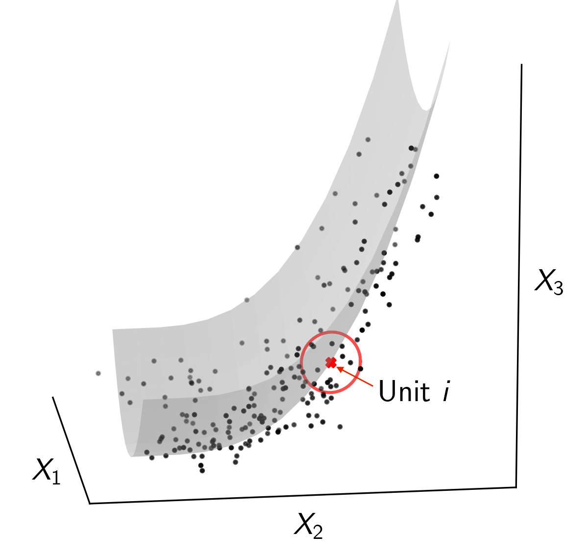
Figure 1: $K$-Nearest Neighbors Matching

Using the data of Acemoglu, Johnson, Kermani, Kwak, and Mitton (2016), I implement $K$-NN matching for each unit based on stock returns in the first 125 days with $K=127$. This relatively large $K$ is selected based on a data-driven procedure described in Step 2 in Section 3.2. Due to the noise in the measurements, choosing a small $K$ may not help reduce the resultant matching discrepancy (see discussions below Theorem 4.1). To have a sense of the performance of $K$-NN matching, I calculate for each unit the maximum distance of matched pairs divided by the standard deviation of the distance across all pairs, which can be viewed as a normalized matching discrepancy in terms of the observed returns. Table 1 reports some summary statistics for treated and control groups respectively. Matching performs well for treated units, whereas some control units are matched with someone relatively far away. In later analysis, I will check the robustness of the results by varying the number of nearest neighbors or dropping a few control units with large discrepancy.

Table 1: $K$-NN Matching: Maximum Distance of Matched Pairs

	Min.	1st Qu.	Median	Mean	3rd Qu.	Max.
Treated	$0.741$	$1.137$	$1.260$	$1.298$	$1.387$	$1.948$
Control	$0.673$	$0.957$	$1.147$	$1.314$	$1.440$	$6.813$

• Notes: For each unit, the maximum distance of matched pairs are normalized by dividing it by the standard deviation of the distance across all pairs.
  

Local Principal Component Analysis. This step makes use of the subsample labeled by $\ddagger$, i.e., the submatrix of $\bm{X}$ with row indices in $\mathcal{T}^{\ddagger}$. Given a set of nearest neighbors $\mathcal{N}_{i}$ from the previous step, define a $T^{\ddagger}\times K$ matrix $\bm{X}_{\langle i\rangle}=(\bm{X}^{\ddagger}_{\cdot j_{1}(i)},\cdots,\bm{X}^{\ddagger}_{\cdot j_{K}(i)})$. The subscript $\langle i\rangle$ indicates that the data matrix is defined locally for unit $i$. For these nearest neighbors, the unknown function $\eta_{t}(\cdot)$ can be locally approximated by a linear combination of some basis functions of latent variables. Then, $\bm{X}_{\langle i\rangle}$ admits a linear factor structure up to approximation errors:

$$\bm{X}_{\langle i\rangle}=\bm{F}_{\langle i\rangle}\bm{\Lambda}_{\langle i\rangle}^{\prime}+\bm{r}_{\langle i\rangle}+\bm{u}_{\langle i\rangle},$$ (3.2)

where $\bm{u}_{\langle i\rangle}=(\bm{u}^{\ddagger}_{\cdot j_{1}(i)},\cdots,\bm{u}^{\ddagger}_{\cdot j_{K}(i)})$. $\bm{F}_{\langle i\rangle}\bm{\Lambda}_{\langle i\rangle}^{\prime}+\bm{r}_{\langle i\rangle}$ is the possibly nonlinear factor component. The $K\times\mathsf{d}_{\lambda}$ matrix $\bm{\Lambda}_{\langle i\rangle}$ can be viewed as approximation basis functions of latent confounders (evaluated at the data points), the $T^{\ddagger}\times\mathsf{d}_{\lambda}$ matrix $\bm{F}_{\langle i\rangle}$ collects the corresponding coefficients, and $\bm{r}_{\langle i\rangle}$ is the resultant approximation error. The user-specified parameter $\mathsf{d}_{\lambda}$ governs the number of approximation terms. $\bm{F}_{\langle i\rangle}$ and $\bm{\Lambda}_{\langle i\rangle}$, referred to as factor and loading matrices respectively, can be identified up to a rotation and estimated by PCA (Bishop, 2006):

$$(\widehat{\bm{F}}_{\langle i\rangle},\widehat{\bm{\Lambda}}_{\langle i\rangle})=\underset{\scalebox{0.6}{ $\tilde{\bm{F}}_{\langle i\rangle}\in\mathbb{R}^{T^{\ddagger}\times\mathsf{d}_{\lambda}},\tilde{\bm{\Lambda}}_{\langle i\rangle}\in\mathbb{R}^{K\times\mathsf{d}_{\lambda}}$}}{\operatorname*{arg\,min}}\operatorname*{Tr}\Big{[}\Big{(}\bm{X}_{\langle i\rangle}-\tilde{\bm{F}}_{\langle i\rangle}\tilde{\bm{\Lambda}}_{\langle i\rangle}^{\prime}\Big{)}\Big{(}\bm{X}_{\langle i\rangle}-\tilde{\bm{F}}_{\langle i\rangle}\tilde{\bm{\Lambda}}_{\langle i\rangle}^{\prime})^{\prime}\Big{]}$$ (3.3)

such that $\frac{1}{T^{\ddagger}}\tilde{\bm{F}}_{\langle i\rangle}^{\prime}\tilde{\bm{F}}_{\langle i\rangle}=\bm{I}_{\mathsf{d}_{\lambda}}$ and $\frac{1}{K}\tilde{\bm{\Lambda}}_{\langle i\rangle}^{\prime}\tilde{\bm{\Lambda}}_{\langle i\rangle}$ is diagonal. Let $\widehat{\bm{\lambda}}_{\ell,\langle i\rangle}$ be the column in $\widehat{\bm{\Lambda}}_{\langle i\rangle}$ that corresponds to a generic unit $\ell$.

The idea underlying (3.3), i.e., applying PCA locally to neighbors of each unit, is similar to the step of learning local tangent spaces in Zhang and Zha (2004). The main difference is that $K$-NN matching and PCA in my procedure are conducted on different rows of $\bm{X}$. This is motivated by the fact that searching for nearest neighbors has implicitly used the information on $\{\bm{u}_{i}\}$. Without sample splitting across the $t$ dimension, for units within the same local neighborhood, the nonlinear factor components $\bm{F}_{\langle i\rangle}\bm{\Lambda}_{\langle i\rangle}+\bm{r}_{\langle i\rangle}$ would be correlated with the noise $\bm{u}_{\langle i\rangle}$, rendering the standard PCA technique inapplicable. Row-wise sample splitting is a simple remedy, when the noise is independent (or weakly dependent) across $t$. Note that splitting is not necessary if a researcher believes that $K$-NN matching suffices for later analysis.

The decomposition (3.2) is primarily of theoretical interest. In practice, there is no need to specify a particular approximation basis $\bm{\Lambda}_{\langle i\rangle}$ for implementing PCA as in (3.3). Also, the number of local principal components to be extracted ($\mathsf{d}_{\lambda}$) plays a similar role as the degree of the basis in local polynomial regression and can be set as a fixed number (independent of $n$ and $T$). Two strategies may be employed:

• Fixed-order approximation: given the number of latent variables $\mathsf{d}_{\alpha}$, choose $\mathsf{d}_{\lambda}$ accordingly so that approximation terms up to a certain order are extracted. For instance, when $\mathsf{d}_{\alpha}=2$, extract at least three leading local principal components to achieve local linear approximation. When $\mathsf{d}_{\alpha}$ is unknown, determine it using the strategy described later in Remark 4.5.

• Bias-minimizing approximation: given a set of nearest neighbors, investigate the magnitude of local eigenvalues in (3.3), and then extract all local principal components that are sufficiently strong to be differentiated from the noise. It is similar to the idea used in, e.g., Bai and Ng (2002) and Ahn and Horenstein (2013), which develop techniques for determining the number of factors in linear models. Consequently, the order of the approximation bias $\bm{r}_{\langle i\rangle}$ is no greater than that of the noise $\bm{\epsilon}_{\langle i\rangle}$ and cannot be further reduced by extracting more local principal components.

Note that whichever strategy is used, we can at most achieve the approximation power such that the order of approximation bias does not exceed that of the noise. See more discussion about determining $\mathsf{d}_{\lambda}$ in Remark 4.6.

The idea of local PCA is illustrated in Figure 2. Units around the red dot are approximately lying on a (local) linear tangent plane. Intuitively, this approximation is analogous to the local linear regression in the nonparametrics literature, though conditioning variables in this context are unobserved. More generally, if more leading factors can be differentiated from the noise, a local nonlinear principal subspace can be constructed for a higher-order approximation of the underlying surface.

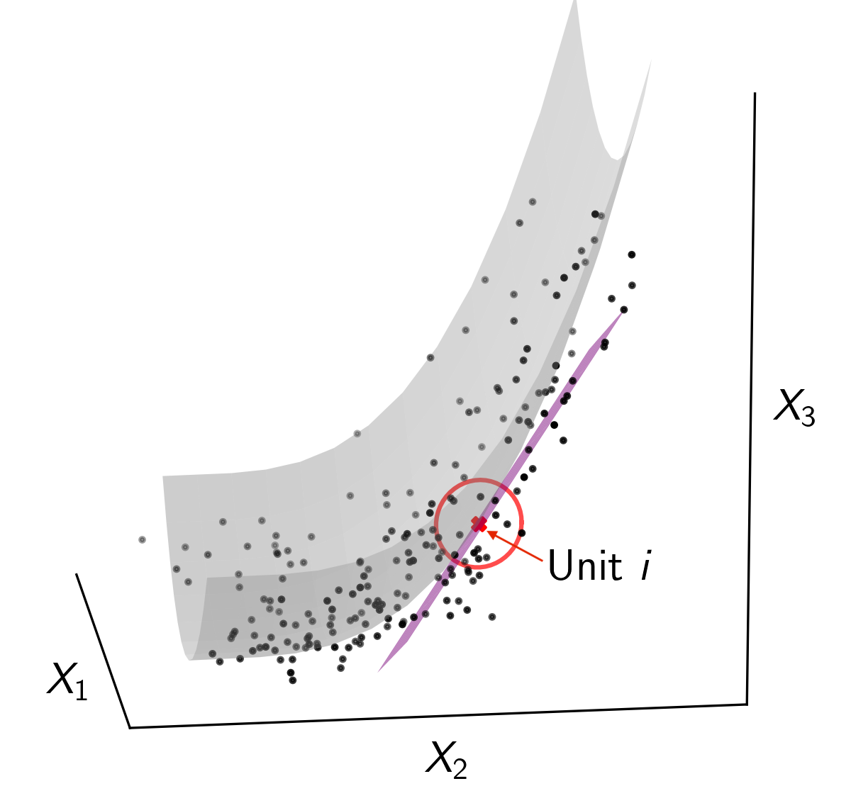
Figure 2: Local Tangent Space Approximation

Using the data of Acemoglu, Johnson, Kermani, Kwak, and Mitton (2016), I implement local PCA for each unit. Recall that for each firm a set of nearest neighbors has been obtained using the stock returns in the first $125$ days. PCA can be conducted for this subgroup of firms using their stock returns in the next 125 days. Figure 3 shows several leading eigenvalues corresponding to the neighborhood for a particular unit (“AMERICAN EXPRESS CO.”), suggesting that extracting one or two local principal components is a reasonable choice. In the subsequent analysis, I set $\mathsf{d}_{\lambda}=1$. Results based on $\mathsf{d}_{\lambda}=2$ are similar and omitted to conserve space.

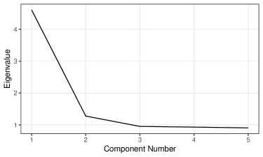
Figure 3: Local Eigenvalues for One Neighborhood

3.2 Step 2: Factor-Augmented Regression

For the outcome equation (2.1), the predicted value $\widehat{\varsigma}_{i,\jmath}$ for unit $i$ is given by

$$\begin{split}\widehat{\varsigma}_{i,\jmath}=\bm{z}_{i}^{\prime}\widehat{\bm{\beta}}_{\jmath,\langle i\rangle}+\widehat{\mu}_{\jmath}(\bm{\alpha}_{i}),\quad\widehat{\mu}_{\jmath}(\bm{\alpha}_{i})=\widehat{\bm{\lambda}}_{i,\langle i\rangle}^{\prime}\widehat{\bm{b}}_{\jmath,\langle i\rangle},\quad\text{where}\\[10.00002pt] (\widehat{\bm{\beta}}_{\jmath,\langle i\rangle}^{\prime},\;\widehat{\bm{b}}_{\jmath,\langle i\rangle}^{\prime})^{\prime}=\operatorname*{arg\,max}_{(\bm{\beta}^{\prime},\bm{b}^{\prime})^{\prime}\in\mathbb{R}^{\mathsf{d}_{z}+\mathsf{d}_{\lambda}}}\;\sum_{\ell\in\mathcal{N}_{i}}d_{\ell}(\jmath)(y_{\ell}-\bm{z}_{\ell}^{\prime}\bm{\beta}-\widehat{\bm{\lambda}}_{\ell,\langle i\rangle}^{\prime}\bm{b})^{2}.\end{split}$$ (3.4)

It can be viewed as a local least squares regression with generated regressors $\widehat{\bm{\lambda}}_{\ell,\langle i\rangle}$. The treatment equation (2.2) can be treated exactly the same way. By regressing $d_{\ell}(\jmath)$ on $\bm{z}_{\ell}$ and $\widehat{\bm{\lambda}}_{\ell,\langle i\rangle}$ for $\ell\in\mathcal{N}_{i}$, one can obtain the predicted value $\widehat{p}_{i,\jmath}$. Note that as discussed in Section 5.3 below, other approaches such as nonparametric logit or probit regression can also be employed to estimate these propensity scores.

In practice, I suggest taking $\mathsf{d}_{\lambda}$ as a fixed number and choosing the tuning parameter $K$ accordingly. For instance, we can focus on the subgroup at the treatment level $\jmath$, and let $\mathsf{d}_{\lambda}=\mathsf{d}_{\alpha}+1$ to achieve the same approximation power of local linear estimation. Then, $K$ can be chosen possibly through two strategies:

• Cross validation. Split all units (in this subgroup) into several parts. In each round, use one part as the testing sample and other data as the training sample. For each unit in the testing sample, search for $K$ nearest neighbors and implement local PCA using the training sample, and then obtain the prediction $\widehat{\varsigma}_{i,\jmath}$ accordingly. The goal is to choose $K$ that minimizes the cross-validation estimate of the prediction error. See Section SA-5.3.1 of the SA for more details.

• Direct plug-in (DPI). The goal is to choose $K$ that minimizes the integrated mean squared error of $\widehat{\varsigma}_{i,\jmath}$. Given the results in Theorem 4.4 below, we can take a DPI choice $\widehat{K}_{\mathtt{DPI}}=[(\frac{\mathsf{d}_{\alpha}\widehat{\mathscr{V}}}{4\widehat{\mathscr{B}}})^{\frac{\mathsf{d}_{\alpha}}{4+\mathsf{d}_{\alpha}}}n^{\frac{4}{4+\mathsf{d}_{\alpha}}}]$, where $\widehat{\mathscr{B}}$ and $\widehat{\mathscr{V}}$ are some estimates corresponding to the integrated (squared) bias and the integrated variance and $[\cdot]$ denotes a rounding operator. In practice, one can obtain $\widehat{\mathscr{B}}$ and $\widehat{\mathscr{V}}$ by choosing an initial $K$ and implementing estimation procedures similar to that in Step 1 and 2. See Section SA-5.3.2 of the SA for more details.

For the purpose of illustration, I implement a local regression of stock returns at date $t$ on the leading factor loading extracted previously, for each $t=-20,\cdots,0,1$, where $t=0$ denotes the day when the treatment starts. Figure 4(a) shows the fitted values in black and the observed daily returns in grey for the $22$ treated firms, and the result for American Express Co. is displayed in Figure 4(b). Recall that the fitted values are the estimates of conditional expectations of stock returns without treatment given the latent variables. Clearly, after day $0$, many sequences of stock returns increase sharply compared with the corresponding fitted values.

Figure 4: Local Least Squares: Stock Returns

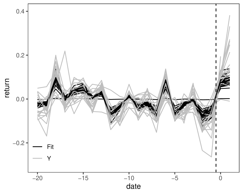
(a) All Treated Firms

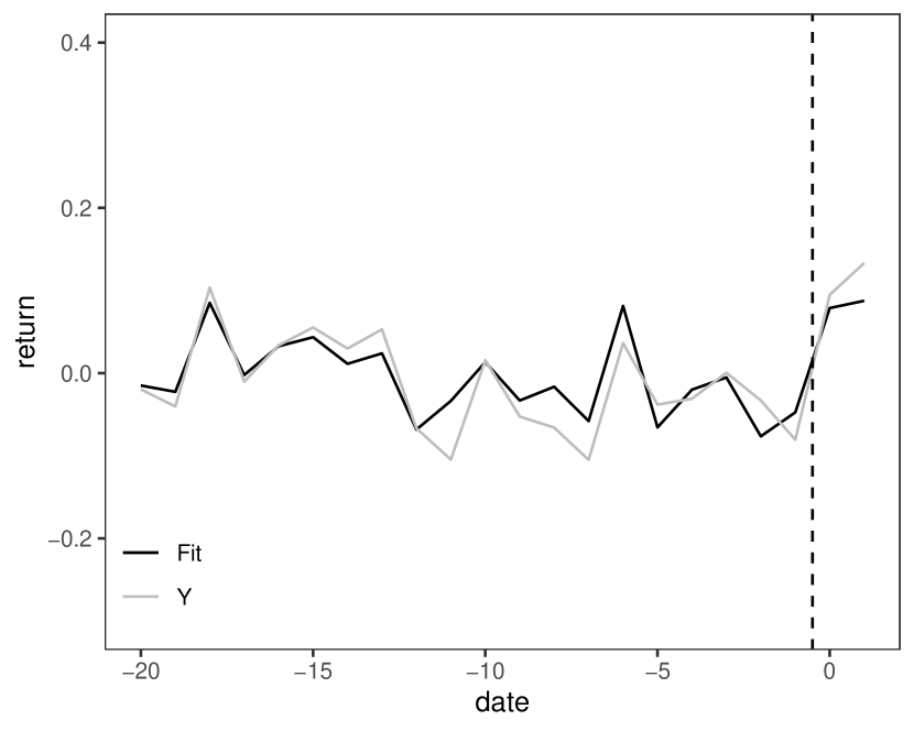
(b) American Express Co.

3.3 Step 3: Counterfactual Analysis

The final step is to estimate the counterfactual means of potential outcomes, which forms the basis of estimators for other causal parameters. Specifically, consider $\theta_{\jmath,\jmath^{\prime}}:=\mathbb{E}[y_{i}(\jmath)|s_{i}=\jmath^{\prime}]$. Let $p_{\ell}=\mathbb{P}(s_{i}=\ell)$ for any $\ell\in\mathcal{J}$. Under unconfoundedness conditional on $\bm{z}_{i}$ and $\bm{\alpha}_{i}$ (see Assumption 1 below),

$$\theta_{\jmath,\jmath^{\prime}}=\mathbb{E}\left[\frac{d_{i}(\jmath^{\prime})\varsigma_{i,\jmath}}{p_{\jmath^{\prime}}}+\frac{p_{i,\jmath^{\prime}}}{p_{\jmath^{\prime}}}\frac{d_{i}(\jmath)(y_{i}-\varsigma_{i,\jmath})}{p_{i,\jmath}}\right].$$

An estimator of $\theta_{\jmath,\jmath^{\prime}}$ is given by

$$\widehat{\theta}_{\jmath,\jmath^{\prime}}:=\frac{1}{n}\sum_{i=1}^{n}\left[\frac{d_{i}(\jmath^{\prime})\widehat{\varsigma}_{i,\jmath}}{\widehat{p}_{\jmath^{\prime}}}+\frac{\widehat{p}_{i,\jmath^{\prime}}}{\widehat{p}_{\jmath^{\prime}}}\frac{d_{i}(\jmath)(y_{i}-\widehat{\varsigma}_{i,\jmath})}{\widehat{p}_{i,\jmath}}\right],$$ (3.5)

where $\widehat{\varsigma}_{i,\jmath}$, $\widehat{p}_{i,\jmath}$ and $\widehat{p}_{i,\jmath^{\prime}}$ are obtained in the second step, and $\widehat{p}_{\ell}=\frac{1}{n}\sum_{i=1}^{n}d_{i}(\ell)$ for $\ell=\jmath,\jmath^{\prime}$. For the purpose of inference, a simple plug-in variance estimator for $\widehat{\theta}_{\jmath,\jmath^{\prime}}$ is

$$\widehat{\sigma}_{\jmath,\jmath^{\prime}}^{2}:=\frac{1}{n}\sum_{i=1}^{n}\bigg{[}\frac{d_{i}(\jmath^{\prime})(\widehat{\varsigma}_{i,\jmath}-\widehat{\theta}_{\jmath,\jmath^{\prime}})^{2}}{\widehat{p}_{\jmath^{\prime}}^{2}}\bigg{]}+\frac{1}{n}\sum_{i=1}^{n}\bigg{[}\frac{\widehat{p}_{i,\jmath^{\prime}}^{2}d_{i}(\jmath)(y_{i}-\widehat{\varsigma}_{i,\jmath})^{2}}{\widehat{p}_{\jmath^{\prime}}^{2}\widehat{p}^{2}_{i,\jmath}}\bigg{]}$$ (3.6)

One may expect $\sqrt{n}\widehat{\sigma}_{\jmath,\jmath^{\prime}}^{-1}(\widehat{\theta}_{\jmath,\jmath^{\prime}}-\theta_{\jmath,\jmath^{\prime}})\rightsquigarrow\mathsf{N}(0,1)$, which will be shown in Theorem 4.5 below. Confidence intervals and hypothesis testing procedures can be constructed accordingly.

Estimators of other parameters may be constructed in a similar way or based on $\{\widehat{\theta}_{\jmath,\jmath^{\prime}}\}_{\jmath,\jmath^{\prime}\in\mathcal{J}}$. For example, the average treatment effect on the treatment group $\jmath^{\prime}=\ell$ compared to the baseline treatment status $\jmath=0$ can be estimated by $\widehat{\theta}_{\ell,\ell}-\widehat{\theta}_{0,\ell}$ where $\widehat{\theta}_{\ell,\ell}=\sum_{i=1}^{n}d_{i}(\ell)y_{i}/\sum_{i=1}^{n}d_{i}(\ell)$.

As an illustration, I estimate the average treatment effect of Geithner connections on cumulative returns from day 0 to day 1 (CAR[0,1]) for firms with connections. Since the number of treated units is relatively small, the propensity score is obtained by taking a simple local average within each local neighborhood. For the outcome equation, I run a local regression of stock returns of firms with no connections on the factor loading extracted previously ($\mathsf{d}_{\lambda}=1$). Different choices of $K$ are considered, which correspond to $K=Cn^{2/3}$ where $C=0.5,1,2$, and I also use the strategy outlined in Section SA-5.3 of the SA to obtain a DPI choice $\widehat{K}_{\mathtt{DPI}}$ based on an initial choice $K=2n^{2/3}$. Assuming there exists one latent variable, such choices coincide with the mean squared error (MSE) optimal rate of the underlying nonparametric estimators. The above procedure is applied to the full sample and a base sample. The latter, as defined in Acemoglu, Johnson, Kermani, Kwak, and Mitton (2016), excludes firms whose returns are highly correlated with Citigroup.

Results are reported in the first two columns of Table 2. I also include two results based on synthetic matching in Acemoglu, Johnson, Kermani, Kwak, and Mitton (2016) and one result based on a penalized synthetic control method in Abadie and L’Hour (2021). To make these results comparable, I report the 95% confidence intervals for hypothesis testing of the average treatment effect (on the treated) being equal to zero (numbers in brackets in Table 2), but note that the underlying assumptions and inference methodology of the other two papers are different from mine. The estimated average cumulative abnormal return for the connected firms using the proposed method ranges from $0.065$ to $0.105$ and significantly differs from zero at the $0.05$ level. I also check the robustness of the results by excluding firms in the control group with large normalized matching discrepancy (top $10\%$ in Table 1). Results are similar and omitted to conserve space.

The analysis so far has controlled for latent variables only. Three additional covariates are available in the dataset of Acemoglu, Johnson, Kermani, Kwak, and Mitton (2016): firm size (log of total assets), profitability (return on equity), and leverage (total debt to total capital) as of 2008. They can be incorporated into the local least squares regression in Step 2 as additional regressors $\bm{z}_{i}$. Results are reported in the third and fourth columns of Table 2. The estimated effect is slightly smaller than that without additional covariates, but still significant at the 0.05 level.

Table 2: Average Treatment Effect of Connections on the Treated

	No Covariates			Add Covariates
	Full Sample	Base Sample		Full Sample	Base Sample
Local PCA, $K=$
34	0.095	0.081		0.085	0.069
	[-0.054, 0.054]	[-0.049, 0.049]		[-0.054, 0.054]	[-0.064, 0.064]
69	0.098	0.091		0.077	0.065
	[-0.052, 0.052]	[-0.051, 0.051]		[-0.051, 0.051]	[-0.049, 0.049]
139	0.105	0.096		0.089	0.078
	[-0.054, 0.054]	[-0.053, 0.053]		[-0.053, 0.053]	[-0.050, 0.050]
$\widehat{K}_{\mathtt{DPI}}$	0.103	0.095		0.090	0.078
	[-0.054, 0.054]	[-0.053, 0.053]		[-0.053, 0.053]	[-0.050, 0.050]
Acemoglu et al. (2016)
Estimate	0.005	0.060		-	-
CI for TE=0	[-0.029, 0.014]	[-0.068, 0.036]		-	-
Abadie and L’Hour (2021)
Estimate	-	0.061		-	-
CI for TE=0	-	[-0.050, 0.061]		-	-

• Notes: CAR[0,1] is the cumulative abnormal return from day 0 to day 1. The base sample excludes firms highly correlated with Citigroup. The numbers in brackets are the 95% confidence intervals for hypothesis testing of the effect of connections being equal to zero. The DPI choices $\widehat{K}_{\mathtt{DPI}}$ in the four columns are $127$, $134$, $128$ and $135$ respectively.
  

4 Main Results

4.1 Assumptions

I begin with unconfoundedness and overlap conditions commonly used in the causal inference literature. Note that the conditioning variables $\bm{\alpha}_{i}$ in this scenario are unobservable.

Assumption 1 (Unconfoundedness and Overlap).

$\{(y_{i},s_{i},\bm{z}_{i},\bm{\alpha}_{i})\}_{i=1}^{n}$ is i.i.d over $1\leq i\leq n$ and satisfies that (a) $y_{i}(\jmath)\mathchoice{\mathrel{\hbox to0.0pt{$\displaystyle\perp$\hss}\mkern 2.0mu{\displaystyle\perp}}}{\mathrel{\hbox to0.0pt{$\textstyle\perp$\hss}\mkern 2.0mu{\textstyle\perp}}}{\mathrel{\hbox to0.0pt{$\scriptstyle\perp$\hss}\mkern 2.0mu{\scriptstyle\perp}}}{\mathrel{\hbox to0.0pt{$\scriptscriptstyle\perp$\hss}\mkern 2.0mu{\scriptscriptstyle\perp}}}d_{i}(\jmath^{\prime})|\bm{z}_{i},\bm{\alpha}_{i}$, $\forall\jmath,\jmath^{\prime}\in\mathcal{J}$; (b) for all $\jmath\in\mathcal{J}$, $\mathbb{P}(s_{i}=\jmath|\bm{z}_{i},\bm{\alpha}_{i})\geq p_{\min}>0$ for almost surely $\bm{\alpha}_{i}$.

The next assumption imposes mild regularity conditions on the treatment effects model and the latent structure of $\bm{x}_{i}$.

Assumption 2 (Regularities).

Let $\bar{m}\geq 2$ and $\nu>0$ be some constants. Equations (2.1), (2.2) and (2.6) hold with the following conditions satisfied:

1. For all $\jmath\in\mathcal{J}$, $\mu_{\jmath}(\cdot),\rho_{\jmath}(\cdot)$ are $\bar{m}$-times continuously differentiable.

2. $\bm{z}_{i}$ has a compact support and $\mathbb{E}[\tilde{\bm{z}}_{i}\tilde{\bm{z}}_{i}^{\prime}|\bm{\alpha}_{i}]>0$ a.s. for $\tilde{\bm{z}}_{i}=\bm{z}_{i}-\mathbb{E}[\bm{z}_{i}|\bm{\alpha}_{i}]$. Conditional on $\mathcal{F}$, $\{(\bm{\epsilon}_{i},\bm{v}_{i})\}_{i=1}^{n}$ are independent across $i$ with zero means and independent of $\{\bm{x}_{i}\}_{i=1}^{n}$. Also, $\max_{1\leq i\leq n}\mathbb{E}[\|\bm{\epsilon}_{i}\|_{2}^{2+\nu}|\mathcal{F}]<\infty$ and $\max_{1\leq i\leq n}\mathbb{E}[\|\bm{v}_{i}\|_{2}^{2+\nu}|\mathcal{F}]<\infty$ a.s. on $\mathcal{F}$.

3. $\{\bm{\alpha}_{i}\}_{i=1}^{n}$ has a compact convex support $\mathcal{A}$ with a density bounded and bounded away from zero.

4. For all $1\leq t\leq T$, $\eta_{t}(\cdot)$ is $\bar{m}$-times continuously differentiable with all partial derivatives of order no greater than $\bar{m}$ bounded by a universal constant.

5. Conditional on $\mathcal{F}$, $\{u_{it}:1\leq i\leq n,1\leq t\leq T\}$ is independent across $i$ and over $t$, and $\max_{1\leq i\leq n,1\leq t\leq T}\mathbb{E}[|u_{it}|^{2+\nu}|\mathcal{F}]<\infty$ a.s. on $\mathcal{F}$.

Parts (a), (b), and (c) concern the regularities of the treatment effects model characterized by Equations (2.1) and (2.2). The conditional expectations of potential outcomes and propensity scores are sufficiently smooth functions, and other standard conditions are imposed on the conditioning variables and errors. Regarding the latent structure of $\bm{x}_{i}$ described in Equation (2.6), part (d) ensures that all latent functions belong to a Hölder class of order $\bar{m}$, and part (e) are standard conditions on errors commonly used in factor analysis and graphon estimation. The constant $\bar{m}$ governs the smoothness of unknown functions, and $\nu$ controls the tails of error terms. They are assumed to be the same across Equations (2.1)-(2.6) only for simplicity.

Recall that the main task of the first step is to learn $\bm{\alpha}_{i}$ from $\bm{x}_{i}$. $\bm{\alpha}_{i}$ is not identifiable, but it is unnecessary to identify it in an exact sense since only predictions based on $\bm{\alpha}_{i}$ matter for the main analysis. Intuitively, the goal is to extract local geometric relations among latent $\bm{\alpha}_{i}$’s, which are reflected by index sets for nearest neighbors and local factor loadings described in Section 3. The next three assumptions detail the restrictions on the latent nonlinear structure generated by $\{\eta_{t}(\cdot)\}_{t=1}^{T}$, ensuring that the relations learned from $\bm{x}_{i}$’s can be translated into that for $\bm{\alpha}_{i}$’s.

Assumption 3 below can be intuitively understood as an “identification” condition for $\bm{\alpha}_{i}$. It implies that the difference in $\bm{\alpha}_{i}$ can be revealed by the observed measurements $\bm{x}_{i}$ as the dimensionality of $\bm{x}_{i}$ grows large, though exact identification of $\bm{\alpha}_{i}$ is impossible without further restrictions. Due to the row-wise sample splitting, I will write $\bm{\eta}^{\dagger}(\cdot):=(\eta_{t}(\cdot))_{t\in\mathcal{T}^{\dagger}}$, and $\bm{\eta}^{\ddagger}(\cdot):=(\eta_{t}(\cdot))_{t\in\mathcal{T}^{\ddagger}}$, which are $T^{\dagger}\times 1$ and $T^{\ddagger}\times 1$ column vectors of latent functions respectively.

Assumption 3 (Latent Structure: Identification).

For every $\varepsilon>0$,

$$\lim_{\Delta\rightarrow 0}\limsup_{n,T^{\dagger}\rightarrow\infty}\;\mathbb{P}\Big{\{}\max_{1\leq i\leq n}\;\max_{j:\mathfrak{d}_{\infty}(\bm{\eta}^{\dagger}(\bm{\alpha}_{i}),\bm{\eta}^{\dagger}(\bm{\alpha}_{j}))<\Delta}\;\|\bm{\alpha}_{i}-\bm{\alpha}_{j}\|_{2}>\varepsilon\Big{\}}=0.$$ (4.1)

When this condition holds, units within the same neighborhood obtained by matching on the large-dimensional $\bm{x}_{i}$ (see Step 1 in Section 3) are similar in terms of the latent $\bm{\alpha}_{i}$. Otherwise, units with quite different values of $\bm{\alpha}_{i}$ could be matched.

The idea underlying this assumption is related to the completeness condition widely used in econometric identification problems (Newey and Powell, 2003; Chernozhukov and Hansen, 2005; Hu and Schennach, 2008). Roughly speaking, for a family of distributions, completeness requires that the density of a variable sufficiently vary across different values of the conditioning variable. Analogously, condition (4.1) amounts to saying that there is enough variation observed on the latent surface for different values of the latent variables.

Remark 4.1 (Plausibility of Assumption 3).

Assumption 3 is a fundamental requirement for informativeness of measurements. To get a sense of its plausibility, consider a linear factor model with an intercept: $\eta_{t}(\alpha_{i})=c_{0}+\varpi_{t}\alpha_{i}$ for $c_{0}$, $\varpi_{t}\in\mathbb{R}$. When $\varpi_{t}\neq 0$ if and only if $t=1$ (the factor is too “sparse”), most measurements in $\bm{x}_{i}$ are uninformative about $\alpha_{i}$. For $\alpha_{i}\neq\alpha_{j}$, their difference is revealed only when $t=1$. The distance between $\bm{\eta}^{\dagger}(\alpha_{i})$ and $\bm{\eta}^{\dagger}(\alpha_{j})$ becomes negligible as $T$ diverges, which violates condition (4.1). However, as long as a non-negligible subset of $\{\varpi_{t}\}_{t\in\mathcal{T}^{\dagger}}$ are nonzero, the corresponding measurements suffice to differentiate the two units. In other words, the proposed method only requires some but not all measurements to be informative, and importantly, it is unnecessary to know their identities a priori. The large-dimensional measurements are automatically aggregated to derive information on the latent confounders. Section SA-2.3 of the SA provides more examples other than the linear factor model that satisfy Assumption 3. $\lrcorner$

Remark 4.2 (Other Metrics).

Assumption 3 can be further generalized by specifying a generic metric $\mathfrak{d}(\cdot,\cdot)$. For instance, define a possibly vector-valued function $\bm{h}_{i}:\mathbb{R}^{T^{\dagger}}\mapsto\mathbb{R}^{\mathsf{d}_{h}}$ that transforms the observed measurements $\bm{X}_{\cdot i}^{\dagger}$ into a $\mathsf{d}_{h}$-vector of “new” features $\bm{h}_{i}(\bm{X}_{\cdot i})$, and conduct $K$-NN matching on the transformed features in terms of the Euclidean norm. In this case, the distance between units $i$ and $j$ is given by

$$\mathfrak{d}(\bm{X}_{\cdot i}^{\dagger},\bm{X}_{\cdot j}^{\dagger})=\|\bm{h}_{i}(\bm{X}_{\cdot i}^{\dagger})-\bm{h}_{j}(\bm{X}_{\cdot j}^{\dagger})\|_{2}.$$

In practice, introducing such transformations may be useful since it allows for rescaling or reweighting different measurements to obtain features that are more informative about latent confounders.

This general informativeness requirement also covers the injective moment condition in Bonhomme, Lamadon, and Manresa (2021) as a special case (see Assumption 2 therein). It relies on a particular choice of the transformation $\bm{h}_{i}(\cdot)$ such that $\bm{h}_{i}(\bm{X}_{i}^{\dagger})$ converges to $\bm{\varphi}(\bm{\alpha}_{i})$ for some fixed function $\bm{\varphi}(\cdot)$. In some scenarios, an informativeness condition based on such a choice may be too stringent. For example, consider a linear factor model with $\eta_{t}(\alpha_{i})=\varpi_{t}\alpha_{i}$ and let $\bm{h}_{i}(\bm{X}_{\cdot i}^{\dagger})=\frac{1}{T^{\dagger}}\sum_{j=1}^{T^{\dagger}}\bm{X}_{\cdot i}^{\dagger}$. The transformed features $\bm{h}_{i}(\bm{X}_{\cdot i}^{\dagger})$ is uninformative if $\frac{1}{T^{\dagger}}\sum_{t=1}^{T^{\dagger}}\varpi_{t}\rightarrow_{\mathbb{P}}0$. By contrast, as explained in Remark 4.1, as long as there are a fraction of $\{\varpi_{t}\}_{t=1}^{\dagger}$ is nonzero, the difference in latent features can still be revealed by the proposed strategy. $\lrcorner$

The next assumption concerns the non-collinearity of derivatives of latent functions, which facilitates the quantification of indirect matching and local PCA.

Assumption 4 (Latent Structure: Non-degeneracy).

For some $\underline{c}>0$ and $2\leq m\leq\bar{m}$,

$$\begin{array}[]{r@{}l}&\underset{n,T^{\dagger}\rightarrow\infty}{\lim}\;\mathbb{P}\bigg{\{}\underset{1\leq i\leq n}{\min}s_{\min}\Big{(}\frac{1}{T^{\dagger}}\underset{t\in\mathcal{T}^{\dagger}}{\sum}(\mathscr{D}^{[m-1]}\bm{\eta}_{t}(\bm{\alpha}_{i}))(\mathscr{D}^{[m-1]}\bm{\eta}_{t}(\bm{\alpha}_{i}))^{\prime}\Big{)}\geq\underline{c}\bigg{\}}=1,\\ &\underset{n,T^{\ddagger}\rightarrow\infty}{\lim}\;\mathbb{P}\Big{\{}\underset{1\leq i\leq n}{\min}s_{\min}\bigg{(}\frac{1}{T^{\ddagger}}\underset{t\in\mathcal{T}^{\ddagger}}{\sum}(\mathscr{D}^{[m-1]}\bm{\eta}_{t}(\bm{\alpha}_{i}))(\mathscr{D}^{[m-1]}\bm{\eta}_{t}(\bm{\alpha}_{i}))^{\prime}\Big{)}\geq\underline{c}\bigg{\}}=1.\end{array}$$ (4.2)

Assumption 4 ensures that the derivatives of latent functions up to order $m-1$ are not too collinear. It is analogous to the non-degenerate factors condition commonly imposed in linear factor analysis (see, e.g., Bai, 2003, 2009).

Remark 4.3 (Plausibility of Assumption 4).

Intuitively, Assumption 4 says that the linearity or nonlinearity of latent functions in $\bm{\alpha}_{i}$ characterized by the corresponding derivatives exists. Again, to get a sense of its plausibility, consider the linear factor model discussed before: $\eta_{t}(\alpha_{i})=c_{0}+\varpi_{t}\alpha_{i}$. (4.2) reduces to the requirement that $\frac{1}{T^{\dagger}}\sum_{t\in\mathcal{T}^{\dagger}}(c_{0}+\varpi_{t}\alpha_{i},\varpi_{t})^{\prime}(c_{0}+\varpi_{t}\alpha_{i},\varpi_{t})$ has the minimum eigenvalue bounded away from zero for all $1\leq i\leq n$. It holds if $c_{0}\neq 0$ and $\varpi_{t}$ varies sufficiently across $t$. Note that when $c_{0}=0$, (4.2) still holds if the “zeroth” derivative $\nabla^{0}\eta_{t}(\bm{\alpha}_{i})$ is dropped from $\mathscr{D}^{m-1}\bm{\eta}_{t}(\bm{\alpha}_{i})$ and $\frac{1}{T^{\dagger}}\sum_{t\in\mathcal{T}^{\dagger}}\varpi_{t}^{2}\gtrsim 1$. The theory of this paper can still be established in this scenario. In fact, Assumption 4 is only one primitive condition that links the linearity or nonlinearity of latent functions with the non-degenerate factors in my model. Section SA-2 of the SA provides a set of high-level conditions directly imposed on the approximation (3.2), allowing for potential degeneracy of some derivatives in $\mathscr{D}^{(m-1)}\bm{\eta}_{t}(\bm{\alpha}_{i})$. In this sense, my theory covers the usual linear factor model as a special case rather than excludes it. Also, see Section SA-2.3 of the SA for more examples other than the linear factor model that satisfy Assumption 4. $\lrcorner$

The last assumption on the latent structure, which I refer to as non-collapsing, permits accurate translation from the matching discrepancy of observables to that of unobservables. Specifically, let $\mathscr{P}_{\bm{\alpha}_{0}}[\cdot]$ be the projection operator onto the $\mathsf{d}_{\alpha}$-dimensional space (embedded in $\mathbb{R}^{T^{\dagger}}$) spanned by the local tangent basis at $\bm{\eta}^{\dagger}(\bm{\alpha}_{0})$, i.e., $\nabla\bm{\eta}^{\dagger}(\bm{\alpha}_{0})$. Take an orthogonalized basis of this tangent space. Denote by $\mathscr{P}_{\bm{\alpha}_{0},\ell}[\cdot]$ the projection operator onto the $\ell$th direction of the tangent space. Then, $\mathscr{P}_{\bm{\alpha}_{0},\ell}[\bm{\eta}^{\dagger}(\bm{\alpha})]$ is the projection of $\bm{\eta}^{\dagger}(\bm{\alpha})$ onto the $\ell$th direction of the tangent space at $\bm{\eta}^{\dagger}(\bm{\alpha}_{0})$.

Assumption 5 (Latent Structure: Non-collapsing).

There exists an absolute constant $\underline{c}^{\prime}>0$ such that

$$\lim_{n,T^{\dagger}\rightarrow\infty}\;\mathbb{P}\Big{\{}\min_{1\leq\ell\leq\mathsf{d}_{\alpha}}\min_{1\leq i\leq n}\sup_{\bm{\alpha}\in\mathcal{A}}\frac{1}{T^{\dagger}}\Big{\|}\mathscr{P}_{\bm{a}_{i},\ell}[\bm{\eta}^{\dagger}(\bm{\alpha})]\Big{\|}_{2}^{2}\geq\underline{c}^{\prime}\Big{\}}=1.$$ (4.3)

Though seemingly involved at first glance, condition (4.3) has an intuitive geometric interpretation. Note that the latent functions $\{\eta_{t}(\cdot)\}_{t\in\mathcal{T}^{\dagger}}$ generate a $\mathsf{d}_{\alpha}$-dimensional surface embedded in $\mathbb{R}^{T^{\dagger}}$, and thus (4.3) simply says that if the whole surface is projected onto the tangent space at any data point, the dimensionality of the projection does not drop, as implied by the name “non-collapsing”.

Remark 4.4 (Plausibility of Assumption 5).

To get a sense of the plausibility of Assumption 5, consider the linear factor model: $\eta_{t}(\alpha_{i})=c_{0}+\varpi_{t}\alpha_{i}$. (4.3) is satisfied if $\frac{1}{T^{\dagger}}\sum_{t\in\mathcal{T}^{\dagger}}\varpi_{t}^{2}\asymp 1$ and the support $\mathcal{A}$ contains at least one $\alpha$ such that $|\alpha+(\frac{1}{T^{\dagger}}\sum_{t\in\mathcal{T}^{\dagger}}\varpi_{t}^{2})^{-1}(\frac{1}{T^{\dagger}}\sum_{t\in\mathcal{T}^{\dagger}}\varpi_{t}c_{0})|\geq C$ for some constant $C>0$. When $c_{0}=0$, the second restriction further reduces to the mild requirement that there exists one $\alpha$ with strictly positive absolute value. Intuitively, (4.3) holds if the factor ($\varpi_{t}$) is not degenerate or explosive and the dataset has some variation in the latent variable $\alpha_{i}$. Also, see Section SA-2.3 of the SA for more examples other than the linear factor model that satisfy Assumption 5. $\lrcorner$

Assumptions 3-5 are a group of lower-level conditions. The cornerstone of the proposed method is a local principal subspace approximation procedure, which has broad applicability and can be justified under higher-level conditions. In particular, the analysis below can be easily adapted to cover semi-strong factor models (Wang and Fan, 2017). See Section SA-2.2 of the SA for details.

4.2 Theoretical Results

Throughout the analysis below, I write $\delta_{KT}=(K^{1/2}\wedge T^{1/2})/\sqrt{\log(n\vee T)}$ and $h_{K,\alpha}=(K/n)^{1/\mathsf{d}_{\alpha}}$. Recall that $K$ is the number of nearest neighbors and $T$ is the dimensionality of $\bm{x}_{i}$. The asymptotic analysis is conducted assuming both $K$ and $T$ diverge as $n\rightarrow\infty$. As explained before, I use $\mathfrak{d}(\cdot,\cdot)=\mathfrak{d}_{\infty}(\cdot,\cdot)$. Moreover, $\mathsf{d}_{\lambda}$ is the number of extracted leading local principal components. I assume that $\mathsf{d}_{\lambda}=\binom{m-1+\mathsf{d}_{\alpha}}{\mathsf{d}_{\alpha}}$ so that the local approximation terms up to order $(m-1)$ for $\{\eta_{t}(\cdot)\}$ are extracted.

Latent Structure

I begin with the covariate equation (2.6) and provide some important intermediate results that may be of independent interest. More detailed results are given in Section SA-2 of the SA. The first theorem concerns the discrepancy of latent variables induced by matching on the observed measurements.

Theorem 4.1 (Indirect Matching).

Suppose that Assumptions 2(c), 2(d), 2(e), 3, 4 and 5 hold. If $\frac{n^{\frac{4}{\nu}}(\log n)^{\frac{\nu-2}{\nu}}}{T}\lesssim 1$, then,

$$\max_{1\leq i\leq n}\max_{1\leq k\leq K}\|\bm{\alpha}_{i}-\bm{\alpha}_{j_{k}(i)}\|_{2}\lesssim_{\mathbb{P}}(K/n)^{1/\mathsf{d}_{\alpha}}+\sqrt{\log n/T}.$$

As shown in the above theorem, the matching can be made up to errors consisting of two terms in an asymptotic sense. The first part $(K/n)^{1/\mathsf{d}_{\alpha}}$ reflects the direct matching discrepancy for $\bm{\alpha}_{i}$. It grows quickly with the number of latent variables, which coincides with the results in the nearest neighbors matching literature (Györfi, Kohler, Krzyzak, and Walk, 2002). The second term $\sqrt{\log n/T}$ arises from the existence of $\bm{u}_{i}$. By construction of the distance metric, averaging across the $t$ dimension can shrink the impact of $\bm{u}_{i}$ to the order of $T^{-1/2}$ up to a log penalty.

Note that if $\bm{\alpha}_{i}$ were observed, matching could be directly implemented on it with the number of matches $K$ fixed, and large-sample properties of the resultant matching estimators have been established in Abadie and Imbens (2006). In this paper, however, $\bm{\alpha}_{i}$ is unobservable, and matching can only be done on their noisy measurements, leading to the indirect matching discrepancy characterized by the second term in Theorem 4.1. Using a fixed (or small) number of nearest neighbors is unable to further reduce bias and thus is not recommended in this scenario.

The rate restriction in Theorem 4.1 is exploited in application of maximal inequalities, which ensures uniform convergence of sample averages across $t$. It becomes more relaxed when more stringent moment conditions (larger $\nu$) hold. In addition, as explained earlier, Assumption 5 is used to derive a sharp bound on the indirect matching discrepancy when $\mathfrak{d}_{\infty}(\cdot,\cdot)$ is used. When it does not hold, a loose bound may still be established. See Theorem SA-2.2 and Remark SA-2.1 in the SA for details.

Next, I consider the properties of the estimated factors and loadings from local PCA. Note that the decomposition of $\bm{X}_{\langle i\rangle}$ given by Equation (3.2) is still arbitrary since the approximation basis $\bm{\Lambda}_{\langle i\rangle}$ is undefined. From a practical perspective, users do not need specify $\bm{\Lambda}_{\langle i\rangle}$ explicitly, and the PCA procedure has automatically imposed normalization so that the estimated factors and loadings are uniquely defined. For the purpose of theoretical analysis, however, $\bm{\Lambda}_{\langle i\rangle}$ needs to be appropriately defined so that it aligns with the estimand of $\widehat{\bm{\Lambda}}_{\langle i\rangle}$ and possesses approximation power for general smooth functions. Formally, let

$$\bm{\alpha}\in\mathcal{A}\mapsto\bm{\lambda}(\bm{\alpha}):=(\lambda_{1}(\bm{\alpha}),\cdots,\lambda_{\mathsf{d}_{\lambda}}(\bm{\alpha}))^{\prime}$$

be a $\mathsf{d}_{\alpha}$-variate monomial basis of degree no greater than $m-1$ centered at $\bm{\alpha}_{i}$ (including the constant). A typical element of $\bm{\lambda}(\bm{\alpha})$ is then given by $(\bm{\alpha}-\bm{\alpha}_{i})^{\bm{q}}$ for $[\bm{q}]\leq m-1$. Define $\bm{\Lambda}_{\langle i\rangle}=(\bm{\lambda}(\bm{\alpha}_{j_{1}(i)}),\cdots,\bm{\lambda}(\bm{\alpha}_{j_{K}(i)}))^{\prime}$. Heuristically, $K$-NN matching has detected a group of units with similar latent features, and $\bm{\Lambda}_{\langle i\rangle}$ further characterizes their local relations that may be used for higher-order approximation,

Note that by Theorem 4.1, the distance between $\bm{\alpha}_{i}$ and its nearest neighbors $\{\bm{\alpha}_{j_{k}(i)}\}_{k=1}^{K}$ is diminishing as $n$ diverges. Consequently, the loadings of different factors in Equation (3.2) are possibly shrinking in magnitude at heterogeneous rates. The next theorem, as the key building block of the main results, shows that $\bm{\Lambda}_{\langle i\rangle}$ can be estimated up to a rotation provided that the leading approximation terms included in $\bm{\Lambda}_{\langle i\rangle}$ are sufficiently strong.

Theorem 4.2 (Factor Loadings).

Suppose that Assumptions 2(c), 2(d), 2(e), 3, 4 and 5 hold. If $\delta_{KT}h_{K,\alpha}^{m-1}\rightarrow\infty$, $\frac{n^{\frac{4}{\nu}}(\log n)^{\frac{\nu-2}{\nu}}}{T}\lesssim 1$, and $(nT)^{\frac{2}{\nu}}\delta_{KT}^{-2}\lesssim 1$, then there exists a matrix $\bm{H}_{\langle i\rangle}$ such that

$$\max_{1\leq i\leq n}\|\widehat{\bm{\Lambda}}_{\langle i\rangle}-\bm{\Lambda}_{\langle i\rangle}\bm{H}_{\langle i\rangle}\|_{\max}\lesssim_{\mathbb{P}}\delta_{KT}^{-1}+h_{K,\alpha}^{m}.$$

The estimation errors of $\widehat{\bm{\Lambda}}_{\langle i\rangle}$ consists of two parts. The first term reflects the estimation variance. Since latent variables are not observed, this rate of convergence relies on both $K$ and $T$, as in linear factor analysis (Bai, 2003). The second term is simply the resulting approximation error. The rate condition $\delta_{KT}h_{K,\alpha}^{m-1}\rightarrow\infty$ ensures that the leading terms $\bm{F}_{\langle i\rangle}\bm{\Lambda}_{\langle i\rangle}^{\prime}$ can be differentiated from the remainder in Equation (3.2), and the other two are used in application of maximal inequalities. If $T\asymp n$, the first rate condition reduces to $(n/K)^{\frac{2m-2}{\mathsf{d}_{\alpha}}}=o(K/\log n)$, and the second and third ones can be combined and simplified to $n^{\frac{4}{\nu}}\lesssim K/\log n$. In this simple case, for $K=n^{A}$, $A>\max\{\frac{4}{\nu},\frac{2m-2}{2m-2+\mathsf{d}_{\alpha}}\}$ suffices. In particular, if $\nu$ is sufficiently large, this restriction can be satisfied by setting, for example, $K\asymp n^{\frac{2m}{2m+\mathsf{d}_{\alpha}}}$ (or equivalently, $h_{K,\alpha}\asymp n^{-\frac{1}{2m+\mathsf{d}_{\alpha}}}$), which coincides with the MSE-optimal choices of tuning parameters in the nonparametrics literature.

The result of Theorem 4.2 indeed concerns the convergence of $\widehat{\bm{\Lambda}}_{\langle i\rangle}$ in terms of sup-norm, which is also uniform over the local neighborhoods indexed by $\langle i\rangle$. The key proof strategy is a leave-one-out trick used in studies of principal components, e.g., Abbe, Fan, Wang, Zhong, et al. (2020). It helps construct sup-norm bounds on estimated singular values. Similar results can also be established for the estimated factors. The rate of convergence may be heterogeneous across columns of $\widehat{\bm{F}}_{\langle i\rangle}$, reflecting the differing magnitude of underlying approximation terms. See Theorem SA-2.4 of the SA for details. Note that the uniform convergence in Theorem 4.2 is convenient for later analysis, but the rate conditions required may be stronger than needed for pointwise or $L_{2}$ convergence.

Remark 4.5 (Determining the number of latent confounders).

In this nonlinear factor model, the true number of latent confounders $\mathsf{d}_{\alpha}$ is also the dimension of local tangent spaces of the underlying subspace (see Figure 2). This implies that $\mathsf{d}_{\alpha}$ may be determined by examining the number of linear terms in the local approximation of latent functions. To fix ideas, consider the first-order Taylor expansion of $\eta_{t}(\cdot)$ at some $\bm{\alpha}_{0}\in\mathcal{A}$:

$$x_{it}=\eta_{t}(\bm{\alpha}_{i})+u_{it}=\eta_{t}(\bm{\alpha}_{0})+\nabla\eta_{t}(\bm{\alpha}_{0})^{\prime}(\bm{\alpha}_{i}-\bm{\alpha}_{0})+r_{it}+u_{it},$$

where $r_{it}$ is the approximation error. Typically, if the magnitude of noise is relatively small, the leading factor associated with the largest eigenvalue in local PCA at $\bm{\alpha}_{0}$ corresponds to the “local constant” $\eta_{t}(\bm{\alpha}_{0})$ (monomial basis of degree zero). The next few factors are associated with much smaller eigenvalues than the first one (“weaker signals”) and correspond to the “local linear terms” $\nabla\eta_{t}(\bm{\alpha}_{0})^{\prime}(\bm{\alpha}_{i}-\bm{\alpha}_{0})$, but they are still stronger than the remainder asymptotically. The number of these terms is also the true number of latent confounders. Using this fact, we can design a feasible procedure to determine $\mathsf{d}_{\alpha}$ in practice. For instance, we can start with a relatively large $K$ and investigate the differing strength of local factors. The number of latent variables is given by the number of local factors associated with eigenvalues of the second largest magnitude. $\lrcorner$

Remark 4.6 (Selecting the number of local factors).

In this nonlinear factor model, $\mathsf{d}_{\lambda}$ is the user-specified number of “factors” extracted that plays a similar role as the degree of the polynomial in local polynomial regression. Two strategies can be used to select a proper $\mathsf{d}_{\lambda}$ as discussed in Section 3. For instance, one can first estimate the true number of latent confounders $\mathsf{d}_{\alpha}$ using the strategy outlined in Remark 4.5 and then control the approximation power by appropriately choosing a $\mathsf{d}_{\lambda}$. Alternatively, one can investigate the strength of the (local) eigenvalues and simply extract all factors (approximation terms in (3.2)) that are stronger than the noise in terms of eigenvalues. This implies that a largest $m$ such that $\delta_{KT}h_{K,\alpha}^{m-1}\rightarrow\infty$ holds is chosen, making the smoothing bias no greater than the variance asymptotically. $\lrcorner$

Before moving to the next step, I show the uniform convergence of the estimated common components, which may be of independent interest for panel data analysis. Let $\bm{\eta}^{\ddagger}$ be the submatrix of $\bm{\eta}$ with row indices in $\mathcal{T}^{\ddagger}$. Write $\bm{\eta}_{\langle i\rangle}=(\bm{\eta}^{\ddagger}_{\cdot j_{1}(i)},\cdots,\bm{\eta}^{\ddagger}_{\cdot j_{K}(i)})$ and $\widehat{\bm{\eta}}_{\langle i\rangle}=\widehat{\bm{F}}_{\langle i\rangle}\widehat{\bm{\Lambda}}_{\langle i\rangle}^{\prime}$.

Theorem 4.3.

Under the conditions of Theorem 4.2, $\max_{1\leq i\leq n}\|\widehat{\bm{\eta}}_{\langle i\rangle}-\bm{\eta}_{\langle i\rangle}\|_{\max}\lesssim_{\mathbb{P}}\delta_{KT}^{-1}+h_{K,\alpha}^{m}$.

This theorem shows that the nonlinear factor components can be consistently estimated, and the convergence is uniform over both dimensions. It plays an important role in latent variables extraction when additional high-rank regressors are used as in Equation (2.5).

Counterfactual Analysis

I first show the uniform convergence of the estimated conditional means of potential outcomes and propensity scores obtained through local factor-augmented regressions.

Theorem 4.4 (Factor-Augmented Regression).

Suppose that Assumptions 2, 3, 4 and 5 hold. If $\delta_{KT}h_{K,\alpha}^{m-1}\rightarrow\infty$, $\frac{n^{\frac{4}{\nu}}(\log n)^{\frac{\nu-2}{\nu}}}{T}\lesssim 1$, and $(nT)^{\frac{2}{\nu}}\delta_{KT}^{-2}\lesssim 1$, then for each $\jmath\in\mathcal{J}$, $\max_{1\leq i\leq n}|\widehat{\varsigma}_{i,\jmath}-\varsigma_{i,\jmath}|\lesssim_{\mathbb{P}}\delta_{KT}^{-1}+h_{K,\alpha}^{m}$ and $\max_{1\leq i\leq n}|\widehat{p}_{i,\jmath}-p_{i,\jmath}|\lesssim_{\mathbb{P}}\delta_{KT}^{-1}+h_{K,\alpha}^{m}$. Detailed asymptotic expansions are given by Equation (SA-6.6) in the SA.

The convergence above should be read as uniform over all the data points indexed by $i$, which respects the fact that $\bm{\alpha}_{i}$ is not directly observed and we obtain information on it for the $n$ units in the dataset. In this sense, it slightly differs from some semiparametric analysis where uniformity over the whole support is established (or assumed directly). Again, the estimation errors reflect both variance and bias, including the impact of the generated regressors $\widehat{\bm{\Lambda}}_{\langle i\rangle}$.

Now, I am ready to apply previous results to inference on the counterfactual means of potential outcomes. The following theorem establishes the asymptotic normality of the proposed estimator.

Theorem 4.5 (Causal Inference).

Suppose that Assumptions 1, 2, 3, 4 and 5 hold. If $\delta_{KT}h_{K,\alpha}^{m-1}\rightarrow\infty$, $\frac{n^{\frac{4}{\nu}}(\log n)^{\frac{\nu-2}{\nu}}}{T}\lesssim 1$, $(nT)^{\frac{2}{\nu}}\delta_{KT}^{-2}\lesssim 1$, and $\sqrt{n}(\delta_{KT}^{-2}+h_{K,\alpha}^{2m})=o(1)$, then

1. $\sqrt{n}(\widehat{\theta}_{\jmath,\jmath^{\prime}}-\theta_{\jmath,\jmath^{\prime}})=\frac{1}{\sqrt{n}}\sum_{i=1}^{n}\varphi_{i,\jmath,\jmath^{\prime}}+o_{\mathbb{P}}(1)$ where $\varphi_{i,\jmath,\jmath^{\prime}}=\frac{d_{i}(\jmath^{\prime})(\varsigma_{i,\jmath}-\theta_{\jmath,\jmath^{\prime}})}{p_{\jmath^{\prime}}}+\frac{p_{i,\jmath^{\prime}}}{p_{\jmath^{\prime}}}\frac{d_{i}(\jmath)(y_{i}-\varsigma_{i,\jmath})}{p_{i,\jmath}}$;

2. $\sqrt{n}(\widehat{\theta}_{\jmath,\jmath^{\prime}}-\theta_{\jmath,\jmath^{\prime}})/\widehat{\sigma}_{\jmath,\jmath^{\prime}}\rightsquigarrow\mathsf{N}(0,1)$.

As discussed before, the doubly-robust score function helps relax the condition on the convergence rates of $\widehat{\varsigma}_{i,\jmath}$ and $\widehat{p}_{i,\jmath}$. In line with the results in the double/debiased machine learning literature, the fourth rate condition essentially requires that the product of two estimation errors be of smaller order than $n^{-1/2}$, which can be satisfied, for example, when the convergence in Theorem 4.4 is faster than $n^{-1/4}$. As discussed below Theorem 4.2, when $T\asymp n$ and $\nu$ is sufficiently large, the first three restrictions can be satisfied by $K\asymp n^{\frac{2m}{2m+\mathsf{d}_{\alpha}}}$. The resultant convergence rates of $\widehat{\varsigma}_{i,\jmath}$ and $\widehat{p}_{i,\jmath}$ coincide with the usual MSE-optimal rates (up to a log term) in the nonparametrics literature, which suffices to satisfy the faster-than-$n^{1/4}$ requirement if $m>\mathsf{d}_{\alpha}/2$.

Note that this paper focuses on large-$K$ asymptotics, which is analogous to a large bandwidth in kernel estimation or a small number of approximation terms in series estimation. If $K$ is small relative to the sample size, a non-negligible undersmoothing bias may arise in the distributional approximation, and bias-robust inference may be needed. See Cattaneo and Jansson (2018); Cattaneo, Jansson, and Ma (2019); Matsushita and Otsu (2021) for more discussions of undersmoothing bias and possible solutions.

4.3 Numerical Results

I conducted a Monte Carlo investigation of the finite sample performance of the proposed method. I consider a binary treatment design $\mathcal{J}=\{0,1\}$. The potential outcomes are $y_{i}(0)=\alpha+\alpha^{2}+\epsilon_{i,0}$ and $y_{i}(1)=2\alpha+\alpha^{2}+1+\epsilon_{i,1}$. The treatment is $s_{i}=\mathds{1}(v_{i}\leq p_{i})$ where $p_{i}=\exp((\alpha-0.5)+(\alpha-0.5)^{2})/(1+\exp((\alpha-0.5)+(\alpha-0.5)^{2}))$. The observed covariates are generated based on $x_{it}=\eta_{t}(\alpha_{i})+u_{it}$ with $\eta_{t}(\alpha_{i})=(\alpha_{i}-\varpi_{t})^{2}$ in Model 1 and $\eta_{t}(\alpha_{i})=\sin(\pi(\alpha_{i}+\varpi_{t}))$ in Model 2. $\epsilon_{i,0},\epsilon_{i,1}\sim\mathsf{N}(0,1)$ and $\alpha_{i},\varpi_{t},v_{i}\sim\mathsf{U}(0,1)$. $u_{it}\sim\mathsf{N}(0,1)$ and is i.i.d over $i$ and $t$. $\{\epsilon_{i,0}\}$, $\{\epsilon_{i,1}\}$, $\{\alpha_{i}\}$, $\{\varpi_{t}\}$, $\{v_{i}\}$ and $\{u_{it}\}$ are independent.

I consider 5,000 simulated datasets with $n=T=1,000$ each. For each simulated dataset, a point estimate of the counterfactual mean $\theta_{0,1}=\mathbb{E}[y_{i}(0)|s_{i}=1]$ is obtained. I report bias (BIAS), standard deviation (SD), root mean squared error (RMSE), coverage rate (CR) of nominal 95% confidence interval and its average length (AL) in Table 3. The results in the first three rows (“local linear”) are based on local PCA with two extracted principal components ($\mathsf{d}_{\lambda}=2$) combined with a two-fold row-wise sample splitting. For simplicity, the first half ($T^{\dagger}=500$) is used for nearest neighbors matching, and the second half ($T^{\ddagger}=500$) is used for local PCA. The number of nearest neighbors is taken to be $K=Cn^{4/5}$ for $C=0.5$, $1$, $1.5$ respectively. This rate coincides with the MSE-optimal choice in the (cross-sectional) nonparametric regression. Results reported in Row 4-6 (“local constant”) are based on the simple local average estimator described in Section 3 without row-wise sample splitting. The number of nearest neighbors is taken to be $K=Cn^{2/3}$ for $C=0.5$, $1$, $1.5$ respectively. Using the strategy described in Section 3.2, I also obtain the DPI choice of $K$, i.e., $\widehat{K}_{\mathtt{DPI}}$, based on an initial choice $K=1.5n^{4/5}$ for local linear estimation and $K=1.5n^{2/3}$ for local constant estimation. It turns out that the results are robust to the choice of $K$, though local constant approximation may have larger bias in some cases.

Table 3: Simulation Results, $n=T=1000$, $5000$ replications

	Model 1						Model 2
	BIAS	SD	RMSE	CR	AL		BIAS	SD	RMSE	CR	AL
Local linear, $K=$
125	$-0.007$	$0.060$	$0.060$	$0.944$	$0.230$		$-0.001$	$0.056$	$0.056$	$0.952$	$0.217$
251	$-0.007$	$0.057$	$0.058$	$0.949$	$0.228$		$-0.001$	$0.055$	$0.055$	$0.953$	$0.216$
376	$-0.006$	$0.057$	$0.057$	$0.951$	$0.228$		$-0.002$	$0.054$	$0.055$	$0.954$	$0.216$
$\widehat{K}_{\mathtt{DPI}}$	$-0.006$	$0.057$	$0.058$	$0.949$	$0.228$		$-0.001$	$0.055$	$0.055$	$0.952$	$0.216$
Local constant, $K=$
49	$-0.012$	$0.058$	$0.060$	$0.926$	$0.212$		$0.000$	$0.058$	$0.058$	$0.942$	$0.218$
99	$-0.013$	$0.056$	$0.057$	$0.930$	$0.206$		$0.000$	$0.055$	$0.055$	$0.947$	$0.214$
149	$-0.015$	$0.055$	$0.057$	$0.926$	$0.204$		$-0.001$	$0.055$	$0.055$	$0.950$	$0.212$
$\widehat{K}_{\mathtt{DPI}}$	$-0.013$	$0.056$	$0.057$	$0.930$	$0.206$		$-0.001$	$0.055$	$0.055$	$0.947$	$0.213$

5 Extensions

Some useful extensions are discussed in this section. The first subsection extends the previous results to uniform inference on counterfactual distributions. The second concerns including additional regressors into the nonlinear factor model. The third extends the linear factor-augmented regression to generalized partially linear models.

5.1 Uniform Inference

In many applications, the outcome of interest is a certain transformation of the original potential outcome via a function $g(\cdot)\in\mathcal{G}$, and uniform inference over the function class $\mathcal{G}$ is desired. In general, the goal can be achieved in two steps: (i) strengthen the asymptotic expansion in Theorem 4.5(a) to be uniform, that is, the remainder needs to be negligible uniformly over $g\in\mathcal{G}$; (ii) show that the influence function as a process indexed by $\mathcal{G}$ weakly converges to a limiting process. The general treatment of such issues can be found in, e.g., Barrett and Donald (2003); Chernozhukov, Fernández-Val, and Melly (2013); Donald and Hsu (2014).

I will focus on counterfactual distributions, the analysis of which relies on a particular function class $\mathcal{G}=\{y\mapsto\mathds{1}(y\leq\tau):\tau\in\mathcal{Y}\}$. Each $g(\cdot)\in\mathcal{G}$ corresponds to a particular value $\tau\in\mathcal{Y}$. Therefore, I will write $y_{i,\tau}(\jmath)=\mathds{1}(y_{i}(\jmath)\leq\tau)$ and $y_{i,\tau}=\mathds{1}(y_{i}\leq\tau)$. Accordingly, Equation (2.1) becomes

$$y_{i,\tau}(\jmath)=\varsigma_{i,\jmath,\tau}+\epsilon_{i,\jmath,\tau},\quad\varsigma_{i,\jmath,\tau}=\bm{z}_{i}^{\prime}\bm{\beta}_{\jmath,\tau}+\mu_{\jmath,\tau}(\bm{\alpha}_{i}),$$

where $\varsigma_{i,\jmath,\tau}=\mathbb{P}(y_{i}(\jmath)\leq\tau|\bm{z}_{i},\bm{\alpha}_{i})$. For each $\tau$, the second step of the estimation procedure in Section 3 is implemented to obtain an estimator $\widehat{\varsigma}_{i,\jmath,\tau}$ of $\varsigma_{i,\jmath,\tau}$. The parameter of interest is $\theta_{\jmath,\jmath^{\prime}}(\tau)=\mathbb{E}[\mathds{1}(y_{i}(\jmath)\leq\tau)|s_{i}=\jmath^{\prime}]$, the counterfactual distribution function of $y_{i}(\jmath)$ for the group with treatment status $\jmath^{\prime}$. From the perspective of uniform inference, $\theta_{\jmath,\jmath^{\prime}}(\cdot)$ is a parameter in $\ell^{\infty}(\mathcal{Y})$, a function space of bounded functions on $\mathcal{Y}$ equipped with sup-norm. To establish the limiting distribution of the proposed estimator, I slightly strengthen the smoothness condition used in Assumption 2.

Assumption 6 (Regularities, Uniform Inference).

For all $\tau\in\mathcal{Y}$, $\mu_{\jmath,\tau}(\cdot)$ is $\bar{m}$-times continuously differentiable with all partial derivatives of order no greater than $\bar{m}$ bounded by a universal constant, and $\mu_{\jmath,\tau}(\cdot)$ is Lipschitz with respect to $\tau$ uniformly over $\mathcal{A}$.

The following theorem shows that the (rescaled) counterfactual distribution process weakly converges to a limiting Gaussian process indexed by $\tau\in\mathcal{Y}$, which forms the basis of uniform inference. See Van Der Vaart and Wellner (1996) for underlying technical details.

Theorem 5.1 (Uniform Inference).

Under Assumptions 1-6, if $\delta_{KT}h_{K,\alpha}^{m-1}\rightarrow\infty$, $\frac{n^{\frac{4}{\nu}}(\log n)^{\frac{\nu-2}{\nu}}}{T}\lesssim 1$, $(nT)^{\frac{2}{\nu}}\delta_{KT}^{-2}\lesssim 1$, and $\sqrt{n}(\delta_{KT}^{-2}+h_{K,\alpha}^{2m})=o(1)$, then

$$\sqrt{n}\Big{(}\theta_{\jmath,\jmath^{\prime}}(\cdot)-\theta_{\jmath,\jmath^{\prime}}(\cdot)\Big{)}=\frac{1}{\sqrt{n}}\sum_{i=1}^{n}\varphi_{i,\jmath,\jmath^{\prime}}(\cdot)+o_{\mathbb{P}}(1)\rightsquigarrow\mathsf{Z}_{\jmath,\jmath^{\prime}}(\cdot)\quad\text{in }\;\ell^{\infty}(\mathcal{Y}),$$

where $\varphi_{i,\jmath,\jmath^{\prime}}(\cdot)=\frac{d_{i}(\jmath^{\prime})(\varsigma_{i,\jmath,\cdot}-\theta_{\jmath,\jmath^{\prime}}(\cdot))}{p_{\jmath^{\prime}}}+\frac{p_{i,\jmath^{\prime}}}{p_{\jmath^{\prime}}}\frac{d_{i}(\jmath)(y_{i,\cdot}-\varsigma_{i,\jmath,\cdot})}{p_{i,\jmath}}$ and $\mathsf{Z}_{\jmath,\jmath^{\prime}}(\cdot)$ is a zero-mean Gaussian process with covariance kernel $\mathbb{E}[\varphi_{i,\jmath,\jmath^{\prime}}(\tau_{1})\varphi_{i,\jmath,\jmath^{\prime}}(\tau_{2})]$ for $\tau_{1},\tau_{2}\in\mathcal{Y}$.

Under proper regularity conditions, the weak convergence above can be applied to construct inference procedures for other quantities such as quantile treatment effects by the functional delta method. See Section SA-6.2 of the SA for details.

The limiting Gaussian process can be approximated based on a practically feasible multiplier bootstrap procedure widely used in the literature. To be specific, take an i.i.d sequence of random variables $\{\omega_{i}\}_{i=1}^{n}$ independent of the data with mean zero and variance one. Define a uniformly consistent estimator of $\varphi_{i,\jmath,\jmath^{\prime}}(\cdot)$:

$$\widehat{\varphi}_{i,\jmath,\jmath^{\prime}}(\cdot)=\frac{d_{i}(\jmath^{\prime})(\widehat{\varsigma}_{i,\jmath,\cdot}-\widehat{\theta}_{\jmath,\jmath^{\prime}}(\cdot))}{\widehat{p}_{\jmath^{\prime}}}+\frac{\widehat{p}_{i,\jmath^{\prime}}}{\widehat{p}_{\jmath^{\prime}}}\frac{d_{i}(\jmath)(y_{i,\cdot}-\widehat{\varsigma}_{i,\jmath,\cdot})}{\widehat{p}_{i,\jmath}}.$$

The following corollary shows that conditional on the data, $\frac{1}{\sqrt{n}}\sum_{i=1}^{n}\omega_{i}\widehat{\varphi}_{i,\jmath,\jmath^{\prime}}(\cdot)$ weakly converges to the same limiting process $\mathsf{Z}_{\jmath,\jmath^{\prime}}(\cdot)$ as in Theorem 5.1. In practice, one only needs to simulate this feasible approximation process by taking random draws of $\{\omega_{i}\}_{i=1}^{n}$.

Corollary 5.1.1 (Multiplier Bootstrap).

Let the conditions of Theorem 5.1 hold. Then, conditional on the data, $n^{-1/2}\sum_{i=1}^{n}\omega_{i}\widehat{\varphi}_{i,\jmath,\jmath^{\prime}}(\cdot)\rightsquigarrow\mathsf{Z}_{\jmath,\jmath^{\prime}}(\cdot)$ that is the Gaussian process defined in Theorem 5.1 with probability approaching one.

To showcase the uniform inference procedure, I use the data of Acemoglu, Johnson, Kermani, Kwak, and Mitton (2016) to check the (first-order) stochastic dominance (SD) of $\theta_{1,1}(\cdot)$ over $\theta_{0,1}(\cdot)$, where $\theta_{1,1}(\cdot)$ and $\theta_{0,1}(\cdot)$ respectively denote the cumulative distribution functions (CDFs) of potential stock returns of firms connected to Geithner if they were connected and not connected with him. The main ideas are outlined here. By definition of SD, the null hypothesis is $\theta_{1,1}(\tau)\leq\theta_{0,1}(\tau)$ for all $\tau\in\mathcal{Y}$. An intuitive test statistic is $\sqrt{n}\sup_{\tau\in\mathcal{Y}}(\theta_{1,1}(\tau)-\theta_{0,1}(\tau))$. The null hypothesis is rejected if the test statistic is greater than a certain critical value. Given the asymptotic expansions of $\widehat{\theta}_{1,1}(\cdot)$ and $\widehat{\theta}_{0,1}(\cdot)$, the critical value can be obtained by simulating the supremum of the approximation process, i.e., $\sup_{\tau\in\mathcal{Y}}(\frac{1}{\sqrt{n}}\sum_{i=1}^{n}(\widehat{\varphi}_{i,1,1}(\tau)-\widehat{\varphi}_{i,0,1}(\tau)))$. In practice, the supremum over the whole support is simply replaced by maximum over a set of user-specified evaluation points.

For each $\tau\in\mathcal{Y}$, implement the estimation procedure described in Section 3. Varying the values of $\tau$, I obtain two estimated distribution functions for firms with connections, as shown in Figure 5. The treated outcome $Y(1)$ is the potential cumulative return with connections to Geithner and the untreated outcome $Y(0)$ refers to that without connections. To better understand the estimation uncertainty, $95\%$ confidence bands for the two estimated CDFs are plotted, which are based on simulating the maximum absolute value of the corresponding (studentized) approximation processes. In each case, the value of $\tau$ is restricted to range from $0.1$-quantile to $0.9$-quantile of the estimated distribution.

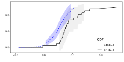
Figure 5: Estimated CDFs

It turns out that the estimated CDF for the treated outcome is well below that for the untreated outcome. Formally, I take all observed values of cumulative returns as the evaluation points, and then simulate the maximum of the approximation process by taking $500$ draws of random weights $\{\omega_{i}\}_{i=1}^{n}$. In this simple example, the test statistic equals $0$, which is well below the critical value $7.5$ for a confidence level of $0.95$ obtained through simulation. Thus, SD of $\theta_{1,1}(\cdot)$ over $\theta_{0,1}(\cdot)$ cannot be rejected. It implies that the positive effects of political connections in this example are felt over the entire distribution of the stock returns of financial firms connected with Geithner, which is a stronger conclusion than that based simply on the mean in Section 3.

5.2 High-Rank Covariates

The analysis so far is based on Equation (2.6), assuming $\bm{x}_{i}$ takes a purely nonlinear factor structure. However, high-rank components may exist in $\bm{x}_{i}$, and it is the latent structure of the residuals that contains relevant information on $\bm{\alpha}_{i}$, as described by Equation (2.5). It can be viewed as a generalization of linear regression with interactive fixed effects. Intuitively, due to the existence of the unknown $\eta_{t}(\bm{\alpha}_{i})$, the regressors $\bm{w}_{i,\ell}$ have to be sufficiently high-rank, otherwise they will be too collinear with the latent component and $\{\vartheta_{\ell}\}_{\ell=1}^{\mathsf{d}_{w}}$ cannot be identified. This is similar to the identification condition for semiparametric partially linear regression.

The main analysis of this paper can still be applied once we have some consistent estimators of $\vartheta_{\ell}$’s. They can be obtained using the idea of partially linear regression. Specifically, I refer to Step 1 in Section 3.1 as a general local principal subspace approximation procedure, which will be applied to other sequences in addition to $\{\bm{x}_{i}\}$. A slightly revised estimation procedure can be used to extract the latent variables:

1. Randomly split the row index set $\mathcal{T}=\{1,\cdots,T\}$ into three (non-overlapping) portions: $\mathcal{T}=\mathcal{T}_{1}\cup\mathcal{T}_{2}\cup\mathcal{T}_{3}$.

2. On $\mathcal{T}_{1}\cup\mathcal{T}_{2}$, for each $\ell=1,\ldots,\mathsf{d}_{w}$, apply local principal subspace approximation to $\{\bm{w}_{i,\ell}\}_{i=1}^{n}$. Obtain residuals $\widehat{\bm{e}}_{i,\ell}:=\bm{w}_{i,\ell}-\widehat{\bm{w}}_{i,\ell}$. Use $\mathcal{T}_{1}$ for $K$-NN matching and $\mathcal{T}_{2}$ for local PCA.

3. On $\mathcal{T}_{1}\cup\mathcal{T}_{2}$, apply the same procedure to $\{\bm{x}_{i}\}_{i=1}^{n}$. Let the obtained residuals be $\widehat{\bm{u}}^{\natural}_{i}=\bm{x}_{i}-\widehat{\bm{x}}_{i}$.

4. Let $\widehat{\bm{e}}_{i}=(\widehat{\bm{e}}_{i,1},\cdots,\widehat{\bm{e}}_{i,\mathsf{d}_{w}})^{\prime}$. Estimate $\bm{\vartheta}=(\vartheta_{1},\cdots,\vartheta_{\mathsf{d}_{w}})^{\prime}$ by

   $$\widehat{\bm{\vartheta}}=\Big{(}\frac{1}{n}\sum_{i=1}^{n}\widehat{\bm{e}}_{i}\widehat{\bm{e}}_{i}^{\prime}\Big{)}^{-1}\Big{(}\frac{1}{n}\sum_{i=1}^{n}\widehat{\bm{e}}_{i}\widehat{\bm{u}}^{\natural}_{i}\Big{)}.$$

5. On $\mathcal{T}_{2}\cup\mathcal{T}_{3}$, apply the local principal subspace approximation to the covariates-adjusted $\bm{x}_{i}$, i.e., $\{\bm{x}_{i}-\sum_{\ell=1}^{\mathsf{d}_{w}}\bm{w}_{i,\ell}\widehat{\vartheta}_{\ell}\}_{i=1}^{n}$. Use $\mathcal{T}_{2}$ for $K$-NN matching and $\mathcal{T}_{3}$ for local PCA. The index sets for nearest neighbors and factor loadings obtained from this step are denoted by $\{\mathcal{N}_{i}\}_{i=1}^{n}$ and $\{\widehat{\bm{\Lambda}}_{\langle i\rangle}\}_{i=1}^{n}$ respectively, which are the only quantities carried to counterfactual analysis.

Under additional regularity conditions on $\{\bm{w}_{i,\ell}\}_{\ell=1}^{\mathsf{d}_{w}}$, it can be shown that $\widehat{\bm{\vartheta}}$ converges to $\bm{\vartheta}$ sufficiently fast and the main results established previously still hold. Formal analysis is available in Section SA-6 of the SA and is omitted here to conserve space.

5.3 Generalized Partially Linear Forms

The analysis so far focuses on the simplified models (2.3) and (2.4). It can be extended to generalized partially linear models described by (2.1) and (2.2). We can employ the local quasi-maximum likelihood method. For Equation (2.1), consider a quasi-log-likelihood function $\mathcal{L}_{\mathsf{y}}(\varsigma,y)$ such that $\frac{\partial}{\partial\varsigma}\mathcal{L}_{\mathsf{y}}(\varsigma,y)=\frac{y-\varsigma}{V_{\mathsf{y}}(\varsigma)}$ for some positive function $V_{\mathsf{y}}$. An estimator of $\varsigma_{i,\jmath}$ is given by

$$\begin{split}&\widehat{\varsigma}_{i,\jmath}=\psi_{\mathsf{y}}(\bm{z}_{i}^{\prime}\widehat{\bm{\beta}}_{\jmath,\langle i\rangle}+\widehat{\mu}_{\jmath}(\bm{\alpha}_{i})),\quad\widehat{\mu}_{\jmath}(\bm{\alpha}_{i})=\widehat{\bm{\lambda}}_{i,\langle i\rangle}^{\prime}\widehat{\bm{b}}_{\jmath,\langle i\rangle},\quad\text{where}\\[10.00002pt] &(\widehat{\bm{\beta}}_{\jmath,\langle i\rangle}^{\prime},\,\widehat{\bm{b}}_{\jmath,\langle i\rangle}^{\prime})^{\prime}=\operatorname*{arg\,max}_{(\bm{\beta}^{\prime},\bm{b}^{\prime})^{\prime}\in\mathbb{R}^{\mathsf{d}_{z}+\mathsf{d}_{\lambda}}}\;\sum_{\ell\in\mathcal{N}_{i}}d_{\ell}(\jmath)\mathcal{L}_{\mathsf{y}}\Big{(}\psi_{\mathsf{y}}(\bm{z}_{\ell}^{\prime}\bm{\beta}+\widehat{\bm{\lambda}}_{\ell,\langle i\rangle}^{\prime}\bm{b}),\;y_{\ell}\Big{)}.\end{split}$$

For each $i$, the fitting is restricted to its local neighborhood $\mathcal{N}_{i}$. Equation (2.2) can be treated similarly by appropriately choosing a quasi-likelihood $\mathcal{L}_{\mathsf{s}}(\cdot,\cdot)$ associated with $\{V_{\mathsf{s},\jmath}(\cdot)\}_{\jmath\in\mathcal{J}}$ satisfying $\frac{\partial}{\partial\zeta_{\jmath}}\mathcal{L}_{\mathsf{s}}(\bm{\psi}_{\mathsf{s}}(\bm{\zeta}),\bm{d})=\frac{d(\jmath)-\psi_{\mathsf{s},\jmath}(\bm{\zeta})}{V_{\mathsf{s},\jmath}(\bm{\zeta})}$. The predicted conditional treatment probability is given by $\widehat{\bm{p}}_{i}=(\widehat{p}_{i,0},\cdots,\widehat{p}_{i,J})^{\prime}=\bm{\psi}_{\mathsf{s}}(\widehat{\bm{\gamma}}\bm{z}_{i}+\bm{\widehat{\rho}}(\bm{\alpha}_{i}))$. The asymptotic properties of these estimators can be derived under additional regularity conditions on the quasi-likelihood and link functions. See Section SA-6 of the SA for details.

Alternatively, one may exploit other standard methods in the semiparametrics literature, e.g., profiled quasi-maximum likelihood, to estimate the parametric components $\bm{\beta}_{\jmath}$’s and $\bm{\gamma}_{\jmath}$’s, though it is computationally more burdensome. See Härdle, Müller, Sperlich, and Werwatz (2004) for implementation details.

6 Conclusion

This paper has developed a causal inference method for treatment effects models with some confounders not directly observed. Relevant information on these latent confounders is extracted from a large set of noisy measurements that admits an unknown, possibly nonlinear factor structure. Such information is then used to match comparable units in the subsequent counterfactual analysis. Large-sample properties of the proposed estimators are established. The results cover a large class of causal parameters, including average treatment effects and counterfactual distributions. The method is illustrated with an empirical application studying the effect of political connections on stock returns of financial firms.

References

- (1)
- Abadie (2021) Abadie, A. (2021): “Using synthetic controls: Feasibility, data requirements, and methodological aspects,” Journal of Economic Literature, 59(2), 391–425.
- Abadie and Cattaneo (2018) Abadie, A., and M. D. Cattaneo (2018): “Econometric Methods for Program Evaluation,” Annual Review of Economics, 10, 465–503.
- Abadie and Imbens (2006) Abadie, A., and G. W. Imbens (2006): “Large Sample Properties of Matching Estimators for Average Treatment Effects,” Econometrica, 74(1), 235–267.
- Abadie and L’Hour (2021) Abadie, A., and J. L’Hour (2021): “A Penalized Synthetic Control Estimator for Disaggregated Data,” Journal of the American Statistical Association, forthcoming.
- Abbe, Fan, Wang, Zhong, et al. (2020) Abbe, E., J. Fan, K. Wang, Y. Zhong, et al. (2020): “Entrywise Eigenvector Analysis of Random Matrices with Low Expected Rank,” Annals of Statistics, 48(3), 1452–1474.
- Acemoglu, Johnson, Kermani, Kwak, and Mitton (2016) Acemoglu, D., S. Johnson, A. Kermani, J. Kwak, and T. Mitton (2016): “The Value of Connections in Turbulent Times: Evidence from the United States,” Journal of Financial Economics, 121(2), 368–391.
- Ahn and Horenstein (2013) Ahn, S. C., and A. R. Horenstein (2013): “Eigenvalue Ratio Test for the Number of Factors,” Econometrica, 81(3), 1203–1227.
- Altonji and Mansfield (2018) Altonji, J. G., and R. K. Mansfield (2018): “Estimating Group Effects Using Averages of Observables to Control for Sorting on Unobservables: School and Neighborhood Effects,” American Economic Review, 108(10), 2902–46.
- Angrist and Pischke (2008) Angrist, J. D., and J.-S. Pischke (2008): Mostly Harmless Econometrics: An Empiricist’s Companion. Princeton University Press, Princeton.
- Arellano (2003) Arellano, M. (2003): Panel Data Econometrics. Oxford University Press, Oxford.
- Arias-Castro, Lerman, and Zhang (2017) Arias-Castro, E., G. Lerman, and T. Zhang (2017): “Spectral Clustering Based on Local PCA,” Journal of Machine Learning Research, 18(1), 253–309.
- Athey and Imbens (2021) Athey, S., and G. W. Imbens (2021): “Design-based Analysis in Difference-in-Differences Settings with Staggered Adoption,” Journal of Econometrics, forthcoming.
- Bai (2003) Bai, J. (2003): “Inferential Theory for Factor Models of Large Dimensions,” Econometrica, 71(1), 135–171.
- Bai (2009) (2009): “Panel Data Models with Interactive Fixed Effects,” Econometrica, 77(4), 1229–1279.
- Bai and Ng (2002) Bai, J., and S. Ng (2002): “Determining the Number of Factors in Approximate Factor Models,” Econometrica, 70(1), 191–221.
- Bai and Ng (2006) (2006): “Confidence Intervals for Diffusion Index Forecasts and Inference for Factor-Augmented Regressions,” Econometrica, 74(4), 1133–1150.
- Bai and Wang (2016) Bai, J., and P. Wang (2016): “Econometric Analysis of Large Factor Models,” Annual Review of Economics, 8, 53–80.
- Barrett and Donald (2003) Barrett, G. F., and S. G. Donald (2003): “Consistent Tests for Stochastic Dominance,” Econometrica, 71(1), 71–104.
- Belloni, Chernozhukov, and Hansen (2014) Belloni, A., V. Chernozhukov, and C. Hansen (2014): “Inference on Treatment Effects after Selection among High-Dimensional Controls,” The Review of Economic Studies, 81(2), 608–650.
- Bishop (2006) Bishop, C. M. (2006): “Continuous Latent Variables,” in Pattern Recognition and Machine Learning, chap. 12, pp. 559–604. Springer, New York.
- Bonhomme, Lamadon, and Manresa (2021) Bonhomme, S., T. Lamadon, and E. Manresa (2021): “Discretizing Unobserved Heterogeneity,” Econometrica, forthcoming.
- Cattaneo (2010) Cattaneo, M. D. (2010): “Efficient Semiparametric Estimation of Multi-valued Treatment Effects under Ignorability,” Journal of Econometrics, 155(2), 138–154.
- Cattaneo and Jansson (2018) Cattaneo, M. D., and M. Jansson (2018): “Kernel-Based Semiparametric Estimators: Small Bandwidth Asymptotics and Bootstrap Consistency,” Econometrica, 86(3), 955–995.
- Cattaneo, Jansson, and Ma (2019) Cattaneo, M. D., M. Jansson, and X. Ma (2019): “Two-Step Estimation and Inference with Possibly Many Included Covariates,” The Review of Economic Studies, 86(3), 1095–1122.
- Chernozhukov, Chetverikov, Demirer, Duflo, Hansen, Newey, and Robins (2018) Chernozhukov, V., D. Chetverikov, M. Demirer, E. Duflo, C. Hansen, W. Newey, and J. Robins (2018): “Double/Debiased Machine Learning for Treatment and Structural Parameters,” The Econometrics Journal, 21(1), C1–C68.
- Chernozhukov, Escanciano, Ichimura, Newey, and Robins (2020) Chernozhukov, V., J. C. Escanciano, H. Ichimura, W. K. Newey, and J. M. Robins (2020): “Locally Robust Semiparametric Estimation,” arXiv preprint arXiv:1608.00033.
- Chernozhukov, Fernández-Val, and Melly (2013) Chernozhukov, V., I. Fernández-Val, and B. Melly (2013): “Inference on Counterfactual Distributions,” Econometrica, 81(6), 2205–2268.
- Chernozhukov and Hansen (2005) Chernozhukov, V., and C. Hansen (2005): “An IV Model of Quantile Treatment Effects,” Econometrica, 73(1), 245–261.
- Chernozhukov, Hansen, Liao, and Zhu (2020) Chernozhukov, V., C. Hansen, Y. Liao, and Y. Zhu (2020): “Inference for Heterogeneous Effects using Low-Rank Estimation of Factor Slopes,” arXiv preprint arXiv:1812.08089.
- Cunha, Heckman, and Schennach (2010) Cunha, F., J. J. Heckman, and S. M. Schennach (2010): “Estimating the Technology of Cognitive and Noncognitive Skill Formation,” Econometrica, 78(3), 883–931.
- Donald and Hsu (2014) Donald, S. G., and Y.-C. Hsu (2014): “Estimation and Inference for Distribution Functions and Quantile Functions in Treatment Effect Models,” Journal of Econometrics, 178, 383–397.
- Fan and Gijbels (1996) Fan, J., and I. Gijbels (1996): Local Polynomial Modelling and Its Applications. Chapman & Hall, London.
- Farrell (2015) Farrell, M. H. (2015): “Robust Inference on Average Treatment Effects with Possibly More Covariates than Observations,” Journal of Econometrics, 189(1), 1–23.
- Györfi, Kohler, Krzyzak, and Walk (2002) Györfi, L., M. Kohler, A. Krzyzak, and H. Walk (2002): “k-NN Estimates,” in A Distribution-Free Theory of Nonparametric Regression, chap. 6, pp. 86–99. Springer, New York.
- Härdle, Müller, Sperlich, and Werwatz (2004) Härdle, W. K., M. Müller, S. Sperlich, and A. Werwatz (2004): Nonparametric and Semiparametric Models. Springer, Berlin.
- Heckman and Vytlacil (2007) Heckman, J. J., and E. J. Vytlacil (2007): “Econometric Evaluation of Social Programs, Part I: Causal Models, Structural Models and Econometric Policy Evaluation,” in Handbook of Econometrics, ed. by J. J. Heckman, and E. E. Leamer, vol. 6, chap. 70, pp. 4779–4874. Elsevier, Amsterdam.
- Hernán and Robins (2020) Hernán, M. A., and J. M. Robins (2020): Causal Inference: What If. Chapman & Hall/CRC, Boca Raton.
- Hu and Schennach (2008) Hu, Y., and S. M. Schennach (2008): “Instrumental Variable Treatment of Nonclassical Measurement Error Models,” Econometrica, 76(1), 195–216.
- Imbens and Rubin (2015) Imbens, G. W., and D. B. Rubin (2015): Causal Inference in Statistics, Social, and Biomedical sciences. Cambridge University Press, Cambridge.
- Matsushita and Otsu (2021) Matsushita, Y., and T. Otsu (2021): “Jackknife Empirical Likelihood: Small Bandwidth, Sparse Network and High-dimensional Asymptotics,” Biometrika, 108(3), 661–674.
- Newey and Powell (2003) Newey, W. K., and J. L. Powell (2003): “Instrumental Variable Estimation of Nonparametric Models,” Econometrica, 71(5), 1565–1578.
- Peng, Lu, and Wang (2015) Peng, Y., B.-L. Lu, and S. Wang (2015): “Enhanced Low-Rank Representation via Sparse Manifold Adaption for Semi-Supervised Learning,” Neural Networks, 65, 1–17.
- Robins and Rotnitzky (1995) Robins, J. M., and A. Rotnitzky (1995): “Semiparametric Efficiency in Multivariate Regression Models with Missing Data,” Journal of the American Statistical Association, 90(429), 122–129.
- Roweis and Saul (2000) Roweis, S. T., and L. K. Saul (2000): “Nonlinear Dimensionality Reduction by Locally Linear Embedding,” Science, 290(5500), 2323–2326.
- Schennach (2016) Schennach, S. M. (2016): “Recent Advances in the Measurement Error Literature,” Annual Review of Economics, 8, 341–377.
- Stock and Watson (2002) Stock, J. H., and M. W. Watson (2002): “Forecasting Using Principal Components from a Large Number of Predictors,” Journal of the American Statistical Association, 97(460), 1167–1179.
- Van Der Vaart and Wellner (1996) Van Der Vaart, A. W., and J. A. Wellner (1996): Weak Convergence and Empirical Processes, Springer Series in Statistics. Springer, New York.
- Wang and Fan (2017) Wang, W., and J. Fan (2017): “Asymptotics of Empirical Eigenstructure for High Dimensional Spiked Covariance,” Annals of Statistics, 45(3), 1342.
- Wooldridge (2015) Wooldridge, J. M. (2015): “Control Function Methods in Applied Econometrics,” Journal of Human Resources, 50(2), 420–445.
- Yalcin and Amemiya (2001) Yalcin, I., and Y. Amemiya (2001): “Nonlinear Factor Analysis as a Statistical Method,” Statistical Science, pp. 275–294.
- Zhang, Zhang, Zhang, Tao, Huang, and Du (2015) Zhang, L., Q. Zhang, L. Zhang, D. Tao, X. Huang, and B. Du (2015): “Ensemble Manifold Regularized Sparse Low-Rank Approximation for Multiview Feature Embedding,” Pattern Recognition, 48(10), 3102–3112.
- Zhang, Levina, and Zhu (2017) Zhang, Y., E. Levina, and J. Zhu (2017): “Estimating Network Edge Probabilities by Neighbourhood Smoothing,” Biometrika, 104(4), 771–783.
- Zhang and Zha (2004) Zhang, Z., and H. Zha (2004): “Principal Manifolds and Nonlinear Dimensionality Reduction via Tangent Space Alignment,” SIAM Journal on Scientific Computing, 26(1), 313–338.