Single-ion anisotropy effects on the critical behaviors of quantum entanglement and correlation in the spin-1 Heisenberg chain

Abstract

Quantum entanglement and correlations in the spin-1 Heisenberg chain with single-ion anisotropy are investigated using the quantum renormalization group method. Negativity and quantum discord (QD) are calculated with various anisotropy parameters $\bigtriangleup$ and single-ion anisotropy parameters $D$. We focus on the relations between two abovementioned physical quantities and on transitions between the Néel, Haldane, and Large-D phases. It is found that both negativity and QD exhibit step-like patterns in different phases as the size of the system increases. Interestingly, the single-ion anisotropy parameter $D$, which can be modulated using nuclear electric resonance (2020 Nature 579 205), plays an important role in tuning the quantum phase transition (QPT) of the system. Both the first partial derivative of the negativity and quantum discord with respect to $D$ or $\bigtriangleup$ exhibit nonanalytic behavior at the phase transition points, which corresponds directly to the divergence of the correlation length. The quantum correlation critical exponents derived from negativity and QD are equal, and are the reciprocal of the correlation length exponent at each critical point. This work extends the application of quantum entanglement and correlations as tools for depicting QPTs in spin-1 systems.

I Introduction

Entanglement is a peculiar correlation in quantum systems, which is the fundamental difference between quantum and classical physics Bennett et al. (1993). In the past two decades, quantum entanglement has attracted much attention due to its novel physical properties and its potential applications in the development of quantum computers and quantum information devices Zheng and Guo (2000). It has been realized as a crucial resource in processing and sending quantum information Ekert (1991); Bouwmeester et al. (1997). Recently, it has been found that quantum entanglement has a close relationship with quantum phase transitions (QPTs) and can be widely exploited for indicating QPTs Hill and Wootters (1997); Osterloh et al. (2002); Vidal et al. (2003); Verstraete et al. (2004). Besides quantum entanglement, quantum discord (QD) gives a more common conception of quantum correlations (QCs), which even occurs in unentangled systems, and is also a useful measurement tool for depicting QPTs Ollivier and Zurek (2001); Chen et al. (2011). QPTs occur at absolute zero temperature, which is induced by the change of an external parameter or coupling constant. In condensed matter physics, this mechanism is at the core of relevant quantum phenomena such as superconductivity and the quantum Hall effect Sachdev (2007). Research into QPTs is also one of the most interesting topics in strongly correlated systems, to emerge during the last decade, and investigations of the relation between QCs and QPTs has attracted much attention recently Osterloh et al. (2002); Osborne and Nielsen (2002); Sachdev (2007).

In the field of strongly correlated systems, various methods are used extensively to investigate the properties of many-body systems, such as the renormalization group method Wilson (1975); Burkhardt and van Leeuwen (2012), the density matrix renormalization group method White (1992); Xiang (1996); Tzeng and Yang (2008); Gong et al. (2015); Zhang et al. (2017), and the tensor renormalization group approach Verstraete and Cirac (2004); Li et al. (2011, 2019). In addition, the quantum renormalization group (QRG) is also a popular analytic method for investigating the behavior of quantum spin systems. Quantum entanglement in one- and two-dimensional spin systems has been investigated using the QRG method, which exhibits nonanalytic and scaling behaviors in the vicinity of the quantum critical points Langari (2004); Kargarian et al. (2008); Jafari et al. (2008); Xu et al. (2014, 2016); Farajollahpour and Jafari (2018). In particular, quantum entanglement in, and QPTs of, spin-1/2 XY models, including ones with staggered Dzyaloshinskii-Moriya interactions, were studied using the QRG method. In these cases, the behavior of the entanglement is closely associated with the quantum critical properties, and the relation between the entanglement exponent and the correlation length exponent was obtained in Ma et al. (2011a, b). Furthermore, the critical properties of spin systems on a fractal lattice can also be depicted using entanglement, based on the QRG method Xu et al. (2017); Cheng and Xu (2018).

The low-energy behavior of spin-1/2 systems, such as the XY, XYZ, and XXZ models were extensively investigated in Langari (2004); Kargarian et al. (2008); Ma et al. (2011a), whereas QCs in higher spin systems have been less studied until now. Furthermore, the spin profile of many organic Ni materials with significant single-ion anisotropy can be described by the spin-1 Heisenberg chain Regnault et al. (1994); Zheludev et al. (1996), and single-ion anisotropy interactions can be precisely manipulated using the latest experimental techniques, such as Nuclear Electric Resonance Asaad et al. (2020). It is important to investigate the spin-1 Heisenberg chain with a single-ion anisotropy in the field of condensed matter and quantum information Tzeng and Yang (2008); Schulz (1986); Chen et al. (2003); Hu et al. (2011); Ren et al. (2018). In previous work, the QRG-flow equations and phase diagram of the spin-1 Heisenberg chain were obtained using the QRG method Langari et al. (2013). The dynamical spin excitations of this model were also investigated using quantum Monte Carlo simulations and stochastic analytic continuation Huang et al. (2021). To the best of the authors’ knowledge, the effects of single-ion anisotropy on the critical behavior of quantum entanglement and correlations in the spin-1 Heisenberg chain have been investigated systematically except in the present work.

In this work, the QCs and QPTs of the spin-1 Heisenberg chain with single-ion anisotropy are investigated using the QRG method. Both the calculated negativity and QD are affected by the easy-axis anisotropy and the single-ion anisotropy parameters. The single-ion anisotropy can effect the negativity and QD by favoring the alignment of spins. For the given values of the anisotropy or single-ion anisotropy parameters, both negativity and QD exhibit step-like patterns in different phases, which are separated by the phase transition points as the size of the system increases. Furthermore, the first partial derivative of the negativity and the QD with respect to the anisotropy or single-ion anisotropy parameters show nonanalytic behavior with a scaling relation at the phase transition points. Besides, it is found that negativity and QD depict the QPT in slightly different ways. This paper is organized as follows. In Sec. II, the spin model and the QRG method are introduced. In Sec. III, the entanglement and QD between two blocks are investigated. We discuss the nonanalytic and the scaling behaviors of the entanglement and QD in Sec. IV, and summarize in Sec. V.

II Model and quantum renormalization group method

The Hamiltonian of the spin-1 Heisenberg chain with a single-ion anisotropy is given by

$$H=J\sum_{i=1}^{L}[S_{i}^{x}S_{i+1}^{x}+S_{i}^{y}S_{i+1}^{y}+\bigtriangleup S_{i}^{z}S_{i+1}^{z}+D(S_{i}^{z})^{2}],$$ (1)

where $S^{\alpha}(\alpha=x,y,z)$ are spin-1 operators, $J>0$ is the antiferromagnetic nearest-neighbor interaction, and $\bigtriangleup$ characterizes the easy-axis anisotropy. The single-ion anisotropy parameter $D$ can be adjusted in an experiment by utilising the latest developments in nuclear electric resonance Asaad et al. (2020). The phase diagram of Hamiltonian Eq.(1) is well established Schulz (1986); Chen et al. (2003); Hu et al. (2011). Here, we focus our attention on phase transitions among the Néel, Haldane, and large-D phases for $\bigtriangleup\geq 0$. Most parts of the phase diagram are determined accurately. However, it is difficult to accurately determine the tri-critical point using numerical analysis.

The quantum fidelity and QPT of the model were investigated using the QRG method, based on Kadanoff’s block approach Langari et al. (2013). The general idea of the QRG method is to keep the most important degrees of freedom and integrate out the rest by an iterative procedure. In this work, the three sites (marked as 1-2-3) of the spin chain are considered as a block, as shown in figure 1, which maps the initial Hamiltonian into a renormalized Hamiltonian defined by the set of renormalized couplings $\left(J^{{}^{\prime}},\bigtriangleup^{{}^{\prime}},D^{{}^{\prime}}\right)$. The relations between the original and renormalized coupling constants are

$$J^{{}^{\prime}}=\left(X_{ren}\right)^{2}J,$$ (2)

$$\bigtriangleup^{{}^{\prime}}=\left(\frac{Z_{ren}}{X_{ren}}\right)^{2}\bigtriangleup,$$ (3)

$$D^{{}^{\prime}}=\frac{E_{1}-E_{0}}{\left(X_{ren}\right)^{2}},$$ (4)

where $X_{ren}$ and $Z_{ren}$ are the renormalization coefficients, $E_{0}$ is the ground-state energy of the block Hamiltonian and $E_{1}$ is the first excited-state energy. The first excited-state energy is doubly degenerate. The explicit form of the renormalized couplings and the details of the renormalization procedure are presented in the appendix A. The renormalization of the couplings generates the flow of the couplings, which in turn determines the quantum phase diagram and the ground-state properties of the model. The analysis of the QRG-flow Eqs.(2)(3)(4) gives a clear picture of the topography in the ground-state phase diagram. A sketch of the phase diagram is given in figure 2. The QRG-flow includes two types of fixed points $(\bigtriangleup,D)$, $P_{1}:(1.0,0)$, $P_{2}:(0,0.58)$, $P_{3}:(0,1.45)$, $P_{4}:(0,-1.91)$, and $P_{5}:(3.0,2.27)$ are fixed points and two others are for extremely large couplings, namely $\left(\infty,0\right)$ and $\left(-\infty,\infty\right)$. In particular, both $P_{3}:(0,1.45)$ and $P_{4}:(0,-1.91)$ are quantum critical points, while $P_{5}:(3.0,2.27)$ is the tri-critical point Langari et al. (2013).

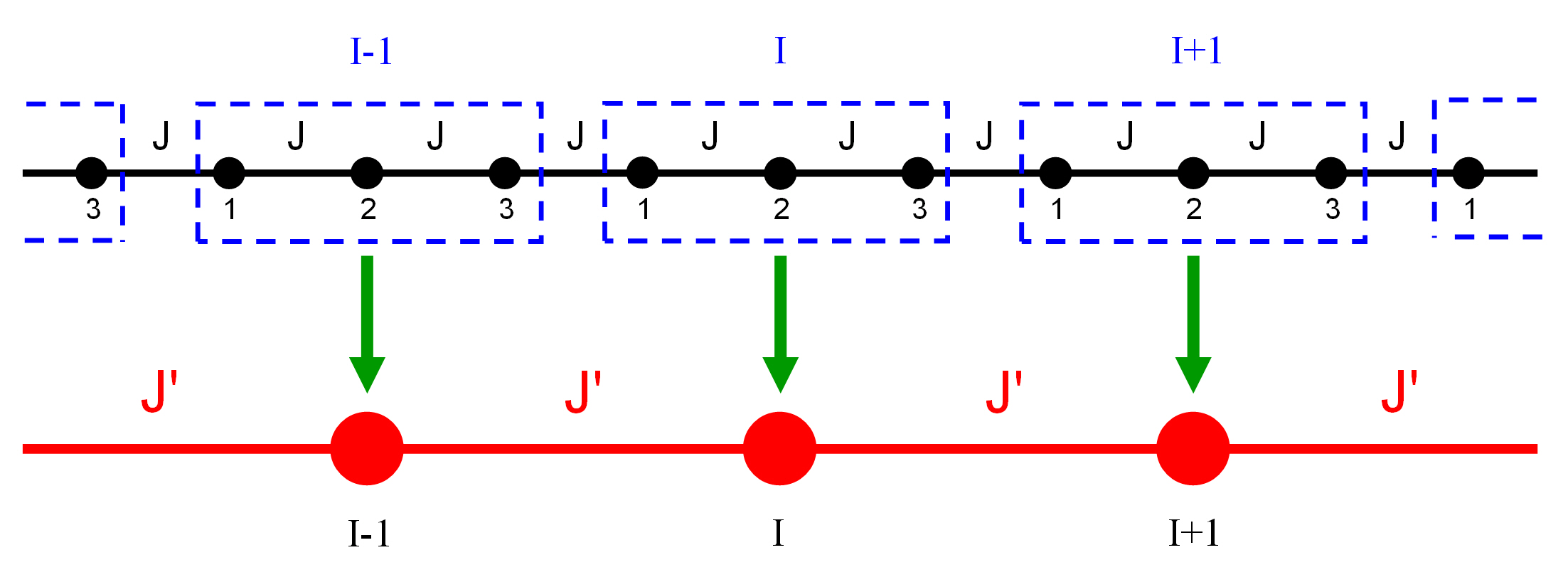
Figure 1: Sketch of the renormalization process for the spin-1 chain. The black (red) dots represent the initial (effective) spins, and the dashed blue rectangles represent blocks of three spins Langari et al. (2013).

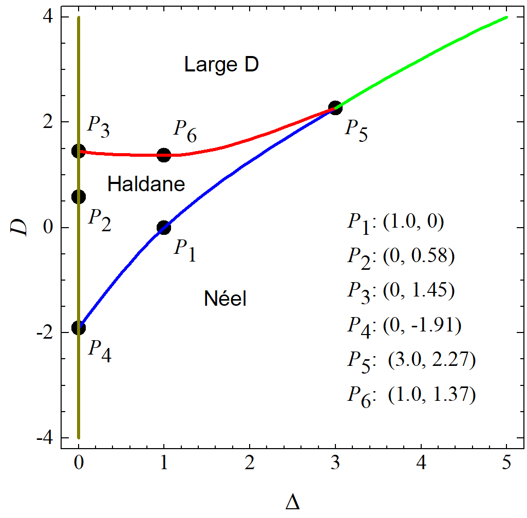
Figure 2: Sketch of the phase diagram for the spin-1 Heisenberg model with single-ion anisotropy. The color lines denote the boundaries between different phases, and the black dots represent the phase transition points $P_{1}$-$P_{6}$ Langari et al. (2013).

III Negativity and QD analysis

There are many measures for the pairwise entanglement and QC Hill and Wootters (1997); Wootters (1998); Vidal and Werner (2002); Chen et al. (2011). Here, we investigate the ground-state entanglement and QC between two blocks of the spin-1 Heisenberg chain using the measures of negativity and QD, and demonstrate how they vary as the size of the blocks increase. Consider the ground state $\left|\phi_{0}\right\rangle$ of a block and define the pure-state density matrix

$$\rho=\left|\phi_{0}\right\rangle\left\langle\phi_{0}\right|.$$ (5)

Because negativity measures the pairwise entanglement, the degrees of freedom for one site in the block should be traced out. Generally, the degrees of freedom of site 2 are traced so that the reduced density matrix for sites 1 and 3, i.e., $\rho_{13}$, can be obtained. The negativity of the partial transpose gives a sufficient condition for the entanglement of spin-1 particles. The negativity of sites 1 and 3 is defined as Vidal and Werner (2002)

$$N_{13}=\sum_{i}\left|\mu_{i}\right|,$$ (6)

where $\mu_{i}$ is the negative eigenvalue of $\rho_{13}^{T_{3}}$, and $T_{3}$ denotes the partial transpose with respect to the third spin. The value of $N_{13}$ varies in the range from $0$ to $1$. If $N_{13}=0$ or $1$, the system is unentangled or entangled maximally, respectively. Other values correspond to a partially entangled state Miranowicz and Grudka (2004).

QD can be applied to quantify QCs of the system, and is defined by the formula for mutual information. The quantum mutual information (QMI) of a bipartite quantum state $\rho_{AB}$ is Groisman et al. (2005)

$$I(\rho_{AB})=S(\rho_{A})+S(\rho_{B})-S(\rho_{AB}),$$ (7)

where $S\left(\rho\right)=-Tr\rho Log\rho$ is the von Neumann entropy of the state $\rho$. The classical correlation is defined in an alternative version of the mutual information as Malvezzi et al. (2016)

$$J(\rho_{AB})=S(\rho_{A})-min_{\left\{E_{k}^{B}\right\}}\sum_{k}p_{k}S(\rho_{A}|k),$$ (8)

where the minimum is taken over all possible positive operator-valued measures (POVMs) $\left\{E_{k}^{B}\right\}$ on subsystem B with $p_{k}=Tr\left(E_{k}^{B}\rho_{AB}\right)$ and $\rho_{A}|k=Tr_{B}\left(E_{k}^{B}\rho_{AB}\right)/p_{k}$. The functions $I(\rho_{AB})$ and $J(\rho_{AB})$ quantify the total correlation and classical correlation, respectively, and the QD measures the difference between the two Ollivier and Zurek (2001):

$$QD(\rho_{AB})=I(\rho_{AB})-J(\rho_{AB}).$$ (9)

QD is considered an effective measure of the QCs of a system, and we elaborate this numerically in the present work, using the random unitary matrix method. This allows us to find the minimum over all POVMs efficiently Chen et al. (2011); Malvezzi et al. (2016); Ollivier and Zurek (2001). As in the negativity defined above, the subscripts $A$ and $B$ in Eqs.(7)(8)(9) indicate the sites 1 and 3 in the spin block, respectively.

The numerical calculations indicate that both the negativity and the QD are influenced by the anisotropy parameter $\bigtriangleup$ and the single-ion anisotropy parameter $D$. For the three-site model, we plot the negativity $N_{13}$ versus $D$ for different values of $\bigtriangleup$, as shown in figure 3(a). The negativity is a decreasing function of the single-ion anisotropy $D$, regardless of the value of $\bigtriangleup$. In other words, the single-ion anisotropy suppresses the entanglement by favoring of the alignment of spins. As the single-ion anisotropy $D$ increases, the probability of the spin in the block tending to the direction of $\left|0\right\rangle$ is increased. In the limit $D\rightarrow\infty$, the system turns into a separable state, $\left|000\right\rangle$. Furthermore, when $D$ is small, $\bigtriangleup$ enhances the entanglement of the system when $\bigtriangleup\gg 0$, while it suppresses the entanglement as $D$ increases. The QD of the three-site model $QD_{13}$ has a similar tendency, as shown in figure 3(b). The quantum mutual information of the three-site model $QMI_{13}$ also has a similar tendency, as shown in figure S1(a) of appendix B. The curves of both $QD_{13}$ and $QMI_{13}$ are smoother than the curve of $N_{13}$.

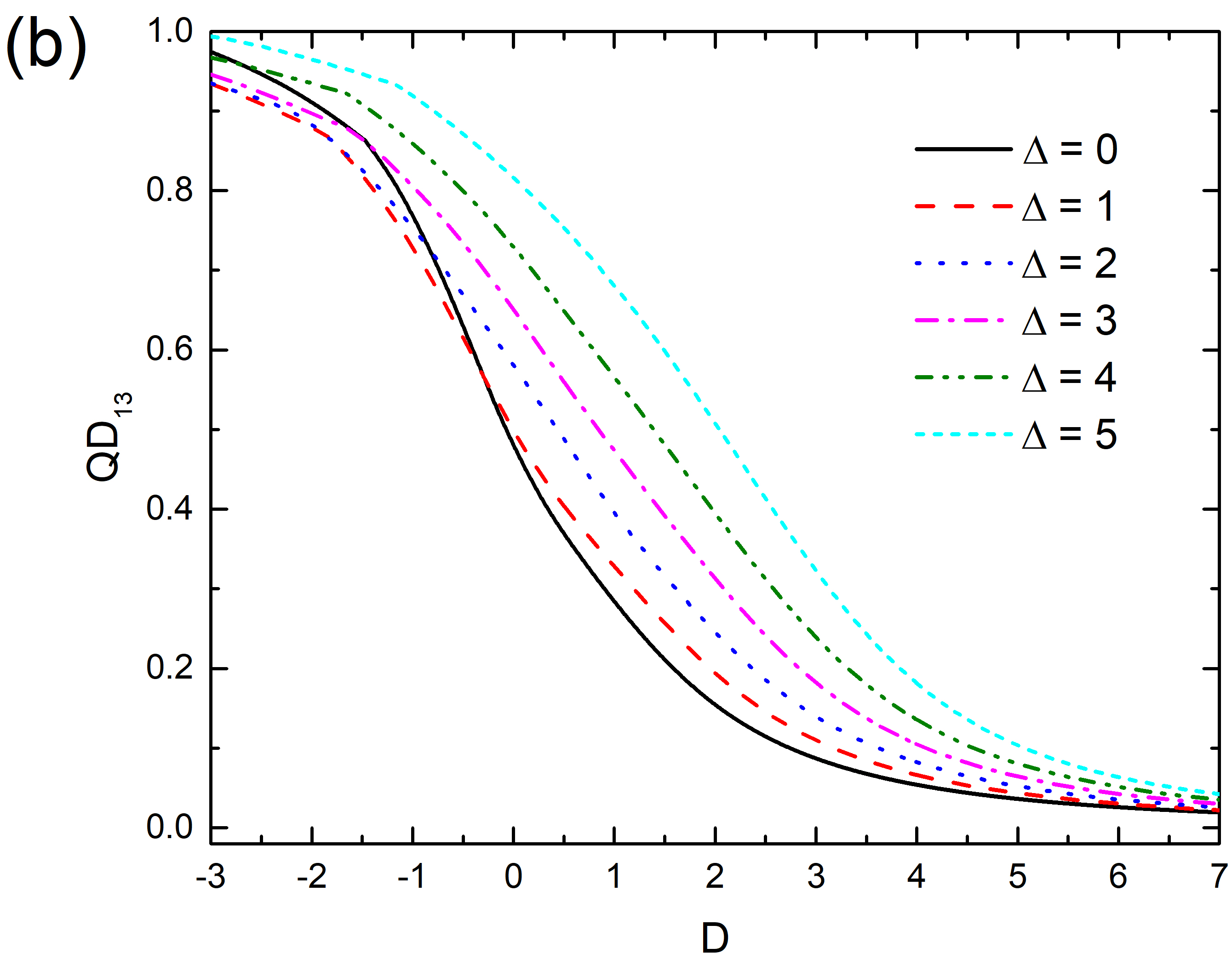
Figure 3: (a) Negativity and (b) QD between the first and third sites of the three-site model in terms of the single-ion anisotropy $D$ for different values of easy-axis anisotropy $\Delta$.

By combining the negativity with the QRG relations of the renormalized coupling constants, the entanglement for the large-sized system is calculated. A plot of the negativity ($N$) versus $D$, with fixed $\bigtriangleup=0$, is given in figure 4(a). The curves of negativity versus different steps of QRG cross each other at the fixed points. As the scale of the system increases, the negativity exhibits three step-like patterns in different phases separated by the phase transition points, as shown in the dashed green lines of the figure. The system driven by the single-ion anisotropy $D$ undergoes a transition from the Néel phase to the Haldane phase with an Ising transition at the critical point $P_{4}:(0,-1.91)$ Huang and Lin (2010). This turns the largest negativity into a smaller saturated value, which then vanishes in the large-D phase through a Gaussian transition at $P_{3}:(0,1.45)$. Previous works have shown that the Gaussian transition between the Haldane phase and large-D phase is a symmetry-protected topological phase transition. There is a lack of a local order parameter, and the critical exponents of the Gaussian transitions change continuously along the critical lines Schulz (1986); Tzeng and Yang (2008); Hu et al. (2011). At these fixed points, the system exhibits QCs because the negativity is a nonzero constant. The evolution of QD versus $D$ with $\bigtriangleup=0$ exhibits similar behavior, as shown in figure 4(b), as does the evolution of quantum mutual information ($QMI$) versus $D$ with $\bigtriangleup=0$ as shown in figure S1(b) of appendix B. This shows that quantum mutual information can also be used to depict the QPTs. All curves of negativity, QD, and quantum mutual information plotted against different steps of the QRG cross each other at the fixed points $P_{2}:(0,0.58)$. Amazingly, the QD curves present light humps at the critical point $P_{4}:(0,-1.91)$ as the size of the system increases, which differs from the behavior of negativity and quantum mutual information. For a fixed value of $\bigtriangleup=1$, the curves of negativity versus different steps of the QRG also cross each other at the fixed points and present step-like patterns in different phases separated by the fixed points as the system increases, as shown in figure 5(a). The system undergoes an Ising transition from the Néel phase to the Haldane phase at the fixed point $P_{1}:(1.0,0)$, which leads to the negativity becoming much smaller. Due to the alignment of spins, the negativity vanishes altogether in the large-D phase through a Gaussian transition at $P_{6}:(1.0,1.37)$. These negativities change smoothly as the single-ion anisotropy $D$ varies at the Gaussian transition points within SIX steps of RG iteration. The evolution of QD for $\bigtriangleup=1$ exhibits similar behavior, as shown in figure 5(b). Interestingly, both negativity and QD only develop two step-like patterns for $\bigtriangleup=3$, as shown in figures 6(a) and (b). With increasing $D$, the system undergoes QPTs from the Néel phase to the Haldane phase and to the large-D phase at $P_{5}:(3.0,2.27)$ Huang and Lin (2010). The values of negativity and QD can express the entanglement and correlation strength of the tri-critical point $P_{5}:(3.0,2.27)$, respectively. It is obvious that the system exhibits the same entanglement (or QC) at the tri-critical point as the size of the system increases, which is caused by the divergence of correlation length.

To compare the two, the negativity and QD are also analyzed by tuning $\bigtriangleup$ but fixing $D=0$. As the scale of the system increases, both the negativity and QD develop two step-like patterns separated by $P_{1}:(1.0,0)$, as shown in figure S2(a) and (b) of appendix B, respectively. In the thermodynamic limit, both negativity and QD jump to larger stable values as the system transforms from the Haldane phase to the Néel phase. The three-site model can describe the infinite spin-1 chain with renormalized coupling constants. At these critical points, quantum fluctuations play an important role and destroy any long-range order of the system. The negativity and QD show a clear drop at the Néel–Haldane and Néel–large-D phase transition points as the system reaches $3^{3}$ sites.

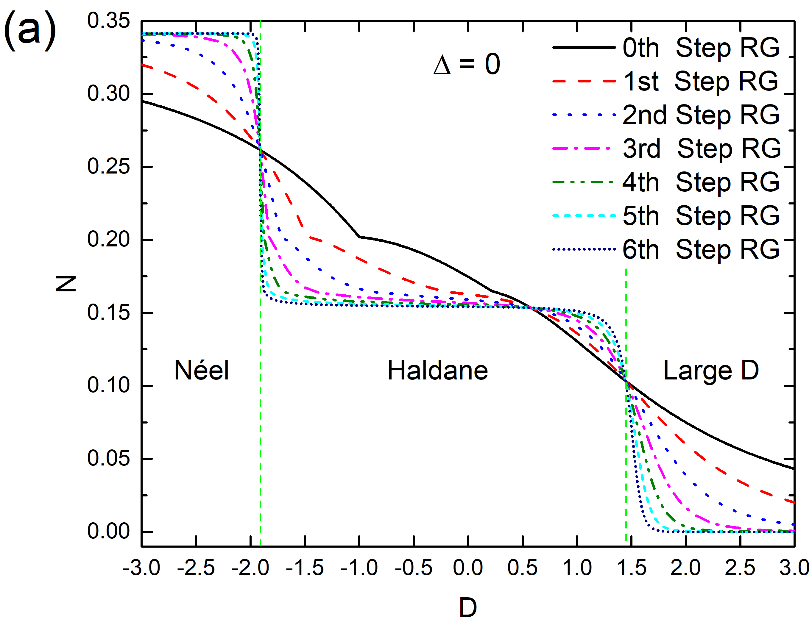
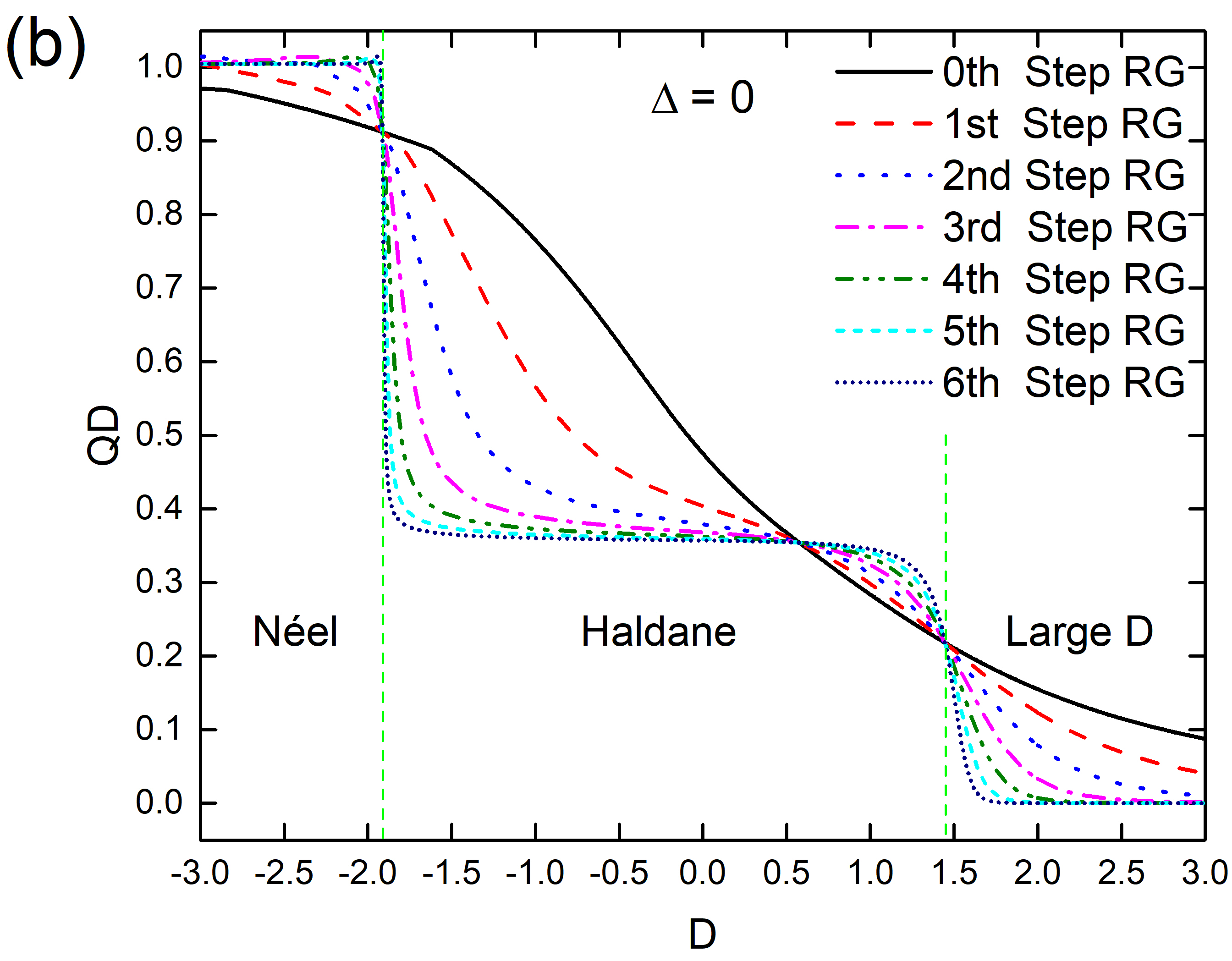
Figure 4: (a) Negativity and (b) QD in terms of QRG iterations at $\Delta=0$. Each phase is labelled by the black text, and separated by the dashed green lines at $D=-1.91$ and $D=1.45$, respectively.

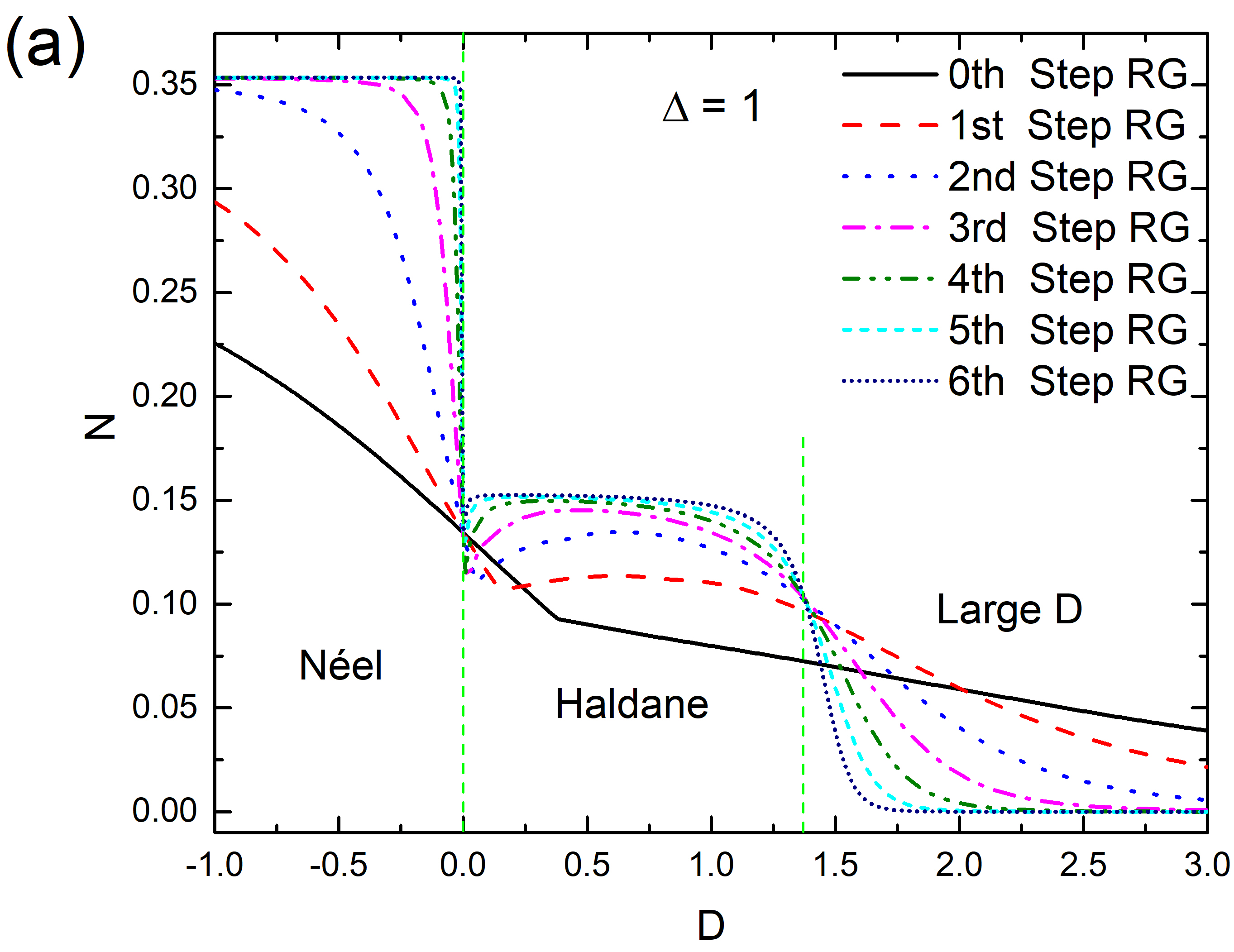
Figure 5: (a) Negativity and (b) QD in terms of QRG iterations at $\Delta=1$. Each phase is labelled by the black text, and separated by the dashed green lines at $D=0$ and $D=1.37$, respectively.

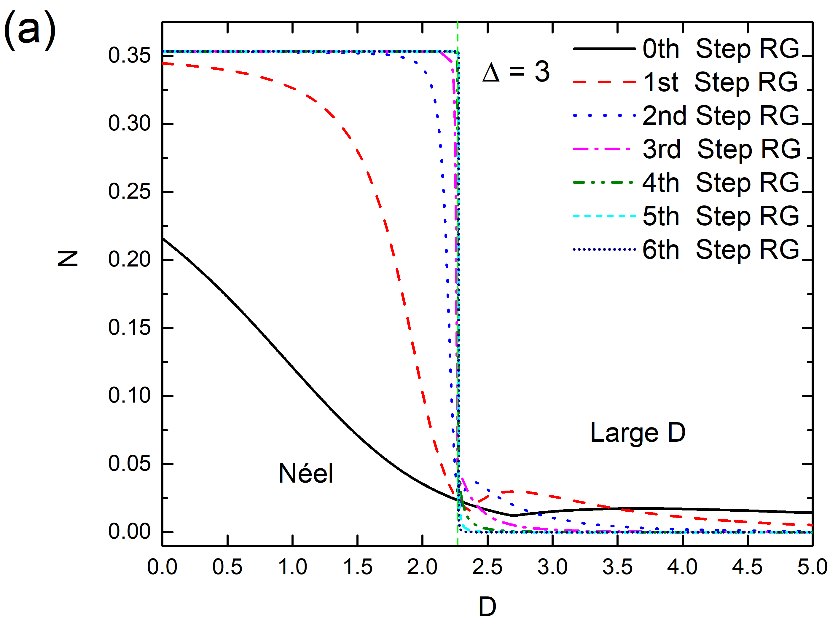
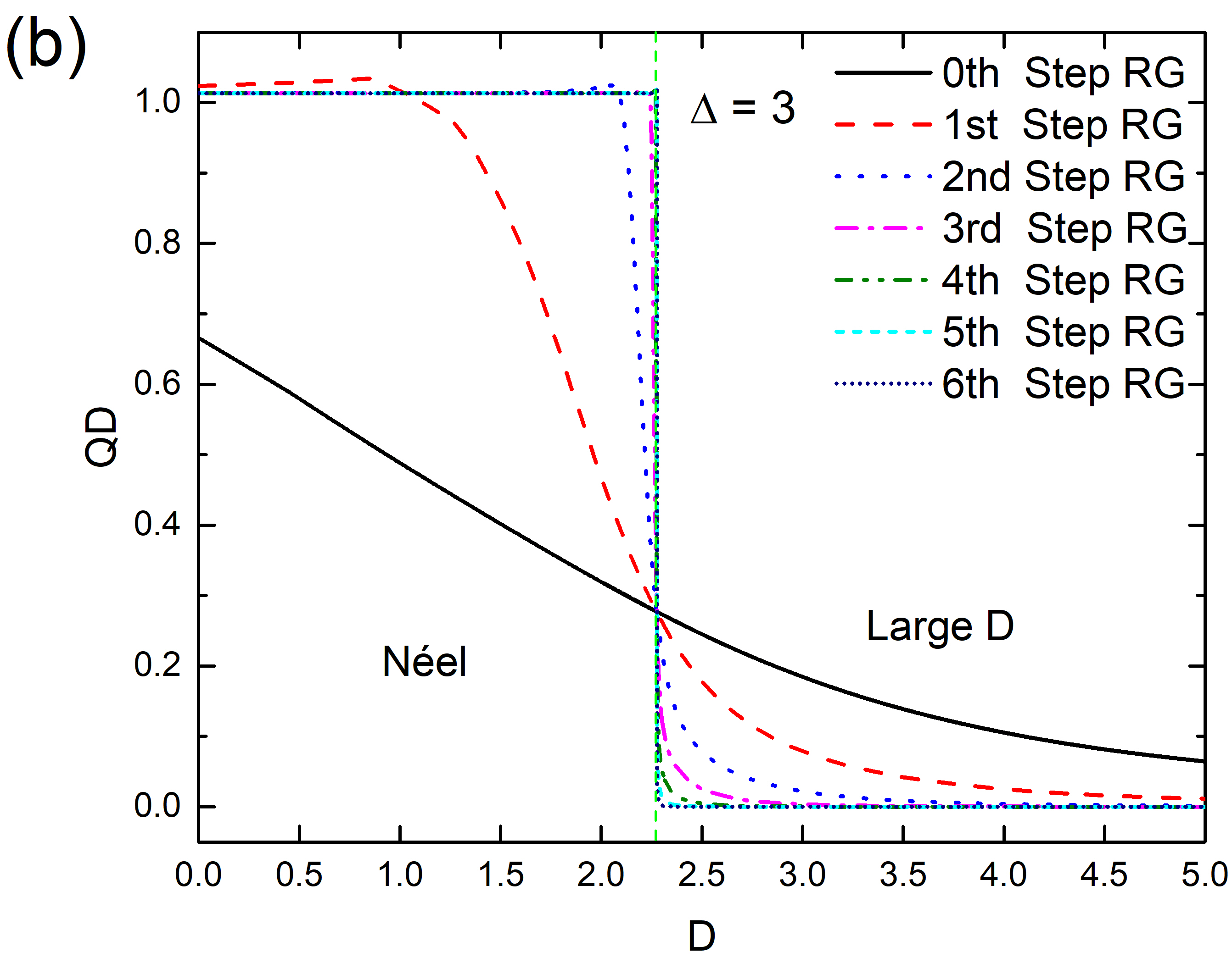
Figure 6: (a) Negativity and (b) QD in terms of QRG iterations at $\Delta=3$. Each phase is labelled by the black text, and separated by the dashed green line at $D=2.27$.

IV Nonanalytic and scaling behavior

The entanglement and QC usually present nonanalytic behaviors at the phase transition points, which are accompanied by scaling behavior due to the divergence of the correlation length. This section shows the QPT and nonanalytic behaviors of the negativity and QD in the spin-1 Heisenberg chain. We analyze the first partial derivative of negativity and QD with respect to the single-ion anisotropy parameter for a fixed value of $\bigtriangleup=0$. As shown in 7(a), the absolute value of the first partial derivative of the negativity, with respect to the single-ion anisotropy parameter, i.e., $\left|\partial N/\partial D\right|$, is discontinuous at the critical point $P_{4}(0,-1.91)$, and the singular behavior becomes more pronounced as the size of the system increases. However there is only a maximum at the critical point $P_{3}:(0,1.45)$, up to 6th step of RG, as shown in the inset of the same figure. The single-ion anisotropy parameter corresponds to the maximum of $\left|\partial N/\partial D\right|$ tends to the fixed point as the size of the system increases. The QD exhibits similar behavior with respect to the single-ion anisotropy parameter, i.e., $\left|\partial QD/\partial D\right|$, as shown in 7(b). For $\bigtriangleup=1$, $\left|\partial N/\partial D\right|$ shows a growing peak at the phase transition point $P_{1}:(1.0,0)$, and the position of the extreme point varies as the size of the system increases, which arises from finite-size effects. Note that, there is only a maximum at $P_{6}:(1.0,1.37)$ in the 6th step of the RG, as shown in figure 8(a). One can infer that, with enough RG iterations, both $\left|\partial N/\partial D\right|$ and $\left|\partial QD/\partial D\right|$ should also exhibit nonanalytic behavior at the boundary of Haldane and Large-D phases. Similar behavior of the QD with respect to $D$ for $\bigtriangleup=1$ are also obtained, as shown in figure 8(b). For $\bigtriangleup=3$, both $\left|\partial N/\partial D\right|$ and $\left|\partial QD/\partial D\right|$ are discontinuous at $P_{5}:(3.0,2.27)$, as shown in figure 9(a) and (b). For $D=0$, both $\left|\partial N/\partial\bigtriangleup\right|$ and $\left|\partial QD/\partial\bigtriangleup\right|$ also become discontinuous at $P_{1}:(1.0,0)$, as the size of the system increases, as shown in figure S3(a) and (b) of appendix B.

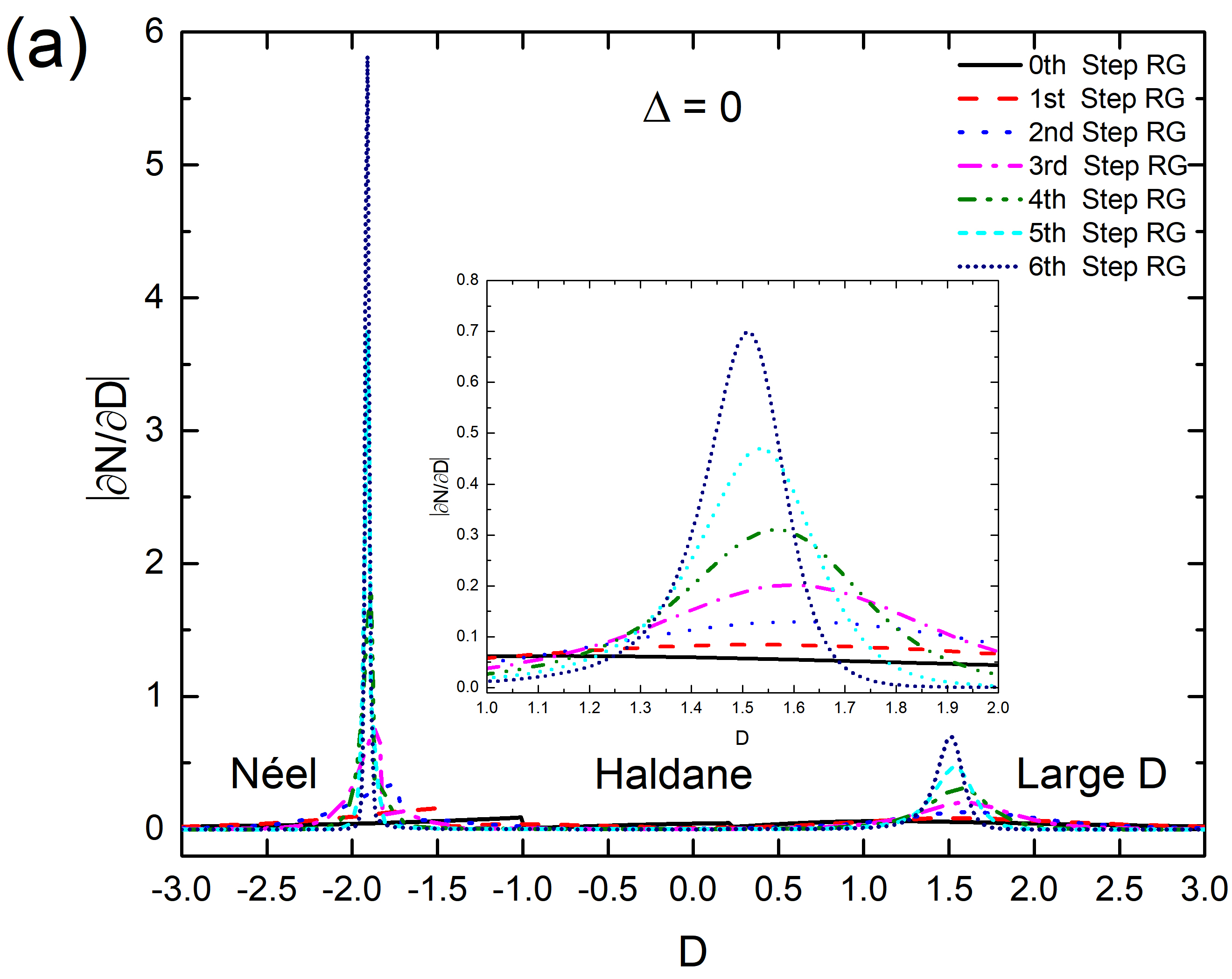
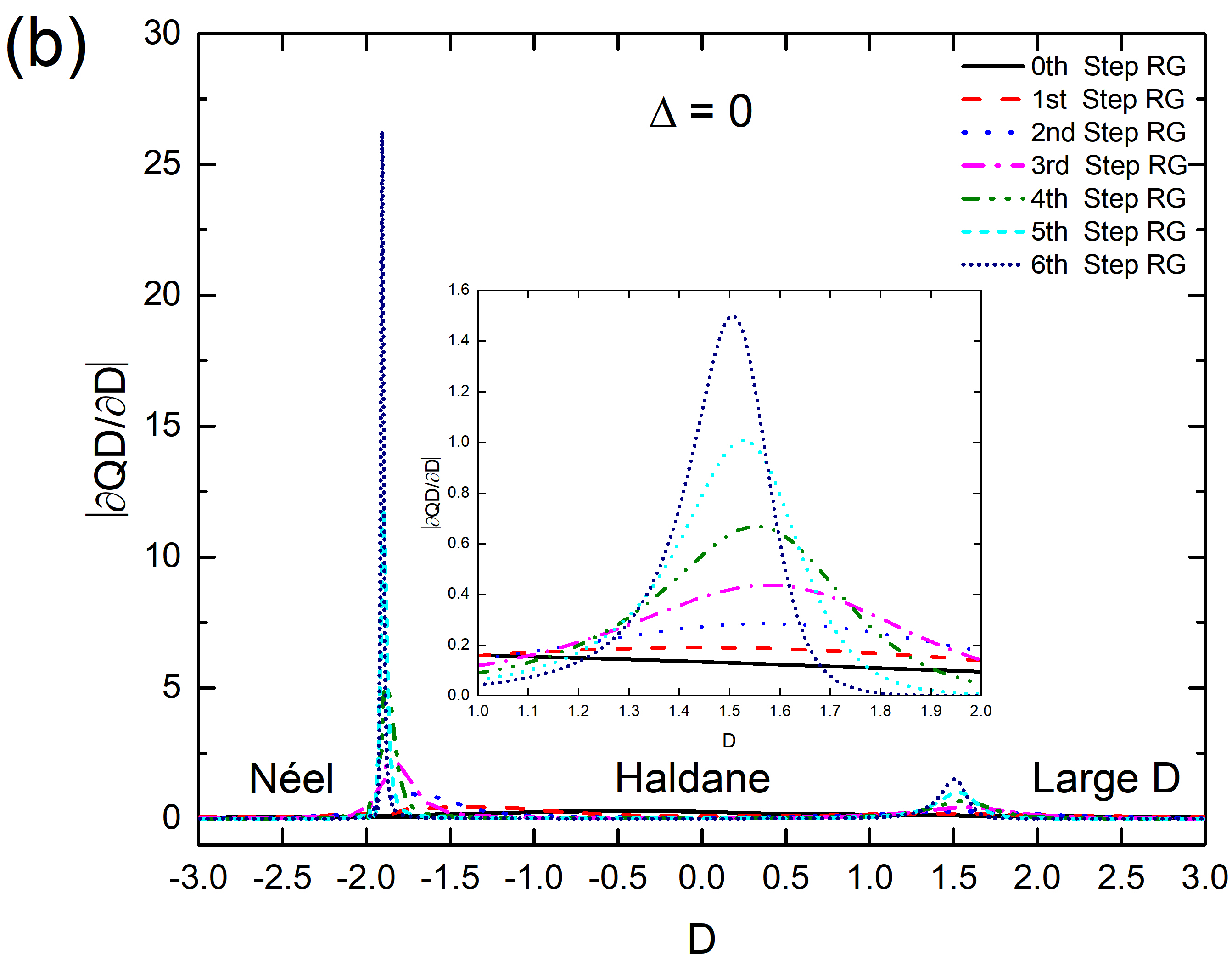
Figure 7: Absolute value of the first partial derivative of (a) negativity and (b) QD, with respect to $D$, as the step of the QRG iterations increases at $\Delta=0$ (figure 4(a) and (b)). Each phase is labelled by the black text.

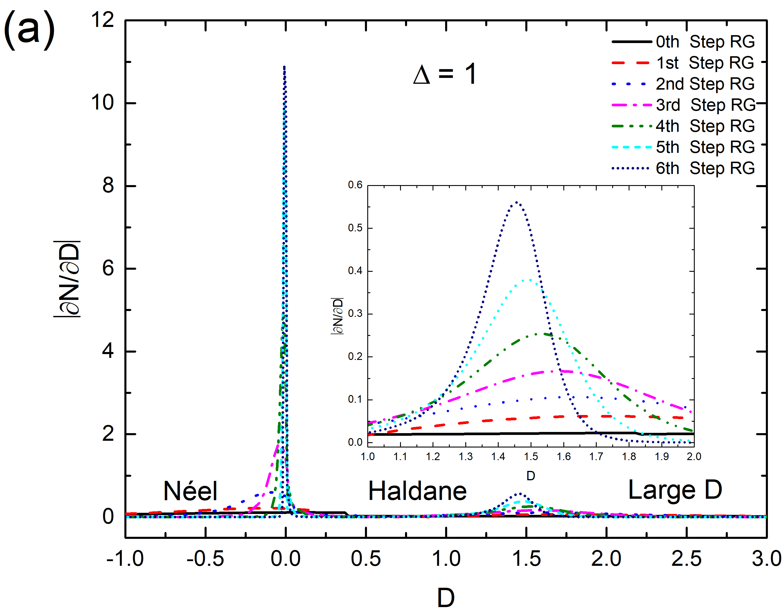
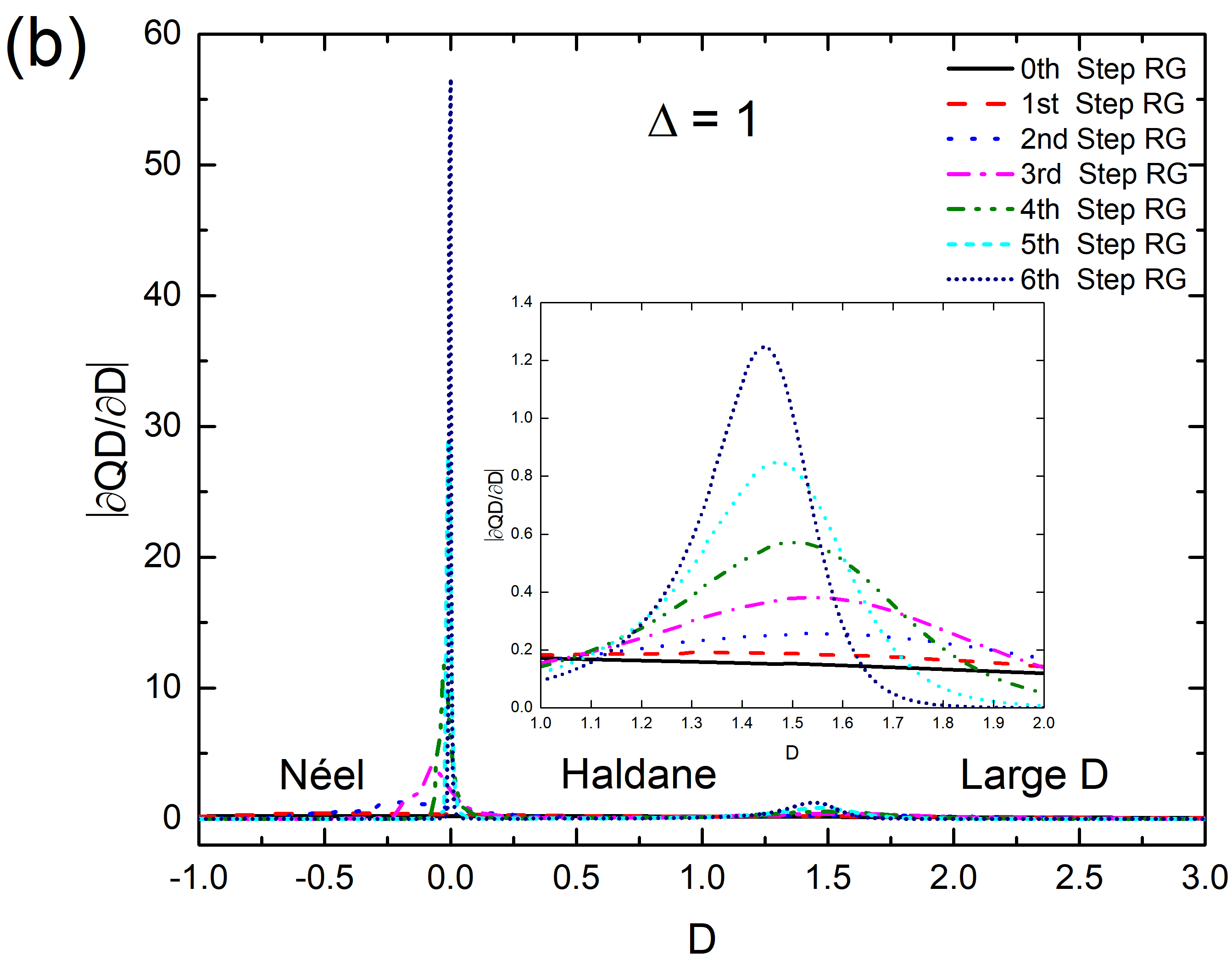
Figure 8: Absolute value of the first partial derivative of (a) negativity and (b) QD, with respect to $D$, as the step of the QRG iterations increases at $\Delta=1$ (figure 5(a) and (b)). Each phase is labelled by the black text.

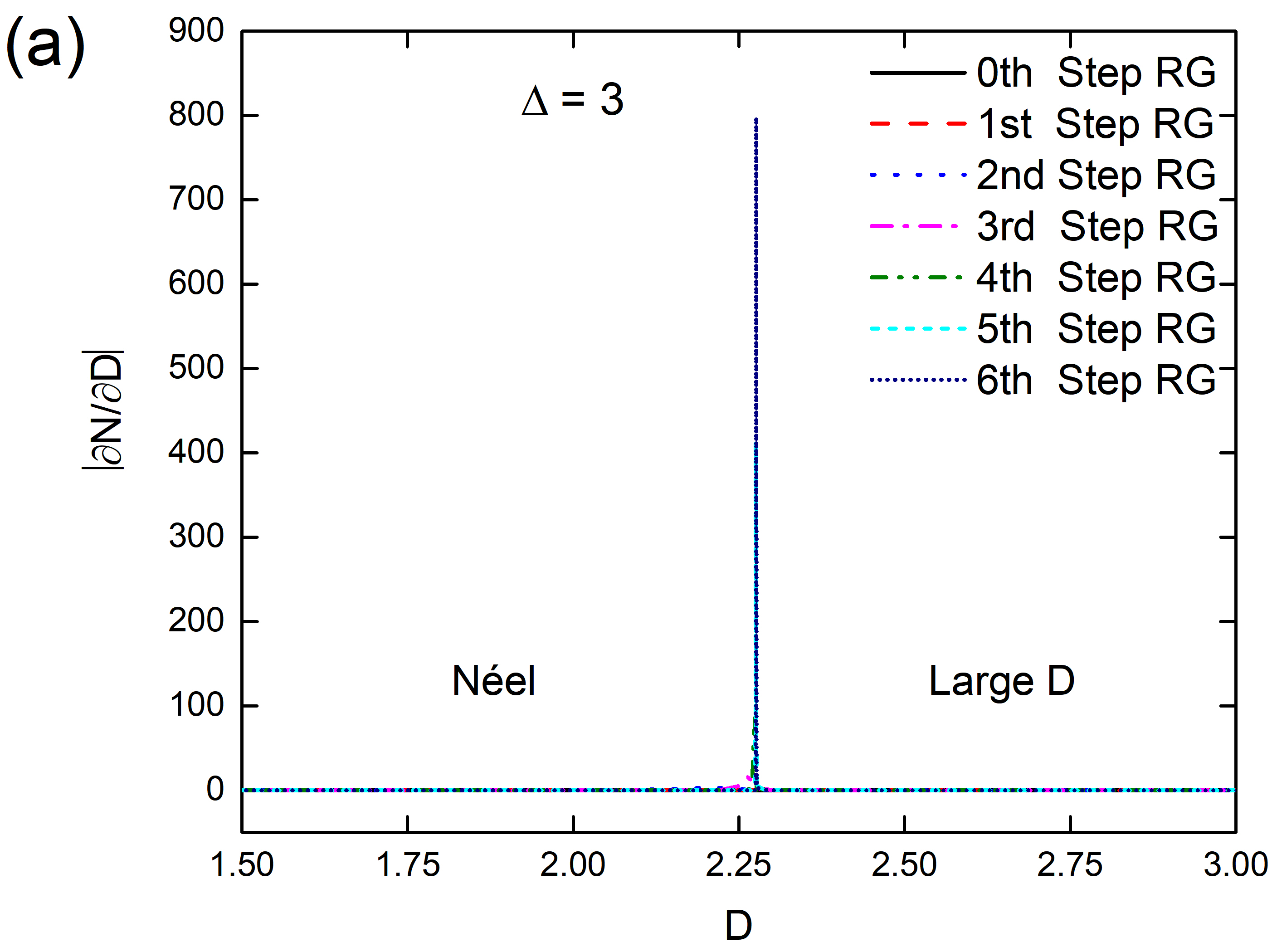
Figure 9: Absolute value of the first partial derivative of (a) negativity and (b) QD, with respect to $D$, as the step of the QRG iterations increases at $\Delta=3$ (figure 6(a) and (b)). Each phase is labelled by the black text.

The logarithm of the maximum of the absolute value of the first partial derivative of the negativity, with respect to the single-ion anisotropy $D$, i.e., $ln\left|\partial N/\partial D\right|_{max}$, versus the logarithm of the system size, i.e., $lnL$, obey the linear relation $\left|\partial N/\partial D\right|_{max}\sim L^{\theta}$ at the critical points $P_{4}(0,-1.91)$ and $P_{3}:(0,1.45)$. These are shown in figure 10(a) and (c), respectively. The singular behavior of the negativity and the scaling behavior of the system depend on the QC exponent $\theta$, as shown in Table 1. A similar linear relation, i.e., $\left|\partial QD/\partial D\right|_{max}\sim L^{\theta}$ is also obtained at the critical points $P_{4}(0,-1.91)$ and $P_{3}:(0,1.45)$, as shown in figure 10(b) and (d). The scaling behaviors of $ln\left|\partial N/\partial D\right|_{max}$ versus $lnL$ at $P_{1}:(1.0,0)$ and $P_{6}:(1.0,1.37)$ also exhibit linear relations, as shown in figure S4(a) and figure S5(a) of appendix B, respectively. Amazingly, for $D=0$, both $\left|\partial N/\partial\Delta\right|_{max}\sim L^{\theta}$ and $\left|\partial QD/\partial\Delta\right|_{max}\sim L^{\theta}$ have nearly the same relation at $P_{1}:(1.0,0)$, as shown in figure S6(a) and (b). The linear relation of $\left|\partial N/\partial D\right|_{max}\sim L^{\theta}$ at $P_{5}:(3.0,2.27)$ is shown in figure S7(a) of appendix B. Furthermore, the scaling behavior of $ln\left|\partial QD/\partial D\right|_{max}$ versus $lnL$ at the phase transition points $P_{1}:(1.0,0)$, $P_{6}:(1.0,1.37)$ and $P_{5}:(3.0,2.27)$ also exhibits the linear relations $\left|\partial QD/\partial D\right|_{max}\sim L^{\theta}$, as shown in figure S4(b), figure S5(b), and figure S7(b) of appendix B. The QC exponents $\theta$, calculated from the negativity and QD, are nearly equal at each fixed point.

:

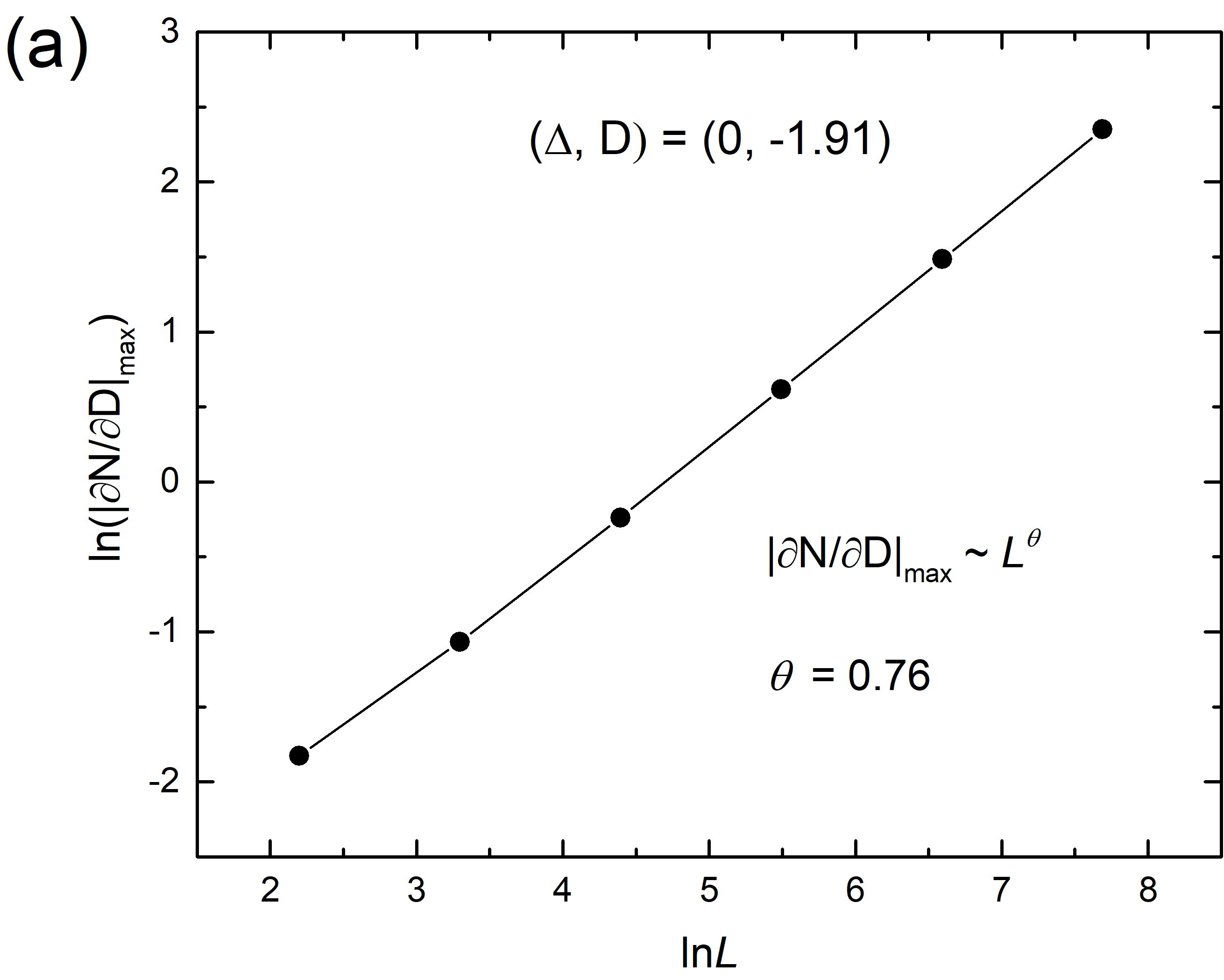
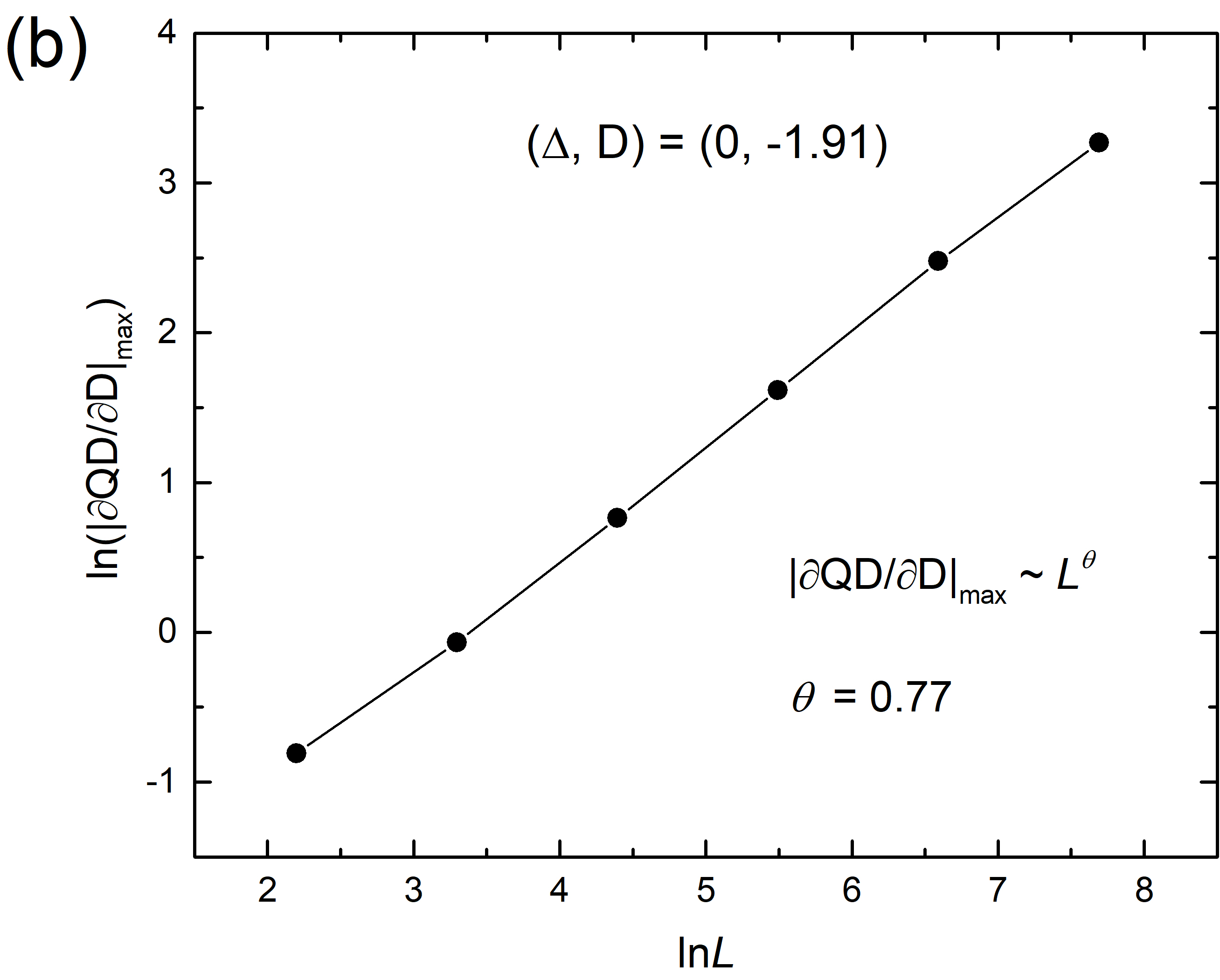
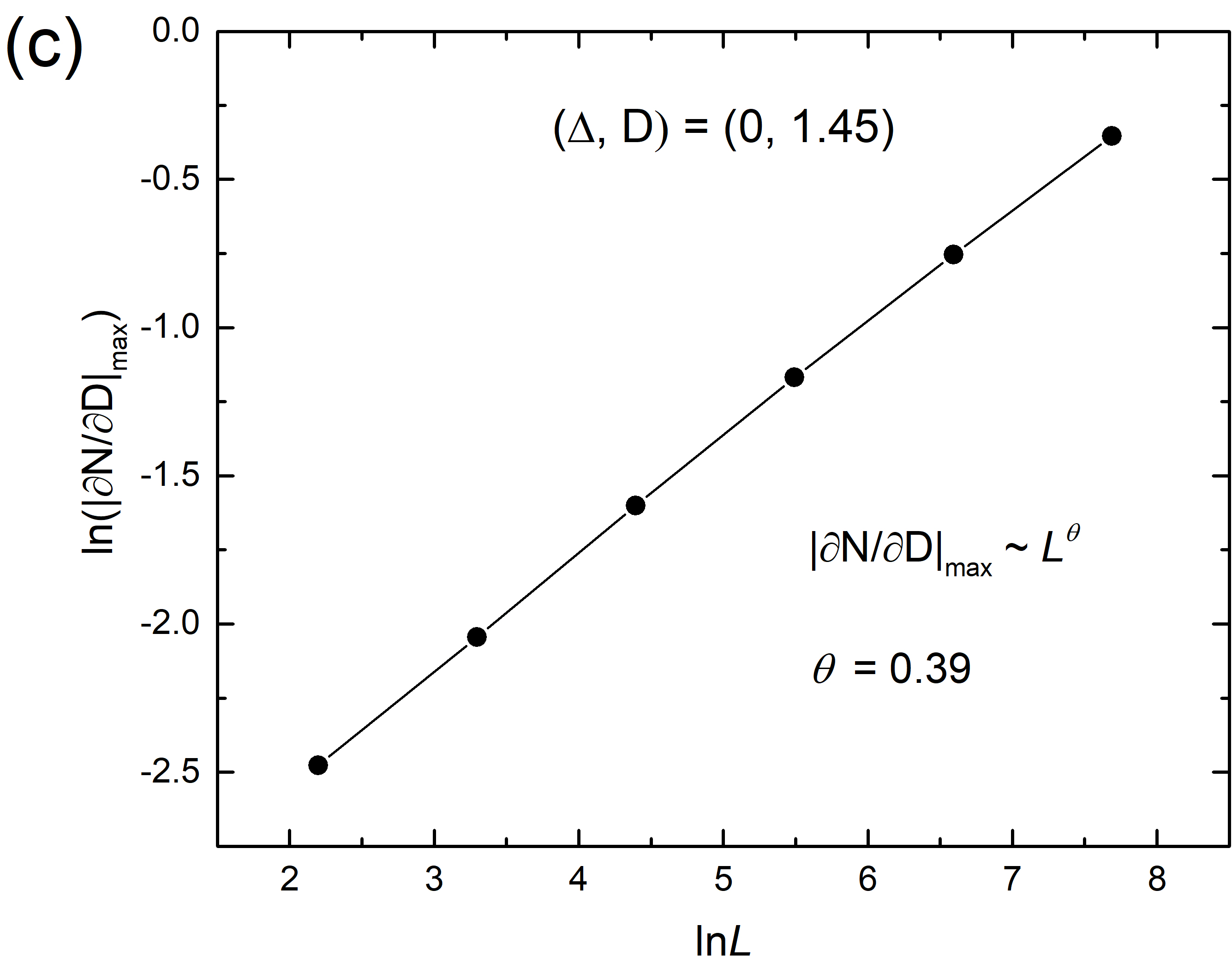
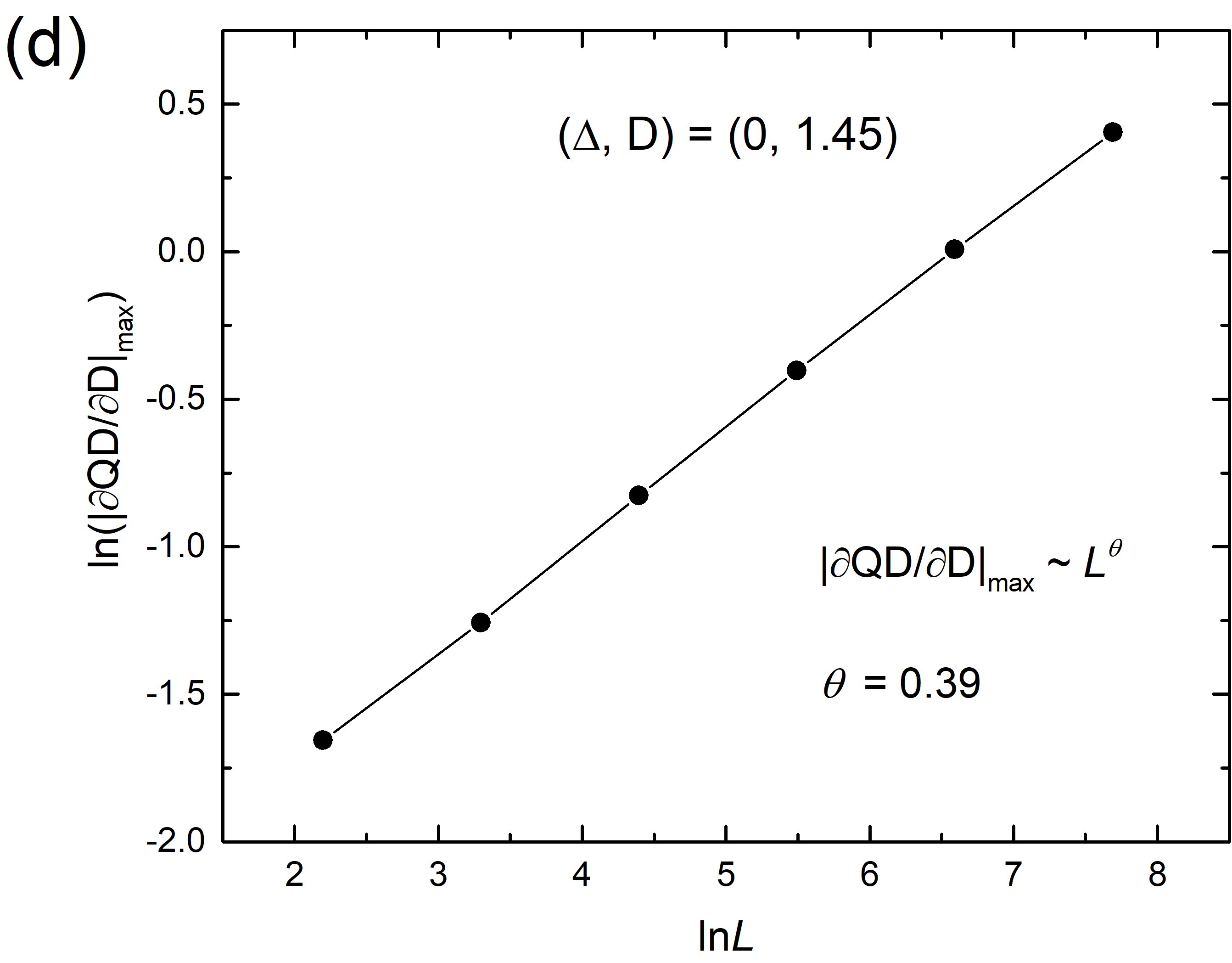
Figure 10: Logarithm of the maximum of (a) $\left|\partial N/\partial D\right|$ and (b) $\left|\partial QD/\partial D\right|$ versus the logarithm of the system size, $lnL$, at $P_{4}(0,-1.91)$. Logarithm of the maximum of (c) $\left|\partial N/\partial D\right|$ and (d) $\left|\partial QD/\partial D\right|$ versus $lnL$ at $P_{3}(0,1.45)$.

In the spin system, the correlation length $\xi$ becomes divergent as $\xi\sim|D-D_{c}|^{-\nu}$ at the critical point $D_{c}$ and the correlation length exponent $\nu$ can be obtained from the formula $\nu=\left[ln\left(n_{B}\right)\right]/ln\left[\partial D^{{}^{\prime}}/\partial D\right]$$|_{D_{c}}$, where $n_{B}$ is the number of spins in one block and $D^{{}^{\prime}}$ is the recurrence relation of the single-ion parameter $D$ in Eq.(4) Jafari et al. (2008); Martín-Delgado and Sierra (1996). In the Haldane-Néel transition at $P_{1}:(1.0,0)$, the entanglement exponent $\theta=1.01$ is nearly equal to that of the Néel-Haldane transition, i.e. $\theta=0.97$, which implies that both the Néel-Haldane and Haldane-Néel transitions at $P_{1}:(1.0,0)$ are in the same universality class, even though the correlation length exponent in the Haldane-Néel transition, $\nu=1.39$, is much smaller than that of the Néel-Haldane transition $\nu=3.12$. We can infer that, for a given fixed point, the phase transitions along different directions are in the same universality class. The type of phase transition, the QC exponent $\theta$, and the correlation length exponent $\nu$ at each fixed point are presented in Table 1. Amazingly, both at the critical points $P_{3}:(0,1.45)$ and $P_{4}:(0,-1.91)$, their QC exponent $\theta$ and the corresponding correlation length exponent $\nu$, are reciprocals, i.e., $\nu=\frac{1}{\theta}$. This is similar to the case of spin-1/2 systems Ma et al. (2011a, b). As the critical points are approaching the large-size limit (not the thermodynamic limit), the correlation length covers the whole system.

Table 1: The type of phase transition, QC exponent $\theta$, and the correlation length exponent $\nu$ of the spin-1 Heisenberg model at each fixed point $\left(\bigtriangleup,D\right)$. The subscripts $N$ and $QD$ indicate the results derived from negativity and QD, respectively.

$$(\bigtriangleup,D)$$ transition type

Néel-Haldane (Ising)

Haldane-large D (Gaussian)

Néel-Haldane (Ising)

Néel-large D (first-order)

Haldane-large D (Gaussian)

V Summary

The QCs and QPTs of the spin-1 Heisenberg chain with single-ion anisotropy were investigated using the QRG method. The phase diagram of the spin-1 system is more complex and richer than that of the spin-1/2 system, which is determined by the easy-axis anisotropy and single-ion anisotropy parameters. Both negativity and QD can equivalent to depict the QPT. The single-ion anisotropy parameter plays an important role in reducing the negativity and QD by favoring the alignment of spins. As the scale of the system increases, the negativity and QD exhibit step-like patterns in different phases. The critical behavior of the spin-1 chain was described by the first partial derivative of the negativity or QD of the blocks, which show nonanalytic behavior at the phase transition points. The QC exponent $\theta$ and correlation length exponent $\nu$ derived from negativity and QD are nearly equal at each fixed point. Notably, they are reciprocals, i.e. $\nu=\frac{1}{\theta}$, at the critical points $P_{3}:(0,1.45)$ and $P_{4}:(0,-1.91)$. This is similar to the case of spin-1/2 systems Jafari et al. (2008); Ma et al. (2011a, b) and our results are also consistent with previous work Langari et al. (2013). Better yet, the entanglement and QD show a clear QPT, even when the scale of spin-1 systems is as small as $3^{3}$ sites.

Appendix A The QRG procedure

The quantum renormalization group procedure can be reedited as shown below Langari et al. (2013):

To begin with, the lattice is decomposed into isolated blocks where the total Hamiltonian is written as a sum of isolated block Hamiltonians $\left(H^{B}\right)$ and inter-block interactions $\left(H^{BB}\right)$, i.e., $H=H^{B}+H^{BB}$, where, $H^{B}=\sum\nolimits_{I=1}^{L/3}h_{I}^{B}$, $H^{BB}=\sum\nolimits_{I=1}^{L/3}h_{I,I+1}^{BB}$, and

$$h_{I}^{B}=J\left[\sum_{j=1}^{2}\left(S_{I,j}^{x}S_{I,j+1}^{x}+S_{I,j}^{y}S_{I,j+1}^{y}+\bigtriangleup S_{I,j}^{z}S_{I,j+1}^{z}\right)+D\sum_{j=1}^{3}\left(S_{I,j}^{z}\right)^{2}\right],$$

$$h_{I,I+1}^{BB}=J\left(S_{I,3}^{x}S_{I+1,1}^{x}+S_{I,3}^{y}S_{I+1,1}^{y}+\bigtriangleup S_{I,3}^{z}S_{I+1,1}^{z}\right).$$

$S_{I,j}^{\alpha}$ denotes the $\alpha$-component of the $j$th spin in block $I$. The energy eigenstates of $h_{I}^{B}$ are calculated exactly and the three lowest eigenvectors are denoted by $\left|\phi_{0}\right\rangle$ and $\left|\phi_{\pm}\right\rangle$ with the corresponding eigenvalues $E_{0}$ and $E_{1}$, respectively.

In addition, the three low-lying energy eigenstates of each block are kept to build up an embedding (projection) operator $\left(T\right)$, representing the most important subspace of the original Hilbert space $\left(H\right)$. The embedding operator for each block is constructed as

$$T_{I}=\left|\phi_{+}\right\rangle\left\langle+1\right|+\left|\phi_{0}\right\rangle\left\langle 0\right|+\left|\phi_{-}\right\rangle\left\langle-1\right|,$$

where $\left|\pm 1\right\rangle,\left|0\right\rangle$ are the base kets for the renormalized Hilbert space of each block.

Finally, the original Hamiltonian $\left(H\right)$ is mapped into the renormalized Hamiltonian $\left(H^{{}^{\prime}}\right)$ utilizing the embedding operator, which is given by

$$H^{{}^{\prime}}=\sum_{I=1}^{L/3}\left(T_{I}^{\dagger}h_{I}^{B}T_{I}+T_{I}^{\dagger}T_{I+1}^{\dagger}h_{I,I+1}^{BB}T_{I+1}T_{I}\right).$$

The first part of the projections leads to

$$T_{I}^{\dagger}h_{I}^{B}T_{I}=E_{0}1+\left(E_{1}-E_{0}\right)\left(S_{I}^{z}\right)^{2},$$

and the second term of the projection defines the effective interaction between blocks $I$ and $I+1$ in terms of the renormalized operators,

$$T_{I}^{\dagger}S_{I,j}^{\alpha}T_{I}=X_{ren}S_{I}^{{}^{\prime\alpha}};~{}j=1,3;~{}\alpha=x,y,$$

$$T_{I}^{\dagger}S_{I,j}^{z}T_{I}=Z_{ren}S_{I}^{{}^{\prime z}};~{}j=1,3.$$

The renormalization coefficients $X_{ren}$ and $Z_{ren}$ are given by the following expressions,

$$X_{ren} =\frac{1}{\sqrt{A_{5}A_{9}}}[2\left(E_{0}-2D\right)+2\left(E_{1}-3D\right)$$

$$\times\left[4D^{2}-2D\left(\bigtriangleup+2E_{0}\right)+E_{0}\left(\bigtriangleup+E_{0}\right)-2\right]$$

$$-A_{2}A_{3}\left(D-E_{1}\right)[4D^{2}E_{0}-2A_{8}-2D$$

$$\times\left[E_{0}\left(\bigtriangleup+2E_{0}\right)-3\right]+E_{0}^{2}\left(\bigtriangleup+E_{0}\right)-6E_{0}]$$

$$+2A_{1}A_{2}A_{3}\left(A_{8}-D+E_{0}\right)$$

$$-\frac{A_{7}\left[A_{1}A_{2}A_{3}\left(D-E_{1}\right)-6D+2E_{1}\right]}{2D-E_{0}}],$$ (a8)

$$Z_{ren} =\frac{1}{A_{5}}[-[\left(D-E_{1}\right)[A_{1}A_{2}A_{3}\left(D-E_{1}\right)+4E_{1}-12D]+2]^{2}$$

$$+4\left(E_{1}-3D\right)^{2}+4+A_{3}^{2}A_{2}^{2}\left(D-E_{1}\right)^{2}].$$ (a9)

The constants $A_{i}$ are given by:

$$A_{1}=2\bigtriangleup-3D+E_{1},$$ (a10)

$$A_{2}=E_{1}^{2}-4DE_{1}+3D^{2}-1,$$ (a11)

$$A_{3}=\frac{1}{\bigtriangleup-2D+E_{1}},$$ (a12)

$$A_{4}=\frac{1}{\bigtriangleup-2D+E_{0}},$$ (a13)

$$A_{5} =A_{3}^{2}\left[A_{1}A_{2}\left(D-E_{1}\right)+2\left(3D-E_{1}\right)\left(2D-\bigtriangleup-E_{2}\right)\right]^{2}$$

$$+A_{2}^{2}A_{3}^{2}\left(D-E_{1}\right)^{2}+A_{1}^{2}A_{2}^{2}A_{3}^{2}+4\left(E_{1}-3D\right)^{2}+4$$

$$+\left[\left(D-E_{1}\right)\left[A_{1}A_{2}A_{3}\left(D-E_{1}\right)+4\left(E_{1}-3D\right)\right]+2\right]^{2},$$ (a14)

$$A_{6} =16D^{4}E_{0}-8D^{3}\left[2E_{0}\left(\bigtriangleup+2E_{0}\right)-3\right]$$

$$+4D^{2}\left[6E_{0}^{3}+6\bigtriangleup E_{0}^{2}+\left(\bigtriangleup^{2}-12\right)E_{0}-3\bigtriangleup\right]$$

$$-2D\left[4E_{0}^{4}+6\bigtriangleup E_{0}^{3}+\left(2\bigtriangleup^{2}-15\right)E_{0}^{2}-9\bigtriangleup E_{0}+4\right]$$

$$+E_{0}^{2}\left(\bigtriangleup+E_{0}\right)\left[E_{0}\left(\bigtriangleup+E_{0}\right)-6\right]+6E_{0},$$ (a15)

$$A_{7}=-E_{0}^{3}+E_{0}^{2}\left(4D-\bigtriangleup\right)+2E_{0}\left(D\bigtriangleup-2D^{2}\right)-4D+2,$$ (a16)

$$A_{8}=\frac{A_{4}\left(3E_{0}-4D\right)}{2D-E_{0}},$$ (a17)

$$A_{9} =\frac{A_{4}^{2}A_{6}^{2}+A_{7}^{2}}{\left(E_{0}-2D\right)^{2}}+2\left(E_{0}-2D\right)^{2}+4\left(A_{8}-D+E_{0}\right)^{2}+4$$

$$+\left[4D^{2}-2D\left(\bigtriangleup+2E_{0}\right)+E_{0}\left(\bigtriangleup+E_{0}\right)-2\right]^{2}.$$ (a18)

The renormalized coupling constants can be obtained as shown in Eqs.(2)(3)(4) of the text.

Appendix B The Figures

See figures S1, S2, S3, S4, S5, S6 and S7.

Figure S1. (a) The quantum mutual information (QMI) between the first and third sites of the three-site model in terms of the single-ion anisotropy $D$ for different $\Delta$. (b) The quantum mutual information in terms of the QRG iterations at $\Delta=0$. Each phase is marked by the black text, and separated by the dashed green lines at $D=-1.91$ and $D=1.45$, respectively.

Figure S2. (a) Negativity and (b) QD in terms of the QRG iterations at $D=0$. Each phase is marked by the black text, and separated by the dashed green line at $\Delta=1.0$.

Figure S3. Absolute value of the first partial derivative of (a) negativity and (b) QD, with respect to $\Delta$, as the step of the QRG iterations increases at $D=0$ (figure S2(a) and (b)). Each phase is labelled by the black text.

Figure S4. Logarithm of the maximum of (a) $\left|\partial N/\partial D\right|$ and (b) $\left|\partial QD/\partial D\right|$ versus the logarithm of the system size, $lnL$, at $P_{1}:(1.0,0)$.

Figure S5. Logarithm of the maximum of (a) $\left|\partial N/\partial D\right|$ and (b) $\left|\partial QD/\partial D\right|$ versus the logarithm of the system size, $lnL$, at $P_{6}:(1.0,1.37)$.

Figure S6. Logarithm of the maximum of (a) $\left|\partial N/\partial\Delta\right|$ and (b) $\left|\partial QD/\partial\Delta\right|$ versus the logarithm of the system size, $lnL$, at $P_{1}:(1.0,0)$.

Figure S7. Logarithm of the maximum of (a) $\left|\partial N/\partial D\right|$ and (b) $\left|\partial QD/\partial D\right|$ versus the logarithm of the system size, $lnL$, at $P_{5}:(3.0,2.27)$.

References

- Bennett et al. (1993) Charles H. Bennett, Gilles Brassard, Claude Crépeau, Richard Jozsa, Asher Peres, and William K. Wootters. Teleporting an unknown quantum state via dual classical and Einstein-Podolsky-Rosen channels. Phys. Rev. Lett., 70:1895–1899, Mar 1993. doi: 10.1103/PhysRevLett.70.1895. URL https://link.aps.org/doi/10.1103/PhysRevLett.70.1895.
- Zheng and Guo (2000) Shi-Biao Zheng and Guang-Can Guo. Efficient scheme for two-atom entanglement and quantum information processing in cavity QED. Phys. Rev. Lett., 85:2392–2395, Sep 2000. doi: 10.1103/PhysRevLett.85.2392. URL https://link.aps.org/doi/10.1103/PhysRevLett.85.2392.
- Ekert (1991) Artur K. Ekert. Quantum cryptography based on Bell’s theorem. Phys. Rev. Lett., 67:661–663, Aug 1991. doi: 10.1103/PhysRevLett.67.661. URL https://link.aps.org/doi/10.1103/PhysRevLett.67.661.
- Bouwmeester et al. (1997) Dik Bouwmeester, Jian-Wei Pan, Klaus Mattle, Manfred Eibl, Harald Weinfurter, and Anton Zeilinger. Experimental quantum teleportation. Nature, 390(6660):575–579, 1997.
- Hill and Wootters (1997) Scott Hill and William K. Wootters. Entanglement of a pair of quantum bits. Phys. Rev. Lett., 78:5022–5025, Jun 1997. doi: 10.1103/PhysRevLett.78.5022. URL https://link.aps.org/doi/10.1103/PhysRevLett.78.5022.
- Osterloh et al. (2002) Andreas Osterloh, Luigi Amico, Giuseppe Falci, and Rosario Fazio. Scaling of entanglement close to a quantum phase transition. Nature, 416(6881):608–610, 2002.
- Vidal et al. (2003) G. Vidal, J. I. Latorre, E. Rico, and A. Kitaev. Entanglement in quantum critical phenomena. Phys. Rev. Lett., 90:227902, Jun 2003. doi: 10.1103/PhysRevLett.90.227902. URL https://link.aps.org/doi/10.1103/PhysRevLett.90.227902.
- Verstraete et al. (2004) F. Verstraete, M. Popp, and J. I. Cirac. Entanglement versus correlations in spin systems. Phys. Rev. Lett., 92:027901, Jan 2004. doi: 10.1103/PhysRevLett.92.027901. URL https://link.aps.org/doi/10.1103/PhysRevLett.92.027901.
- Ollivier and Zurek (2001) Harold Ollivier and Wojciech H. Zurek. Quantum discord: A measure of the quantumness of correlations. Phys. Rev. Lett., 88:017901, Dec 2001. doi: 10.1103/PhysRevLett.88.017901. URL https://link.aps.org/doi/10.1103/PhysRevLett.88.017901.
- Chen et al. (2011) Qing Chen, Chengjie Zhang, Sixia Yu, X. X. Yi, and C. H. Oh. Quantum discord of two-qubit states. Phys. Rev. A, 84:042313, Oct 2011. doi: 10.1103/PhysRevA.84.042313. URL https://link.aps.org/doi/10.1103/PhysRevA.84.042313.
- Sachdev (2007) Subir Sachdev. Quantum phase transitions. Handbook of Magnetism and Advanced Magnetic Materials, 2007.
- Osborne and Nielsen (2002) Tobias J. Osborne and Michael A. Nielsen. Entanglement in a simple quantum phase transition. Phys. Rev. A, 66:032110, Sep 2002. doi: 10.1103/PhysRevA.66.032110. URL https://link.aps.org/doi/10.1103/PhysRevA.66.032110.
- Wilson (1975) Kenneth G. Wilson. The renormalization group: Critical phenomena and the Kondo problem. Rev. Mod. Phys., 47:773–840, Oct 1975. doi: 10.1103/RevModPhys.47.773. URL https://link.aps.org/doi/10.1103/RevModPhys.47.773.
- Burkhardt and van Leeuwen (2012) Theodore W Burkhardt and JMJ van Leeuwen. Real-space renormalization, volume 30. Springer Science & Business Media, 2012.
- White (1992) Steven R. White. Density matrix formulation for quantum renormalization groups. Phys. Rev. Lett., 69:2863–2866, Nov 1992. doi: 10.1103/PhysRevLett.69.2863. URL https://link.aps.org/doi/10.1103/PhysRevLett.69.2863.
- Xiang (1996) T. Xiang. Density-matrix renormalization-group method in momentum space. Phys. Rev. B, 53:R10445–R10448, Apr 1996. doi: 10.1103/PhysRevB.53.R10445. URL https://link.aps.org/doi/10.1103/PhysRevB.53.R10445.
- Tzeng and Yang (2008) Yu-Chin Tzeng and Min-Fong Yang. Scaling properties of fidelity in the spin-1 anisotropic model. Phys. Rev. A, 77:012311, Jan 2008. doi: 10.1103/PhysRevA.77.012311. URL https://link.aps.org/doi/10.1103/PhysRevA.77.012311.
- Gong et al. (2015) Shou-Shu Gong, Wei Zhu, and D. N. Sheng. Quantum phase diagram of the spin-1 heisenberg model on the honeycomb lattice. Phys. Rev. B, 92:195110, Nov 2015. doi: 10.1103/PhysRevB.92.195110. URL https://link.aps.org/doi/10.1103/PhysRevB.92.195110.
- Zhang et al. (2017) Guo-Qing Zhang, Wei Wu, and Jing-Bo Xu. Multipartite entanglement from matrix-product states and a quantum phase transition. Phys. Rev. A, 96:032302, Sep 2017. doi: 10.1103/PhysRevA.96.032302. URL https://link.aps.org/doi/10.1103/PhysRevA.96.032302.
- Verstraete and Cirac (2004) Frank Verstraete and J Ignacio Cirac. Renormalization algorithms for quantum-many body systems in two and higher dimensions. arXiv preprint cond-mat/0407066, 2004.
- Li et al. (2011) Wei Li, Shi-Ju Ran, Shou-Shu Gong, Yang Zhao, Bin Xi, Fei Ye, and Gang Su. Linearized tensor renormalization group algorithm for the calculation of thermodynamic properties of quantum lattice models. Phys. Rev. Lett., 106:127202, Mar 2011. doi: 10.1103/PhysRevLett.106.127202. URL https://link.aps.org/doi/10.1103/PhysRevLett.106.127202.
- Li et al. (2019) Han Li, Bin-Bin Chen, Ziyu Chen, Jan von Delft, Andreas Weichselbaum, and Wei Li. Thermal tensor renormalization group simulations of square-lattice quantum spin models. Phys. Rev. B, 100:045110, Jul 2019. doi: 10.1103/PhysRevB.100.045110. URL https://link.aps.org/doi/10.1103/PhysRevB.100.045110.
- Langari (2004) A. Langari. Quantum renormalization group of model in a transverse magnetic field. Phys. Rev. B, 69:100402, Mar 2004. doi: 10.1103/PhysRevB.69.100402. URL https://link.aps.org/doi/10.1103/PhysRevB.69.100402.
- Kargarian et al. (2008) M. Kargarian, R. Jafari, and A. Langari. Renormalization of entanglement in the anisotropic heisenberg model. Phys. Rev. A, 77:032346, Mar 2008. doi: 10.1103/PhysRevA.77.032346. URL https://link.aps.org/doi/10.1103/PhysRevA.77.032346.
- Jafari et al. (2008) R. Jafari, M. Kargarian, A. Langari, and M. Siahatgar. Phase diagram and entanglement of the Ising model with Dzyaloshinskii-Moriya interaction. Phys. Rev. B, 78:214414, Dec 2008. doi: 10.1103/PhysRevB.78.214414. URL https://link.aps.org/doi/10.1103/PhysRevB.78.214414.
- Xu et al. (2014) Yu-Liang Xu, Xin Zhang, Zhong-Qiang Liu, Xiang-Mu Kong, and Ting-Qi Ren. Robust thermal quantum correlation and quantum phase transition of spin system on fractal lattices. The European Physical Journal B, 87(6):132, 2014.
- Xu et al. (2016) Yu-Liang Xu, Xiang-Mu Kong, Zhong-Qiang Liu, and Chun-Yang Wang. Quantum entanglement and quantum phase transition for the ising model on a two-dimension square lattice. Physica A: Statistical Mechanics and its Applications, 446:217–223, 2016.
- Farajollahpour and Jafari (2018) T. Farajollahpour and S. A. Jafari. Topological phase transition of the anisotropic model with Dzyaloshinskii-Moriya interaction. Phys. Rev. B, 98:085136, Aug 2018. doi: 10.1103/PhysRevB.98.085136. URL https://link.aps.org/doi/10.1103/PhysRevB.98.085136.
- Ma et al. (2011a) Fu-Wu Ma, Sheng-Xin Liu, and Xiang-Mu Kong. Entanglement and quantum phase transition in the one-dimensional anisotropic model. Phys. Rev. A, 83:062309, Jun 2011a. doi: 10.1103/PhysRevA.83.062309. URL https://link.aps.org/doi/10.1103/PhysRevA.83.062309.
- Ma et al. (2011b) Fu-Wu Ma, Sheng-Xin Liu, and Xiang-Mu Kong. Quantum entanglement and quantum phase transition in the model with staggered Dzyaloshinskii-Moriya interaction. Phys. Rev. A, 84:042302, Oct 2011b. doi: 10.1103/PhysRevA.84.042302. URL https://link.aps.org/doi/10.1103/PhysRevA.84.042302.
- Xu et al. (2017) Yu-Liang Xu, Xiang-Mu Kong, Zhong-Qiang Liu, and Chuan-Cun Yin. Scaling of entanglement during the quantum phase transition for Ising spin systems on triangular and Sierpiński fractal lattices. Phys. Rev. A, 95:042327, Apr 2017. doi: 10.1103/PhysRevA.95.042327. URL https://link.aps.org/doi/10.1103/PhysRevA.95.042327.
- Cheng and Xu (2018) Jun-Qing Cheng and Jing-Bo Xu. Multipartite entanglement, quantum coherence, and quantum criticality in triangular and Sierpiński fractal lattices. Phys. Rev. E, 97:062134, Jun 2018. doi: 10.1103/PhysRevE.97.062134. URL https://link.aps.org/doi/10.1103/PhysRevE.97.062134.
- Regnault et al. (1994) L. P. Regnault, I. Zaliznyak, J. P. Renard, and C. Vettier. Inelastic-neutron-scattering study of the spin dynamics in the Haldane-gap system Ni(. Phys. Rev. B, 50:9174–9187, Oct 1994. doi: 10.1103/PhysRevB.50.9174. URL https://link.aps.org/doi/10.1103/PhysRevB.50.9174.
- Zheludev et al. (1996) A. Zheludev, S. E. Nagler, S. M. Shapiro, L. K. Chou, D. R. Talham, and M. W. Meisel. Spin dynamics in the linear-chain S=1 antiferromagnet Ni((). Phys. Rev. B, 53:15004–15009, Jun 1996. doi: 10.1103/PhysRevB.53.15004. URL https://link.aps.org/doi/10.1103/PhysRevB.53.15004.
- Asaad et al. (2020) Serwan Asaad, Vincent Mourik, Benjamin Joecker, Mark AI Johnson, Andrew D Baczewski, Hannes R Firgau, Mateusz T Mądzik, Vivien Schmitt, Jarryd J Pla, Fay E Hudson, et al. Coherent electrical control of a single high-spin nucleus in silicon. Nature, 579(7798):205–209, 2020.
- Schulz (1986) H. J. Schulz. Phase diagrams and correlation exponents for quantum spin chains of arbitrary spin quantum number. Phys. Rev. B, 34:6372–6385, Nov 1986. doi: 10.1103/PhysRevB.34.6372. URL https://link.aps.org/doi/10.1103/PhysRevB.34.6372.
- Chen et al. (2003) Wei Chen, Kazuo Hida, and B. C. Sanctuary. Ground-state phase diagram of chains with uniaxial single-ion-type anisotropy. Phys. Rev. B, 67:104401, Mar 2003. doi: 10.1103/PhysRevB.67.104401. URL https://link.aps.org/doi/10.1103/PhysRevB.67.104401.
- Hu et al. (2011) Shijie Hu, B. Normand, Xiaoqun Wang, and Lu Yu. Accurate determination of the Gaussian transition in spin-1 chains with single-ion anisotropy. Phys. Rev. B, 84:220402, Dec 2011. doi: 10.1103/PhysRevB.84.220402. URL https://link.aps.org/doi/10.1103/PhysRevB.84.220402.
- Ren et al. (2018) Jie Ren, Yimin Wang, and Wen-Long You. Quantum phase transitions in spin-1 chains with rhombic single-ion anisotropy. Phys. Rev. A, 97:042318, Apr 2018. doi: 10.1103/PhysRevA.97.042318. URL https://link.aps.org/doi/10.1103/PhysRevA.97.042318.
- Langari et al. (2013) A Langari, F Pollmann, and M Siahatgar. Ground-state fidelity of the spin-1 Heisenberg chain with single ion anisotropy: quantum renormalization group and exact diagonalization approaches. Journal of Physics: Condensed Matter, 25(40):406002, 2013.
- Huang et al. (2021) Jun-Han Huang, Guang-Ming Zhang, and Dao-Xin Yao. Dynamical spin excitations of the topological haldane gapped phase in the Heisenberg antiferromagnetic chain with single-ion anisotropy. Phys. Rev. B, 103:024403, Jan 2021. doi: 10.1103/PhysRevB.103.024403. URL https://link.aps.org/doi/10.1103/PhysRevB.103.024403.
- Wootters (1998) William K. Wootters. Entanglement of formation of an arbitrary state of two qubits. Phys. Rev. Lett., 80:2245–2248, Mar 1998. doi: 10.1103/PhysRevLett.80.2245. URL https://link.aps.org/doi/10.1103/PhysRevLett.80.2245.
- Vidal and Werner (2002) G. Vidal and R. F. Werner. Computable measure of entanglement. Phys. Rev. A, 65:032314, Feb 2002. doi: 10.1103/PhysRevA.65.032314. URL https://link.aps.org/doi/10.1103/PhysRevA.65.032314.
- Miranowicz and Grudka (2004) Adam Miranowicz and Andrzej Grudka. Ordering two-qubit states with concurrence and negativity. Phys. Rev. A, 70:032326, Sep 2004. doi: 10.1103/PhysRevA.70.032326. URL https://link.aps.org/doi/10.1103/PhysRevA.70.032326.
- Groisman et al. (2005) Berry Groisman, Sandu Popescu, and Andreas Winter. Quantum, classical, and total amount of correlations in a quantum state. Phys. Rev. A, 72:032317, Sep 2005. doi: 10.1103/PhysRevA.72.032317. URL https://link.aps.org/doi/10.1103/PhysRevA.72.032317.
- Malvezzi et al. (2016) A. L. Malvezzi, G. Karpat, B. Çakmak, F. F. Fanchini, T. Debarba, and R. O. Vianna. Quantum correlations and coherence in spin-1 Heisenberg chains. Phys. Rev. B, 93:184428, May 2016. doi: 10.1103/PhysRevB.93.184428. URL https://link.aps.org/doi/10.1103/PhysRevB.93.184428.
- Huang and Lin (2010) Ching-Yu Huang and Feng-Li Lin. Multipartite entanglement measures and quantum criticality from matrix and tensor product states. Phys. Rev. A, 81:032304, Mar 2010. doi: 10.1103/PhysRevA.81.032304. URL https://link.aps.org/doi/10.1103/PhysRevA.81.032304.
- Martín-Delgado and Sierra (1996) Miguel A. Martín-Delgado and Germán Sierra. Analytic formulations of the density matrix renormalization group. International Journal of Modern Physics A, 11(17):3145–3174, 1996. doi: 10.1142/S0217751X96001516. URL https://doi.org/10.1142/S0217751X96001516.