Statistically Robust, Risk-Averse Best Arm Identification in Multi-Armed Bandits

Abstract

Traditional multi-armed bandit (MAB) formulations usually make certain assumptions about the underlying arms’ distributions, such as bounds on the support or their tail behaviour. Moreover, such parametric information is usually ‘baked’ into the algorithms. In this paper, we show that specialized algorithms that exploit such parametric information are prone to inconsistent learning performance when the parameter is misspecified. Our key contributions are twofold: (i) We establish fundamental performance limits of statistically robust MAB algorithms under the fixed-budget pure exploration setting, and (ii) We propose two classes of algorithms that are asymptotically near-optimal. Additionally, we consider a risk-aware criterion for best arm identification, where the objective associated with each arm is a linear combination of the mean and the conditional value at risk (CVaR). Throughout, we make a very mild ‘bounded moment’ assumption, which lets us work with both light-tailed and heavy-tailed distributions within a unified framework.

I Introduction

The multi-armed bandit (MAB) problem is fundamental in online learning, where an optimal option needs to be identified among a pool of available options. Each option (or arm) generates a random reward/cost when chosen (or pulled) from an underlying unknown distribution, and the goal is to quickly identify the optimal arm by exploring all possibilities.

Classically, MAB formulations consider reward distributions with bounded support, typically $[0,1].$ Moreover, the support is assumed to be known beforehand, and this knowledge is baked into the algorithm. However, in many applications, it is more natural to not assume bounded support for the reward distributions, either because the distributions are themselves unbounded (even heavy-tailed), or because a bound on the support is not known a priori. There is some literature on MAB formulations with (potentially) unbounded rewards; see, for example, [2, 3]. Typically, in these papers, the assumption of a known bound on the support of the reward distributions is replaced with the assumption that certain bounds on the moments/tails of the reward distributions are known. Additionally, some algorithms even require knowledge of a lower bound on the sub-optimality gap between arms; see, for example, [4]. However, such prior information may not always be available. Even if available, it is likely to be unreliable, given that moment/tail bounds are typically themselves estimates based on limited data. Unfortunately, the effect of the unavailability/unreliability of such prior information on the performance of MAB algorithms has remained largely unexplored in the literature.

As we show in this paper, the performance of MAB algorithms is quite sensitive to the reliability of moment/tail bounds on arm distributions that have been incorporated into them. Specifically, we prove that such specialized algorithms can be inconsistent when presented with an MAB instance that violates the assumed moment bounds. This motivates the design of statistically robust MAB algorithms, i.e., algorithms that guarantee consistency on any MAB instance. This requirement ensures that algorithms are robust to misspecification of distributional parameters, and are not ‘over-specialized’ for a narrow class of parametrized instances.

Furthermore, the typical metric used to quantify the goodness of an arm in the MAB framework is its expected return, which is a risk-neutral metric. In some applications, particularly in finance, one is interested in balancing the expected return of an arm with the risk associated with that arm. This is particularly relevant when the underlying reward distributions are unbounded, even heavy-tailed, as is found to be the case with portfolio returns in finance; see [5]. In these settings, there is a non-trivial probability of a ‘catastrophic’ outcome, which motivates a risk-aware approach to optimal arm selection.

In this paper, we seek to address the two issues described above. Specifically, we consider the problem of identifying the arm that optimizes a linear combination of the mean and the Conditional Value at Risk (CVaR) in a fixed budget (pure exploration) MAB framework. Considering a mean-CVaR framework provides some flexibility to trade-off between risk-aversion and reward-seeking behavior. It is similar in spirit to considering the popular mean-variance formulation. However, CVaR is a better-behaved risk metric (see [6]) compared to variance, in addition to having the same dimensional units as the mean loss. Moreover, the existence of CVaR requires only the first moment to be well defined, while existence of variance also requires the second moment to be well defined. This is important because we make very mild assumptions on the arm distributions (the existence of a $(1+\epsilon)$th moment for some $\epsilon>0$), allowing for unbounded support and even heavy tails. In this setting, our goal is design statistically robust algorithms with provable performance guarantees.

Our contributions can be summarized as follows.

1. We establish fundamental bounds on the performance of statistically robust algorithms. In the classical setting, where tail/moment bounds on the arm distributions are assumed to be known, it is possible to design specialized algorithms such that the probability of error for any instance that satisfies these bounds decays as $O(\mathrm{exp}(-\gamma^{\prime}T)),$ where $\gamma^{\prime}>0$ is a constant that depends on the instance and $T$ is the budget of arm pulls; see [4, 7]. In contrast, we prove that it is impossible for statistically robust algorithms to guarantee an exponentially decaying probability of error with respect to the horizon $T.$ This result highlights, on one hand, the ‘price’ one must pay for statistical robustness. On the other hand, it also demonstrates the fragility of classical specialized algorithms—parameter misspecification can render them inconsistent.

2. Next, we design two classes of statistically robust algorithms that are asymptotically near-optimal. Specifically, we show that by suitably scaling a certain function that parameterizes these algorithms, the probability of error can be made arbitrarily close to exponentially decaying with respect to the horizon. In particular, the probability of error under our algorithms is the form $O(\mathrm{exp}(-\gamma T^{1-q})),$ where $\gamma>0$ is an instance-dependent constant and $q\in(0,1)$ is an algorithm parameter. Another feature of our algorithms is that they are distribution oblivious, i.e., they require no prior knowledge about the arm distributions. Our algorithms use sophisticated estimators for the mean and the CVaR, that are designed to work well with (highly variable) heavy-tailed arm distributions. Indeed, we show that the use the simplistic estimators based on empirical averages would result in an inferior power-law decay of the probability of error.

3. We propose two novel estimators for the CVaR of (potentially) heavy-tailed distributions for use in our algorithms, and prove exponential concentration inequalities for these estimators; these estimators and the associated concentration inequalities may be of independent interest.

4. While our proposed algorithms are distribution oblivious as stated, we demonstrate that it is possible to incorporate noisy prior information about arm moment bounds into the algorithms without affecting their statistical robustness. Doing so improves the short-horizon performance of our algorithms over those instances that satisfy the assumed bounds, leaving the asymptotic behavior of the probability of error unchanged for all instances.

The remainder of this paper is organized as follows. A brief survey of the related literature is provided below. We formally define the formulation and provide some preliminaries in Section II. Fundamental lower bounds for statistically robust algorithms are established in Section III. The design and analysis of the proposed robust algorithms are discussed in Section IV. Numerical experiments are presented in Section V, and we conclude in Section VI.

Related Literature

There is a considerable body of literature on the multi-armed bandit problem. We refer the reader to the books [8, 9] for a comprehensive review. Here, we restrict ourselves to papers that consider (i) unbounded reward distributions, and (ii) risk-aware arm selection.

The papers that consider MAB problems with (potentially) heavy-tailed reward distributions include: [2, 3, 10], in which regret minimization framework is considered, and [4], in which the pure exploration framework is considered. All the above papers take the expected return of an arm to be its goodness metric. The papers [2, 3] assume prior knowledge of moment bounds and/or the suboptimality gaps. The work [10] assumes that the arms belong to parameterized family of distributions satisfying a second order Pareto condition. The paper [4] does contain analysis of one distribution oblivious algorithm (see Theorem 2 in their paper). The oblivious approach considered there is based on empirical estimator for the mean and therefore, the performance guarantee derived there is much weaker than the lower bound; we elaborate on this in the Subsection IV-A.

There has been some recent interest in risk-aware multi-armed bandit problems. The setting of optimizing a linear combination of mean and variance in the regret minimization framework has been considered in [11, 12]. Use of the logarithm of the moment generating function of a random variable as the risk metric in a regret minimization framework is studied in [13] and the learnability of general functions of mean and variance is studied in [14]. In the pure exploration setting, VaR-optimization has been considered in [15, 16]. However, the CVaR is a more preferable metric because it is a coherent risk measure (unlike the VaR); see [6]. Strong concentration results for VaR are available without any assumptions on the tail of the distribution; see [17], whereas concentration results for CVaR are more difficult to obtain. Assuming bounded rewards, the problem of CVaR-optimization has been studied in [18, 19]. The paper [20] looks at path dependent regret and provides a general approach to study many risk metrics. In a recent paper [7], CVaR optimization with heavy tailed distributions is considered, but prior knowledge of moment bounds is also assumed. More recently, [21] considers the mean-CVaR objective in the fixed-confidence setting; they assume knowledge of moment bounds on the arms and adapt the track and stop methodology pioneered by [22] to devise an asymptotically (as the confidence parameter $\delta\downarrow 0$) optimal algorithm. They also propose novel estimators for the CVaR and develop strong concentration inequalities for these estimators. None of the above papers consider the problem of risk-aware arm selection in a statistically robust manner, as is done here. The only other work we are aware of that addresses statistical robustness in the MAB context is our own recent work [23]; this paper focuses on the related regret minimization framework (in contrast, the present paper considers the pure exploration fixed budget framework). Subsequent to our conference paper [1], there has been further work related to VaR and CVaR in the bandit setting. Thompson sampling based algorithms for CVaR based bandits are explored in [24] and [25]. Identification of top $m$-arms with optimal VaR is considered in [26] and a differentially private algorithm to identify arms with optimal VaR is considered in [27].

II Problem Formulation and Preliminaries

In this section, we introduce some preliminaries, state our modeling assumptions, and formulate the problem of risk-aware best arm identification.

II-A Preliminaries

For a random variable $X,$ given a prescribed confidence level $\alpha\in(0,1)$, the Value at Risk (VaR) is defined as $v_{\alpha}(X)=\text{inf}(\xi:\mathbb{P}(X\leq\xi)\geq\alpha).$ If $X$ denotes the loss associated with a portfolio, $v_{\alpha}(X)$ can be interpreted as the worst case loss corresponding to the confidence level $\alpha.$ The Conditional Value at Risk (CVaR) of $X$ at confidence level $\alpha\in(0,1)$ is defined as

$$c_{\alpha}(X)=v_{\alpha}(X)+\frac{1}{1-\alpha}\mathbb{E}[X-v_{\alpha}(X)]^{+},$$

where $[z]^{+}=$ max$(0,z)$. Both VaR and CVaR are used extensively in the finance community as measures of risk, though the CVaR is often preferred as mentioned above. Typically, the confidence level $\alpha$ is chosen between $0.95$ and $0.99$. Throughout this paper, we use the CVaR as a measure of the risk associated with an arm. Let $\beta:=1-\alpha.$ For the special case where $X$ is continuous with a cumulative distribution function (CDF) $F_{X}$ that is strictly increasing over its support, $v_{\alpha}(X)=F_{X}^{-1}(\alpha).$ In this case, the CVaR can also be written as $c_{\alpha}(X)=\mathbb{E}\left[X|X\geq v_{\alpha}(X)\right]$. Going back to our portfolio loss analogy, $c_{\alpha}(X)$ can, in this case, be interpreted as the expected loss conditioned on the ‘bad event’ that the loss exceeds the VaR.

Next, we recall that the KL divergence (or relative entropy) between two distributions is defined as follows. For two distributions $\rho$ and $\rho^{\prime},$ with $\rho$ being absolutely continuous with respect to $\rho^{\prime}$,

$$\text{KL}(\rho,\rho^{\prime}):=\int\log\left(\frac{\text{d}\rho(x)}{\text{d}\rho^{\prime}(x)}\right)\text{d}\rho(x).$$

Throughout, we assume that the arm distributions satisfy the following condition:

Definition 1.

A random variable $X$ is said to satisfy condition C1 if there exists $p>1$ such that $\mathbb{E}\left[|X|^{p}\right]<\infty.$

Note that C1 is only mildly more restrictive than assuming the well-posedness of the MAB problem, which requires $\mathbb{E}\left[|X|\right]<\infty$. In particular, all light-tailed distributions and most heavy-tailed distributions used and observed in practice satisfy C1.

An important class of heavy-tailed distributions that satisfy C1 is the class of regularly varying distributions with index greater than 1 (see Proposition 1.3.6, [28]). Formally, the complementary cumulative distribution function (c.c.d.f.) of a regularly varying random variable $X$ with index $\alpha$ satisfies $\overline{F}_{X}(x)=x^{-a}L(x),$ where $L(\cdot)$ is a slowly varying function. The class of regularly varying distributions is a generalization of the class of Pareto distributions, and are characterized by an asymptotically power-law tail; in contrast, recall that the Pareto distribution is a precise power-law. Some examples of regularly varying distributions (other than the Pareto): the Student’s t, Cauchy, Burr, Fréchet and Lévy distributions. See Chapter 2 in [29] for an accessible treatment of regularly varying distributions.

Finally, we note that heavy tails (more specifically, power law tails) have been observed empirically in a wide range of contexts, including the distribution of wealth (recall the classical 80-20 rule, a.k.a., the Pareto principle), extremal events in insurance and finance, Internet file sizes and word frequencies in language (see [29] for a comprehensive overview). In the context of MABs, heavy-tailed arms arise in applications related to finance, networks, and queueing systems. In particular, there has been an interest in applying MAB and related frameworks for portfolio optimization (see [30, 31]); portfolio/stock returns tend to be heavy-tailed (see [32]). Similarly, MAB algorithms have been applied to the optimization of the routing/scheduling policy in networks and queueing systems (see, for example, [33, 34]); delays and processing times in such systems are often heavy-tailed (see, for example, [35, 36]).

II-B Problem Formulation

Consider a multi-armed bandit problem with $K$ arms, labeled $1,2,\cdots,K.$ The loss (or cost) associated with arm $i$ is distributed as $X(i),$ where it is assumed that all the arms satisfy C1. Therefore, it follows that there exists $p\in(1,2],$ $B<\infty,$ and $V<\infty$ such that

$$\mathbb{E}\left[|X(i)|^{p}\right]<B\text{ and }\mathbb{E}\left[|X(i)-\mathbb{E}\left[X(i)\right]|^{p}\right]<V\text{ for all }i.$$

We pose the problem as (risk-aware) loss minimization, which is of course equivalent to (risk-aware) reward maximization. Each time an arm $i$ is pulled, an independent sample distributed as $X(i)$ is observed. Given a fixed budget of $T$ arm pulls in total, our goal is to identify the arm that minimizes $\texttt{obj}(i)=\xi_{1}\mathbb{E}\left[X(i)\right]+\xi_{2}c_{\alpha}(X(i)),$ where $\xi_{1}$ and $\xi_{2}$ are non-negative (and given) weights. This places us in the fixed budget, pure exploration framework. The performance of an algorithm (a.k.a., policy) is captured by its probability of error, i.e., the probability that it fails to identify an optimal arm. Note that $(\xi_{1},\xi_{2})=(1,0)$ corresponds to the classical mean minimization problem (see [37, 4]), whereas $(\xi_{1},\xi_{2})=(0,1)$ corresponds to a pure CVaR minimization problem (see [18, 7]). Optimization of a linear combination of the mean and CVaR has been considered before in the context of portfolio optimization in the finance community (see [38]), but not, to the best of our knowledge, in the MAB framework. The performance metric we consider is the probability of incorrect arm identification (a.k.a., the probability of error).

We denote a bandit instance by the tuple $\nu=(\nu_{1},\cdots,\nu_{K}),$ where $\nu_{i}$ is the distribution corresponding to $X(i)$ (that satisfies C1). Let the space of such bandit instances be denoted by $\mathcal{M}.$ The ordered values of the objective are denoted as $\{\texttt{obj}[i]\}_{i=1}^{K}$ where $\texttt{obj}[1]\leq\texttt{obj}[2]\leq\cdots\leq\texttt{obj}[K].$ The suboptimality gap $\Delta[i]$ is defined as the difference between $\texttt{obj}[i]$ and $\texttt{obj}[1],$ i.e., $\Delta[i]=\texttt{obj}[i]-\texttt{obj}[1].$ Note that the suboptimality gaps $\{\Delta[i]\}_{i=2}^{K}$ are ordered as follows: $0\leq\Delta[2]\leq\cdots\leq\Delta[K].$ The probability of error for an algorithm $\pi$ on the instance $\nu\in\mathcal{M}$ with a budget $T$ is denoted by $p_{e}(\nu,\pi,T).$

Our focus in this paper is on statistically robust algorithms. Formally, we say an algorithm is statistically robust if it guarantees consistency over the space $\mathcal{M}.$ An algorithm $\pi$ is said to be consistent over the set $\widetilde{\mathcal{M}}$ of MAB instances if, for any instance $\nu\in\widetilde{\mathcal{M}}$, $\lim_{T\to\infty}p_{e}(\nu,\pi,T)=0$ (see [39]). As we discuss in Section III, the inclusion of heavy-tailed distributions makes statistical robustness more challenging and this is the main focus of our paper.

In the following section, we explore the fundamental limits on the performance of statistically robust algorithms.

III Fundamental performance limits for robust algorithms

In this section, we prove a fundamental lower bound on the performance of any statistically robust algorithm. Specifically, we show that there exists a class of MAB instances in $\mathcal{M},$ such that any statistically robust algorithm would have a probability of error that decays slower than exponentially with respect to the horizon $T$ over those instances. In other words, it is impossible to guarantee exponential decay of the probability of error with respect to $T$ for robust algorithms. This is in sharp contrast to classical specialized algorithms, which can offer such a guarantee (over the narrow class of instances they are designed for).

To highlight this contrast, we begin by considering the classical setting, where the algorithm is specialized to a restricted subset of $\mathcal{M}.$ We first show that it is possible to construct bandit instances such that any algorithm, even one that knows the distributions of the arms up to a permutation, would have at least an exponentially decaying probability of error with respect to $T.$ In the special case of mean minimization, this result was proved in [37]. Here, we extend the analysis to the case when the objective is a linear combination of mean and CVaR.

Theorem 1.

Let $K=2.$ Consider a bandit instance $\nu=(\nu_{1},\nu_{2})\in\mathcal{M}$ satisfying $\texttt{obj}(1)\neq\texttt{obj}(2),$ such that $\nu_{1}$ and $\nu_{2}$ are mutually absolutely continuous. Any algorithm $\pi$ that is consistent over $\{(\nu_{1},\nu_{2}),(\nu_{2},\nu_{1})\}$ satisfies

$$\limsup_{T\to\infty}-\frac{1}{T}\log p_{e}(\nu,\pi,T)\leq\max(\text{KL}(\nu_{1},\nu_{2}),\text{KL}(\nu_{2},\nu_{1})).$$

The proof of Theorem 1 can be found in Appendix A.

It is also possible to construct specialized algorithms, which ‘know’ bounds on $(p,B,V)$ and/or $\Delta[2],$ that achieve an exponential decay of the probability of error with respect to $T,$ over all those instances that satisfy these bounds. In the special cases of mean minimization and CVaR minimization, such algorithms are proposed in [4] and [7], respectively. Analogous constructions can also be performed for the more general objective we consider here, as we show in Section IV.

We now turn to setting of statistically robust algorithms, which is the primary focus of the present paper. Our main result, stated below, shows that the fundamental performance limit for robust algorithms differs considerably from that for specialized algorithms—it is impossible to guarantee an exponentially decaying probability of error in the oblivious setting. For simplicity, this result is stated for the special case $K=2.$

Theorem 2.

Let $K=2,$ and consider an algorithm $\pi$ that is consistent over $\mathcal{M}.$ For any bandit instance $\nu=(\nu_{1},\nu_{2})$ satisfying $\texttt{obj}(1)<\texttt{obj}(2),$ such that $\nu_{1}$ is a regularly varying distribution with index $a>1$,

$$\lim_{T\to\infty}-\frac{1}{T}\log p_{e}(\nu,\pi,T)=0.$$ (1)

Note that the limit in (1) captures the exponential decay rate of $p_{e}(\nu,\pi,T)$ as $T\rightarrow\infty;$ a value of zero implies that $p_{e}(\nu,\pi,T)$ asymptotically decays slower than exponentially. It is also instructive that the instances for which this ’subexponential’ decay is established involve heavy-tailed (specifically, regularly varying) cost distributions. Indeed, the impossibility result in Theorem 2 holds because the class $\mathcal{M}$ of MAB instances of interest includes instances with heavy-tailed arm distributions. If $\mathcal{M}$ were to be restricted to light-tailed arm distributions, then it can be shown that the same impossibility result does not hold.

Theorem 2 also highlights the fragility of classical specialized algorithms that have been proposed for heavy-tailed instances. To see this, for $p>1$ and $B>0,$ let $\mathcal{M}(p,B)$ denote the class of MAB instances where each arm distribution lies in $\{\theta:\ \int|x|^{p}d\theta(x)\leq B\}.$ Note that $\mathcal{M}(p,B)$ contains both heavy-tailed as well as light-tailed MAB instances; see Figure 1. As mentioned before, it is possible to design algorithms that guarantee an exponentially decaying probability of error over $\mathcal{M}(p,B).$ Theorem 2 implies that such specialized algorithms are in fact not consistent over $\mathcal{M}.$ Indeed, if they were consistent, then their exponentially decaying probability of error over the regularly varying instances in $\mathcal{M}(p,B)$ would contradict Theorem 2. In other words, while specialized algorithms perform very well over the specific class of instances they are designed for, they necessarily lose consistency over (certain) instances outside this class. In practice, considering that moment bounds are themselves error prone statistical estimates, Theorem 2 shows that specialized algorithms that exploit such bounds to provide strong performance guarantees over the corresponding subset of bandit instances are not robust to the inherent uncertainties in these estimates.

Figure 1: Here, $\mathcal{L}$ refers to the class of MAB instances with light-tailed cost distributions. Since $\mathcal{M}(p,B)\setminus\mathcal{L}$ contains instances with regularly varying cost distributions, any algorithm that produces an exponentially decaying error probability over $\mathcal{M}(p,B)$ is necessarily not consistent over $\mathcal{M}.$

The remainder of this section is devoted to the proof of Theorem 2. We note here that a similar impossibility result was proved by [40] for the pure exploration bandit problem in the fixed-confidence setting. Our proof technique is inspired their methodology and also relies crucially on the lower bounds in [39].

We begin by stating a property of slowly varying functions $L(x)$ from [28, Proposition 1.3.6].

Lemma 1.

If $L(\cdot)$ is a slowly varying function, then,

$$\lim_{x\to\infty}x^{\rho}L(x)=\begin{cases}0&\rho<0,\\ \infty&\rho>0.\end{cases}$$

The next lemma, which is a consequence of Theorem 12 in [39], provides an information theoretic lower bound on the rate of decay of the probability of error. While this result is stated in [39] for the classical mean optimization problem, their arguments do not depend on the specific arm metric used.

Lemma 2.

Let $\nu=(\nu_{1},\nu_{2})$ be a two-armed bandit model such that $\xi_{1}\mu(1)+\xi_{2}c_{\alpha}(1)<\xi_{1}\mu(2)+\xi_{2}c_{\alpha}(2)$ for given $\xi_{1},\xi_{2}\geq 0.$ Any consistent algorithm satisfies

$$\limsup_{t\to\infty}-\frac{1}{t}\log p_{e}(\nu,t)\leq c^{*}(\nu),$$ (2)

where,

$$c^{*}(\nu):=\inf_{(\nu_{1}^{\prime},\nu_{2}^{\prime})\in\mathcal{M}:\texttt{obj}^{\prime}(1)>\texttt{obj}^{\prime}(2)}\max(\text{KL}(\nu_{1}^{\prime},\nu_{1}),\text{KL}(\nu_{2}^{\prime},\nu_{2}))$$

Next, we show that for any regularly varying distribution $F,$ one can construct a perturbed distribution $G$ such that (i) $\text{KL}(G,F)$ is arbitrarily small, and (ii) the objective value $\texttt{obj}(G)$ is arbitrarily large.

Lemma 3.

Consider a regularly varying distribution $F$ of index $p>1.$ Then given any $\delta\in(0,1)$ and $\gamma>\texttt{obj}(F)$, there exists a distribution $G,$ also regularly varying with index $p,$ such that

$$\text{KL}(G,F)\leq\delta,$$

$$\texttt{obj}(G)\geq\gamma.$$

Proof:

We have, using Lemma 1,

$$\lim_{x\to\infty}x^{\rho}\overline{F}(x)=\begin{cases}0&\rho<p\\ \infty&\rho>p\end{cases}.$$

We construct the distribution $G$ as follows:

$$G(x) =\chi_{1}F(x)\text{ for }x<b$$

$$\overline{G}(x) =b^{p-0.5}\overline{F}(x)\text{ for }x\geq b$$

where $b$ is a suitably large constant whose value we will set later. We set $\chi_{1}=\frac{1-b^{p-0.5}\overline{F}(b)}{F(b)}$ to ensure that $G(\cdot)$ is continuous at $b.$ As $\lim_{b\to\infty}b^{p-0.5}{\overline{F}(b)}=0,$ we have $0<\chi_{1}<1$ for large enough $b$, with $\lim_{b\to\infty}\chi_{1}=1.$ Note that under the above construction, $G$ is also regularly varying with index $p,$ though its tail (c.c.d.f.) is ‘heavier’ than that of $F$ to the right of $b$ by a large multiplicative constant (also dependent on $b$). In other words, the probability mass in $G$ to the right of $b$ is emphasized relative to $F$, while the mass to the left of $b$ is correspondingly shrunk (by the factor $\chi_{1}$). See Figure 2 for a pictorial representation of the probability density functions of $F$ and $G,$ assuming $F$ has a density.

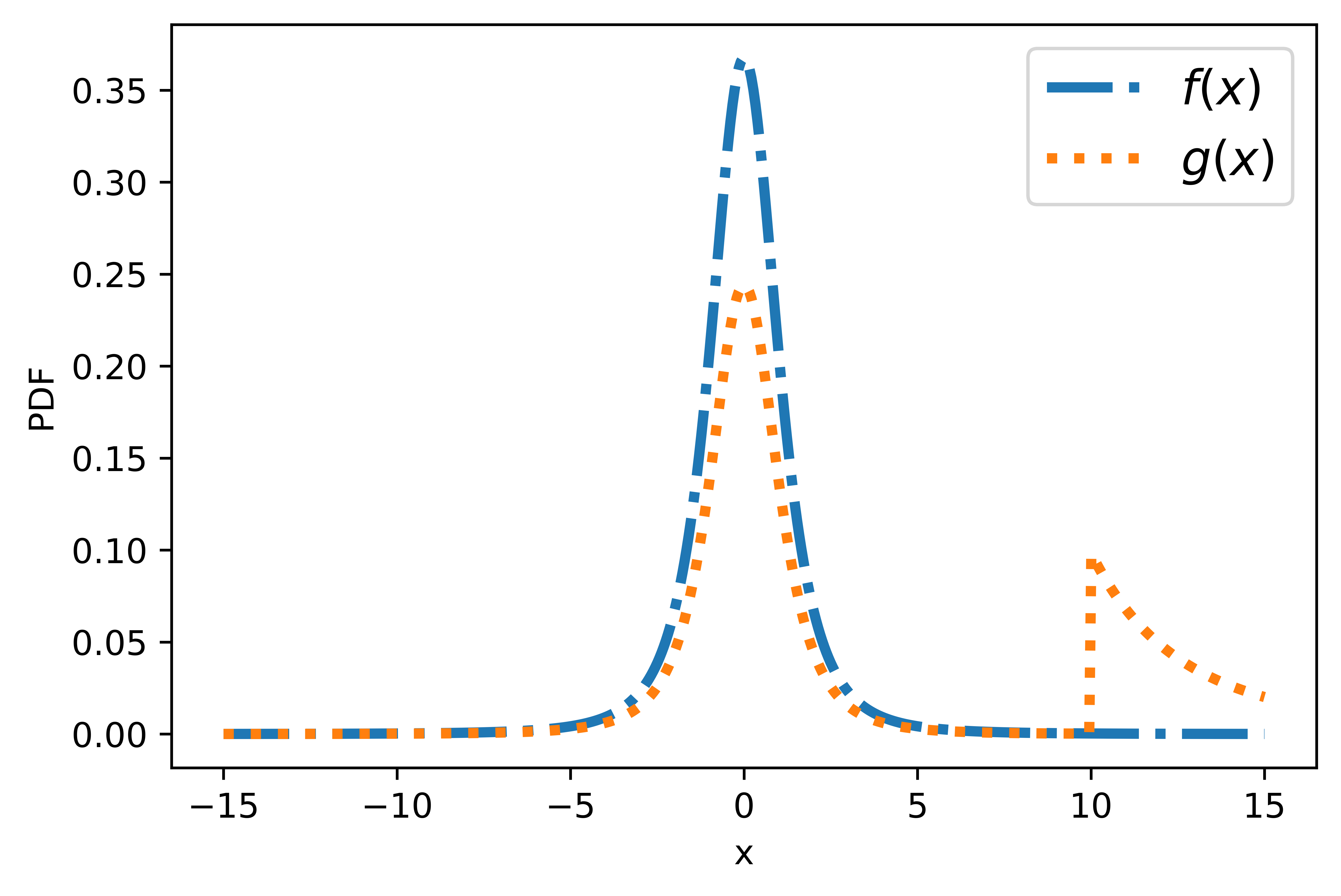
Figure 2: Probability density functions $f$ and $g$ corresponding to the distributions $F$ and $G,$ respectively, as per the construction in the proof of Lemma 3. Here, $F$ is a standard Student’s t-distribution with degrees of freedom parameter 3, and $b=10.$

The KL divergence between $G$ and $F$ is given by

$$\text{KL}(G,F) =\int_{-\infty}^{\infty}\log{\frac{dG(x)}{dF(x)}}dG(x)$$

$$=\int_{-\infty}^{b}\chi_{1}\log{\chi_{1}}dF(x)+\int_{b}^{\infty}b^{p-0.5}\log{b^{p-0.5}}dF(x)$$

$$\leq b^{p-0.5}(p-0.5)\log(b){\overline{F}(b)}\quad(\because\chi_{1}<1).$$

As $\lim_{b\to\infty}b^{p-0.5}\log(b)\overline{F}(b)=0$, we can choose a large enough $b$ such that $\text{KL}(G,F)\leq\delta.$ We further show that as $b$ tends to infinity, the mean and CVaR of $G$ also tend to infinity. This ensures that for a suitably large $b,$ obj(G) can be made greater than $\gamma.$

For $b$ such that $F(b^{+})=F(b^{-}),$

$$\mu(G) =\chi_{1}\int_{-\infty}^{b}xdF(x)+b^{p-0.5}\int_{b}^{\infty}xdF(x)$$

$$\geq\chi_{1}\int_{-\infty}^{b}xdF(x)+b^{p-0.5}\left(b\overline{F}(b)\right).$$

As $\lim_{b\to\infty}b^{p+0.5}\overline{F}(b)=\infty$ and $\lim_{b\to\infty}\chi_{1}\int_{-\infty}^{b}xdF(x)=\mu(F),$ we have $\lim_{b\to\infty}\mu(G)=\infty.$

Similarly, for large enough $b$, $v_{\alpha}(G)=\inf(\xi:\chi_{1}F(\xi)\geq\alpha).$ Also, $\lim_{b\to\infty}v_{\alpha}(G)=v_{\alpha}(F).$ For $b$ large enough such that $F(b^{+})=F(b^{-}),$

$$c_{\alpha}(G)= \frac{1}{1-\alpha}\int_{v_{\alpha}(G)}^{b}\chi_{1}xdF(x)+\frac{1}{1-\alpha}\int_{b}^{\infty}b^{p-0.5}xdF(x)$$

$$\geq \underbrace{\frac{1}{1-\alpha}\int_{v_{\alpha}(G)}^{b}\chi_{1}xdF(x)}_{T_{1}}+\underbrace{\frac{1}{1-\alpha}b^{p+0.5}\overline{F}(b)}_{T_{2}}.$$

Note that $\lim_{b\to\infty}T_{1}=c_{\alpha}(F)$ and $\lim_{b\to\infty}T_{2}=\infty.$ Hence, $\lim_{b\to\infty}c_{\alpha}(G)=\infty.$ ∎

Finally, Theorem 2 is an immediate consequence of Lemmas 2 and 3.

Proof:

As $\nu_{1}$ is regularly varying, $\nu^{\prime}_{1}$ can be chosen so that $KL(\nu^{\prime}_{1},\nu_{1})\leq\delta$ for any small $\delta>0,$ and $\texttt{obj}(\nu_{1}^{\prime})>\texttt{obj}(\nu_{2})>\texttt{obj}(\nu_{1}).$ Considering the alternative instance $\nu^{\prime}=(\nu^{\prime}_{1},\nu_{2}),$ an application of Lemma 2 implies that $c^{*}(\nu)\leq\delta.$ Since $\delta$ can be made arbitrarily small, it follows that $c^{*}(\nu)=0.$ This proves Theorem 2. ∎

IV Statistically robust algorithms

In this section, we propose statistically robust, risk-aware algorithms, and prove performance guarantees for these algorithms. As enforced by the impossibility result proved in Section III, these algorithms produce an (asymptotically) slower-than-exponential decay in the probability of error with respect to the budget $T.$ However, we show that by tuning a certain function that parameterizes the estimators used in these algorithms, the probability of error can be made arbitrarily close to exponentially decaying. In this sense, the class of algorithms proposed are asymptotically near-optimal. This is, however, not an entirely ‘free lunch’—tuning the algorithms to be near-optimal asymptotically (as $T\rightarrow\infty$) leads to a potential degradation of performance for moderate values of $T.$ Interestingly, if noisy prior information is available, say on moment bounds satisfied by the arm distributions, this can be incorporated into our algorithms to improve the short-horizon performance, without affecting their statistical robustness.

This section is organised as follows. We begin by describing the basic framework of the algorithms proposed here. In the following three subsections, different algorithm classes are considered, along with their corresponding performance guarantees. The different algorithm classes differ only in the estimators used for the mean and CVaR of each arm. Indeed, when dealing with heavy-tailed MAB instances, naive estimators based on empirical averages perform poorly (as we demonstrate in Section IV-A), necessitating the use of more sophisticated estimators that are less sensitive to the (relatively frequent) outliers that arise in heavy-tailed data (see Sections IV-B and IV-C).

Our algorithms are of successive rejects (SR) type [37]. They are parameterized by positive integers $n_{1}\leq n_{2}\leq\cdots\leq n_{K-1}$ satisfying $n_{1}=\Omega(T)$ and $\sum_{i=1}^{K-2}n_{i}+2n_{K-1}\leq T.$ The algorithm proceeds in $K-1$ phases, with one arm being rejected from further consideration at the end of each phase. In phase $i,$ the $K+1-i$ arms under consideration are pulled $n_{i}-n_{i-1}$ times, after which the arm with the worst (estimated) performance is rejected. This is formally expressed in Algorithm 1. Here, $\overline{\mu}_{n_{k}}(i)$ and $\overline{c}_{n_{k},\alpha}(i)$ denote generic estimators of the mean and CVaR of arm $i$, respectively, using $n_{k}$ samples from the corresponding distribution. The specific estimators used will differ across the three classes of algorithms we describe later.

Note that the above framework, which we refer to as risk-aware generalized successive rejects, allows for more than one arm elimination at once; for example, if $n_{i}=n_{i+1},$ two arms (the worst performing, among the surviving arms) would in effect be rejected after phase $i.$ Most well known algorithms for fixed budget MABs can be viewed as specific instances of this risk-aware generalized successive rejects framework. For example, the classical SR algorithm in [37] used $n_{k}\propto\frac{T-K}{K+1-k}.$ A related algorithm, called sequential halving (see [41]), eliminates half the surviving arms after each round of pulls (this corresponds to $n_{1}=n_{2}=\cdots=n_{\frac{K}{2}},$ $n_{\frac{K}{2}+1}=n_{\frac{K}{2}+2}=\cdots=n_{\frac{3K}{4}},$ and so on). Another special case is uniform exploration (UE), where $n_{1}=n_{2}=\cdots n_{K-1}=\lfloor T/K\rfloor.$ As the name suggests, under uniform exploration, all arms are pulled an equal number of times, after which the arm with the best estimate is selected.

Algorithm 1 Risk-aware generalized successive rejects algorithm

procedure RA-GSR($T,K,\{n_{1},\cdots,n_{K-1}\}$)

     $A_{1}\leftarrow\{1,\cdots,K\}$

     $n_{0}\leftarrow 0$

     for $k=1\text{ to }K-1$ do

         $\text{For each }i\in A_{k}\text{, pull arm }i\text{ for }n_{k}-n_{k-1}\text{ rounds}$

         $\text{Let }A_{k+1}=A_{k}\setminus\text{arg max}_{i\in A_{k}}\xi_{1}\overline{\mu}_{n_{k}}(i)+\xi_{2}\overline{c}_{n_{k},\alpha}(i)$

     end for

     $\text{Output unique element of }A_{K}$

end procedure

We note here that SR type algorithms require that the budget/horizon $T$ be known a priori. However, if $T$ is not known a priori, any-time variants can be constructed as follows: UE, implemented in a round robin fashion is of course inherently any-time. Risk-aware generalized successive reject algorithms can also be made any-time using the well-known doubling trick (see [42]).

The probability of error of the risk-aware generalized successive rejects algorithm can be upper bounded in the following manner. During phase $k$, at least one of the $k$ worst arms is surviving. Thus, if the optimal arm $i^{*}$ is dismissed at the end of phase $k$, that means:

$$\xi_{1}\overline{\mu}_{n_{k}}(i^{*})+\xi_{2}\overline{c}_{n_{k},\alpha}(i^{*})\geq\\ \min_{i\in\{(K),(K-1),\cdots,(K+1-k)\}}\xi_{1}\overline{\mu}_{n_{k}}[i]+\xi_{2}\overline{c}_{n_{k},\alpha}[i]$$

Using the union bound, we get:

$$\begin{split}p_{e}\leq&\sum_{k=1}^{K-1}\sum_{i=K+1-k}^{K}\mathbb{P}\Big{(}\xi_{1}\overline{\mu}_{n_{k}}(i^{*})+\xi_{2}\overline{c}_{n_{k},\alpha}(i^{*})\\ &\qquad\qquad\qquad\qquad\qquad\geq\xi_{1}\overline{\mu}_{n_{k}}[i]+\xi_{2}\overline{c}_{n_{k},\alpha}[i]\Big{)}\end{split}$$

$$\begin{split}=&\sum_{k=1}^{K-1}\sum_{i=K+1-k}^{K}\mathbb{P}\Big{(}\xi_{1}(\overline{\mu}_{n_{k}}(i^{*})-\mu(i^{*})-(\overline{\mu}_{n_{k}}[i]-\mu[i]))\\ &+\xi_{2}(\overline{c}_{n_{k},\alpha}(i^{*})-c_{\alpha}(i^{*})-(\overline{c}_{n_{k},\alpha}[i]-c_{\alpha}[i]))\geq\Delta[i]\Big{)}\end{split}$$

$$\begin{split}\leq&\sum_{k=1}^{K-1}\sum_{i=K+1-k}^{K}\biggl{(}\mathbb{P}\left(\xi_{1}(\overline{\mu}_{n_{k}}(i^{*})-\mu(i^{*}))\geq\Delta[i]/4\right)\\ &\qquad\qquad\quad+\mathbb{P}\left(\xi_{1}(\mu[i]-\overline{\mu}_{n_{k}}[i])\geq\Delta[i]/4\right)\\ &\qquad\qquad\quad+\mathbb{P}\left(\xi_{2}(\overline{c}_{n_{k},\alpha}(i^{*})-c_{\alpha}(i^{*}))\geq\Delta[i]/4\right)\\ &\qquad\qquad\quad+\mathbb{P}\left(\xi_{2}(c_{\alpha}[i]-\overline{c}_{n_{k},\alpha}[i])\geq\Delta[i]/4\right)\biggr{)}\end{split}$$ (3)

The terms in the summation above can be bounded using suitable concentration inequalities on the estimators $\overline{\mu}_{n}(\cdot)$ and $\overline{c}_{n,\alpha}(\cdot)$—these will be derived for the specific estimators we use in the following subsections.

IV-A Algorithms utilizing empirical average estimators

In this section, we consider the simplest oblivious estimators—those based on empirical averages. Unfortunately, these simple techniques do not enjoy good guarantees; the probability of error decays polynomially (i.e., as a power law) in $T.$ The fundamental reason for this is the poor concentration properties of these estimators when the underlying distribution is heavy-tailed.

We begin by stating the empirical CVaR estimator. We then state our concentration inequality for this CVaR estimator, establish its tightness, and point to analogous existing results for the empirical mean estimator. Finally, we use these inequalities to show that the probability of error of SR-type algorithms using these estimators decays polynomially. This motivates the use of more sophisticated estimators that provide stronger performance guarantees; this is the agenda for the following two subsections.

Suppose that $\{X_{i}\}_{i=1}^{n}$ are $n$ IID samples distributed as the random variable $X.$ Let $\{X_{[i]}\}_{i=1}^{n}$ denote the order statistics of $\{X_{i}\}_{i=1}^{n}$ i.e., $X_{[1]}\geq X_{[2]}\cdots\geq X_{[n]}$. Recall that the classical estimator for $c_{\alpha}(X)$ given the samples $\{X_{i}\}_{i=1}^{n}$ (see [43]) is:

$$\hat{c}_{n,\alpha}(X)=X_{[\lceil n\beta\rceil]}+\frac{1}{n\beta}\sum_{i=1}^{\lfloor n\beta\rfloor}(X_{[i]}-X_{[\lceil n\beta\rceil]}).$$

Now, we state the concentration inequality for $\hat{c}_{n,\alpha}(X)$ when $X$ satisfies C1.

Theorem 3.

Suppose that $\{X_{i}\}_{i=1}^{n}$ are IID samples distributed as $X,$ where $X$ satisfies condition C1. Given $\Delta>0,$

$$\mathbb{P}\left(|\hat{c}_{n,\alpha}(X)-c_{\alpha}(X)|\geq\Delta\right)\leq\frac{C(p,\Delta,V)}{n^{p-1}}+o(\frac{1}{n^{p-1}}),$$

where $C(p,\Delta,V)$ is a positive constant.

The precise statement of the result, with explicit expressions for $C(p,\Delta,V)$ and the $o(\frac{1}{n^{p-1}})$ term above can be found in Appendix B. Note that the upper bound decays polynomially in $n.$ Contrast this with exponentially decaying concentration bounds proved in [44] for bounded random variables (see Lemma 4 below). The bound in Theorem 3 in nearly tight in an order sense, as shown in the following theorem. Similar upper and lower bounds for the concentration of the empirical mean estimator are provided in [2].

Theorem 4.

Suppose that $\{X_{i}\}_{i=1}^{n}$ be IID samples distributed as $X,$ where $X\sim\mathrm{Pareto}(x_{m},a),$ where $x_{m}>0$ and $a>1.$ Then

$$\mathbb{P}(\hat{c}_{n,\alpha}(X)>c_{\alpha}(X)+\Delta)\geq\frac{\beta x_{m}^{a}}{n^{a-1}(c_{\alpha}(X)+\Delta)^{a}}+o\left(\frac{1}{n^{a-1}}\right).$$

The proof of Theorem 4 can be found in Appendix C. If $X\sim\mathrm{Pareto}(x_{m},a),$ then $\mathbb{E}\left[X^{\theta}\right]<\infty$ for $\theta<a$ and $\mathbb{E}\left[X^{\theta}\right]=\infty$ for $\theta\geq a.$ Thus, if $a\in(1,2],$ comparing the upper bound in Theorem 3 to the lower bound in Theorem 4, $p<a$ and $p$ can be made arbitrarily close to $a,$ suggesting the near-tightness of the upper bound of Theorem 3.

Theorem 3 and the analogous result for the empirical mean estimator (see Lemma 3 in [2]), when applied to (3), imply that generalized SR algorithms using empirical average based estimators have a probability of error that is $O(\frac{1}{n^{p-1}}).$ Moreover, Theorem 4 shows that this bound is nearly tight in the order sense. We demonstrate this via the following example.

Corollary 4.1.

Consider a two-arm instance $\nu=(\nu_{1},\nu_{2}).$ Arm 1 is optimal and has a $\mathrm{Pareto}(x_{m},a)$ distribution with $a>1.$ Arm 2 is a constant having a value such that $\texttt{obj}(2)=\texttt{obj}(1)+\Delta.$ The probability of error, $p_{e}$, of any SR-type algorithm using empirical estimators is bounded below by $\frac{C}{T^{a-1}}+o\left(\frac{1}{T^{a-1}}\right),$ where $C>0$ is an instance (and algorithm) dependent constant.

The above corollary is a direct consequence of Theorem 4 and the analogous lower bound for the concentration of the empirical mean from [2]; the proof is omitted.

To summarize, SR algorithms using empirical estimators are statistically robust, but exhibit poor performance, with a probability of error that decays (in the worst case) polynomially with respect to the horizon.

IV-B Algorithms utilizing truncation-based estimators

In this section, we show that SR-type algorithms using truncation-based estimators for the mean and CVaR have considerably stronger performance guarantees compared to the power law bounds seen in Section IV-A. Specifically, we show that by scaling a certain truncation parameter as a suitably slowly growing function of the budget $T,$ the probability of error for these algorithms can be arbitrarily close to exponentially decaying in $T.$

In the following, we first propose a truncation based estimator for CVaR, prove a concentration inequality for same, and finally evaluate the performance of the SR-type algorithms that use these truncation-based estimators.

CVaR Concentration

We begin by stating a concentration inequality for CVaR of bounded random variables from [44].

Lemma 4 (Theorem 3.1 in [44]).

Suppose that $\{X_{i}\}_{i=1}^{n}$ are IID samples distributed as $X,$ where the support of $X,$ $\text{supp}(X)\subseteq[a,b].$ Then, for any $\Delta\geq 0,$

$$\mathbb{P}\left(|\hat{c}_{n,\alpha}(X)-c_{\alpha}(X)|\geq\Delta\right)\leq 6\exp\left(-\frac{1}{11}n\beta\left(\frac{\Delta}{b-a}\right)^{2}\right).$$

We now use Lemma 4 to develop a CVaR concentration inequality for unbounded (potentially heavy-tailed) distributions. In particular, our concentration inequality applies to the following truncation-based estimator. For $b>0,$ define

$$X^{(b)}_{i}=\min(\max(-b,X_{i}),b).$$

Note that $X_{i}^{(b)}$ is simply the projection of $X_{i}$ onto the interval $[-b,b].$ Let $\{X^{(b)}_{[i]}\}_{i=1}^{n}$ denote the order statistics of truncated samples $\{X^{(b)}_{i}\}_{i=1}^{n}.$ Our estimator $\hat{c}_{n,\alpha}^{(b)}(X)$ for $c_{\alpha}(X)$ is simply the empirical CVaR estimator for $X^{(b)}:=\min(\max(-b,X),b),$ i.e.,

$$\hat{c}_{n,\alpha}^{(b)}(X)=\hat{c}_{n,\alpha}(X^{(b)})=X_{[\lceil n\beta\rceil]}^{(b)}+\frac{1}{n\beta}\sum_{i=1}^{\lfloor n\beta\rfloor}(X_{[i]}^{(b)}-X_{[\lceil n\beta\rceil]}^{(b)}).$$ (4)

A truncation-based estimator for the mean is well-known (see [45, 2]); it is given by

$$\hat{\mu}^{\dagger}_{n}(X):=\frac{\sum_{i=1}^{n}X_{j}\mathbbm{1}\left\{|X_{j}|\leq b\right\}}{n}.$$ (5)

Note that the nature of truncation performed for our CVaR estimator is different from that in the truncation-based mean estimator, where samples with an absolute value greater than $b$ are set to zero. In contrast, our estimator projects these samples to the interval $[-b,b].$ This difference plays an important role in establishing the concentration properties of the estimator.

We are now ready to state the concentration inequality for $\hat{c}_{n,\alpha}^{(b)}(X),$ which shows that the estimator works well when the truncation parameter $b$ is large enough.

Theorem 5.

Suppose that $\{X_{i}\}_{i=1}^{n}$ are IID samples distributed as $X,$ where $X$ satisfies condition C1. Given $\Delta>0,$

$$\mathbb{P}\left(|c_{\alpha}(X)-\hat{c}_{n,\alpha}^{(b)}(X)|\geq\Delta\right)\leq 6\text{exp}\bigg{(}-n\beta\frac{\Delta^{2}}{176b^{2}}\bigg{)}$$ (6)

$$\text{ for }b>\max\left(|v_{\alpha}(X)|,\left[\frac{2B}{\Delta\beta}\right]^{\frac{1}{p-1}}\right).$$ (7)

Proof:

We begin by bounding the bias in CVaR resulting from our truncation. It is important to note that so long as $b>|v_{\alpha}(X)|,$ $v_{\alpha}(X)=v_{\alpha}(X^{(b)}).$ Thus, for $b>|v_{\alpha}(X)|,$

$$|c_{\alpha}(X)-c_{\alpha}(X^{(b)})|$$

$$=~{} c_{\alpha}(X)-c_{\alpha}(X^{(b)})$$

$$=~{} \frac{1}{\beta}\bigg{(}\mathbb{E}[X\mathbbm{1}\{X\geq v_{\alpha}(X)\}]-\mathbb{E}[X^{(b)}\mathbbm{1}\{X\geq v_{\alpha}(X)\}]\bigg{)}$$

$$\stackrel{{\scriptstyle(a)}}{{=}}~{} \frac{1}{\beta}\mathbb{E}[(X-b)\mathbbm{1}\{X>b\}]$$

$$\leq~{} \frac{1}{\beta}\mathbb{E}[X\mathbbm{1}\{X>b\}]$$

$$\stackrel{{\scriptstyle(b)}}{{\leq}}~{} \frac{B}{\beta b^{p-1}}.$$ (8)

Here, ($a$) is a consequence of $b>|v_{\alpha}(X)|.$ The bound ($b$) follows from

$$\mathbb{E}[X\mathbbm{1}\{X>b\}]\leq\mathbb{E}\left[\frac{X^{p}}{X^{p-1}}\mathbbm{1}\{X>b\}\right]\\ \leq\frac{1}{b^{p-1}}\mathbb{E}\left[|X|^{p}\right]\leq\frac{B}{b^{p-1}}.$$

It follows from (8) that for $b$ satisfying (7), the bias of our CVaR estimator is bounded as: $|c_{\alpha}(X)-c_{\alpha}(X^{(b)})|\leq\frac{\Delta}{2}.$ Thus, for $b$ satisfying (7), we have

$$\mathbb{P}\left(|c_{\alpha}(X)-\hat{c}_{n,\alpha}^{(b)}(X)|\geq\Delta\right)$$

$$\leq~{} \mathbb{P}\left(|c_{\alpha}(X)-c_{\alpha}(X^{(b)})|+|c_{\alpha}(X^{(b)})-\hat{c}_{n,\alpha}(X^{(b)})|\geq\Delta\right)$$

$$\stackrel{{\scriptstyle(a)}}{{\leq}}~{} \mathbb{P}\left(|c_{\alpha}(X^{(b)})-\hat{c}_{n,\alpha}(X^{(b)})|\geq\frac{\Delta}{2}\right)$$

$$\stackrel{{\scriptstyle(b)}}{{\leq}}~{} 6\text{exp}\bigg{(}-n\beta\frac{(\Delta/b)^{2}}{176}\bigg{)}.$$

Here, ($a$) follows from the bound on $|c_{\alpha}(X)-c_{\alpha}(X^{(b)})|$ obtained earlier. For ($b$), we invoke Lemma 4. ∎

In contrast with the concentration inequality for the empirical CVaR estimator (see Theorem 3), the truncation-based estimator admits an exponential concentration inequality. In other words, the probability of a $\Delta$-deviation between the estimator and the true CVaR decays exponentially in the number of examples, so long as the truncation parameter is set to be large enough.

The key feature of truncation-based estimators like the one proposed here for the CVaR is that they enable a parameterized bias-variance trade-off. While the truncation of the data itself adds a bias to the estimator, the boundedness of the (truncated) data limits the variability of the estimator. Indeed, the condition that $b>\left[\frac{2B}{\Delta\beta}\right]^{\frac{1}{p-1}}$ in the statement of Theorem 5 ensures that the estimator bias induced by the truncation is at most $\Delta/2.$

However, in order to apply the proposed truncation-based estimator in MAB algorithms, one must ensure that for each arm, the truncation parameter satisfies the lower bound (7). This is particularly problematic in the context of statistically robust algorithms, which cannot customize the truncation parameter to work for a narrow class of MAB instances. Our remedy is to set the truncation parameter as an increasing function of the number of data samples $n,$ which ensures that (7) holds for large enough $n.$ Moreover, it is clear from (6) that for the estimation error to (be guaranteed to) decay with $n,$ $b^{2}$ can grow at most linearly in $n.$ Indeed, for our bandit algorithms, we set $b=n^{q},$ where $q\in(0,1/2).$

Finally, we note that it is tempting to set $b$ in a data-driven manner, i.e., to estimate the VaR, moment bounds and so on from the data, and set $b$ large enough so that (7) holds with high probability. The issue however is that $b$ then becomes a (data-dependent) random variable, and proving concentration results with such data-dependent truncation is challenging.

Performance Evaluation

We now evaluate the performance of SR-type algorithms using truncation-based estimators for mean and CVaR. To simplify the presentation, we present the results corresponding to the classical SR algorithm of [37]; here, $n_{k}=\frac{T-K}{(K+1-k)\overline{\log}(K)},$ where $\overline{\log}(K):=1/2+\sum_{i=2}^{K}1/i$. Our results can easily be generalized to other members of the class of risk-aware generalized SR algorithms. We will denote the truncation parameter for the CVaR estimator as $b_{c}$ and the truncation parameter for the mean estimator as $b_{m}.$ Specifically, in phase $k$ of the algorithm, the mean estimator, given by (5), uses the truncation parameter $b_{m}(n_{k})=n_{k}^{q_{m}},q_{m}\in(0,1),$ whereas the CVaR estimator, given by (4), uses truncation parameter $b_{c}(n_{k})=n_{k}^{q_{c}},q_{c}\in(0,0.5).$

Theorem 6.

Let the arms satisfy the condition C1. The probability of incorrect arm identification for the successive rejects algorithm using truncation based estimators is bounded as follows.

$$p_{e}\leq \sum_{i=2}^{K}(K+1-i)2\text{exp}\bigg{(}-\frac{1}{16\xi_{1}}\Big{(}\frac{T-K}{\overline{\log}(K)}\Big{)}^{1-q_{m}}\frac{\Delta[i]}{i^{1-q_{m}}}\bigg{)}$$

$$+ \sum_{i=2}^{K}(K+1-i)6\text{exp}\bigg{(}-\frac{\beta}{2464\xi_{2}^{2}}\Big{(}\frac{T-K}{\overline{\log}(K)}\Big{)}^{1-2q_{c}}\frac{\Delta[i]^{2}}{i^{1-2q_{c}}}\bigg{)}$$

for $T>K+K\overline{\log}(K)n^{*},$ where

$$n^{*} =\max\bigg{(}\Big{(}\frac{12\xi_{1}B}{\Delta[2]}\Big{)}^{\frac{1}{q_{m}\min(p-1,1)}},\Big{(}\frac{8\xi_{2}B}{\beta\Delta[2]}\Big{)}^{\frac{1}{q_{c}(p-1)}},$$

$$\qquad\qquad\qquad\qquad\Big{(}\frac{B}{\text{min}(\alpha,\beta)}\Big{)}^{\frac{1}{q_{c}p}}\bigg{)}.$$

The proof of Theorem 6 can be found in Appendix E. Here, we highlight the main takeaways from this result.

First, note that the probability of error (incorrect arm identification) decays to zero as $T\rightarrow\infty,$ for any instance in $\mathcal{M},$ meaning the proposed algorithm is statistically robust. Moreover, as expected, the decay is slower than exponential in $T;$ taking $q_{m}=q,$ $q_{c}=q/2$ for $q\in(0,1),$ the probability of error is $O(\mathrm{exp}(-\gamma T^{1-q}))$ for an instance dependent positive constant $\gamma.$ Note that this bound on the probability of error is considerably stronger than the power law bounds corresponding to algorithms that use empirical estimators.

Second, our upper bounds only hold when $T$ is larger than a certain instance-dependent threshold. This is because the concentration inequalities on our truncated estimators are only valid when the truncation interval is wide enough (to sufficiently limit the estimator bias). As a consequence, our performance guarantees only kick in once the horizon length is large enough to ensure that this condition is met.

Third, there is a natural tension between the asymptotic behavior of the upper bound for the probability of error and the threshold on $T$ beyond which it is applicable, with respect to the choice of truncation parameters $q_{m}$ and $q_{c}.$ In particular, the upper bound on $p_{e}$ decays fastest with respect to $T$ when $q_{m},q_{c}\approx 0.$ However, choosing $q_{m},q_{c}$ to be small would make the threshold on the horizon to be large, since the bias of our estimators would decay slower with respect to $T.$ Intuitively, smaller values of $q_{m},q_{c}$ limit the variance of our estimators (which is reflected in the bound for $p_{e}$) at the expense of a greater bias (which is reflected in the threshold on $T$), whereas larger values of $q_{m},q_{c}$ limit the bias at the expense of increased variance.

Finally, we note that while the truncation-based SR algorithm as stated is distribution oblivious (i.e., it assumes no prior information about the arm distributions), noisy prior information about the arm distributions can be used to tailor the scaling of the truncation parameters. For example, suppose that it is believed that the MAB instance belongs to $\mathcal{M}(p,B)$ and that the suboptimality gaps are bounded below by $\Delta$ (i.e., $\Delta[2]\geq\Delta$). A natural choice for the truncation parameters would then be

$$b_{m} =\left(\frac{12B\xi_{1}}{\Delta}\right)^{\frac{1}{p-1}}+T^{q},$$

$$b_{c} =\max\left(\left(\frac{B}{\beta}\right)^{\frac{1}{p}},\left[\frac{8B\xi_{2}}{\Delta\beta}\right]^{\frac{1}{p-1}}\right)+T^{q/2},$$

for small $q\in(0,1)$; this would make $n^{*}$ close to zero for instances in $\mathcal{M}(p,B)$ having sub-optimality gaps exceeding $\Delta,$ while ensuring that the probability of error remains $O(\mathrm{exp}(-\gamma T^{1-q}))$ for any instance in $\mathcal{M}.$ Essentially, our prescription on the use of noisy prior information about the arm distributions is to set the truncation parameters as the ‘specialized’ value suggested by the prior information, plus a slowly growing function of the horizon to ensure robustness to the unreliability to the prior information.

IV-C Algorithms utilizing median-of-bins estimators

In this section, inspired by the median-of-means estimator (see [46, 2]), we propose a similar estimator for CVaR and we call it the median-of-cvars estimator. The idea of this estimator is to divide the samples into disjoint bins, compute the empirical CVaR estimator for each bin, and to finally use the median of these estimates. In the following, we first derive a concentration inequality for the median-of-cvars estimator. We then use this result, in conjunction with known concentration properties of the median-of-means estimator, to characterize the performance of SR algorithms that utilise such median-of-bins estimators.

CVaR Concentration

We are now ready the state the first result of this section, which is a concentration inequality for the median-of-cvars estimator.

Theorem 7.

Suppose that $\{X_{i}\}_{i=1}^{n}$ are IID samples distributed as $X,$ where $X$ satisfies condition C1. Divide the sampled into $k$ bins, each containing $N=\lfloor n/k\rfloor$ samples, such that bin $i$ contains the samples $\{X_{j}\}_{j=(i-1)N+1}^{iN}\}.$ Let $\hat{c}_{N,\alpha,i}$ denote the empirical CVaR estimator for the samples in bin $i.$ Let $\hat{c}_{M}$ denote the median of empirical CVaR estimators $\{\hat{c}_{N,\alpha,i}\}_{i=1}^{k}.$ Then given $\Delta>0,$

$$\mathbb{P}\left(|\hat{c}_{M}-c_{\alpha}(X)|\geq\Delta\right)\leq\text{exp}(-\frac{n}{8N})\\$$ (9)

if $N\geq N^{*},$ where $N^{*}$ is a constant that depends on the distribution of $X$ and $\Delta.$

A precise characterization of the constant $N^{*},$ along with the proof of Theorem 7, are provided in Appendix D. Note that like in the case of the truncation-based estimator, the median-of-cvars estimator admits an exponential concentration inequality (so long as the number of samples per bin exceeds the threshold $N^{*}$).

The (distribution dependent) lower bound $N^{*}$ on the number of samples per bin ensures a minimal degree of reliability of the empirical CVaR estimator for each bin. Since we are interested in applying the median-of-cvars estimator in statistically robust algorithms, ensuring that this condition is satisfied for all arms is problematic. As before, our remedy is to set the number of samples per bin as a (slowly) growing function of the horizon $T,$ which ensures that the condition for the CVaR concentration to become meaningful holds so long as the horizon $T$ exceeds an instance-specific threshold.

The median-of-means estimator $\hat{\mu}_{M}$ is computed in a similar fashion, i.e., by taking the median of empirical mean estimators for bins $\{\{X_{j}\}_{j=(i-1)N+1}^{iN}\}_{i=1}^{k}.$ A concentration inequality similar to Theorem 7 can be proved for $\hat{\mu}_{M}$ (see [2] or Appendix F).

Performance Evaluation

As before, for simplicity, we present our results assuming that phase lengths are set as per the SR algorithm of [37]; the generalization to other SR-type algorithms (as described in Algorithm 1) is straightforward. For our statistically robust algorithms, we scale the number of samples per bin as follows. In phase $k$ of successive rejects, we set the number of samples per bin for the CVaR estimator as $N_{c}=n_{k}^{q_{c}},$ where $q_{c}\in(0,1),$ and the number of samples per bin for the mean estimator as $N_{m}=n_{k}^{q_{m}},$ for $q_{m}\in(0,1).$ We now state the upper bound on the probability of error for this algorithm.

Theorem 8.

Let the arms satisfy the condition C1. The probability of incorrect arm identification for the successive rejects algorithm using median-of-bins estimators is bounded as follows

$$p_{e}\leq\sum_{k=1}^{K-1}k\Bigg{[}\exp\left(-\frac{1}{8}\left(\frac{T-K}{\overline{\log}(K)(K+1-k)}\right)^{1-q_{m}}\right)\\ +\exp\left(-\frac{1}{8}\left(\frac{T-K}{\overline{\log}(K)(K+1-k)}\right)^{1-q_{c}}\right)\Bigg{]}$$

for $T>T^{*},$ where $T^{*}$ is a instance-dependent threshold.

The explicit expression for $T^{*}$ and the proof of the theorem can be found in Appendix F. In the following, we highlight the key takeaways from Theorem 8.

First, SR algorithms based on median-of-bins estimators are statistically robust, like their truncation-based counterparts. Indeed, setting $q_{c}=q_{m}=q,$ the probability of error is $O(\mathrm{exp}(-\gamma T^{1-q}))$ for any instance in $\mathcal{M},$ where $\gamma$ is a positive instance-dependent constant. In other words, the probablity of error decays sub-exponentially, but much faster than the power law decay arising from the use of empirical averages.

Second, our performance guarantee only hold when $T$ is large enough. As with the truncation-based approach, this is because favourable concentration properties of the median-of-bins estimators only apply when the horizon is large enough.

Third, there is again a tension between the bound on the probability of error and the threshold on $T$ beyond which the bounds are applicable, with respect to the choice of $q_{m}$ and $q_{c}$. To get the best asymptotic upper bound, $q_{m}$ and $q_{c}$ should be close to zero, but this would make $T^{*}$ large, affecting the the short-horizon performance.

Finally, we note that the SR algorithm using median-of-bins estimators as stated is also distribution oblivious. However, as with the truncation-based approach, noisy prior information about the instance can be used to tailor the scaling of the bin sizes for mean and CVaR estimation to improve the short-horizon performance. For example, if it is believed that the MAB instance belongs to $\mathcal{M}(p,B,V)$ and the suboptimality gaps are bounded below by $\Delta,$ the mean and CVaR bin sizes may be chosen as follows:

$$N_{m} =\frac{576\xi_{1}V}{\Delta}+T^{q},$$

$$N_{c} =N^{*}+T^{q},$$

where $q\in(0,1)$ is small and $N^{*}$ is a constant that depends on $(p,B,V,\Delta,\xi_{2})$ (see Appendix D for details). This choice would make $T^{*}$ close to zero for instances that lie in the sub-class under consideration, without affecting the overall statistical robustness of the algorithm. As before, this choice boils down to the ‘specialized’ choice of bin size dictated by the moment bounds, plus a slowly growing function of the horizon for robustness.

V Numerical Experiments

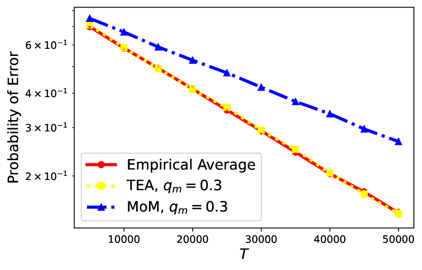
(a) Mean Minimization

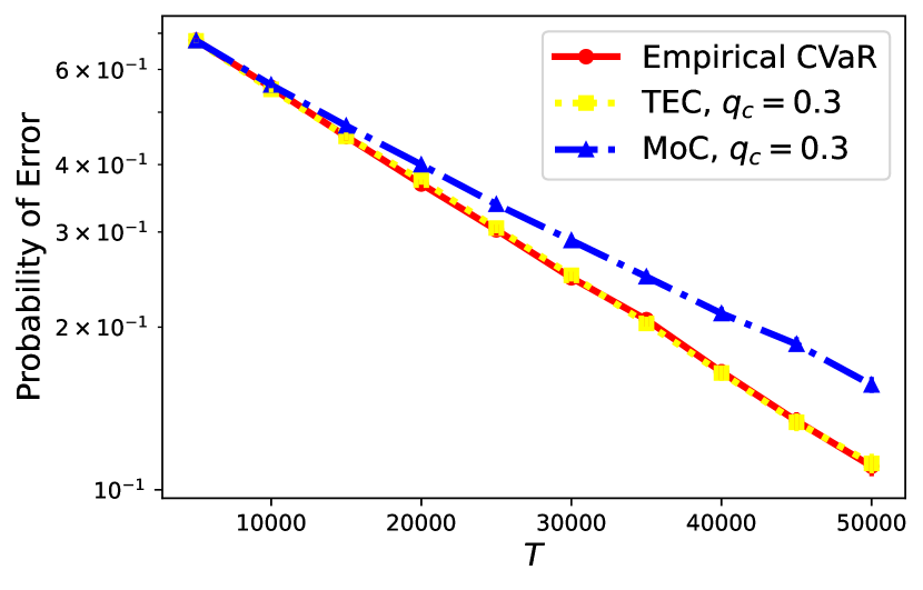
(b) CVaR Minimization

Figure 3: Exponentially Distributed Arms

In this section, we evaluate the performance of the three statistically robust algorithm classes presented in the previous section. We also provide an example to demonstrate the fragility of ’specialized’ algorithms based on noisy prior information. We restrict ourselves to the classical successive rejects (SR) sizing of phases, and primarily focus on two specific objectives: (i) mean minimization, i.e., $(\xi_{1},\xi_{2})=(1,0),$ and (ii) CVaR minimization, i.e., $(\xi_{1},\xi_{2})=(0,1).$ At the end of this section, we also demonstrate the performance of our algorithms on two instances where the objective is a non-trivial convex combination of mean and CVaR. In all the experiments below, CVaR is calculated at a confidence level $\alpha$ of 0.95. Moreover, in each of the experiments below, the probability of error is computed by averaging over 50000 runs at each value of $T$. Confidence intervals for probability of error are calculated at a confidence of $99.9\%.$ As the number of runs is quite large, the confidence intervals are not visible unless the probabilities are very small.

Light-tailed arms: Consider the case when all the arms are light-tailed. In particular, for mean minimization we consider the following MAB problem instance: there are 10 arms, exponentially distributed, the optimal having mean loss 0.97, and the remaining having mean loss 1. For CVaR minimization, consider the following MAB problem instance: there are 10 arms, exponentially distributed, the optimal having a CVaR 2.85, and the remaining having a CVaR 3.00. Parameters $q_{m}$ and $q_{c}$ for the truncation estimators (see Section IV-B) are set to 0.3. Parameters $q_{m}$ and $q_{c}$ for the median-of-bins estimators (see Section IV-C) are also set to 0.3.

As can be seen in Figure 3(a) and Figure 3(b), the truncation-based algorithms and the algorithms using empirical averages perform comparably well, whereas median-of-bins algorithms produce an inferior performance. Because the arm distributions have limited variability in this example, the truncation-based estimators introduce very little bias, and are nearly indistinguishable from the estimators based on empirical averages. On the other hand, the median-of-bins estimators suffer from the poorer concentration of the empirical averages per bin, which is not sufficiently compensated by computing the median across bins.

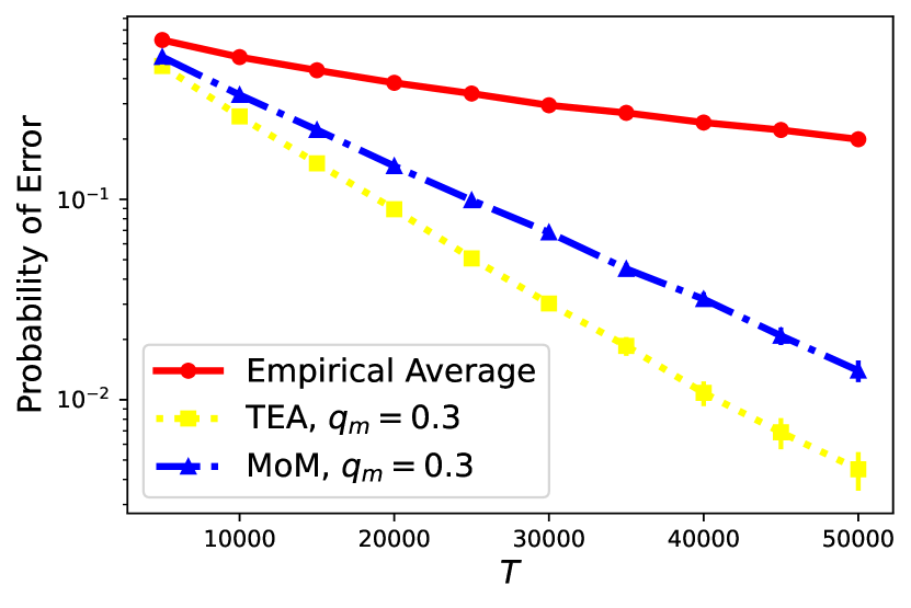
(a) Mean Minimization

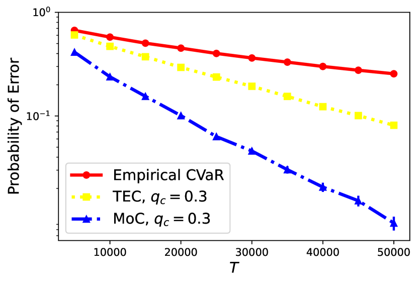
(b) CVaR Minimization

Figure 4: Lomax Distributed Arms

Heavy-tailed arms: Next, consider the case when all the arms are heavy-tailed. For mean minimization we consider the following MAB problem instance: there are 10 arms, distributed according to the lomax distribution (shape parameter = 1.8), the optimal arm having mean loss 0.9, and the remaining arms having mean loss 1. For CVaR minimization, consider the following MAB problem instance: there are 10 arms, distributed according to lomax distribution (shape parameter = 2.0), the optimal having a CVaR 2.55, and the remaining having a CVaR 3.00. Note that like the previous case, parameters $q_{m}$ and $q_{c}$ for the truncation estimators are set to 0.3 and parameters $q_{m}$ and $q_{c}$ for the median-of-bins estimators are also set to 0.3 (see Sections IV-B, IV-C).

As can be seen in Figure 4(a) and Figure 4(b), the algorithms using empirical estimators have a markedly inferior performance compared to the truncation-based and algorithms based on median-of-bins. This is to be expected, since the latter approaches are more robust to the outliers inherent in heavy-tailed data.

Fragility of specialized algorithms: Finally, we present an example where specialized algorithms using noisy information perform poorly, but our robust algorithms perform very well. We consider the problem of CVaR minimization on the following instance involving both heavy-tailed as well as light-tailed arms: there are 10 arms, five distributed according to a lomax distribution (shape parameter=2.0; and the CVaR=3.00), and five distributed exponentially, the optimal arm having a CVaR 2.55, and the remaining four arms having a CVaR 3.00. As before, we set the confidence value to be 0.95. What makes this instance (with a light-tailed optimal arm) challenging is that the bias of truncation-based estimators can result in a significant under-estimation of the CVaR for heavy-tailed arms, causing our algorithms to erroneously declare one of the heavy-tailed arms as optimal.

On this instance, we compare the performance of the following algorithms. Our first candidate is a specialized algorithm that has access to valid bounds pertaining to the instance. In particular, it knows $p=1.9,$ $B=0.057,$ and $\Delta=0.45.$ It uses truncated empirical CVaR as an estimator with truncation parameter being equal to $(\nicefrac{{4B}}{{\beta\Delta}})^{\nicefrac{{1}}{{p-1}}}.$ Our second candidate is another specialized algorithm, but having the following noisy information, $\hat{p}=2,$ $\hat{B}=0.05,$ and $\hat{\Delta}=0.6.$ Note that the parameters have been very slightly perturbed. This algorithm also uses the truncated empirical CVaR as an estimator with truncation parameter being equal to $(\nicefrac{{4\hat{B}}}{{\beta\hat{\Delta}}})^{\nicefrac{{1}}{{\hat{p}-1}}}.$ Our final candidate is a robust algorithm which also has access to the noisy parameters as stated above but it sets the truncation parameter as $(\nicefrac{{4\hat{B}}}{{\beta\hat{\Delta}}})^{\nicefrac{{1}}{{\hat{p}-1}}}+T^{0.3}.$ As can be seen in Figure 5, algorithm with noisy estimates performs very poorly but our robust algorithm performs nearly as good as the non-oblivious algorithm.

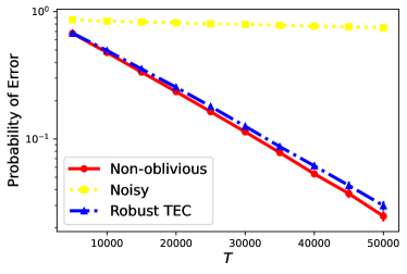
Figure 5: Robustness against noisy parameters

Optimizing a non-trivial combination of mean and CVaR: We now present two instances where the objectives are non-trivial convex combinations of mean and CVaR. We focus on comparing the algorithm based on empirical estimators with algoritms based on the truncation-based estimators. In the first instance, we compare the performance in a reward-seeking setting, i.e., having a lower mean (loss) is preferred over having a lower CVaR. In the second instance, we compare the algorithms in a risk-averse setting, i.e., having a lower CVaR is preferred to having a lower mean.

For the first instance, we set the weight for the mean of an arm, $\xi_{1}$ to be equal to 0.9, and we set the weight for the CVaR of an arm, $\xi_{2}$ to be equal to 0.1. The optimal arm is Lomax distributed with mean equal to 0.85, the shape parameter equal to 2, and the CVaR is approximately 6.75. The non-optimal arms are also Lomax distributed with their means equal to 1, the shape parameters equal to 2.75, and the CVaR is approximately 6.42. Notice that the optimal arm has a smaller mean (loss) but a larger CVaR when compared to the non-optimal arms. Also, notice that the optimal arm is more heavy-tailed than the non-optimal arms, owing to the smaller shape parameter.

For the second instance, we set the weight for the mean of an arm, $\xi_{1}$ to be equal to 0.1, and we set the weight for the CVaR of an arm, $\xi_{2}$ to be equal to 0.9. The optimal arm is again Lomax distributed with CVaR equal to 2.55, the shape parameter equal to 2.75, and the mean is approximately 0.40. The non-optimal arms are also Lomax distributed with CVaR equal to 3, the shape parameter equal to 2, and the mean is approximately 0.38. Notice that the optimal arm has a smaller CVaR but a larger mean compared to the non-optimal arms. Also, notice that the optimal arm is less heavy-tailed than the non-optimal arms, owing to the larger shape parameter.

The peformance is plotted in Figures 6(a) and 6(b). We can observe that slower truncation growth leads to a good performance in the first instance but leads to a worse performance in the second instance. The bias of the truncation based estimators could lead to significant underestimation of the objective for more heavy-tailed arms. This is helpful in the first instance where the optimal arm is more heavy-tailed than the non-optimal arms, but it is problematic in the second instance where the optimal arm is less heavy-tailed than the non-optimal arms. The behaviour of algorithms based on median-of-bins is qualitatively similar to the truncation-based algorithms but the above effect is much more pronounced. In particular, the performance in the first instance is exceptionally good but the performance in the second instance is quite poor. Overall, we observe that truncation-based algorithms are more stable than median-of-bins-based algorithms, although the growth of truncation parameters requires careful tuning.

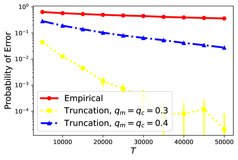
(a) $\xi_{1}=0.9,~{}\xi_{2}=0.1$

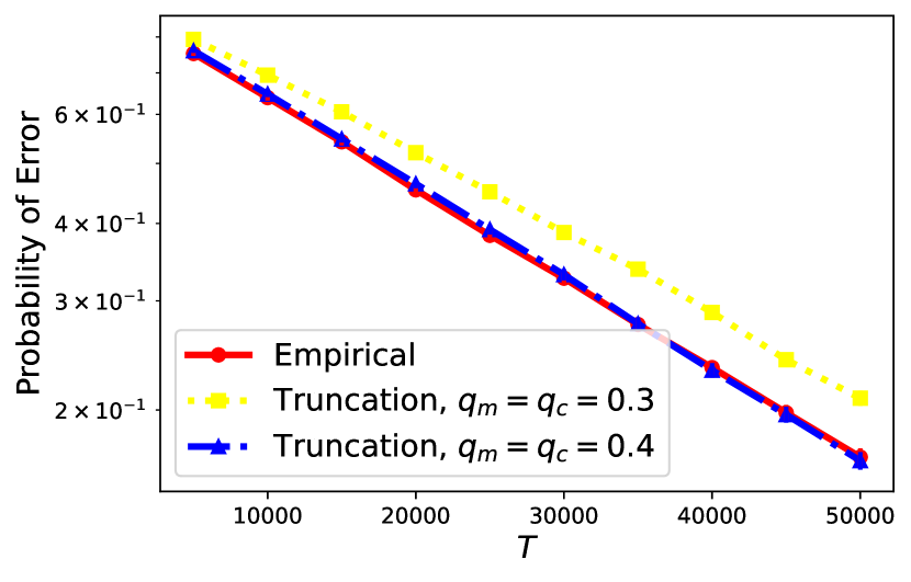
(b) $\xi_{1}=0.1,~{}\xi_{2}=0.9$

Figure 6: Non-trivial combination of mean & CVaR

VI Concluding Remarks

In this paper, we considered the problem of risk-aware best arm selection in a pure exploration MAB framework. Our results highlight the fragility of existing MAB algorithms that require reliable moment/tail bounds to provide strong performance guarantees. We established fundamental performance limits of statistically robust MAB algorithms under fixed budget. We then design algorithms that are statistically robust to parameter misspecification. Specifically, we propose distribution oblivious algorithms, i.e., those that do not need any information on the underlying arms’ distributions. The proposed algorithms leverage ideas from robust statistics and enjoy near-optimal performance guarantees.

The paper motivates future work along several directions. First, it would be interesting to design statistically robust variants of the (stronger) concentration inequalities developed recently for CVaR and mean in [21] and [47] and apply those to the MAB problem considered here. Second, it is not always clear which linear combination of mean and CVaR should be defined as the arm objective in our MAB formulation, given that this involves expressing the mean cost/reward of an arm and the associated risk on the same scale. This motivates the analysis of risk-constrained MAB formulations, where the optimal arm is defined as the one with optimizes the mean cost/reward, subject to a risk constraint.

Appendix A Proof of Theorem 1

The proof is an easy application of Lemma 2 which we will state here again for easy reference.
Let $\nu=(\nu_{1},\nu_{2})$ be a two-armed bandit model such that $\xi_{1}\mu(1)+\xi_{2}c_{\alpha}(1)<\xi_{1}\mu(2)+\xi_{2}c_{\alpha}(2)$ for given $\xi_{1},\xi_{2}\geq 0.$ Any consistent algorithm satisfies

$$\limsup_{t\to\infty}-\frac{1}{t}\log p_{e}(\nu,t)\leq c^{*}(\nu),$$ (10)

where,

$$c^{*}(\nu):=\inf_{(\nu_{1}^{\prime},\nu_{2}^{\prime})\in\mathcal{M}:\texttt{obj}^{\prime}(1)>\texttt{obj}^{\prime}(2)}\max(\text{KL}(\nu_{1}^{\prime},\nu_{1}),\text{KL}(\nu_{2}^{\prime},\nu_{2}))$$

By taking $(\nu_{1}^{\prime},\nu_{2}^{\prime})=(\nu_{2},\nu_{1}),$ we get a trivial upper bound on $c^{*}(\nu),$ i.e., $c^{*}(\nu)\leq\max(\text{KL}(\nu_{2},\nu_{1}),\text{KL}(\nu_{1},\nu_{2})).$ This proves Theorem 1.

Appendix B Proof of Theorem 3

Theorem 9.

Suppose that $\{X_{i}\}_{i=1}^{n}$ are IID samples distributed as $X,$ where $X$ satisfies condition C1. For $p\in(1,2],$ given $\Delta>0$,

$$\begin{aligned} &\mathbb{P}(\hat{c}_{n,\alpha}(X)\leq c_{\alpha}(X)-\Delta)\leq~{}\frac{180{V_{\text{emp}}}}{(n\beta)^{p-1}\Delta^{p}}\\ &\qquad\qquad\qquad+\text{exp}\Big{(}-\frac{n\beta}{8}\min\Big{(}1,\frac{\Delta^{2}\beta^{2/p}}{B^{2/p}}\Big{)}\Big{)}\end{aligned}$$ (11a)

$$\begin{aligned} &\mathbb{P}(\hat{c}_{n,\alpha}(X)\geq c_{\alpha}(X)+\Delta)\leq~{}\frac{360{V_{\text{emp}}}}{(n\beta)^{p-1}\Delta^{p}}+\frac{72{V_{\text{emp}}}\beta}{(n\beta)^{p-1}B}\\ &\qquad+\text{exp}\Big{(}-\frac{n\beta^{1+2/p}\Delta^{2}}{8B^{2/p}+2\Delta(B\beta)^{1/p}}\Big{)}+\text{exp}\Big{(}-\frac{n\beta}{8}\Big{)}\end{aligned}$$ (11b)

$$\begin{aligned} \text{where }{V_{\text{emp}}}=\frac{2^{p-1}V}{\beta}+2^{p}\frac{B}{\beta}.\end{aligned}$$ (11c)

We will first state three lemmas that will be used repeatedly for proving Theorem 9. We begin by stating a concentration inequality for empirical average (see Lemma 2, [3]) .

Lemma 5.

Let $X$ be a random variable satisfying C1. Let $\hat{\mu}_{n}$ be the empirical mean, then for any $\Delta>0$ we have:

$$\mathbb{P}(|\hat{\mu}_{n}-\mu|>\Delta)\leq\begin{cases}\frac{C_{p}V}{n^{p-1}\Delta^{p}}&\text{for }1<p\leq 2\\ \frac{C_{p}V}{n^{p/2}\Delta^{p}}&\text{for }p>2\end{cases}$$

where $C_{p}=(3\sqrt{2})^{p}p^{p/2}.$

Next, consider the inequalities bounding the empirical CVaR estimator (see Lemma 3.1, [44]).

Lemma 6.

Let $X_{[i]}$ be the decreasing order statistics of $X_{i}$; then $f(k)=\frac{1}{k}\sum_{i=1}^{k}X_{[i]},~{}1\leq k\leq n$, is decreasing and the following two inequalities hold:

$$\frac{1}{n\beta}\sum_{i=1}^{\lfloor n\beta\rfloor}X_{[i]} \leq\hat{c}_{n,\alpha}(X)\leq\frac{1}{n\beta}\sum_{i=1}^{\lceil n\beta\rceil}X_{[i]}$$ (12a)

$$f(\lceil n\beta\rceil) \leq\hat{c}_{n,\alpha}(X)\leq f(\lfloor n\beta\rfloor)$$ (12b)

We also state the Chernoff Bound for Bernoulli experiments.

Lemma 7.

Let $Y_{1},...,Y_{n}$ be independent Bernoulli experiments, $\mathbb{P}(Y_{i}=1)=p_{i}$. Set $S=\sum_{i=1}^{n}Y_{i}$, $\mu=\mathbb{E}[Y]$. Then for every $0<\delta<1$,

$$P(S\leq(1-\delta)\mu)\leq\text{exp}(-\frac{\mu\delta^{2}}{2}),$$

for every $\delta>0$,

$$P(S\geq(1+\delta)\mu)\leq\text{exp}(-\frac{\mu\delta^{2}}{2+\delta}).$$

Now, we upper bound the CVaR and mean in terms of parameters $B,$ $p,$ and $\beta.$

$$c_{\alpha}(X)=~{} \frac{1}{\beta}\mathbb{E}\left[X\mathbbm{1}\left\{X\geq v_{\alpha}(X)\right\}\right]$$

$$=~{} \frac{1}{\beta}\int_{v_{\alpha}(X)}^{\infty}xdF_{X}(x)$$

$$\leq~{} \int_{v_{\alpha}(X)}^{\infty}|x|\frac{dF_{X}(x)}{\beta}$$

$$\leq~{} \Big{(}\int_{v_{\alpha}(X)}^{\infty}|x|^{p}\frac{dF_{X}(x)}{\beta}\Big{)}^{\frac{1}{p}}~{}(\text{Using Jensen's Inequality})$$

$$\leq~{} \Big{(}\int_{-\infty}^{\infty}|x|^{p}\frac{dF_{X}(x)}{\beta}\Big{)}^{\frac{1}{p}}$$

$$\leq~{} \Big{(}\frac{B}{\beta}\Big{)}^{\frac{1}{p}}~{}(\text{Using bound on }p^{th}\text{ moment})$$

Similarly, we can show

$$\mathbb{E}\left[|X|\right]\leq\Big{(}\frac{B}{\beta}\Big{)}^{\frac{1}{p}}.$$

Hence,

$$c_{\alpha}(X)\leq\Big{(}\frac{B}{\beta}\Big{)}^{\frac{1}{p}}$$ (13)

$$\mathbb{E}\left[|X|\right]\leq\Big{(}\frac{B}{\beta}\Big{)}^{\frac{1}{p}}$$ (14)

Now, consider the random variable $\tilde{X}$ which is distributed according to $\mathbb{P}(X\in\cdot~{}|X\in[v_{\alpha}(X),\infty))$. Note that $\mathbb{E}\left[\tilde{X}\right]=c_{\alpha}(X)$ and $dF_{\tilde{X}}(x)=\frac{dF_{X}(x)}{\beta}$. Let us find a bound on $\mathbb{E}\left[|\tilde{X}-c_{\alpha}(X)|^{p}\right]$.

$$\mathbb{E}\left[|\tilde{X}-c_{\alpha}(X)|^{p}\right]=\int_{v_{\alpha}(X)}^{\infty}|x-c_{\alpha}(X)|^{p}\frac{dF_{X}(x)}{\beta}$$

$$\begin{split}&\leq\int_{v_{\alpha}(X)}^{\infty}2^{p-1}(|x-\mu|^{p}+|c_{\alpha}(X)-\mu|^{p})\frac{dF_{X}(x)}{\beta}\\ &\qquad\qquad\qquad\qquad\qquad\qquad(\text{Using Jensen's Inequality})\end{split}$$

$$\leq\frac{2^{p-1}V}{\beta}+2^{p-1}(c_{\alpha}(X)-\mu)^{p}$$

$$\leq\frac{2^{p-1}V}{\beta}+2^{p}\frac{B}{\beta}={V_{\text{emp}}}\quad(\text{Using }\ref{eq:cvar-mag-bound},~{}\ref{eq:mean-mag-bound},\text{ and }\ref{eq:bound_vhat})$$

Hence,

$$\mathbb{E}\left[|\tilde{X}-c_{\alpha}(X)|^{p}\right]\leq{V_{\text{emp}}}$$ (15)

B-A Proof of 11a

Let $X_{[i]}$ be the decreasing order statistics of $X_{i}$. We’ll condition the probability above on a random variable $K_{n,\beta}$ which is defined as $K_{n,\beta}$ = max$\{i:X_{[i]}\in[v_{\alpha}(X),\infty)\}$. Note that $v_{\alpha}(X)$ is a constant such that the probability of a $X$ being greater than $v_{\alpha}(X)$ is $\beta$. Also observe that $\mathbb{P}(K_{n,\beta}=k)=\mathbb{P}(k$ from $\{X_{i}\}_{i=1}^{n}$ have values in $[v_{\alpha}(X),\infty))$. Using the above two statements one can easily see that $K_{n,\beta}$ follows a binomial distribution with parameters $n$ and $\beta$. For ease of notation, we let $p^{\prime}:=\min(p/2,p-1)$.

Consider $k$ IID random variables $\{\tilde{X}_{i}\}_{i=1}^{k}$ which are distributed according to $\mathbb{P}(X\in\cdot~{}|X\in[v_{\alpha}(X),\infty))$. By conditioning on $K_{n,\beta}=k$, one can observe using symmetry that $\frac{1}{k}\sum_{i=1}^{k}X_{[i]}$ and $\frac{1}{k}\sum_{i=1}^{k}\tilde{X}_{i}$ have the same distribution. We’ll next bound the probability $\mathbb{P}(\hat{c}_{n,\alpha}(X)\leq c_{\alpha}(X)-\Delta|K_{n,\beta}=k)$ for different values of $k$. Now,

$$\mathbb{P}(\hat{c}_{n,\alpha}(X)\leq c_{\alpha}(X)-\Delta)$$

$$= \sum_{k=0}^{n}\mathbb{P}(K_{n,\beta}=k)\mathbb{P}(A)$$

$$\leq \underbrace{\sum_{k=0}^{\lfloor n\beta\rfloor}\mathbb{P}(K_{n,\beta}=k)\mathbb{P}(A)}_{I_{2}}+\underbrace{\sum_{k=\lceil n\beta\rceil}^{n}\mathbb{P}(K_{n,\beta}=k)\mathbb{P}(A)}_{I_{1}}$$

where $\mathbb{P}(A)=\mathbb{P}(\hat{c}_{n,\alpha}(X)\leq c_{\alpha}(X)-\Delta|K_{n,\beta}=k)$.

Bounding $I_{1}$

Note that $k\geq\lceil n\beta\rceil$. We’ll begin by bounding $P(A)$.

$$\mathbb{P}(\hat{c}_{n,\alpha}(X)\leq c_{\alpha}(X)-\Delta|K_{n,\beta}=k)$$

$$\leq~{} \mathbb{P}\bigg{(}\frac{1}{\lceil n\beta\rceil}\sum_{i=1}^{\lceil n\beta\rceil}X_{[i]}\leq c_{\alpha}(X)-\Delta|K_{n,\beta}=k\bigg{)}~{}(\text{using \ref{eq:wang-b}})$$

$$\begin{split}\leq~{}&\mathbb{P}\bigg{(}\frac{1}{k}\sum_{i=1}^{k}X_{[i]}\leq c_{\alpha}(X)-\Delta|K_{n,\beta}=k\bigg{)}\\ &\qquad\qquad\qquad\qquad\qquad\qquad\qquad(\because f(\cdot)\text{ is decreasing})\end{split}$$

$$=~{} \mathbb{P}\bigg{(}\frac{1}{k}\sum_{i=1}^{k}\tilde{X}_{i}\leq c_{\alpha}(X)-\Delta\bigg{)}$$

$$\begin{split}\leq~{}&\frac{C_{p}{V_{\text{emp}}}}{k^{p^{\prime}}\Delta^{p}}\quad(\text{Using Lemma~{}\ref{ea-conc-lemma} \& \eqref{eq:cvar-centred-bound} and }p^{\prime}=\min(p-1,p/2))\\ \end{split}$$

Hence, we have the following:

$$I_{1}=~{} \sum_{k=\lceil n\beta\rceil}^{n}\binom{n}{k}\beta^{k}(1-\beta)^{n-k}\mathbb{P}(A)$$

$$\leq~{} \sum_{k=\lceil n\beta\rceil}^{n}\binom{n}{k}\beta^{k}(1-\beta)^{n-k}\frac{C_{p}{V_{\text{emp}}}}{k^{p^{\prime}}\Delta^{p}}$$

$$\leq~{} \frac{C_{p}{V_{\text{emp}}}}{(n\beta)^{p^{\prime}}\Delta^{p}}$$

Bounding $I_{2}$

Note that $k\leq\lfloor n\beta\rfloor$. We’ll again start by bounding $\mathbb{P}(A)$. For simplicity of notation, we’ll denote the $\Big{(}\frac{B}{\beta}\Big{)}^{\frac{1}{p}}$ as $b$. Hence, we have $c_{\alpha}(X)\leq b$ as shown in 13.

$$\mathbb{P}(\hat{c}_{n,\alpha}(X)\leq c_{\alpha}(X)-\Delta|K_{n,\beta}=k)$$

$$\leq~{} \mathbb{P}\Big{(}\frac{1}{n\beta}\sum_{i=1}^{\lfloor n\beta\rfloor}X_{[i]}\leq c_{\alpha}(X)-\Delta\Big{|}K_{n,\beta}=k\Big{)}~{}(\text{Using \ref{eq:wang-a}})$$

$$\begin{split}\leq~{}&\mathbb{P}\Big{(}\frac{1}{k}\sum_{i=1}^{k}X_{[i]}\leq\frac{n\beta}{k}(c_{\alpha}(X)-\Delta)\Big{|}K_{n,\beta}=k\Big{)}\\ &\qquad\qquad\qquad\qquad\qquad\qquad\qquad\qquad(\because~{}k\leq\lfloor n\beta\rfloor)\end{split}$$

$$\begin{split}\leq~{}&\mathbb{P}\bigg{(}\frac{1}{k}\sum_{i=1}^{k}X_{[i]}\leq c_{\alpha}(X)+\Big{(}\frac{n\beta}{k}-1\Big{)}b-\frac{n\beta\Delta}{k}\Big{|}K_{n,\beta}=k\bigg{)}\\ &\qquad\qquad\qquad\qquad\qquad\qquad\qquad\qquad(\because c_{\alpha}(X)\leq b)\end{split}$$

Case 1 $\Delta\in[b,\infty)$

Let $\Delta_{1}(k)=\frac{n\beta\Delta}{k}+\Big{(}1-\frac{n\beta}{k}\Big{)}b=b\bigg{(}1+\Big{(}\frac{\Delta}{b}-1\Big{)}\frac{n\beta}{k}\bigg{)}$. Note that $\Delta_{1}(k)>0$ for all $k$ as $\Delta\geq b$. Also note that $\Delta_{1}(k)$ decreases as $k$ increases. As $k\leq n\beta$, $\Delta_{1}(k)\geq\Delta$.

$$\mathbb{P}\Big{(}\frac{1}{k}\sum_{i=1}^{k}X_{[i]}\leq c_{\alpha}(X)-\Delta_{1}(k)|K_{n,\beta}=k\Big{)}$$

$$=~{} \mathbb{P}\Big{(}\frac{1}{k}\sum_{i=1}^{k}\tilde{X}_{i}\leq c_{\alpha}(X)-\Delta_{1}(k)\Big{)}$$

$$\leq~{} \frac{C_{p}{V_{\text{emp}}}}{k^{p^{\prime}}\Delta_{1}^{p}(k)}$$

$$\leq~{} \frac{C_{p}{V_{\text{emp}}}}{k^{p^{\prime}}\Delta^{p}}$$

Now, let us bound $I_{2}$.

$$I_{2}=~{} \sum_{k=0}^{\lfloor n\beta\rfloor}\binom{n}{k}\beta^{k}(1-\beta)^{n-k}\mathbb{P}(A)$$

$$\begin{split}\leq~{}&\sum_{k=0}^{\lfloor n\beta/2\rfloor}\binom{n}{k}\beta^{k}(1-\beta)^{n-k}\\ &+\sum_{k=\lceil n\beta/2\rceil}^{\lfloor n\beta\rfloor}\binom{n}{k}\beta^{k}(1-\beta)^{n-k}\frac{C_{p}{V_{\text{emp}}}}{k^{p^{\prime}}\Delta^{p}}\end{split}$$

$$\leq~{} \mathbb{P}(K_{n,\beta}\leq\lfloor n\beta/2\rfloor)+\frac{2^{p^{\prime}}C_{p}{V_{\text{emp}}}}{(n\beta)^{p^{\prime}}\Delta^{p}}$$

$$\leq~{} \frac{2^{p^{\prime}}C_{p}{V_{\text{emp}}}}{(n\beta)^{p^{\prime}}\Delta^{p}}+e^{-n\beta/8}\quad(\text{Using Chernoff on }K_{n,\beta})$$

Case 2 $\Delta\in(0,b)$

Here, $\Delta_{1}(k)=\frac{n\beta\Delta}{k}-\Big{(}\frac{n\beta}{k}-1\Big{)}b=b\bigg{(}1-\Big{(}1-\frac{\Delta}{b}\Big{)}\frac{n\beta}{k}\bigg{)}$. Note that $\Delta_{1}(k)>0$ iff $k>n\beta(1-\frac{\Delta}{b})$.

Case 2.1 If $\Delta$ is very small such that $\lfloor n\beta\rfloor\leq n\beta\Big{(}1-\frac{\Delta}{b}\Big{)}$, then $\Delta_{1}(k)\leq 0$. Let’s bound $I_{2}$ for this case:

$$I_{2} \leq\sum_{k=0}^{\lfloor n\beta\rfloor}\mathbb{P}(K_{n,\beta}=k)$$

$$=\mathbb{P}(K_{n,\beta}\leq\lfloor n\beta\rfloor)$$

$$\leq\mathbb{P}(K_{n,\beta}\leq n\beta(1-\Delta/b))$$

$$\leq\text{exp}\Big{(}-n\beta\frac{\Delta^{2}}{2b^{2}}\Big{)}\qquad(\text{Chernoff on }K_{n,\beta})$$

Case 2.2 $n\beta(1-\Delta/b)<\lfloor n\beta\rfloor$

Choose $k_{\gamma}^{*}=n\beta(1-\gamma\Delta/b)$ for some $\gamma\in[0,1]$. Then, $n\beta(1-\Delta/b)\leq k_{\gamma}^{*}\leq n\beta$.

Assume $k^{*}_{\gamma}<\lfloor n\beta\rfloor$. The proof can can be easily adapted when $k^{*}_{\gamma}\geq\lfloor n\beta\rfloor$. As we will see, the bound on $I_{2}$ is looser when $k^{*}_{\gamma}<\lfloor n\beta\rfloor$.

For $k>k_{\gamma}^{*}$, $\Delta_{1}(k)>0$. As $k$ increases, $\Delta_{1}(k)$ also increases.

Now, we’ll bound $\mathbb{P}\Big{(}\frac{1}{k}\sum_{i=1}^{k}X_{[i]}\leq c_{\alpha}(X)-\Delta_{1}(k)|K_{n,\beta}=k\Big{)}$:

$$\mathbb{P}\Big{(}\frac{1}{k}\sum_{i=1}^{k}X_{[i]}\leq c_{\alpha}(X)-\Delta_{1}(k)|K_{n,\beta}=k\Big{)}$$

$$= \mathbb{P}\Big{(}\frac{1}{k}\sum_{i=1}^{k}\tilde{X}_{i}\leq c_{\alpha}(X)-\Delta_{1}(k)\Big{)}$$

$$\leq \begin{cases}\frac{C_{p}{V_{\text{emp}}}}{k^{p^{\prime}}\Delta_{1}(k)^{p}};k^{*}_{\gamma}<k\leq\lfloor n\beta\rfloor\\ 1;\qquad\qquad\qquad\qquad k\leq k^{*}_{\gamma}\end{cases}$$

$$\leq \begin{cases}\frac{C_{p}{V_{\text{emp}}}(1-\gamma\Delta/b)^{p}}{k^{p^{\prime}}\Delta^{p}(1-\gamma)^{p}};k^{*}_{\gamma}<k\leq\lfloor n\beta\rfloor\\ 1;\qquad\qquad\qquad\qquad k\leq k^{*}_{\gamma}\end{cases}$$

We will bound $I_{2}$ as follows:

$$I_{2}=~{} \sum_{k=0}^{\lfloor n\beta\rfloor}\binom{n}{k}\beta^{k}(1-\beta)^{n-k}\mathbb{P}(A)$$

$$\leq~{} \underbrace{\sum_{k=0}^{\lfloor k^{*}_{\gamma}\rfloor}\binom{n}{k}\beta^{k}(1-\beta)^{n-k}}_{I_{2,a}}$$

$$+ \underbrace{\sum_{k=\lceil k^{*}_{\gamma}\rceil}^{\lfloor n\beta\rfloor}\binom{n}{k}\beta^{k}(1-\beta)^{n-k}\frac{C_{p}{V_{\text{emp}}}(1-\gamma\Delta/b)^{p}}{k^{p^{\prime}}\Delta^{p}(1-\gamma)^{p}}}_{I_{2,b}}$$

Let’s bound $I_{2,a}$. This is very similar to Case 2.1.

$$I_{2,a} =\sum_{k=0}^{\lfloor k^{*}_{\gamma}\rfloor}\binom{n}{k}\beta^{k}(1-\beta)^{n-k}$$

$$\leq\mathbb{P}\big{(}K_{n,\beta}\leq(1-\gamma\Delta/b)n\beta\big{)}$$

$$\leq\text{exp}\Big{(}-n\beta\frac{(\gamma\Delta)^{2}}{2b^{2}}\Big{)}$$

If $\lceil k^{*}_{\gamma}\rceil>\lfloor n\beta\rfloor$, $I_{2,b}=0$.

When $\lceil k^{*}_{\gamma}\rceil\leq\lfloor n\beta\rfloor$, let’s bound $I_{2,b}$.

$$I_{2,b}\leq~{} \frac{C_{p}{V_{\text{emp}}}(1-\gamma\Delta/b)^{p}}{(n\beta(1-\gamma\Delta/b))^{p^{\prime}}\Delta^{p}(1-\gamma)^{p}}$$

$$\leq~{} \frac{C_{p}{V_{\text{emp}}}}{(n\beta)^{p^{\prime}}\Delta^{p}(1-\gamma)^{p}}\quad(\because\Delta\leq b~{}\&~{}p>p^{\prime})$$

Taking $\gamma=0.5$, we have:

$$I_{2}\leq\frac{2^{p}C_{p}{V_{\text{emp}}}}{(n\beta)^{p^{\prime}}\Delta^{p}}+e^{-n\beta\Delta^{2}/8b^{2}}$$

Clearly, the bound above on $I_{2}$ is looser than that in Case 2.1. Comparing the bound above with that in Case 1, we have:

$$I_{2}\leq\frac{2^{p}C_{p}{V_{\text{emp}}}}{(n\beta)^{p^{\prime}}\Delta^{p}}+\text{exp}\Big{(}-\frac{n\beta}{8}\min\Big{(}1,\frac{\Delta^{2}}{b^{2}}\Big{)}\Big{)}\quad(\because p>p^{\prime})$$

Combining bounds on $I_{1}$ and $I_{2}$, we finally have,

$$I\leq~{} \frac{(2^{p}+1)C_{p}{V_{\text{emp}}}}{(n\beta)^{p^{\prime}}\Delta^{p}}+\text{exp}\Big{(}-\frac{n\beta}{8}\min\Big{(}1,\frac{\Delta^{2}}{b^{2}}\Big{)}\Big{)}$$

When $p\in(1,2],$ the expression above can be simplified to get Equation (11a).

B-B Proof of 11b

Let’s prove the second part of this theorem now which is the inequality 11b. We’ll again condition on random variable $K_{n,\beta}$. Remember that $K_{n,\beta}$ follows a binomial distribution with parameters $n$ and $\beta$.

The random variables $\{\tilde{X}_{i}\}_{i=1}^{k}$ are distributed according to $\mathbb{P}(X\in\cdot~{}|X\in[v_{\alpha}(X),\infty))$. By conditioning of $K_{n,\beta}=k$ distributions of $\frac{1}{k}\sum_{i=1}^{k}X_{[i]}$ and $\frac{1}{k}\sum_{i=1}^{k}\tilde{X}_{i}$ are same by symmetry.

$$\mathbb{P}(\hat{c}_{n,\alpha}(X)\geq c_{\alpha}(X)+\Delta)$$

$$= \sum_{k=0}^{n}\mathbb{P}(K_{n,\beta}=k)\mathbb{P}(A)$$

$$\leq \underbrace{\sum_{k=0}^{\lfloor n\beta\rfloor}\mathbb{P}(K_{n,\beta}=k)\mathbb{P}(A)}_{I_{1}}+\underbrace{\sum_{k=\lceil n\beta\rceil}^{n}\mathbb{P}(K_{n,\beta}=k)\mathbb{P}(A)}_{I_{2}}$$

where $\mathbb{P}(A)=\mathbb{P}(\hat{c}_{n,\alpha}(X)\geq c_{\alpha}(X)+\Delta|K_{n,\beta}=k)$. Notice that $I_{1}$ and $I_{2}$ got interchanged from B-A

Bounding $I_{1}$

Note that $k\leq\lfloor n\beta\rfloor$. Let’s bound $\mathbb{P}(A)$ for this case:

$$\mathbb{P}(\hat{c}_{n,\alpha}(X)\geq c_{\alpha}(X)+\Delta|K_{n,\beta}=k)$$

$$\leq \mathbb{P}\Big{(}\frac{1}{\lfloor n\beta\rfloor}\sum_{i=0}^{\lfloor n\beta\rfloor}X_{[i]}\geq c_{\alpha}(X)+\Delta|K_{n,\beta}=k\Big{)}~{}(\text{using \ref{eq:wang-b}})$$

$$\leq \mathbb{P}\Big{(}\frac{1}{k}\sum_{i=1}^{k}X_{[i]}\geq c_{\alpha}(X)+\Delta|K_{n,\beta}=k\Big{)}$$

$$\qquad\qquad\qquad\qquad\qquad\qquad\qquad(\because f(\cdot)\text{ is decreasing})$$

$$= \mathbb{P}\Big{(}\frac{1}{k}\sum_{i=1}^{k}\tilde{X_{i}}\geq c_{\alpha}(X)+\Delta\Big{)}$$

$$\leq \frac{C_{p}{V_{\text{emp}}}}{k^{p^{\prime}}\Delta^{p}}$$

Let’s bound $I_{1}$ now:

$$I_{1}=~{} \sum_{k=0}^{\lfloor n\beta\rfloor}\binom{n}{k}\beta^{k}(1-\beta)^{n-k}\mathbb{P}(A)$$

$$\leq~{} \sum_{k=0}^{\lfloor n\beta/2\rfloor}\binom{n}{k}\beta^{k}(1-\beta)^{n-k}$$

$$+ \sum_{k=\lceil n\beta/2\rceil}^{\lfloor n\beta\rfloor}\binom{n}{k}\beta^{k}(1-\beta)^{n-k}\frac{C_{p}{V_{\text{emp}}}}{k^{p^{\prime}}\Delta^{p}}$$

$$\leq~{} \frac{2^{p^{\prime}}C_{p}{V_{\text{emp}}}}{(n\beta)^{p^{\prime}}\Delta^{p}}+e^{-n\beta/8}\quad(\text{Using Chernoff on }K_{n,\beta})$$

Bounding $I_{2}$:

Note that $k\geq\lceil n\beta\rceil$. Let’s begin by bounding $\mathbb{P}(A)$:

$$\mathbb{P}(\hat{c}_{n,\alpha}(X)\geq c_{\alpha}(X)+\Delta|K_{n,\beta}=k)$$

$$\leq \mathbb{P}\Big{(}\frac{1}{n\beta}\sum_{i=1}^{\lceil n\beta\rceil}X_{[i]}\geq c_{\alpha}(X)+\Delta|K_{n,\beta}=k\Big{)}~{}(\text{using \ref{eq:wang-a}})$$

$$\leq \mathbb{P}\Big{(}\frac{1}{n\beta}\sum_{i=1}^{k}X_{[i]}\geq c_{\alpha}(X)+\Delta|K_{n,\beta}=k\Big{)}~{}(\because k\geq\lceil n\beta\rceil)$$

$$= \mathbb{P}\Big{(}\frac{1}{k}\sum_{i=1}^{k}X_{[i]}\geq\frac{n\beta}{k}(c_{\alpha}(X)+\Delta)|K_{n,\beta}=k\Big{)}$$

$$\leq \mathbb{P}\Big{(}\frac{1}{k}\sum_{i=1}^{k}X_{[i]}\geq c_{\alpha}(X)+\frac{n\beta\Delta}{k}$$

$$\qquad\qquad\qquad\qquad\qquad\qquad-\Big{(}1-\frac{n\beta}{k}\Big{)}b\Big{|}K_{n,\beta}=k\Big{)}$$

Let $\Delta_{1}(k)=\frac{n\beta\Delta}{k}-\Big{(}1-\frac{n\beta}{k}\Big{)}b=b\Big{(}(1+\frac{\Delta}{b})\frac{n\beta}{k}-1\Big{)}$. Notice that $\Delta_{1}(k)\geq 0$ if $k\leq(1+\frac{\Delta}{b})n\beta$.

Unlike B-A, we can consider the entire range $\Delta\in[0,\infty)$.

Case 1.1 If $\Delta$ is very small such that $(1+\frac{\Delta}{b})n\beta\leq\lceil n\beta\rceil$, then $\Delta_{1}(k)\leq 0$. $\frac{\Delta}{b}$ could be any non-negative real and Chernoff bound ahead is adapted for this fact.

Let’s bound $I_{2}$ in this case:

$$I_{2} \leq\sum_{k=\lceil n\beta\rceil}^{n}\mathbb{P}(K_{n,\beta}=k)$$

$$=\mathbb{P}(K_{n,\beta}\geq\lceil n\beta\rceil)$$

$$\leq\mathbb{P}\Big{(}K_{n,\beta}\geq(1+\Delta/b)n\beta\Big{)}$$

$$\leq\text{exp}\Big{(}-n\beta\frac{(\Delta/b)^{2}}{2+\Delta/b}\Big{)}~{}(\text{Chernoff on }K_{n,\beta})$$

Case 1.2 $(1+\frac{\Delta}{b})n\beta>\lceil n\beta\rceil$

We choose $k^{*}_{\gamma}=(1+\frac{\gamma\Delta}{b})n\beta$ for some $\gamma\in[0,1]$. Note that $(1+\frac{\Delta}{b})n\beta\geq k^{*}_{\gamma}\geq n\beta$. Assume that $k^{*}_{\gamma}>\lceil n\beta\rceil$. The proof when $k^{*}_{\gamma}\leq\lceil n\beta\rceil$ easily follows. We’ll also see that the bound on $I_{2}$ is looser when $k^{*}_{\gamma}>\lceil n\beta\rceil$.

Note that $\Delta_{1}(k)$ decreases as $k$ increases. Now,

$$\mathbb{P}\Big{(}\frac{1}{k}\sum_{i=1}^{k}X_{[i]}\geq c_{\alpha}(X)+\Delta_{1}(k)\Big{|}K_{n,\beta}=k\Big{)}$$

$$= \mathbb{P}\Big{(}\frac{1}{k}\sum_{i=1}^{k}\tilde{X}_{i}\geq c_{\alpha}(X)+\Delta_{1}(k)\Big{)}$$

$$\leq \begin{cases}\frac{C_{p}{V_{\text{emp}}}}{k^{p^{\prime}}\Delta_{1}(k)^{p}}\quad\lceil n\beta\rceil\leq k<k^{*}_{\gamma}\\ 1;\qquad\qquad\qquad\qquad k\geq k^{*}_{\gamma}\end{cases}$$

$$\leq \begin{cases}\frac{C_{p}{V_{\text{emp}}}(1+\gamma\Delta/b)^{p}}{k^{p^{\prime}}\Delta^{p}(1-\gamma)^{p}}\quad\lceil n\beta\rceil\leq k<k^{*}_{\gamma}\\ 1;\qquad\qquad\qquad\qquad\qquad k\geq k^{*}_{\gamma}\end{cases}$$

Now, we’ll bound $I_{2}$:

$$\begin{aligned} I_{2}\leq&\sum_{k=\lceil n\beta\rceil}^{n}\mathbb{P}(K_{n,\beta}=k)\times\\ &\mathbb{P}\Big{(}\frac{1}{k}\sum_{i=1}^{k}\tilde{X}_{i}\geq c_{\alpha}(X)+\Delta_{1}(k)|K_{n,\beta}=k\Big{)}\end{aligned}$$

$$\begin{aligned} \leq&\underbrace{\sum_{k=\lceil k^{*}_{\gamma}\rceil}^{n}\binom{n}{k}\beta^{k}(1-\beta)^{n-k}}_{I_{2,a}}\\ &+\underbrace{\sum_{k=\lceil n\beta\rceil}^{\lfloor k^{*}_{\gamma}\rfloor}\binom{n}{k}\beta^{k}(1-\beta)^{n-k}\frac{C_{p}{V_{\text{emp}}}(1+\gamma\Delta/b)^{p}}{k^{p^{\prime}}\Delta^{p}(1-\gamma)^{p}}}_{I_{2,b}}\end{aligned}$$

Let’s bound $I_{2,a}$ first. Here $\frac{\gamma\Delta}{b}$ could be any non-negative real and Chernoff bound ahead is adapted for this fact.

$$I_{2,a} \leq\mathbb{P}(K_{n,\beta}\geq k^{*}_{\gamma})$$

$$\leq\mathbb{P}\big{(}K_{n,\beta}\geq(1+\gamma\Delta/b)n\beta\big{)}$$

$$\leq\text{exp}\Big{(}-n\beta\frac{\gamma^{2}(\Delta/b)^{2}}{2+\gamma\Delta/b}\Big{)}\quad(\text{Chernoff on }K_{n,\beta})$$

If $\lfloor k^{*}_{\gamma}\rfloor<\lceil n\beta\rceil$, then $I_{2,b}=0$. When $\lfloor k^{*}_{\gamma}\rfloor\geq\lceil n\beta\rceil$, let’s bound $I_{2,b}$:

$$I_{2,b}\leq~{} \frac{C_{p}{V_{\text{emp}}}}{(n\beta)^{p^{\prime}}(1-\gamma)^{p}}\Big{(}\frac{1}{\Delta}+\frac{\gamma}{b}\Big{)}^{p}$$

$$\leq~{} \frac{2^{p-1}C_{p}{V_{\text{emp}}}}{(n\beta)^{p^{\prime}}\Delta^{p}(1-\gamma)^{p}}+\frac{2^{p-1}C_{p}{V_{\text{emp}}}\gamma^{p}}{(n\beta)^{p^{\prime}}(1-\gamma)^{p}b^{p}}$$

$$\qquad\qquad\qquad\qquad\qquad(\text{Using Jensen's Inequality})$$

Putting $\gamma=0.5$, we have:

$$I_{2}\leq\frac{2^{2p-1}C_{p}{V_{\text{emp}}}}{(n\beta)^{p^{\prime}}\Delta^{p}}+\frac{2^{p-1}C_{p}{V_{\text{emp}}}}{(n\beta)^{p^{\prime}}b^{p}}+\text{exp}\Big{(}-n\beta\frac{(\Delta/b)^{2}}{8+2(\Delta/b)}\Big{)}$$

Clearly, the bound above is looser than that for Case 1.1.

Finally, combining the bounds on $I_{1}$ and $I_{2}$, we get

$$\begin{split}I\leq~{}&\frac{(2^{p}+1)2^{p-1}C_{p}{V_{\text{emp}}}}{(n\beta)^{p^{\prime}}\Delta^{p}}+\frac{2^{p-1}C_{p}{V_{\text{emp}}}}{(n\beta)^{p^{\prime}}b^{p}}\\ +~{}&\text{exp}\Big{(}-n\beta\frac{(\Delta/b)^{2}}{8+2(\Delta/b)}\Big{)}+\text{exp}\Big{(}-\frac{n\beta}{8}\Big{)}\end{split}$$

When $p\in(1,2],$ the expression above can be simplified to get Equation (11b).

Appendix C Proof of Theorem 4

Let $\{X_{i}\}_{i=1}^{n}$ be IID samples of a random variable $X$. $X$ is distributed according to a pareto distribution with parameters $x_{m}$ and $a$, i.e., the CCDF of $X$ is given by $P(X>x)=\frac{x_{m}^{a}}{x^{a}}$ for $x>x_{m}$ and 1 otherwise. Let the scale parameter $a>1$. Note that the moments smaller than the $a^{\text{th}}$ moment exist. Let $p=a-\epsilon$ where $\epsilon$ is a number greater than but arbitrarily close to zero. One can check that $p^{\text{th}}$ moment exists.

We’re interested to lower bound $\mathbb{P}(|\hat{c}_{n,\alpha}(X)-c_{\alpha}(X)|>\varepsilon)$. Note that $\mathbb{P}(|\hat{c}_{n,\alpha}(X)-c_{\alpha}(X)|>\varepsilon)\geq\mathbb{P}(\hat{c}_{n,\alpha}(X)>c_{\alpha}(X)+\varepsilon).$ We’ll focus on lower bounding the second probability.

Let $X_{[i]}$ be the decreasing order statistics of $X_{i}$. We’ll condition the probability above on a random variable $K_{n,\beta}$ which is defined as $K_{n,\beta}$ = max$\{i:X_{[i]}\in[v_{\alpha}(X),\infty)\}$. As argued before, $K_{n,\beta}$ follows a binomial distribution with parameters $n$ and $\beta$.

Consider $k$ IID random variables $\{\tilde{X}_{i}\}_{i=1}^{k}$ which are distributed according to $\mathbb{P}(X\in\cdot~{}|X\in[v_{\alpha}(X),\infty))$. By conditioning on $K_{n,\beta}=k$, one can observe using symmetry that $\frac{1}{k}\sum_{i=1}^{k}X_{[i]}$ and $\frac{1}{k}\sum_{i=1}^{k}\tilde{X}_{i}$ have the same distribution.

Now, we’ll lower bound $\mathbb{P}(\hat{c}_{n,\alpha}(X)>c_{\alpha}(X)+\varepsilon|K_{n,\beta}=k)$ when $k\geq\lceil n\beta\rceil$

$$\mathbb{P}(\hat{c}_{n,\alpha}(X)>c_{\alpha}(X)+\varepsilon|K_{n,\beta}=k)$$

$$\geq \mathbb{P}\left(\frac{1}{\lceil n\beta\rceil}\sum_{i=1}^{\lceil n\beta\rceil}X_{[i]}>c_{\alpha}(X)+\varepsilon|K_{n,\beta}=k\right)$$

$$\qquad\qquad\qquad\qquad\qquad\qquad(\text{using Equation}~{}\eqref{eq:wang-b})$$

$$\geq \mathbb{P}\left(\frac{1}{k}\sum_{i=1}^{k}X_{[i]}>c_{\alpha}(X)+\varepsilon|K_{n,\beta}=k\right)$$

$$\qquad\qquad\qquad\qquad\qquad(\because k\geq\lceil n\beta\rceil\text{ and using Lemma}~{}\ref{wang2010-lemma3})$$

$$= \mathbb{P}\left(\frac{1}{k}\sum_{i=1}^{k}\tilde{X}_{i}>c_{\alpha}(X)+\varepsilon\right)$$

$$\geq \mathbb{P}\left(\exists i\in[k]\text{ such that }\tilde{X}_{i}>k(c_{\alpha}(X)+\varepsilon)\right)$$

$$= 1-\left(1-\frac{x_{m}^{a}}{k^{a}(c_{\alpha}(X)+\varepsilon)^{a}}\right)^{k}$$

$$\geq 1-\exp\left(-\frac{x_{m}^{a}}{k^{a-1}(c_{\alpha}(X)+\varepsilon)^{a}}\right)$$

Hence, we have

$$\mathbb{P}(\hat{c}_{n,\alpha}(X)>c_{\alpha}(X)+\varepsilon)$$

$$\geq~{} \mathbb{P}(K_{n,\beta}\geq\lceil n\beta\rceil)\left(1-\exp\left(-\frac{x_{m}^{a}}{n^{a-1}(c_{\alpha}(X)+\varepsilon)^{a}}\right)\right)$$

$$\stackrel{{\scriptstyle(1)}}{{\geq}}~{} \beta\left(1-\exp\left(-\frac{x_{m}^{a}}{n^{a-1}(c_{\alpha}(X)+\varepsilon)^{a}}\right)\right)$$

$$=~{} \frac{\beta x_{m}^{a}}{n^{a-1}(c_{\alpha}(X)+\varepsilon)^{a}}+o\left(\frac{1}{n^{a-1}}\right)$$

Here, $1$ follows because $\mathbb{P}(K_{n,\beta}\geq\lceil n\beta\rceil)\geq\beta.$ See Equation 3 in [48].

Appendix D Proof of Theorem 7

The value of $N^{*}$ is given by

$$N^{*}=\max\bigg{(}\Big{(}\frac{4320{V_{\text{emp}}}}{\beta^{p-1}\Delta^{p}}+\frac{576{V_{\text{emp}}}\beta}{\beta^{p-1}B}\Big{)}^{\frac{1}{p-1}},\\ \frac{\log(24)}{\beta}\max\Big{(}8,\frac{8B^{2/p}}{\Delta^{2}\beta^{2/p}}+\frac{2B^{1/p}}{\Delta\beta^{1/p}}\Big{)}\bigg{)},$$ (16)

where ${V_{\text{emp}}}$ is a constant that depends of $(p,B,V)$ (see Equation 11c).

For each bin $i$ define a random variable $Y_{i}=\mathbbm{1}\left\{|\hat{c}_{\alpha,N}(i)-c_{\alpha}(X)|>\Delta\right\}$. $Y_{i}$ takes the value 1 with probability $\hat{p}$. From equation 11a and equation 11b, we have:

$$\hat{p}\leq \frac{540{V_{\text{emp}}}}{(N\beta)^{p-1}\Delta^{p}}+\frac{72{V_{\text{emp}}}\beta}{(N\beta)^{p-1}B}+\text{exp}\Big{(}-\frac{N\beta}{8}\Big{)}$$

$$+~{}\text{exp}\Big{(}-\frac{N\beta}{8}\min\Big{(}1,\frac{\Delta^{2}}{b^{2}}\Big{)}\Big{)}+\text{exp}\Big{(}-\frac{N\beta\Delta^{2}}{8b^{2}+2\Delta b}\Big{)}.$$

where $b=\Big{(}\frac{B}{b}\Big{)}^{\frac{1}{p}}$.
A sufficient condition to ensure that $\hat{p}$ is less than 0.25 is the following:

$$\frac{540{V_{\text{emp}}}}{(N\beta)^{p-1}\Delta^{p}}+\frac{72{V_{\text{emp}}}\beta}{(N\beta)^{p-1}B}\leq\frac{1}{8}$$

$$\Leftarrow N\geq\Big{(}\frac{4320{V_{\text{emp}}}}{\beta^{p-1}\Delta^{p}}+\frac{576{V_{\text{emp}}}\beta}{\beta^{p-1}B}\Big{)}^{\frac{1}{p-1}}$$ (17)

and

$$\text{exp}\Big{(}-\frac{N\beta}{8}\Big{)}+\text{exp}\Big{(}-\frac{N\beta\Delta^{2}}{8b^{2}+2\Delta b}\Big{)}$$

$$\qquad\qquad\qquad\qquad+\text{exp}\Big{(}-\frac{N\beta}{8}\min\Big{(}1,\frac{\Delta^{2}}{b^{2}}\Big{)}\Big{)}\leq\frac{1}{8}$$

$$\Leftarrow N\geq\frac{\log(24)}{\beta}\max\Big{(}8,\frac{8b^{2}}{\Delta^{2}}+\frac{2b}{\Delta}\Big{)}.$$ (18)

Using Equations 17 and 18, we get Equation 16.

Now, for $N\geq N^{*}$

$$\mathbb{P}\left(|\hat{c}_{M}-c_{\alpha}(X)|>\Delta\right)$$

$$\leq~{} \mathbb{P}\left(\sum_{i=1}^{k}Y_{i}\geq k/2\right)$$

$$\leq~{} \text{exp}(-2k(0.5-\hat{p})^{2})\quad(\text{Using Hoeffding's Inequality})$$

$$\leq~{} \text{exp}(-k/8)$$

$$\leq~{} \text{exp}(-\frac{n}{8N})$$

Appendix E Proof of Theorem 6

In Successive Rejects algorithm, all arms are played at least $\frac{T-K}{K\overline{\log(K)}}$ times. Hence, the least value that the truncation parameter for mean takes is $\left(\frac{T-K}{K\overline{\log(K)}}\right)^{q_{m}}$ and the least value that truncation parameter for CVaR takes is $\left(\frac{T-K}{K\overline{\log(K)}}\right)^{q_{c}}.$ $T$ should take a value such that the truncation parameters are large enough to for the guarantees to kick in. Using Theorem 5 and Lemma 9 which we prove next, we can easily get Theorem 6.

Lemma 8.

Suppose that $\{X_{i}\}_{i=1}^{n}$ are IID samples distributed as $X,$ where $X$ satisfies condition C1. Given $p\in(1,2]$ and $\Delta>0,$

$$\mathbb{P}\left(|\mu(X)-\hat{\mu}^{\dagger}(X)|\geq\Delta\right)\leq 2\exp\Big{(}-n^{1-q}\frac{\Delta}{4}\Big{)}$$ (19)

$$\text{ for }n>\left(\frac{3B}{\Delta}\right)^{1/q(p-1)}.$$ (20)

First, consider the following lemma proved in [4] (see Lemma 1).

Lemma 9.

Assume that $\{X_{i}\}_{i=1}^{n}$ be $n$ IID samples drawn from the distribution of $X$ which satisfies condition C1. Let $\{b_{i}\}_{i=1}^{n}$ be the truncation parameters for samples $\{X_{i}\}_{i=1}^{n}$. Then, with probability at least $1-\delta$,

$$|\mu(k)-\hat{\mu}^{\dagger}_{n}(k)|\leq\begin{cases}\frac{\sum_{i=1}^{n}B/b_{i}^{p-1}}{n}+\frac{2b_{n}\text{log}(2/\delta)}{n}&\\ \qquad\qquad\qquad+\frac{B}{2b_{n}^{p-1}},&p\in(1,2]\\ \frac{\sum_{i=1}^{n}B/b_{i}^{p-1}}{n}+\frac{2b_{n}\text{log}(2/\delta)}{n}&\\ \qquad\qquad\qquad+\frac{B^{2/p}}{2b_{n}},&p\in(2,\infty)\end{cases}$$

All the truncation parameters $\{b_{i}\}_{i=1}^{n}$ are set to $n^{q}$ for our algorithm. We derive bounds for both the cases when $p\in(1,2]$ and $p\in(2,\infty]$.
Case 1 $p\in(1,2]$
Using Lemma 9, if $p\in(1,2]$

$$|\mu(k)-\hat{\mu}^{\dagger}_{n}(k)|\leq \frac{\sum_{i=1}^{n}B/b_{i}^{p-1}}{n}+\frac{2b_{n}\log(2/\delta)}{n}+\frac{B}{2b_{n}^{p-1}}$$

$$\leq\frac{3B}{2n^{q(p-1)}}+\frac{2}{n^{1-q}}\log(2/\delta).$$

We want to find $n^{*}$ such that for all $n>n^{*}$:

$$\underbrace{\frac{3B}{2n^{q(p-1)}}}_{T_{1}}+\underbrace{\frac{2}{n^{1-q}}\log(2/\delta)}_{T_{2}}<\Delta.$$

Sufficient condition to ensure the above inequality is to make the $T_{1}<\Delta/2$ and $T_{2}\leq\Delta/2$. $T_{1}\leq\Delta/2$ if

$$n>\Big{(}\frac{3B}{\Delta}\Big{)}^{\frac{1}{q(p-1)}}.$$

Equating $T_{2}=\Delta/2$, we get

$$\delta=2\text{exp}\Big{(}-n^{1-q}\frac{\Delta}{4}\Big{)}.$$

Case 2 $p\in(2,\infty)$

Using Lemma 9, if $p\in(2,\infty)$:

$$|\mu(k)-\hat{\mu}^{\dagger}_{n}(k)|\leq \frac{\sum_{i=1}^{n}B/b_{i}^{p-1}}{n}+\frac{2b_{n}\log(2/\delta)}{n}+\frac{B^{2/p}}{2b_{n}}$$

$$\leq \frac{B}{n^{q(p-1)}}+\frac{B}{2n^{q}}+\frac{2\log(2/\delta)}{n^{1-q}}$$

$$\leq \frac{3B}{2n^{q}}+\frac{2\log(2/\delta)}{n^{1-q}}$$

We want to find $n^{*}$ such that for all $n>n^{*}$:

$$\underbrace{\frac{3B}{2n^{q}}}_{T_{1}}+\underbrace{\frac{2\log(2/\delta)}{n^{1-q}}}_{T_{2}}<\Delta$$

Sufficient condition to ensure the above inequality is to make the $T_{1}<\Delta/2$ and $T_{2}\leq\Delta/2$. $T_{1}<\Delta/2$ if:

$$n>\Big{(}\frac{3B}{\Delta}\Big{)}^{\frac{1}{q}}$$

Equating $T_{2}=\Delta/2$, we get:

$$\delta=2\text{exp}\Big{(}-n^{1-q}\frac{\Delta}{4}\Big{)}$$

Appendix F Proof of Theorem 8

A sufficient condition for Theorem 6 to hold is the following

$$\frac{T-K}{K\overline{\log}(K)}\geq\max \bigg{(}\left(\frac{576\xi_{1}V}{\Delta[2]}\right)^{1/q_{m}},\left(\frac{8\log(24)}{\beta}\right)^{1/q_{c}},$$

$$\Big{(}\frac{4320\xi_{2}^{p}4^{p}{V_{\text{emp}}}}{\beta^{p-1}\Delta[2]^{p}}+\frac{576{V_{\text{emp}}}\beta}{\beta^{p-1}B}\Big{)}^{\frac{1}{q_{c}(p-1)}},$$

$$\left(\frac{8\log(24)}{\beta}\left(\frac{128\xi_{2}^{2}B^{2/p}}{\Delta[2]^{2}\beta^{2/p}}+\frac{8\xi_{2}B^{1/p}}{\Delta[2]\beta^{1/p}}\right)\right)^{1/q_{c}}\bigg{)}.$$

The proof is based on Equation 16 and Lemma 10 which we prove next.

Lemma 10.

Suppose that $\{X_{i}\}_{i=1}^{n}$ are IID samples distributed as $X,$ where $X$ satisfies condition C1. Let $N=\lfloor n/k\rfloor$ and $\{\mu_{N}(l)\}_{l=1}^{k}$ be the empirical CVaR estimators for bins $\{\{X_{j}\}_{j=(l-1)N+1}^{lN}\}_{l=1}^{k}.$ Let $\hat{\mu}_{M}$ be the median of empirical CVaR estimators $\{\mu_{N}(l)\}_{l=1}^{k}$, then for $p\in(1,2],$ given $\Delta>0,$

$$\mathbb{P}\left(|\hat{\mu}_{M}-\mu(X)|\geq\Delta\right)\leq\text{exp}(-\frac{n}{8N})\\$$ (21)

for

$$N\geq\left(\frac{144V}{\Delta^{p}}\right)^{1/(p-1)}.$$ (22)

Proof:

For each bin $l$ define a random variable $Y_{l}=\mathbbm{1}\left\{|\hat{c}_{\alpha,N}(i)-c_{\alpha}(X)|>\Delta\right\}$. $Y_{l}$ takes the value 1 with probability $\hat{p}$. Using Using Lemma 5, we have $\hat{p}\leq\frac{C_{p}V}{N^{\min(p-1,p/2)}\Delta^{p}}.$ If we ensure that $\hat{p}\leq 0.25,$ then

$$\mathbb{P}(|\hat{\mu}_{M}-\mu(X)|>\Delta)$$

$$\leq~{} \mathbb{P}(\sum_{i=1}^{k}Y_{i}\geq k/2)$$

$$\leq~{} \text{exp}(-2k(0.5-\hat{p})^{2})\quad(\text{Using Hoeffding's Inequality})$$

$$\leq~{} \text{exp}(-k/8)$$

$$\leq~{} \text{exp}(-\frac{n}{8N})$$

If $N\geq\left(\frac{4C_{p}V}{\Delta^{p}}\right)^{1/\min(p-1,p/2)},$ then $\hat{p}\leq 0.25.$ Upper bounding $C_{p}$ when $p\in(1,2]$ gives the statement of the theorem. ∎

Appendix G Bouding magnitude of VaR

Here is an upper bound on the magnitude of $v_{\alpha}(X)$ in terms of $(p,B,V).$

Lemma 11.

$$|v_{\alpha}(X)|\leq\Big{(}\frac{B}{\text{min}(\alpha,\beta)}\Big{)}^{\frac{1}{p}}$$

Proof:

If $v_{\alpha}(X)>0$, by definition:

$$1-\alpha= \int_{v_{\alpha}(X)}^{\infty}dF_{X}(x)$$

$$= \int_{v_{\alpha}(X)}^{\infty}|x|^{p}/|x|^{p}dF_{X}(x)$$

$$\leq B/|v_{\alpha}(X)|^{p}$$

Hence, $|v_{\alpha}(X)|\leq(\frac{B}{\beta})^{\frac{1}{p}}$.

If $v_{\alpha}(X)<0$, by definition:

$$\alpha= \int_{-\infty}^{v_{\alpha}(X)}dF_{X}(x)$$

$$= \int_{-\infty}^{v_{\alpha}(X)}|x|^{p}/|x|^{p}dF_{X}(x)$$

$$\leq B/|v_{\alpha}(X)|^{p}$$

Hence, $|v_{\alpha}(X)|\leq(\frac{B}{\alpha})^{\frac{1}{p}}$. ∎

Appendix H Proof of Lemma 7

The most accessible proof for the lemma was found in these lecture notes (see [49]) but we will state the proof here for completeness.

Using Markov’s inequality, we have

$$P(S\geq a)\leq\frac{E[e^{tS}]}{e^{ta}}\text{ and }P(S\leq a)\leq\frac{E[e^{-tS}]}{e^{-ta}}.$$

Let us denote the moment generating function (MGF) of $S,$ $E[e^{tS}]$ by $M_{S}(t)$ and the MGF of $Y_{i},$ $E[e^{tY_{i}}]$ by $M_{Y_{i}}(t).$ As $Y_{i}$’s are independent, we have

$$M_{S}(t)=\prod_{i=1}^{n}M_{Y_{i}}(t).$$

Upper bounding the the MGF of bernoulli random variables $Y_{i}$’s in the following manner will be useful for analysis.

$$M_{Y_{i}}(t) =p_{i}e^{t}+(1-p_{i})$$

$$=1+p_{i}(e^{t}-1)$$

$$\leq e^{p_{i}(e^{t}-1)}$$

$$(\text{Using }1+r\leq e^{r}\text{ with }r=p_{i}(e^{t}-1)).$$

This gives

$$M_{S}(t) \leq e^{\sum_{i=1}^{n}p_{i}(e^{t}-1)}$$

$$\leq e^{\mu(e^{t}-1)}\quad\because\mu=\sum_{i=1}^{n}p_{i}.$$

For the upper tail, we have,

$$P(S\geq(1+\delta)\mu) \leq e^{-(1+\delta)\mu t}e^{\mu(e^{t}-1)}$$

$$\leq\left(\frac{e^{\delta}}{(1+\delta)^{1+\delta}}\right)^{\mu}$$

$$(\text{Maximum is achieved when }t=\log(1+\delta)).$$

We will next take the logarithm of RHS, which is equal to

$$\mu(\delta-(1+\delta)\log(1+\delta)).$$

We next use the following inequality to upper bound the term above.

$$\log(1+r)\geq\frac{r}{1+\nicefrac{{r}}{{2}}}.$$

The inequality above is easy to show. This gives us

$$\mu(\delta-(1+\delta)\log(1+\delta))\leq\mu\left(\delta-\frac{\delta(1+\delta)}{1+\nicefrac{{\delta}}{{2}}}\right)\leq-\frac{\mu\delta^{2}}{\delta+2}.$$

Hence, we have the following bound on the upper tail

$$P(S\geq(1+\delta)\mu)\leq\exp\left(-\frac{\mu\delta^{2}}{\delta+2}\right).$$

The proof of the lower tail is similar. We put $t=\log(1-\delta)$ and use the following inequality which holds when $\delta\in(0,1),$

$$\log(1-\delta)\geq-\delta+\frac{\delta^{2}}{2}.$$

Anmol Kagrecha received the B.Tech. and M.Tech. degrees in electrical engineering (EE) from IIT Bombay in 2020, where he was also a recipient of the Institute Silver Medal. He is currently a Ph.D. student at the EE department at Stanford University, where he is supported by Robert Bosch Stanford Graduate Fellowship. His research interests lie in the areas of reinforcement learning, and information theory.

Jayakrishnan Nair received the B.Tech. and M.Tech. degrees in electrical engineering (EE) from IIT Bombay in 2007 and the Ph.D. degree in EE from the California Institute of Technology in 2012. He held post-doctoral positions at the California Institute of Technology and Centrum Wiskunde & Informatica. He is currently an Associate Professor of EE at IIT Bombay. His research focuses on modeling, performance evaluation, and design issues in queueing systems and communication networks.

Krishna Jagannathan (Member, IEEE) received the B.Tech. degree in electrical engineering from IIT Madras in 2004, and the S.M. and Ph.D. degrees in electrical engineering and computer science from the Massachusetts Institute of Technology in 2006 and 2010, respectively. He is an Associate Professor with the Department of Electrical Engineering, IIT Madras.  His research interests lie in the areas of stochastic modeling and analysis of communication networks, online learning, network control, and queueing theory.

References

- [1] A. Kagrecha, J. Nair, and K. P. Jagannathan, “Distribution oblivious, risk-aware algorithms for multi-armed bandits with unbounded rewards.” in Advances in Neural Information Processing Systems, 2019, pp. 11 269–11 278.
- [2] S. Bubeck, N. Cesa-Bianchi, and G. Lugosi, “Bandits with heavy tail,” IEEE Transactions on Information Theory, vol. 59, no. 11, pp. 7711–7717, 2013.
- [3] S. Vakili, K. Liu, and Q. Zhao, “Deterministic sequencing of exploration and exploitation for multi-armed bandit problems,” IEEE Journal of Selected Topics in Signal Processing, vol. 7, no. 5, pp. 759–767, 2013.
- [4] X. Yu, H. Shao, M. R. Lyu, and I. King, “Pure exploration of multi-armed bandits with heavy-tailed payoffs,” in Proceedings of the Thirty-Fourth Conference on Uncertainty in Artificial Intelligence, 2018, pp. 937–946.
- [5] B. O. Bradley and M. S. Taqqu, “Financial risk and heavy tails,” in Handbook of heavy tailed distributions in finance. Elsevier, 2003, pp. 35–103.
- [6] P. Artzner, F. Delbaen, J.-M. Eber, and D. Heath, “Coherent measures of risk,” Mathematical finance, vol. 9, no. 3, pp. 203–228, 1999.
- [7] L. A. Prashanth, K. Jagannathan, and R. K. Kolla, “Concentration bounds for CVaR estimation: The cases of light-tailed and heavy-tailed distributions,” in International Conference on Machine Learning, 2020.
- [8] S. Bubeck and N. Cesa-Bianchi, “Regret analysis of stochastic and nonstochastic multi-armed bandit problems,” Foundations and Trends® in Machine Learning, vol. 5, no. 1, pp. 1–122, 2012.
- [9] T. Lattimore and C. Szepesvári, Bandit algorithms. Cambridge University Press, 2020.
- [10] A. Carpentier and M. Valko, “Extreme bandits,” in Advances in Neural Information Processing Systems, 2014, pp. 1089–1097.
- [11] A. Sani, A. Lazaric, and R. Munos, “Risk-aversion in multi-armed bandits,” in Advances in Neural Information Processing Systems, 2012, pp. 3275–3283.
- [12] S. Vakili and Q. Zhao, “Risk-averse multi-armed bandit problems under mean-variance measure,” IEEE Journal of Selected Topics in Signal Processing, vol. 10, no. 6, pp. 1093–1111, 2016.
- [13] O.-A. Maillard, “Robust risk-averse stochastic multi-armed bandits,” in International Conference on Algorithmic Learning Theory. Springer, 2013, pp. 218–233.
- [14] A. Zimin, R. Ibsen-Jensen, and K. Chatterjee, “Generalized risk-aversion in stochastic multi-armed bandits,” arXiv preprint arXiv:1405.0833, 2014.
- [15] Y. David and N. Shimkin, “Pure exploration for max-quantile bandits,” in Joint European Conference on Machine Learning and Knowledge Discovery in Databases. Springer, 2016, pp. 556–571.
- [16] Y. David, B. Szörényi, M. Ghavamzadeh, S. Mannor, and N. Shimkin, “Pac bandits with risk constraints.” in ISAIM, 2018.
- [17] R. K. Kolla, L. Prashanth, S. P. Bhat, and K. Jagannathan, “Concentration bounds for empirical conditional value-at-risk: The unbounded case,” Operations Research Letters, vol. 47, no. 1, pp. 16–20, 2019.
- [18] N. Galichet, M. Sebag, and O. Teytaud, “Exploration vs exploitation vs safety: Risk-aware multi-armed bandits,” in Asian Conference on Machine Learning, 2013, pp. 245–260.
- [19] A. Tamkin, R. Keramati, C. Dann, and E. Brunskill, “Distributionally-aware exploration for cvar bandits,” NeurIPS 2019 Workshop on Safety and Robustness on Decision Making, 2019.
- [20] A. Cassel, S. Mannor, and A. Zeevi, “A general approach to multi-armed bandits under risk criteria,” in Conference On Learning Theory. PMLR, 2018, pp. 1295–1306.
- [21] S. Agrawal, W. M. Koolen, and S. Juneja, “Optimal best-arm identification methods for tail-risk measures,” Advances in Neural Information Processing Systems, vol. 34, 2021.
- [22] A. Garivier and E. Kaufmann, “Optimal best arm identification with fixed confidence,” in Conference on Learning Theory, 2016.
- [23] K. Ashutosh, J. Nair, A. Kagrecha, and K. Jagannathan, “Bandit algorithms: Letting go of logarithmic regret for statistical robustness,” in International Conference on Artificial Intelligence and Statistics. PMLR, 2021, pp. 622–630.
- [24] Q. Zhu and V. Tan, “Thompson sampling algorithms for mean-variance bandits,” in International Conference on Machine Learning. PMLR, 2020, pp. 11 599–11 608.
- [25] D. Baudry, R. Gautron, E. Kaufmann, and O. Maillard, “Optimal thompson sampling strategies for support-aware cvar bandits,” in International Conference on Machine Learning. PMLR, 2021, pp. 716–726.
- [26] M. Zhang and C. S. Ong, “Quantile bandits for best arms identification,” in International Conference on Machine Learning. PMLR, 2021, pp. 12 513–12 523.
- [27] K. E. Nikolakakis, D. S. Kalogerias, O. Sheffet, and A. D. Sarwate, “Quantile multi-armed bandits: Optimal best-arm identification and a differentially private scheme,” IEEE Journal on Selected Areas in Information Theory, vol. 2, no. 2, pp. 534–548, 2021.
- [28] N. H. Bingham, C. M. Goldie, and J. L. Teugels, Regular variation. Cambridge university press, 1989, vol. 27.
- [29] J. Nair, A. Wierman, and B. Zwart, “The fundamentals of heavy tails: Properties, Emergence, and Estimation,” https://adamwierman.com/book/, 2021, preprint.
- [30] X. Huo and F. Fu, “Risk-aware multi-armed bandit problem with application to portfolio selection,” Royal Society open science, vol. 4, no. 11, 2017.
- [31] W. Shen, J. Wang, Y.-G. Jiang, and H. Zha, “Portfolio choices with orthogonal bandit learning,” in Twenty-fourth international joint conference on artificial intelligence, 2015.
- [32] R. Cont, “Empirical properties of asset returns: stylized facts and statistical issues,” Quantitative finance, vol. 1, no. 2, p. 223, 2001.
- [33] M. Gagliolo and J. Schmidhuber, “Algorithm portfolio selection as a bandit problem with unbounded losses,” Annals of Mathematics and Artificial Intelligence, vol. 61, no. 2, pp. 49–86, 2011.
- [34] J. Song, G. de Veciana, and S. Shakkottai, “Meta-scheduling for the wireless downlink through learning with bandit feedback,” in International Symposium on Modeling and Optimization in Mobile, Ad Hoc, and Wireless Networks (WiOPT), 2020.
- [35] C. P. Gomes, B. Selman, N. Crato, and H. Kautz, “Heavy-tailed phenomena in satisfiability and constraint satisfaction problems,” Journal of automated reasoning, vol. 24, no. 1, pp. 67–100, 2000.
- [36] K. Park and W. Willinger, Eds., Self-Similar network traffic and performance evaluation. Wiley & Son, 2000.
- [37] J.-Y. Audibert, S. Bubeck, and R. Munos, “Best arm identification in multi-armed bandits,” in COLT-23th Conference on learning theory-2010, 2010, pp. 13–p.
- [38] M. Salahi, F. Mehrdoust, and F. Piri, “Cvar robust mean-cvar portfolio optimization,” International Scholarly Research Notices, vol. 2013, 2013.
- [39] E. Kaufmann, O. Cappé, and A. Garivier, “On the complexity of best-arm identification in multi-armed bandit models,” The Journal of Machine Learning Research, vol. 17, no. 1, pp. 1–42, 2016.
- [40] P. Glynn and S. Juneja, “Selecting the best system and multi-armed bandits,” arXiv preprint arXiv:1507.04564, 2015.
- [41] Z. Karnin, T. Koren, and O. Somekh, “Almost optimal exploration in multi-armed bandits,” in International Conference on Machine Learning, 2013.
- [42] L. Besson and E. Kaufmann, “What doubling tricks can and can’t do for multi-armed bandits,” arXiv preprint arXiv:1803.06971, 2018.
- [43] R. J. Serfling, Approximation theorems of mathematical statistics. John Wiley & Sons, 2009, vol. 162.
- [44] Y. Wang and F. Gao, “Deviation inequalities for an estimator of the conditional value-at-risk,” Operations Research Letters, vol. 38, no. 3, pp. 236–239, 2010.
- [45] P. J. Bickel, “On some robust estimates of location,” The Annals of Mathematical Statistics, vol. 36, no. 3, pp. 847–858, 1965.
- [46] N. Alon, Y. Matias, and M. Szegedy, “The space complexity of approximating the frequency moments,” Journal of Computer and system sciences, vol. 58, no. 1, pp. 137–147, 1999.
- [47] H. Bourel, O. Maillard, and M. S. Talebi, “Tightening exploration in upper confidence reinforcement learning,” in International Conference on Machine Learning. PMLR, 2020, pp. 1056–1066.
- [48] C. Pelekis and J. Ramon, “A lower bound on the probability that a binomial random variable is exceeding its mean,” Statistics & Probability Letters, vol. 119, pp. 305–309, 2016.
- [49] M. Goemans, S. Ruff, L. Orecchia, and R. Peng, “Lecture notes in principles of discrete applied mathematics,” https://ocw.mit.edu/courses/mathematics/18-310-principles-of-discrete-applied-mathematics-fall-2013/lecture-notes/MIT18_310F13_Ch4.pdf, Fall 2013.