0
\vgtccategoryResearch
\vgtcpapertypealgorithm/technique
\authorfooter
Sven Gedicke (gedicke@igg.uni-bonn.de),
Annika Bonerath (bonerath@igg.uni-bonn.de),
Benjamin Niedermann (niedermann@igg.uni-bonn.de), and
Jan-Henrik Haunert (haunert@igg.uni-bonn.de)
are with Geoinformation Group, Institute of Geodesy and Geoinformation,
University of Bonn.
\shortauthortitleGedicke et al.: Zoomless Maps: External Labeling Methods for the Interactive Exploration of Dense Point Sets at a Fixed Map Scale
Zoomless Maps: External Labeling Methods for the Interactive Exploration of Dense Point Sets at a Fixed Map Scale
Abstract
Visualizing spatial data on small-screen devices such as smartphones and smartwatches poses new challenges in computational cartography. The current interfaces for map exploration require their users to zoom in and out frequently. Indeed, zooming and panning are tools suitable for choosing the map extent corresponding to an area of interest. They are not as suitable, however, for resolving the graphical clutter caused by a high feature density since zooming in to a large map scale leads to a loss of context. Therefore, in this paper, we present new external labeling methods that allow a user to navigate through dense sets of points of interest while keeping the current map extent fixed. We provide a unified model, in which labels are placed at the boundary of the map and visually associated with the corresponding features via connecting lines, which are called leaders. Since the screen space is limited, labeling all features at the same time is impractical. Therefore, at any time, we label a subset of the features. We offer interaction techniques to change the current selection of features systematically and, thus, give the user access to all features. We distinguish three methods, which allow the user either to slide the labels along the bottom side of the map or to browse the labels based on pages or stacks. We present a generic algorithmic framework that provides us with the possibility of expressing the different variants of interaction techniques as optimization problems in a unified way. We propose both exact algorithms and fast and simple heuristics that solve the optimization problems taking into account different criteria such as the ranking of the labels, the total leader length as well as the distance between leaders. In experiments on real-world data we evaluate these algorithms and discuss the three variants with respect to their strengths and weaknesses proving the flexibility of the presented algorithmic framework.
keywords:
external labeling, interactive maps, map exploration, small screens, algorithms, optimizationK.6.1Management of Computing and Information SystemsProject and People ManagementLife Cycle;
\CCScatK.7.mThe Computing ProfessionMiscellaneousEthics
\teaser
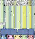
![[Uncaptioned image]](/html/2008.13556/assets/x1.png) An illustration of a smartwatch after querying all
restaurants in the near surrounding of a user. The three rows of displays show the labeling methods that we present in this paper; multi-page boundary labeling topmost, sliding boundary labeling centrally and stacking boundary labeling bottommost.Map tiles by Stamen Design, under CC BY 3.0. Data by OpenStreetMap, under ODbL.
\vgtcinsertpkg
Introduction
In the last years devices such as smartphones and smartwatches have
conquered our daily life and have made digital maps available at any
time. However, due to the small screen sizes, the presentation of
spatial information on such devices demands the development of new and
innovative visualization
techniques.
As an example, take a digital map that shows the results of a query for
restaurants in the near surroundings of the user;
see Zoomless Maps: External Labeling Methods for the Interactive Exploration of Dense Point Sets at a Fixed Map Scale. Desktop systems and tablets typically offer
enough space to place labels for an appropriately large selection of
restaurants still preserving the legibility of the background map. In
contrast, for small-screen devices—especially for
smartwatches—this is hardly possible as the screen may take
only few labels without covering the map too much.
An illustration of a smartwatch after querying all
restaurants in the near surrounding of a user. The three rows of displays show the labeling methods that we present in this paper; multi-page boundary labeling topmost, sliding boundary labeling centrally and stacking boundary labeling bottommost.Map tiles by Stamen Design, under CC BY 3.0. Data by OpenStreetMap, under ODbL.
\vgtcinsertpkg
Introduction
In the last years devices such as smartphones and smartwatches have
conquered our daily life and have made digital maps available at any
time. However, due to the small screen sizes, the presentation of
spatial information on such devices demands the development of new and
innovative visualization
techniques.
As an example, take a digital map that shows the results of a query for
restaurants in the near surroundings of the user;
see Zoomless Maps: External Labeling Methods for the Interactive Exploration of Dense Point Sets at a Fixed Map Scale. Desktop systems and tablets typically offer
enough space to place labels for an appropriately large selection of
restaurants still preserving the legibility of the background map. In
contrast, for small-screen devices—especially for
smartwatches—this is hardly possible as the screen may take
only few labels without covering the map too much.
The challenges posed by limited space for label placement are often softened by interactive map operations such as panning and zooming. They provide the user with the possibility of exploring the map by digging into its details. Hence, when there is too much information on the screen or the user is interested in some details, he or she can enlarge the map creating more space for the user’s area of interest. In particular, with such interactive operations no information is lost, as any label can be displayed by zooming in far enough. However, this might easily become cumbersome. Furthermore, the loss of the map’s context is an additional major drawback, which is particularly severe on small-screen devices. While the user enlarges the area of interest, information about the surroundings gets lost. In the example of searching for restaurants the user might need to zoom in and out repeatedly to first find the preferred restaurant and then to locate it on the entire map.

In this paper, we investigate labeling methods for zoomless maps. Such maps reduce the necessity for zooming the map by providing the user with additional interaction techniques that can be used for browsing the content of a temporarily fixed section of the map [12]. They implement the visual information-seeking mantra by Shneiderman [31]: overview first, zoom and filter, then details-on-demand; see Figure 1. In terms of application, starting with an overview map, the user first zooms and pans the map obtaining an adequate map of the area of interest (e.g., the city center). In a second step, the user applies the additional interaction techniques to browse all information (e.g., all restaurants) contained in the overview map keeping the view of the map fixed. Hence, the user has an overview of the entire area of interest at any time without the need of zooming in for additional information.
The labeling methods that we present in this work implement such additional interaction techniques and allow the user to display all labels successively without excluding any information beforehand. In the running example of searching for restaurants not all labels are presented at the same time, but the user can consecutively view them while keeping the displayed map region fixed. Hence, the user can systematically explore a region and can be finally sure to have obtained all information.
From a visualization point of view, placing the labels internally on the map leads to occluded map content. Especially, when using pictograms or even small images as labels, internal placement can quickly reach its limits in terms of legibility. Moreover, internal labeling does not provide the possibility of presenting labels in a specific order, e.g., with respect to the ratings of the labels’ point features.
Hence, we follow the idea to place labels at the bottom of the map in order to avoid hiding map content. We visually associate the labels with their point
features111As we only consider points as features but no other
types (e.g., lines and areas), we call point features more shortly features in the
remainder. by connecting them via a thin curve, also called
leader. Placing the labels alongside the boundary of a
rectangular map or figure is known in the literature as boundary
labeling, which is a special case of external
labeling [5]. For small-screen devices the number
of labels that can be placed at the bottom of the map is typically
small – in our experiments we set . Hence, in contrast to
previous work on boundary labeling, which has mostly considered static
labelings [5], we create and optimize the labelings for
user interaction. We consider the following three
labeling methods that offer the possibility of interactively
exploring the information by browsing through the labels222A
demo of all three labeling methods can be tried out on
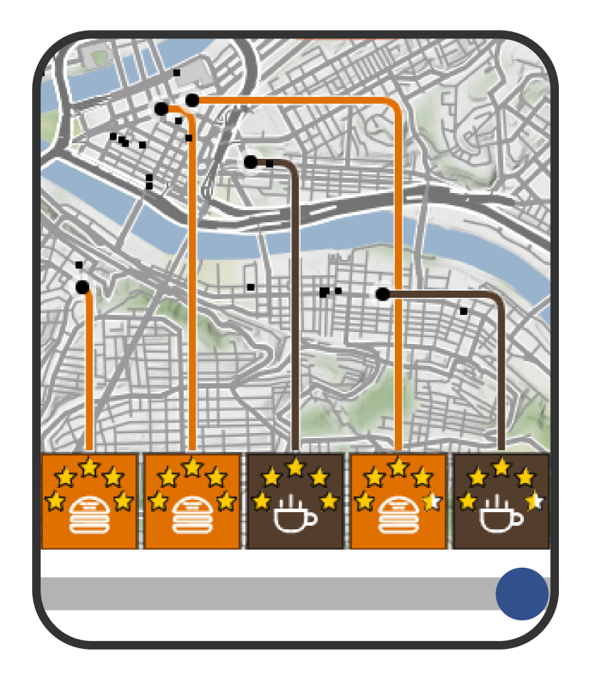
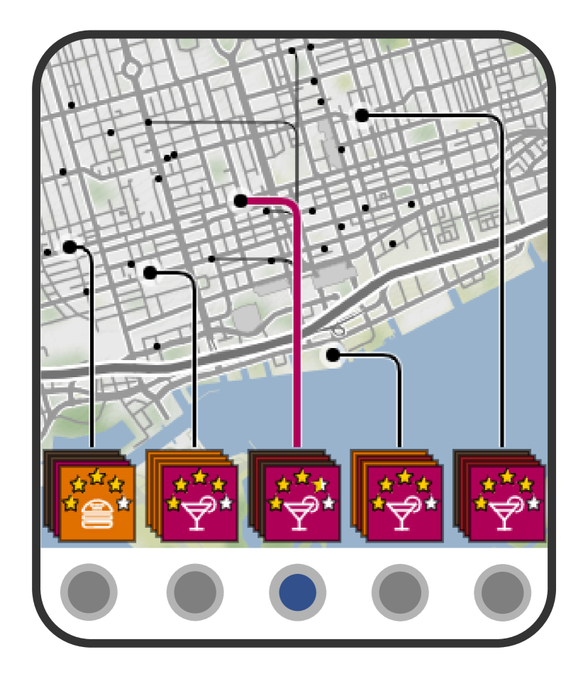
https://www.geoinfo.uni-bonn.de/interactive-boundary-labeling; for an illustration333The control bar shall illustrate the interaction by the user and can be omitted. see Figure 2. Each method offers advantages that can be beneficial in various use cases.
| Multi-Page | Sliding | Stacking | |
|
Las Vegas |

|

|
|
|
Pittsburgh |
|

|

|
| (a) | (b) | (c) |
-
L1
Multi-page boundary labeling. This labeling method distributes the labels over multiple pages such that each page consists of a boundary labeling; see Figure 2a. The user can navigate through the sequence of pages displaying at most labels in each step. Hence, after steps the user has obtained all pages and labels. Following Gedicke et al.[12], who considered a similar setting for placing labels internally, we call such a sequence of pages a paging of the labels. We present an algorithm for creating pagings optimizing both the order of the labels with respect to the importance of the features as well as the leader length. The distribution of labels on pages allows a user to gather information with a small number of interactions and to quickly locate individual labels.
-
L2
Sliding boundary labeling. This labeling method arranges the labels in a single row that can be continuously slid along the bottom of the map; see Figure 2b. Only the labels directly below the map are displayed to the user. However, this may easily lead to leaders that intersect or closely run in parallel. Using a graph-based model, we therefore optimize the order of the labels in this sequence taking into account the importance of the labels, the number of crossings as well as the vertical distance between two leaders. Since sliding boundary labeling supports continuous animation, users can easily trace changes in the labeling.
-
L3
Stacking boundary labeling. This labeling method creates stacks of labels below the map; see Figure 2c. We distribute the labels such that each label belongs to exactly one stack and the leader length is minimized. The topmost label of the stack is connected to its feature via a leader. When the user clicks on the stack the topmost label is pushed underneath the bottommost label. Hence, the second topmost label moves up and is then connected to its feature. Since each stack can be operated independently, stacking boundary labeling provides the possibility of creating customized labelings.
From a more technical point of view, we provide a generic framework, which subsumes all three labeling methods. This allows us to define mathematical optimization problems expressing these labeling methods in a unified way. For all three variants we present algorithms that yield optimal solutions. This provides us with the possibility of evaluating the underlying labeling methods independently from the applied algorithms. In contrast to previous work on boundary labeling, which mostly assumes specialized settings (e.g., only -shaped leaders are allowed, or the algorithms work only for single optimization criteria such as total leader length), our framework allows us an easy adaptation to any boundary labeling style and the consideration of multi-criteria objectives. In our evaluation we point out that none of the labeling methods prevail the others, but have their pros and cons depending on the application. We analyze them in greater detail in order to give the reader a simple way to select an appropriate technique for the specific purposes. Further, as some of the algorithms are rather slow and are developed for evaluation purposes only, we also present simple heuristics that yield near-optimal results fast enough for interactive operations.
The paper is structured as follows. After discussing related work (Section 1), we present an expert study (Section 2) on the three labeling methods. We conducted the study at an early stage of the algorithmic development to fine-tune the methods and objectives of the optimization problems. Subsequently, we present a mathematical model (Section 3) that we use to implement our labeling methods (Section 4–6). Finally, we evaluate our algorithms on real-world data (Section 7).
1 Related Work
Mobile cartography is a challenging field of research, especially since the available space and the interaction capacities for visualizing spatial information are limited. For presenting spatial content on mobile devices, a broad range of criteria is considered. In the field of mobile applications, Reichenbacher et al. [29] take the geographical context into account and propose methods for assessing the geographical relevance of spatial objects. Integrating further context such as physical, temporal and user-dependent criteria, Pombinho et al. [27] introduce a framework for mobile visualization. Usually, the requirements for the visualization in mobile cartography relate to the tasks that a user wants to accomplish [28]. For many specific tasks such as pedestrian navigation [26, 35] and annotating map content [15, 36, 12] research has already focused on small-screen devices. Especially in exploration tasks visualizations tend to be visually cluttered. Korpi and Ahonen-Rainio [19] systematically review reduction methods based on cartographic operations such as selection, aggregation and typification.
Another possibility for clutter reduction is providing the user with interaction techniques. Zooming is one of the most established and important interactions in digital maps, as it is both an intuitive and powerful tool for exploring the content of the map. Thus, the automated creation of digital maps that provide zooming has been an important subject of research in computational cartography. New algorithms for map generalization and label placement have been developed that ensure certain criteria of consistency over a large range of scales and, thereby, help users to keep track of the changes that occur in a map during zooming [3, 4, 2, 8, 30, 32, 33, 13]. Further, algorithms for continuously morphing [23] as well as algorithms for gradually transforming [25] two maps of different scales into each other have been proposed. Still, zooming becomes cumbersome when it is the only means for exploring the details of the map. This particularly drops the last integral part, namely details-on-demand, of the visualization mantra overview first, zoom and filter, then details-on-demand by Shneiderman [31].
Different tools have been proposed for reducing the necessary amount of zooming. One of them makes use of a lens, e.g., implemented as a simple circle, which the user can move over the map. Only features that are contained in the lens are annotated with labels, which are placed outside of the lens and are connected by thin leaders with their features. However, often there is not enough space in the close surroundings of the lens to show all labels without overlaps. Fekete et al. [9], Balata et al. [1] and Heihnsohn et al. [17] therefore place the labels in the extended margins of the lens, which is suitable for desktop systems but not for small-screen devices. Other strategies that keep the labels close to the boundary of the lens either select a conflict-free subset of labels [10, 16] or allow the labels to overlap [22].
Gedicke et al.[12] take a different strategy and distribute the labels over multiple pages, placing them on the map close to their features. This, however, requires rather small labels to keep the background map legible. We follow the core idea of showing not all labels at the same time, but enhance this concept with boundary labeling and interaction.
From an algorithmic point of view, Bekos et al. [6] introduced the first formal model for boundary labeling, which assumes that the map is rectangular and the labels are placed alongside of the boundary of the map. This was the starting point for a plethora of follow-up works [5]. A vast majority of them present highly specialized algorithms that are targeted at static figures and maps without providing any user interaction. As an exception, Nöllenburg et al. [24] consider boundary labeling for dynamic maps taking zooming into account. In contrast to previous work, we present a framework that supports different styles of boundary labeling without the need to change the underlying algorithms. For a detailed survey on external labeling techniques we refer to [5].
2 Expert Study
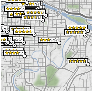
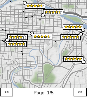
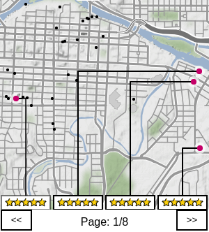
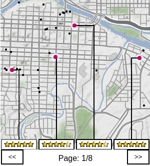
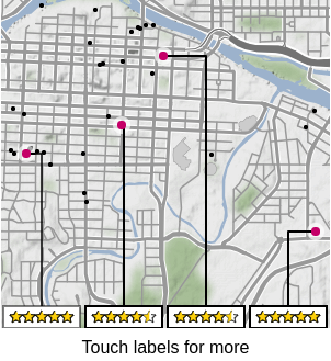
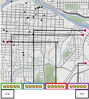
We conducted a preliminary study on the proposed visualization techniques. We aimed at improving our methods and verifying whether the design criteria from literature are valid for the proposed interactions. By discussing the methods with experts in an early stage, we identified inconsistencies before fine tuning the algorithms. The study involved nine experts in the fields of visualization, cartography and computational geometry. We presented the different visualizations in a web-browser, simulating a smartwatch444https://www.geoinfo.uni-bonn.de/interactive-boundary-labeling; see Figure 3. We asked the experts to use this simulation envisioning the following scenario: A user searches for restaurants in Calgary via his or her mobile device. The restaurants are labeled with their star rating. In order to maintain orientation within the city despite the small screen, all restaurants should be labeled without the user having to zoom in. We presented six different methods that address this problem. The first method, which we call Internal, simply places all labels with the bottom-right corner at their features in increasing order regarding their star rating. This method does not resolve conflicts. The second method, which we call InternalPaging, is an adaptation of the technique presented by Gedicke et al. [12]. This method distributes the labels on multiple pages and places them internally. We applied a four-position model for the placement of the labels, i.e., either the upper-left, upper-right, lower-left or lower-right corner of the label coincides with the feature. For the optimization we took into account both the distribution of the labels on the different pages and the position of the label. For optimizing the distribution we maximized the star rating on the first pages and further maximized the minimal number of labels on a page [12]. The third method, which we call BoundPaging1, and the fourth method, which we call BoundPaging2, use the algorithms for multi-page boundary labeling presented in this paper. BoundPaging1 purely optimizes the star rating on the first pages, while BoundPaging2 optimizes the balance between star rating and the total leader length. The fifth method, which we call BoundStacking, and the sixth method, which we call BoundSliding, present a stacking and sliding boundary labeling, respectively. Both were created manually. We emphasize that BoundSliding was intersection-free but there were gaps between consecutive labels to avoid leader crossings.
For the simulation we chose a screen size of 300px 300px, which is a common size for smartwatches [18]. The data set contains 32 restaurants. In contrast to the labels presented in Fig. Zoomless Maps: External Labeling Methods for the Interactive Exploration of Dense Point Sets at a Fixed Map Scale–2, the labels in the study only contained the restaurants’ star rating, but no additional symbol. All methods were implemented without continuous animations, so that BoundSliding could not develop its full potential concerning the traceability of changes. To support the user tracing individual labels during interaction, we colored the labels’ outlines differently.
We asked the experts to rate the following five statements from 1 (disagree) to 4 (fully agree).
-
S1
The method gives me quick access to the well rated restaurants.
-
S2
The visual association of labels and points is sufficiently clear.
-
S3
The map content needed for orientation, is not too much covered.
-
S4
The assignment of the restaurants to front or back pages sufficiently reflects the star rating.
-
S5
The shorter guide lines in BoundPaging2 lead to an improved visualization compared to BoundPaging1.
We computed the average for each statement; for S1–S3 see Table 1, for statement S4 we obtained 3.67 0.71 for BoundPaging1 and 2.72 0.67 for BoundPaging2, and for S5 we obtained .
| Experiment | S1 | S2 | S3 |
|---|---|---|---|
| Internal | 2.44 1.24 | 2.22 1.09 | 1.44 0.53 |
| InternalPaging | 3.56 0.88 | 3.56 0.73 | 3.11 0.78 |
| BoundPaging1 | 3.00 1.22 | 2.78 0.83 | 3.83 0.35 |
| BoundPaging2 | 2.11 0.60 | 3.11 0.78 | 3.94 0.17 |
| BoundStacking | 1.78 0.67 | 3.11 0.93 | 3.83 0.35 |
| BoundSliding | 2.56 1.24 | 2.78 0.97 | 3.83 0.35 |
Concerning statement S1 the experts liked InternalPaging and BoundPaging1 most, and BoundPaging2 and BoundStacking least. This result corresponds to the fact that for InternalPaging and BoundPaging1 the distribution on different pages is strictly in the order of the star ratings. For BoundPaging2 and BoundStacking this is not the case. Again, for S2 InternalPaging is best-rated and least favored is Internal which allows overlapping labels. For S3 methods using external labeling performed best, which is most likely explained by the fact that the labels are placed outside of the map and the leaders merely cover the map. The statements S4 and S5 only concern BoundPaging1 and BoundPaging2. In the experts’ opinion BoundPaging1 fulfills S4 substantially better than BoundPaging2. But for BoundPaging2 there is still a tendency that S4 is sufficiently fulfilled. With varying opinions S5 was rated with on average.
Besides rating the statements, we asked the experts to further comment on the methods. Commonly mentioned was that the number of labels was rather small and that BoundStacking was not intuitive.
The study showed that the interactive methods using boundary labeling were accepted well by the experts. In comparison to InternalPaging, the boundary labeling in general performed better for S3, while InternalPaging performed better for S1 and S2. Overall, we emphasize that the aim of this study was not to compare InternalPaging against BoundPaging1, BoundPaging2, BoundStacking and BoundSliding. Both internal and external boundary labeling have advantages and disadvantages, but non out-performs the other.
As a conclusion we came up with several improvements for our labeling methods: (1) we visualize the labels as actual stacks in BoundStacking; (2) we enrich the information displayed in a label by additionally visualizing the restaurants’ category (the star rating can be visualized more compact); (3) we use squared labels; (4) we strongly focus on a strict order of the star rating; see Zoomless Maps: External Labeling Methods for the Interactive Exploration of Dense Point Sets at a Fixed Map Scale and Figure 2. Besides these general adaptations we have mainly made adaptations to BoundSliding: (1) we use a continuous sliding animation, aiming to improve S2; (2) we forbid gaps and consider intersections as a soft, rather than a hard constraint which aims to improve S1 knowing that it might impair S2; (3) we maximize the vertical distances of neighbored features which aims at improving S2. Considering these improvements we obtain the labeling methods L1, L2, and L3.
3 Algorithmic Framework
#
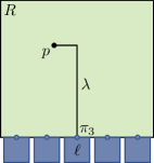


In this section we introduce an algorithmic framework that serves as a basis for our three labeling methods L1 – L3; see Section 1. We assume that we are given a set of features within a pre-defined rectangular region that we refer to as map in the following; see 4a. We introduce a weight function that assigns a weight to each feature . Further, each feature in the map is allocated to a rectangular label that describes the feature. We assume that all labels are uniformly sized. As the available space on a small-screen device is limited, we place labels at the bottom side of the map for features. More precisely, we define fixed positions at the bottom side of the map, which we call ports. We denote the set of ports by and assume that they are ordered from left to right. We attach a label to a port by placing the label such that the midpoint of its upper side coincides with . The ports are arranged such that the attached labels do not overlap. Moreover, we visually associate a feature and the port of an attached label by connecting with by a leader. Although the framework covers any kind of leader, we use so-called po-leaders [5] in our experiments. Such leaders consist of two line segments. The first starts at the feature and is parallel (p) to the bottom side of the map. The second ends at the port and is orthogonal (o) to the bottom side of the map.
We model the assignment between features and ports by a state that maps each port on a feature. We denote the set of all states by . Further, a state contains a feature if a port exists with . A state is crossing-free if the leaders that connect the ports with the contained features of do not intersect each other.
In the proposed labeling methods we describe a labeling as a sequence of states. We require that each feature is contained in at least one state of . Further, we call a labeling crossing-free if all its states are crossing-free. Based on the knowledge gained from the expert study, we consider four criteria for labelings.
-
C1
Important features should be contained in the first states.
-
C2
Crossings of leaders should be avoided.
-
C3
Vertical distances between the horizontal segments of different leaders in the same state should be large.
-
C4
Leaders should be short.
Depending on the labeling method, we strictly enforce these criteria or express them as cost functions rating each state with separately. We discuss the cost functions in the following.
Criterion C1 is described as weight cost with
Important features preferably occur in a state with a small index , while less important features are assigned to states with higher indices.
Criterion C2 is described as crossing cost with
The term denotes the number of crossings between leaders in state . We normalize the number of crossings by the maximum number of possible crossings per state.
Criterion C3 is described as distance cost with
The set contains all pairs of features whose leaders in have horizontal segments partially running above each other. Hence, states with horizontal leader segments running close above each other have higher distance costs than states with well separated leaders. We average the cost by the maximal size of .
Criterion C4 is described as leader cost with
The term denotes the length of the leader that connects the port with the feature . We normalize the length of the leaders by the screen width and height. The relevance of a state decreases exponentially with increasing index , so that short leader lengths are given more priority on front states than on back states.
For each of the three labeling methods we use , , and to compose a bicriteria cost function that balances two of those cost functions by means of a factor . We call the cost of a labeling . We restricted ourselves to bicriteria cost functions to be capable of controlling the effects of the optimization on the resulting labeling. More precisely, we use the two criteria that affect each method most as soft constraints and express the others as hard constraints if this is reasonable. We argue for the actual choice in the following sections.
4 Multi-page boundary labeling
In multi-page boundary labeling the labels are distributed on multiple pages such that each page labels a distinct set of features (see 4b). Each page corresponds to a state in a labeling with ; in the case that , we introduce dummy features that do not influence the overall solution. We say is a multi-page boundary labeling if each feature is contained in exactly one state and it is crossing-free (C2). Among all multi-page boundary labelings, we search for one that optimizes the weight cost (C1) and the leader cost (C4). We do not consider the vertical distances between features (C3), as we deem such distances mostly problematic in combination with crossings. Based on and , we define the cost of a multi-page boundary labeling as
where balances the leader and weight cost of . For and , only the feature cost and the leader cost are considered, respectively. For a single state of we further define . Due to the linearity, we have .
We show that the problem of finding a multi-page boundary labeling can be transformed into finding a perfect matching in a bipartite graph. At first, we observe that for a set of features and ports the problem reduces to computing a one-sided boundary labeling with minimum total leader length for a single page. Such a labeling can be computed in time [7] – no matter whether the length of the leader is normalized or not. We reformulate this as follows.
Observation 1
Let be features and label ports. Let be a not necessarily crossing-free state with minimal costs over all states of and . There exists a crossing-free state with .
Observation 1 holds because the number of features corresponds to the number of ports. Hence, only the leader cost is considered, but not the weight cost. Using Observation 1, we divide the computation into two steps; first we find a cost-minimal possibly non crossing-free solution, and in the second step we resolve the crossings on each page.
The first step corresponds to finding a perfect matching in a bipartite graph. In general, let be a weighted bipartite graph, i.e., is partitioned into two disjoint sets and and each edge connects a vertex with a vertex . A perfect matching in is a subset of such that each vertex is incident to exactly one edge of the subset. A minimum-weight perfect matching is a perfect matching that minimizes the sum of the weights over all selected edges.
For multi-page boundary labeling the vertex set consists of the vertices where is a feature and the set consists of the vertices where is a pair of a port and a state ; see Figure 5. Further, is a complete bipartite graph. For each edge that connects the vertices and , we set the weight equal to
To solve the multi-page boundary labeling allowing crossings, we compute a perfect minimum-weight matching in , which can be done in time [20, 21]. In our implementation, we used a linear programming approach, which is also a common method [14].
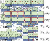
In the second step, we apply the algorithmic approach presented by Benkert et al. (2009)[7] for each state to find a crossing-free labeling with minimal leader length. We also use this approach for the stacking boundary labeling and discuss it in Section 6 in greater detail.
5 Sliding boundary labeling
In sliding boundary labeling the labels can be moved along the bottom side of the map. From a technical point of view, we assume that the labeling is given as a sequence of states; see 4c. The interaction of sliding the labels then corresponds to an animated transition between consecutive states. To guarantee a continuous flow of labels, we require that from one state to the next state the labels are shifted to the left by one port and a new label appears at the rightmost port. More formally, we say that the transition from to is valid, if for all and .
Since—except for the last labels—each label is shifted once from the rightmost to the leftmost port, we do not consider the leader length (C4). Instead, we aim for a labeling that minimizes both the crossing cost (C2) and the distance cost (C3). For we define the cost of a labeling as
In the following, we present an exact approach that yields the optimal solution as well as a fast and simple heuristic.
5.1 Exact Approach
For obtaining an optimal sliding boundary labeling we use a graph-based method by modeling our optimization problem as an constrained orienteering problem [34]. Given a graph in which each vertex has a score and each edge a length, a source and a target vertex, the orienteering problem asks for a path from the source to the target such that the total score along the path is maximized and a given length is not exceeded. With some adaptations on the original problem definition this path represents a labeling. We define an integer linear programming (ILP) formulation that expresses the problem of finding an optimal labeling as a linear objective function subject to a set of linear constraints. In general, solving such formulations is NP-hard [11]. However, there exist solvers that handle many of such formulations in adequate time. We present a formulation that models the problem as a flow network. The idea is to send a unit from a source to a target vertex via the graph.
We present now the details of our approach. Let be a directed graph containing a vertex for each state . Further, contains a source vertex and a target vertex . Each state is connected with the source by an edge and with the target by an edge . Moreover, a pair of states is connected by a directed edge if and only if the transition from state to state is valid. We aim for a path from to representing a labeling; see Figure 6.
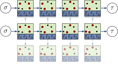
Next, we describe our ILP formulation. For each directed edge we introduce a binary variable . We interpret such that if and only if the transition of state to state is used in the labeling. Additionally, we introduce a variable for each state with being the number of states. We use to ensure that the sub-graph defined by the edges with is actually one connected component forming a path from to . We denote the set of all states that contain a feature by . Further, we define to be the set that contains any edge whose source does not contain , but whose target contains , i.e., . In order to model a path in that represents a labeling we introduce the following constraints. (1) (2) (3) (4)
| (5) | ||||
| (6) |
Constraint 1 and Constraint 3 ensure that the path begins at the source and ends at the target by enforcing that exactly one transition from and one transition to is used. Hence, in terms of the flow network, exactly one unit leaves the source and one unit reaches the target. Constraint 2 ensures that each state can be the origin of at most one transition, i.e., at most one unit leaves each state. To preserve the flow, Constraint 4 implies that if a unit reaches one state, it also leaves this state. As we aim for one connected path through , we introduce Constraint 5, which guarantees that the states are numbered in ascending order along the path. Hence, no cycles can be created. To ensure that the path corresponds to a labeling, Constraint 6 guarantees that each feature is labeled at least in one state and that it only appears in consecutive states. Subject to Constraint 1–6 we minimize
| (7) |
Let be the path from to . Going along we obtain a sequence of states which forms a sliding labeling such that is minimal.
5.2 Heuristic Approach
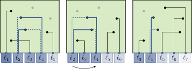
We present a simple and fast heuristic for sliding boundary labeling that is based on the local search strategy hill climbing. Starting from an initial solution, such methods iteratively perform local changes in the current solution to obtain neighboring solutions. Such a neighboring solution is accepted as the new current solution if it improves the objective. The algorithm terminates if a pre-defined number of iterations is reached or no more neighboring solutions of higher quality exist.
For the initial solution we apply a simple first-fit strategy: we create an arbitrary order of the features and define a state as for . Hence, sliding the labels from right to left, the features are labeled in that order. We iteratively improve that labeling by performing local changes. We obtain a neighboring solution by swapping the assignments and of two randomly chosen features and , i.e., after this swap we have and . For an illustration of a swap see Figure 7. If such a swap improves the value of the objective function, it is applied obtaining a new solution. The algorithm continues with performing such swaps until a pre-defined number of iterations is reached or no more neighboring solutions of higher quality exist.
6 Stacking boundary labeling
The stacking boundary labeling is characterized by its interaction technique. Instead of having one pre-defined sequence of states, the features are partitioned into groups; each assigned to one stack. Hence, we have an own sequence of states for each single stack, where each state consists of a single feature. By clicking on one label, its port is connected to the next feature in the stack.
We call with the stack of port . A feature is contained in a stack at position if . A stacking boundary labeling consists of the set of stacks . We require that the features are evenly distributed over all stacks555We assume . If this is not the case we insert dummy feature points., i.e., , that each feature is contained in exactly one stack at one position, and that the labeling is crossing-free (C2). Among all stacking boundary labelings we search for the one that optimizes the weights of the features on the first stack positions (C1) and the length of the leaders (C4). As there exists a state for every two features of different stacks in which they are labeled simultaneously, we do not consider the vertical distance (C3). The user can improve the visualization by clicking on the labels of features that are vertically close together.
As the primary objective for partitioning the features into groups, we optimize the leader length globally for as follows.
As the secondary objective for each sequence, we optimize Criterion C1 by ordering the features of each stack by their weight. We show that the problem can be transformed into a static boundary labeling problem. We introduce each port of our stacking boundary labeling problem times; see 8a. Further, we adapt the definition of a crossing; we say that two leaders that start at the same port cannot cross. A solution of the first step of the stacking boundary labeling problem is a crossing-free assignment with minimal leader length between the labels’ ports and features. The approach by Benkert et al. [7] solves this problem in time. In the approach the map is partitioned into strips induced by vertical lines through each label’s port and feature; see 8b. The strips are categorized into leftwards and rightwards directed strips by a comparison of the number of labels and the number of features to the right and left. Each consecutive set of leftwards directed strips is solved with a sweep line approach from right to left. Each time the sweep line passes a feature, it is inserted into a list which is ordered by the features’ -coordinates. Every time the sweep line intersects a port, this port is assigned to the lowest feature contained in . The rightwards directed strips are solved with a symmetric approach. Finally, we sort each stack by the weight of the features.
A stacking labeling corresponds to a multi-page labeling by assigning the -th label of each stack to the -th page, i.e., .

7 Evaluation
Following, we present experiments evaluating our labeling methods on real-world data focusing on quantitative criteria and performance.
We simulated the use case of querying restaurants with a smartwatch visualizing the result on a map. At first, we evaluate each labeling method individually. In particular, we identify a suitable choice of describing the sweet spot between the contradictory optimization criteria. Further, we show that it pays off to optimize the criteria C1–C4 by comparing the algorithms’ results with the worst and best cases considering each criterion. For a cost function and two labelings and we define their relative cost as
We use the relative cost to compare a labeling with another labeling that is optimal with respect to one or multiple of the criteria C1–C4. Finally, we compare the labeling methods with each other emphasizing their strengths and weaknesses.
We use the following experimental setup. For the smartwatch we assume a screen size of 300px 300px, which is a common resolution [18]. The displayed map comprises roughly 5733m 5733m. This extent is a good compromise between a broad overview of the area of interest and the possibility of identifying the location of the restaurant.
We obtained the data of the restaurants from Yelp666www.yelp.com for the cities Calgary (CA), Las Vegas (US), Montreal (CA), Pittsburgh (US) and Toronto (CA). Each restaurant is given with its location and star rating. The rating varies between one and five; half-stars are also allowed. We normalize the ratings obtaining weights in the interval . We create 100 instances of different map sections each having 30 randomly sampled features; see Figure 2 for examples. We use five labels (), each with a size of 60px60px. To make the visualization more realistic we extend the data with categories; e.g., pizza restaurant. We note that this has no impact on the algorithms nor the evaluation.
The implementations were done in Java, and the ILP and LP formulations were solved by Gurobi777www.gurobi.com 8.1.0. We ran the experiments on a Intel(R) Xeon(R) W-2125 CPU clocked at 4.00GHz with 128 GiB RAM. Considering a server-client communication as the use case for our algorithms, we performed the computations on a server system.
7.1 Multi-page Boundary Labeling
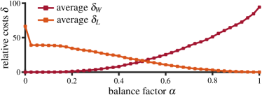
For the multi-page boundary labeling, we evaluate the weight cost (C1), the leader cost (C4), and the distance cost (C3) for different values of . The weight cost and leader cost are considered in the objective where balances those. For the experiments, we sampled in the range with a step width of . We denote the set of the resulting values by and a multi-page boundary labeling for by .
Optimized Criteria C1 and C4
We consider the relative weight cost of a labeling and the labeling with minimal weight cost; see Figure 9. Similarly, we define the relative leader cost for a labeling and the labeling being the solution with minimal leader cost . We obtain that the difference between the relative leader cost for and is remarkably large. When comparing this to the average it is noticeable that is still optimal for . Hence, by choosing instead of , the cost for is still minimal, while is also considered. Thus, when ordering the features by their weights is strictly required—as derived from the expert study—we recommend to choose . Moreover, the relative costs of both criteria intersect at . Hence, we deem to be a suitable compromise between optimizing the weight cost and leader cost.
Non-optimized Criterion C3
For the multi-page boundary labeling, we do not consider the distance cost in the objective. We analyze all pairs of leaders which are labeled on the same page and for which the horizontal parts of the leaders run above each other. At first, we evaluate the size of in relation to the overall number of leader pairs on the same page. On average of the leader pairs on the same page horizontally run above each other. In particular, the ratio is similar for all values of . Moreover, we analyze the ratio of leader pairs in with a vertical distance smaller than pixels with respect to the size of . This ratio varies between for , and for . This means, that at most of the of leader pairs which have horizontal segments lying above each other, have a vertical distance under px. Since the multi-page boundary labeling provides static pages, this result seems to be appropriate to distinguish the leaders.
7.2 Sliding Boundary Labeling
Our study (see Section 2) showed that experts generally recommend to strictly label the features in descending weight order. Hence, we consider a special case of sliding boundary labeling in which we enforce Criterion C1 as hard constraint. While the overall weight order is preserved, we optimize the order within groups of features having the same weight regarding the cost function . We modify our exact approach such that the graph only contains states satisfying Criterion C1. Hence, is the set of states in which the features are assigned to the ports from left to right in descending weight order.
We also adapted the heuristic as follows. When constructing an initial solution, we sort the given features in descending weight order. Further, when obtaining neighboring solutions, we only swap the assignments and of two randomly chosen features and if . We use iterations as termination criterion, which has proven to be a suitable choice in preliminary experiments. For each instance and each considered weighting we run our heuristic five times and build the arithmetic mean of the results.
Evaluation of Exact Approach
We first evaluate our exact approach with respect to both optimized criteria, i.e., the crossing cost (C2) and the distance cost (C3). We run the approach for . For and we only optimize C3 and C2, respectively. Further, we use as an intermediate value balancing both criteria. When running our exact approach with a number of labels per state, the storage capacity of the used system is exceeded. By reducing the number of labels to , we are able to successively run the approach on all 100 instances. We argue that limiting the number of labels to four still models a realistic setting, in which a high number of leader crossings and small vertical distances may occur in the worst case.
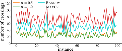
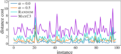
We investigate the potential of optimization with respect to both considered criteria. To that end, we additionally determine the maximum possible costs and of both criteria. More specifically, instead of minimizing the objective function in our ILP formulation, we maximize it for and , respectively. We denote the results by MaxC2 for and by MaxC3 for . Further, we created for each instance a labeling in which features of the same weight group are ordered randomly; we refer to them as Random. The results are found in Figure 10 and Figure 11. The crossing costs are displayed without normalization so that they show the absolute number of crossings.
We observe that the non-normalized leader cost lies between () and (MaxC2) on average. Hence, by choosing the number of leader crossings can be reduced by in maximum. When considering the trade-off , the number of leader crossings can still be reduced by on average. Compared to a randomly generated labeling (Random), the number of leader crossings is reduced by on average.
Concerning the distance cost of the optimal results for , MaxC3 and Random, we make a similar observation; see Figure 11. The average distance cost is in maximum and in minimum, which means that the distance cost can be reduced by in maximum. For the distance cost is still reduced by on average. Compared to a randomly generated labeling, with the distance cost is reduced by on average. These results show that both considered criteria C2 and C3 can be substantially optimized by an appropriate choice of .
Exact Approach vs. Heuristic
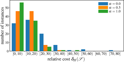
We evaluate the quality of our heuristic by comparing its results with the optimal results obtained from the exact approach. For each instance and each we compute the relative cost where is a labeling produced by the heuristic and is the optimal labeling for the same instance; see Figure 12. For and for of the instances the relative cost is less than . Further, and of the instances have relative costs less than for and , respectively. On average, the relative costs of the heuristic solutions are , and for , , and , respectively. In particular, for about of the quality of the optimal solution was reached on average. Hence, apart from some instances, our heuristic provides results that are sufficiently close to optimal.
Heuristic
Finally, we systematically analyze how the heuristic behaves for each (see Section 7.1). We denote the corresponding labeling by . As we do not take the exact approach into account, we use five labels for each state as also done in the other labeling methods.
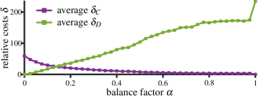
For evaluating Criterion C2 we consider for each labeling the relative crossing cost , where only takes Criterion C2 into account; see Figure 13. As we create by means of an heuristic, the relative cost can be negative. Similarly, we evaluate the relative distance cost , where only takes Criterion C3 into account. We obtain that the average relative crossing and distance costs are almost equal for . We deem this value of to be a suitable compromise between Criteria C2 and C3.
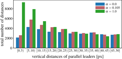
To further evaluate the extent to which Criterion C3 is optimized, we consider the distribution of vertical leader distances within a range of pixels for ; see Figure 14. We obtain that compared to the results in which only Criterion C2 is optimized () we can reduce the number of vertical leader distances smaller than five pixels by when optimizing C3 (). However, with we can still reduce these smallest leader distances by .
7.3 Stacking Boundary Labeling
We analyze both the weight costs (C1)—similar as done for the multi-page boundary labeling—and the distance cost (C3). Recall that a stacking boundary labeling can be interpreted as a multi-page boundary labeling. Hence, we can evaluate the relative weight costs where is a stacking boundary labeling and is the multi-page boundary labeling with minimal weight cost. On average the relative weight cost is with a standard deviation of . Hence, top rated features are nearly as equally distributed on the stacks as for the optimal multi-page boundary labeling. Put differently, we obtain a small number of interactions for exploring them. Moreover, we evaluate the vertical distances of the leaders that run horizontally above each other. Let be the set of all pairs of leaders with horizontal segments lying above each other and for which the leaders start at different ports. The ratio between the size of and the overall number of leader pairs starting at different ports is on average with a standard deviation of . The number of leader pairs in with a vertical distance smaller than five pixels is . Hence, on average we obtain a smaller number of leader pairs with horizontal segments running above each other and a smaller number of leader pairs with vertical distances under five pixels than for the multi-page boundary labeling.
| Key Property | Multi-Page | Sliding | Stacking |
|---|---|---|---|
| C1: weight | soft | hard | soft |
| C2: crossing | hard | soft | hard |
| C3: distance | – | soft | – |
| C4: leader | soft | – | soft |
| animation | discrete | continuous | discrete |
| change | labels | 1 label | 1 label |
7.4 Comparison
We finally compare the labeling methods providing decision support for deploying them in practice; see Table 2. In all methods one criterion is a hard constraint and two are additionally optimized. Hence, the enforced criterion can be interpreted as the primary design rule. For example, for crossing-free labelings multi-page and stacking boundary labeling are preferable. Further, the methods differ in their interaction techniques. Both multi-page and stacking boundary labeling are designed for discrete interaction, so that switching between two states involves no transitional animation. In contrast, sliding boundary labeling provides continuous animation, which supports the user in tracing changes. Another difference is the amount of change between each interaction step. For multi-page boundary labeling all labels are exchanged by completely different labels in each interaction step. In contrast, for the two other labeling methods only one label is exchanged. Hence, for multi-page boundary labeling less interaction is necessary to explore all information. On the other hand, by means of the two other labeling methods the user can adjust the labeling in small steps. In sliding boundary labelings the interaction is still strongly bounded, i.e., the labels are slid along in a specific order. Stacking boundary labeling provides less restricted interaction. The user can easily customize the displayed labeling by changing the topmost labels on the stacks.
| Setup | Multi-Page | Sliding | Stacking | |
|---|---|---|---|---|
| 10.58 2.89 | 44.30 0.52 | 10.51 3.51 | ||
| 83.53 11.18 | 53.53 0.60 | 71.10 4.92 | ||
| 7.67 3.09 | 75.47 0.93 | 8.72 3.93 | ||
| 85.58 12.53 | 96.20 1.82 | 74.06 5.40 | ||
For all methods we measured the running time of the heuristics for ports and point features; see Table 3. For multi-page boundary labeling and sliding boundary labeling, we averaged over all choices of . To further assess the impact of the number of ports and features on the running time, we also considered and . We observe that for each setting the running time is less than a tenth of a second, which we consider reasonable in terms of actual applicability. Altogether, no labeling method prevails over the others. The concrete application decides which of them is the preferable choice.
8 Conclusion
In this paper, we investigated three labeling methods that reduce the necessity of zooming by providing the user with the possibility of browsing through the labels without changing the displayed map in the background. For all three methods we presented algorithms that run fast enough for real-world applications on devices such as smartwatches. They enforce and optimize the Criteria C1–C4, which we have identified in an expert study. With a systematic and quantitative evaluation of the mathematical models and algorithms we laid the foundation for zoomless maps using external labeling. Altogether, this paper provides the following novel and scientific contributions.
-
•
New external labeling methods that allow a user to navigate through dense sets of points of interest in zoomless maps.
-
•
Design decisions for external labeling based on expert advice.
-
•
Generalization of the three labeling methods into a unified algorithmic framework.
-
•
Exact algorithms and fast heuristics for the optimization problems.
So far we have considered all three labeling methods under the assumption that the map is fixed. It is future work to investigate how the labeling methods can be combined with operations such as zooming and panning such that different frames have similar labelings. In terms of actual applicability, future work should additionally focus on how well the methods can be translated to interaction on an actual small-screen device. We finally emphasize that the presented methods are only a starting point towards more sophisticated labeling concepts.
Acknowledgements.
Partially funded by the Deutsche Forschungsgemeinschaft (DFG, German Research Foundation) under Germany’s Excellence Strategy – EXC 2070 – 390732324. Partially funded by Zoomless Maps: Models and Algorithms for the Exploration of Dense Maps with a fixed Scale of the German Research Foundation (DFG) [grant number 5451/6-1]References
- [1] J. Balata, L. Čmolík, and Z. Mikovec. On the selection of 2d objects using external labeling. In Human Factors in Computing Systems (CHI’14), pages 2255–2258. ACM, 2014.
- [2] L. Barth, B. Niedermann, M. Nöllenburg, and D. Strash. Temporal map labeling: a new unified framework with experiments. In Adv. in Geographic Information Systems (ACM-GIS’16), pages 1–10. ACM Press, 2016.
- [3] K. Been, E. Daiches, and C. Yap. Dynamic map labeling. IEEE Transactions on Visualization and Computer Graphics, 12(5):773–780, 2006.
- [4] K. Been, M. Nöllenburg, S.-H. Poon, and A. Wolff. Optimizing active ranges for consistent dynamic map labeling. Computational Geometry: Theory and Applications, 43(3):312–328, 2010.
- [5] M. Bekos, B. Niedermann, and M. Nöllenburg. External labeling techniques: A taxonomy and survey. Computer Graphics Forum, 38(3):833–860, 2019.
- [6] M. A. Bekos, M. Kaufmann, A. Symvonis, and A. Wolff. Boundary labeling: Models and efficient algorithms for rectangular maps. In Graph Drawing (GD’04), volume 3383 of LNCS, pages 49–59. Springer, 2004.
- [7] M. Benkert, H. J. Haverkort, M. Kroll, and M. Nöllenburg. Algorithms for multi-criteria boundary labeling. Journal of Graph Algorithms and Applications, 13(3):289–317, 2009.
- [8] M. Chimani, T. C. van Dijk, and J.-H. Haunert. How to eat a graph: Computing selection sequences for the continuous generalization of road networks. In Adv. in Geographic Information Systems (ACM-GIS’14), pages 243–252. ACM Press, 2014.
- [9] J.-D. Fekete and C. Plaisant. Excentric labeling: Dynamic neighborhood labeling for data visualization. In Human Factors in Computing Systems (CHI’99), pages 512–519. ACM Press, 1999.
- [10] M. Fink, J. Haunert, A. Schulz, J. Spoerhase, and A. Wolff. Algorithms for labeling focus regions. IEEE Transactions on Visualization and Computer Graphics, 18(12):2583–2592, 2012.
- [11] M. R. Garey and D. S. Johnson. Computers and Intractability: A Guide to the Theory of NP-Completeness. W. H. Freeman & Co., 1979.
- [12] S. Gedicke, B. Niedermann, and J.-H. Haunert. Multi-page labeling of small-screen maps with a graph-coloring approach. In Location Based Services (LBS’19), 2019.
- [13] A. Gemsa, B. Niedermann, and M. Nöllenburg. A unified model and algorithms for temporal map labeling. Algorithmica, 4 2020.
- [14] M. Grötschel and O. Holland. Solving matching problems with linear programming. Mathematical Programming, 33(3):243–259, 1985.
- [15] L. Harrie, H. Stigmar, T. Koivula, and L. Lehto. An algorithm for icon labelling on a real-time map. In Developments in Spatial Data Handling, pages 493–507. Springer, 2005.
- [16] J.-H. Haunert and T. Hermes. Labeling circular focus regions based on a tractable case of maximum weight independent set of rectangles. In Proc. 2nd ACM SIGSPATIAL International Workshop on Interacting with Maps (MapInteract’14), pages 15–21, 2014.
- [17] N. Heinsohn, A. Gerasch, and M. Kaufmann. Boundary labeling methods for dynamic focus regions. In IEEE Pacific Visualization Symposium (PacificVis’14), pages 243–247, 2014.
- [18] W. Jackson and Pao. SmartWatch Design Fundamentals. Springer, 2019.
- [19] J. Korpi and P. Ahonen-Rainio. Clutter reduction methods for point symbols in map mashups. The Cartographic Journal, 50(3):257–265, 2013.
- [20] H. W. Kuhn. The hungarian method for the assignment problem. Naval research logistics quarterly, 2(1-2):83–97, 1955.
- [21] J. Munkres. Algorithms for the assignment and transportation problems. Journal of the society for industrial and applied mathematics, 5(1):32–38, 1957.
- [22] B. Niedermann and J. Haunert. Focus+context map labeling with optimized clutter reduction. International Journal of Cartography, 5(2–3):158–177, 2019. Special issue of 29th International Cartographic Conference (ICC’19).
- [23] M. Nöllenburg, D. Merrick, A. Wolff, and M. Benkert. Morphing polylines: A step towards continuous generalization. Computers, Environment and Urban Systems, 32(4):248–260, 2008.
- [24] M. Nöllenburg, V. Polishchuk, and M. Sysikaski. Dynamic one-sided boundary labeling. In Adv. in Geographic Information Systems (ACM-GIS’10), pages 310–319. ACM Press, 2010.
- [25] D. Peng, A. Wolff, and J.-H. Haunert. Using the A* algorithm to find optimal sequences for area aggregation. In Adv. in Cartography and GIScience – Selections from the International Cartographic Conference 2017, pages 389–404. Springer, 2017.
- [26] M. Perebner, H. Huang, and G. Gartner. Applying user-centred design for smartwatch-based pedestrian navigation system. Journal of Location Based Services, 13(3):213–237, 2019.
- [27] P. Pombinho, M. B. Carmo, and A. P. Afonso. Adaptive mobile visualization-the chameleon framework. Computer Science and Information Systems, 12(2):445–464, 2015.
- [28] T. Reichenbacher. Adaptive concepts for a mobile cartography. Journal of Geographical Sciences, 11(1):43–53, 2001.
- [29] T. Reichenbacher, S. De Sabbata, R. S. Purves, and S. I. Fabrikant. Assessing geographic relevance for mobile search: A computational model and its validation via crowdsourcing. Journal of the Association for Information Science and Technology, 67(11):2620–2634, 2016.
- [30] M. Sester and C. Brenner. Continuous generalization for visualization on small mobile devices. In Developments in Spatial Data Handling (SDH’04), pages 355–368, 2004.
- [31] B. Shneiderman. The eyes have it: a task by data type taxonomy for information visualizations. In Visual Languages (VL’96), pages 336–343. IEEE, 1996.
- [32] R. Suba, M. Meijers, and P. van Oosterom. Continuous road network generalization throughout all scales. ISPRS International Journal of Geo-Information, 5(8), 2016.
- [33] P. van Oosterom and M. Meijers. Vario-scale data structures supporting smooth zoom and progressive transfer of 2D and 3D data. International Journal of Geographical Information Science, 28(3):455–478, 2014.
- [34] P. Vansteenwegen, W. Souffriau, and D. Van Oudheusden. The orienteering problem: A survey. European Journal of Operational Research, 209(1):1–10, 2011.
- [35] D. Wenig, J. Schöning, B. Hecht, and R. Malaka. Stripemaps: Improving map-based pedestrian navigation for smartwatches. In Human-Computer Interaction with Mobile Devices and Services (MobileHCI’15), pages 52–62, 2015.
- [36] Q.-n. Zhang and L. Harrie. Real-time map labelling for mobile applications. Computers, environment and urban systems, 30(6):773–783, 2006.