Machine learning for metal additive manufacturing: Predicting temperature and melt pool fluid dynamics using physics-informed neural networks

Abstract

The recent explosion of machine learning (ML) and artificial intelligence (AI) shows great potential in the breakthrough of metal additive manufacturing (AM) process modeling, which is an indispensable step to derive the process-structure-property relationship. However, the success of conventional machine learning tools in data science is primarily attributed to the unprecedented large amount of labeled data-sets (big data), which can be either obtained by experiments or first-principle simulations. Unfortunately, these labeled data-sets are expensive to obtain in AM due to the high expense of the AM experiments and prohibitive computational cost of high-fidelity simulations, hindering the direct applications of big-data based ML tools to metal AM problems.

To fully exploit the power of machine learning for metal AM while alleviating the dependence on “big data”, we put forth a physics-informed neural network (PINN) framework that fuses both data and first physical principles, including conservation laws of momentum, mass, and energy, into the neural network to inform the learning processes. To the best knowledge of the authors, this is the first application of physics-informed deep learning to three dimensional AM processes modeling. Besides, we propose a hard-type approach for Dirichlet boundary conditions (BCs) based on a Heaviside function, which can not only exactly enforce the BCs but also accelerate the learning process. The PINN framework is applied to two representative metal manufacturing problems, including the 2018 NIST AM-Benchmark test series. We carefully assess the performance of the PINN model by comparing the predictions with available experimental data and high-fidelity simulation results, , using finite element based variational multi-scale formulation. The investigations show that the PINN, owed to the additional physical knowledge, can accurately predict the temperature and melt pool dynamics during metal AM processes with only a moderate amount of labeled data-sets. The foray of PINN to metal AM shows the great potential of physics-informed deep learning for broader applications to advanced manufacturing. All the data-sets and the PINN code will be made open-sourced in https://yan.cee.illinois.edu/ once the paper is published.

1 Introduction

It has been widely believed that metal additive manufacturing (AM) can revolutionize mechanical, aerospace, and biomedical industries owing to its superior capability to print metals with complex geometries directly from digital models without the design constraints of traditional manufacturing routes. The market of metal AM has been growing significantly for the past decade. However, compared with the total manufacturing market, the industrial adoption of metal AM has not reached its expected potential due to a lack of reliable process-structure-property relationships. For the past several years, predictive computational models, in conjunction with in-situ and ex-situ measurements and monitoring [1, 2, 3], have been playing an indispensable role in enhancing the understanding of the process-structure-property relationship in metal AM. Federal agencies have also conducted several benchmark experiments, such as NIST AM-bench [4] and AFRL AM modeling challenge series [5], to facilitate the development of metal AM modeling tools.

Among various computational models at different scales and fidelity, thermal-fluid process simulation is not only an essential tool to understand the metal AM physics but also acts as a spearhead to derive the process-structure-property relationship. The metal AM process is intrinsically a multi-scale and multi-physics problem, involving rapid, complex, and coupled mass/flow/heat exchanges between gas, liquid, and solid phases, with large density ratios and complicated interfacial phenomenon. Current numerical simulation tools often employ mathematical models that couple Navier-Stokes equations and a heat transfer equation to capture the evolution of temperature and melt pool dynamics during manufacturing processes. For decades, the manufacturing community has been adopting computational methods that directly solve these mathematical models or their weak forms, based on spatial discretization (e.g., finite difference, finite volume, finite element, and mesh-free methods) and time-stepping.

The predictive capacities of these approaches have been significantly enhanced, thanks to the researchers’ persistent efforts in numerical method development from the manufacturing and computational mechanics/mathematics communities. For example, Lawrence Livermore National Lab developed a thermal-fluid solver using the Arbitrary-Lagrangian Eulerian technique, which can simulate laser powder bed fusion (LPBF) processes at powder-scale [6, 7, 8, 9]; Knapp et al. [10] and Mukherjee et al. [11, 12] developed a coupled thermal-fluid model to simulate directed energy deposition (DED) and laser powder bed fusion (LPBF) processes. Lin et al. [13, 14] developed a control-volume finite element approach to simulate directed energy deposition process. Lattice Boltzmann method has been used to model the metal powder melting and re-solidification in [15, 16, 17]; Zohdi group employed a discrete particle method to describe the selective laser sintering process [18, 19, 20]; Yan et al. developed a volume-of-fluid (VoF) based thermal-fluid solver to model multi-layer and multi-track LPBF process [21, 22, 23, 24, 25]; Panwisawas et al. also employed a VoF method by using OpenFOAM to analyze the inter-layer and inter-track void formation [26]; Li et al. developed a thermal-fluid model by combining level set method and Lagrangian particle tracking to investigate powder-gas interaction in LPBF processes [27]. CFD-ACE+, a code developed by ESI group, has been used to analyze the defects such as porosity, balling, and denudation in metal AM [28, 29]; The last author of this paper [30] developed a gas-liquid-solid thermal flow model based on the level set method and residual-based variational multi-scale method to simulate laser spot melt pool flows. Li. et al. used a mesh-free model based on material point method for selective laser beam melting processes [31]. Gan et al. developed a finite element method (FEM) based thermal-fluid model and applied it to the NIST AM-Bench problems [32].

The core of these conventional approaches can be summarized as the process of replacing PDEs with a set of algebra equations that can be handled by digital computers. Despite the continued success and evolution, these methods require sophisticated mathematical treatments for spatiotemporal discretizations, coupling strategies, boundary conditions, and linear solvers to ensure stability, robustness, and efficiency. The application of these approaches to real additive manufacturing problems is prohibitively expensive and intricate. The high-fidelity simulations are typically executed in a parallel environment and consume massive high-performance computing (HPC) hours. Also, the performance of these approaches is often problem-dependent, necessitating numerical practitioners to have a deep understanding of not only the manufacturing problems but also the underlying mathematical techniques.

Machine learning (ML) and artificial intelligence (AI) have the potential to accelerate breakthroughs in thermal-fluid modeling for metal AM processes by harnessing data from sensors, experiments, and high-fidelity simulations. In general, ML focuses on algorithmic modeling of data and making predictions of labels based on observations, with emphasis on making accurate predictions for classification and regression tasks. Modern deep learning approaches have demonstrated tremendous successes in domains ranging from sentiment analysis to chemical predictions to material design [33, 34, 35, 36, 37, 38]. The first reason for the major success of modern ML techniques, especially deep learning, is the availability of vast amounts of data (big-data). The second reason is that many technical burdens have been mitigated by advances in both hardware and software, including high-performance computers, graphics processing units (GPUs), fast large-scale optimization schemes, new optimality guarantees, and many user-friendly open-sourced packages, such as Tensorflow [39], PyTorch [40], Theano [41], and Caffe [42].

However, using deep learning for AM process modeling is still challenging. The primary challenge arises from the lack of large labeled data-sets since either experimental measurements or high-fidelity simulated data of AM processes are expensive to attain, rendering the big data-based ML/AI algorithms infeasible. The good news in scientific problems, however, is that there is highly condensed knowledge and expertise available in fundamental conservation, evolution, or constitutive principles, which are often expressed as a set of partial differential equations (PDEs). One can incorporate this type of knowledge into ML/AI models to enhance their predictive capability in sparse data regions. Nowadays, these approaches are coined as scientific machine learning (SciML) in the computational mathematics/mechanics communities. In particular, a widely used approach in SciML is to train a conventional deep learning (DL) model such as Gaussian process regression (GPR) [43, 44] or deep neural network (DNN) [45, 46, 47, 48, 49] with physical principle constraints. Existing research has demonstrated SciML’s capability in sparse-data scenarios for various application areas, such as environmental study [50, 51], material science [52, 53], and cardiovascular modeling [46, 54, 55].

Although most of the SciML applications are restricted to single physics systems, we envision the general concept can be extended to tackle the multi-physics problems in metal AM. Thus, this paper put forth a SciML framework for metal additive manufacturing processes to predict the temperature field and melt pool fluid dynamics via a physics-informed neural network (PINN). We aim to fully take advantage of the prediction capabilities of deep neural networks while significantly reducing the amount of costly training labeled data. To this end, the physical conservation laws of momentum, mass, and energy are fused into a fully connected neural network by penalizing the loss function with the residuals of the Navier-Stokes equations and enthalpy conservation equation on a set of collocation points. Owed to this additional knowledge, the learning process only requires a small amount of labeled data-set. Besides, to impose the necessary Dirichlet boundary condition (BC), we borrow the idea from the interface-capturing approach widely used in multi-phase fluid mechanics, in which a small portion of the neural network is solely used to enforce the Dirichlet BC by a Heaviside function. This “hard” approach can not only precisely satisfy the Dirichlet BC but also speed up the learning process, compared with the conventional “soft” approach that uses additional constraint in the loss function to enforce the BC. Once the model is trained, the quantities of interest, such as temperature, velocity, pressure, and melt pool dimensions, can be predicted accurately.

The paper is structured as follows. Section 2 represents the physics-informed neural network framework, in which the PDEs of physical principles, design of loss function, enforcement of Dirichlet BC, and training procedures are introduced in an articulated way. Section 3 demonstrates the applications of the PINN framework to two representative manufacturing problems. The first application is using the PINN framework to solve a classic solidification problem from the textbook by Dantzig and Rappaz [56]. For this problem, the PINN is informed by the energy conservation law and trained without labeled data-set. We compare the performance of “hard” BC and “soft” BC on this problem in terms of both accuracy and learning efficiency. The predictive capability of the PINN is assessed by comparing it with the standard finite element method (FEM) with resolution refinement studies. The second application is utilizing the PINN framework to predict the temperature field and melt pool fluid dynamics for the 2018 NIST AM-Bench test series. We utilize a validated finite element based variational multi-scale formulation (VMS) [30] to generate the synthetic training data-sets. The investigations show that the PINN, informed by conservation laws of momentum, mass, and energy, can accurately and efficiently predict the melt pool dimension, fluid field, and cooling rate for the three selective laser beam melting tests done by NIST with a small amount of training data. We summarize the contributions and limitations of the paper and outline future work in Section 4. The methods and setup details of high-fidelity FEM based thermal fluid simulations that are used for generating training data and validation are presented in the Appendix.

2 Methods

2.1 Governing partial differential equations

This section presents the governing equations of the thermal-fluid flows in metal AM processes. The theory of the equations builds upon the tacit assumptions that the solid phase is a highly viscous fluid with the same constant density as the liquid phase, and the loss of metal material due to vaporization [57, 58] and the effects on heat loss, composition change and fluid motion are negligible. A flat top surface is adopted based on the fact that the melt pool deformation is small compared with the melt pool dimensions in the problems considered in the paper. With the above assumptions, the thermal-fluid model based on conversation laws of momentum, mass, and energy is defined as the following coupled PDEs

$$\rho({\bm{u}}_{,t}+\bm{u}\cdot\nabla\textbf{u}-\bm{g})+\nabla p-2\mu\Delta\bm{u}=\textbf{0}$$ (1)

$$\nabla\cdot\bm{u}=0$$ (2)

$$(\rho c_{p}T)_{,t}+\bm{u}\cdot\nabla(\rho c_{p}T)+(\rho Lf_{L})_{,t}+\bm{u}\cdot\nabla(\rho Lf_{L})-\kappa\nabla^{2}T-Q_{T}=0$$ (3)

Here Eq. 1 and Eq. 2 are the Navier-Stokes equations of incompressible flows, where $\bm{u}$ is the velocity field, $p$ is the pressure field, g is the gravitational acceleration vector, $\nabla$ is the gradient operator, $\Delta$ is the Laplace operator, $\rho$ and $\mu$ are the density and dynamic viscosity, respectively.

Eq. 3 is the conversation equation of energy, where $T$ is temperature field, $c_{p}$ is the specific heat capacity, $L$ is the latent heat of fusion, $\kappa$ is the thermal conductivity, $Q_{T}$ is an energy source.

To have well-posed systems, Eqs.1-3 are subjected to the following Dirichlet and Neumann boundary conditions

$$\bm{u}=\bm{u}_{bc}$$ (4)

$${p}={p}_{bc}$$ (5)

$${T}={T}_{bc}$$ (6)

$$-p\bm{n}+2\mu\nabla^{S}\bm{u}\cdot\bm{n}=\bm{\tau}$$ (7)

$$\kappa\nabla T\cdot\bm{n}=q$$ (8)

where $\bm{u}_{bc}$, ${p}_{bc}$ and ${T}_{bc}$ are the prescribed velocity, pressure, and temperature on Dirichlet boundaries, respectively. $\bm{\tau}$ and $q$ are the prescribed traction and heat flux on the Neumann boundaries, respectively. $\nabla^{S}$ is a symmetric gradient operator and $\bm{n}$ is the unit normal vector on the boundary.

In the model, the solid and liquid phases are distinguished by a liquid fraction $f_{L}$, which takes 1 in the liquid phase, 0 in the solid phase, and a linear profile in the mushy zone [59]. $f_{L}$ is defined as

$$f_{L}=\left\{\begin{array}[]{ll}0&if\ T<T_{s}\\ \frac{T-T_{s}}{T_{l}-T_{s}}&if\ T_{s}\leq T\leq T_{l}\\ 1&if\ T>T_{l}\end{array}\right.$$ (12)

where $T_{s}$ and $T_{l}$ are the solidus and liquidus temperature, respectively.

With the assistance of $f_{L}$, the material properties in the thermal-fluid model are evaluated by the following interpolation

$$\psi=f_{L}\psi_{L}+(1-f_{L})\psi_{S}$$ (13)

where $\psi$ denotes the specific material property in the model (e.g., density, dynamic viscosity, specific heat capacity, heat conductivity), and $\psi_{L}$ and $\psi_{S}$ are the corresponding property in the liquid and solid phase, respectively.

2.2 Physical informed neural network (PINN) for Thermal-fluid flows

Neural network is a computing architecture that is vaguely inspired by the biological neural networks that constitute animal brains [60]. Some typical neural network architectures are fully connected neural network (FC-NN) [61], convolutional neural network (CNN) [62], and recurrent neural network (RNN) [63], which have been successfully used in a variety of machine learning applications, such as system identification and control, signal classification, pattern recognition, 3D reconstruction, sequence recognition, social network filtering, data mining, and medical diagnosis [48, 64, 65, 66, 67]. In this paper, the PINN of the thermal-fluid model makes use of a fully connected deep neural network (FCNN) [61], where the neurons of adjacent layers are fully connected. Figure 1 shows the schematic picture of the fully connected neural network used in this paper, which consists of an input layer, hidden layers, and an output layer. A neural network with more than one hidden layer is conventionally called a deep neural network, whose function approximation capability increases with the number of hidden layers and neurons [68]. A deep neural network maps the input $\bm{z_{0}}$ to the output $\bm{z_{L}}$ from the input layer to the output layer. In the hidden layers, each layer receives outputs from the previous layer and feeds forward inputs to the next layer. The relation of between the input and output of the $l^{th}$ layer ($l=1,...,L-1$) is defined as

$$\bm{z}_{l}=\sigma_{l}(\textbf{w}^{T}_{l}{\bm{z}}_{l-1}+\textbf{b}_{l})$$ (14)

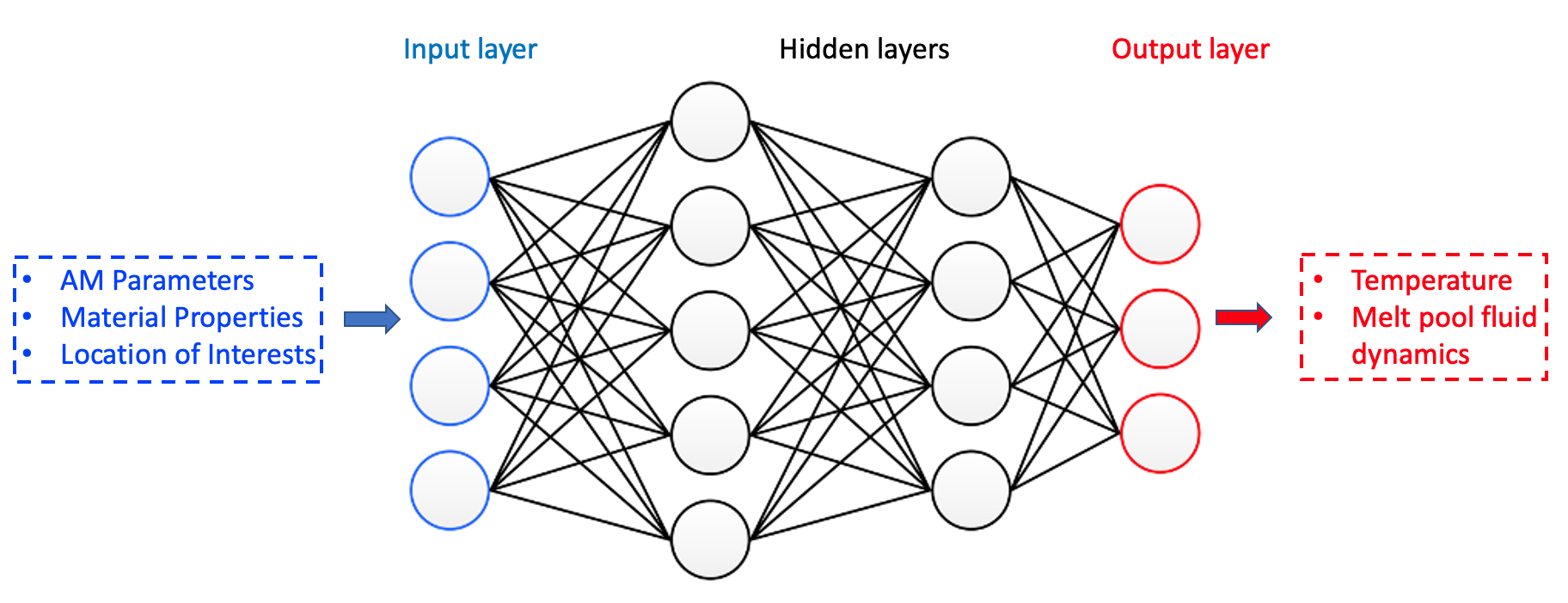
Figure 1: A fully connected deep neural network for metal AM.

where $\textbf{w}_{l}$ and $\textbf{b}_{l}$ are the weight matrix and bias vector of this layer, respectively. $\sigma_{l}$ is the activation function that can introduce the non-linearity to the system [69]. Widely used activation functions in deep learning are tanh function, Rectified linear unit (Relu), sigmoid function [70]. In this paper, we employ a swish activation function [71], which is a smoothed version of Relu function, defined as

$$\sigma(x)=swish(x)=x\ sigmoid(x)=x/(1-e^{-x})$$ (15)

The goal of the neural network is to learn the following mapping for a given set of manufacturing parameters (e.g,. alloy properties, laser power, and scanning speed):

$$[t,\bm{x}]\xrightarrow[]{\bm{W},\bm{b}}[\bm{u}_{NN},p_{NN},T_{NN}]$$ (16)

where the input $[t,\bm{x}]$ are the collocation points (in both space and time) of interest. The output $\bm{u}_{NN},p_{NN},T_{NN}$ are the velocity, pressure, and temperature fields we want to predict. To enable such a mapping, the hidden parameters of the neural network, $\bm{W}$ and $\bm{b}$, need to be identified by optimizing a meticulously designed loss function, which will be given in the next section. Once $\bm{W}$, and $\bm{b}$ are determined, the output prediction can be easily achieved by a feed-forward evaluation, which is very efficient since only a few matrix multiplications are needed in Eq. 14.

2.2.1 Loss function design

The loss function, $L(\bm{W},\bm{b})$, in the PINN for thermal-fluid flows consists of two components: $L_{data}(\bm{W},\bm{b})$ and $L_{pde}(\bm{W},\bm{b})$, which represents the constraint of matching existing labeled data and the constraints of satisfying fundamental physical principles. Their definitions are given as follows.

Let $\hat{\bm{u}}$, $\hat{p}$, and $\hat{T}$ denote the available labeled data for velocity, pressure, and temperature, respectively. These labeled data can be either obtained by experiments or validated high-fidelity simulations. As a mean squared deviation (MSD) of the discrepancy between the prediction and labeled data, the component in the loss function from the data constraint, $L_{data}$, is defined as

$$L_{data}(\bm{W},\bm{b})=\frac{1}{N_{u}}\sum_{i=1}^{N_{u}}\left[{\bm{u}_{NN}}(\bm{x}_{i},t_{i},\bm{W},\bm{b})-\hat{\bm{u}}(\bm{x}_{i},t_{i})\right]^{2}$$ (17)

$$+\frac{1}{N_{p}}\sum_{i=1}^{N_{p}}\left[{p}_{NN}(\bm{x}_{i},t_{i},\bm{W},\bm{b})-\hat{p}(\bm{x}_{i},t_{i})\right]^{2}$$

$$+\frac{1}{N_{T}}\sum_{i=1}^{N_{T}}\left[{T}_{NN}(\bm{x}_{i},t_{i},\bm{W},\bm{b})-\hat{T}(\bm{x}_{i},t_{i})\right]^{2}$$

where $N_{u}$, $N_{p}$, and $N_{T}$ are the number of labeled velocity, pressure, and temperature data points, respectively. Conventional off-the-shelf machine learning tools purely minimize this loss function to identify the hidden parameters. The success of this approach requires a massive amount of data-sets. However, considering the cost of experimental measurements and high-fidelity simulations, these labeled velocity, pressure, and temperature data points are expensive (sometimes impossible) to obtain. This limitation hinders the direct application of big-data based machine learning tools to metal AM process prediction.

To alleviate the dependence on big-data, we substitute extra expertise in fundamental physical principles into the loss function. These physical principles, often expressed as a set of PDEs with appropriate initial and boundary conditions, are highly condensed knowledge of fundamental physical mechanisms that can inform the neural network. For that, we first define the following residuals of conversation equations of momentum, mass, and energy (corresponding to Eqs.(1-3)) as

$$\left\{\begin{array}[]{ll}&\bm{r}_{M}:=\rho({\bm{u}}_{,t}+\bm{u}\cdot\nabla\textbf{u}-\bm{g})+\nabla p-2\mu\Delta\bm{u}\\ &{r}_{C}:=\nabla\cdot\bm{u}\\ &{r}_{T}:=(\rho c_{p}T)_{,t}+\bm{u}\cdot\nabla(\rho c_{p}T)+(\rho Lf_{L})_{,t}+\bm{u}\cdot(\rho L\nabla f_{L})-\kappa\nabla^{2}T-Q_{T}\end{array}\right.$$ (21)

To have well-posed systems, appropriate initial and boundary conditions are often necessary. In this paper, the initial boundary conditions are treated as part of the labeled data constraint. For boundary conditions (BCs), many existing PINN frameworks utilize a “soft” approach by designing additional loss components defined on the collocation points of boundaries to constrain the BCs. The downsides of this approach are two-fold: (1) The accuracy of satisfying the BCs is not guaranteed ; (2) The assigned weight of BC loss can affect learning efficiency, and no theory is existed to guide choosing the weight at this point.

In this paper, we treat the Dirichlet BC in a “hard” way by using a particular portion of the neural network to purely satisfy the prescribed Dirichlet BC. For that, we first define a Heaviside function as

$$H_{\epsilon}(\bm{x})=\left\{\begin{aligned} &1-cos[d(\bm{x})\pi/\epsilon]&\text{if}\quad d(\bm{x})&<&\epsilon\\ &{\quad\quad\quad\quad}1&\quad\text{ if}\quad d(\bm{x})\ &\geq&\epsilon\end{aligned}\right.$$ (22)

where $d(\bm{x})$ is the distance to the Dirichlet boundary. $\epsilon$ defines a artificial thickness of the boundary. With $H_{\epsilon}(\bm{x})$, the predictions of the neural networks are defined as

$$\bm{u}_{NN}=\bm{u}_{bc}[1-H_{\epsilon}(\bm{x})]+\bm{u}H_{\epsilon}(\bm{x})$$ (23)

$$p_{NN}=p_{bc}[1-H_{\epsilon}(\bm{x})]+pH_{\epsilon}(\bm{x})$$ (24)

$$T_{NN}=T_{bc}[1-H_{\epsilon}(\bm{x})]+TH_{\epsilon}(\bm{x})$$ (25)

where $\bm{u}_{bc}$, $p_{bc}$, and $T_{bc}$ are the prescribed velocity, pressure, and temperature. $\bm{u}$, $p$, and $T$ are the solutions that satisfy the PDEs in the interior. Since $H_{\epsilon}(\bm{x})$ smoothly changes from 1 to 0 as $d(\bm{x})$ approaches to 0, the prediction will automatically satisfy the prescribed values by definition, without needing additional constraint. Then, the loss term from the PDEs with embedded Dirichlet BCs is defined as.

$$L_{pde}^{1}(\bm{W},\bm{b})=\frac{1}{N_{r1}}\sum_{i=1}^{N_{r1}}\bm{r}_{M}[{\bm{u}_{NN}}(\bm{x}_{i},t_{i},\bm{W},\bm{b}),{p}_{NN}(\bm{x}_{i},t_{i},\bm{W},\bm{b}),{T}_{NN}(\bm{x}_{i},t_{i},\bm{W},\bm{b}))]^{2}$$ (26)

$$+\frac{1}{N_{r1}}\sum_{i=1}^{N_{r1}}{r}_{C}[{\bm{u}_{NN}}(\bm{x}_{i},t_{i},\bm{W},\bm{b}),{p}_{NN}(\bm{x}_{i},t_{i},\bm{W},\bm{b}),{T}_{NN}(\bm{x}_{i},t_{i},\bm{W},\bm{b}))]^{2}$$

$$+\frac{1}{N_{r1}}\sum_{i=1}^{N_{r1}}{r}_{T}[{\bm{u}_{NN}}(\bm{x}_{i},t_{i},\bm{W},\bm{b}),{p}_{NN}(\bm{x}_{i},t_{i},\bm{W},\bm{b}),{T}_{NN}(\bm{x}_{i},t_{i},\bm{W},\bm{b}))]^{2}$$

where $N_{r1}$ denotes the number of collocation points to constrain the PDEs.

In the thermal-fluid flow model for metal AM processes, Neumann BCs incorporate surface tension for flow field and laser for thermal field. In this paper, the Neumann BCs are handled by the conventional way, where the following term is added in the loss function

$$L_{pde}^{2}(\bm{W},\bm{b})=\frac{1}{N_{r2}}\sum_{i=1}^{N_{r2}}\left\{2\mu\nabla^{S}{\bm{u}_{NN}}(\bm{x}_{i},t_{i},\bm{W},\bm{b})\cdot\bm{n}-{p}_{NN}(\bm{x}_{i},t_{i},\bm{W},\bm{b})\bm{n}-\bm{\tau}(\bm{x}_{i},t_{i})\right\}^{2}$$ (27)

$$+\frac{1}{N_{r3}}\sum_{i=1}^{N_{r3}}[\kappa\nabla{{T}_{NN}}(\bm{x}_{i},t_{i},\bm{W},\bm{b})\cdot\bm{n}-{q}(\bm{x}_{i},t_{i})]^{2}$$

where $N_{r2}$ and $N_{r3}$ denote the number of collocation points on the fluid and temperature Neumann boundaries, respectively.

With above definitions, The hidden parameters $\bm{W}$ and $\bm{b}$ are obtained by minimizing the following total loss function, which are a linear combination of data constraint of $L_{data}$ and PDE constraints of $L_{pde}^{1}$ and $L_{pde}^{2}$.

$$\displaystyle\min_{\bm{W},\bm{b}}L(\bm{W},\bm{b})=(1-\lambda_{pde}^{1}-\lambda_{pde}^{2})L_{data}(\bm{W},\bm{b})+\lambda_{pde}^{1}L_{pde}^{1}(\bm{W},\bm{b})+\lambda_{pde}^{2}L_{pde}^{2}(\bm{W},\bm{b})$$ (28)

$\lambda_{pde}^{1}$ and $\lambda_{pde}^{2}$ are two positive numbers between 0 and 1, which define the weight of the physical law constraints in the loss function.

2.2.2 Learning procedure

The PINN model is trained by minimizing the loss function defined in Eq. 28. Most of current machine learning frameworks solve the optimization problem by a stochastic gradient descent (SGD) algorithm, which is a stochastic approximation of the gradient descent (GD) optimization [72]. SGD only uses a subset of collocation points, randomly sampled from the input space at each iteration, to calculate the directional gradient. Research shows that SGD works very well to skip bad local minima. One issue with SGD is the oscillation of gradient direction caused by the random selection of sampled collocation points. In this paper, the Adam method [73] that combines adaptive learning rate and momentum methods is used to improve convergence speed [73].

The PINN learning process needs the spatial and temporal derivatives of $\bm{u}$, $p$, and $T$, which can be accurately and efficiently calculated by using automatic differentiation (AD) [74]. The basic idea of AD is to use the chain rule to back-propagate derivatives from the output layer to the input layer since the connection between layers of a neural network is analytically defined. Compared to numerical differentiation techniques (e.g., finite difference and finite element), AD does not suffer from truncation or round-off errors, resulting in much higher accuracy. AD has been gaining increasing attention in the machine learning community and has been implemented in many modern deep learning frameworks, such as TensorFlow [39], PyTorch [40], Theano [41], and Caffe [42]. In this paper, the PINN formulation is implemented in TensorFlow.

3 Applications

3.1 Solidification of aluminum in a graphite mold without labeled data

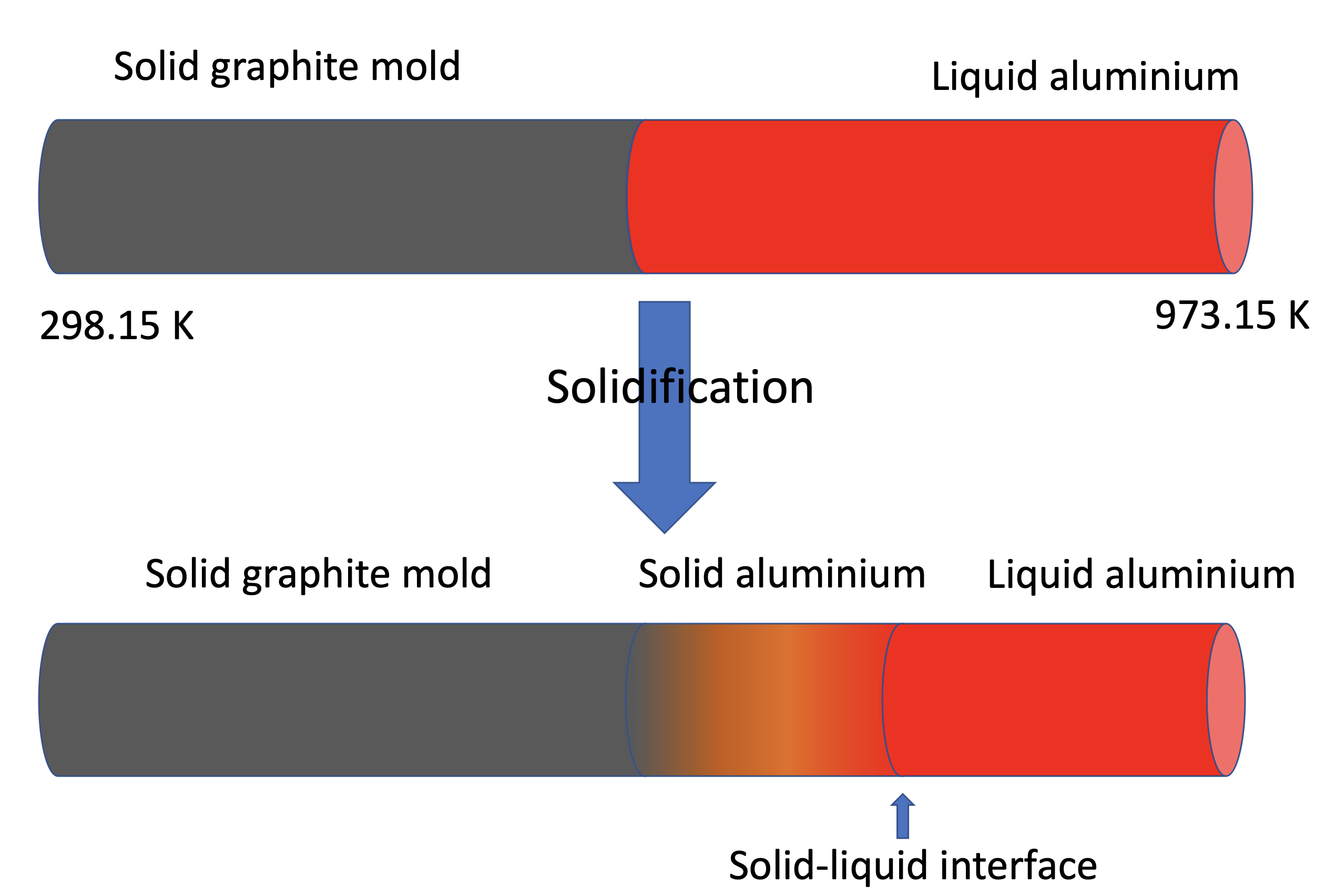
Figure 2: 1D solidificaton process from [56]

The solidification process of aluminum in a graphite mold from the textbook Solidification by Dantzig and Rappaz [56] is investigated to assess the performance of the PINN formulation. Only thermodynamics with phase transition is considered in the simulations here. Figure 2 shows the problem setup, where the left half of the domain (-0.4 m $\leq x\leq$ 0.0 m) is occupied by a solid graphite mold with temperature $T_{low}$ = 298.15 K, and the right half of the domain (0.0 m $<x\leq$ 0.4 m) is occupied with liquid aluminum with temperature $T_{high}$ = 973.15 K, which is higher than the melting temperature of aluminum $T_{melt}=933.15K$. As depicted in Figure 2 (lower), solidification occurs by transferring heat from the aluminum into the mold, and the solid-liquid interface propagates towards the right end. The material properties of the graphite mold and aluminum are given in Table 1. The analytical solutions have been derived in [56] for this problem and are specified as follows.

Table 1: Definition of material properties for the solidification problem

Materials	Graphite	Aluminum (solid)	Aluminum (liquid)
Density ($kg/m^{3}$)	2200	2555	2555
Specific heat ($J/(kg\ K)$)	1700	1190	1190
Thermal conductivity ($W/(kg\ K)$)	100	211	91
Latent heat ($J/kg$)	-	$398000$	-

$$x^{*}=7.095\times 10^{-3}\sqrt{t}\ s$$ (29)

$$T_{m}=769.95+471.8erf(\frac{96.69x}{\sqrt{t}})\ K$$ (30)

$$T_{s}=769.95+360.2erf(\frac{60.02x}{\sqrt{t}})\ K$$ (31)

$$T_{l}=973.15-111.4erfc(\frac{91.39x}{\sqrt{t}})\ K$$ (32)

where $x^{*}$ is the location of solid-liquid interface over time, $T_{m}$, $T_{s}$, and $T_{l}$ are the temperature distribution in the mold, solid aluminum, and liquid aluminum, respectively.

Despite the simplicity, solving this problem provides valuable insights into the solidification behavior and the performance of the machine learning model. The PINN model employs 5 hidden layers and 200 neurons of each layer, which provides better results over others based on our non-exhaustive investigation. The neural network is physically informed with the energy conservation principle defined in Eq. 3 and trained without labeled data-set. The PINN model predicts the temperature distribution from $t$ = 5 s to $t$ = 10 s.

Figure 3 illustrates the PINN setup and the resulting temperature prediction in the space-time (${x}-t$) slab for the solidification process. We compare the performance of the proposed “hard” approach with the conventional “soft” approach for the Dirichlet boundary condition in Figure 4, which depicts the learning process and temperature predictions at 10 s. The plot shows that the “hard” approach can not only facilitate the learning process (see Figure 4 (left)) but also produce more accurate temperature prediction (see Figure 4 (right)).

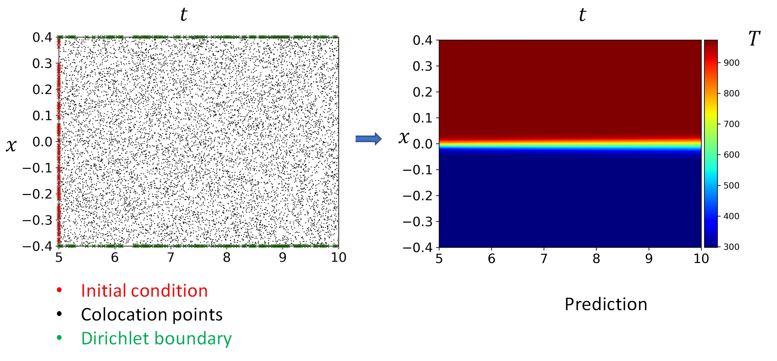
Figure 3: PINN model for the solidification problem. Left: PINN setup. Right: Temperature prediction.

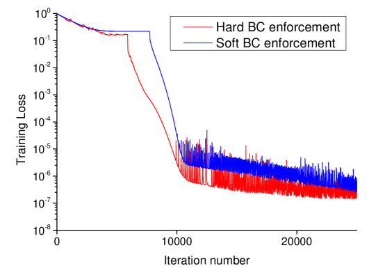
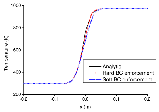
Figure 4: Comparison between “hard” BC and “soft” BC. Left: learning speed. Right: The temperature distribution at 10 s.

One important question is how does the PINN’s predictive capability compare with traditional numerical methods, such as finite element method (FEM). To answer this question, we simulate this solidification problem by using PINN with four different numbers of collocation points and linear FEM with four equivalent resolutions ($N_{x}$= 50, 100, 150, and 200 along $x$ direction). Figure 5 shows the predictions of PINN and FEM for the time history of solid-liquid interface position with the four resolutions. The convergence rate of error of temperature prediction over the ${x}-t$ slab is shown in Figure 6. The two plots indicate that PINN and FEM obtain similar convergence rates. However, when the resolution is low, the PINN still attains high accuracy while noticeable discrepancy is observed for the standard FEM.

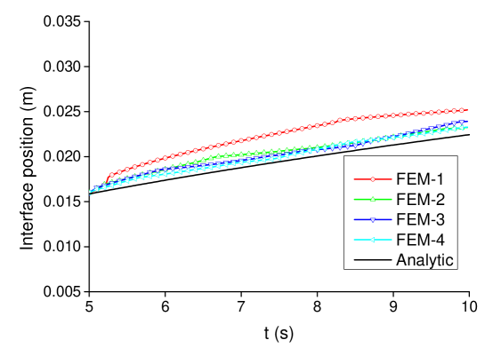
Figure 5: Predicted time history of solid-liquid interface position. Left: refinement study of FEM. Right: refinement study of PINN.

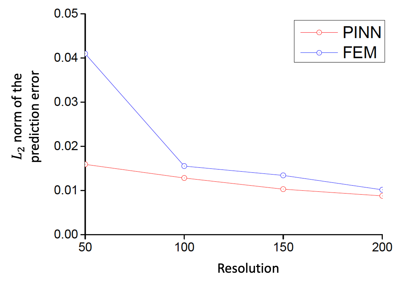
Figure 6: $L_{2}$ norm of prediction error of PINN and FEM with different resolutions.

3.2 NIST AM-bench test series

In this section, we apply the PINN framework to the Additive Manufacturing Benchmark (AM-Bench) test series conducted by the National Institute of Standards and Technology (NIST) [75, 76]. In 2018, NIST performed a series of metal AM experiments with different manufacturing parameters, which attracted blind simulations to compare with the in-situ and ex-situ measurements, such as temperature, melt pool dimensions and micro-structures [75]. The archived experimental measurements provide valuable benchmark data for modelers to test the predictive capabilities of simulation models. In this paper, we use the proposed PINN framework to predict the temperature, melt pool fluid dynamics, melt pool dimensions, and cooling rates during the NIST AM processes, which corresponds to the first challenge in the NIST AM-Bench test series [76]. To the best knowledge of the authors, this is the first application of PINN to three dimensional metal AM processes modeling.

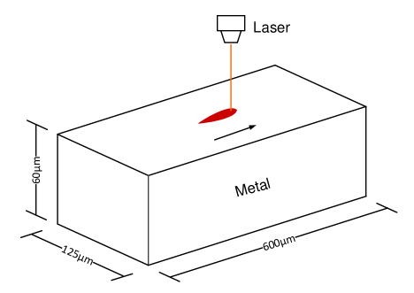
Figure 7: NIST AM-bench test series

Figure 7 shows a schematic description of the NIST AM-Bench test, a selective laser beam melting process of a pure Inconel 625 (IN625) substrate. The material properties used in this paper are summarized in Table 2. The laser is applied by imposing the following moving heat flux on the substrate.

$$\kappa\nabla{T}\cdot\bm{n}=q_{laser}=\frac{2Q\eta}{\pi r_{b}^{2}}exp(\frac{-2((x-V_{s}t)^{2}+y^{2})}{r_{b}^{2}})$$ (33)

where $Q$ is the laser power, $\eta$ is the absorptivity, $r_{b}$ is the laser beam radius, $V_{s}$ is the laser scanning speed. $\eta=0.43$ and $r_{b}=50$ $\mu$m are used in this paper. Table 3 lists the laser power and scanning speed of three cases used in the NIST experiments. Based on the fact that the top surface deformation is relatively small compared with the melt pool dimension, a flat top surface is assumed, and the following boundary condition is applied for the fluid field.

$$-p\bm{n}+2\mu\nabla^{s}\bm{u}\cdot\bm{n}=\bm{\tau}=\frac{d\sigma}{dT}[\nabla T-(\nabla T\cdot\bm{n})\bm{n}]$$ (34)

where $\frac{d\sigma}{dT}$ is the Marangoni coefficient, which is only effective in the tangential direction of the temperature gradient. Except for the top surface, no-slip and fixed reference temperature boundary conditions are used for other surfaces.

The PINN model employs a fully connected neural network with 5 hidden layers and 250 neurons per layer, which provides a better balance of accuracy and training efficiency over others based on our non-exhaustive investigation. The model is physically informed by the conservation laws of momentum, mass, and energy defined in Eqs. 1- 3. A total of $788,651$ collocation points in the $\bm{x}-t$ slab are used to penalize the PDE residuals (see Eq. 21) in the loss function. Due to the limited point-wise measurements provided by NIST, we use high-fidelity finite element thermal-fluid simulations to generate the labeled data-sets to facilitate the training. The simulated results are treated as “ground truth” after being compared with the NIST experimental measurements. Appendix briefly presents the core formulation of the finite element formulation that has also been validated for other metal manufacturing process modeling [30]. The setup for FEM simulations, such as time step and mesh size, is also specified in Appendix. The FEM simulations have been run up to 2.0 ms for all the three cases listed in Table 3, but only a small portion of the simulated data between 1.2 ms and 1.5 ms is used as labeled training data in the PINN model, which then predicts the manufacturing processes for a wider time interval from 0 ms to 2.0 ms.

Table 2: Mechanical properties of IN625

Name	Property	Value
Density	$\rho(kg\cdot m^{-3})$	$8440$
Solidus temperature	$T_{s}(K)$	$1563$
Liquid temperature	$T_{l}(K)$	$1623$
Solid specific heat capacity	$c_{ps}(J\cdot kg^{-1}\cdot K^{-1})$	$0.2441T+338.39$
Liquid specific heat capacity	$c_{pl}(J\cdot kg^{-1}\cdot K^{-1})$	$709.25$
Solid solid conductivity	$\kappa_{s}(W\cdot m^{-1}\cdot K^{-1})$	$3.0\times 10^{-5}T^{2}-0.0366T+18.588$
Liquid solid conductivity	$\kappa_{l}(W\cdot m^{-1}\cdot K^{-1})$	$30.078$
Latent heat of fusion	$c_{L}(KJ\cdot kg^{-1}\cdot K^{-1})$	$290$
Dynamic viscosity	$\mu(Pa\cdot s)$	$7\times 10^{-3}$
Marangoni coefficient	$\frac{\partial\gamma}{\partial T}(N\cdot m^{-1}\cdot K^{-1})$	$-2\times 10^{-5}$
Reference temperature	$T_{ref}(K)$	$295$

Table 3: Three laser parameters

Parameters	Case A	Case B	Case C
Laser Power	150 W	195 W	195 W
Scan Speed	0.4 m/s	0.8 m/s	1.2 m/s

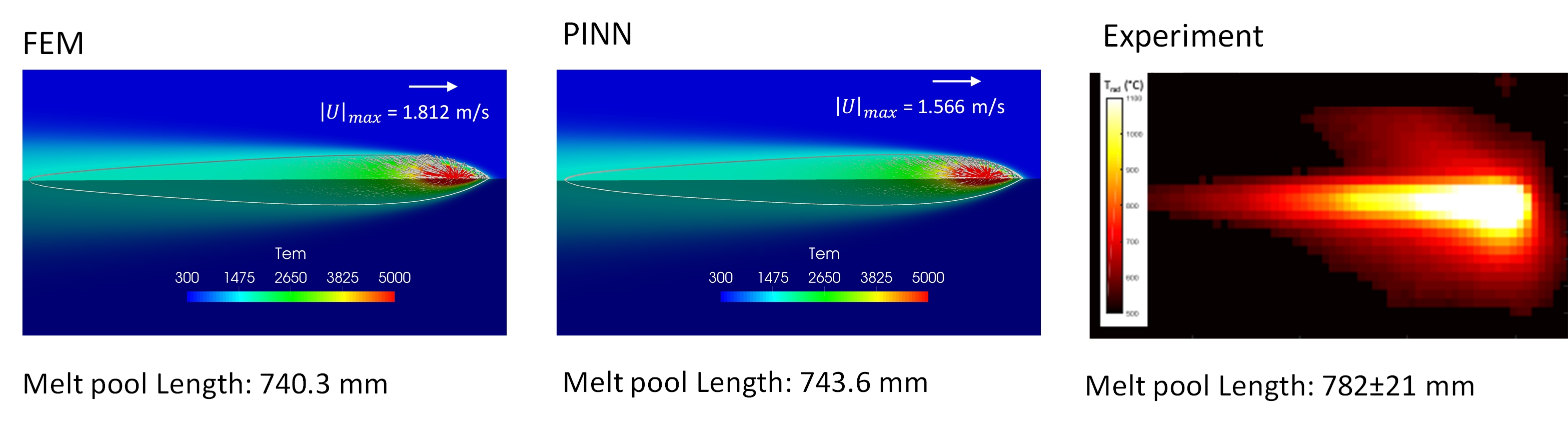
Figure 8: Comparison of the predictions of the temperature and melt pool fluid dynamics of FEM, PINN and experiment for case B (195 W, 0.8 m/s) at quasi-steady state (2 ms), when the melt pool shape is not changing. Left: FEM prediction. Middle: PINN prediction. Right: Thermal video frame based on radiance temperature.

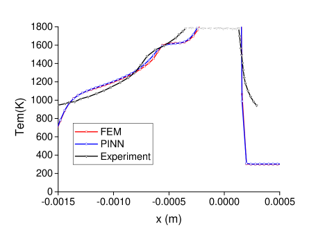
Figure 9: Temperature profile along the scan track for case B (195 W, 0.8 m/s) at quasi-steady state. Experimental data extracted from NIST AM-Bench test series [77] are also plotted for comparison.

We first compare the predicted results of FEM and PINN with available experimental data for case B (195 W, 0.8 m/s). The purpose is two-fold: 1) Ensure the credibility of FEM data as the training data; 2) Validate the PINN model. Figure 8 shows the temperature field, melt pool fluid dynamics, and melt pool shape at 2.0 ms. The fast-moving laser, along with the effect of a negative Marangoni coefficient that drives the liquid metal from higher temperature to lower temperature, leading to a long and shallow melt pool. The predicted temperature profile along the scan track and experimental measurement extracted from [77] is plotted in Figure 9 for comparison. The predicted results by both FEM and PINN show good agreement with available experimental data. Figure 8 and Figure 9 also show that the PINN model, with a moderate amount of training data, can generate very similar predictions of temperature, melt pool length, and melt pool fluid velocity to those of FEM.

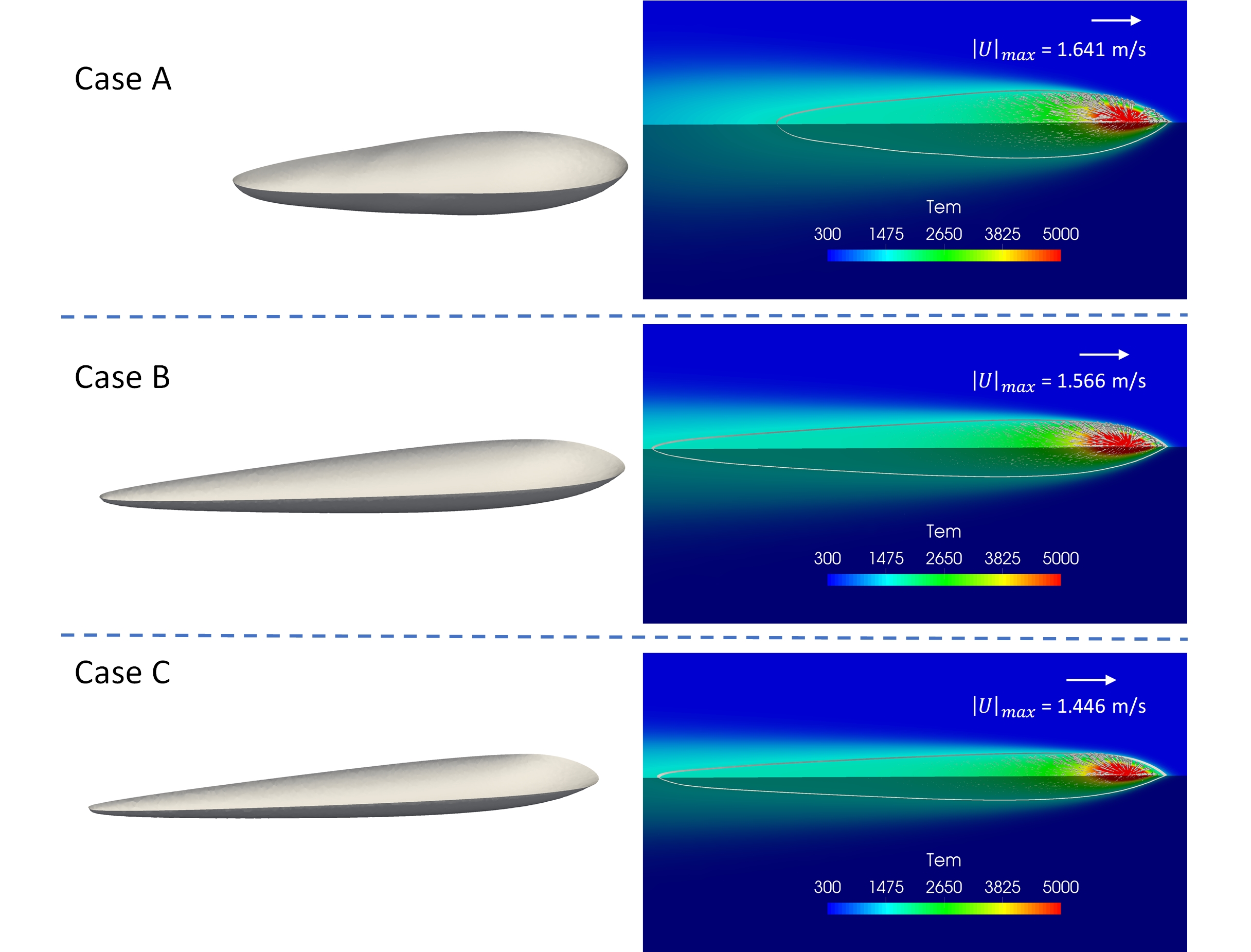
Figure 10: Melt pool shape and melt pool flow velocity predicted by PINN for case A, B and C at quasi-steady state (2 ms).

Table 4: Melt pool dimensions of case A, B and C.

Cases	Approaches	Length ($\mu m$)	Width ($\mu m$)	Depth ($\mu m$)
Case A	PINN	594.8 (9.7%)	193.3	64.0
	FEM	584.4 (11.3%)	190.8	62.8
	Gan et al. [32]	542 (17.8%)	-	-
	Experiment [77]	$659\pm 21$	-	-
Case B	PINN	740.3 (5.1%)	160.0	52.8
	FEM	743.6 (4.7%)	157.5	52.5
	Gan et al. [32]	843 (8.1%)	-	-
	Experiment [77]	$782\pm 21$	-	-
Case C	PINN	732.5 (2.9%)	131.5	43.2
	FEM	727.2 (3.6%)	130.3	42.6
	Gan et al. [32]	785 (4.1%)	-	-
	Experiment [77]	$754\pm 46$	-	-

We then apply the PINN model to all the three cases listed in Table 3. The predicted melt pool shape and the fluid velocity field within the melt pool are presented in Figure 10. The laser results in sufficiently high velocity in the melt pool, which reaches up to 1.641 m/s, 1.566 m/s, and 1.446 m/s for the case A, B, and C, respectively. The predicted melt pool dimensions compared with the present FEM results, the thermal-fluid simulation results by Gan et al. [32] that won an award in the NIST AM-bench competition, and available NIST experimental measurements are listed in Table 4. For melt pool length, the relative discrepancy (with respect to the mean NIST experimental measurements) of PINN, FEM and Gan’s predictions are 9.7 $\%$, 11.3 $\%$ and 17.8 $\%$ for case A, 5.1 $\%$, 4.7 $\%$ and 8.1 $\%$ for case B, and 2.9 $\%$, 3.6 $\%$ and 4.1 $\%$ for case C. Similar accuracy is observed among these approaches. Based on the model predictions, we notice that case A generates the smallest melt pool length but the biggest width and depth, which could be due to the low scanning speed that gives the laser more time to melt the underneath metal. In contrast, case B and C have a slightly bigger laser power but much faster scanning speeds, which consequently result in longer melt pool lengths but smaller widths and depths. Between case B and case C with the same laser power, lower spanning (case B) speed results in bigger melt pool dimensions in all directions.

A critical factor in metal AM is the cooling rate, which profoundly influences dendrite arm spacing, grain structure, micro-segregation, and hot cracking. In this paper, the cooling rate is calculated as

$$R_{c}=\frac{T_{s}-1273.15K}{t_{c}}$$ (35)

where $t_{c}=({D_{s}-D_{1273.15}})/{V_{s}}$, the cooling time interval determined by dividing the distance between solidus temperature and 1273.15 K by the scanning speed $V_{s}$.

Table 5: Cooling rates of case A, B and C.

Cases	Approaches	solid cooling rate ($K/s$)
Case A	PINN	$8.54\times 10^{5}$ (37.7%)
	FEM	$8.00\times 10^{5}$ (29.0%)
	Gan et al. [32]	$5.11\times 10^{5}$ (17.6%)
	Experiment [77]	$6.20\times 10^{5}\pm 7.99\times 10^{4}$
Case B	PINN	$8.59\times 10^{5}$ (8.1%)
	FEM	$8.16\times 10^{5}$ (12.7%)
	Gan et al. [32]	$6.89\times 10^{5}$ (26.3%)
	Experiment [77]	$9.35\times 10^{5}\pm 1.43\times 10^{5}$
Case C	PINN	$1.38\times 10^{6}$ (7.8%)
	FEM	$1.38\times 10^{6}$ (7.8%)
	Gan et al. [32]	$11.30\times 10^{5}$ (11.7%)
	Experiment [77]	$1.28\times 10^{6}\pm 3.94\times 10^{5}$

Table 5 presents the PINN prediction of cooling rate $R_{c}$ for the case A, B, and C. The results of FEM, Gan’s results and experimental measurements are also listed for comparison. Both modeling and experiment show that cooling rate increases from case A to case C. For the cooling rate, the relative discrepancy (with respect to the mean NIST measurements) of PINN, FEM and Gan’s predictions are 37.7 $\%$, 29.0 $\%$ and 17.6 $\%$ for case A, 8.1 $\%$, 12.7 $\%$ and 26.3 $\%$ for case B, and 7.8 $\%$, 7.8 $\%$ and 11.7 $\%$ for case C. Although all the models’ prediction accuracy becomes lower compared with melt pool dimension prediction, we notice that the NIST measurements in cooling rates also exhibit significantly higher fluctuations than melt pool dimension measurements. If using this discrepancy as an accuracy metric, the proposed PINN model only underperforms in case A and outperforms in both case B and case C, which is advantageous compared with the other two high-fidelity FEM simulations that employ millions of elements.

4 Conclusion

This paper presents the first attempt of using the physics-informed neural network (PINN) to predict the temperature and melt pool fluid dynamics in metal AM processes. We applied the PINN model to two representative metal manufacturing problems. The results show that the PINN can accurately predict the quantities of interest by only using a small amount of labeled training data. This paper is also the first few applications of scientific machine learning (SciML), currently confined to single-phase systems, to complex multi-scale and multi-physics problems that involve multi-phase fluid dynamics, heat transfer and phase transition. The two major technical contributions relevant to metal AM of the paper are:

• A SciML framework for metal AM processes, which can accurately predict temperature, pressure, and velocity field without relying on big-data.

• A “hard” approach for imposing Dirichlet boundary condition, which exactly imposes the prescribed value and speeds up the learning process.

Although deep learning models cannot replace conventional numerical tools that will continue to be the principal player, the initial success presented in this paper demonstrates PINN’s potential on the modeling and prediction of complicated metal AM processes and paves the way for the broad adoption in advanced manufacturing.

We also have to admit that this paper does not comprehensively handle the complexity of metal AM processes. To be precise, the PINN model here does not resolve the ambient gas phase, free-surface deformation of the melt pool, and the evaporation phenomenon, although the effects are not crucial for the applications considered in the paper. In the future, the multi-phase Navier-Stokes will be enhanced with the evaporation model in the momentum equations, which was used in our control volume finite element model [14], to capture the heat loss, composition change, and fluid motion induced by evaporation. Additional PDEs, such as convection equation of level set or volume-of-fluid used in the previous works [30, 23], will be incorporated into the PINN to enable modeling metal AM process at the powder scale.

5 Acknowledgement

J. Yan is partially supported by ASME Robert M. and Mary Haythornthwaite Research Initiation Award and Singapore National Research Foundation (NRF2018-ITS004-0011). The PINN models were trained at the Texas Advanced Computing Center (Tacc) through a startup allocation on Frontera (CTS20014). These supports are greatly acknowledged.

6 Appendix: High-fidelity FEM thermal-fluid simulations

The high-fidelity FEM thermal-fluid simulations make use of a residual-based variational multi-scale formulation (VMS) based on our previous work in [30]. The core formulation is briefly presented as follows. Let $\mathcal{W}$ denote the testing function space for the Navier-Stokes and energy conversation equations, $\mathcal{V}$ denote the unknown velocity $\bm{u}$, pressure $p$, and temperature $T$ fields. The RBVMS formulation of thermal-fluid flows is stated as: $\forall\{\mathbf{w},q,\eta\}\in\mathcal{W}$, find $\{\mathbf{u},p,T\}\in\mathcal{V}$, such that

$$\int_{\Omega}\mathbf{w}\cdot\rho\left(\mathbf{u}_{,t}+\bm{u}\cdot\nabla\bm{u}-\mathbf{g}\right)d\Omega+\int_{\Omega}p\nabla\cdot\mathbf{w}d\Omega$$

$$-\int_{\mathbf{\Gamma}}\mathbf{w}\cdot\mathbf{h}d\Gamma+\int_{\Omega}\nabla^{s}\mathbf{w}:\mu\nabla^{s}\bm{u}d\Omega+\int_{\Omega}q\nabla\cdot\bm{u}d\Omega$$

$$+\int_{\Omega}\eta\left[(\rho c_{p}T)_{,t}+\bm{u}\cdot\nabla(\rho c_{p}T)+(\rho Lf_{L})_{,t}+\bm{u}\cdot\nabla(\rho Lf_{L})\right]d\Omega+\int_{\Omega}\nabla\eta\cdot\kappa\nabla{T}d\Omega-\int_{\Omega}\eta Q_{T}d\Omega$$

$$+\Sigma_{e=1}^{n_{el}}\int_{\Omega^{e}}\tau_{M}(\bm{u}\cdot\nabla\mathbf{w}+\frac{\nabla{q}}{\rho})\cdot\mathbf{r}_{M}d\Omega+\Sigma_{e=1}^{n_{el}}\int_{\Omega^{e}}\rho\tau_{C}\nabla\cdot\mathbf{w}r_{C}d\Omega$$

$$-\Sigma_{e=1}^{n_{el}}\int_{\Omega^{e}}\tau_{M}\mathbf{w}\cdot\left[\mathbf{r}_{M}\cdot\nabla\bm{u}\right]d\Omega-\Sigma_{e=1}^{n_{el}}\int_{\Omega^{e}}\frac{\nabla\mathbf{w}}{\rho}:(\tau_{M}\mathbf{r}_{M}\otimes\tau_{M}\mathbf{r}_{M})d\Omega$$

$$+\Sigma_{e=1}^{n_{el}}\int_{\Omega^{e}}\tau_{T}(\bm{u}\cdot\nabla\eta)r_{T}d\Omega=0$$ (36)

where $\mathbf{r}_{M}$, ${r}_{C}$ and ${r}_{T}$ are the residuals of momentum, continuity, and energy conservation equations (Eq. 21). $\tau_{M}$, $\tau_{C}$ and $\tau_{T}$ are the corresponding stabilization parameters [30]. Other widely used stabilization parameters can be found in [78, 79, 80, 81, 79, 80]. The VMS and its extensions on moving fluid domains using Arbitrary Lagrangian-Eulerian technique (ALE-VMS) [82, 83] and Space-Time (ST-VMS) technique [84, 85, 86, 87, 88] have been used as high-fidelity models to simulate a set of challenging fluid dynamics and fluid-structure interaction problems [89]. Several recent applications include environmental flows [90], wind energy [91, 92, 93, 85, 94, 95, 96, 97, 98, 99], tidal energy [100, 101, 102], bio-mechanics [103, 104], and transportation engineering [105].

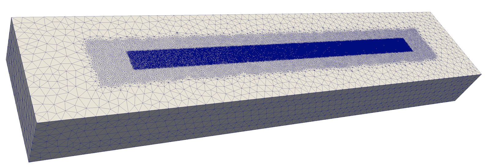
Figure 11: The mesh employed in the high-fidelity FEM thermal-fluid simulations.

The FEM simulations of the NIST AM-bench test series make use of a mesh with 4,464,276 tetrahedral elements. A local refinement is designed to capture the moving laser, which is shown in Figure 11. The unknown velocity, pressure, and temperature are solved in a fully coupled fashion. Generalized-$\alpha$ is used for time integration with $\Delta t=1\times 10^{-6}$ s. The nonlinear equations are linearized by Newton’s method. The resulting linear systems are solved by GMRES with block preconditioning [106]. These simulations are executed at Stampede2 at Texas Advanced Computing Center (TACC) with 192 CPU processors.

References

- [1] C. Zhao, K. Fezzaa, R. Cunningham, H. Wen, F. De Carlo, L. Chen, A. Rollett, T. Sun, Real-time monitoring of laser powder bed fusion process using high-speed x-ray imaging and diffraction, Scientific reports 7 (1) (2017) 1–11.
- [2] R. Cunningham, C. Zhao, N. Parab, C. Kantzos, J. Pauza, K. Fezzaa, T. Sun, A. Rollett, Keyhole threshold and morphology in laser melting revealed by ultrahigh-speed x-ray imaging, Science 363 (6429) (2019) 849–852.
- [3] Q. Guo, C. Zhao, M. Qu, L. Xiong, S. Hojjatzadeh, L. Escano, N. Parab, K. Fezzaa, T. Sun, L. Chen, In-situ full-field mapping of melt flow dynamics in laser metal additive manufacturing, Additive Manufacturing 31 (2020) 100939.
- [4] NIST Additive Manufacturing Benchmark Test Series (AM-BENCH), https://www.nist.gov/ambench, accessed: 2020-03-08 (2020).
- [5] AFRL Additive Manufacturing Modeling Challenge Series, https://www.americamakes.us/america-makes-and-afrl-announce-am-modeling-challenge/, accessed: 2020-07-07 (2020).
- [6] C. Noble, A. Anderson, N. Barton, J. Bramwell, A. Capps, M. Chang, J. Chou, D. Dawson, E. Diana, T. Dunn, Ale3d: An arbitrary lagrangian-eulerian multi-physics code, Tech. rep., Lawrence Livermore National Lab.(LLNL), Livermore, CA (United States) (2017).
- [7] S. Khairallah, A. Anderson, A. Rubenchik, W. King, Laser powder-bed fusion additive manufacturing: Physics of complex melt flow and formation mechanisms of pores, spatter, and denudation zones, Acta Materialia 108 (2016) 36–45.
- [8] T. T. Roehling, S. S. Wu, S. A. Khairallah, J. D. Roehling, S. S. Soezeri, M. F. Crumb, M. J. Matthews, Modulating laser intensity profile ellipticity for microstructural control during metal additive manufacturing, Acta Materialia 128 (2017) 197–206.
- [9] S. Khairallah, A. Martin, J. Lee, G. Guss, N. Calta, J. Hammons, M. Nielsen, K. Chaput, E. Schwalbach, M. Shah, G. Chapman, T. Willey, A. Rubenchik, A. Anderson, Y. Wang, M. Matthews, W. King, Controlling interdependent meso-nanosecond dynamics and defect generation in metal 3d printing, Science 368 (6491) (2020) 660–665.
- [10] G. Knapp, T. Mukherjee, J. Zuback, H. Wei, T. Palmer, A. De, T. DebRoy, Building blocks for a digital twin of additive manufacturing, Acta Materialia 135 (2017) 390–399.
- [11] T. Mukherjee, H. Wei, A. De, T. DebRoy, Heat and fluid flow in additive manufacturing—part i: Modeling of powder bed fusion, Computational Materials Science 150 (2018) 304–313.
- [12] T. Mukherjee, H. Wei, A. De, T. DebRoy, Heat and fluid flow in additive manufacturing–part ii: Powder bed fusion of stainless steel, and titanium, nickel and aluminum base alloys, Computational Materials Science 150 (2018) 369–380.
- [13] S. Lin, Numerical methods and high performance computing for modeling metallic additive manufacturing processes at multiple scales, Ph.D. thesis, Northwestern University (2019).
- [14] S. Lin, Z. Gan, J. Yan, G. Wagner, A conservative level set method on unstructured meshes for modeling multiphase thermo-fluid flow in additive manufacturing processes, Computer Methods in Applied Mechanics and Engineering.
- [15] E. Attar, C. Körner, Lattice boltzmann model for thermal free surface flows with liquid–solid phase transition, International Journal of Heat and Fluid Flow 32 (1) (2011) 156–163.
- [16] C. Körner, E. Attar, P. Heinl, Mesoscopic simulation of selective beam melting processes, Journal of Materials Processing Technology 211 (6) (2011) 978–987.
- [17] C. Körner, A. Bauereiß, E. Attar, Fundamental consolidation mechanisms during selective beam melting of powders, Modelling and Simulation in Materials Science and Engineering 21 (8) (2013) 085011.
- [18] T. I. Zohdi, Additive particle deposition and selective laser processing-a computational manufacturing framework, Computational Mechanics 54 (1) (2014) 171–191.
- [19] T. Zohdi, A direct particle-based computational framework for electrically enhanced thermo-mechanical sintering of powdered materials, Mathematics and Mechanics of Solids 19 (1) (2014) 93–113.
- [20] R. Ganeriwala, T. I. Zohdi, Multiphysics modeling and simulation of selective laser sintering manufacturing processes, Procedia Cirp 14 (2014) 299–304.
- [21] W. Yan, W. Ge, Y. Qian, S. Lin, B. Zhou, W. K. Liu, F. Lin, G. J. Wagner, Multi-physics modeling of single/multiple-track defect mechanisms in electron beam selective melting, Acta Materialia 134 (2017) 324–333.
- [22] W. Yan, Y. Qian, W. Ge, S. Lin, W. K. Liu, F. Lin, G. J. Wagner, Meso-scale modeling of multiple-layer fabrication process in selective electron beam melting: inter-layer/track voids formation, Materials & Design 141 (2018) 210–219.
- [23] W. Yan, S. Lin, O. Kafka, Y. Lian, C. Yu, Z. Liu, J. Yan, S. Wolff, H. Wu, E. Ndip-Agbor, M. Mozaffar, K. Ehmann, J. Cao, G. Wagner, W. Liu, Data-driven multi-scale multi-physics models to derive process–structure–property relationships for additive manufacturing, Computational Mechanics 61 (5) (2018) 521–541.
- [24] W. Yan, W. Ge, J. Smith, S. Lin, O. Kafka, F. Lin, W. Liu, Multi-scale modeling of electron beam melting of functionally graded materials, Acta Materialia 115 (2016) 403–412.
- [25] H. Chen, W. Yan, Spattering and denudation in laser powder bed fusion process: multiphase flow modelling, Acta Materialia.
- [26] C. Panwisawas, C. Qiu, M. J. Anderson, Y. Sovani, R. P. Turner, M. M. Attallah, J. W. Brooks, H. C. Basoalto, Mesoscale modelling of selective laser melting: Thermal fluid dynamics and microstructural evolution, Computational Materials Science 126 (2017) 479–490.
- [27] X. Li, C. Zhao, T. Sun, W. Tan, Revealing transient powder-gas interaction in laser powder bed fusion process through multi-physics modeling and high-speed synchrotron x-ray imaging, Additive Manufacturing (2020) 101362.
- [28] M. Megahed, H.-W. Mindt, B. Shula, A. Peralta, J. Neumann, Powder bed models-numerical assessment of as-built quality, in: 57th AIAA/ASCE/AHS/ASC Structures, Structural Dynamics, and Materials Conference, 2016, p. 1657.
- [29] H.-W. Mindt, O. Desmaison, M. Megahed, A. Peralta, J. Neumann, Modeling of powder bed manufacturing defects, Journal of Materials Engineering and Performance 27 (1) (2018) 32–43.
- [30] J. Yan, W. Yan, S. Lin, G. Wagner, A fully coupled finite element formulation for liquid–solid–gas thermo-fluid flow with melting and solidification, Computer Methods in Applied Mechanics and Engineering 336 (2018) 444–470.
- [31] Z. Fan, B. Li, Meshfree simulations for additive manufacturing process of metals, Integrating Materials and Manufacturing Innovation 8 (2) (2019) 144–153.
- [32] Z. Gan, Y. Lian, S. E. Lin, K. K. Jones, W. K. Liu, G. J. Wagner, Benchmark study of thermal behavior, surface topography, and dendritic microstructure in selective laser melting of inconel 625, Integrating Materials and Manufacturing Innovation 8 (2) (2019) 178–193.
- [33] Z. Liu, C. Wu, M. Koishi, Transfer learning of deep material network for seamless structure–property predictions, Computational Mechanics 64 (2) (2019) 451–465.
- [34] Z. Liu, C. Wu, M. Koishi, A deep material network for multiscale topology learning and accelerated nonlinear modeling of heterogeneous materials, Computer Methods in Applied Mechanics and Engineering 345 (2019) 1138–1168.
- [35] Z. Liu, C. Wu, Exploring the 3d architectures of deep material network in data-driven multiscale mechanics, Journal of the Mechanics and Physics of Solids 127 (2019) 20 – 46.
- [36] Z. Liu, O. Kafka, C. Yu, W. Liu, Data-driven self-consistent clustering analysis of heterogeneous materials with crystal plasticity, in: Advances in Computational Plasticity, Springer, 2018, pp. 221–242.
- [37] Z. Liu, M. Fleming, W. Liu, Microstructural material database for self-consistent clustering analysis of elastoplastic strain softening materials, Computer Methods in Applied Mechanics and Engineering 330 (2018) 547–577.
- [38] Z. Liu, M. Bessa, W. Liu, Self-consistent clustering analysis: An efficient multi-scale scheme for inelastic heterogeneous materials, Computer Methods in Applied Mechanics and Engineering 306 (2016) 319–341.
- [39] M. Abadi, P. Barham, J. Chen, Z. Chen, A. Davis, J. Dean, M. Devin, S. Ghemawat, G. Irving, M. Isard, et al., Tensorflow: A system for large-scale machine learning, in: 12th USENIX Symposium on Operating Systems Design and Implementation (OSDI 16), 2016, pp. 265–283.
- [40] A. Paszke, S. Gross, F. Massa, A. Lerer, J. Bradbury, G. Chanan, T. Killeen, Z. Lin, N. Gimelshein, L. Antiga, et al., Pytorch: An imperative style, high-performance deep learning library, in: Advances in Neural Information Processing Systems, 2019, pp. 8024–8035.
- [41] F. Bastien, P. Lamblin, R. Pascanu, J. Bergstra, I. Goodfellow, A. Bergeron, N. Bouchard, D. Warde-Farley, Y. Bengio, Theano: new features and speed improvements, arXiv preprint arXiv:1211.5590.
- [42] Y. Jia, E. Shelhamer, J. Donahue, S. Karayev, J. Long, R. Girshick, S. Guadarrama, T. Darrell, Caffe: Convolutional architecture for fast feature embedding, in: Proceedings of the 22nd ACM international conference on Multimedia, 2014, pp. 675–678.
- [43] X. Yang, D. Barajas-Solano, G. Tartakovsky, A. Tartakovsky, Physics-informed cokriging: A gaussian-process-regression-based multifidelity method for data-model convergence, Journal of Computational Physics 395 (2019) 410–431.
- [44] M. Raissi, P. Perdikaris, G. E. Karniadakis, Machine learning of linear differential equations using Gaussian processes, Journal of Computational Physics 348 (2017) 683–693.
- [45] I. Lagaris, A. Likas, D. Fotiadis, Artificial neural networks for solving ordinary and partial differential equations, IEEE transactions on neural networks 9 (5) (1998) 987–1000.
- [46] M. Raissi, A. Yazdani, G. Karniadakis, Hidden fluid mechanics: Learning velocity and pressure fields from flow visualizations, Science 367 (6481) (2020) 1026–1030.
- [47] L. Sun, H. Gao, S. Pan, J.-X. Wang, Surrogate modeling for fluid flows based on physics-constrained deep learning without simulation data, Computer Methods in Applied Mechanics and Engineering 361 (2020) 112732.
- [48] D. Zissis, E. K. Xidias, D. Lekkas, A cloud based architecture capable of perceiving and predicting multiple vessel behaviour, Applied Soft Computing 35 (2015) 652–661.
- [49] M. Raissi, P. Perdikaris, G. E. Karniadakis, Physics informed deep learning (part i): Data-driven solutions of nonlinear partial differential equations, arXiv preprint arXiv:1711.10561.
- [50] Q. He, G. Tartakovsky, D. Barajas-Solano, A. Tartakovsky, Physics-informed deep neural networks for multiphysics data assimilation in subsurface transport problems, AGUFM 2019 (2019) H34B–02.
- [51] A. Tartakovsky, C. Marrero, P. Perdikaris, G. Tartakovsky, D. Barajas-Solano, Physics-informed deep neural networks for learning parameters and constitutive relationships in subsurface flow problems, Water Resources Research.
- [52] L. Lu, M. Dao, P. Kumar, U. Ramamurty, G. E. Karniadakis, S. Suresh, Extraction of mechanical properties of materials through deep learning from instrumented indentation, Proceedings of the National Academy of Sciences 117 (13) (2020) 7052–7062.
- [53] Q. He, J. Chen, A physics-constrained data-driven approach based on locally convex reconstruction for noisy database, Computer Methods in Applied Mechanics and Engineering 363 (2020) 112791.
- [54] M. Raissi, P. Perdikaris, G. Karniadakis, Physics-informed neural networks: A deep learning framework for solving forward and inverse problems involving nonlinear partial differential equations, Journal of Computational Physics 378 (2019) 686–707.
- [55] G. Kissas, Y. Yang, E. Hwuang, W. Witschey, J. Detre, P. Perdikaris, Machine learning in cardiovascular flows modeling: Predicting arterial blood pressure from non-invasive 4d flow mri data using physics-informed neural networks, Computer Methods in Applied Mechanics and Engineering 358 (2020) 112623.
- [56] J. A. Dantzig, M. Rappaz, Solidification: -Revised & Expanded, EPFL press, 2016.
- [57] P. Khan, T. Debroy, Alloying element vaporization and weld pool temperature during laser welding of alsl 202 stainless steel, Metallurgical Transactions B 15 (4) (1984) 641–644.
- [58] M. Collur, A. Paul, T. Debroy, Mechanism of alloying element vaporization during laser welding, Metallurgical Transactions B 18 (4) (1987) 733–740.
- [59] V. Voller, C. Swaminathan, Eral source-based method for solidification phase change, Numerical Heat Transfer, Part B Fundamentals 19 (2) (1991) 175–189.
- [60] W. Liu, Z. Wang, X. Liu, N. Zeng, Y. Liu, F. Alsaadi, A survey of deep neural network architectures and their applications, Neurocomputing 234 (2017) 11–26.
- [61] A. G. Schwing, R. Urtasun, Fully connected deep structured networks, arXiv preprint arXiv:1503.02351.
- [62] S. Lawrence, C. L. Giles, A. C. Tsoi, A. D. Back, Face recognition: A convolutional neural-network approach, IEEE transactions on neural networks 8 (1) (1997) 98–113.
- [63] T. Mikolov, M. Karafiát, L. Burget, J. Černockỳ, S. Khudanpur, Recurrent neural network based language model, in: Eleventh annual conference of the international speech communication association, 2010.
- [64] N. Sengupta, M. Sahidullah, G. Saha, Lung sound classification using cepstral-based statistical features, Computers in biology and medicine 75 (2016) 118–129.
- [65] C. M. Bishop, Pattern recognition and machine learning, springer, 2006.
- [66] C. B. Choy, D. Xu, J. Gwak, K. Chen, S. Savarese, 3d-r2n2: A unified approach for single and multi-view 3d object reconstruction, in: European conference on computer vision, Springer, 2016, pp. 628–644.
- [67] J. Han, J. Pei, M. Kamber, Data mining: concepts and techniques, Elsevier, 2011.
- [68] S. Liang, R. Srikant, Why deep neural networks for function approximation?, arXiv preprint arXiv:1610.04161.
- [69] P. Sibi, S. A. Jones, P. Siddarth, Analysis of different activation functions using back propagation neural networks, Journal of Theoretical and Applied Information Technology 47 (3) (2013) 1264–1268.
- [70] A. Maas, A. Hannun, A. Ng, Rectifier nonlinearities improve neural network acoustic models, in: Proc. icml, Vol. 30, 2013, p. 3.
- [71] S. Eger, P. Youssef, I. Gurevych, Is it time to swish? comparing deep learning activation functions across nlp tasks, arXiv preprint arXiv:1901.02671.
- [72] S. Ruder, An overview of gradient descent optimization algorithms, arXiv preprint arXiv:1609.04747.
- [73] D. P. Kingma, J. Ba, Adam: A method for stochastic optimization, arXiv preprint arXiv:1412.6980.
- [74] A. Baydin, B. Pearlmutter, A. Radul, J. Siskind, Automatic differentiation in machine learning: a survey, The Journal of Machine Learning Research 18 (1) (2017) 5595–5637.
- [75] L. Levine, B. Lane, J. Heigel, K. Migler, M. Stoudt, T. Phan, R. Ricker, M. Strantza, M. Hill, F. Zhang, J. Seppala, E. Garboczi, E. Bain, D. Cole, A. Allen, J. Fox, C. Campbell, Outcomes and conclusions from the 2018 am-bench measurements, challenge problems, modeling submissions, and conference, Integrating Materials and Manufacturing Innovation 9 (1) (2020) 1–15.
- [76] J. Heigel, B. Lane, L. Levine, In situ measurements of melt-pool length and cooling rate during 3d builds of the metal am-bench artifacts, Integrating Materials and Manufacturing Innovation 9 (1) (2020) 31–53.
- [77] J. Heigel, B. Lane, Measurement of the melt pool length during single scan tracks in a commercial laser powder bed fusion process, Journal of Manufacturing Science and Engineering 140 (5).
- [78] T. E. Tezduyar, Stabilized finite element formulations for incompressible flow computations, Advances in Applied Mechanics 28 (1992) 1–44.
- [79] K. Takizawa, T. E. Tezduyar, Multiscale space–time fluid–structure interaction techniques, Computational Mechanics 48 (2011) 247–267.
- [80] K. Takizawa, T. E. Tezduyar, Space–time fluid–structure interaction methods, Mathematical Models and Methods in Applied Sciences 22 (supp02) (2012) 1230001.
- [81] K. Takizawa, T. E. Tezduyar, T. Kuraishi, Multiscale ST methods for thermo-fluid analysis of a ground vehicle and its tires, Mathematical Models and Methods in Applied Sciences 25 (2015) 2227–2255.
- [82] Y. Bazilevs, V. M. Calo, T. J. R. Hughes, Y. Zhang, Isogeometric fluid–structure interaction: theory, algorithms, and computations, Computational Mechanics 43 (2008) 3–37.
- [83] K. Takizawa, Y. Bazilevs, T. E. Tezduyar, Space–time and ALE-VMS techniques for patient-specific cardiovascular fluid–structure interaction modeling, Archives of Computational Methods in Engineering 19 (2012) 171–225.
- [84] K. Takizawa, T. E. Tezduyar, Computational methods for parachute fluid–structure interactions, Archives of Computational Methods in Engineering 19 (2012) 125–169.
- [85] Y. Bazilevs, K. Takizawa, T. E. Tezduyar, Computational Fluid–Structure Interaction: Methods and Applications, Wiley, February 2013.
- [86] K. Takizawa, M. Fritze, D. Montes, T. Spielman, T. E. Tezduyar, Fluid–structure interaction modeling of ringsail parachutes with disreefing and modified geometric porosity, Computational Mechanics 50 (2012) 835–854.
- [87] K. Takizawa, T. E. Tezduyar, J. Boben, N. Kostov, C. Boswell, A. Buscher, Fluid–structure interaction modeling of clusters of spacecraft parachutes with modified geometric porosity, Computational Mechanics 52 (2013) 1351–1364.
- [88] K. Takizawa, T. E. Tezduyar, C. Boswell, Y. Tsutsui, K. Montel, Special methods for aerodynamic-moment calculations from parachute FSI modeling, Computational Mechanics 55 (2015) 1059–1069.
- [89] K. Takizawa, Y. Bazilevs, T. E. Tezduyar, A. Korobenko, Computational flow analysis in aerospace, energy and transportation technologies with the variational multiscale methods, Journal of Advanced Engineering and Computation 4 (2) (2020) 83–117.
- [90] M. Ravensbergen, T. Helgedagsrud, Y. Bazilevs, A. Korobenko, A variational multiscale framework for atmospheric turbulent flows over complex environmental terrains, Computer Methods in Applied Mechanics and Engineering 368 (2020) 113182.
- [91] Y. Bazilevs, M.-C. Hsu, I. Akkerman, S. Wright, K. Takizawa, B. Henicke, T. Spielman, T. E. Tezduyar, 3D simulation of wind turbine rotors at full scale. Part I: Geometry modeling and aerodynamics, International Journal for Numerical Methods in Fluids 65 (2011) 207–235.
- [92] K. Takizawa, B. Henicke, T. E. Tezduyar, M.-C. Hsu, Y. Bazilevs, Stabilized space–time computation of wind-turbine rotor aerodynamics, Computational Mechanics 48 (2011) 333–344.
- [93] K. Takizawa, B. Henicke, D. Montes, T. E. Tezduyar, M.-C. Hsu, Y. Bazilevs, Numerical-performance studies for the stabilized space–time computation of wind-turbine rotor aerodynamics, Computational Mechanics 48 (2011) 647–657.
- [94] K. Takizawa, T. E. Tezduyar, S. McIntyre, N. Kostov, R. Kolesar, C. Habluetzel, Space–time VMS computation of wind-turbine rotor and tower aerodynamics, Computational Mechanics 53 (2014) 1–15.
- [95] K. Takizawa, Y. Bazilevs, T. E. Tezduyar, M.-C. Hsu, O. Øiseth, K. M. Mathisen, N. Kostov, S. McIntyre, Engineering analysis and design with ALE-VMS and space–time methods, Archives of Computational Methods in Engineering 21 (2014) 481–508.
- [96] K. Takizawa, Computational engineering analysis with the new-generation space–time methods, Computational Mechanics 54 (2014) 193–211.
- [97] Y. Bazilevs, K. Takizawa, T. E. Tezduyar, M.-C. Hsu, N. Kostov, S. McIntyre, Aerodynamic and FSI analysis of wind turbines with the ALE-VMS and ST-VMS methods, Archives of Computational Methods in Engineering 21 (2014) 359–398.
- [98] K. Takizawa, T. E. Tezduyar, H. Mochizuki, H. Hattori, S. Mei, L. Pan, K. Montel, Space–time VMS method for flow computations with slip interfaces (ST-SI), Mathematical Models and Methods in Applied Sciences 25 (2015) 2377–2406.
- [99] A. Korobenko, Y. Bazilevs, K. Takizawa, T. E. Tezduyar, Recent advances in ALE-VMS and ST-VMS computational aerodynamic and FSI analysis of wind turbines, in: T. E. Tezduyar (Ed.), Frontiers in Computational Fluid–Structure Interaction and Flow Simulation: Research from Lead Investigators under Forty – 2018, Modeling and Simulation in Science, Engineering and Technology, Springer, 2018, pp. 253–336.
- [100] M. Ravensbergen, A. Mohamed, A. Korobenko, The actuator line method for wind turbine modelling applied in a variational multiscale framework, Computers & Fluids 201 (2020) 104465.
- [101] A. Mohamed, C. Bear, M. Bear, A. Korobenko, Performance analysis of two vertical-axis hydrokinetic turbines using variational multiscale method, Computers & Fluids 200 (2020) 104432.
- [102] A. Bayram, A. Korobenko, Variational multiscale framework for cavitating flows, Computational Mechanics (2020) 1–19.
- [103] K. Takizawa, T. E. Tezduyar, A. Buscher, S. Asada, Space–time fluid mechanics computation of heart valve models, Computational Mechanics 54 (4) (2014) 973–986.
- [104] T. Terahara, K. Takizawa, T. Tezduyar, Y. Bazilevs, M. Hsu, Heart valve isogeometric sequentially-coupled fsi analysis with the space–time topology change method, Computational Mechanics (2020) 1–21.
- [105] T. Kuraishi, K. Takizawa, T. Tezduyar, Space–time computational analysis of tire aerodynamics with actual geometry, road contact, tire deformation, road roughness and fluid film, Computational Mechanics 64 (6) (2019) 1699–1718.
- [106] Y. Saad, M. H. Schultz, Gmres: A generalized minimal residual algorithm for solving nonsymmetric linear systems, SIAM Journal on scientific and statistical computing 7 (3) (1986) 856–869.