Suppression of turbulence and travelling waves in a vertical heated pipe

Abstract

Turbulence in the flow of fluid through a pipe can be suppressed by buoyancy forces. As the suppression of turbulence leads to severe heat transfer deterioration, this is an important and undesirable phenomenon in both heating and cooling applications. Vertical flow is often considered, as the axial buoyancy force can help drive the flow. With heating measured by the buoyancy parameter $C$, our direct numerical simulations show that shear-driven turbulence may either be completely laminarised or transitions to a relatively quiescent convection-driven state. Buoyancy forces cause a flattening of the base flow profile, which in isothermal pipe flow has recently been linked to complete suppression of turbulence (Kühnen et al., Nat. Phys., vol. 14, 2018, pp. 386–390), and the flattened laminar base profile has enhanced nonlinear stability (Marensi et al., J. Fluid Mech., vol. 863, 2019, pp. 50–875). In agreement with these findings, the nonlinear lower-branch travelling-wave solution analysed here, which is believed to mediate transition to turbulence in isothermal pipe flow, is shown to be suppressed by buoyancy. A linear instability of the laminar base flow is responsible for the appearance of the relatively quiescent convection driven state for $C\gtrsim 4$ across the range of Reynolds numbers considered. In the suppression of turbulence, however, i.e. in the transition from turbulence, we find clearer association with the analysis of He et al. (J. Fluid Mech., vol. 809, 2016, pp. 31–71) than with the above dynamical systems approach, which describes better the transition to turbulence. The laminarisation criterion He et al. propose, based on an apparent Reynolds number of the flow as measured by its driving pressure gradient, is found to capture the critical $C=C_{cr}(Re)$ above which the flow will be laminarised or switch to the convection-driven type. Our analysis suggests that it is the weakened rolls, rather than the streaks, which appear to be critical for laminarisation.

1 Introduction

Most energy systems rely on fluids to transfer heat from one device to another to facilitate power generation, provision of heating or production of chemicals. Flows are often forced through channels or arrays of pipes taking heat away from the surfaces. In a nuclear reactor, for example, the reactions occur within the fuel pins, which are cooled by flow of coolant through the channels formed by arrays of fuel pins to maintain their temperature within a specific limit as well as transferring energy to the steam generators. In an isothermal flow, the volume flux is driven by an externally applied pressure gradient, and the flow is referred to as ‘forced’. In a vertical configuration, however, buoyancy resulting from the lightening of the fluid close to the heated wall can provide a force that partially or fully drives the flow, referred to as mixed or natural convection, respectively. When heat flux is very high, we can have a ‘supernatural’ state of flow, where the buoyancy is sufficiently strong that a reversed pressure gradient may be necessary to limit or maintain a constant volume flux. Under certain conditions (e.g. the Boussinesq approximation) an upward heated flow may be considered equivalent to a downward flow cooled at the boundary (Appendix A).

Mixed convection is of significant importance to engineering design and safety considerations and as such extensive research has been carried out to develop engineering correlations (Jackson et al., 1989; Yoo, 2013), turbulence models (Kim et al., 2008; Bae, 2016) and a better understanding of the physical flows (You et al., 2003). A particularly interesting physics is that the flow, at a Reynolds number where shear-driven turbulence is ordinarily observed, in the presence of buoyancy may be partially or fully laminarised, or becomes a convection-driven turbulent flow (i.e. natural convection, referred to above). Heat transfer may be significantly impaired under such conditions. He et al. (2016) (hereinafter referred to as HHS) modelled the effect of buoyancy using a prescribed body force, with linear or step radial dependence, without solving the energy equation. They attributed the suppression of turbulence to a reduction in the apparent Reynolds number of the flow, as measured by the pressure gradient required to drive the flow. Thus, the forced flow is compared with the unforced “equivalent pressure gradient” reference flow.

Meanwhile, in ordinary (isothermal) pipe flow, Kühnen et al. (2018), observed relaminarisation attributed to flattening of the base flow profile. The idea of flattening was first suggested by Hof et al. (2010) who showed that when two puffs were triggered too close to each other the downstream puff would collapse due to the flattened streamwise velocity profile induced by the upstream puff. In the experiments of Kühnen et al. (2018) the flattening was introduced by a range of internal and boundary flow manipulations and a full collapse of turbulence was obtained for Reynolds numbers up to $40\,000$. Marensi et al. (2019) showed the complement effect, i.e. the enhanced nonlinear stability of the laminar flow. They found that the minimal seed (smallest amplitude disturbance) for transition is ‘pushed out’ from the laminar state to larger amplitudes when the base flow is flattened, thus implying that a flattened base profile is more stable than the parabolic profile. Here, buoyancy forces also have a flattening effect and turbulence may be partially or fully suppressed. Furthermore, early experimental observations (Hanratty et al., 1958; Kemeny & Somers, 1962; Scheele & Hanratty, 1962) and subsequent linear (Yao, 1987a, b; Yao & Rogers, 1989; Chen & Chung, 1996; Su & Chung, 2000) and weakly-nonlinear (Rogers & Yao, 1993; Khandelwal & Bera, 2015) stability analyses suggested that, for sufficiently large heating, the flow becomes unstable and transitions to a new non-isothermal equilibrium state characterised by large-scale regular motions. In agreement with the experiments, the linear theory showed that this instability can occur at low Reynolds number (below 100) and for $Re>50$ the critical value of the Rayleigh number is almost independent of $Re$ (Yao, 1987a). The first azimuthal mode was found to be the least stable (Yao, 1987a; Su & Chung, 2000), consistent with the double-spiral patterns observed experimentally (Hanratty et al., 1958) and the instability was linked to the inflectional velocity profile in the buoyancy-assisted case. As suggested by Su & Chung (2000), a competition between different mechanisms – driven by either shear or convection – thus exists and understanding its effect on the nature of the flow is the object of our study.

In particular, in this work, we are interested in whether a flow is turbulent or laminar under certain heating conditions and when a turbulent flow may be laminarised or vice versa under the influence of buoyancy. We address this question for a vertically heated pipe, initially in the dynamical systems context through linear stability and by investigating how travelling wave solutions are affected by the buoyancy force. Next, the nature of the laminarisation is considered. In isothermal flow at transitional Reynolds numbers, the shear-driven state is known to be metastable – the probability of laminarisation follows a Poisson process with a laminarisation rate that depends on the Reynolds number. In any practical setting, where a pipe is of finite length, its length affects the probability of turbulence surviving to the end of a pipe. Hence a range of Reynolds numbers for transition are quoted, typically between 2000 and 2300. Therefore, we do not attempt to quantify the full statistical nature of the transition in the heated case, but instead we focus on the phenomenological-based ‘equivalent pressure-gradient’ analysis of HHS. Through the above approaches, i.e. linear stability, nonlinear travelling-wave and ‘equivalent pressure-gradient’ analyses, we aim to elucidate the physical mechanisms underlying the buoyancy-suppression of turbulence, illustrating the bistability nature of such flows.

1.1 Nonlinear dynamical systems view

In subcritical wall-bounded shear flows, turbulence arises despite the linear stability of the laminar state (Drazin & Reid, 2004; Schmid & Henningson, 2001). The implication is that the observed transition scenario can only be triggered by finite amplitude disturbances. In the last 30 years our understanding of transition to turbulence in such flows has greatly benefited from a fully nonlinear geometrical approach which adopts concepts from the dynamical systems theory. In this view, the flow is analysed as a huge (formally infinite-dimensional) dynamical system in which the flow state evolves along a trajectory in a phase space populated by various invariant solutions, travelling waves (TWs) and periodic orbits (POs). Nonlinear travelling wave solutions were first discovered numerically in the early 1990s for plane Couette flows (Nagata, 1990) and in the 2000s for pipe flows (Faisst & Eckhardt, 2003; Wedin & Kerswell, 2004; Pringle & Kerswell, 2007). Since then, partly thanks to the advances in our computational and experimental capabilities, a growing amount of evidence has been collected for their dynamical importance (see reviews Kerswell, 2005; Eckhardt et al., 2007; Kawahara et al., 2012; Graham & Floryan, 2021). These solutions, often referred to as “exact coherent states/structures” (ECSs), are believed to act as organising centres (Waleffe, 2001) in phase space, in the sense that, when the flow state approaches them, spatio-temporally organised patterns (streaks and streamwise rolls) are observed (Hof et al., 2004; Kerswell & Tutty, 2007).

ECSs are finite-amplitude non-trivial solutions disconnected from the laminar state and enter via saddle-node bifurcations as the flow rate is increased. Some solutions, typically those of higher spatial symmetry, exist at flow rates much below that at which transition is usually observed (Pringle et al., 2009). ECSs are linearly unstable, although with only a few unstable directions. They may be divided into ‘upper-branch’ and ‘lower-branch’ states, depending on whether they are associated with a high or low friction factor. Lower branch solutions are representative of the laminar-turbulent boundary – the so called “edge of chaos” (Itano & Toh, 2001; Schneider & Eckhardt, 2006) – which separates initial conditions that lead to turbulence from those that decay and relaminarise. The edge comes closest to the laminar equilibrium at the “minimal seed” for transition (Kerswell, 2018). Lower-branch solutions are believed to mediate the transition to turbulence (Duguet et al., 2008; Schneider et al., 2007), while some upper-branch solutions are embedded in the turbulent attractor and are representative of the turbulent dynamics (Avila et al., 2013; Budanur et al., 2017).

Here, we are interested in studying how travelling wave solutions are affected by the buoyancy force in a vertical heated pipe, and, in analysing their dynamics, we aim to elucidate the physical mechanisms underlying the buoyancy-suppression of turbulence. The transition between regimes is first investigated using linear stability in §3.2, followed by analysis of travelling waves in §3.3.

1.2 Equivalent pressure-gradient (EPG) analysis of HHS

Rather than simulating a temperature field, to reduce complexity HHS considered a fixed radially-dependent axial body force that models the buoyancy force, and applied this to isothermal flow. Conventionally, heated flows are compared with the isothermal (unforced) flow at equivalent flow rate (EFR), but HHS observed better comparison with flows at the equivalent pressure gradient (EPG). In particular, after careful analysis, they observed that adding the radially-dependent force does not alter the turbulent viscosity of an unforced flow driven by the same pressure gradient (see figure 10 therein). The unforced EPG flow is therefore a reference flow for cases with the extra radially-dependent forcing.

Note that in a fixed mass-flux calculation, the pressure gradient reduces in response to driving from the buoyancy. Given a heated flow at a particular Reynolds number $Re$ (defined in terms of the mass flux), to determine the Reynolds number of the EPG flow, one must split the mass flux into contributions from the pressure gradient and from the buoyancy. The former component determines the ‘apparent Reynolds number’ $Re_{app}$ of the EPG flow. Laminarisation of the body forced flow is observed to occur when its $Re_{app}$ is consistent with the $Re$ at which laminarisation occurs in isothermal flow. Further details of the analysis are provided in §3.4 and HHS prediction is compared with a suite of simulations in §3.5.

2 Formulation

Consider a vertically aligned circular pipe of diameter $D$, with the flow of fluid upwards. We model a short pipe section of length $L$ (figure 1(left)) and let $\{\mbox{\boldmath$u$}(\mbox{\boldmath$x$},t),p(\mbox{\boldmath$x$},t),T(\mbox{\boldmath$x$},t)\}$ be the velocity, pressure and temperature fields, respectively.

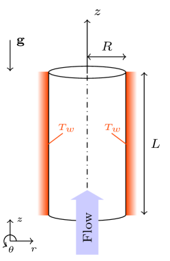
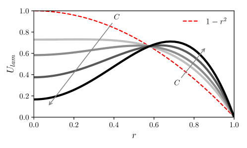
Figure 1: (Left) Schematic of the flow configuration A pipe section of length $L$ and radius $R$ is considered. The pipe is vertically aligned in the gravity field $\mathbf{g}$ and the fluid inside it is driven upwards by an externally applied pressure gradient and by buoyancy. The latter results from the lightening of the fluid close to the heated wall. We assume that the temperature at the wall $T_{w}$ remains constant in the pipe section. (Right) Laminar velocity profiles (11) for increasing values of $C$, as indicated by the arrows. Red dashed line: $C=0$ (isothermal profile). Light grey to black lines: $C=3$, 5, 7.5, 10.

The fluid has kinematic viscosity $\nu$, density $\rho$, volume expansion coefficient $\gamma$ and thermal diffusivity $\kappa$. Under the Boussinesq approximation, density variations are ignored except where they appear in terms multiplied by the acceleration due to gravity, $g\,\hat{\mbox{\boldmath$z$}}$, leading to the governing equations

$$\nabla\cdot\mbox{\boldmath$u$}=0\,,$$ (1)

$$\frac{\partial\mbox{\boldmath$u$}}{\partial t}+\mbox{\boldmath$u$}\cdot\mbox{\boldmath$\nabla$}\mbox{\boldmath$u$}=-\frac{1}{\rho}\mbox{\boldmath$\nabla$}p+\nu\,\nabla^{2}\mbox{\boldmath$u$}+\frac{1}{\rho}\,(1+\beta)\,\mathrm{d}_{z}P\,\hat{\mbox{\boldmath$z$}}+\gamma\,g\,(T-T_{ref})\,\hat{\mbox{\boldmath$z$}}\,,$$ (2)

$$\frac{\partial T}{\partial t}+\mbox{\boldmath$u$}\cdot\mbox{\boldmath$\nabla$}T=\kappa\,\nabla^{2}T-\epsilon\,,$$ (3)

where $T_{ref}$ is a reference temperature defined in the following subsection, and $\mathrm{d}_{z}P$ is the pressure gradient for laminar flow with bulk velocity $U_{b}$. We suppose that $U_{b}$ is fixed, in which case $\beta(\mbox{\boldmath$u$})$ adjusts to maintain fixed bulk velocity. We also suppose that the temperature of the wall $T_{w}$ and the bulk temperature $T_{b}$ are fixed. The latter is achieved by including a uniform heat sink $\epsilon(t)$ which adjusts to maintain the fixed bulk value $T_{b}$. For such a flow, we can introduce axial periodicity, so that $\epsilon(t)$ may be considered equivalent to the rate at which heat absorbed by the fluid would otherwise be carried out of the section of pipe.

For laminar flow, the flow is purely axial so that radial heat transport is purely conductive. If $\epsilon_{0}$ is the heating rate for the laminar case, then the observed quantity $\mbox{\it Nu}:=\bar{\epsilon}/\epsilon_{0}$ is the Nusselt Number, where the overbar $\overline{(\bullet)}$ denotes time average.

2.1 Non-dimensionalisation

Given the temperature at the wall $T_{w}$ and the bulk temperature $T_{b}$, we put $\Delta T=2(T_{w}-T_{b})$ and take a reference temperature $T_{ref}=T_{w}-\Delta\,T=2T_{b}-T_{w}=T_{c}$, where $T_{c}$ is the centreline temperature for the case of laminar flow. (The choice for $T_{ref}$ does not influence the flow, since the constant $\gamma\,g\,T_{ref}$ could be absorbed into the pressure gradient.) We introduce the dimensionless temperature $\Theta=(T-T_{c})/\Delta T$. Let the pipe radius $R=D/2$ be the length scale and the isothermal laminar centreline velocity $2\,U_{b}$ be the velocity scale. The corresponding time scale is thus $R/(2\,U_{b})$. Hereafter, all variables are dimensionless except $\epsilon(t)$ which always appears in the dimensionless ratio $\epsilon/\epsilon_{0}$, i.e. the instantaneous Nusselt number. Non-dimensionalising with these scales, for the temperature equation we find

$$\frac{\partial\Theta}{\partial t}+\mbox{\boldmath$u$}\cdot\nabla\Theta\,=\,\frac{\kappa}{2\,U_{b}R}\nabla^{2}\Theta-\frac{\epsilon R}{2\,U_{b}\,\Delta T}\,.$$ (4)

For the laminar case, $\Theta=\Theta_{lam}=r^{2}$, we find

$$0\,=\,\frac{\kappa}{2\,U_{b}R}\cdot 4-\frac{\epsilon_{0}R}{2\,U_{b}\,\Delta T}\quad\mbox{i.e.}\quad\Delta T\,=\,\frac{\epsilon_{0}\,R^{2}}{4\,\kappa}\,.$$ (5)

Plugging this $\Delta T$ back in to (4), we obtain the dimensionless temperature equation

$$\frac{\partial\Theta}{\partial t}+\mbox{\boldmath$u$}\cdot\nabla\Theta\,=\,\frac{1}{Re\,Pr}\nabla^{2}\Theta-\frac{4}{Re\,Pr}\,\frac{\epsilon}{\epsilon_{0}}\,,$$ (6)

where $Re:=U_{b}D/\nu$ is the Reynolds number and $Pr:=\nu/\kappa$ is the Prandtl number. For the momentum equation we find

$$\frac{\partial\mbox{\boldmath$u$}}{\partial t}+\mbox{\boldmath$u$}\cdot\nabla\mbox{\boldmath$u$}=-\nabla p+\frac{1}{Re}\nabla^{2}\mbox{\boldmath$u$}+\frac{4}{Re}\,(1+\beta)\,\hat{\mathbf{z}}+\frac{\gamma\,g\,\Delta T\,R}{(2\,U_{b})^{2}}\,\Theta\,\hat{\mathbf{z}}$$ (7)

The coefficient of the buoyancy term can be written

$$\frac{\gamma\,g\,\Delta T\,R}{4\,U_{b}^{2}}\,=\,\frac{1}{4}\,\frac{\gamma\,g\,(T_{w}-T_{b})\,D^{3}}{\nu^{2}}\,\frac{\nu^{2}}{U_{b}^{2}\,D^{2}}\,=\,\frac{1}{4}\,Gr\,Re^{-2}\,,$$ (8)

where $Gr:=\gamma\,g\,(T_{w}-T_{b})\,D^{3}/\nu^{2}$ is the Grashof number. Although the Grashof number is in common use, from $Gr$ it is difficult to judge the magnitude of the buoyancy force relative to the pressure gradient of the laminar flow for this particular configuration. We therefore write the dimensionless momentum equation as

$$\frac{\partial\mbox{\boldmath$u$}}{\partial t}+\mbox{\boldmath$u$}\cdot\nabla\mbox{\boldmath$u$}=-\nabla p+\frac{1}{Re}\nabla^{2}\mbox{\boldmath$u$}+\frac{4}{Re}(1+\beta+C\,\Theta)\,\hat{\mathbf{z}}\,,$$ (9)

where $C$ measures the buoyancy force relative to the force that drives the laminar isothermal shear flow,

$$C=\frac{Gr/(4\,Re^{2})}{4/Re}:=\frac{Gr}{16\,Re}.$$ (10)

The laminar velocity and laminar temperature profiles for this configuration are

$$U_{lam}(r)=\left(1-r^{2}\right)+C\left(\frac{1}{3}\,r^{2}-\frac{1}{4}\,r^{4}-\frac{1}{12}\right)\,,\qquad\Theta_{lam}(r)=r^{2}\,,$$ (11)

and the no-slip and fixed-temperature boundary conditions at $r=1$ are

$$\mbox{\boldmath$u$}=\mbox{\boldmath$0$},\qquad\Theta=1,$$ (12)

respectively, while periodic boundary conditions are applied in the streamwise direction. The laminar velocity profiles for different $C$ are shown in figure 1(right). The isothermal pipe flow is recovered for $C=0$ (no buoyancy force) and $Pr=0$ (temperature diffuses immediately), with the parabolic laminar profile $U_{0}=1-r^{2}$.

For a statistically steady flow, Reynolds averaging is both time averaging and cylindrical surface averaging, where the latter is denoted as

$$\langle(\bullet)\rangle(r):=\frac{1}{2\pi L}\int_{0}^{L}\int_{0}^{2\pi}(\bullet)\,\mathrm{d}\theta\,\mathrm{d}z\,.$$ (13)

Turbulent fluctuations are calculated as deviations from the mean components of the flow, i.e. $\left\{\mathbf{u}^{\prime}(\mathbf{x},t),\Theta^{\prime}(\mathbf{x},t)\right\}:=\left\{\mathbf{u}(\mathbf{x},t),\Theta(\mathbf{x},t)\right\}-\{\langle\overline{\mathbf{u}}\rangle(r),\langle\overline{\Theta}\rangle(r)\}$.

2.2 Numerics

Simulations were carried out using the Openpipeflow solver (Willis, 2017), modified to include timestepping of the temperature field and the buoyancy term in the momentum equation. A variable $q(r,\theta,z)$ is discretised using a non-uniform grid in the radial direction with points clustered near the wall and Fourier decompositions in the azimuthal and streamwise directions, namely

$$q(r,\theta,z)=\sum_{k<|K|}\sum_{m<|M|}q_{km}(r_{n})e^{i\alpha kz+m_{p}m\theta}\quad n=1,...,N$$ (14)

where $\alpha=2\pi/L$ is the streamwise wavenumber and $m_{p}$ determines the azimuthal periodicity ($m_{p}=1$ for no discrete rotational symmetry). Radial derivatives are evaluated using central finite differences with a nine-point stencil. At $Re=5300$, in a $L=5D$ long pipe we use a spatial resolution of $(N\times M\times K)=(64\times 96\times 96)$, which ensures a drop of at least 4 orders of magnitude in the spectra and provides the correct value for the friction factor, as reported in the literature (Eggels et al., 1994). Following the 3/2 dealiasing rule, variables are evaluated on an $N\times 3M\times 3K$ grid in physical space. A second-order predictor-corrector scheme is employed for temporal discretisation, and a fixed timestep of 0.01 is used. This is sufficient to ensure that the time discretisation error is no larger than the spatial discretisation error (measured by the corrector and spectra respectively) and corresponds to a CFL-number of approximately $0.2-0.25$.

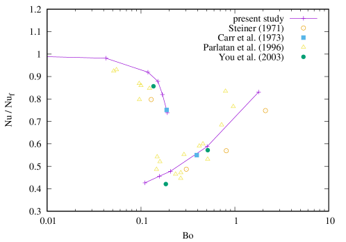
Figure 2: Change in $Nu$ flux, normalised by that for turbulent ‘forced convection’ ($C\to 0$), as a function of $Bo\,=\,8\times 10^{4}\,(8\,Nu\,Gr)\,/\,(Re^{3.425}Pr^{0.8})$. Data from simulations at $Re=5300$, $Pr=0.7$ and various $Gr=16\,Re\,C$. The upper and lower branches correspond to flow in shear-driven and convection-driven states respectively.

Data for simulations for various $Gr=16\,Re\,C$ and constant $Re=5300,\,Pr=0.7$ are shown in figure 2. There is good agreement with numerical data (You et al., 2003) and experimental data (Steiner, 1971; Carr et al., 1973; Parlatan et al., 1996).

2.3 Travelling wave solutions

In order to apply dynamical systems theory, the discretised momentum and temperature equations are formulated as an autonomous dynamical system (Viswanath, 2007; Willis et al., 2013):

$$\frac{\mathrm{d}\mathbf{X}}{\mathrm{d}t}=\mathbf{F}(\mathbf{X};\,\mathbf{p}),$$ (15)

where $\mathbf{X}$ is the vector of dependent variables, here $\mathbf{X}=(\mbox{\boldmath$u$},\Theta)$, and $\mathbf{p}$ is the vector of parameters of the system, $\mathbf{p}=(Re,C)$. The simplest solution is an equilibrium, which satisfies $\mathbf{F}(\mathbf{X};\,\mathbf{p})=0$. For pipe flow, the only equilibrium solution is the laminar solution. Travelling wave solutions satisfy $\mathbf{X}(\mbox{\boldmath$x$},t)=g(ct)\,\mathbf{X}(\mbox{\boldmath$x$},0)$, where here $g(l)$ applies a streamwise shift by $l$, and $c$ is the phase speed. Travelling waves are also known as ‘relative’ equilibrium solutions, as they are steady in a co-moving frame. They therefore satisfy

$$\mathbf{G}(\mathbf{X}(0),l,T)=g(-l)\mathbf{X}(T)-\mathbf{X}(0)=\mbox{\boldmath$0$}\,,$$ (16)

for some vector $(\mathbf{X},l,T)$, and hence can be calculated via a root solving method. The most popular method at present is the Newton–Krylov method. (Note that in addition to (16), two extra constraints are required to match the extra unknowns $l$, $T$; see Viswanath (2007).) Time-dependent periodic orbits may also be calculated by this method. Typically periodic orbits originate via a Hopf bifurcation off a travelling wave, but are not discussed further in this work.

Stability of the solutions is calculated using the Arnoldi method to solve the eigenvalue problem

$$\mathrm{e}^{\sigma T}\,\mathbf{dX}=g(-l)\,(\mathbf{X}_{0}+\mathbf{dX})(T)-\mathbf{X}_{0}(0)\,,$$ (17)

where $\sigma$ is the growth rate and the operator on the right hand side is linearised about the travelling wave $\mathbf{X}_{0}$ by taking $||\mathbf{dX}||\ll||\mathbf{X}_{0}||$. (Numerical performance is improved by replacing $\mathbf{X}_{0}(0)$ with $g(-l)\,\mathbf{X}_{0}(T)$ in (17).)

The Newton-Krylov and Arnoldi solver, already available as a utility of Openpipeflow (Willis, 2017), were integrated with the time-stepping code described in §2.2 for heated pipe flow.

3 Results and discussion

All results presented herein pertain to the case $Pr=0.7$ and constant volume flux. This relatively low Prandtl number is a reasonable starting choice for the applications we are interested in, where most gasses have $Pr\approx 0.7$, e.g. CO₂. In large scale cooling applications using liquid metal, $Pr$ is much smaller. Cases where $Pr>1$ (e.g. $Pr=7$ for water) are more expensive numerically due to a need for higher resolution for the temperature field.

3.1 Direct Numerical Simulations

Simulations were performed in a pipe of length $L=5D$ for a range of Reynolds numbers to study the effect of the buoyancy parameter $C$. Results are first shown for a relatively low Reynolds number, $Re=2500$. Figure 3 shows complete relaminarisation of transitional turbulence in response to the introduction of buoyancy for intermediate values of $C=\mathcal{O}(10^{-1})-\mathcal{O}(1)$. Relaminarisation events are revealed by monitoring the energy of the streamwise-dependent component of the flow, denoted $E_{3D}$, which shows a rapid decay when the flow relaminarises, $E_{3D}\to 0$ and $\varepsilon(t)/\varepsilon_{0}\to 1$. At larger $C\geq\mathcal{O}(10)$, turbulent fluctuations are not completely suppressed. Instead a convection-driven flow is set up, which becomes stronger as $C$ is increased.

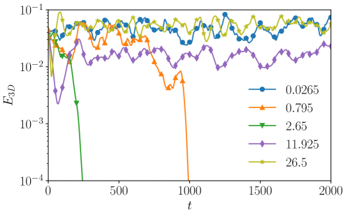
Figure 3: Energy of the streamwise-dependent component of the flow. $Re=2500$, $L=5D$, $Pr=0.7$ for a range of $C$ (values reported in the legend). Intermediate values of $C$ destabilise the turbulence, or even cause immediate relaminarisation.

At $Re=5300$ the effect of buoyancy is found to be slightly different – turbulence is not observed to undergo complete relaminarisation, but instead transitions directly to a weak convection-driven state. Figure 4 shows simulations with $C=O(1)-O(10)$. The buoyancy causes suppression of the turbulence and therefore a drop in $\varepsilon(t)/\varepsilon_{0}$, so that the Nusselt number $\mbox{\it Nu}=\bar{\varepsilon}/\varepsilon_{0}$ reduces substantially. The corresponding velocity and temperature mean profiles, $\langle u_{z}\rangle(r)$ and $\langle\Theta\rangle(r)$, are shown in bottom graphs of figure 4 together with the laminar profiles at $C=0$ for comparison. Cases where turbulence is suppressed exhibit a flattened base velocity profile.

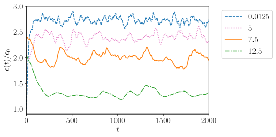
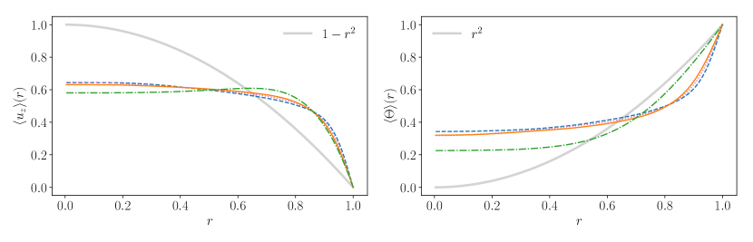
Figure 4: $Re=5300$, $L=5\,D$, $Pr=0.7$, resolution $64\times 96\times 96$. Top: Non-dimensional instantaneous heat flux, $\mbox{\it Nu}=\epsilon/\epsilon_{0}$ for different values of $C$, as indicated in the legend. Bottom: Snapshots of mean streamwise velocity $\langle u_{z}\rangle(r)$ and temperature $\langle\Theta\rangle(r)$ profiles at $t=1000$ for the same values of $C$ shown at the top. The thick light-grey lines correspond to the laminar profiles (11) with $C=0$.

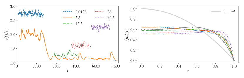
Figure 5: Parameters as in figure 4 but for larger $C$ (values reported in the legend). Left: Non-dimensional instantaneous heat flux, $\mbox{\it Nu}=\epsilon/\epsilon_{0}$. The initial transients ($t\approx 100-200$) are omitted for all trajectories and the curves corresponding to $C\geq 12.5$ are shifted in time by an arbitrary offset, for clarity only. Right: Snapshots of the mean streamwise velocity profiles $\langle u_{z}\rangle(r)$ for the same values of $C$ shown on the left. All the snapshots are taken at $t=1000$. For $C=7.5$ an additional snapshot (solid grey line with dots) is shown corresponding to $t=7500$ (marked with a grey dot on the corresponding trajectory on the left). The thick light-grey line on the right corresponds to the laminar streamwise velocity profile (11) with $C=0$.

The case for $C=7.5$ is shown for longer time in figure 5(left). The shear-driven turbulent state is metastable only, and around $t\approx 2000$ turbulence is more suppressed as there is a switch to the more quiescent convection-driven state. As $C$ is increased further the buoyancy starts to drive a more turbulent convection-driven state. For these cases the velocity profile is more ‘M-shaped’ as seen in figure 5(right).

The convective state at $Re=5300$ and $C=7.5$ is visualised in figure 6 together with the metastable shear-driven turbulent state. When comparing the deviations from the isothermal laminar profile (a–d), both the shear and convective states show a deceleration in the core and acceleration close to the wall, with the convective states showing very smooth and almost $z-$ and $\theta-$independent contour levels. Deviations from the mean profile (e–h), however, reveal that the convective state has larger and more elongated flow structures compared to the shear-driven turbulence. In both types of visualisations it is clear that the small-scale turbulent eddies are strongly suppressed in the convection-driven flow.

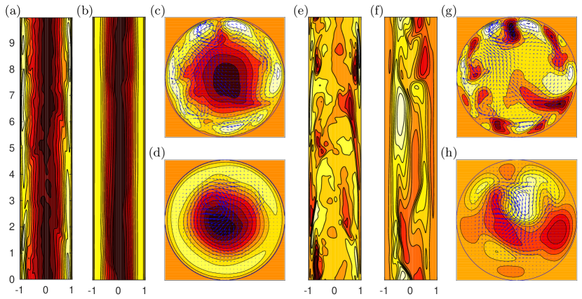
Figure 6: Isolevels of streamwise velocity perturbation for (a, c, e, g) the shear-driven turbulence and (b, d, f, h) the convective state at $Re=5300$, $C=7.5$ and $t=1000$, $t=7500$, respectively. (The corresponding streamwise velocity profiles at these times were shown in 5(right).) Plots on the left (a–d) show deviations from the isothermal laminar profile $U_{0}=1-r^{2}$, while plots on the right (e–h) show deviations from the mean profile $\langle u_{z}\rangle(r)$. Dark/light regions correspond to slow/fast streaks. Ten contours are used between the maximum and minimum values, corresponding to (a–d) $u-U_{0}\in[-0.4,0.3]$, (e, g) $u^{\prime}\in[-0.2,0.1]$ and (f, h) $u^{\prime}\in[-0.1,0.08]$. The arrows in the $r-\theta$ cross-sections (c, d, g, h) indicate the cross-sectional velocity components, multiplied by a factor of 2 for the shear turbulence (c, g) and 5 for the convective state (d, h), for visualisation reasons only. The $r-\theta$ cross-sections (c, d, g, h) are taken at $z=0$ while the $r-z$ sections are taken at $\theta=\pi/2$.

Figure 7 shows the type of state seen in simulations, laminar flow (L), shear-driven turbulence (S) and convection-driven flow (C), for a range of $Re$ and $C$. The initial condition for each simulation was a previously calculated shear-driven state at similar $Re$. (This is except for $Re\leq 2000$ and $C>3$, where it is clear that the shear-driven state decays immediately, i.e. only the convective state could be supported, and hence the initial condition was of convection type). For each simulation it is relatively easy to distinguish between the shear- and convection-type flows, since the former shows far more chaotic time series and higher heat flux. The case for $C=7.5$ in figure 5(left) shows this difference, and also that multiple behaviours are possible at the same parameters for significant periods of time. The shear-driven state is marked if observed for $\gtrsim 1000$ time units. (It is stable or at least metastable with a long expected lifetime.) A relaminarisation is marked if the energy of the streamwise component of the flow drops below $10^{-5}$. Overall, figure 7 indicates that as $C$ (or $Gr$) increases, a larger $Re$ is needed in order to drive shear turbulence, or, equivalently, as $Re$ increases, shear-driven states persist to larger $C$. For $C\geq 4$ simulations suggest that a convective instability kicks in, roughly independently of the Reynolds number over this range. In between, it is possible to completely relaminarise flow up to $Re\approx 3500$, but at larger $Re$ the progression is as in figure 5 – from a shear-driven turbulent state to a weak convection-driven state, then to a more turbulent convection-driven state as $C$ is increased.

In the following sections we determine whether the boundaries of stability observed in figure 7 are consistent with linear stability of the laminar flow, analysis of travelling wave solutions and the viewpoint of HHS.

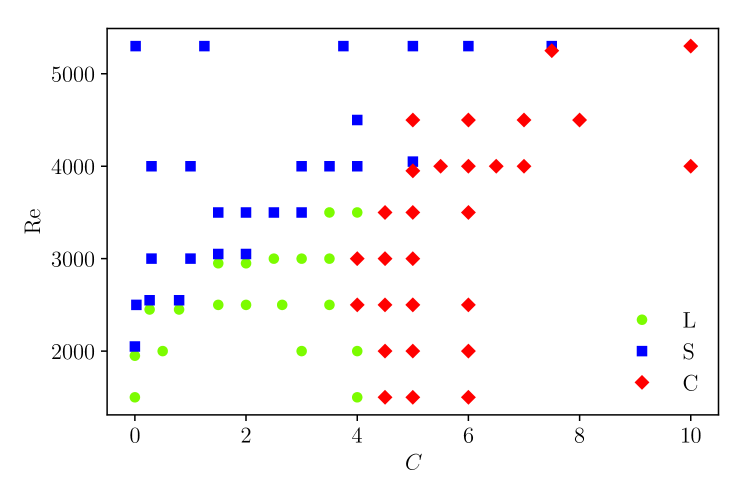
Figure 7: Regions of laminar (L) flow, shear-driven (S) turbulence and convection-driven (C) flow. Points where multiple behaviours are observed are marked with a slight offset in $Re$. Simulations are initiated with a previously calculated shear-driven state at similar $Re$, except for the region $Re\leq 2000$ and $C>3$ where the shear-driven state decays immediately and hence simulations are started with a convection-driven state.

3.2 Linear stability analysis

As the transition to shear-driven turbulence in isothermal flow occurs in the absence of a linear instability, this section relates to the transition to convection-driven flow states, in particular with respect to loss of stability of the modified laminar base profile (11) for non-zero $C$. Linear stability of mixed-convection pipe flow has been studied by Yao (1987a); Su & Chung (2000), where the model differs slightly in the boundary condition and form of the heat sink. Our figure 2 suggests these differences make little difference to transition, however, we check for consistency with the nonlinear results of §3.1.

As our code uses Fourier expansions in the periodic dimensions, to calculate the eigenfunctions and stability of the base flow (11) we need simulate only using a few Fourier modes. The Arnoldi method is employed to accelerate convergence and to access eigenvalues beyond the leading one. Linear stability analysis is performed for azimuthal wavenumbers $m=0,1,2$ and two streamwise wavenumbers $\alpha=0.628$ and $\alpha=1.7$ (commensurate with the pipe lengths $L=5D$ and $L=1.85D$ used in our DNS study of §3.1 and in the travelling wave analysis of §3.3).

The neutral curves, where the growth rate $\Re(\sigma)=0$, are shown in figure 8. As expected (and as also reported by Yao (1987a); Su & Chung (2000)), the first azimuthal mode is found to be the least stable, it corresponds to the spatially largest mode and is the only mode that can exhibit flow across the axis. (The axisymmetric mode $m=0$ is included in the numerical calculations for stability of the $m=1$ mode, but we have not observed instability of $m=0$ type.) As shown in figure 8, the $m=1$ mode exhibits a fairly complex dependence on $C$, while it is only weakly affected by the axial wavenumber. Indeed, the first branch for $\alpha=0.628$ almost coincides with that for $\alpha=1.7$ and the other two branches (not shown) are slightly shifted to the right. Consistent with the linear stability of isothermal pipe flow, the critical Reynolds number approaches infinity as $C\to 0$ for any $m$.

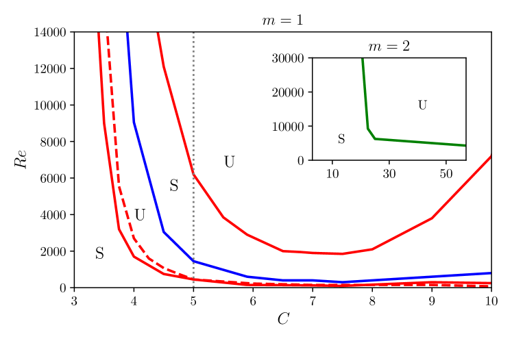
Figure 8: Linear stability analysis for $\alpha=1.7$, $k=1$ ($L=1.85D$) (solid lines). Main figure: $m=1$. Inset: $m=2$. The axisymmetric mode is included in the $m=1$ analysis (i.e. $m=0$ and $\pm 1$), but instability of this mode is not observed. The first branch (for $m=1$) is also shown for the case $\alpha=0.628$ (dashed line). The neutral curves delimit regions where the flow is linearly stable (S) or unstable (U). The dotted vertical line indicates the value of $C$ ($C=5$) at which the growth rate is shown in figure 9 as a function of $Re$.

Consistent with the appearance of the convective state found in simulation (figure 7), at $C\approx 4$ a linear instability appears, roughly independent of $Re$ for most of the range considered. The corresponding laminar profiles for $C=3-10$ are shown in figure 1(right). For $C>4$ the profiles present an “M-shape” (independent of $Re$, see (11)), which becomes increasingly more pronounced as $C$ increases. The difference at the centreline is more than 80% for $C=10$. The profile at $C=3$ is flatter than the parabolic (isothermal) profile, with a centreline difference of almost 30%, but does not have any inflection point. Therefore, in agreement with previous experimental and theoretical studies (Scheele & Hanratty, 1962; Yao, 1987a; Su & Chung, 2000), our analysis suggests that the linear instability of buoyancy-assisted pipe flow is linked to the inflectional velocity profiles ocurring at sufficiently large heating and it is almost independent of $Re$.

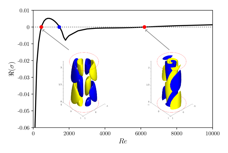
Figure 9: Growth rate vs Reynolds number from linear stability analysis at $\alpha=1.7$, $k=1$ ($L=1.85D$), $m=1$ and $C=5$ (corresponding to the dotted vertical line in figure 8). Insets: streamwise vorticity (blue/yellow are 30% of the min/max value) close to the two neutral points ($Re\approx 400$ and 6200).

Figure 8 also shows that, for $C\gtrsim 4$, a region of restabilisation is observed as $Re$ is increased. This is also evidenced in figure 9, which shows a region of negative $\Re(\sigma)$ for $1450<Re<6200$ at $C=5$. Isosurfaces of streamwise vorticity for the eigenfunctions corresponding to the two neutral points where $\Re(\sigma)$ becomes positive ($Re\approx 400$ and 6200) are also shown in the insets of figure 9. For the larger Reynolds number, $Re\approx 6200$, the eigenfunction looks like it is spiralling in the centre and resembles the “spiral” solution found by Senoo et al. (2012), although their visualised solutions are nonlinear.

3.3 Continuation from $\mathrm{TW_{N4L}}$

To better understand the effect of buoyancy, we perform a nonlinear analysis, starting from a known TW in isothermal pipe flow ($C=Gr=0$) and continuing the solution to larger values. A vast repertoire of TWs has now been compiled in isothermal pipe flows (Budanur et al., 2017). For our purpose we decided to focus on a fundamental solution, labelled $\text{TW}_{\text{N4L}}$ (Pringle et al., 2009), which is highly-symmetric (satisfying both shift-reflect and shift-rotate symmetries) and characterised by relatively smooth continuation branches in order to aid the numerical continuation. In Willis et al. (2013), the lower branch of this solution was found to lie on the boundary between the laminar state and turbulence in a ‘minimal flow unit’. Localised solutions bifurcate off this class of solutions (Chantry et al., 2014) and are found to mediate transition in extended domains (Avila et al., 2013; Budanur & Hof, 2017).

Following Willis et al. (2016) we start with the ‘minimal flow unit’ at Reynolds number $Re=2500$ with domain $(r,\theta,z)=[0,\,1]\times[0,\,\pi/2]\times[0,2\pi/1.7]$, i.e. $m_{p}=4$ and $\alpha=1.7$ in (14). For isothermal flow ($C=Gr=0$), the phase speed of $\text{TW}_{\text{N4L}}$ is $c=0.61925$. The isothermal TW was first reconverged at $Pr=0.7$ using the Newton solver. A parametric continuation in $C$ to non-zero values was then performed (figure 10) for fixed $Re$, $Pr$ and $\alpha$. We were able to continue the isothermal solution from $C=0$ around positive $C$ and find that it connects with the upper branch at $C=0$, then beyond to $C\approx-40$. (Negative $C$ corresponds to a downward cooled flow; see Appendix A). As a check, we verified that the values of $c=0.52575$ and $Nu=2.378$ at $C=0$ on the upper branch, as well as the mean profiles, matched those of the previously known upper-branch isothermal solution $\text{TW}_{\text{N4U}}$ with $Pr=0.7$.

In figure 10(right) it is seen that from $C=0$ to $C=6$ the Nusselt number Nu increases by approx 0.75. By comparison, along the upper branch, over the large range $C=6$ to $C=-40$, it increases by only a further 1.25. Relatively speaking, the lower branch is rapidly pushed back towards the upper branch over the increase in $C$ and is suppressed altogether for $C>7.5$.

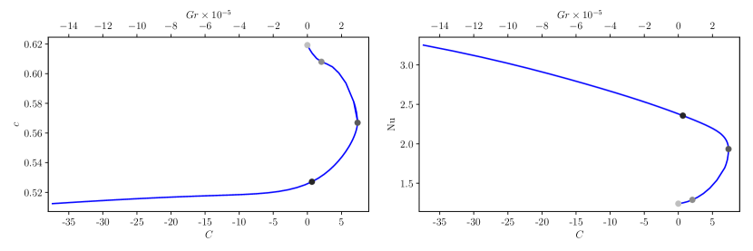
Figure 10: Continuation in $C$ (or $Gr$) from N4L at $Re=2500$. (a) Phase speed $c$ vs $C$ (or $Gr$), (b) Nu vs $C$ (or $Gr$). Filled circles indicate the points along the continuation at which the mean streamwise velocity and temperature profiles are shown in figure 11.

The mean velocity and temperature profiles at different points along the continuation are shown in figure 11. Observe that the profile in the near-wall region, where rolls and streaks occur, is similar at the saddle-node point (SN) to that of the isothermal upper branch (UB) solution.

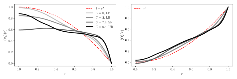
Figure 11: Mean streamwise velocity (left) and temperature (right) profiles at the points along the continuation from N4L ($Re=2500$) marked in figure 10 (SN: saddle node, LB/UB: lower/upper branch). The temperature profiles for $C=0$ and $C=2$ on the lower branch are indistinguishable.

Figure 12(left) shows these rolls (arrows) and streaks (contours) in cross sections of the velocity perturbation at the saddle-node point. The corresponding temperature perturbation field (‘thermal streaks’) is shown on the right. Similar to its isothermal counterpart, the travelling wave is characterised by fast streaks located near the pipe wall and slow streaks in the interior. The core shows a strongly decelerated region relative to the laminar (isothermal) profile and thus the profile must become steeper at the wall to preserve the mass-flux. The difference from the isothermal $\mathrm{TW_{N4L}}$, however, is less marked in the near-wall region than it is in the core.

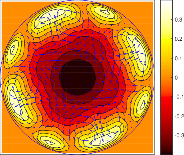
(a)

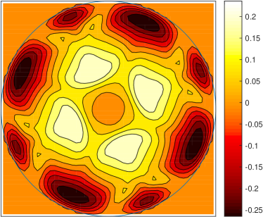
(b)

Figure 12: Cross sections of streamwise velocity (left) and temperature (right) perturbations (deviations from the isothermal laminar flow) for the N4L travelling wave at $Re=2500$ and $C=7.4$ (saddle node). Ten contours are used between the maximum and minimum. The arrows in the left graph indicate the cross-sectional velocities

Continuations were also performed at $Re=2000$ and $3000$, after reconverging the isothermal $\text{TW}_{\text{N4L}}$ at these Reynolds numbers. Results are shown in figure 13.

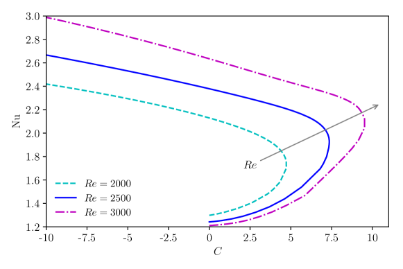
Figure 13: Continuation in $C$ from N4L for increasing values of $Re$. The curve for $Re=2500$ is the same as that shown in figure 10(right).

The TW survives to larger $C$ as the Reynolds number increases (the saddle-node point of each curve moves to larger $C$ as $Re$ increases). This is consistent with the shear turbulence region in figure 7 persisting to larger $C$ as $Re$ is increased. The saddle-node bifurcations at each $Re$ occur at much larger values of $C$ than those at which suppression of turbulence was observed in the DNS. For example, at $Re=2500$ the saddle-node bifurcation occurs at $C\approx 7.5$, while in figure 7 shear-turbulence survives only for $C\lesssim 1$. This is not so surprising, considering that in isothermal pipe flows the lowest $Re$ at which the N4L travelling-wave solution is found, i.e. $Re=1290$ (Pringle et al., 2009), is much below the commonly observed value for transition in experiments ($Re\approx 1800-2300$). Furthermore, it should be taken into account that only one TW solution is analysed here – it cannot capture the entire phenomenon of turbulence suppression in a heated pipe flow, although is found to capture some of the fundamental characteristics.

Figure 14 shows that, while the lower branch solution for $Re=3000$ is on the edge of an attractor for shear-driven turbulence at $C=0$, this is no longer the case for $C=4$. Shear-driven turbulence does not survive in the heated case, although shooting in the upper direction for $C=4$ does still produce a short turbulent transient. In particular, large amplification of the initial disturbance still occurs in the heated case, but the self-sustaining mechanism appears to be disrupted.

To summarise this section, we have observed that a known TW solution of the isothermal pipe flow is suppressed by buoyancy and that it is connected to the transition to turbulence. The observations are consistent with destabilisation of the shear-driven turbulent state, but at this stage another approach is required to forge an approximate quantitative link with the transition from turbulence.

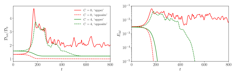
Figure 14: Times series of (left) total dissipation $\mathcal{D}_{tot}$ (normalised by the laminar isothermal value $\mathcal{D}_{0}=2\pi L_{z}|-2|=4\pi L_{z}$) and (right) energy of the streamwise-dependent modes $E_{3d}$ for simulations started from the lower-branch TW solutions at $Re=3000$, $\alpha=1.7$ with $C=0$ and $C=4$. The TW is perturbed by adding $\mp\,0.001\,(\mathbf{w}_{1}+0.01\mathbf{w}_{2})$ (denoted as ‘upper’ and ‘opposite’ directions) where $\mathbf{w_{1}}$ and $\mathbf{w_{2}}$ are the first (leading) and second eigenvectors. Shooting in the ‘upper’ direction leads to turbulence for $C=0$, while the flow goes back to laminar when perturbed in the opposite direction. For $C=4$ both directions end up at the laminar point.

3.4 Calculation of the apparent Reynolds number of HHS

In §1.2, where we gave a brief overview of HHS, the (isothermal) equivalent pressure gradient flow (EPG flow) was identified as a useful reference case for heated flows. To calculate the apparent Reynolds number of the EPG reference flow, one must determine the contribution to the mass flux from the buoyancy force that would have been induced in a fixed pressure-gradient flow. Here we summarise the key points of the analysis of HHS and apply it to a selected example case from our data. (The interested reader is referred to sections 3.3 and 3.5 of HHS for a detailed derivation.) In the following section we relate HHS analysis to the phase diagram determined from the simulations of §3.1.

The analysis starts by decomposing the body-force influenced flow (i.e. the total flow) into a pressure-driven flow of equivalent pressure gradient (the EPG reference flow) and a perturbation flow due to the body force,

$$\mathbf{u}(\mathbf{x},t)=\mathbf{u}^{\dagger}(\mathbf{x},t)+\mathbf{u}^{f}(\mathbf{x},t)$$ (18)

where the superscripts ${\dagger}$ and $f$ denote the EPG and the body-force perturbation driven flows, respectively. In contrast to the conventional view, HHS observe that adding a non-uniform (radially-dependent) streamwise body force to a flow initially driven only by a pressure gradient does not alter its turbulent mixing characteristics and in particular the turbulent viscosity remains approximately the same. From this point of view, the body-force influenced flow behaves in the same way as the EPG flow and relaminarisation occurs when the Reynolds number $Re_{app}$ of this ‘apparent’ flow drops below a certain threshold where turbulence cannot be sustained any more. Given the difficulties discussed in §1 to uniquely define a critical Reynolds number for transition, we decided to follow HHS and select a nominal value of 2300, as quoted in many engineering textbooks (see e.g. White, 1979). By writing the bulk velocity $U_{b}$ of the EPG flow as the difference between that of the total flow and of the body-force perturbation driven flow, i.e. $U_{b}^{\dagger}=0.5-U_{b}^{f}$, the above relaminarisation criterion can be expressed as

$$Re_{app}:=Re\,\left(1-2\,U_{b}^{f}\right)<2300\,.$$ (19)

To determine $U_{b}^{f}$, the following expression was derived by integrating three times the Reynolds-averaged $z$-momentum equation of the body-forced perturbation flow:

$$U_{b}^{f}:=Re\left[\underbrace{\frac{1}{2}\int_{0}^{1}(1-r^{2})f(r)\,r\mathrm{d}r}_{\mathcal{I}_{1}}+\underbrace{\int_{0}^{1}r\mathscr{R}_{uv}^{f}(r)\,r\mathrm{d}r}_{\mathcal{I}_{2}}\right]$$ (20)

where $\mathscr{R}_{uv}^{f}(r):=\langle\overline{(u_{z}^{\prime}u_{r}^{\prime})^{f}}\rangle$ is the Reynolds shear stress due to the perturbation flow induced by the body force $f(r)$. The first integral of (20), $\mathcal{I}_{1}:=\frac{1}{2}\int_{0}^{1}(1-r^{2})f(r)\,r\mathrm{d}r$, represents the direct contribution of the body force (which is assisting the flow), while the second integral, $\mathcal{I}_{2}:=\int_{0}^{1}r\mathscr{R}_{uv}^{f}(r)\,r\mathrm{d}r$, corresponds to the turbulent contribution related to the body-force perturbed flow. The Reynolds stress term $\mathscr{R}_{uv}^{f}$ of the body-force perturbed flow is related to that of the total ($\mathscr{R}_{uv}$) and EPG ($\mathscr{R}_{uv}^{\dagger}$) flows by using the decomposition (18) and is approximated by introducing the eddy viscosity concept,

$$\mathscr{R}_{uv}^{f}(r)=\mathscr{R}_{uv}(r)-\mathscr{R}_{uv}^{\dagger}(r)=\frac{\nu_{t}}{Re}\frac{\mathrm{d}\mathscr{U}_{z}}{\mathrm{d}r}-\frac{\nu_{t}^{\dagger}}{Re}\frac{\mathrm{d}\mathscr{U}_{z}^{\dagger}}{\mathrm{d}r}\,,$$ (21)

where $\mathscr{U}_{z}(r):=\langle\overline{({u}_{z})}\rangle$, $\mathscr{U}_{z}^{\dagger}(r):=\langle\overline{({u}_{z})^{\dagger}}\rangle$ and $\nu_{t}$ and $\nu_{t}^{\dagger}$ are the eddy viscosities of the total and EPG flows, respectively. Under the assumption that $\nu_{t}=\nu_{t}^{\dagger}$, we obtain

$$\mathscr{R}_{uv}^{f}(r)=-\frac{\nu_{t}^{\dagger}}{Re}\frac{\mathrm{d}\mathscr{U}_{z}^{f}}{\mathrm{d}r}\,,$$ (22)

where the perturbation flow $\mathscr{U}_{z}^{f}(r):=\langle\overline{({u}_{z})^{f}}\rangle$ due to the imposed body force is obtained by integrating the Reynolds-averaged $z$-momentum equation

$$0=\frac{1}{r}\frac{\mathrm{d}}{\mathrm{d}r}\left[\frac{r}{Re}\left((1+\nu_{t}^{\dagger})\frac{\mathrm{d}\mathscr{U}_{z}^{f}}{\mathrm{d}r}\right)\right]+f\,,$$ (23)

provided that the EPG flow (and hence $\nu_{t}^{\dagger}$) is known. Equations (22) and (23) correspond to equations (3.6) and (3.7) of HHS and the reader is referred their sections 3.3 and 3.5 for a detailed derivation.

Here, we apply the criterion for relaminarisation (19) proposed by HHS to our model for a vertical heated pipe. The radially dependent body-force is $f_{0}=(4C/Re)\langle\overline{\Theta}\rangle(r)$. Since the body-force in HHS is zero at the axis, we shift the temperature profile by its value at the axis $\left.\langle\overline{\Theta}\rangle\right|_{r=0}$ and absorb this constant into the pressure gradient (see figure 15). This leads to the body force

$$f_{1}(r)=(4C/Re)\Big{[}\langle\overline{\Theta}\rangle-\left.\langle\overline{\Theta}\rangle\right|_{r=0}\Big{]}$$ (24)

and a fixed-pressure Reynolds number

$$Re_{p}=Re\Big{[}(1+\beta)+C\left.\langle\overline{\Theta}\rangle\right|_{r=0}\Big{]}$$

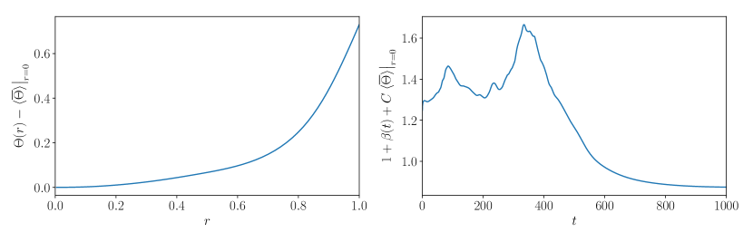
Figure 15: Application of HHS’s relaminarisation criterion (20) in the case $C=2$ and $Re=3000$. Left: Temperature profile shifted by $\left.\langle\overline{\Theta}\rangle\right|_{r=0}$. Right: the corresponding pressure gradient.

Initially, we consider the simulation with $C=2$ and $Re=3000$ for which it is observed that $Re_{p}=4252.71$. By inserting $f=f_{1}$ in $\mathcal{I}_{1}$ we obtain $Re\,\mathcal{I}_{1}=0.12$. To calculate $\mathcal{I}_{2}$ we need to evaluate the EPG flow in order to obtain $\nu_{t}^{\dagger}(r)$ and hence the Reynolds stress term $\mathscr{R}_{uv}^{f}(r)$ via (22) and (23). By definition, $Re_{p}^{\dagger}=Re_{p}$. In an approach similar to Willis et al. (2010), summarised in Appendix B, the eddy viscosity $\nu_{t}^{\dagger}(r)$ of the EPG reference flow is calculated using an expression originally suggested by Cess (1958), see (35). The resulting eddy viscosity is shown in figure 16(left).

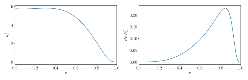
Figure 16: Eddy viscosity (left) of the EPG flow and Reynolds shear stress (right) of the body-force perturbed flow in the case $C=2$ and $Re=3000$. The eddy viscosity is calculated following an approach similar to Willis et al. (2010), as summarised in Appendix B. Once $\nu_{t}^{\dagger}$ is known, $\mathscr{R}_{uv}^{f}(r)$ is calculated using (22), together with (23).

By substituting $\nu_{t}^{\dagger}$ in (23) we can invert for $\mathrm{d}\mathscr{U}_{z}^{f}/\mathrm{d}r$ which plugged into (22) gives us the Reynolds stress $\mathscr{R}_{uv}^{f}(r)$ (see figure 16(right)). Finally, by inserting the latter in the second integral of (20) we obtain $Re\,\mathcal{I}_{2}=0.0405$. Putting everything together, (20) gives $U_{b}^{f}=Re\mathcal{I}_{1}+Re\mathcal{I}_{2}=0.12+0.0405\approx 0.16$. Then, using (19), $Re_{app}=Re\,\left(1-2\,U_{b}^{f}\right)=2040<2300$, i.e. the flow is expected to relaminarise. This value obtained for the apparent Reynolds number is reasonable, since relaminarisation occurs after approximately 400 time units (see figure 15 (right)).

3.5 HHS prediction of phase diagram and nonlinear dynamics

We now consider the general case of a flow at $Re$ with heating $C$, while introducing a number of approximations to simplify the analysis.

Firstly, the case discussed in §3.4 ($C=2$ and $Re=3000$) suggests that $Re\,\mathcal{I}_{1}$ has a significantly greater contribution than $Re\,\mathcal{I}_{2}$ in determining the body-force perturbation flow. This is found to be generally true for the cases considered herein, as well as those discussed in HHS, and hence we omit the term $Re\,\mathcal{I}_{2}$ for simplicity below. The perturbation flow due to the body force can thus be evaluated as

$$U_{b}^{f}\approx Re\,\mathcal{I}_{1}=\frac{1}{2}Re\int_{0}^{1}(1-r^{2})f(r)\,r\mathrm{d}r=2C\int_{0}^{1}(1-r^{2})\Big{[}\langle\overline{\Theta}\rangle-\left.\langle\overline{\Theta}\rangle\right|_{r=0}\Big{]}\mathrm{d}r\,,$$ (25)

where (24) has been used for $f(r)$.

Secondly, figure 4(bottom right) shows that the temperature mean profiles are remarkably similar in all turbulent shear-driven flows (i.e. ignoring the laminar or convection driven flow states), as far as the integral part of the right-hand side of (25) is concerned, despite that the values of the Nu (proportional to the gradient at the wall) are necessarily quite different for different cases. For the case $Re=5300$ $C=3.75$, for the left-hand side of (25) we obtain $Re\,\mathcal{I}_{1}=0.164$. By applying the above assumption,

$$U_{b}^{f}\approx Re\,\mathcal{I}_{1}=\frac{0.164}{3.75}\,C=0.04\,C$$ (26)

Let $Re_{app}$=2300 to find the critical $C$ for flow laminarisation, that is,

$$Re(1-2U_{b}^{f})=Re(1-0.08\,C)=2300$$ (27)

or

$$C_{cr,1}=12.5\left(1-\frac{2300}{Re}\right)\,.$$ (28)

For $C\gtrsim C_{cr,1}$ we expect to see rapid transition from the shear-driven turbulent state to the convective state. Noting $C=Gr/(16Re)$, the above can be expressed as a critical Grashof number:

$$Gr_{cr,1}=200(Re-2300)$$ (29)

Let us now consider the opposite scenario in which the flow under heating $C$ is either laminar or convection driven. Figure 4(bottom right) shows that the temperature profiles in such flows are significantly different from those in a turbulent shear-driven flow, and generally with a much thicker thermal boundary layer, and hence a greater buoyancy force. Consider the extreme case when the radial heat transfer is purely due to conduction and the temperature distribution is given by $\langle\overline{\Theta}\rangle=r^{2}$. The buoyancy-driven perturbation flow is therefore

$$U_{b}^{f}\approx Re\,\mathcal{I}_{1}=2C\int_{0}^{1}(1-r^{2})\,r^{2}\,\mathrm{d}r=\frac{C}{6}$$ (30)

Then a second critical $C=C_{cr,2}$ can be evaluated,

$$C_{cr,2}=6\left(1-\frac{2300}{Re}\right)\,,$$ (31)

below which the flow is expected to transition to the shear-driven turbulent flow. To put it another way, it is predicted that metastability of the shear-driven turbulent state should not be observed for $C\lesssim C_{cr,2}$, so that the turbulent state is stable. Between $C_{cr,1}$ and $C_{cr,2}$ the shear-driven state is expected to be metastable, so that this or a convective state may be observed. In terms of the Grashof number,

$$Gr_{cr,2}=96(Re-2300).$$ (32)

Equations (28) and (31) are plotted on the $Re-C$ graph in figure 17 together with all DNS results already presented in figure 7. The data of figure 7 was obtained starting from shear-driven turbulent states. Some additional simulations were performed at $Re=5300$ starting from convection-driven states and are reported in figure 17 using hollow symbols, with a slight offset in $Re$ for visualisation reasons. Note that in a $Re-Gr$ graph (29) and (32) are straight lines (see the inset in figure 17).

Considering a series of DNS runs for a fixed $Re$, for example $Re=5300$, but increasing $C$ values (heating) starting from $C=0$, equation (28) gives the critical $C=C_{cr,1}$ above which the flow will be laminarised or switch to convection-driven. On the other hand, starting from a large $C$ when the flow is laminarised or convective, equation (31) predicts a critical $C=C_{cr,2}$ below which the flow will be turbulent when sufficient disturbances are provided in the DNS. As $C_{cr,1}$ is larger than $C_{cr,2}$ for a given $Re$, there is an overlap in the possible state of flow, and consequently there is a hysteresis region in which the flow may or may not be laminarised, depending on the initial flow of the simulation (or experiment). As a result, the $Re-C$ plane can be divided into three regimes by the curves representing the two equations, i.e., turbulent shear-driven flow (regime I), convection-driven or laminar flow (regime III) and regime II in which either of the above may happen dependent on the initial flow. Note that for the Reynolds number range considered here, the linear stability curve (showed as a dashed grey line in figure 7) is always to the right of $C_{cr,2}$, i.e. $C_{cr,2}<C_{LS}$ . The two curves cross at $Re\approx 6000$ (not shown), which means that, for $Re<6000$ the convective flow is always linearly stable if $C<C_{cr,2}$. Hence, below $Re\approx 6000$, shear driven turbulence may be observed for $C<C_{LS}$.

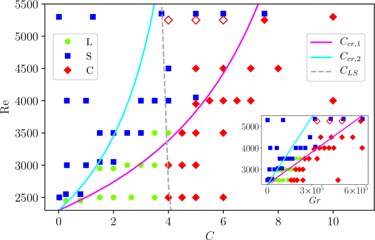
Figure 17: Regions of laminar (L) flow, shear-driven (S) turbulence and convection-driven (C) flow, as in 7, together with equations (28) and (31) and the linear stability stability curve (dashed red curve in figure 8). Initial conditions are a shear-driven turbulent state, except for the hollow symbols at $Re=5300$ which are started with a convection driven state, and similarly cases towards the bottom-right, where it is clear that the shear-driven state decays immediately.

A plot showing the phase transitions for the fixed Reynolds number $Re=5300$ is provided in figure 18, where the Nusselt number is displayed as a function of $C$ for simulations started with either shear-driven or convection-driven states. The two critical $C$ at this Reynolds number, $C_{cr,1}=7.1$ and $C_{cr,2}=3.4$, are indicated with vertical lines in figure 18. Starting from an unheated ($C=0$) turbulent flow, applying a low heating ($C\lessapprox 7$), we observe that the flow remains turbulent over the entire period of simulation ($t=2000$). The dynamics thus sits on the upper branch shown in figure 18. As $C$ is increased, the lifetime of shear-turbulence drops below 2000 time units for $C\gtrapprox 7.5$ and turbulence only survives for less than 500 time units at $C=10$. It then switches to the convection-type flow. This behaviour is marked in figure 18 by plotting the upper-branch curve with a dashed line for $C\geq 7.5$ until it crosses the lower-branch at $C=12.5$. At this value of $C$, indeed, the switch to the convective flow appears to be immediate. Now, starting from this convection-driven flow and applying a lower $C$, the flow remains convection-driven turbulent for $C\geq 3.8$, or relaminarises for $C\lessapprox 3.8$. This value of $C$ corresponds to the onset of the linear instability, which is responsible for the kink in Nu as $C$ is decreased. Our previous analysis predicts that for flows on the left of (31), their $Re_{app}$ is greater than 2300, hence they may be prone to transition to turbulence subject to sufficient disturbances. Correspondingly, the lower-branch curve in figure 18 is plotted with a dashed line for $C<C_{cr,2}=3.4$ to indicate that in practice (e.g. in a lab experiment) the flow would become shear-driven turbulent again. However, as previously discussed, at this Reynolds number, $C_{cr,2}<C_{LS}$. Bistability (between shear or convection driven states) is thus observed for $3.8\lessapprox C\lessapprox 7.5$. The latter value is in very good agreement with the threshold $C_{cr,1}=7.1$ predicted above.

In figures 19 and 20 the turbulent structures of the isothermal and heated flows at $Re=5300$, $C=0$ and $5$, are compared to those of the EPG reference flow. The latter was computed by performing a DNS with fixed pressure gradient such that $Re_{p}^{\dagger}=Re_{p}=10898.7$. The flow structures - streaks and vortices - are visualised as isosurfaces of streamwise velocity and streamwise vorticity fluctuations, normalised by the apparent friction velocity based on the pressure gradient component of the wall shear stress only, $u_{\tau p}^{*}$, where the asterisk ^∗ denotes a dimensional quantity here. The resulting apparent friction Reynolds number is $Re_{\tau p}:=u_{\tau p}^{*}R^{*}/\nu^{*}=Re_{\tau}^{\dagger}=147.6$.

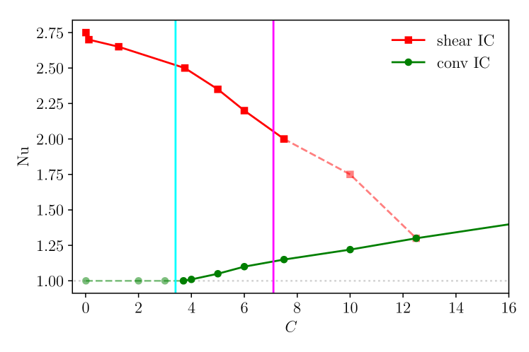
Figure 18: Nusselt number vs $C$ for simulations started with shear and convection initial conditions at $Re=5300$. The magenta and cyan vertical lines correspond to the critical buoyancy parameters $C_{cr,1}$ and $C_{cr,2}$ given by (28) and (31), respectively. For values of $C\gtrapprox C_{cr_{1}}$ ($C\lessapprox C_{cr_{2}}$) the shear-driven (convection-driven) state is not supported and correspondingly the upper (lower) branch is plotted with a dashed semi-transparent line.

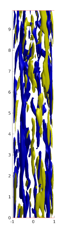
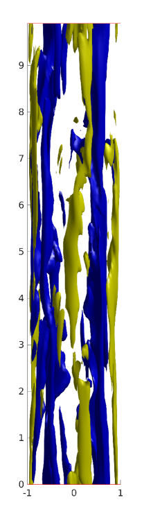
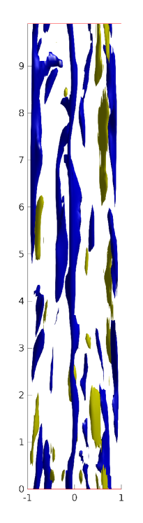
Figure 19: Three-dimensional visualisations of low (blue) and high (yellow) speed streaks in the isothermal (left), heated (middle) and EPG (right) flows. Isosurfaces of turbulent streamwise velocity normalised by the corresponding apparent friction velocity $u_{z}^{\prime}/u_{\tau p}=\pm 4$.

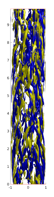
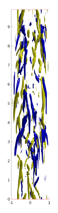
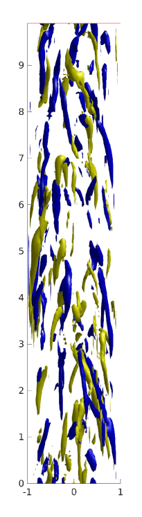
Figure 20: Three dimensional visualisations of vortical structures in the isothermal (left), heated (middle) and EPG (right) flows. Isosurfaces of streamwise vorticity fluctuations normalised by the corresponding apparent friction velocity $\omega_{z}^{\prime}/u_{\tau p}=\pm 35$.

Comparison between the isothermal and heated flows show that the streaks are relatively unaffected, while vortices are significantly weakened. Our interpretation is that while the streaks are responsible for the saturation of the nonlinearity of the flow, via nonlinear normality of the mean flow (Waleffe, 1995), it is relatively ‘easy’ to produce streaks. Note that the mean axial flow for these cases is almost identical (figure 4), and at the end of §3.3 large initial amplifications of disturbances remains possible in the heated case. It is observed that weaker vortices in the heated case are sufficient to produce saturated streaks of the same amplitude. Thus, vortices are more important in the sense that criticality for transition appears to occur when the vortices are too weak. Comparing now the heated flow with the EPG flow, consistent with the observations of HHS (see their figure 19), it can be seen that the streaks in the heated flow are typically stronger than in the EPG flow, while the vortices are of similar strength. In figure 21 we plot RMS velocity fluctuations. Axial perturbations (a) are not strongly affected by the heating, while the cross-flow components (b) are significantly suppressed. (The plot for $u^{\prime}_{r}$ is very similar to that shown for $u^{\prime}_{\theta}$.) In (c) it is seen that the heated and EPG flow have very similar cross-components, while axial perturbations in the heated case are slightly stronger than in the EPG flow. These results are consistent with observations from the three-dimensional visualisations of figures 19 and 20, and likewise suggest that it is the weakening of rolls rather than streaks that appear to be responsible for laminarisation.

(a)                                           (b)

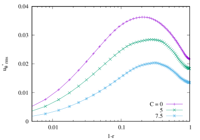
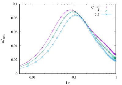
(c)

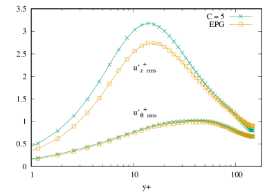
Figure 21: RMS velocity fluctuations. (a) $u^{\prime}_{\theta}$, a measure of ‘rolls’, are suppressed as $C$ increases, while (b) $u^{\prime}_{z}$ a measure of ‘streaks’, are little changed. (c) rolls for the $C=5$ case correspond closely to its EPG counterpart, while the heated case has slightly stronger streaks.

4 Conclusions

In this paper we have studied the flow of fluid through a vertically-aligned heated pipe using direct numerical simulations (DNS), linear stability and nonlinear travelling-wave solution analyses. The flow is driven by an externally applied pressure gradient and aided by the buoyancy resulting from the lightening of the fluid close to the heated wall. DNS were performed for a range of Reynolds numbers $Re$ and buoyancy parameters $C$, where the latter measures the magnitude of the buoyancy force relative to the the pressure gradient of the laminar isothermal shear flow, and three different flow regimes were identified – laminar flow, shear-driven turbulence and convection-driven flow – depending on the flow parameters. At relatively low $Re\lesssim 3500$ turbulence is completely suppressed (relaminarised) by buoyancy and as $C$ is increased convection starts driving a relatively quiescent flow. For larger $Re$, instead, the shear-driven turbulent flow transitions directly to the convection-driven state. Consistent with the appearance of the convective state observed in simulations, a linear instability was found at $C\approx 4$, roughly independent of $Re$ for most of the range considered. The result of increasing $C$ can be compared to that of increasing polymer concentration, or Weissenberg number $Wi$, which is known to have a drag reducing effect on turbulent flows (Virk et al., 1967). Similar to our phase diagram (figure 7), a region of relatively quiescent flow has been reported for a certain range of $Re$ and $Wi$ (Choueiri et al., 2018; Lopez et al., 2019), although the underlying physical mechanism (elastoinertial instability) is clearly very different from the one studied here (convection driven).

Cases where turbulence is suppressed exhibit a flattened mean streamwise velocity profile. In agreement with recent observations by Kühnen et al. (2018) and Marensi et al. (2019) on the effect of flattening, we found that states that mediate turbulence (lower-branch travelling wave solutions) are “pushed out” from the laminar state, i.e. as $C$ increases, a larger perturbation amplitude or larger $Re$ are required to drive shear turbulence until, for sufficiently large $C$, the travelling wave is suppressed altogether.

Finally, we used the relaminarisation criterion recently proposed by He et al. (2016), based on an “apparent Reynolds number” of the flow, to predict the critical $C=C_{cr,1}(Re)$ above which the flow will be laminarised or switch to the convection-driven type. This apparent Reynolds number is based on an apparent friction velocity associated with only the pressure force of the flow (i.e. excluding the contribution of the body force/buoyancy). Bistability between shear or convection-driven states was found to occur in the region $4\lesssim C\lesssim C_{cr,1}$ where the flow may or may not be laminarised depending on the initial flow of the simulation or experiment.

Comparison of the turbulent flow structures (rolls and streaks) with those of two reference flows - the flow of equivalent pressure gradient (EPG) and that of equivalent mass flux (EFR) - suggests that near criticality for relaminarisation the vortices, rather than the streaks, are more important in the sense that criticality for transition occurs when the vortices are too weak. This picture is not straight forward to reconcile with the interpretation of Kühnen et al. (2018), where relaminarisation is attributed to reduced ability to produce streaks in the presence of the flattened base profile. In the heated case, the base velocity profile does not appear to change significantly while shear-driven turbulece is present. Thus it appears unlikely that transient growth of streaks is affected by the heating. Indeed, laminarisation occurs despite little suppression of the streaks. The experiments of Kühnen et al. (2018) are slightly different, however, in that the various flow manipulations they introduce do change the base profile of the flow. In that case it is correct that transient growth will be affected, although we conjecture that it is the suppression of the vortices due to suppression of the streaks that is responsible for laminarisation in that case. Their numerical experiments in the presence of a force are very similar to the calculations here and of HHS. In that case we expect the mechanism we have described to be more clearly responsible for the laminarisation.

Acknowledgments. The anonymous referees are kindly acknowledged for their useful suggestions and comments.

Funding. This work was funded by EPSRC grant EP/P000959/1.

Declaration of Interests. The authors report no conflict of interest.

Appendix A Link between upward-heated and downward-cooled cases

Consider the axial force from the pressure gradient and buoyancy terms in (9). Ignoring the factor $4/Re$ that multiplies all terms, let

$$1+\beta+C\,\Theta=1+\tilde{\beta}+\tilde{C}\,\tilde{\Theta}\,.$$ (33)

with $C>0$ for the upward heated case on the left hand side. Let the right hand side represent the downward cooled case, taking $\tilde{\Theta}=1-\Theta$ so that $\tilde{\Theta}$ is coolest on the boundary ($\tilde{\Theta}=1-r^{2}$ for the laminar case). Put $\tilde{C}=-C<0$, as buoyancy due to positive temperature variations oppose the pressure gradient. (Cooling, however, aids the downward flow.) Substituting in (33) we find $\tilde{\beta}=\beta+C$, i.e. the systems differ only by a known offset in the pressure gradient required to maintain volume flux.

Appendix B Turbulent base flow and eddy viscosity

The turbulent mean flow profile for a pipe may be written $\mbox{\boldmath$U$}=U(y)\hat{\mbox{\boldmath$z$}}$, where $y=1-r$ is the dimensionless distance from the boundary wall and $r$ is the radial coordinate. Applying the Boussinesq eddy viscosity to model for the turbulent Reynolds-stresses, the streamwise component of the Reynolds-averaged momentum conservation reads

$$\frac{1}{Re}\left(\frac{1}{r}+\partial_{r}\right)(\nu_{T}\partial_{r}U)=\partial_{z}P,$$ (34)

where the total effective viscosity is $\nu_{T}(y)=1+\nu_{t}(y)$ and $\nu_{t}$ is the eddy-viscosity, normalised such that $\nu_{T}(0)=1$, i.e. the kinematic value is attained at the wall.

To calculate $\nu_{t}$ it is convenient to use the expression originally suggested for pipe flow by Cess (1958), later used for channel flows by Reynolds & Tiederman (1967) and then by many others (Butler & Farrell, 1993; Del Alamo & Jimenez, 2006; Pujals et al., 2009):

$$\nu_{t}(y)=\frac{1}{2}\left\{1+\frac{\kappa^{2}\hat{R}^{2}\hat{B}}{9}\left(2y-y^{2}\right)^{2}\left(3-4y+2y^{2}\right)^{2}\left[1-e^{\frac{-y\hat{R}\sqrt{\hat{B}}}{A^{+}}}\right]^{2}\right\}^{\frac{1}{2}}-\frac{1}{2}\,.$$ (35)

Here, $\hat{R}=Re\,/\,2$,  $\hat{B}=2\,B$, with $B=-\partial_{z}P$ being the averaged streamwise pressure gradient. The parameters $A^{+}=27$ and $\kappa=0.42$ have been chosen to fit the more recent observations of (McKeon et al., 2005).

For the calculation of §3.4, the (apparent) pressure gradient $B$ and (apparent) $Re_{p}$ are known. The mass flux $Re$ of (34) is not yet known, and we wish to determine $\nu_{t}$. An initial estimate for $Re$ is obtained from the approximation of Blasius (1913), which may be written

$$Re_{p}=\frac{0.0791}{16}\,Re^{1.75}\,.$$ (36)

Then, (35) can be used to calculate $\nu_{t}(r)$, but we must check consistency with (34). The latter equation can be inverted for $U(r)$, and, as it has been non-dimensionalised with the same scales of section §2.1, the mean velocity $U_{b}=2\int_{0}^{1}U(r)\,r\,\mathrm{d}r$ should be $0.5$. It will not be exactly so, as $Re$ (for the given $\partial_{z}P$) has only been estimated. A better estimate is given by $Re:=(0.5/U_{b})\,Re$, so that $\nu_{t}$ can be recalculated and iteratively improved.

References

- Avila et al. (2013) Avila, M., Mellibovsky, F., Roland, N. & Hof, B. 2013 Streamwise-localized solutions at the onset of turbulence in pipe flow. Phys. Rev. Lett. 110, 224502.
- Bae (2016) Bae, Y. Y. 2016 A new formulation of variable turbulent Prandtl number for heat transfer to supercritical fluids. Intl. J. Heat Mass Transfer 92, 792–806.
- Blasius (1913) Blasius, H. 1913 Das ähnlichkeitsgesetz bei reibungsvorgängen in flüssigkeiten. In Mitteilungen über Forschungsarbeiten auf dem Gebiete des Ingenieurwesens, pp. 1–41. Springer.
- Budanur et al. (2017) Budanur, N.B., Short, K.Y., Farazmand, M., Willis, A.P. & Cvitanović, P. 2017 Relative periodic orbits form the backbone of turbulent pipe flow. J. Fluid Mech. 833, 274–301.
- Budanur & Hof (2017) Budanur, Nazmi Burak & Hof, Björn 2017 Heteroclinic path to spatially localized chaos in pipe flow. Journal of Fluid Mechanics 827.
- Butler & Farrell (1993) Butler, K. M. & Farrell, B. F. 1993 Optimal perturbations and streak spacing in wall-bounded turbulent shear flow. Phys.Fluids A 5 (3), 774–777.
- Carr et al. (1973) Carr, AD, Connor, MA & Buhr, HO 1973 Velocity, temperature, and turbulence measurements in air for pipe flow with combined free and forced convection. ASME J. Heat Transfer 95, 445–452.
- Cess (1958) Cess, R. D. 1958 A study of the literature on heat transfer in turbulent tube flow. Tech. Rep.. Tech. Rep. Rep. 8-0529-R24. Westinghouse Research.
- Chantry et al. (2014) Chantry, M., Willis, A. P. & Kerswell, R. R. 2014 Genesis of streamwise-localized solutions from globally periodic traveling waves in pipe flow. Phys. Rev. Lett. 112, 164501.
- Chen & Chung (1996) Chen, Y.-C. & Chung, J. N. 1996 The linear stability of mixed convection in a vertical channel flow. J. Fluid Mech. 325, 29–51.
- Choueiri et al. (2018) Choueiri, G. H., Lopez, J. M. & Hof, B. 2018 Exceeding the asymptotic limit of polymer drag reduction. Phys. Rev. Lett. 120 (12), 124501.
- Del Alamo & Jimenez (2006) Del Alamo, J. C. & Jimenez, J. 2006 Linear energy amplification in turbulent channels. J. Fluid Mech. 559, 205–213.
- Drazin & Reid (2004) Drazin, P. & Reid, W. H. 2004 Hydrodynamic Stability, 2nd edn. Cambridge: Cambridge Univ. Press.
- Duguet et al. (2008) Duguet, Y., Willis, A. P. & Kerswell, R. R. 2008 Transition in pipe flow: the saddle structure on the boundary of turbulence. J. Fluid Mech. 613, 255–274.
- Eckhardt et al. (2007) Eckhardt, B., Schneider, T. M., Hof, B. & Westerweel, J. 2007 Turbulence transition in pipe flow. Ann. Rev. Fluid Mech. 29, 447–468.
- Eggels et al. (1994) Eggels, J. G. M., Unger, F., Weiss, M. H., Westerweel, J., Adrian, R. J., Freidrich, R. & Nieuwstadt, F. T. M. 1994 Fully developed turbulent pipe flow: a comparison between direct numberical simulation and experiment. J. Fluid Mech. 268, 175–209.
- Faisst & Eckhardt (2003) Faisst, H. & Eckhardt, B. 2003 Traveling waves in pipe flow. Phys. Rev. Lett. 91, 224502.
- Graham & Floryan (2021) Graham, Michael D & Floryan, Daniel 2021 Exact coherent states and the nonlinear dynamics of wall-bounded turbulent flows. Annual Review of Fluid Mechanics 53.
- Hanratty et al. (1958) Hanratty, T. J., Rosen, E. M. & Kabel, R. L. 1958 Effect of heat transfer on flow field at low Reynolds numbers in vertical tubes. Ind. & Engng. Chem. 50 (5), 815–820.
- He et al. (2016) He, S., He, K. & Seddighi, M. 2016 Laminarisation of flow at low Reynolds number due to streamwise body force. J. Fluid Mech. 809, 31–71.
- Hof et al. (2010) Hof, B., De Lozar, A., Avila, M., Tu, X. & Schneider, T. M. 2010 Eliminating turbulence in spatially intermittent flows. Science 327 (5972), 1491–1494.
- Hof et al. (2004) Hof, B., van Doorne, C. W. H., Westerweel, J., Nieuwstadt, F. T. M., Faisst, H., Eckhardt, B., Wedin, H., Kerswell, R. R. & Waleffe, F. 2004 Experimental observation of nonlinear traveling waves in turbulent pipe flow. Science 305, 1594–1598.
- Itano & Toh (2001) Itano, T. & Toh, S. 2001 The dynamics of bursting process in wall turbulence. J. Phys. Soc. Japan 70, 701–714.
- Jackson et al. (1989) Jackson, J. D., Cotton, M. A. & Axcell, B. P. 1989 Studies of mixed convection in vertical tubes. Intl J Heat Fluid Flow 10 (1), 2–15.
- Kawahara et al. (2012) Kawahara, G., Uhlmann, M. & van Veen, L. 2012 The significance of simple invariant solutions in turbulent flows. Annu. Rev. Fluid Mech 44, 203–225.
- Kemeny & Somers (1962) Kemeny, G. A. & Somers, E. V. 1962 Combined free and forced-convective flow in vertical circular tubes – experiments with water and oil. Trans. ASME C: J. Heat Transfer 108, 339–346.
- Kerswell (2005) Kerswell, R. R. 2005 Recent progress in understanding the transition to turbulence in a pipe. Nonlinearity 18, R17–R44.
- Kerswell (2018) Kerswell, R. R. 2018 Nonlinear nonmodal stability theory. Annu. Rev. Fluid Mech. 50 (1).
- Kerswell & Tutty (2007) Kerswell, R. R. & Tutty, O.R. 2007 Recurrence of travelling waves in transitional pipe flow. J. Fluid Mech. 584, 69–102.
- Khandelwal & Bera (2015) Khandelwal, M. K. & Bera, P. 2015 Weakly nonlinear stability analysis of non-isothermal Poiseuille flow in a vertical channel. Phys. Fluids 27 (6), 064103.
- Kim et al. (2008) Kim, W. S., He, S. & Jackson, J. D. 2008 Assessment by comparison with dns data of turbulence models used in simulations of mixed convection. Intl J. Heat Mass Transfer 51 (5-6), 1293–1312.
- Kühnen et al. (2018) Kühnen, J., Song, B., Scarselli, D., Budanur, N. B., Riedl, M., Willis, A. P., Avila, M. & Hof, B. 2018 Destabilizing turbulence in pipe flow. Nat. Phys. 14, 386–390.
- Lopez et al. (2019) Lopez, J. M., Choueiri, G. H. & Hof, B.n 2019 Dynamics of viscoelastic pipe flow at low reynolds numbers in the maximum drag reduction limit. J. Fluid Mech. 874, 699–719.
- Marensi et al. (2019) Marensi, E., Willis, A. P. & Kerswell, R. R. 2019 Stabilisation and drag reduction of pipe flows by flattening the base profile. J. Fluid Mech. 863, 850–875.
- McKeon et al. (2005) McKeon, B.J., Zagarola, M.V. & Smits, A.J. 2005 A new friction factor relationship for fully developed pipe flow. J. Fluid Mech. 538, 429–443.
- Nagata (1990) Nagata, M. 1990 Three-dimensional finite-amplitude solutions in plane Couette flow: Bifurcation from infinity. J. Fluid Mech. 217, 519–527.
- Parlatan et al. (1996) Parlatan, Y, Todreas, NE & Driscoll, MJ 1996 Buoyancy and property variation effects in turbulent mixed convection of water in vertical tubes. ASME J. Heat Transfer 118, 381–387.
- Pringle et al. (2009) Pringle, C. C. T., Duguet, Y. & Kerswell, R. R. 2009 Highly symmetric travelling waves in pipe flow. Phil. Trans. Royal Soc. A 367, 457–472.
- Pringle & Kerswell (2007) Pringle, C. C. T. & Kerswell, R. R. 2007 Asymmetric, helical, and mirror-symmetric traveling waves in pipe flow. Phys. Rev. Lett. 99, 074502.
- Pujals et al. (2009) Pujals, G., García-Villalba, M., Cossu, C. & Depardon, S. 2009 A note on optimal transient growth in turbulent channel flows. Phys. Fluids 21 (1), 015109.
- Reynolds & Tiederman (1967) Reynolds, W.C. & Tiederman, W.G. 1967 Stability of turbulent channel flow, with application to malkus’s theory. J. Fluid Mech. 27 (2), 253–272.
- Rogers & Yao (1993) Rogers, B. B. & Yao, L. S. 1993 Finite-amplitude instability of mixed-convection in a heated vertical pipe. Intl. J. Heat Mass Transfer 36 (9), 2305–2315.
- Scheele & Hanratty (1962) Scheele, G. F. & Hanratty, T. J. 1962 Effect of natural convection on stability of flow in a vertical pipe. J. Fluid Mech. 14 (2), 244–256.
- Schmid & Henningson (2001) Schmid, P. J. & Henningson, D. S. 2001 Stability and Transition on Shear Flows, , vol. 142. Springer Science & Business Media.
- Schneider & Eckhardt (2006) Schneider, T. M. & Eckhardt, B. 2006 Edge of chaos in pipe flow. Chaos 16, 041103.
- Schneider et al. (2007) Schneider, T. M., Eckhardt, B. & Yorke, J. 2007 Turbulence, transition, and the edge of chaos in pipe flow. Phys. Rev. Lett. 99, 034502.
- Senoo et al. (2012) Senoo, T., Deguchi, K. & Nagata, M. 2012 Bifurcation of internally heated flow in a vertical pipe. HEFAT 2012 .
- Steiner (1971) Steiner, Alejandro 1971 On the reverse transition of a turbulent flow under the action of buoyancy forces. J. Fluid Mech. 47 (3), 503–512.
- Su & Chung (2000) Su, Y.-C. & Chung, J. N. 2000 Linear stability analysis of mixed-convection flow in a vertical pipe. J. Fluid Mech. 422, 141–166.
- Virk et al. (1967) Virk, P. S., Merrill, E. W., Mickley, H. S., Smith, K. A. & Mollo-Christensen, E. L. 1967 The Toms phenomenon: turbulent pipe flow of dilute polymer solutions. J. Fluid Mech. 30 (2), 305–328.
- Viswanath (2007) Viswanath, D. 2007 Recurrent motions within plane Couette turbulence. J. Fluid Mech. 580, 339–358, .
- Waleffe (1995) Waleffe, F. 1995 Transition in shear flows: Nonlinear normality versus non-normal linearity. Phys. Fluids 7, 3060–3066.
- Waleffe (2001) Waleffe, F. 2001 Exact coherent structures in channel flow. J. Fluid Mech. 435, 93–102.
- Wedin & Kerswell (2004) Wedin, H. & Kerswell, R. R. 2004 Exact coherent structures in pipe flow: Traveling wave solutions. J. Fluid Mech. 508, 333–371.
- White (1979) White, F. M. 1979 Fluid mechanics. Tata McGraw-Hill Education.
- Willis (2017) Willis, A. P. 2017 The Openpipeflow Navier–Stokes solver. SoftwareX 6, 124–127.
- Willis et al. (2013) Willis, A. P., Cvitanović, P. & Avila, M. 2013 Revealing the state space of turbulent pipe flow by symmetry reduction. J. Fluid Mech. 721, 514–540.
- Willis et al. (2010) Willis, A. P., Hwang, Y. & Cossu, C. 2010 Optimally amplified large-scale streaks and drag reduction in turbulent pipe flow. Phys. Rev. E 82, 036321.
- Willis et al. (2016) Willis, A. P., Short, K. Y. & Cvitanović, P. 2016 Symmetry reduction in high dimensions, illustrated in a turbulent pipe. Phys. Rev. E 93, 022204.
- Yao (1987a) Yao, L. S. 1987a Is a fully-developed and non-isothermal flow possible in a vertical pipe? Intl. J. Heat Mass Transfer 30 (4), 707–716.
- Yao (1987b) Yao, L. S. 1987b Linear stability analysis for opposing mixed convection in a vertical pipe. Intl. J. Heat Mass Transfer 30 (4), 810–811.
- Yao & Rogers (1989) Yao, L. S. & Rogers, B. B. 1989 The linear stability of mixed convection in a vertical annulus. J. Fluid Mech. 201, 279–298.
- Yoo (2013) Yoo, J. Y. 2013 The turbulent flows of supercritical fluids with heat transfer. Ann. Rev. Fluid Mechanics 45, 495–525.
- You et al. (2003) You, J., Yoo, J. Y. & Choi, H. 2003 Direct numerical simulation of heated vertical air flows in fully developed turbulent mixed convection. Intl J. Heat Mass Transfer 46 (9), 1613–1627.