fff FISPAC-TH/271/2020 UQBAR-TH/2020-091 Shadows of 5D Black Holes from String Theory

Abstract

We study the shadow behaviors of five dimensional (5D) black holes embedded in type IIB superstring/supergravity inspired spacetimes by considering solutions with and without rotations. Geometrical properties as shapes and sizes are analyzed in terms of the D3-brane number and the rotation parameter. Concretely, we find that the shapes are indeed significantly distorted by such physical parameters and the size of the shadows decreases with the brane or “color” number and the rotation. Then, we investigate geometrical observables and energy emission rate aspects.

Keywords: Black holes, Shadows, D3-branes, Type IIB superstring theory.

1 Introduction

Black holes have been extensively investigated in connections with many gravity theories. Such investigations have been boosted by recent direct observations, the gravitational wave events and by the first image provided by the Event Horizon telescope (EHT) international collaboration [1, 2, 3, 4].

Thermodynamical and optical aspects of numerous black holes, in 4D and arbitrary dimensions, have been dealt with using different approaches and methods including numerical ones [5, 6, 7, 8, 9, 10, 11, 12, 13, 14, 15, 16, 17, 18]. A particular emphasis has been put on black hole objects living in higher dimensions involving various rotating parameters required by space-time symmetries. In such spaces, non-trivial extended black objects can also arise going beyond black holes. The associated horizon geometries have been obtained and examined with using alternative ways.

Many other physical properties have been shown in connections with non-trivial models of gravity in extra dimensions. Specifically, string theory motivated models have been used as playgrounds to study certain phase transitions of black holes in the presence of solitonic D-brane objects. Precisely, the Hawking-Page phase transition of black holes in the $AdS_{5}\times\mathbb{S}^{5}$ geometry have been treated by considering the number of D3-branes as a thermodynamical variable [19]. Such investigations have been extended to M-theory on $AdS_{p+2}\times\mathbb{S}^{11-(p+2)}$ geometries where $p=2$ and 5 [20, 21, 22]. Motivations to consider such higher dimensional frameworks are associated with non-local objects being useful to understand the AdS/CFT conjecture. In particular, explicit examples of such a correspondence are elaborated in many places including [23, 24].

More recently, the shadows and other optical behaviors of the black holes in higher dimensional space-times, motivated by supergravity models, have been investigated. More precisely, 5D black holes involving more than one rotating parameter have been approached using the shadow analysis. A special attention has been devoted to Myers-Perry solutions[25].

The aim of this work is to further advance in the study of properties as the shadows of 5D black holes embedded in type IIB superstring geometries. In particular, we consider solutions without and with rotations. Among other results, we find that the shapes are significantly distorted and the sizes are decreasing with the increase of the D3-brane number and the rotating parameter. The geometrical observables and the energetic aspects are also analyzed in some details.

This work is structured as follows. In section 2, we give a fast review on 5D black holes being embedded in type IIB superstring theory. In section 3, we study the shadows of non-rotating black holes in terms of the D3-branes. In section 4, we investigate a 5D black hole with a single rotating parameter. The geometrical observables and the energetic emission aspects are analyzed in section 5. The last section is devoted to conclusions and open questions.

2 5D rotating type IIB stringy black holes

Let us consider 5D black holes embedded in a type IIB superstring/supergravity geometry with D3-branes. The physics of such solitonic objects has been extensively studied in connections the AdS/CFT conjecture [26, 27, 28]. Properties like the thermodynamical aspects of 5D black holes in such backgrounds have been dealt with by examining certain phase transitions including the Hawking-Page one. Here, we will be interested in optical aspects of such black holes in the $AdS_{5}\times\mathbb{S}^{5}$ physical space. This can be considered as the near horizon geometry of black D3-branes in ten dimensions. Rotating 5D black hole solutions, in general, involve two rotation parameters related to the Casmir operators of the $SO(5)$ Lie group. In this way, non-trivial optical properties depend on such parameters. Following to [28, 29], the metric of a 5D black hole with two rotating parameters assumed to be embedded in the $AdS_{5}\times\mathbb{S}^{5}$ geometry can be written, using Boyer-Lindquist coordinates, as

$$ds^{2} = -{\Delta_{r}\over{\rho}^{2}}\left(dt-{a\sin^{2}{\theta}\over\Xi_{a}}d\phi-{b\cos^{2}{\theta}\over\Xi_{b}}d\psi\right)^{2}+{\rho^{2}\over\Delta_{\theta}}d\theta^{2}+{\Delta_{\theta}\sin^{2}{\theta}\over\rho^{2}}\left(adt-{(r^{2}+a^{2})\over{\Xi}_{a}}d\phi\right)^{2}$$ (2.1)

$$+{(1+r^{2}/\ell_{AdS}^{2})\over r^{2}\rho^{2}}\left(abdt-{b(r^{2}+a^{2})\sin^{2}\theta\over\Xi_{a}}d\phi-{a(r^{2}+b^{2})\cos^{2}\theta\over\Xi_{b}}d\psi\right)^{2}$$

$$+{\rho^{2}\over\Delta_{r}}dr^{2}+{\Delta_{\theta}\cos^{2}{\theta}\over\rho^{2}}\left(bdt-{(r^{2}+b^{2})\over\Xi_{b}}d\psi\right)^{2}+\ell^{2}_{AdS}d\Omega_{5}^{2},$$

where the involved terms are

$$\rho^{2} = r^{2}+a^{2}\cos^{2}\theta+b^{2}\sin^{2}\theta,$$

$$\quad\Xi_{a} = 1-\frac{a^{2}}{\ell_{AdS}^{2}},\quad\Xi_{b}=1-\frac{b^{2}}{\ell_{AdS}^{2}},$$

$$\Delta_{r} = {1\over r^{2}}(r^{2}+a^{2})(r^{2}+b^{2})(1+\frac{r^{2}}{\ell_{AdS}^{2}})-m,$$

$$\Delta_{\theta} = 1-\frac{a^{2}}{\ell_{AdS}^{2}}\cos^{2}\theta-\frac{b^{2}}{\ell_{AdS}^{2}}\sin^{2}\theta.$$ (2.2)

The quantity $m$ is a mass parameter and $a$ and $b$ are the two rotation parameters. The two angular coordinates $\phi$ and $\psi$ are constrained by $0\leq\phi\leq 2\pi$ and $0\leq\psi\leq\pi/2$. $d\Omega_{5}^{2}$ is the metric of the five dimensional sphere $\mathbb{S}^{5}$. From the type IIB superstring/supergravity point of view, the associated ten dimensional factorized spacetime can be interpreted as the near horizon geometry of $N$ coincident configurations of the D3-branes. The AdS radius $\ell_{AdS}$ and the gravitational constant can be related to $N$ via the following relations

$$\ell_{AdS}^{4}=\frac{\sqrt{2}N\ell_{p}^{4}}{\pi^{2}},\qquad G_{5}=\frac{\ell_{p}^{8}}{\pi^{3}\ell_{AdS}^{5}}=\frac{\ell_{p}^{3}}{2^{\frac{5}{8}}\sqrt{\pi}N^{\frac{5}{4}}}.$$ (2.3)

It is noted that the metric Eq.(2.1) is singular when $g_{rr}=\Delta_{r}=0$ and $\rho^{2}=0$. This metric is invariant under the following symmetry

$$a\leftrightarrow b,\quad\theta\leftrightarrow\frac{\pi}{2}-\theta,\quad\phi\leftrightarrow\psi.$$ (2.4)

For the sake of simplicity and to make contact with known results, we will limit our analysis in this work to two cases: zero ($a=b=0$) and one rotation parameter ($b=0$). A more general study will be the object of further investigations left for future works.

3 Shadows of 5D non-rotating black holes in presence of D3-branes

Let us study the null geodesics (test “photon” orbits) around such stringy type IIB black holes. We consider first a baseline case with no rotation. In this case $a=b=0$, the line element in Eq.(2.1) reduces to

$$ds^{2}=-\Delta_{r}dt^{2}+\frac{1}{\Delta_{r}}dr^{2}+r^{2}\left(d\theta^{2}+\sin^{2}\theta d\phi^{2}+\cos^{2}\theta d\psi^{2}\right)+\ell^{2}_{AdS}d\Omega_{5}^{2},$$ (3.5)

where $\Delta_{r}$ is a redefined radial function given by

$$\Delta_{r}=1-\frac{m}{r^{2}}+\frac{r^{2}}{\ell_{AdS}^{2}}.$$ (3.6)

The integration constant $m$ is related to the black hole mass $M$ through the relation

$$m=\frac{8}{3\pi}G_{5}\times M,$$ (3.7)

where $G_{5}$ is the 5D gravitational constant. It is convenient to consider a normalized mass parameter $m^{\prime}=\frac{3\pi}{4}m$. In this way, the above metric becomes

$$\Delta_{r}=1-\frac{2G_{5}M}{r^{2}}+\frac{r^{2}}{\ell^{2}_{AdS}}.$$ (3.8)

In order to implement the D3-brane effect, Eq.(3.8) can be rewritten as (using Eq.(2.3))

$$\Delta_{r}=1-\frac{2^{\frac{3}{8}}M\ell^{3}_{p}}{N^{\frac{5}{4}}\sqrt{\pi}r^{2}}+\frac{\pi r^{2}}{2^{\frac{1}{4}}N^{\frac{1}{2}}\ell^{2}_{p}}.$$ (3.9)

The “photon” orbits or null geodesics of the 5D non-rotating black hole geometry can be computed by using an effective Hamilton-Jacobi approach (see [30, 31], for example, for more detailed calculations). The corresponding Hamilton-Jacobi equation for our case is

$$\frac{1}{2}g^{\mu\nu}\frac{dS}{dx^{\mu}}\frac{dS}{dx^{\nu}}+\frac{dS}{d\tau}=0,$$ (3.10)

where $\tau$ is an affine parameter, and where $S$ is the Jacobian action being given by

$$S=-Et+L_{\phi}\phi+L_{\psi}\psi+S_{r}(r)+S_{\theta}(\theta).$$ (3.11)

$E$, $L_{\phi}$ and $L_{\psi}$ are conserved quantities corresponding to the energy and the angular momentums of the ”photon”, respectively [30]. It is noted that $S_{r}$ and $S_{\theta}$ are functions of $r$ and $\theta$ only, respectively.

Let us use a variable separation method to solve the equation (3.10). Although the use of this method is not strictly necessary in the non-rotating case, it is convenient here to make contact with the rotating case. Separating functions of $r$ and $\theta$, from Eq.(3.10) and Eq.(3.11), we get

$$r^{2}\Delta_{r}\left(\frac{dS_{r}(r)}{dr}\right)^{2}-\frac{r^{2}E^{2}}{\Delta_{r}}+L_{\psi}^{2}+L_{\phi}^{2} = -\mathcal{K}$$ (3.12)

$$\left(\frac{dS_{\theta}(\theta)}{d\theta}\right)^{2}+L_{\phi}^{2}\cot^{2}\theta+L_{\psi}^{2}\tan^{2}\theta = \mathcal{K},$$ (3.13)

where $\mathcal{K}$ is a (real) constant being interpreted as the Carter constant and considered as an additional constant of motion [31]. According to the Hamilton-Jacobi method, we find the following set of equations

$$\frac{dt}{d\tau} = \frac{E}{\Delta_{r}},$$ (3.14)

$$r^{2}\frac{dr}{d\tau} = \pm\sqrt{\mathcal{R}},$$ (3.15)

$$r^{2}\frac{d\theta}{d\tau} = \pm\sqrt{\Theta},$$ (3.16)

$$\frac{d\phi}{d\tau} = \frac{L_{\phi}}{r^{2}\sin^{2}\theta},$$ (3.17)

$$\frac{d\psi}{d\tau} = \frac{L_{\psi}}{r^{2}\cos^{2}\theta},$$ (3.18)

where the terms $\mathcal{R}$ and $\Theta$ are given, respectively, by

$$\mathcal{R} = -\Delta_{r}r^{2}\left(\mathcal{K}+L_{\phi}^{2}+L_{\psi}^{2}\right)+E^{2}r^{4}$$ (3.19)

$$\Theta = \mathcal{K}-L_{\phi}^{2}\cot^{2}\theta-L_{\psi}^{2}\tan^{2}\theta.$$ (3.20)

To get the shadow boundaries, the expression of the effective potential $V_{eff}$ for a radial motion will be needed. Using the relation

$$\left(\frac{dr}{d\tau}\right)^{2}+V_{eff}=0,$$ (3.21)

we obtain the effective potential in such a type IIB stringy solution

$$V_{eff}=\frac{\Delta_{r}}{r^{2}}\left(\mathcal{K}+L_{\phi}^{2}+L_{\psi}^{2}\right)-E^{2}.$$ (3.22)

The unstable circular orbits relying on the maximum of the effective potential are determined by imposing the following constraints

$$V_{eff}=\frac{dV_{eff}}{dr}\Bigm{|}_{r=r_{0}}=0,\qquad\mathcal{R}=\frac{d\mathcal{R}}{dr}\Bigm{|}_{r=r_{0}}=0.$$ (3.23)

Eq.(3.9) can be developed to provide

$$\frac{dV_{eff}}{dr}\Bigm{|}_{r=r_{0}}=-2\frac{\left(\mathcal{K}+L_{\phi}^{2}+L_{\psi}^{2}\right)\left(N^{\frac{5}{4}}\sqrt{\pi}r^{2}-2^{\frac{11}{8}}M\ell_{p}^{3}\right)}{N^{\frac{5}{4}}\sqrt{\pi}r^{5}}=0,$$ (3.24)

where $r_{0}$ is the unstable photon orbit radius. The calculation gives

$$r_{0}=\sqrt{\frac{2^{\frac{11}{8}}M\ell^{3}_{p}}{N^{\frac{5}{4}}\pi^{\frac{1}{2}}}}.$$ (3.25)

Introducing the impact parameters

$$\xi_{1}=\frac{L_{\phi}}{E}\qquad\xi_{2}=\frac{L_{\psi}}{E}\qquad\eta=\frac{\mathcal{K}}{E^{2}},$$ (3.26)

we find the following algebraic geometrical relation

$$E^{2}{r_{0}^{2}-E^{2}\left(\eta+\xi^{2}_{1}+\xi_{2}^{2}\right)\left(1-\frac{2^{\frac{3}{8}}M\ell^{3}_{p}}{N^{\frac{5}{4}}\sqrt{\pi}r_{0}^{2}}+\frac{\pi r_{0}^{2}}{2^{\frac{1}{4}}N^{\frac{1}{2}}\ell^{2}_{p}}\right)}=0.$$ (3.27)

Using Eq.(3.25), this relation can be reformulated as follows

$$\eta+\xi_{1}^{2}+\xi_{2}^{2}=\frac{2^{\frac{19}{8}}M\ell^{3}_{p}\sqrt{N}}{N^{\frac{7}{4}}\sqrt{\pi}+2^{\frac{17}{8}}\pi M\ell_{p}},$$ (3.28)

being a two-dimensional shadow geometry. However, to visualise the corresponding black hole shadows, we introduce the celestial coordinates [32]. Taking the limit of a far away observer, we use such coordinates, considered as a function of the constant of motion

$$\alpha = \lim\limits_{{r_{O}}\rightarrow+\infty}-r_{O}^{2}\left(\sin\theta\frac{d\phi}{dr}+\cos\theta\frac{d\psi}{dr}\right),$$ (3.29)

$$\beta = \lim\limits_{{r_{O}}\rightarrow+\infty}r_{O}^{2}\frac{d\theta}{dr},$$ (3.30)

where $r_{O}$ denotes the distance between the black hole and the observer. Using the expressions

$$\frac{dr}{d\tau}=E\sqrt{1-\frac{\Delta_{r}\left(\eta+\xi_{1}^{2}+\xi_{2}^{2}\right)}{r^{2}}},\qquad\frac{d\theta}{d\tau}=\frac{\sqrt{\mathcal{K}-L_{\phi}^{2}\cot^{2}\theta-L_{\psi}^{2}\tan^{2}\theta}}{r^{2}},$$ (3.31)

we get, for these coordinates, the relations

$$\alpha = -\left(\frac{\xi_{1}}{\sin\theta}+\frac{\xi_{2}}{\cos\theta}\right),$$ (3.32)

$$\beta = \pm\sqrt{\eta-\xi_{1}^{2}\cot^{2}\theta-\xi_{2}^{2}\tan^{2}\theta}.$$ (3.33)

Let us study some particular solutions for the sake of illustration. For instance, we can consider the case when an observer is situated in the equatorial hyperplane in 5D, where the inclination angle is $\theta_{0}=\frac{\pi}{2}$ and $\xi_{2}=0$. Concretely, the shadow geometry for a 5D non-rotating black hole, in the presence of $N$ D3-branes, is characterized by the relation

$$\alpha^{2}+\beta^{2}=\eta+\xi_{1}^{2}=\frac{2^{\frac{19}{8}}M\ell^{3}_{p}\sqrt{N}}{N^{\frac{7}{4}}\sqrt{\pi}+2^{\frac{17}{8}}\pi M\ell_{p}}.$$ (3.34)

To inspect the D3-brane effect, we discuss the shadow behaviors and their radius $R_{c}$ as a function of the D3-brane number $N$. An examination shows that the D3-brane number can be considered a real parameter controlling the involved size. It can be seen clearly that the shadow shape is circular, while the size decreases by increasing the brane number from a maximum value

$$R^{max}_{c}=\frac{2\sqrt[7]{2}\ 5^{5/7}M^{2/7}\ell_{p}^{16/7}}{7\pi^{6/7}},\quad$$ (3.35)

at

$$\quad N^{max}=\frac{2\ 2^{11/14}\pi^{2/7}M^{4/7}\ell_{p}^{4/7}}{5^{4/7}}.$$ (3.36)

The radius decreases with the D3-brane number and it goes to zero in large $N$ limit. In particular, this could also be seen directly from the metric function $\Delta_{r}$. This dependence on the brane number is similar to the one of black hole properties obtained recently in M-theory scenarios [33]. We present a illustration of the results in this non-rotating case in Fig.1.

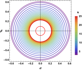
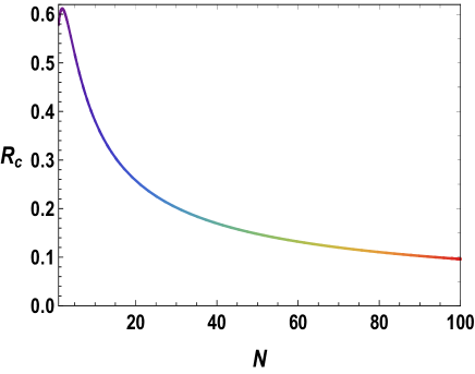
Figure 1: Left: Black hole shadow in the celestial plane $(\alpha-\beta)$ for different values of the brane number $N$ and $\ell_{p}=1,M=1$. Right: The variation of the shadow radius in terms of the branes number $N$. In the left panel, the red circle corresponds to the brane number (N = 100).

Having examined the non-rotating black hole shadows with parallel D3-brane configurations, we will focus in the next section on a more general case by taking into account the rotation effect.

4 Shadows of 5D rotating black holes

We go now beyond the previous results by implementing a single rotating parameter. Taking $b=0$ for simplicity, the line element of a 5D black solution reduces to

$$ds^{2} = -\frac{\Delta_{r}}{\rho^{2}}\left(dt-\frac{a}{\Xi_{a}}\sin^{2}\theta d\phi\right)^{2}+\rho^{2}\left(\frac{dr^{2}}{\Delta_{r}}+\frac{d\theta^{2}}{\Delta_{\theta}}\right)+r^{2}\cos^{2}\theta d\psi^{2}$$

$$+ \frac{\Delta_{\theta}\sin^{2}\theta}{\rho^{2}}\left(adt-\frac{r^{2}+a^{2}}{\Xi_{a}}d\phi\right)^{2}+\ell^{2}_{AdS}d\Omega_{5}^{2},$$

where one has now the following reduced terms

$$\Delta_{r} = (r^{2}+a^{2})(1+\frac{r^{2}}{\ell^{2}_{Ads}})-m,\qquad\Delta_{\theta}=1-\frac{a^{2}}{\ell_{AdS}^{2}}\cos^{2}\theta,$$ (4.38)

$$\rho^{2} = r^{2}+a^{2}\cos^{2}\theta,\qquad\qquad\Xi_{a}=1-\frac{a^{2}}{\ell^{2}_{AdS}}.$$ (4.39)

Using the same Hamilton-Jacobi formalism as in the previous section, we get the following variable separated relations

$$\Delta_{r}\left(\frac{dS_{r}}{dr}\right)^{2}-\frac{\left[E(a^{2}+r^{2})-aL_{\phi}\Xi_{a}\right]^{2}}{\Delta_{r}}+\frac{\left(L_{\phi}\Xi_{a}-aE\right)^{2}}{\Delta_{\theta}}+L_{\psi}^{2}\left(1+\frac{a^{2}}{r^{2}}\right) = -\mathcal{K}$$ (4.40)

$$\Delta_{\theta}\left(\frac{dS_{\theta}}{d\theta}\right)^{2}+\cos^{2}\theta\left(\frac{L_{\phi}^{2}\Xi_{a}^{2}}{\sin^{2}\theta}-a^{2}E^{2}\right)+L_{\psi}^{2}\tan^{2}\theta = \mathcal{K},$$ (4.41)

where the notation is the same as in the previous section. Then, we obtain the geodesic equations

$$\rho^{2}\frac{dt}{d\tau} = \frac{(r^{2}+a^{2})\left[E(r^{2}+a^{2})-aL_{\phi}\Xi_{a}\right]}{\Delta_{r}}+\frac{a(L_{\phi}\Xi_{a}-aE\sin^{2}\theta)}{\Delta_{\theta}},$$ (4.42)

$$\rho^{2}\frac{dr}{d\tau} = \pm\sqrt{\mathcal{R}},$$ (4.43)

$$\rho^{2}\frac{d\theta}{d\tau} = \pm\sqrt{\Theta},$$ (4.44)

$$\rho^{2}\frac{d\phi}{d\tau} = \Xi_{a}\left[\frac{Ea(r^{2}+a^{2})-a^{2}L_{\phi}\Xi_{a}}{\Delta_{r}}+\frac{Ea\sin^{2}\theta-L_{\phi}\Xi_{a}}{\sin^{2}\Delta_{\theta}}\right],$$ (4.45)

$$\frac{d\psi}{d\tau} = \frac{L_{\psi}}{r^{2}\cos^{2}\theta},$$ (4.46)

where $\mathcal{R}$ and $\Theta$ are now given by

$$\Theta = E^{2}\left[\Delta_{\theta}\left(\eta-\xi_{2}^{2}\tan^{2}\theta\right)-\cos^{2}\theta\left(\frac{\xi_{1}^{2}\Xi_{a}^{2}}{\sin^{2}\theta}-a^{2}\right)\right],$$ (4.47)

$$\mathcal{R} = E^{2}\left[\left(a^{2}+r^{2}-a\xi_{1}\Xi_{a}\right)^{2}-\Delta_{r}\left(\frac{\left(a-\xi_{1}\Xi_{a}\right)^{2}}{\Delta_{\theta}}+\eta+\frac{(r^{2}+a^{2})}{r^{2}}\xi_{2}^{2}\right)\right].$$ (4.48)

For $\theta=\frac{\pi}{2}$ and $\psi=\frac{\pi}{2}$ requiring $\xi_{2}=0$, we find immediately the impact parameters

$$\eta = \frac{r^{2}\left[16a^{2}\Delta_{r}-\left(r\Delta^{\prime}_{r}-4\Delta_{r}\right)^{2}\right]}{a^{2}\Delta_{r}^{\prime 2}}|_{r=r_{0}},$$ (4.49)

$$\xi_{1} = \frac{(a^{2}+r^{2})\Delta_{r}^{\prime}-4r\Delta_{r}}{a\Delta_{r}^{\prime}\Xi_{a}}|_{r=r_{0}},$$ (4.50)

where we have used $\Delta^{\prime}_{r}=\frac{\partial\Delta_{r}}{\partial r}$. Exploiting the previous expressions, these impact parameters take the following form

$$\eta = \frac{4\mu\left(a^{2}-\mu\right)-r^{4}\left(a^{2}\nu-1\right)^{2}+4r^{2}\left(a^{2}\mu\nu+\mu\right)}{\left(a^{3}\nu+2a\nu r^{2}+a\right)^{2}},$$ (4.51)

$$\xi_{1} = \frac{a^{4}\nu+a^{2}\nu r^{2}-a^{2}+2\mu-r^{2}}{a^{3}\lambda\nu+a\lambda+2a\lambda\nu r^{2}},$$ (4.52)

where $\mu$, $\nu$, and $\lambda$ are given by

$$\mu=\frac{2^{3/8}\,\ell_{p}^{3}\,M}{\sqrt{\pi}\,n^{5/4}},\hskip 28.45274pt\nu=\frac{\pi}{{2}^{1/4}\,\ell_{p}^{2}\,{n}^{1/2}},\hskip 28.45274pt\lambda=1-\frac{\pi a^{2}}{{2}^{1/4}\,\ell_{p}^{2}\,{n}^{1/2}}.$$ (4.53)

To visualise the associated shadows, we need to introduce the celestial coordinates. For the present model, they are modified as follows

$$\alpha = -\left(\frac{\xi_{1}}{\sin\theta}+\frac{\xi_{2}}{\cos\theta}\right),$$ (4.54)

$$\beta = \pm\sqrt{\eta-\xi_{1}^{2}\cot^{2}\theta-\xi_{2}^{2}\tan^{2}\theta+a^{2}\cos^{2}\theta}.$$ (4.55)

In the equatorial plane $\theta=\frac{\pi}{2}$, these celestial coordinates reduce to

$$\alpha = -\xi_{1},$$ (4.56)

$$\beta = \pm\sqrt{\eta}.$$ (4.57)

A close inspection of Eqs.(4.51,4.52) reveals that the D3-brane number impose strong constraints on the rotating parameter. The possible range of the values of it depends on such a number $N$. This behavior is illustrated in Fig.2 where the parametric curves $(\alpha(r),\beta(r))$ are shown for a set of fixed parameters $a$ and $N$. To get significant shadows as functions of the rotation parameter $a$, we should consider $N$ lower than a certain number (less than $\approx 8$ in the case of the illustrating figure).

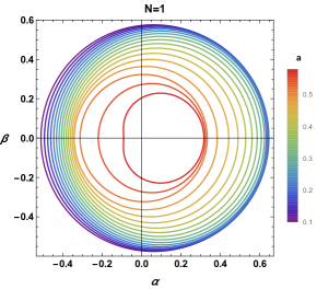
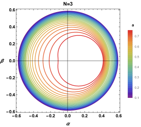
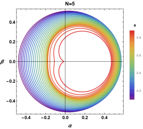
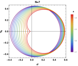
Figure 2: Shadow geometry of a rotating AdS black hole for different values of the brane number $N$ and the rotating rate $a$ (for $\ell_{p}=1$ and $M=1$).

Fixing the D3-brane number, one observes that the shadow size decreases by increasing the rotating parameter $a$. For $N=1$, the shadows keep the circular behaviors for small values of $a$. For $N>1$, however, the shadow starts developing a D-form for the high values of the rotation parameter near $a\simeq 0.7$. As the number of the D3-branes increases the D-shape becomes of “cardioid” type. Similar effects were firstly uncovered in [16]. This complicated geometry has been shown to appear either in M-theory scenarios in the presence of the M2-branes [33] or in charged rotating black holes with a cosmological constant [16]. Let us finally note that the black hole shadow is controlled basically by three parameters $(M,N,a)$ namely a moduli space. Not all regions in such a space are acceptable.

5 Geometrical observable and energy emission rate aspects

In this section, we discuss further geometrical observables and the behavior of the black hole energy emission rate as a function of the brane number and the rotation. The observation of the shadow of the supermassive black hole $M87^{\star}$ has opened a promising to probe gravity theories beyond GR, in particular candidates to quantum gravity as M-theory [33] or string theory (as in the present work). We show next that the present or near-future observational data is indeed sensitive to stringy brane effects, i.e. through $N$, the number of D3-branes, and, it potentially could be used to put constraints on the black hole parameters and then on the string theory itself.

Geometrical physical observables

We approach now the study of observables which can be useful for making contact with present or future black hole observations. To get geometrical physical data, one needs two observables. They are for example the radius $R_{c}$ of the shadow and the distortion $\delta$ controlling the size and shape respectively. Before going ahead, let us briefly recall the definition of them. To facilitate the discussion, we consider shadow configurations with $\xi_{2}=0$ as in the previous section. Following [34], the shadow of the black hole is characterized by three specific points. They are the top and the bottom positions ($\alpha_{t},\beta_{t}$), ($\alpha_{b},\beta_{b}$) respectively, and the point of a standard circle ($\alpha_{p},0$). The point of the distorted shadow circle ($\alpha_{p},0$) intersects the horizontal axis at $\alpha$. The distance between the two points is controlled by the parameter

$$D=2R_{c}-(\alpha_{r}-\alpha_{p}).$$ (5.58)

Following to [35], it has been shown that the parameter $R_{c}$ of shadows takes the following form

$$R_{c}=\frac{(\alpha_{t}-\alpha_{r})^{2}+\beta_{t}^{2}}{2|\alpha_{t}-\alpha_{r}|}.$$ (5.59)

The distortion parameter is characterized by the ratio of $D_{c}$ and $R_{c}$

$$\delta_{c}=\frac{D}{R_{c}}.$$ (5.60)

These geometrical quantities will be discussed graphically. The associated calculations are illustrated in Fig.3.

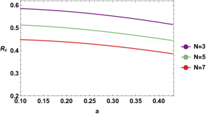
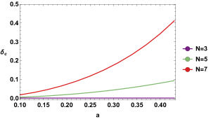
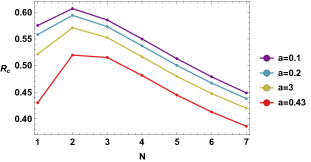
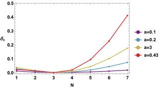
Figure 3: Astronomical observation variables for different values of the brane numbers $N$, the rotating rate $a$, for $\ell_{p}=1$ and $M=1$.

One observes from the figure that, at fixed brane number $N$, the size of the shadow $R_{c}$ decreases by the increase of the rotation parameter $a$. For the distortion parameter, however, $\delta_{c}$ increases by increasing the rotation parameter $a$. It is also noted that $\delta_{c}$ is almost null for $N\simeq 3$. When fixing the rotation $a$, the quantity $R_{c}$ increases with the D3-brane number to reach a maximum and then it decreases. However, the distortion parameter $\delta_{c}$ decreases to reach a vanishing value then it increases gradually within increasing $N$. As it is shown in the previous section, both parameters $R_{c}$ and $\delta_{c}$ are not always defined and are sensible to a selective value of the moduli space spanned by the triplet $(M,N,a)$.

Energy emission rates

Here, we focus on the energy emission rate. Indeed, for a far distant observer the high energy absorption cross section approaches to the geometrical optical limit, the black hole shadow. In intermediate regimes, the absorption cross section of the black hole oscillates around limiting constant value $\sigma_{lim}$ at very high energy[36, 37]. This limiting constant value, being approximately equal to the size of “photon” 3-sphere. In this approximation, the energy emission rate can be written as

$$\frac{d^{2}E(\omega)}{d\omega dt}=\frac{2\pi^{2}\sigma_{lim}}{e^{\frac{\omega}{T_{{out}}}}-1}\omega^{4},$$ (5.61)

where $\omega$ is the emission frequency, $R_{c}$ is the shadow radius and $T_{out}$ is the Hawking temperature of the black hole. In five dimensional space-time, it is recalled that $\sigma_{lim}$ is approached as

$$\sigma_{lim}\approx\frac{\pi^{3/2}R_{c}^{3}}{\Gamma(\frac{5}{2})}$$ (5.62)

providing

$$\frac{d^{2}E(\omega)}{d\omega\,dt}=\frac{8\pi^{3}\,\,R^{3}_{c}}{3(e^{\frac{\omega}{T_{out}}}-1)}\omega^{4}.$$ (5.63)

In this case, the temperature $T_{out}$ can be expressed as

$$T_{out}=\frac{r_{h}}{\pi(r_{h}^{2}+a^{2})}\left(1+\frac{(2r_{h}^{2}+a^{2})}{2^{1/4}\ell_{p}^{2}\,\sqrt{N}}\right),$$ (5.64)

where $r_{h}$ is the horizon radius. We show the illustrate the behavior of the energy emission rate versus the frequency for different values of the rotation parameter and the brane number in Fig.4.

One observes from the formula, and is graphically clear in the figure, that the energy emission rate varies only slowly. The peak of the energy emission rate slowly shifts to lower frequencies and its height decreases with the increase in the values of the rotation parameter. This behavior is similar to what happens to black holes embedded in M-theory compactifications[33]. Finally we note that increasing the D3-brane number, the energy emission rate vanishes by increasing the rotating parameter.

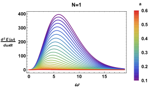
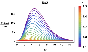
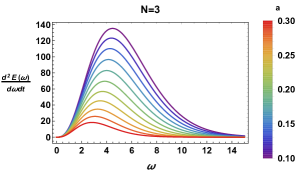
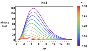
Figure 4: Emission rate of the $AdS_{5}\times\mathbb{S}^{5}$ black hole for different values of the rotation parameter $a$ and the brane numbers $N$, for $\ell_{p}=1$ and $M=1$.

6 Further discussions and conclusions

In this work, we have investigated the shadow properties of 5D black holes embedded in type IIB superstring/supergravity inspired spacetimes. In particular, we have studied the effect of the presence of an arbitrary number of D3-branes and of the rotation on the shape and size of the shadows. For non-rotating solutions, the circular size of the shadow decreases with the D3-brane number. Larger values of the rotation parameter decrease, however, the size of the shadows. This behavior matches the “intuitive” idea indicating that when the black hole rotates rapidly, null geodesics or “photon” orbits become closer due to a decreasing in the effective gravitational effects. After that, we have analyzed the geometrical observables associated with the distortion and the size of the shadows, respectively. Among others, we have found that the shapes are significantly more and more distorted and the size is decreasing with the D3-brane number and the rotating parameter. The energy emission rate aspects of such 5D black holes have been examined in some details. It has been remarked that the obtained behavior is similar to the one observed in M-theory black holes [33]. This work opens up for further studies. One interesting question is to complete this analysis by considering the general case where the two rotating parameters supported by the $SO(5)$ Lie symmetry are switched on. In particular, it is interesting to write down the associated shadow geometries. A natural question concerns the extension of this work to the case of external sources involving either dark energy or dark matter. We hope to report elsewhere on these open questions in future [38].

References

- [1] B. Abbott et al., Observation of Gravitational Waves from a Binary Black Hole Merger, Phys. Rev. Lett. 116(6)(2016)061102, arXiv:1602.03837.
- [2] K. Akiyama et al., First M87 Event Horizon Telescope Results. IV. Imaging the Central Supermassive Black Hole, Astrophys. J. L4(1)(2019)875, arXiv:1906.11241.
- [3] K. Akiyama et al., First M87 Event Horizon Telescope Results. V. Imaging the Central Supermassive Black Hole, Astrophys. J. L5(1)(2019)875.
- [4] K. Akiyama et al., First M87 Event Horizon Telescope Results. VI. Imaging the Central Supermassive Black Hole, Astrophys. J. L6(1)(2019)875.
- [5] D. Kubiznak, R. B. Mann, P-V criticality of charged AdS black holes, JHEP 1207 (2012) 033.
- [6] S. Hawking, D. N. Page, Thermodynamics of Black Holes in anti-De Sitter Space, Commun. Math. Phys. 87 (1987) 577.
- [7] A. Chamblin, R. Emparan, C. Johnson, R. Myers, Charged AdS black holes and catastrophic holography, Phys. Rev. D60 (1999) 064018.
- [8] A. Belhaj, M. Chabab, H. El Moumni, M. B. Sedra, On Thermodynamics of AdS Black Holes in Arbitrary Dimensions, Chin. Phys. Lett. 29 (2012) 100401.
- [9] P. V. Cunha, C. A. Herdeiro, E. Radu, H. F. Runarsson, Shadows of Kerr black holes with and without scalar hair, Inter. Jour. Mod. Phys. D (2016) 25 1641021.
- [10] K. S. Virbhadra, G. F. Ellis, Schwarzschild black hole lensing, Phys. Rev. D62(8)(2000)084003.
- [11] P.-C. Li, M. Guo, B. Chen, Shadow of a spinning black hole in an expanding universe, Phy. Rev. D101(8)(2020)084041.
- [12] S-F. Yan, C. Li, L. Xue, X. Ren, Y-F. Cai, D. A. Easson, Y-F Yuan, H. Zhao, Testing the equivalence principle via the shadow of black holes, Phys. Rev. Res. 2(2020) 023164, arXiv:1912.12629.
- [13] A. Belhaj, A. El Balali, W. El Hadri, H. El Moumni, M. B. Sedra, Dark energy effects on charged and rotating black holes, Eur. Phys. J. Plus 134(9) (2019) 422.
- [14] A. Belhaj, A. El Balali, W. El Hadri, M. A. Essebani, M. B. Sedra, A. Segui, Kerr-AdS Black Hole Behaviors from Dark Energy, Int. Jour. of Mod. Phys. D29 (09) (2020) 2050069.
- [15] C. Goddi et al., BlackHoleCam: Fundamental physics of the galactic center, Int. J. Mod. Phys. D. 26(4)(2016)1730001, arXiv:1606.08879.
- [16] A. Belhaj, M. Benali, A. El Balali, W. El Hadri, H. El Moumni, Shadows of Charged and Rotating Black Holes with a Cosmological Constant, (2020), arXiv:2007.09058.
- [17] B. Indrani, C. Sumanta, S. Soumitra, Silhouette of M87*: A New Window to Peek into the World of Hidden Dimensions, Phys. Rev. D. 101(4)(2020)041301, arXiv:1909.09385.
- [18] A. Belhaj, L. Chakhchi, H. El Moumni, J. Khalloufi, K. Masmar, Thermal Image and Phase Transitions of Charged AdS Black Holes using Shadow Analysis, arXiv:2005.05893.
- [19] J. L. Zhang, R. G. Cai, H. Yu, Phase transition and thermodynamical geometry for Schwarzschild AdS black hole in spacetime, J. High Ener. Phys. 2 (2015) 143.
- [20] A. Belhaj, M. Chabab, H. El Moumni, K. Masmar, M. Sedra, On Thermodynamics of AdS Black Holes in M-Theory, Eur. Phys. J. C. 76(2)(2016)73, arXiv:1509.02196.
- [21] M. Chabab, H. El Moumni, K. Masmar, On thermodynamics of charged AdS black holes in extended phases space via M2-branes background, Eur. Phys. J. C. 76(6)(2016)304, arXiv:1512.07832.
- [22] A. Belhaj, A. E. Balali, W. E. Hadri, Y. Hassouni, E. Torrente-Lujan, Phase Transitions of Quintessential AdS Black Holes in M-theory/Superstring Inspired Models, arXiv:2004.10647.
- [23] A. M. Awad, C. V. Johnson, Higher dimensional Kerr - AdS black holes and the AdS / CFT correspondence, Phys. Rev. D 63 (2001) 124023, arXiv:hep-th/0008211.
- [24] K. Nagasaki, H. Tanida, S. Yamaguchi, Holographic Interface-Particle Potential, JHEP 01 (2012) 139, arXiv:1109.1927.
- [25] P. Uma, A. Farruh, G. G. Sushant, A. Bobomurat, Shadow of five-dimensional rotating Myers-Perry black hole, Phys. Rev. D. 90(2)(2014)024073, arXiv:1407.0834.
- [26] J. M. Maldacena, A. Strominger, E. Witten, Black hole entropy in M theory, High Energy Phys. 1997(12)(1998)002, arXiv:hep-th/9711053.
- [27] V. R. Alfonso, Introduction to the AdS/CFT correspondence, arXiv:1310.4319.
- [28] A. M. Adel, V. J. Clifford, Higher dimensional Kerr-AdS black holes and the AdS/CFT correspondence, Phys. Rev. D. 63(12)(2001)124023, arXiv:hep-th/0008211.
- [29] S. W. Hawking, C. J. Hunter, M. M. TaylorRobinson, Rotation and the AdS/CFT correspondence, Phys. Rev. D59 (1999) 064005, hep-th/9811056.
- [30] S. Chandrasekhar, The mathematical theory of black holes, Oxford University Press. 69(1998).
- [31] B. Carter, Global structure of the Kerr family of gravitational fields, Phys. Rev. 174(5)(1968)1559.
- [32] M. Amir, B. P. Singh, S. G. Ghosh, Shadows of rotating five-dimensional charged EMCS black holes, Eur. Phys. J. C78 no.5 (2018) 399, arXiv:1707.09521.
- [33] A. Belhaj, M. Benali, A. E. Balali, W. E. Hadri, H. El Moumni, E. Torrente-Lujan, Black Hole Shadows in M-theory Scenarios, arXiv:2008.09908 [hep-th].
- [34] H. Kenta, K-i. Maeda, Measurement of the Kerr spin parameter by observation of a compact object’s shadow, Phys. Rev. D. 80(2)(2009)024042, arXiv:0904.3575.
- [35] A. Muhammed, G. G. Sushant, Shapes of rotating nonsingular black hole shadows, Phys. Rev. D. 94(2)(2016)024054, arXiv:1603.06382.
- [36] S-W. Wei, X-Y. Liu, Observing the shadow of Einstein-Maxwell-Dilaton-Axion black hole, JCAP. 2013(11)(2013)063, arXiv:1311.4251.
- [37] A. Belhaj, M. Benali, A. El Balali, H. El Moumni, S-E. Ennadifi, Deflection Angle and Shadow Behaviors of Quintessential Black Holes in arbitrary Dimensions, arXiv:2006.01078.
- [38] A. Belhaj et al. Work in progress.