Three-dimensional quantum Hall effect and magnetothermoelectric properties in Weyl semimetals

Abstract

We numerically study the three-dimensional (3D) quantum Hall effect (QHE) and magnetothermoelectric transport of Weyl semimetals in the presence of disorder. We obtain a bulk picture that the exotic 3D QHE emerges in a finite range of Fermi energy around the Weyl points determined by the gap between the $n=-1$ and $n=1$ Landau levels (LLs). The quantized Hall conductivity is attributable to the chiral zeroth LLs traversing the gap, and is robust against disorder scattering for an intermediate number of layers in the direction of the magnetic field. Moreover, we predict several interesting characteristic features of the thermoelectric transport coefficients in the 3D QHE regime, which can be probed experimentally. This may open a new avenue for exploring Weyl physics in topological materials.

I Introduction

Weyl semimetals have been attracting intense interests in recent years Wan2011 ; Weng2015 ; Lv2015 ; Jiang2015 ; Chen2015 ; Nielsen ; Huang2015 ; Xu2015 ; Lv15 ; Yang2015 . The band touching points known as the Weyl points always appear in pairs with the opposite chirality Nielsen , and act like magnetic monopoles in momentum space with quantized Berry flux. Another prominent feature of Weyl semimetals is the existence of topologically protected surface states. These surface states in momentum space form nonclosed Fermi arc, connecting the Weyl points projected to the surface Brillouin zone. Due to these unique features, Weyl semimetals exhibit many exotic quantum transport properties, such as chiral anomaly Nielsen ; yang2011 ; Vazifeh2013 ; Parameswaran2014 , the accompanying negative magnetoresistance Son2013 ; Burkov2014 ; Lu2015 , and the planar Hall effect Nandy2017 ; Burkov2017 ; Kumar2018 ; Yang2019 . In particular, the three-dimensional (3D) quantum Hall effect (QHE) is predicted to occur in Weyl semimetals, where the Fermi arcs at opposite surfaces can form a complete Fermi loop and support the QHE by a “wormhole” tunneling between the Weyl points Wang2017 ; Lu2019 ; Sun2019 . As it is well known, 3D systems normally do not exhibit the QHE owing to the continuum spectrum from the band dispersion along the direction of the magnetic field. Therefore, such an intriguing transport signature of Weyl semimetals has attracted more research to reveal the physics of the 3D QHE Zhang2017 ; Zhang2019 ; Lin2019 ; Uchida2017 ; Gao2018 ; Li2020 . Experimentally, the 3D QHE was observed in Dirac semimetal ZrTe₅ crystals Tang2019 , and a charge-density-wave mechanism of the 3D QHE is also proposed to explain experimental observations Qin2020 . However, the interplay between the system sizes, the magnetic field strength and the disorder scattering effect of the 3D QHE in Weyl semimetals have not been understood.

Another exciting frontier is to explore the thermoelectric transport of Weyl semimetals, due to the possibility of record-high thermoelectric conversion efficiency in these semimetal systems  Caglieris2018 ; Watzman2018 ; Hirschberger2016 ; Chen2016 ; Gooth2017 ; Sharma2016 ; Gorbar2017 ; Yang18 ; Jia2016 . More recently, a nonsaturating thermopower and quantized thermoelectric Hall conductivity has been proposed for Weyl semimetals Fu1904 ; Skinner2018 ; Fu2019 . Although there has been much work on the thermoelectric transport properties, thermoelectric transport in the 3D QHE regime and the effect of the disorder scattering have not been studied. Such an investigation is highly desired.

In this paper, we report a numerical study of the QHE and magnetothermoelectric transport of a 3D Weyl semimetal in the presence of disorder. We demonstrate that the Hall conductivity $\sigma_{xy}$ exhibits well-defined plateaus in units of $e^{2}/h$ for electron Fermi energy in the finite gap $E_{g}$ ($E_{g}=2\sqrt{2}\hbar\omega_{c}$ with $\omega_{c}$ as the cyclotron frequency) between the $n=-1$ and $n=1$ Landau levels (LLs) around the Weyl points, as the zeroth LLs are discretized for an intermediate number of layers in the direction of the magnetic field. Our theory suggests a new version of QHE protected by bulk energy gap, which may occur in the 3D Weyl semimetal, and is different from the 3D QHE based on “wormhole” tunneling proposed in Refs.21-23. We show how the system size, the magnetic field strength and disorder influence the quantized Hall plateaus. We further reveal that the transverse thermoelectric conductivity $\alpha_{xy}$ develops a plateau for a wide range of temperatures, which is quantized at an universal constant signaling the LL quantization. The Nernst signal $S_{xy}$ shows a broad maximum at intermediate $T$ for strong magnetic fields, which shifts to lower $T$ with decreasing magnetic field strength. Our work provides a systematical understanding of the topological 3D QHE and magnetothermoelectric transport in Weyl semimetals.

This paper is organized as follows. In Sec. II, the model Hamiltonian of the 3D Weyl semimetal is introduced. In Sec. III, numerical results of the quantized Hall conductivity and thermoelectric transport coefficients obtained by using exact diagonalization are presented. The final section contains a summary.

II Model and Methods

Let us start from a minimal two-band model of Weyl semimetals on a 3D cubic lattice, whose Hamiltonian in momentum space is given by Armitage2018

$$H = t_{x}(\sin k_{x}a)\sigma_{x}+t_{y}(\sin k_{y}a)\sigma_{y}$$ (1)

$$+ (M_{1}-t_{x}\cos k_{x}a-t_{y}\cos k_{y}a-t_{z}\cos k_{z}a)\sigma_{z},$$

where $a$ is the lattice constant, and $t_{i}$ ($i=x,y,z$) denotes the hopping integral along the $i$ axis. $\mbox{\boldmath{$\sigma$}}=(\sigma_{x},\sigma_{y},\sigma_{z})$ is the Pauli matrices for the pseudospin orbital degrees of freedom. ${\bf k}=(k_{x},k_{y},k_{z})$ is the wave vector, and $M_{1}$ is the effective Zeeman strength. For $|(M_{1}-t_{x}-t_{y})/t_{z}|<1$, as considered here, a pair of Weyl points are located at ${\bf k_{\pm}}=(0,0,\pm k_{0})$ with $\cos(k_{0}a)=(M_{1}-t_{x}-t_{y})/t_{z}$. Expanding Eq. (1) around the two Weyl points, one can obtain the corresponding low-energy effective Hamiltonian $H=\hbar v_{F}^{x}\sigma_{x}q_{x}+\hbar v_{F}^{y}\sigma_{y}q_{y}\pm\hbar v_{F}^{z}\sigma_{z}q_{z}$, where $\pm$ are for the two Weyl valleys, and ${\bf q}={\bf k}-{\bf k}_{\pm}$ are the relative wave vectors. $v_{F}^{x}=t_{x}a/\hbar$, $v_{F}^{y}=t_{y}a/\hbar$, and $v_{F}^{z}=t_{z}a\sin(k_{0}a)/\hbar$ are the Fermi velocities.

In real space, when a homogeneous magnetic field ${\bf B}=(0,0,B)$ is applied along the $z$ direction, the tight-binding Hamiltonian on the cubic lattice corresponding to Eq. (1) can be written as  Gao2018 ,

$$H = \sum\limits_{\langle{nml}\rangle}C_{n+1,m,l}^{\dagger}T_{x}C_{n,m,l}+e^{n(2\pi\phi i)}C_{n,m+1,l}^{\dagger}T_{y}C_{n,m,l}$$ (2)

$$+ C_{n,m,l+1}^{\dagger}T_{z}C_{n,m,l}+\frac{M_{1}}{2}C_{n,m,l}^{\dagger}\sigma_{z}C_{n,m,l}$$

$$+ w_{n,m,l}C_{n,m,l}^{\dagger}C_{n,m,l}+H.c.\ .$$

Here, the summation of $\langle{nml}\rangle$ runs over all lattice sites. $C_{n,m,l}^{\dagger}=(C_{n,m,l,\uparrow}^{\dagger},C_{n,m,l,\downarrow}^{\dagger})$ is the two-component creation operators of electrons on the lattice site with coordinates $(n,m,l)$ along the ${x,y,z}$ direction, respectively. $T_{x}=-\frac{1}{2}t_{x}(i\sigma_{x}+\sigma_{z})$, $T_{y}=-\frac{1}{2}t_{y}(i\sigma_{y}+\sigma_{z})$ and $T_{z}=-\frac{1}{2}t_{z}\sigma_{z}$ denote the $2\times 2$ hopping matrices along the three directions, respectively. $\phi$ stands for the magnetic flux per square in units of flux quantum $\phi_{0}=h/e$, namely, $\phi=Ba^{2}/\phi_{0}$. The magnetic field strength $B$ is determined by $B=\phi\phi_{0}/a^{2}$. Since we focus on the low-energy or equivalently long-wavelength properties of the model, the results are insensitive to the lattice structure. In order to obtain a realistic magnetic field $B$, we may choose a relatively large lattice constant $a$. For example, we choose $a=20\AA$, and then $\phi=1/192$ corresponds to $B\simeq 6$ Tesla. In the following numerical calculations, the hopping parameters are chosen to be $t_{x}=t_{y}=t_{z}=t$, and $M_{1}=t_{x}+t_{y}+0.6t_{z}$. The last term is the on-site random potential accounting for disorder scattering, where $w_{n,m,l}$ is uniformly distributed in the range $w_{n,m,l}\in[-W/2,W/2]$, with $W$ as the disorder strength Huo1992 ; Sheng1997 .

In the linear response regime, the charge current in response to an electric field and a temperature gradient can be written as ${\bf J}={\hat{\sigma}}{\bf E}+{\hat{\alpha}}(-\nabla T)$, where ${\hat{\sigma}}$ and ${\hat{\alpha}}$ are the electrical and thermoelectric conductivity tensors, respectively. The electrical conductivity $\sigma_{ij}$ at zero temperature can be calculated by using the Kubo formula Wang2017

$$\sigma_{ij}=\frac{ie^{2}\hbar}{S}\sum_{{\epsilon_{\alpha}}\neq{\epsilon_{\beta}}}\frac{f(\epsilon_{\alpha})-f(\epsilon_{\beta})}{\epsilon_{\alpha}-\epsilon_{\beta}}\frac{\langle\alpha\mid V_{i}\mid\beta\rangle\langle\beta\mid V_{j}\mid\alpha\rangle}{\epsilon_{\alpha}-\epsilon_{\beta}+i\eta}.$$ (3)

Here, $i,j=x,y$, and $\epsilon_{\alpha}$ and $\epsilon_{\beta}$ are the eigenenergies corresponding to the eigenstates $|\alpha\rangle$ and $|\beta\rangle$ of the system, respectively, which can be obtained through exact diagonalization of the Hamiltonian Eq. (2). $S$ is the cross-section area in the $x$-$y$ plane. $f(\epsilon_{\alpha})$ and $f(\epsilon_{\beta})$ are the Fermi-Dirac distribution functions, defined as $f(x)=1/[e^{(x-E_{F})/k_{B}T}+1]$. $V_{i}$ and $V_{j}$ are the velocity operators, and $\eta$ is the positive infinitesimal. The Hall conductivity $\sigma_{xy}$, as the summation of contributions from all layers, has a dimension of $e^{2}/h$.

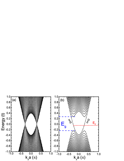
Figure 1: (color online). The energy dispersion as a function of the wave vector $k_{z}$ with a periodic boundary condition for a 3D Weyl semimetal. (a) $\phi=0$, (b) $\phi=1/192$. The system size in the $x$ direction is taken to be $n_{x}=192$. The zeroth Landau levels (LLs) are labeled by $n=0$. The gap between $n=-1$ and $n=1$ LLs is labeled as $E_{g}$. The Weyl point is set as zero of the energy.

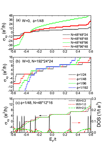
Figure 2: (color online). Calculated Hall conductivities $\sigma_{xy}$ near the band center in Weyl semimetal. (a) For the system size dependence of $\sigma_{xy}$. Here, the magnetic flux is chosen as $\phi=1/48$. (b) For the magnetic field dependence of $\sigma_{xy}$. Here, the system size is fixed at $N=192\times 24\times 24$, the magnetic flux is chosen as $\phi=1/24$, $1/48$, $1/96$ and $1/192$, respectively. In (a) and (b), the disorder strength is set to $W=0$. (c) For the disorder effect on $\sigma_{xy}$ and DOS. The disorder strength is chosen to be $W/t=0.2$, $1.0$ and $2.0$, respectively. The system size is taken to be $N=48\times 12\times 16$, and the magnetic flux is chosen as $\phi=1/48$.

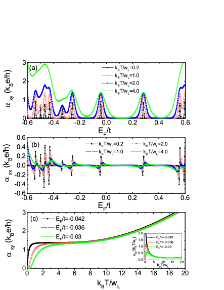
Figure 3: (color online). Thermoelectric conductivities at finite temperatures. (a) $\alpha_{xy}$, (b) $\alpha_{xx}$ as functions of the Fermi energy at different temperatures. (c) shows the temperature dependence of $\alpha_{xy}$ for certain fixed Fermi energies. The inset shows $\alpha_{xy}/(k_{B}T/W_{L})$ as a function of the temperature. Here, $W_{L}$ is chosen as $W_{L}/t=0.005$, the system size is chosen as $N=48\times 12\times 16$, the disorder strength is set to $W/t=0.2$, and the magnetic flux is chosen as $\phi=1/48$.

III Results and Discussion

III.1 Quantized Hall conductivity

We first present the energy dispersion with a periodic boundary condition in the 3D Weyl semimetal. As shown in Fig. 1(a), in the absence of a magnetic field, the conduction and valence bands touch each other at a pair of Weyl points $k_{z}=\pm k_{0}$. Around these Weyl points the energy dispersion is linear. When a perpendicular magnetic field is applied, as shown in Fig. 1(b), the energy spectrum is quantized into the continuum LLs, except for the chiral zeroth LLs (the curve labeled by $n=0$), which are separating from the continuum spectrum. The $n=0$ LLs are apparently discretized, because $k_{z}$ is quantized owing to the finite thickness $n_{z}a$ in the $z$ direction. The energy spacing between two neighboring $n=0$ LLs is approximately given by $\Delta E=v_{F}^{z}\hbar(2\pi/n_{z}a)=2\pi t\sin(k_{0}a)/n_{z}$ inversely proportional to the thickness $n_{z}a$, which will determine the width of the quantized Hall plateaus.

We now present the Hall effect of Weyl semimetals at zero temperature in the presence of a perpendicular magnetic field. In Fig. 2(a), the Hall conductivities $\sigma_{xy}$ are plotted as functions of the electron Fermi energy $E_{F}$ for a clean sample $W=0$ with different system sizes at the same magnetic flux $\phi=1/48$. $\sigma_{xy}$ shows a series of relatively wide quantized Hall plateaus in units of $e^{2}/h$, as long as $E_{F}$ is in the gap between $n=-1$ and $n=1$ LLs of width about $E_{g}=2\sqrt{2}\hbar\omega_{c}=2\sqrt{2}\hbar v_{F}/l_{B}$, with $l_{B}=\sqrt{\hbar/{eB}}$ as the magnetic length deng2019 . For the hopping parameters chosen, the Fermi velocities in the $x$-$y$ plane are isotropic, so we denote $v_{F}^{x}=v_{F}^{y}=v_{F}$. The gap $E_{g}$ has been indicated in Fig. 1(b). For $\phi=1/48$, $E_{g}=2\sqrt{2}\hbar v_{F}/\sqrt{\hbar/{eB}}=4\sqrt{\pi\phi}t\simeq 1.0t$. Outside the gap $E_{g}$, we see much narrower plateaus, originating from energetically overlapped multiple LL subbands, which are unstable when we turn on the random disorder. The quantized Hall conductivity displays a pronounced electron-hole asymmetry due to the asymmetry of the band structure. When the system size in the $z$ direction is increased from $n_{z}=24$ to $n_{z}=96$, the Hall conductivity remains to show the quantized plateaus in units of $e^{2}/h$, but the width of the wide Hall plateaus around the band center, determined by $\Delta E=2\pi t\sin(k_{0}a)/n_{z}$, decreases from about $0.2t$ to $0.05t$, proportionally to $1/n_{z}$. In the limit of infinite $n_{z}$, the Hall conductivity will lose quantization, as the energy spectrum of the $n=0$ LLs also becomes continuous. However, all the results of $\sigma_{xy}$ remain unchanged by changing the system sizes in the $x$-$y$ plane. For example, in Fig. 2(a), the calculated Hall conductivities for $n_{y}=48$ and $n_{y}=96$ collapse into the single red curve.

In Fig. 2(b), we present the Hall conductivities with different magnetic field strengths for a clean sample $W=0$. The system size is fixed at $N=192\times 24\times 24$. As we can see, more wide quantized Hall plateaus emerge, as the gap between the $n=-1$ and $n=1$ LLs increases from $E_{g}=4\sqrt{\pi\phi}t\simeq 0.5t$ to $E_{g}=1.4t$ with increasing magnetic flux from $\phi=1/192$ to $1/24$. In Fig. 2(c), we show the effect of random disorder on the QHE and electron density of states (DOS) for fixed system size and magnetic flux. It is found that the wide plateaus with $\nu=3,5,7$ around the band center are most robust against disorder scattering. The disorder affects the plateaus through inducing the LL broadening $\Gamma$ Jonson1984 ; ShiPRL2009 . In the absence of disorder, the DOS is singular for these $n=0$ LLs. When the disorder is introduced, the DOS is broadened showing a series of peaks around each LL. The magnitude of $\Gamma$ can be estimated from the width of the broadened DOS. For example, $\Gamma\simeq 0.1t$ for $W=2t$. A finite temperature $k_{B}T$ plays a similar role to $\Gamma$. The quantized Hall plateaus will remain stable until the LL broadening $\Gamma$ or temperature $k_{B}T$ becomes comparable to the energy spacing $\Delta E$ between neighboring $n=0$ LLs. For both ZrTe₅ and NbP, the Fermi velocity is about $v_{F}^{z}\sim 5\times 10^{5}m/s$ ZrTe5PNAS2017 ; NbPNatPhys2015 . We can estimate $\Delta E\simeq 0.02eV$, or equivalently, $230K$ in temperature for a $n_{z}a=100nm$ thick system.

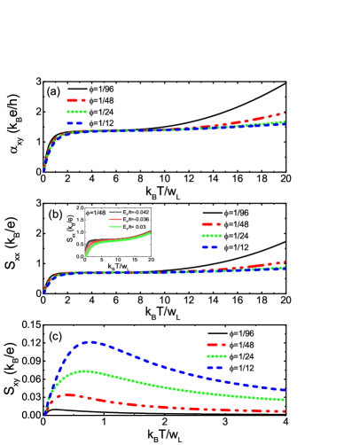
Figure 4: (color online). The temperature dependence of (a) $\alpha_{xy}$, (b) $S_{xx}$, and (c) $S_{xy}$ at central LL for different magnetic flux $\phi=1/96$, $1/48$, $1/24$, and $1/12$, respectively. The inset of (b) shows the temperature dependence of $S_{xx}$ for certain fixed Fermi energies. The system size is chosen as $N=192\times 4\times 8$, the disorder strength is set to $W/t=0.2$.

III.2 Thermoelectric transport

Now we turn to the disorder effect on the thermoelectric transport coefficients in the presence of the strong magnetic field supplement . In Fig. 3, we first plot the calculated thermoelectric conductivities at some finite temperatures. Here, the temperature dependence is shown as a function of the ratio between $k_{B}T$ and $W_{L}$, where $W_{L}$ represents the full-width at the half-maximum of the longitudinal conductivity $\sigma_{xx}$ peaks around zero energy. As shown in Figs. 3(a)-(b), the transverse thermoelectric conductivity $\alpha_{xy}$ displays a series of peaks, while the longitudinal thermoelectric conductivity ${\alpha_{xx}}$ undergoes a sign reversal and approaches zero at the center of each LL. In Fig. 3(c), we show $\alpha_{xy}$ as a function of the temperature for different Fermi energies. At low-temperature region, $k_{B}T\ll W_{L}$, $\alpha_{xy}$ increases quickly. When $k_{B}T$ becomes comparable to or greater than $W_{L}$, $\alpha_{xy}$ for all Fermi energies reaches a constant value $1.38k_{B}e/h$, which matches exactly the universal value $g(\ln 2)k_{B}e/h$ predicted for 2D QHE systems Jonson1984 ; UnivJPC1984 , with degeneracy $g=2$. This robust flat plateau feature demonstrates the LL quantization (only states within the degenerating LLs contribute to the $\alpha_{xy}$), which can be probed in experimental measurements at low temperatures. However, in the high-temperature region, when $k_{B}T\gg W_{L}$, the value of $\alpha_{xy}$ continues to rise with increasing temperature without saturation. This non-saturating property at higher temperatures survives even when the quantized Hall plateaus disappear with $n_{z}\rightarrow\infty$ Fu2019 ; Skinner2018 . Furthermore, we show quantitative behavior of the ratio of the $\alpha_{xy}$ versus the normalized temperature $k_{B}T/W_{L}$ in the inset of Figs. 3(c). As we can see, $\alpha_{xy}/(k_{B}T/W_{L})$ curves collapse into a constant plateau at high temperature.

We further demonstrate some interesting features of thermoelectric coefficients for different magnetic field strengths. As seen from Fig. 4(a), we first plot $\alpha_{xy}$ as a function of the normalized temperature $k_{B}T/W_{L}$ with increasing magnetic field strength from $\phi=1/96$ to $\phi=1/12$. At relatively low temperature regions, all the curves of $\alpha_{xy}$ approach a constant value about $1.38k_{B}e/h$. With increasing temperature, $\alpha_{xy}$ for different magnetic field strengths all increase gradually. Interestingly, the weaker the magnetic field strength is, the faster $\alpha_{xy}$ grows. In Figs. 4(b) and (c), we show the temperature dependence of the thermopower $S_{xx}$ and Nernst signal $S_{xy}$ supplement , which can be directly measured in experiments Ong2017 . At relatively high-temperature region, we also observe the values of $S_{xx}$ increase quickly with the decrease of the magnetic field strength, and the values are inversely proportional to $B$. The inset of Fig. 4(b) shows the temperature dependence of $S_{xx}$ for some different Fermi energies. With increasing temperature, the peak values from Fermi energies continue to grow gradually with temperature without saturation. We suggest that these striking features can be attributed to the thermal excitations between different $n=0$ LLs. In Fig. 4(c), $S_{xy}$ assumes the Arrhenius form $(1/T)e^{-E_{F}/k_{B}T}$ with the increase of temperature. The peak values are also proportional to the magnetic field strength, i.e., $S_{xy}\propto B$. When the magnetic field strength increases from $\phi=1/96$ to $\phi=1/12$, the peak value of $S_{xy}$ reaches $0.12$ $k_{B}/e$ ($10.35$ $\mu V/K$), which is in agreement with the minimum measured value $\sim 8$ $\mu V/K$ Caglieris2018 . More interestingly, in these curves $S_{xy}$ shows a broadened maximum around $k_{B}T=0.5W_{L}$ for strong magnetic fields $B$, which shifts to a lower temperature by decreasing $B$. This similar maximum has also been observed in the experiments for the compound TaP and NbP Caglieris2018 ; Watzman2018 .

IV Summary

In summary, we numerically investigate the 3D QHE and thermoelectric transport properties of Weyl semimetals in the presence of disorder. When a perpendicular magnetic field is applied, we observe well-formed Hall plateaus in units of $e^{2}/h$ for an intermediate number of layers and a finite range of Fermi energy near the Weyl points. We demonstrate how the system size, magnetic field strength and disorder influence the quantized Hall plateaus. Both $\alpha_{xy}$ and $S_{xx}$ exhibit non-saturating characteristic features with increasing temperature, which are robust in the thermodynamic limit. However, for lower temperatures, $\alpha_{xy}$ for all Fermi energies reaches a constant plateau value 1.38$k_{B}e/h$, signaling the LL quantization. Our work provides a clearer understanding of the topological 3D QHE and magnetothermoelectric transport in Weyl semimetals.

APPENDIX

Following the Eq.(2) in the main text, we exactly diagonalize the model Hamiltonian in the presence of disorder Sheng1997 , and obtain the transport coefficients by using the energy spectra and wave functions. In practice, we can first calculate the electrical conductivities $\sigma_{ij}$ at zero temperature, and then use the relation Jonson1984 ; UnivJPC1984

$$\sigma_{ij}(E_{F},T) = \int d\epsilon\,\sigma_{ij}(\epsilon)\left(-{\partial f(\epsilon)\over\partial\epsilon}\right),$$ (4)

$$\alpha_{ij}(E_{F},T) = {-1\over eT}\int d\epsilon\,\sigma_{ij}(\epsilon)(\epsilon-E_{F})\left(-{\partial f(\epsilon)\over\partial\epsilon}\right),$$ (5)

to obtain the electrical and thermoelectric conductivities at finite temperatures. The thermopower and Nernst signal can be calculated subsequently from Ong2017 ; footnote1

$$-S_{xx} = {E_{x}/\mid\nabla T\mid}=-({\rho_{xx}\alpha_{xx}-\rho_{xy}\alpha_{xy}}),$$ (6)

$$S_{xy} = {E_{y}/\mid\nabla T\mid}=({\rho_{xx}\alpha_{xy}+\rho_{xy}\alpha_{xx}}),$$ (7)

where $\rho_{ij}$ is the resistivity tensor.

References

- (1) X. Wan, A. M. Turner, A. Vishwanath and S. Y. Savrasov, Phys. Rev. B 83, 205101 (2011).
- (2) H. Weng, C. Fang, Z. Fang, B. A. Bernevig, and X. Dai, Phys. Rev. X 5, 011029 (2015).
- (3) Q. D. Jiang, H. Jiang, H. Liu, Q. F. Sun, and X. C. Xie, Phys. Rev. Lett. 115, 156602 (2015).
- (4) C. Z. Chen, J. Song, H. Jiang, Q. F. Sun, Z. Wang, and X. C. Xie, Phys. Rev. Lett. 115, 246603 (2015).
- (5) S. M. Huang, S. Y. Xu, I. Belopolski, C. C. Lee, G. Chang, B. Wang, N. Alidoust, G. Bian, M. Neupane, A. Bansil, H. Lin and M. Z. Hasan, Nat. Commun. 6, 7373 (2015).
- (6) L. X. Yang, Z. K. Liu, Y. Sun, H. Peng, H. F. Yang, T. Zhang, B. Zhou, Y. Zhang, Y. F. Guo, M. Rahn, D. Prabhakaran, Z. Hussain, S. K. Mo, C. Felser, B. Yan, Y. L. Chen, Nat. Phys. 11, 728 (2015).
- (7) S. Y. Xu, I. Belopolski, N. Alidoust, M. Neupane, G. Bian, C. Zhang, R. Sankar, G. Chang, Z. Yuan, C. C. Lee, S. M. Huang, H. Zheng, J. Ma, D. S. Sanchez, B. Wang, A. Bansil, F. Chou, P. P. Shibayev, H. Lin, S. Jia, and M. Z. Hasan, Science 349, 613 (2015).
- (8) B. Q. Lv, H. M. Weng, B. B. Fu, X. P. Wang, H. Miao, J. Ma, P. Richard, X. C. Huang, L. X. Zhao, G. F. Chen, Z. Fang, X. Dai, T. Qian, and H. Ding, Phys. Rev. X 5, 031013 (2015).
- (9) B. Q. Lv, N. Xu, H. M. Weng, J. Z. Ma, P. Richard, X. C. Huang, L. X. Zhao, G. F. Chen, C. Matt, F. Bisti, V. Strokov, J. Mesot, Z. Fang, X. Dai, T. Qian, M. Shi, H. Ding, Nat. Phys. 11, 724 (2015).
- (10) H. B. Nielsen and M. Ninomiya, Phys. Lett. B 130, 389 (1983).
- (11) Kai-Yu Yang, Yuan-Ming Lu, and Ying Ran, Phys. Rev. B 84, 075129 (2011).
- (12) M. M. Vazifeh and M. Franz, Phys. Rev. Lett. 111, 027201 (2013).
- (13) S. A. Parameswaran, T. Grover, D. A. Abanin, D. A. Pesin, and A. Vishwanath, Phys. Rev. X 4, 031035 (2014).
- (14) D. T. Son and B. Z. Spivak, Phys. Rev. B 88, 104412 (2013).
- (15) A. A. Burkov, Phys. Rev. Lett. 113, 247203 (2014).
- (16) Hai-Zhou Lu, Song-Bo Zhang, and Shun-Qing Shen, Phys. Rev. B 92, 045203 (2015).
- (17) S. Nandy, G. Sharma, A. Taraphder, and S. Tewari, Phys. Rev. Lett. 119, 176804 (2017).
- (18) A. A. Burkov, Phys. Rev. B 96, 041110(R) (2017).
- (19) N. Kumar, S. N. Guin, C. Felser, and C. Shekhar, Phys. Rev. B 98, 041103(R) (2018).
- (20) J. Yang, W. L. Zhen, D. D. Liang, Y. J. Wang, X. Yan, S. R. Weng, J. R. Wang, W. Tong, L. Pi, W. K. Zhu, and C. J. Zhang, Phys. Rev. Mater. 3, 014201 (2019).
- (21) C. M. Wang, Hai-Peng Sun, Hai-Zhou Lu and X. C. Xie, Phys. Rev. Lett. 119, 136806 (2017).
- (22) Hai-Zhou Lu, National Science Review 6, 208 (2019).
- (23) Hai-Peng Sun and Hai-Zhou Lu, Frontiers of Physics 14, 33405 (2019).
- (24) Cheng Zhang, Awadhesh Narayan, Shiheng Lu, Jinglei Zhang, Huiqin Zhang, Zhuoliang Ni, Xiang Yuan, Yanwen Liu, Ju-Hyun Park, Enze Zhang, Weiyi Wang, Shanshan Liu, Long Cheng, Li Pi, Zhigao Sheng, Stefano Sanvito and Faxian Xiu, Nat. Commun. 8, 1272 (2017).
- (25) Cheng Zhang, Yi Zhang, Xiang Yuan, Shiheng Lu, Jinglei Zhang, Awadhesh Narayan, Yanwen Liu, Huiqin Zhang, Zhuoliang Ni, Ran Liu, Eun Sang Choi, Alexey Suslov, Stefano Sanvito, Li Pi, Hai-Zhou Lu, Andrew C. Potter and Faxian Xiu, Nature 565, 331 (2019).
- (26) Ben-Chuan Lin, Shuo Wang, Steffen Wiedmann, Jian-Ming Lu, Wen-Zhuang Zheng, Dapeng Yu and Zhi-Min Liao, Phys. Rev. Lett. 122, 036602 (2019).
- (27) Masaki Uchida, Yusuke Nakazawa, Shinichi Nishihaya, Kazuto Akiba, Markus Kriener, Yusuke Kozuka, Atsushi Miyake, Yasujiro Taguchi, Masashi Tokunaga, Naoto Nagaosa, Yoshinori Tokura and Masashi Kawasaki, Nat. Commun. 8, 2274 (2017).
- (28) Zhi-Peng Gao, Zhi Li, Dan-Wei Zhang, Physics Letters A 382, 3205 (2018).
- (29) Hailong Li, Haiwen Liu, Hua Jiang and X. C. Xie, Phys. Rev. Lett. 125, 036602 (2020).
- (30) Fangdong Tang, Yafei Ren, Peipei Wang, Ruidan Zhong, John Schneeloch, Shengyuan A. Yang, Kun Yang, Patrick A. Lee, Genda Gu, Zhenhua Qiao and Liyuan Zhang, Nature 569, 537 (2019).
- (31) Fang Qin, Shuai Li, Z. Z. Du, C. M. Wang, Hai-Zhou Lu and X. C. Xie, Phys. Rev. Lett. 125, 206601 (2020).
- (32) Z. Jia, C. Li, X. Li, J. Shi, Z. Liao, D. Yu and X. Wu, Nat. Commun. 7, 13013 (2016).
- (33) F. Caglieris, C. Wuttke, S. Sykora, V. Süss, C. Shekhar, C. Felser, B. Büchner, and C. Hess, Phys. Rev. B 98, 201107(R) (2018).
- (34) S. J. Watzman, T. M. McCormick, C. Shekhar, S. C. Wu, Y. Sun, A. Prakash, C. Felser, N. Trivedi, and J. P. Heremans, Phys. Rev. B 97, 161404 (2018).
- (35) M. Hirschberger, S. Kushwaha, Z. Wang, Q. Gibson, S. Liang, C. A. Belvin, B. A. Bernevig, R. J. Cava, and N. P. Ong, Nature Materials 15, 1161 (2016).
- (36) F. C. Chen, H. Y. Lv, X. Luo, W. J. Lu, Q. L. Pei, G. T. Lin, Y. Y. Han, X. B. Zhu, W. H. Song, and Y. P. Sun, Phys. Rev. B 94, 235154 (2016).
- (37) J. Gooth, A. C. Niemann, T. Meng, A. G. Grushin, K. Landsteiner, B. Gotsmann, F. Menges, M. Schmidt, C. Shekhar, V. Sü, R. Hühne, B. Rellinghaus, C. Felser, B. Yan, and K. Nielsch, Nature 547, 324 (2017).
- (38) G. Sharma, P. Goswami, and S. Tewari, Phys. Rev. B 93, 035116 (2016).
- (39) Haiyang Yang, Wei You, Jialu Wang, Junwu Huang, Chuanying Xi, Chao Cao, Mingliang Tian, Zhu-An Xu, Jianhui Dai, and Yuke Li, Phys. Rev. Materials 4, 024202 (2020).
- (40) E. V. Gorbar, V. A. Miransky, I. A. Shovkovy, and P. O. Sukhachov, Phys. Rev. B 96, 155138 (2017).
- (41) Vladyslav Kozii, Brian Skinner, and Liang Fu, Phys. Rev. B 99, 155123 (2019).
- (42) B. Skinner and L. Fu, Science Advances 4, 2621 (2018).
- (43) Fei Han, Nina Andrejevic, Thanh Nguyen, Vladyslav Kozii, Quynh Nguyen, Zhiwei Ding, Ricardo Pablo-Pedro, Shreya Parjan, Brian Skinner, Ahmet Alatas, Ercan Alp, Songxue Chi, Jaime Fernandez-Baca, Shengxi Huang, Liang Fu, and Mingda Li, Nat. Commun. 11, 6167 (2020).
- (44) N. P. Armitage, E. J. Mele, and A. Vishwanath, Rev. Mod. Phys. 90, 015001 (2018).
- (45) Y. Huo and R. N. Bhatt, Phys. Rev. Lett. 68, 1375 (1992).
- (46) D. N. Sheng and Z. Y. Weng, Phys. Rev. Lett. 78, 318 (1997).
- (47) Ming-Xun Deng, G. Y. Qi, R. Ma, R. Shen, Rui-Qiang Wang, L. Sheng and D. Y. Xing, Phys. Rev. Lett. 119, 036601 (2019).
- (48) W. Zhu, Q. W. Shi, X. R. Wang, J. Chen, J. L. Yang, and J. G. Hou, Phys. Rev. Lett. 102, 056803 (2009).
- (49) M. Jonson and S. M. Girvin, Phys. Rev. B 29, 1939 (1984).
- (50) Z. G. Chen, R. Y. Chen, R. D. Zhong, J. Schneeloch, C. Zhang, Y. Huang, F. Qu, R. Yu, Q. Li, G. D. Gu, and N. L. Wang, PNAS 114, 816 (2017).
- (51) C. Shekhar, A. K. Nayak, Y. Sun, M. Schmidt, M. Nicklas, I. Leermakers, U. Zeitler, Y. Skourski, J. Wosnitza, Z. Liu, Y. Chen, W. Schnelle, H. Borrmann, Y. Grin, C. Felser, and B. Yan, Nature Phys. 11, 645 (2015).
- (52) See Supplemental Material at [URL will be inserted by publisher] for a discussion about the thermopower and Nernst signal as functions of Fermi energy at four different temperatures.
- (53) H. Oji, J. Phys. C 17, 3059 (1984).
- (54) Tian Liang, Jingjing Lin, Quinn Gibson, Tong Gao, Max Hirschberger, Minhao Liu, R. J. Cava, and N. P. Ong, Phys. Rev. Lett. 118, 136601 (2017).
- (55) Different literatures may have a sign difference due to different conventions.