A Neural-Network Variational Quantum Algorithm for Many-Body Dynamics

Abstract

We propose a neural-network variational quantum algorithm to simulate the time evolution of quantum many-body systems. Based on a modified restricted Boltzmann machine (RBM) wavefunction ansatz, the proposed algorithm can be efficiently implemented in near-term quantum computers with low measurement cost. Using a qubit recycling strategy, only one ancilla qubit is required to represent all the hidden spins in an RBM architecture. The variational algorithm is extended to open quantum systems by employing a stochastic Schrödinger equation approach. Numerical simulations of spin-lattice models demonstrate that our algorithm is capable of capturing the dynamics of closed and open quantum many-body systems with high accuracy without suffering from the vanishing gradient (or ‘barren plateau’) issue for the considered system sizes.

I Introduction

Accurate and efficient simulation of quantum many-body dynamics remains one of the most challenging problems in physics, despite nearly a century of progress. Renewed interest has been sparked in this field due to recent experiments with Rydberg atomsBernien et al. (2017); Celi et al. (2020), which suggest the existence of scar states which do not thermalize. This has lead to new studies of fragmented Hilbert spaces for such constrained modelsSala et al. (2020); Yang et al. (2020); De Tomasi et al. (2019), along with further studies on fractons, which are restricted excitations which can disperse only in certain directionsNandkishore and Hermele (2019); Chamon (2005). These studies also tie in to the more established field of many body localizationAlet and Laflorencie (2018); Pal and Huse (2010); Nandkishore and Huse (2015), which studies the possibility of extremely slow relaxation of high energy states in systems with strong disorder. As many of the above phenomena are hard to study analytically, there is a strong motivation to develop powerful numerical tools to further our understanding.

One of the most powerful numerical tools at the disposal of condensed matter theorists is quantum Monte Carlo, which has performed remarkably well for equilibrium physics of numerous systemsSuzuki (1993); Ceperley and Alder (1986). This has made important the applicability of this technique to study real time dynamics. This is often impossible due to the infamous sign problemBishop and Farnell (2000); Troyer and Wiese (2005), and one of the few promising ways in which practitioners have attempted to avoid this is by transferring the real time behavior to functions which form coefficients in the wavefunction. These functions then need to have a variational form which can be optimised to get reasonably good results on small systemsCarleo et al. (2017); Ido et al. (2015). Even though one can get around the sign problem for these cases, severe ergodicity restrictions in the Monte Carlo updates may render them inefficient, and necessitate specialized algorithmsBiswas et al. (2016); Syljuåsen and Sandvik (2002); Yan et al. (2019). To allow variational wavefunctions a higher degree of expressibility, some ideas from machine learning, such as restricted Boltzmann machines (RBM), have been usedCarleo and Troyer (2017); Nagy and Savona (2019); Glasser et al. (2018); Schmitt and Heyl (2019); Gutiérrez and Mendl (2019); Deng et al. (2017); Sarma et al. (2019) to serve as a representation. This has lead to a well-controlled way of approximating complicated wavefunctions with rich spatial features. Neural networks have also been used to simulate open quantum systems, which are numerically more challenging to study than closed systems, and promising results have been achieved for both dynamicalHartmann and Carleo (2019) and steady stateNagy and Savona (2019); Vicentini et al. (2019); Yoshioka and Hamazaki (2019) features.

Due to recent advances in quantum computing, it has become possible to program a small number of qubits to directly represent a quantum system using Noisy Intermediate-Scale Quantum (NISQ) technologyPreskill (2018); Arute et al. (2019). One of the many applications of this set up is to speed up the optimization step for variational wavefunctionsMcClean et al. (2016); Peruzzo et al. (2014); Farhi et al. (2014); Kandala et al. (2017); Hempel et al. (2018); Colless et al. (2018). This serves as a substantial improvement for cases where variational Monte Carlo is inefficient. Direct variational optimization of the time-dependent Schrödinger equationLi and Benjamin (2017); Yuan et al. (2019); Heya et al. (2019); Lee et al. (2021) has also shown promise, and a large number of general processes can be mapped on to this techniqueEndo et al. (2020).

In this work, we engineer a neural-network variational quantum algorithm to simulate the dynamics of quantum many-body systems. The algorithm integrates the power of an RBM representation of quantum states with a quantum speed-up coming from transferring the computationally heavy step of calculating expectation values on to the quantum computer. We show that the variational algorithm can be extended to the dynamics of open quantum systems using a stochastic Schrödinger equation approach. The proposed method is benchmarked against canonical spin-lattice models and performs well for dynamics of both closed and open systems.

II Neural Network Quantum States

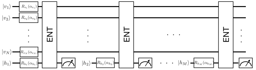
Figure 1: Quantum circuit for preparing uRBM state with qubit recycling scheme described in Eq. 4. All the qubits are initialized in $|0\rangle$ state. The single rotations are governed by the relations in Eq. 5. The $j$-th entangling block implements the $\exp(\mathrm{i}\sum_{i}W_{ij}^{I}\hat{v}^{z}_{i}\hat{h}^{z}_{j})$ operator and its explicit form is given in the Appendix A. After each entangling block, the ancilla qubit representing the $j$-th hidden spin is projected onto $|+\rangle$ state before being recycled.

An RBM quantum state can be obtained from a bipartite Ising Hamiltonian

$$\hat{H}_{RBM}(\theta)=\sum_{i}b_{i}\hat{v}^{z}_{i}+\sum_{j}m_{j}\hat{h}^{z}_{j}+\sum_{ij}W_{ij}\hat{v}^{z}_{i}\hat{h}^{z}_{j},$$ (1)

where $\hat{v}^{z}_{i}$ or $\hat{h}^{z}_{j}$ is the Pauli-Z operator for the visible or hidden qubit, respectively. We denote the complex-valued variational RBM parameters as $\theta=[b,m,W]$. To prepare a complex-valued RBM state using a state preparation protocol proposed in Ref. Hsieh et al. (2021), we first entangle $N+M$ qubits (representing $N$ visible and $M$ hidden spins of an RBM architecture) according to

$$|\Psi_{vh}(\theta)\rangle = \frac{e^{\hat{H}_{RBM}(\theta)}}{N_{vh}}|++\dots+\rangle_{vh},$$ (2)

where $|+\rangle=\frac{1}{\sqrt{2}}(|0\rangle+|1\rangle)$, $N_{vh}=\sqrt{\prescript{}{vh}{\langle++\dots+|}e^{2\hat{H}^{R}_{RBM}(\theta)}|++\dots+\rangle_{vh}}$, $\hat{H}^{R}_{RBM}(\theta)$ is the Hermitian part of the RBM Hamiltonian and the subscript $vh$ denotes visible and hidden (ancilla) qubits. Eq. 2 gives a conceptually simple wave function that could be generated by first applying single-qubit transformations $\exp(b_{i}\hat{v}^{z}_{i})$ and $\exp(m_{j}\hat{h}^{z}_{j})$ on individual qubits followed by $\exp(W_{ij}\hat{v}^{z}_{i}\hat{h}^{z}_{j})$ to couple the visible and hidden qubits.

Once the extended wave function $|\Psi_{vh}(\theta)\rangle$ is generated, all ancilla qubits (i.e. hidden spins) are post-selected for $|+\rangle_{h}$ and the desired RBM state is implemented in a quantum circuit

$$|\Psi_{v}(\theta)\rangle = \frac{\prescript{}{h}{\left\langle++\dots+|\Psi_{vh}(\theta)\right\rangle}}{N_{v}},$$ (3)

where $N_{v}=\sqrt{\langle\Psi_{vh}(\theta)|\hat{P}^{(h)}_{+}|\Psi_{vh}(\theta)\rangle}$ and $\hat{P}_{+}^{(h)}=|++\dots+\rangle_{h}\langle++\dots+|$ projects all the hidden spins onto $|+\rangle$ state.

Observing that Eq. 3 can be cast in the following form:

$$|\Psi_{v}(\theta)\rangle=\frac{1}{N_{v}}\left[\prescript{}{}{\langle+|}\left[e^{\hat{h}^{z}_{M}\left(m_{M}+\sum_{i}W_{iM}\hat{v}^{z}_{i}\right)}\right]|+\rangle\right]_{M}$$ (4)

$$\times\left[\prescript{}{}{\langle+|}\left[e^{\hat{h}^{z}_{M-1}\left(m_{M-1}+\sum_{i}W_{iM-1}\hat{v}^{z}_{i}\right)}\right]|+\rangle\right]_{M-1}\cdots$$

$$\left[\prescript{}{}{\langle+|}\left[e^{\hat{h}^{z}_{1}\left(m_{1}+\sum_{i}W_{i1}\hat{v}^{z}_{i}\right)}\right]|+\rangle\right]_{1}\,\,e^{\sum_{i}b_{i}\hat{v}^{z}_{i}}|++\cdots+\rangle_{v},$$

where $[\langle+|[...]|+\rangle]_{j}$ encodes the effect of $j$-th hidden spin on all visible spins, it is clear that a single ancilla qubit is sufficient to implement the entangling operation sequentially.

The above quantum operations are non-unitary when RBM parameters are complex, i.e. $b_{i}^{R}\neq 0$, $m_{j}^{R}\neq 0$ or $W^{R}_{ij}\neq 0$, where we use superscripts $R$ and $I$ to denote the real and imaginary parts of the RBM parameters. In particular, the non-unitary two-qubit operations mediating entanglement across the visible-hidden layer are difficult to implement. One could adopt a probabilistic scheme Xia and Kais (2018) to generate the inter-layer couplings with an extra ancilla qubit. However this approach is difficult to scale with the number of qubits since it involves $N*M$ projective measurements. The probability of one successful sampling has therefore a lower bound of $\mbox{e}^{-2\sum_{ij}|w_{ij}|}\sim\mbox{e}^{-O(NM)}$.

For this reason, we only consider the unitary-coupled RBM (uRBM) ansatz in which $W^{R}_{ij}=0$ for the rest of this letter Hsieh et al. (2021). Fig. 1 depicts a quantum circuit for preparing a uRBM state composed of $N$ visible spins and $M$ hidden spins. After initializing all qubits in $|0\rangle$ state, we first perform single qubit rotations representing the terms $\exp(b_{i}\hat{v}_{i}^{z})$ and $\exp(m_{j}\hat{h}_{j}^{z})$. The rotation angles, $\alpha_{v_{i}/h_{j}}$, are governed by the relations

$$R_{v_{i}}(\alpha_{v_{i}})|0\rangle = \text{e}^{b_{i}\hat{v}_{i}^{z}}|+\rangle/c_{v_{i}},$$ (5)

$$R_{h_{j}}(\alpha_{h_{j}})|0\rangle = \text{e}^{m_{j}\hat{h}_{j}^{z}}|+\rangle/c_{h_{j}},$$

where the normalization factors are $c_{v_{i}}=\sqrt{\langle+|\exp\left(2b_{i}^{R}\hat{v}^{z}_{i}\right)|+\rangle}$ and $c_{h_{j}}=\sqrt{\langle+|\exp\left(2m_{j}^{R}\hat{h}^{z}_{j}\right)|+\rangle}$. The $j$-th entangling block implements the coupling $\exp(\mathrm{i}\sum_{i}W_{ij}^{I}\hat{v}^{z}_{i}\hat{h}^{z}_{j})$ and are composed of a series of controlled-Z rotations (see Appendix A for details). Employing the qubit recycling scheme described in Eq. 4, the ancilla qubit representing the $j$-th hidden spin is projected onto $|+\rangle$ state after each entangling block before being recycled. Thus we only need $N+1$ qubits in total, and the number of quantum gates is proportional to the number of variational parameters, $N_{var}$, which scales as $O(\alpha N^{2})$ where $\alpha=M/N$.

With uRBM, there are only $M$ projective measurements of hidden spins on $|+\rangle$ state, therefore the success probability has improved to $\mbox{e}^{-O(M)}$. We can further mitigate these probabilistic projective measurements. One approach is to re-scale the variational parameters such that the hidden spins remain close to the $|+\rangle$ state (see Ref. Xia and Kais (2018)). Alternatively, we can use a Monte Carlo scheme with classical post-processing (see Appendix B) that enables us to entirely circumvent the post-selection.

III Time-dependent Variational Algorithm

We adopt a hybrid quantum-classical approach based on the time-dependent variational Monte Carlo (t-VMC) method to simulate the quantum dynamics Carleo et al. (2012, 2014); Becca and Sorella (2017). In the t-VMC framework, we minimize the residue in $\text{min}_{\theta}||\mathrm{i}\frac{\partial|\Psi(\theta)\rangle}{\partial t}-\hat{H}_{s}|\Psi(\theta)\rangle||,$ where $\hat{H}_{s}$ is the system Hamiltonian and the norm is defined as the square root of the inner product. The resulting equations of motion for the time-dependent variational parameters are

$$\dot{\theta}_{n}=\sum_{m}A_{nm}^{-1}\,\text{Im}[f_{m}].$$ (6)

The covariance matrix $A$ and force vector $f$ read

$$A_{nm} = \text{Re}\langle\hat{O}^{\dagger}_{n}\hat{O}_{m}\rangle_{v}-\text{Re}\langle\hat{O}^{\dagger}_{n}\rangle_{v}\text{Re}\langle\hat{O}_{m}\rangle_{v},$$ (7)

$$f_{m} = \langle\hat{O}^{\dagger}_{m}\hat{H}_{s}\rangle_{v}-\text{Re}\langle\hat{O}^{\dagger}_{m}\rangle_{v}\langle\hat{H}_{s}\rangle_{v},$$ (8)

where $\langle\cdots\rangle_{v}=\langle\Psi_{v}(\theta)|\,\cdots\,|\Psi_{v}(\theta)\rangle$. The derivative operators with respect to the $n$-th variational parameter is defined as $\hat{O}_{n}=\frac{\partial\ln{|\Psi_{v}(\theta)\rangle}}{\partial\theta_{n}}$. For RBM state defined in Eq. 3, the $\hat{O}_{n}$ operators can be derived analytically which allows an efficient way of obtaining the gradients

$$\hat{O}_{n}=\left\{\begin{array}[]{ll}\mathrm{i}^{1-\delta}\hat{v}^{z}_{i},&\text{ if }\theta_{n}=b_{i},\\ \mathrm{i}^{1-\delta}\tanh\left(m_{j}+\sum_{i}W_{ij}\hat{v}^{z}_{i}\right),&\text{ if }\theta_{n}=m_{j},\\ \mathrm{i}\hat{v}^{z}_{i}\tanh\left(m_{j}+\sum_{i}W_{ij}\hat{v}^{z}_{i}\right),&\text{ if }\theta_{n}=W_{ij},\\ \end{array}\right.$$ (12)

where $\delta=0$ if $\theta_{n}=b^{I}_{i}$ or $\theta_{n}=m^{I}_{j}$ or $\theta_{n}=W^{I}_{i}$, and $\delta=1$ if $\theta_{n}=b^{R}_{i}$ or $\theta_{n}=m^{R}_{j}$. The variational parameters are updated iteratively according to $\theta_{n}(t+\delta t)=\theta_{n}(t)+\sum_{m}A_{nm}^{-1}\,\text{Im}[f_{m}]\delta t$ where $\delta t$ is the update time step.

In conventional t-VMC, the covariance matrix $A$ and force vector $f$ in Eq. 7 are obtained from Markov chain random walk approach, such as the Metropolis-Hastings algorithm. Such sampling could be challenging for systems that exhibit long correlation time, e.g. systems near phase transition. In a hybrid quantum-classical framework, both $A$ and $f$ are sampled directly from the output of quantum circuit depicted in Fig. 1, circumventing the difficulties associated with Markov chain methods.

IV Simulation Results

To demonstrate the performance of the uRBM algorithm in simulating many-body quantum dynamics, we first consider a 1D transverse-field Ising (TFI) model:

$$\hat{H}_{TFI} = -h\sum_{i}\hat{\sigma}_{i}^{x}-\sum_{<ij>}\hat{\sigma}_{i}^{z}\hat{\sigma}_{j}^{z},$$ (13)

where $h$ denotes the strength of the transverse field. Here we study the dynamics of a TFI model induced by quantum quench. The TFI system is initially prepared in the ground state for an initial transverse field $h_{i}$. The variational parameters of the initial ground state wavefunction are obtained using a hybrid imaginary time algorithm (see Appendix C). At $t=0$, we introduce an instantaneous change to the transverse field, $h_{f}\neq h_{i}$, and let the system evolve under the new Hamiltonian.

In Fig. 2 (a) and (b), we consider a TFI model of 14 spins with periodic boundary condition and the transverse field is changed from $h_{i}=0.5$ to the critical value of $h_{f}=1.0$ at $t=0$. In the simulations we use $\delta t=0.0005$ and $\alpha=M/N=8$. We compare the results from the uRBM algorithm with results from exact diagonalization by studying the evolution of transverse spin polarization $\langle\sigma_{1}^{x}\rangle$ and its correlation $\langle\sigma_{1}^{x}\sigma_{2}^{x}\rangle$. The good agreement with exact results confirms the accuracy of the uRBM algorithm in capturing quantum many-body dynamics.

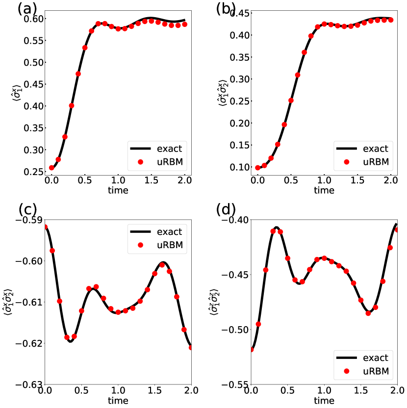
Figure 2: Time evolution induced by quantum quench. Results from uRBM algorithm (symbols) are compared to exact calculations (solids lines). (a) and (b) Dynamics of transverse polarization and its correlation in a 1D Ising model. (c) and (d) Dynamics of magnetization and transverse polarization correlations in a 1D Heisenberg model in a global field.

Next we consider a 1D anisotropic Heisenberg model with periodic boundary condition in a magnetic field:

$$\hat{H}_{H} = -h_{z}\sum_{i}\hat{\sigma}_{i}^{z}+\sum_{<ij>}(J_{z}\hat{\sigma}_{i}^{z}\hat{\sigma}_{j}^{z}+\hat{\sigma}_{i}^{x}\hat{\sigma}_{j}^{x}+\hat{\sigma}_{i}^{y}\hat{\sigma}_{j}^{y}),$$ (14)

where $h_{z}$ is the strength of longitudinal field and $J_{z}$ is the longitudinal coupling. We perform a quantum quench by instantaneously changing the longitudinal coupling from $J_{z}=1.0$ to $J_{z}=0.5$ at $t=0$. Figs. 2 (c) and (d) depict the dynamics of spin-spin correlations of a 14-spin Heisenberg model with $h_{z}=1.0$. We use $\delta t=0.0002$ and $\alpha=8$ in our simulations. Again we observe near exact agreement between the results from the uRBM algorithm and exact diagonalization, further confirming the capability of the hybrid uRBM algorithm. This can easily be generalized to the more interesting case of random fields in the $z$-direction, which allows the integrable Heisenberg chain to express chaotic behavior and many-body localization Luitz et al. (2015). Additionally, we also perform the uRBM simulation of a two dimensional triangular anti-ferromagnetic Ising model (see Appendix D), and again observe excellent agreement with exact calculations.

V Open Quantum Systems

Extending the variational uRBM algorithm to open quantum systems is conceptually straight forward using the stochastic wavefunction approach. The dynamics of the density matrix, $\hat{\rho}$, of an open quantum system can be described by the Linblad master equation Breuer and Petruccione (2007)

$$\frac{d\hat{\rho}}{dt}=-\mathrm{i}[\hat{H}_{s},\hat{\rho}]+\frac{1}{2}\sum_{k}[2\hat{L}_{k}\hat{\rho}\hat{L}_{k}^{\dagger}-\{\hat{L}_{k}^{\dagger}\hat{L}_{k},\hat{\rho}\}],$$ (15)

where $\{.\}$ denotes an anti-commutator, $\hat{H}_{s}$ is the system Hamiltonian and the Linblad operators $\hat{L}_{k}$ describe the interaction between the system and a Markovian bath. Instead of solving the Linblad master equation directly, an open quantum system can be equivalently described by an ensemble of pure state trajectories Dalibard et al. (1992); Carmichael (1993). The evolution of these pure state trajectories is governed by a non-Hermitian effective Hamiltonian $\hat{H}_{eff}=\hat{H}_{s}-\frac{\mathrm{i}}{2}\sum_{k}(\hat{L}_{k}\hat{L}_{k}^{\dagger}-\langle\hat{L}_{k}\hat{L}_{k}^{\dagger}\rangle)$ and subject to continuous measurement. The details of implementing these stochastic wavefunction trajectories in quantum circuits can be found in Appendix J.

We test the ability of the hybrid uRBM algorithm in simulating the dynamics of an open quantum system by considering a 6-spin 1D TFI model with open boundary condition coupled to a Markovian bath. All the spins of the TFI model are initially prepared in $|+\rangle=\frac{1}{\sqrt{2}}(|0\rangle+|1\rangle)$ state. The Linblad operator is $\hat{L}_{k}=\sqrt{\gamma}\hat{\sigma}_{k}^{+}$ where $\hat{\sigma}_{k}^{+}$ is a raising operator acting on the $k$-th spin and $\gamma$ determines the strength of system-bath interaction. Other parameters used in the simulation are $\alpha=M/N=6$, $\gamma=0.05$, $h=1.0$, $\delta t=0.0005$. The dynamics of transverse polarization and its correlation are compared to those from directly solving Eq. 15. It can be seen that the uRBM algorithm is capable of simulating the dynamics of open systems with high accuracy. This further extends the applicability of the hybrid uRBM algorithm to study novel non-equilibrium phenomena in many-body open quantum systems such as phase transitions Fink et al. (2018); Raftery et al. (2014).

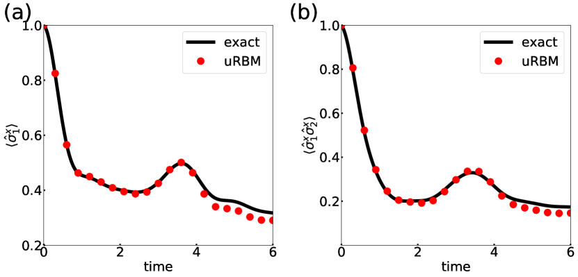
Figure 3: Dynamics of a dissipative 1D Ising model obtained from exact numerical solution of Eq.15 (solid lines) and from the hybrid uRBM algorithm (symbols). The simulation results from the hybrid uRBM algorithm are obtained from averaging over 10000 pure state trajectories, and the error bars are smaller than the symbols

VI Discussions

The proposed hybrid uRBM algorithm offers several advantages compared to other NISQ variational algorithms. First our numerical results up to 18 visible spins (see Appendix I) show that the gradients in the uRBM ansatz do not decay exponentially with system size, suggesting the absence of the vanishing gradient (or ‘barren plateau’) issue that affects many variational quantum algorithms McClean et al. (2018). In fact, classical implementations of VMC using RBM ansatz has been demonstrated on systems with more than 100 visible spins Zen et al. (2020a, b).

Second, real and imaginary time variational algorithms McArdle et al. (2019); Endo et al. (2020); Yuan et al. (2019); Li and Benjamin (2017) typically require significantly more measurements (and distinct quantum circuits) than gradient descent approaches such as variational quantum eigensolver (VQE) due of the estimation of covariance matrix $A$. The number of matrix elements in $A$ scales as $O(N_{var}^{2})$ where $N_{var}$ is the number of variational parameters. This measurement cost could be prohibitive in large scale simulation in NISQ devices since $N_{var}$ will be a big number. Within RBM ansatz all the matrix elements in $A$ can be expressed analytically in terms of the Pauli-Z operators of the visible spins (see Eq. 12), a single measurement in the Z-basis contributes to the statistics of all the matrix elements in $A$, thus significantly reducing the number of measurements and distinct circuits required.

Additionally, the uRBM algorithm offers great flexibility when it comes to the number of ancilla qubits (for hidden spins) and circuit depth. Employing the qubit recycling scheme depicted in Fig.1, we only need $N+1$ total number of qubits but a circuit depth of $O(\alpha N^{2})$ to implement the uRBM state. At the opposite end of the spectrum, we could use $M$ ancilla qubits to represent $M$ hidden spins, this reduces the circuit depth to $O(N)$, assuming full connectivity like those found in ion-trap based quantum computers Brown et al. (2016); Bruzewicz et al. (2019). Of course, one could envision an optimal trade-off between qubit number and circuit depth that takes the architecture of the hardware into account. Additionally, we also assess the robustness of our algorithm against imperfections of quantum devices by performing noisy simulations, it is found that the algorithm still yields reliable results in the presence of experimental errors (see Appendix F).

Finally, the accuracy of the uRBM algorithm can be systematically improved by including more hidden spins. For quantum systems that are very strongly correlated, our method can be extended to deep Boltzmann machines (DBM) with modifications. DBM contains more than one layer of hidden spins and has been shown to be able to efficiently represent most quantum states generated by quantum dynamics Gao and Duan (2017); Carleo et al. (2018). The generalization of the variational algorithm to DBM will be presented in a future publication.

VII Conclusions

We have introduced a neural-network based variational quantum algorithm to simulate the dynamics of closed and open quantum many-body systems. Our results show that the proposed algorithm is capable of capturing the dynamics of both types of systems with high accuracy. A key benefit that the integration of quantum devices provides over traditional variational quantum Monte Carlo is the elimination of severe ergodicity issues. Additionally, the proposed variational algorithm offers several advantages over existing NISQ approaches, including absence of barren plateaus for the considered system sizes, flexibility in qubit-number versus circuit-depth trade-off and low measurement cost. These advantages make the algorithm particularly appealing for implementation in NISQ devices.

Note: During the preparation of this manuscript, we became aware of related works based on deep quantum feedforward neural networks Liu et al. (2020) and matrix product states Lin et al. (2020).

VIII ACKNOWLEDGMENTS

We thank L. C. Kwek for valuable comments and discussions.

Appendix A Implementation of the entangling gates

For unitary coupled RBM (uRBM) ansatz ($W_{ij}^{R}=0$), the $j$-th entangling block in the quantum circuit of Fig. 1 in the main text implements the operation $\exp(\mathrm{i}\sum_{i}W_{ij}^{I}\hat{v}^{z}_{i}\hat{h}^{z}_{j})$ that couples the $j$-th hidden spin with all the visible spins. The quantum circuit for each coupling term $\exp(\mathrm{i}W_{ij}^{I}\hat{v}^{z}_{i}\hat{h}^{z}_{j})$ is shown in Fig.4(a) where $\theta_{ij}=-\theta^{\prime}_{ij}=-W_{ij}^{I}$. For full RBM states with complex value couplings, the non-unitary operation $\exp(W_{ij}^{R}\hat{v}^{z}_{i}\hat{h}^{z}_{j})$ can be implemented using the probabilistic scheme introduced by Xia and Sabre Xia and Kais (2018) to generate the inter-layer couplings with an extra ancilla qubit. The quantum circuit of this scheme is shown in Fig.4(b). The rotation angles in the controlled gates are

$$\theta_{ij,1}=2\sin^{-1}(\sqrt{\exp(W^{R}_{ij}-|W^{R}_{ij}|)}),$$ (16)

$$\theta_{ij,2}=2\sin^{-1}(\sqrt{\exp(-W^{R}_{ij}-|W^{R}_{ij}|)}).$$

After each operation $\exp(\sum_{i}W_{ij}^{R}\hat{v}^{z}_{i}\hat{h}^{z}_{j})$ is implemented, the ancilla qubit is measured. If the ancilla qubit is in state $|1\rangle$, we continue to the next coupling term, otherwise we start from the beginning. Given the $N*M$ number of probabilistic measurements of the ancilla qubit, this approach is difficult to scale with the number of qubits for large scale simulation.

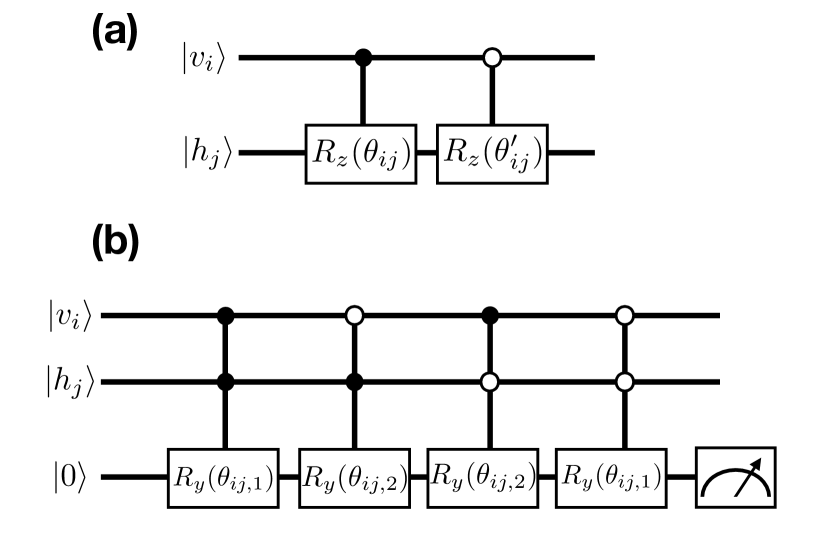
Figure 4: Quantum circuits for the coupling terms (a) $\exp(\mathrm{i}\sum_{i}W_{ij}^{I}\hat{v}^{z}_{i}\hat{h}^{z}_{j})$ and (b) $\exp(\sum_{i}W_{ij}^{R}\hat{v}^{z}_{i}\hat{h}^{z}_{j})$ between $i$-th visible and $j$-th hidden spins, .

Appendix B Ensemble Preparation of unitary RBM States

Here we discuss an ensemble preparation of the unitary RBM state without resorting to the probabilistic post-selection of hidden spins Hsieh et al. (2021). First we note that each term on the right hand side of Eq. 4 in the main text can be written as

$$\prescript{}{}{\langle+|}\left[e^{\hat{h}^{z}_{j}\left(m_{j}+\sum_{i}iW^{\text{I}}_{ij}\hat{v}^{z}_{i}\right)}\right]|+\rangle$$

$$= \sum_{s=\pm}\langle+|e^{m^{\text{R}}_{j}\hat{h}^{z}_{j}}|s\rangle\langle s|e^{\left(im^{\text{I}}_{j}+\sum_{i}iW^{\text{I}}_{ij}\hat{v}^{z}_{i}\right)\hat{h}^{z}_{j}}|+\rangle$$

$$= \sum_{s=\pm}R_{s}(m_{j}^{\text{R}})\langle s|e^{\left(im^{\text{I}}_{j}+\sum_{i}iW^{\text{I}}_{ij}\hat{v}^{z}_{i}\right)\hat{h}^{z}_{j}}|+\rangle,$$

where $R_{s}(m^{\text{R}}_{j})=\langle+|e^{m^{\text{R}}_{j}\hat{h}^{z}_{j}}|s\rangle$ can be computed classically as it only involves single qubit operation. Using Eq. B, we re-write Eq. 4 in the main text such that

$$|\Psi_{v}(\theta)\rangle = \sum_{s_{M}=\pm}\cdots\sum_{s_{1}=\pm}\frac{1}{N_{v}}\left(\prod_{j=1}^{M}R_{s_{j}}(m^{\text{R}}_{j})\right)$$

$$\prescript{}{}{\langle s_{M}|}\left[e^{\hat{h}^{z}_{M}\left(im^{\text{I}}_{M}+\sum_{i}iW^{\text{I}}_{iM}\hat{v}^{z}_{i}\right)}\right]|+\rangle\cdots$$

$$\prescript{}{}{\langle s_{1}|}\left[e^{\hat{h}^{z}_{1}\left(im^{\text{I}}_{1}+\sum_{i}iW^{\text{I}}_{i1}\hat{v}^{z}_{i}\right)}\right]|+\rangle\,\,e^{\sum_{i}b_{i}\hat{v}^{z}_{i}}|++\cdots\rangle_{v}$$

$$= \sum_{s_{M}=\pm}\cdots\sum_{s_{1}=\pm}\frac{N_{\vec{s}}}{N_{v}}\left(\prod_{j=1}^{M}R_{s_{j}}(m^{\text{R}}_{j})\right)|\Psi_{v}^{\vec{s}}(\theta)\rangle,$$

where $\vec{s}=[s_{1},\cdots,s_{M}]$ and $N_{\vec{s}}$ is the normalization to ensure $\langle{\Psi_{v}^{\vec{s}}}|{\Psi_{v}^{\vec{s}}}\rangle=1$. $|\Psi_{v}^{\vec{s}}(\theta)\rangle$ is a visible-spin wave function created by projecting hidden spins onto basis states $|s_{1}\cdots s_{M}\rangle_{h}$. Therefore the state preparation protocol given in Eq. B replaces the probabilistic post-selection of hidden spins with a summation over all possible $\vec{s}$ of hidden spins.

The expectation value of an observable $\hat{O}$ can be calculated

$$\langle\Psi_{v}(\theta)|\hat{O}|\Psi_{v}(\theta)\rangle$$ (19)

$$=\int dz|\langle{\mathbf{z}}|{\Psi_{v}(\theta)}\rangle|^{2}\left[\int dz^{\prime}O(z,z^{\prime})\frac{\langle{\mathbf{z}^{\prime}}|{\Psi_{v}(\theta)}\rangle}{\langle{\mathbf{z}}|{\Psi_{v}(\theta)}\rangle}\right].$$

The above equation suggests that the expectation value of an observable $\hat{O}$ can be turned into the average of the expression inside the square bracket if we can efficiently sample $z$ according to the probability density $|\langle{\mathbf{z}}|{\Psi_{v}(\theta)}\rangle|^{2}$.

Appendix C Variational imaginary time evolution

In the numerical examples of closed systems in Fig. 2 of the main text, the initial states are prepared as the ground states of the initial Hamiltonians before quantum quenches. The variational parameters of these initial wavefunctions are obtained via a variational quantum-classical imaginary time evolution (ITE) following the Stochastic Reconfiguration framework Sorella and Capriotti (2000). The update rule of the variational parameters in the hybrid ITE algorithm is

$$\dot{\theta}_{n}(\tau)=\sum_{m}A_{nm}^{-1}\,\text{Re}[f_{m}].$$ (20)

where $\tau$ denotes the imaginary time, the definitions of the covariance matrix $A$ and the force vector $f$ are the same as the real time algorithm (i.e. Eqs. (7) and (8)) in the main text. The parameters are updated iteratively

$$\theta_{n}(\tau+\delta\tau)=\theta_{n}(\tau)+\delta\tau A^{-1}\text{Re}[f]$$ (21)

where $\delta\tau$ is the imaginary time step. In our simulations, we use $\delta\tau=0.01$ for 2500 steps. At $\tau=0$, the variational RBM parameters are initialized as Gaussian random numbers with zero mean and variance of 0.01. The imaginary time evolution of the 14-spin 1D Ising and Heisenberg models used in the main text are shown in Fig. 5.

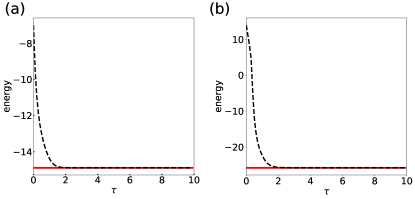
Figure 5: Imaginary time evolution of (a) 1D Ising model and (b) Heisenberg models. The solid lines are the exact ground-state energy. The dashed black lines represent the imaginary time evolution using the variational uRBM algorithm.

Appendix D Dynamics of Triangular Anti-Ferromagnetic Lattice

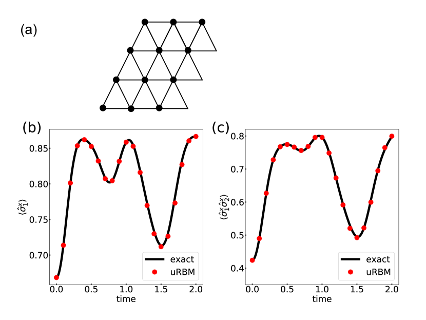
Figure 6: Time evolution in a two dimensional triangular anti-ferromagnetic Ising lattice induced by quantum quench. (a) Configuration of the triangular lattice with periodic boundary condition. (b) and (c) Results from uRBM algorithm (symbols) are compared to exact calculations (solids lines) for dynamics of transverse polarization and its correlation.

Here we consider the dynamics of a two dimensional triangular anti-ferromagnetic Ising (TAFI) model with periodic boundary condition, a system known for critical slow down for a range of magnetic fields. The Hamiltonian is given by

$$\hat{H} = -h\sum_{i}\hat{\sigma}_{i}^{x}+\sum_{<ij>}\hat{\sigma}_{i}^{z}\hat{\sigma}_{j}^{z},$$ (22)

where $h$ denotes the strength of the transverse field. A schematic of the triangular lattice is shown in Fig. 6 (a). We perform a quantum quench by instantaneously changing the transverse field from $h=0.5$ to $h=1.0$ at $t=0$. We use $\delta t=0.0005$ and $\alpha=M/N=8$ in our simulations. Figs. 6 (b) and (c) shows the dynamics of transverse spin polarization $\langle\sigma_{1}^{x}\rangle$ and its correlation $\langle\sigma_{1}^{x}\sigma_{2}^{x}\rangle$ of a 12-spin triangular lattice. The good agreement with exact results for this more challenging example further demonstrate the capability of the uRBM algorithm in capturing quantum many-body dynamics.

Appendix E Ergodicity Problem in Triangular Anti-Ferromagnetic Lattice

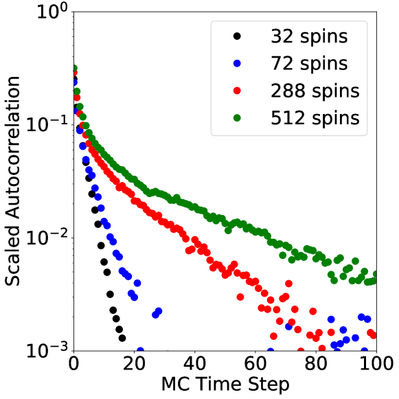
Figure 7: Autocorrelation of a two dimensional triangular anti-ferromagnetic Ising model as a function of Monte Carlo step number for $O=\sigma^{z}_{(0,0)}\sigma^{z}_{(L/2,L/2)}$. $y$-aixs is scaled by $\langle O(\tau=0)O(\tau=0)\rangle$ to ensure that maximum value is unity.

Here we investigate the ergodicity issue of TAFI model in the classical limit (i.e. $h=0$). The classical TAFI model is one of the simplest examples of a frustrated magnet hosting a spin liquid phase at zero temperature Blote and Hilborst (1982). The large correlation lengths associated with scale invariant behavior close to such phases lead to complex energy landscapes and a poor performance of simple Metropolis like updates in Monte Carlo. Although it is possible in special cases to develop efficient cluster algorithms, most frustrated spin systems do not lend themselves to such methods. This is made explicit for the TAFI in a uniform transverse field in Ref. Biswas et al. (2016), where the authors develop a specialized cluster algorithm to study the physics at low transverse fields. To quantify the performance of standard Metropolis updates on the classical TAFI, we calculate an autocorrelation function of the spin correlation on lattice sites with maximal separation, i.e. $\sigma^{z}_{(0,0)}\sigma^{z}_{(L/2,L/2)}$, where the subscripts denote the spin position and $L$ is the lattice length in each dimension. This is shown for a range of sizes in Fig. 7 and we see that the time to equilibrium grows with system size. As qualitative features of the ground state phase remain similar at finite transverse fields, we expect that similarly long autocorrelation times would be seen in that case as well, evidence for the same is shown explicitly in Ref. Biswas et al. (2016). With direct sampling in quantum computers, we would circumvent this ergodicity issue.

Appendix F Numerical Simulations with Gaussian Noise

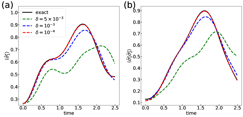
Figure 8: Noisy simulations of a 6-spin 1D Ising lattice induced by quantum quench. To account for the imperfections of actual quantum devices, random Gaussian noises with standard deviation $\delta$ are added to the covariance matrix, $A$ and the force vector $f$. Results from noisy uRBM simulations (dahsed lines) are compared to exact calculations (black solid lines) for dynamics of transverse polarization and its correlation.

To assess the robustness of the neural-network variational algorithm against imperfections of near-term quantum computers and errors due to finite number of measurements, we perform noisy simulations by adding random Gaussian noise into the matrix elements of the covariance matrix, $A$ and the force vector $f$ at each time step $\delta t$. We use a Gaussian random number of zero mean and standard deviation of $\delta$. We perform noisy simulation of a 6-spin 1D Ising model (see Eq. 10 of main text for Hamiltonian)and study its dynamics upon quantum quench when the transverse field is changed from $h_{i}=0.5$ to $h_{f}=1.0$ at $t=0$, the time evolution of transverse polarization and its correlation is shown in Fig. 8. It can be seen that our algorithm is robust against small errors, but as the magnitude of the noise increases, the quantum dynamics start to deviate significantly from the exact dynamics.

As the performance of quantum computers improves rapidly in recent years, error rates of $10^{-4}-10^{-3}$ used in Fig. 8 can be expected the near-future. Particularly single-qubit gate fidelity of $99.9999\%$ Harty et al. (2014) and two-qubit gate fidelity of $99.9\%$ Ballance et al. (2016); Gaebler et al. (2016) have already been demonstrated in trapped ion quantum computer.

Appendix G Derivations of wavefunction derivatives

The derivative of $|\Psi_{v}(\theta)\rangle$ can be written as

$$\left|\frac{\partial\Psi_{v}}{\partial\theta_{n}}\right\rangle = \frac{{}_{h}\langle++\dots+|\partial_{\theta_{n}}\tilde{\Psi}_{vh}\rangle}{\tilde{N}_{v}}$$

$$- Re\left(\frac{\langle\tilde{\Psi}_{vh}|}{\tilde{N}_{v}}\hat{P}_{+}^{(h)}\frac{|\partial_{\theta_{n}}\tilde{\Psi}_{vh}\rangle}{\tilde{N}_{v}}\right)\frac{{}_{h}\langle++\dots+|{\tilde{\Psi}_{vh}}\rangle}{\tilde{N}_{v}},$$

where $|\tilde{\Psi}_{vh}(\theta)\rangle=e^{\hat{H}_{RBM}(\theta)}|++\dots+\rangle_{vh}$ is the unnormalized wavefunction and $N_{v}=\sqrt{\langle\Psi_{vh}(\theta)|P^{(h)}_{+}|\Psi_{vh}(\theta)\rangle}$. $\hat{H}_{RBM}(\theta,h)$ is the RBM Hamiltonian with the hidden spins $\hat{h}^{z}_{j}$ replaced with binary values of $\pm 1$. The derivatives of $|\tilde{\Psi}_{vh}(\theta)\rangle$ are in turn given by

$$\frac{\partial|\tilde{\Psi}_{vh}\rangle}{\partial b^{R}_{i}} = \hat{v}^{z}_{i}|\tilde{\Psi}_{vh}\rangle,$$ (24)

$$\frac{\partial|\tilde{\Psi}_{vh}\rangle}{\partial m^{R}_{j}} = \tanh\left(m_{j}+\sum_{i}W_{ij}\hat{v}^{z}_{i}\right)|\tilde{\Psi}_{vh}\rangle,$$

$$\frac{\partial|\tilde{\Psi}_{vh}\rangle}{\partial W^{R}_{ij}} = \hat{v}^{z}_{i}\tanh\left(m_{j}+\sum_{i}W_{ij}\hat{v}^{z}_{i}\right)|\tilde{\Psi}_{vh}\rangle,$$

$$\frac{\partial|\tilde{\Psi}_{vh}\rangle}{\partial b^{I}_{i}} = i\hat{v}^{z}_{i}|\tilde{\Psi}_{vh}\rangle,$$

$$\frac{\partial|\tilde{\Psi}_{vh}\rangle}{\partial m^{I}_{j}} = i\tanh\left(m_{j}+\sum_{i}W_{ij}\hat{v}^{z}_{i}\right)|\tilde{\Psi}_{vh}\rangle,$$

$$\frac{\partial|\tilde{\Psi}_{vh}\rangle}{\partial W^{I}_{ij}} = i\hat{v}^{z}_{i}\tanh\left(m_{j}+\sum_{i}W_{ij}\hat{v}^{z}_{i}\right)|\tilde{\Psi}_{vh}\rangle.$$

Substituting Eqs. G-24 into in the derivative operator, $O_{n}=\frac{\partial\ln|\Psi_{v}\rangle}{\partial\theta_{n}}$, we arrive at Eq.(9) in the main text.

Appendix H Measuring Derivatives in Quantum Circuits

Here we explain how to measure the matrix elements of the covariance matrix $A$ and force vector $f$. Since $[\hat{O}_{n},\hat{v}^{z}_{i}]=0$, the expectation values of $\langle\hat{O}^{\dagger}_{n}\hat{O}_{m}\rangle_{v}$ can be obtained by measuring the visible spins in the $z$-basis

$$\langle\hat{O}^{\dagger}_{n}\hat{O}_{m}\rangle_{v}$$

$$= \langle\Psi_{v}(\theta)|\hat{O}^{\dagger}_{n}\hat{O}_{m}|\Psi_{v}(\theta)\rangle$$

$$= \sum_{\mathbf{z}_{v}}|\langle\Psi_{v}(\theta)|\mathbf{z}_{v}\rangle|^{2}\hat{O}^{\dagger}_{n}(\mathbf{z}_{v})\hat{O}_{m}(\mathbf{z}_{v})$$

$$\xrightarrow[\text{according to }P_{v}(\mathbf{z}_{v})]{\text{Monte Carlo sampling}}\sum_{k=1}^{N_{\text{exp}}}\frac{\hat{O}^{\dagger}_{n}(\mathbf{z}_{v}^{k})\hat{O}_{m}(\mathbf{z}_{v}^{k})}{N_{\text{exp}}},$$

where we have inserted the completeness relation, $\sum_{\mathbf{z}_{v}}|{\mathbf{z}_{v}}\rangle\langle{\mathbf{z}_{v}}|$, into the second line. Here $P_{v}(\mathbf{z}_{v})=|\langle{\Psi_{v}(\theta)}|{\mathbf{z}_{v}}\rangle|^{2}$ is a probability density, $\mathbf{z}_{v}=[z_{v,1},\cdots,z_{v,N}]$ is a length-$N$ binary string, and $\hat{O}_{n}$ is defined in Eq. 9 of the main text, with the visible spin operators replaced by $\mathbf{z}_{v}$. $N_{\text{exp}}$ samples of [$\mathbf{z}_{v}^{(k=1)}\cdots\mathbf{z}_{v}^{(k=N_{\text{exp}})}$] are obtained from the quantum circuit to estimate $\hat{O}^{\dagger}_{n}(\mathbf{z}_{v}^{k})\hat{O}_{m}(\mathbf{z}_{v}^{k})$, according to the third line (the Monte Carlo method) in equation above. The expression $\hat{O}^{\dagger}_{n}(\mathbf{z}_{v}^{k})\hat{O}_{m}(\mathbf{z}_{v}^{k})$ can be evaluated efficiently once a computational state $\mathbf{z}^{k}_{v}$ is specified. $\langle\hat{O}_{n}\rangle_{v}$ can be similarly calculated.

The evaluation of $\langle\hat{O}^{\dagger}_{m}\hat{H}\rangle_{v}$ is more complicated,

$$\langle\hat{O}^{\dagger}_{m}\hat{H}\rangle_{v}$$

$$= \langle\Psi_{v}(\theta)|\hat{O}^{\dagger}_{m}\hat{H}|\Psi_{v}(\theta)\rangle$$

$$= \sum_{\mathbf{z}_{v},\tilde{\mathbf{z}}_{v}}\langle{\Psi_{v}(\theta)}|{\mathbf{z}_{v}}\rangle O^{\dagger}_{m}(\mathbf{z}_{v})\hat{H}(\mathbf{z}_{v},\tilde{\mathbf{z}}_{v})\langle{\tilde{\mathbf{z}}_{v}}|{\Psi_{v}(\theta)}\rangle$$

$$= \sum_{\mathbf{z}_{v}}|\langle{\Psi_{v}(\theta)}|{\mathbf{z}_{v}}\rangle|^{2}\left(\sum_{\tilde{\mathbf{z}}_{v}}\hat{O}^{\dagger}_{m}(\mathbf{z}_{v})\hat{H}(\mathbf{z}_{v},\tilde{\mathbf{z}}_{v})\frac{\langle{\tilde{\mathbf{z}}_{v}}|{\Psi_{v}(\theta)}\rangle}{\langle{\mathbf{z}_{v}}|{\Psi_{v}(\theta)}\rangle}\right),$$

$$\xrightarrow[\text{according to }P_{v}(\mathbf{z}_{v})]{\text{Monte Carlo sampling}}\sum_{k=1}^{N_{\text{exp}}}\frac{1}{N_{\text{exp}}}\times$$

$$\,\,\,\,\,\,\,\,\,\,\,\,\,\,\,\,\,\,\,\,\,\,\,\,\,\,\,\,\,\,\,\,\,\,\,\left(\sum_{j}\hat{O}^{\dagger}_{m}(\mathbf{z}^{k}_{v})\hat{H}(\mathbf{z}^{k}_{v},\tilde{\mathbf{z}}^{k,j}_{v})\frac{\langle{\tilde{\mathbf{z}}^{k,j}_{v}}|{\Psi_{v}(\theta)}\rangle}{\langle{\mathbf{z}^{k}_{v}}|{\Psi_{v}(\theta)}\rangle}\right),$$

where $\hat{H}(\mathbf{z}_{v}^{k},\tilde{\mathbf{z}}^{k,j}_{v})=\langle\mathbf{z}^{k}_{v}|\hat{H}|\tilde{\mathbf{z}}^{k,j}_{v}\rangle$. For physical systems, the Hamiltonian, $\hat{H}=\sum_{l}w_{l}\hat{P}_{l}$, is a linear combination of Pauli strings, i.e. $\hat{H}$ is a sparse matrix such that each computational state $|\mathbf{z}^{k}_{v}\rangle$ is only connected to a few other states $|\tilde{\mathbf{z}}_{v}^{k,j}\rangle$. The expression in the bracket of the third line of Eq. H can then be evaluated classically efficiently.

Appendix I Gradients of uRBM Parameters

Here we show that the proposed uRBM algorithm does not suffer from the ‘barren plateau’ issue that affects many variational quantum algorithms McClean et al. (2018). In Fig. 9 we plot the norms of the force vector, $f$, and the gradient, $A^{-1}f$, as a function of system size, both quantities are normalized by the total number of variational parameters. We consider a 1D transverse field Ising model (panels (a) and (b)) and a 1D Heisenberg model in longitudinal field (panels (c) and (d)) with periodic boundary condition, both with magnetic field strength $h=1.0$. The number of hidden spins is fixed at $M=6$. The RBM parameters are randomly initialized as Gaussian variables with variance of 0.01, the blue and red lines in Fig. 9 denote the average and minimum of 100 random initializations, respectively.

The force vector, $f$, is simply the gradient vector of the energy function, $E_{\theta}=\langle\Psi_{v}|(\theta)H_{s}|\Psi_{v}\rangle(\theta)$, whereas the real and imaginary parts of $A^{-1}f$ dictate the parameter update in imaginary and real time evolution (see Eq. 6 in main text and Eq. 20 above), respectively. From Fig. 9, we can clearly see that both $f$ and $A^{-1}f$ do not decay exponentially with system size, indicating the uRBM algorithm does not suffer from the vanishing gradient ( or ‘barren plateau’) issue.

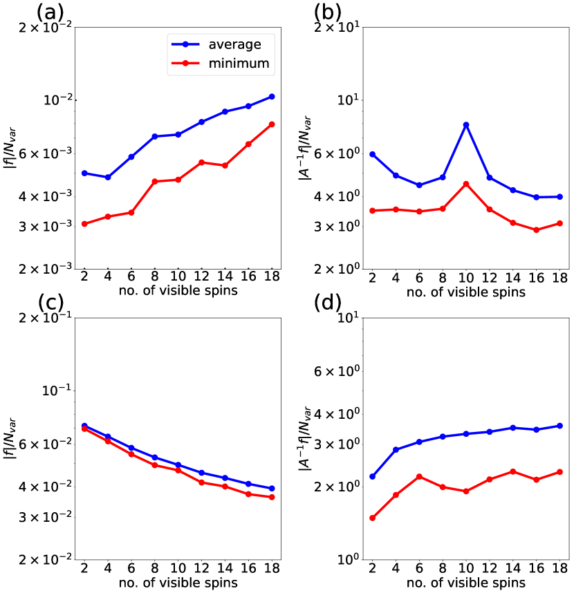
Figure 9: The norms of $f$ and $A^{-1}f$ as a function of system size for a 1D transverse field Ising model ((a) and (b)) and a 1D Heisenberg model in longitudinal field ((c) and (d)). The norms are normalized by the number of variational parameters. The blue and red lines denote the average and minimum from 100 random initializations, respectively.

Appendix J Stochastic Schrödinger Equation

The dynamics of an open quantum system coupled to a Markovian bath can be described by an ensemble of pure state trajectories under continuous measurement Dalibard et al. (1992); Carmichael (1993). The stochastic differential equation governing the evolution of the pure state trajectory can be written as

$$d|\psi(t)\rangle = -\mathrm{i}\hat{H}_{eff}|\psi(t)\rangle dt+$$

$$\sum_{k}\Big{(}\frac{\hat{L}_{k}|\psi(t)\rangle}{\|\hat{L}_{k}|\psi(t)\rangle\|}-|\psi(t)\rangle\Big{)}dN_{k}(t),$$

where the non-Hermitian effective Hamiltonian

$$\hat{H}_{eff}=\hat{H}_{s}-\frac{\mathrm{i}}{2}\sum_{k}(\hat{L}_{k}\hat{L}_{k}^{\dagger}-\langle\hat{L}_{k}\hat{L}_{k}^{\dagger}\rangle),$$ (28)

describes the deterministic evolution of the trajectory. The first term on the right hand side of Eq. 28 is the usual system Hamiltonian, and the non-Hermitian part (terms in bracket) describes the damping process. The terms $\langle\hat{L}_{k}\hat{L}_{k}^{\dagger}\rangle=\langle\psi(t)|\hat{L}_{k}\hat{L}_{k}^{\dagger}|\psi(t)\rangle$ ensure normalization of the wavefunction. The deterministic evolution is interrupted by instantaneous changes to the wavefunction, $|\psi\rangle\rightarrow\frac{\hat{L}_{k}|\psi\rangle}{\|\hat{L}_{k}|\psi\rangle\|}$, the so-called quantum jumps described by the second term on the right hand side of Eq. J. The random numbers $dN_{k}(t)$ associated to the jumps take on the values of $0$ or $1$ and have expectation values of

$$E[dN_{k}(t)]=\langle\psi(t)|\hat{L}_{k}^{\dagger}\hat{L}_{k}|\psi(t)\rangle dt.$$ (29)

$E[dN_{k}(t)]$ represents the probability of a quantum jump associated to the Linblad operator $\hat{L}_{k}$, the total jump probability is thus given by $\sum_{k}E[dN_{k}(t)]$.

Next we describe how the stochastic Schrödinger equation can be simulated using variational algorithm described in the main text. We first assume that the wavefunction at time $t$, $|\psi(t)\rangle$, can be represented by a parametrized ansatz $|\Psi(\theta)\rangle$ prepared in a quantum circuit. Between quantum jumps, the deterministic part of the stochastic Schrödinger can then be simulated with Eqs. 6-8 in the main text, but replacing the system Hamiltonian with the effective Hamiltonian $H_{eff}$. To realize a quantum jump associated with $\hat{L}_{k}=\sigma_{k}^{+}$, we first note that the raising operator can be written as $\hat{\sigma}^{+}_{k}=\text{e}^{-\tau\hat{H}_{k}}\text{e}^{-\mathrm{i}\frac{\pi}{2}\hat{\sigma}^{x}_{k}}$ for large enough $\tau$ Endo et al. (2020) and $\hat{H}_{k}=|0\rangle_{k}\langle 0|$. Then the quantum jump can be realized in a quantum circuit by evolving the quantum state s $\sigma^{x}_{k}$ for duration $\frac{\pi}{2}$. Then we propagate the state by imaginary time evolution under $\hat{H}_{k}$ for $\tau$. In our simulations we use $\tau=20$ and time step of $\delta\tau=0.01$.

References

- Bernien et al. (2017) Hannes Bernien, Sylvain Schwartz, Alexander Keesling, Harry Levine, Ahmed Omran, Hannes Pichler, Soonwon Choi, Alexander S Zibrov, Manuel Endres, Markus Greiner, and Others, “Probing many-body dynamics on a 51-atom quantum simulator,” Nature 551, 579–584 (2017).
- Celi et al. (2020) Alessio Celi, Beno^ Vermersch, Oscar Viyuela, Hannes Pichler, Mikhail D Lukin, and Peter Zoller, “Emerging Two-Dimensional Gauge Theories in Rydberg Configurable Arrays,” Physical Review X 10, 21057 (2020).
- Sala et al. (2020) Pablo Sala, Tibor Rakovszky, Ruben Verresen, Michael Knap, and Frank Pollmann, “Ergodicity breaking arising from Hilbert space fragmentation in dipole-conserving Hamiltonians,” Physical Review X 10, 11047 (2020).
- Yang et al. (2020) Zhi-Cheng Yang, Fangli Liu, Alexey V Gorshkov, and Thomas Iadecola, “Hilbert-space fragmentation from strict confinement,” Physical Review Letters 124, 207602 (2020).
- De Tomasi et al. (2019) Giuseppe De Tomasi, Daniel Hetterich, Pablo Sala, and Frank Pollmann, “Dynamics of strongly interacting systems: From Fock-space fragmentation to many-body localization,” Physical Review B 100, 214313 (2019).
- Nandkishore and Hermele (2019) Rahul M Nandkishore and Michael Hermele, “Fractons,” Annual Review of Condensed Matter Physics 10, 295–313 (2019).
- Chamon (2005) Claudio Chamon, “Quantum glassiness in strongly correlated clean systems: an example of topological overprotection,” Physical review letters 94, 40402 (2005).
- Alet and Laflorencie (2018) Fabien Alet and Nicolas Laflorencie, “Many-body localization: An introduction and selected topics,” Comptes Rendus Physique 19, 498–525 (2018).
- Pal and Huse (2010) Arijeet Pal and David A Huse, “Many-body localization phase transition,” Physical review b 82, 174411 (2010).
- Nandkishore and Huse (2015) Rahul Nandkishore and David A Huse, “Many-body localization and thermalization in quantum statistical mechanics,” Annu. Rev. Condens. Matter Phys. 6, 15–38 (2015).
- Suzuki (1993) Masuo Suzuki, Quantum Monte Carlo methods in condensed matter physics (World scientific, 1993).
- Ceperley and Alder (1986) David Ceperley and Berni Alder, “Quantum monte carlo,” Science 231, 555–560 (1986).
- Bishop and Farnell (2000) R F Bishop and Damian J J Farnell, “Marshall-Peierls sign rules, the quantum monte carlo method, and frustration,” in Recent Progress In Many-Body Theories (World Scientific, 2000) pp. 457–460.
- Troyer and Wiese (2005) Matthias Troyer and Uwe-Jens Wiese, “Computational complexity and fundamental limitations to fermionic quantum Monte Carlo simulations,” Physical review letters 94, 170201 (2005).
- Carleo et al. (2017) Giuseppe Carleo, Lorenzo Cevolani, Laurent Sanchez-Palencia, and Markus Holzmann, “Unitary dynamics of strongly interacting Bose gases with the time-dependent variational Monte Carlo method in continuous space,” Physical Review X 7, 31026 (2017).
- Ido et al. (2015) Kota Ido, Takahiro Ohgoe, and Masatoshi Imada, “Time-dependent many-variable variational Monte Carlo method for nonequilibrium strongly correlated electron systems,” Physical Review B 92, 245106 (2015).
- Biswas et al. (2016) Sounak Biswas, Geet Rakala, and Kedar Damle, “Quantum cluster algorithm for frustrated Ising models in a transverse field,” Physical Review B 93, 235103 (2016).
- Syljuåsen and Sandvik (2002) Olav F Syljuåsen and Anders W Sandvik, “Quantum Monte Carlo with directed loops,” Physical Review E 66, 46701 (2002).
- Yan et al. (2019) Zheng Yan, Yongzheng Wu, Chenrong Liu, Olav F Syljuåsen, Jie Lou, and Yan Chen, “Sweeping cluster algorithm for quantum spin systems with strong geometric restrictions,” Physical Review B 99, 165135 (2019).
- Carleo and Troyer (2017) Giuseppe Carleo and Matthias Troyer, “Solving the quantum many-body problem with artificial neural networks,” Science 355, 602–606 (2017).
- Nagy and Savona (2019) Alexandra Nagy and Vincenzo Savona, “Variational quantum monte carlo method with a neural-network ansatz for open quantum systems,” Phys. Rev. Lett. 122, 250501 (2019).
- Glasser et al. (2018) Ivan Glasser, Nicola Pancotti, Moritz August, Ivan D Rodriguez, and J Ignacio Cirac, “Neural-network quantum states, string-bond states, and chiral topological states,” Phys. Rev. X 8, 11006 (2018).
- Schmitt and Heyl (2019) Markus Schmitt and Markus Heyl, “Quantum many-body dynamics in two dimensions with artificial neural networks,” Physical Review Letters 125, 100503 (2019).
- Gutiérrez and Mendl (2019) Irene López Gutiérrez and Christian B. Mendl, “Real time evolution with neural-network quantum states,” (2019), arXiv:1912.08831 .
- Deng et al. (2017) Dong-Ling Deng, Xiaopeng Li, and S Das Sarma, “Machine learning topological states,” Phys. Rev. B 96, 195145 (2017).
- Sarma et al. (2019) Sankar Das Sarma, Dong-Ling Deng, and Lu-Ming Duan, “Machine learning meets quantum physics,” Physics Today 72, 48 (2019).
- Hartmann and Carleo (2019) Michael J. Hartmann and Giuseppe Carleo, “Neural-Network Approach to Dissipative Quantum Many-Body Dynamics,” Physical Review Letters 122, 250502 (2019), arXiv:1902.05131 .
- Vicentini et al. (2019) Filippo Vicentini, Alberto Biella, Nicolas Regnault, and Cristiano Ciuti, “Variational neural-network ansatz for steady states in open quantum systems,” Physical review letters 122, 250503 (2019).
- Yoshioka and Hamazaki (2019) Nobuyuki Yoshioka and Ryusuke Hamazaki, “Constructing neural stationary states for open quantum many-body systems,” Phys. Rev. B 99, 214306 (2019).
- Preskill (2018) John Preskill, “Quantum Computing in the NISQ era and beyond,” Quantum 2, 79 (2018).
- Arute et al. (2019) Frank Arute, Kunal Arya, Ryan Babbush, Dave Bacon, Joseph C. Bardin, Rami Barends, Rupak Biswas, Sergio Boixo, Fernando G. S. L. Brandao, David A. Buell, Brian Burkett, Yu Chen, Zijun Chen, Ben Chiaro, Roberto Collins, William Courtney, Andrew Dunsworth, Edward Farhi, Brooks Foxen, Austin Fowler, Craig Gidney, Marissa Giustina, Rob Graff, Keith Guerin, Steve Habegger, Matthew P. Harrigan, Michael J. Hartmann, Alan Ho, Markus Hoffmann, Trent Huang, Travis S. Humble, Sergei V. Isakov, Evan Jeffrey, Zhang Jiang, Dvir Kafri, Kostyantyn Kechedzhi, Julian Kelly, Paul V. Klimov, Sergey Knysh, Alexander Korotkov, Fedor Kostritsa, David Landhuis, Mike Lindmark, Erik Lucero, Dmitry Lyakh, Salvatore Mandrà, Jarrod R. McClean, Matthew McEwen, Anthony Megrant, Xiao Mi, Kristel Michielsen, Masoud Mohseni, Josh Mutus, Ofer Naaman, Matthew Neeley, Charles Neill, Murphy Yuezhen Niu, Eric Ostby, Andre Petukhov, John C. Platt, Chris Quintana, Eleanor G. Rieffel, Pedram Roushan, Nicholas C. Rubin, Daniel Sank, Kevin J. Satzinger, Vadim Smelyanskiy, Kevin J. Sung, Matthew D. Trevithick, Amit Vainsencher, Benjamin Villalonga, Theodore White, Z. Jamie Yao, Ping Yeh, Adam Zalcman, Hartmut Neven, and John M. Martinis, “Quantum supremacy using a programmable superconducting processor,” Nature 574, 505–510 (2019).
- McClean et al. (2016) Jarrod R McClean, Jonathan Romero, Ryan Babbush, and Alán Aspuru-Guzik, “The theory of variational hybrid quantum-classical algorithms,” New J. Phys. 18, 23023 (2016).
- Peruzzo et al. (2014) Alberto Peruzzo, Jarrod McClean, Peter Shadbolt, Man Hong Yung, Xiao Qi Zhou, Peter J. Love, Alán Aspuru-Guzik, and Jeremy L. O’Brien, “A variational eigenvalue solver on a photonic quantum processor,” Nature Communications 5 (2014), 10.1038/ncomms5213.
- Farhi et al. (2014) Edward Farhi, Jeffrey Goldstone, and Sam Gutmann, “A quantum approximate optimization algorithm,” arXiv preprint arXiv:1411.4028 (2014).
- Kandala et al. (2017) Abhinav Kandala, Antonio Mezzacapo, Kristan Temme, Maika Takita, Markus Brink, Jerry M Chow, and Jay M Gambetta, “Hardware-efficient variational quantum eigensolver for small molecules and quantum magnets,” Nature 549, 242 (2017).
- Hempel et al. (2018) Cornelius Hempel, Christine Maier, Jonathan Romero, Jarrod McClean, Thomas Monz, Heng Shen, Petar Jurcevic, Ben P Lanyon, Peter Love, Ryan Babbush, and Others, “Quantum chemistry calculations on a trapped-ion quantum simulator,” Phys. Rev. X 8, 31022 (2018).
- Colless et al. (2018) J. I. Colless, V. V. Ramasesh, D. Dahlen, M. S. Blok, M. E. Kimchi-Schwartz, J. R. McClean, J. Carter, W. A. De Jong, and I. Siddiqi, “Computation of Molecular Spectra on a Quantum Processor with an Error-Resilient Algorithm,” Physical Review X 8, 11021 (2018).
- Li and Benjamin (2017) Ying Li and Simon C. Benjamin, “Efficient Variational Quantum Simulator Incorporating Active Error Minimization,” Physical Review X 7, 021050 (2017).
- Yuan et al. (2019) Xiao Yuan, Suguru Endo, Qi Zhao, Ying Li, and Simon C. Benjamin, “Theory of variational quantum simulation,” Quantum 3, 191 (2019).
- Heya et al. (2019) Kentaro Heya, Ken M Nakanishi, Kosuke Mitarai, and Keisuke Fujii, “Subspace Variational Quantum Simulator,” (2019), arXiv:1904.08566 .
- Lee et al. (2021) Chee-Kong Lee, Jonathan Wei Zhong Lau, Liang Shi, and Leong Chuan Kwek, “Simulating Energy Transfer in Molecular Systems with Digital Quantum Computers,” (2021), arXiv:2101.06879 .
- Endo et al. (2020) Suguru Endo, Jinzhao Sun, Ying Li, Simon C. Benjamin, and Xiao Yuan, “Variational Quantum Simulation of General Processes,” Physical Review Letters 125, 010501 (2020), arXiv:1812.08778 .
- Hsieh et al. (2021) Chang Yu Hsieh, Qiming Sun, Shengyu Zhang, and Chee Kong Lee, “Unitary-coupled restricted Boltzmann machine ansatz for quantum simulations,” npj Quantum Information 7 (2021).
- Xia and Kais (2018) Rongxin Xia and Sabre Kais, “Quantum machine learning for electronic structure calculations,” Nat. Commun. 9, 4195 (2018).
- Carleo et al. (2012) Giuseppe Carleo, Federico Becca, Marco Schiró, and Michele Fabrizio, “Localization and Glassy Dynamics Of Many-Body Quantum Systems,” Scientific Reports 2, 243 (2012).
- Carleo et al. (2014) Giuseppe Carleo, Federico Becca, Laurent Sanchez-Palencia, Sandro Sorella, and Michele Fabrizio, “Light-cone effect and supersonic correlations in one- and two-dimensional bosonic superfluids,” Physical Review A 89, 031602 (2014).
- Becca and Sorella (2017) Federico Becca and Sandro Sorella, Quantum Monte Carlo Approaches for Correlated Systems (Cambridge University Press, 2017).
- Luitz et al. (2015) David J Luitz, Nicolas Laflorencie, and Fabien Alet, “Many-body localization edge in the random-field Heisenberg chain,” Physical Review B 91, 81103 (2015).
- Breuer and Petruccione (2007) Heinz-Peter Breuer and Francesco Petruccione, The Theory of Open Quantum Systems (Oxford University Press, 2007).
- Dalibard et al. (1992) Jean Dalibard, Yvan Castin, and Klaus Mølmer, “Wave-function approach to dissipative processes in quantum optics,” Physical Review Letters 68, 580–583 (1992).
- Carmichael (1993) H. J. Carmichael, “Quantum trajectory theory for cascaded open systems,” Physical Review Letters 70, 2273–2276 (1993).
- Fink et al. (2018) Thomas Fink, Anne Schade, Sven Höfling, Christian Schneider, and Ataç Imamoglu, “Signatures of a dissipative phase transition in photon correlation measurements,” Nature Physics 14, 365–369 (2018).
- Raftery et al. (2014) J. Raftery, D. Sadri, S. Schmidt, H. E. Türeci, and A. A. Houck, “Observation of a Dissipation-Induced Classical to Quantum Transition,” Physical Review X 4, 031043 (2014).
- McClean et al. (2018) Jarrod R. McClean, Sergio Boixo, Vadim N. Smelyanskiy, Ryan Babbush, and Hartmut Neven, “Barren plateaus in quantum neural network training landscapes,” Nature communications 9, 4812 (2018).
- Zen et al. (2020a) Remmy Zen, Long My, Ryan Tan, Frédéric Hébert, Mario Gattobigio, Christian Miniatura, Dario Poletti, and Stéphane Bressan, “Transfer learning for scalability of neural-network quantum states,” Physical Review E 101, 053301 (2020a).
- Zen et al. (2020b) Remmy Zen, Long My, Ryan Tan, Frederic Hebert, Mario Gattobigio, Christian Miniatura, Dario Poletti, and Stephane Bressan, “Finding Quantum Critical Points with Neural-Network Quantum States,” (2020b), arXiv:2002.02618 .
- McArdle et al. (2019) Sam McArdle, Tyson Jones, Suguru Endo, Ying Li, Simon C. Benjamin, and Xiao Yuan, “Variational ansatz-based quantum simulation of imaginary time evolution,” npj Quantum Information 5 (2019).
- Brown et al. (2016) Kenneth R Brown, Jungsang Kim, and Christopher Monroe, “Co-designing a scalable quantum computer with trapped atomic ions,” npj Quantum Inf. 2, 16034 (2016).
- Bruzewicz et al. (2019) Colin D Bruzewicz, John Chiaverini, Robert McConnell, and Jeremy M Sage, “Trapped-ion quantum computing: Progress and challenges,” Appl. Phys. Rev. 6, 21314 (2019).
- Gao and Duan (2017) Xun Gao and Lu Ming Duan, “Efficient representation of quantum many-body states with deep neural networks,” Nature Communications 8, 1–5 (2017), arXiv:1701.05039 .
- Carleo et al. (2018) Giuseppe Carleo, Yusuke Nomura, and Masatoshi Imada, “Constructing exact representations of quantum many-body systems with deep neural networks,” Nature Communications 9, 5322 (2018).
- Liu et al. (2020) Zidu Liu, L. M. Duan, and Dong-Ling Deng, “Solving Quantum Master Equations with Deep Quantum Neural Networks,” (2020), arXiv:2008.05488 .
- Lin et al. (2020) Sheng-Hsuan Lin, Rohit Dilip, Andrew G. Green, Adam Smith, and Frank Pollmann, “Real- and imaginary-time evolution with compressed quantum circuits,” (2020), arXiv:2008.10322 .
- Sorella and Capriotti (2000) Sandro Sorella and Luca Capriotti, “Green function Monte Carlo with stochastic reconfiguration: An effective remedy for the sign problem,” Physical Review B 61, 2599–2612 (2000).
- Blote and Hilborst (1982) H W J Blote and H J Hilborst, “Roughening transitions and the zero-temperature triangular Ising antiferromagnet,” Journal of Physics A: Mathematical and General 15, L631 (1982).
- Harty et al. (2014) T P Harty, D T C Allcock, C J Ballance, L Guidoni, H A Janacek, N M Linke, D N Stacey, and D M Lucas, “High-Fidelity Preparation, Gates, Memory, and Readout of a Trapped-Ion Quantum Bit,” Phys. Rev. Lett. 113, 220501 (2014).
- Ballance et al. (2016) C J Ballance, T P Harty, N M Linke, M A Sepiol, and D M Lucas, “High-Fidelity Quantum Logic Gates Using Trapped-Ion Hyperfine Qubits,” Phys. Rev. Lett. 117, 60504 (2016).
- Gaebler et al. (2016) J P Gaebler, T R Tan, Y Lin, Y Wan, R Bowler, A C Keith, S Glancy, K Coakley, E Knill, D Leibfried, and D J Wineland, “High-Fidelity Universal Gate Set for Ion Qubits,” Phys. Rev. Lett. 117, 60505 (2016).