Curvature Scalarization of Black Holes in $f(R)$ Gravity

Abstract

We consider $f(R)$ gravity theories in the presence of a scalar field minimally coupled to gravity with a self-interacting potential. When the scalar field backreacts to the metric we find at large distances scalarized Schwarzschild-AdS and Schwarzschild-AdS-like black hole solutions. At small distances due to strong curvature effects and the scalar dynamis we find a rich structure of scalarized black hole solutions. When the scalar field is conformally coupled to gravity we also find scalarized black hole solutions at small distances.

I Introduction

The study of black hole solutions with scalar hair is a very interesting aspect of General Relativity (GR) and had attracted a lot of interest. These hairy black holes are solutions generated from a modified Einstein-Hilbert action in which a scalar field coupled to gravity is introduced. However, these solutions in order the scalar field to be regular on the horizon and well behaved at large distances have to obey the powerful no-hair theorems. The first hairy black hole solutions of GR were found in asymptotically flat spacetimes BBMB but it was realized that the scalar field was divergent on the horizon and stability analysis shown that these solutions were unstable bronnikov . Therefore, a regularization procedure has to be found and make the scalar field regular on the horizon. The easiest way to comply with this requirement is to introduce a cosmological constant making the scalar field regular on the horizon hiding all possible divergencies behind the horizon.

One of the first hairy black hole solution was discussed in Martinez:1996gn which was a generalization of the black hole solution in (2+1)-dimensions introduced in Banados:1992wn . It is a static 3-dimensional black hole solution circularly symmetric, asymptotically anti-de Sitter (AdS), with a scalar field conformably coupled to gravity with a scalar field regular everywhere. In 4-dimensions an exact black hole solution with a negative cosmological constant and a minimally coupled self-interacting scalar field was discussed in Martinez:2004nb . The event horizon is a surface of negative constant curvature enclosing the curvature singularity and the spacetime is asymptotically locally AdS with a scalar field regular everywhere.

Then various hairy black hole solutions were found Zloshchastiev:2004ny -Winstanley:2002jt . A characteristic of these solutions is that the parameters connected with the scalar fields, the scalar charges, are connected in some way with the parameters of the hairy solution. In Martinez:2005di a topological black hole dressed with a conformally coupled scalar field and electric charge was studied. Phase transitions of hairy topological black holes were studied in Koutsoumbas:2006xj ; Martinez:2010ti . An electrically charged black hole solution with a scalar field minimally coupled to gravity and electromagnetism was presented in Martinez:2006an . It was found that regardless the value of the electric charge, the black hole is massless and has a fixed temperature. The thermodynamics of the solution was also studied. Further hairy solutions were reported in Kolyvaris:2009pc -Charmousis:2014zaa with various properties. More recently new hairy black hole solutions, boson stars and numerical rotating hairy black hole solutions were discussed Dias:2011at ; Stotyn:2011ns ; Dias:2011tj ; Kleihaus:2013tba . Also the thermodynamics of hairy black holes was studied in Lu:2014maa .

All these hairy black holes are solutions of an Einstein action of a GR theory in which the following terms are present. The Ricci scalar $R$, a length scale presented through the cosmological constant $\Lambda$, an electromagnetic field in the case of a charged hairy black holes and a scalar field which appears with its kinetic term minimally coupled to gravity and its potential. Then you solve the coupled Einstein-Maxwell-scalar field equations assuming a spherically symmetric ansatz for the metric. The question is if you change or modify one of these basic ingredients of your action can you get regular exact hairy black hole solutions?

If the scalar field except its minimal coupling it is also coupled kinetically to Einstein tensor it was found in Koutsoumbas:2015ekk that it takes more time for the black hole to be formed. If the scalar field coupled to Einstein tensor backreacts to the metric new hairy black hole solutions can be generated. These gravity theories belong to the general scalar-tensor Horndeski theories. Then various hairy black hole solutions were found. In Kolyvaris:2011fk ; Kolyvaris:2013zfa a gravity model was considered consisting of an electromagnetic field and a scalar field coupled to the Einstein tensor with vanishing cosmological constant. Then regular hairy black hole solutions were found evading the no-hair theorem thanks to the presence of the coupling of the scalar field to the Einstein tensor which plays the role of an effective cosmological constant.

In the context of the Hordenski theory there are also exact hairy black hole solutions. An exact Galileon black hole solution was analytically obtained in Rinaldi:2012vy in a static and spherically symmetric geometry. However, the scalar field which was coupled to Einstein tensor should be considered as a particle living outside the horizon of the black hole because it blows up on the horizon. Another exact Galileon black hole solution was discussed in Babichev:2013cya . It was found that for a static and spherically symmetric spacetime, the scalar field if it is time dependent, the no-hair arguments can be circumvented and a hairy black hole solution can be found. Recently there is a discussion of black holes with “soft hair” Hawking:2016msc . These black holes do not carry scalar charge but soft gravitons or photons on their horizons. Lifting the spherically symmetric requirement for the metric, it was found that 3-dimensional and higher dimensional Einstein gravity with negative cosmological constant admit stationary black holes with “soft hair” on the horizon Afshar:2016wfy ; Grumiller:2019fmp .

As we can see from the above discussion if we change the way the scalar field is coupled to gravity or the symmetric properties of the spacetime, we get hairy black hole solutions with quite different properties from the minimally coupled scalar field to gravity in spherically symmetric spacetimes. To the best of our knowledge, there is no any study of how the change of curvature effects the structure and properties of hairy black holes. Therefore, the aim of this work is to study if there are hairy black hole solutions and what are their properties in modified GR theories, in which except the linear Ricci term there are other non-linear or even high order curvature terms. A particular class of models that includes higher order curvature invariants as functions of the Ricci scalar are the $f(R)$ gravity models. These theories were mainly introduced in an attempt to describe the early and late cosmological history of our Universe DeFelice:2010aj -Starobinsky:1980te . These theories exclude contributions from any curvature invariants other than $R$ and they avoid the Ostrogradski instability Ostrogradsky:1850fid which usually is present in higher derivative theories Woodard:2006nt .

In $f(R)$ gravity theories there are black hole solutions which are simple deviations from the known black hole solutions of GR or they have completely new structures. Static spherically symmetric solutions in $f(R)$ gravity were studied in Multamaki:2006zb ; Multamaki:2006ym . Black hole solutions were investigated with constant curvature, with and without electric charge and cosmological constant in delaCruzDombriz:2009et ; Hendi:2011eg ; Sebastiani:2010kv . Also various black hole solutions were found in $f(R)$ gravity thoeries having various properties Hollenstein:2008hp -Nashed:2019tuk . Recently in Maxwell-$f(R)$ gravity, a general exact charged black hole solution with dynamic curvature in $D$-dimensions was found in Tang:2019qiy . This general black hole solution can be reduced to the Reissner-Nordström (RN) black hole in $D$-dimensions in Einstein gravity and to the known charged black hole solutions with constant curvature in $f(R)$ gravity. Recently the stability of $f(R)$ black holes under scalar perturbations was studied in Aragon:2020xtm .

In section II we present the scalarization procedure of black holes in $f(R)$ gravity. In section III we discuss the scalarization procedure in the case of scalar field conformally coupled to gravity. Finally in section IV are a discussion and the conclusions.

II Scalarized Black Hole Solutions

It is known that the $f(R)$ gravity theories in the Einstein frame are equivalent to GR in the presence of a scalar field with a potential. Our approach in our study is to consider the $f(R)$ gravity theory with a scalar field minimally coupled to gravity in the presence of a self-interacting potential. Varying this action we will look for hairy black hole solutions. We will show that if this scalar field decouples, we recover $f(R)$ gravity. First we will consider the case without a self-interacting potential.

II.0.1 Without self-interacting potential

Consider the action

$$S=\int d^{4}x\sqrt{-g}\left\{\frac{1}{2\kappa}\left[f(R)-2\Lambda\right]-\frac{1}{2}g^{\mu\nu}\partial_{\mu}\phi\partial_{\nu}\phi\right\}~{},$$ (1)

where $\kappa$ is the Newton gravitational constant $\kappa=8\pi G$. The Einstein equations read

$$f_{R}R_{\mu\nu}-\frac{1}{2}g_{\mu\nu}\left[f(R)-2\Lambda\right]+g_{\mu\nu}\square f_{R}-\nabla_{\mu}\nabla_{\nu}f_{R}=\kappa T_{\mu\nu}~{},$$ (2)

where $f_{R}\equiv f^{\prime}(R)$ and the energy-momentum tensor $T_{\mu\nu}$ is given by

$$T_{\mu\nu}=\partial_{\mu}\phi\partial_{\nu}\phi-\frac{1}{2}g_{\mu\nu}g^{\alpha\beta}\partial_{\alpha}\phi\partial_{\beta}\phi~{}.$$ (3)

The Klein-Gordon equation reads

$$\square\phi=0~{}.$$ (4)

We consider a spherically symmetric ansatz for the metric

$$ds^{2}=-B(r)dt^{2}+\frac{1}{B(r)}dr^{2}+r^{2}d\theta^{2}+r^{2}\sin^{2}{\theta}d\varphi^{2}~{}.$$ (5)

Then the Einstein equations become

• The $tt$ Einstein equation is

  $$\frac{B(r)\Big{(}rB^{\prime}(r)f_{R}^{\prime}(r)-f_{R}(r)\Big{(}rB^{\prime\prime}(r)+2B^{\prime}(r)\Big{)}+2rB(r)f_{R}^{\prime\prime}(r)+4B(r)f_{R}^{\prime}(r)+\kappa rB(r)\phi^{\prime}(r)^{2}-rf(r)+2\Lambda r\Big{)}}{r}=0~{}.$$ (6)

• The $rr$ Einstein equation is

  $$\frac{-rB^{\prime}(r)f_{R}^{\prime}(r)+f_{R}(r)\left(rB^{\prime\prime}(r)+2B^{\prime}(r)\right)-4B(r)f_{R}^{\prime}(r)+\kappa rB(r)\phi^{\prime}(r)^{2}+rf(r)-2\Lambda r}{rB(r)}=0~{}.$$ (7)

• The $\theta\theta$ Einstein equation is

  $$2f_{R}(r)\left(rB^{\prime}(r)+B(r)-1\right)+r^{2}f(r)=r\left(r\left(2B^{\prime}(r)f_{R}^{\prime}(r)+2\Lambda\right)+B(r)\left(2rf_{R}^{\prime\prime}(r)+2f_{R}^{\prime}(r)+\kappa r\phi^{\prime}(r)^{2}\right)\right)~{},$$ (8)

• Finally the Klein-Gordon equation becomes

  $$B^{\prime}(r)\phi^{\prime}(r)+B(r)\left(\phi^{\prime\prime}(r)+\frac{2\phi^{\prime}(r)}{r}\right)=0~{}.$$ (9)

The Einstein equations $tt$ and $rr$ give a relation between $f_{R}(r)$ and $\phi(r)$

$$\phi^{\prime}(r)^{2}+f_{R}^{\prime\prime}(r)=0~{},$$ (10)

while the Klein-Gordon equation gives a relation between $\phi(r)$ and $B(r)$ which it can be written as

$$\phi^{\prime}(r)r^{2}B(r)=C_{1}~{},$$ (11)

where $C_{1}$ is an integration constant.

If we assume that there is a black hole solution with horizon $r_{h}$ then we must have $B(r_{h})=0$. Then from relation (11) we have $C_{1}=0$. However, this relation is valid for any $r$ which means that either $B(r)=0$ or $\phi^{\prime}(r)=0$ should be zero. If $B(r)=0$ we do not have any geometry while if $\phi^{\prime}(r)=0$ means that the scalar field is a constant everywhere. Therefore, we do not have any hairy black hole solution with a non-trivial scalar field.

II.0.2 With self-interacting potential

We have shown that if matter does not have self-interactions we can not have hairy black hole solutions. Therefore we further consider the $f(R)$ gravity theory with a scalar field minimally coupled in the presence of a self-interacting potential

$$S=\int d^{4}x\sqrt{-g}\left\{\frac{1}{2\kappa}\left[f(R)-2\Lambda\right]-\frac{1}{2}g^{\mu\nu}\partial_{\mu}\phi\partial_{\nu}\phi-V(\phi)\right\}~{},$$ (12)

where the scalar field and its self-interacting potential vanishes at space infinity

$$\phi\left(r\to\infty\right)=0~{},\quad V\left(r\to\infty\right)=0~{},\quad V\big{|}_{\phi=0}=0~{}.$$ (13)

Then the stress-energy tensor and the Klein-Gordon equation become

$$T_{\mu\nu}=\partial_{\mu}\phi\partial_{\nu}\phi-g_{\mu\nu}\left[\frac{1}{2}g^{\alpha\beta}\partial_{\alpha}\phi\partial_{\beta}\phi+V(\phi)\right]~{},$$ (14)

$$\square\phi=\frac{dV}{d\phi},\quad\frac{dV}{d\phi}\Big{|}_{\phi=0}=0~{}.$$ (15)

Considering the metric ansatz (5) and setting $\kappa=1$ the field equations now become

$$2rBf_{R}^{\prime\prime}-rf_{R}B^{\prime\prime}+rB^{\prime}f_{R}^{\prime}-2f_{R}B^{\prime}+4Bf_{R}^{\prime}+r\left(B\phi^{\prime}{}^{2}-f+2\Lambda+2V\right)=0~{},$$ (16)

$$rf_{R}B^{\prime\prime}-rB^{\prime}f_{R}^{\prime}+2f_{R}B^{\prime}-4Bf_{R}^{\prime}+r\left(B\phi^{\prime 2}+f-2\Lambda-2V\right)=0~{},$$ (17)

$$2f_{R}\left(rB^{\prime}+B-1\right)=Br\left(2rf_{R}^{\prime\prime}+2f_{R}^{\prime}\right)+r^{2}\left(2B^{\prime}f_{R}^{\prime}+B\phi^{\prime 2}-f+2\Lambda+2V\right)~{},$$ (18)

$$B^{\prime}\phi^{\prime}+B\left(\phi^{\prime\prime}+\frac{2\phi^{\prime}}{r}\right)=\frac{V^{\prime}}{\phi^{\prime}}~{},$$ (19)

where the primes denote the derivatives with respect to $r$.

There are four equations (16), (17), (18), and (19), but only three of them are independent. We can use the first three of them to deduce the last one. In other words, we have four unknown quantities $B(r)$, $\phi(r)$, $f(R)$ and $V(\phi)$, while three independent equations. Therefore we need to choose one of these functions and then solve the others. Our initial motivation for this study was to see what is the effect of a matter distribution on a non-trivial curvature described by a $f(R)$ theory. Therefore we choose different distributions of matter $\phi(r)$ to see what kind of geometries, $f(R)$ theories and potentials can support such hairy structure.

Using the $t-t$ (16) and $r-r$ (17) components of the Einstein equations we recover the relation (10) between $f_{R}$ and $\phi$ which is independent of the self-interaction of the scalar field, while the $t-t$ (16) and $\theta-\theta$ (18) components give the relation between $f_{R}$ and $B$

$$f_{R}\left(r^{2}B^{\prime\prime}-2B+2\right)+r\left(rB^{\prime}-2B\right)f_{R}^{\prime}=0~{},$$ (20)

from which we can solve $f_{R}(r)$ and $B(r)$

$$f_{R}(r) = c_{1}+c_{2}r-\int\int\phi^{\prime}{}^{2}drdr~{},$$ (21)

$$B(r) = r^{2}\left[\int\frac{-2\int{f_{R}}dr+c_{3}}{r^{4}f_{R}}dr+c_{4}\right]~{}.$$ (22)

We can see that if the scalar field $\phi(r)$ is known, then $f_{R}(r)$ can be obtained by integration and also the metric function $B(r)$. The Klein-Gordon equation (19) gives the expression of the potential,

$$V(r)=\int\phi^{\prime}\left[B^{\prime}\phi^{\prime}+B\left(\phi^{\prime\prime}+\frac{2\phi^{\prime}}{r}\right)\right]dr+V_{0}~{},$$ (23)

which can also be obtained by integration.

Using (17), we can obtain $f(r)$

$$f(r)=B^{\prime}f_{R}^{\prime}-\frac{f_{R}\left(rB^{\prime\prime}+2B^{\prime}\right)}{r}+\frac{4Bf_{R}^{\prime}}{r}-B\phi^{\prime 2}+2\Lambda+2V~{}.$$ (24)

Besides, the expression of curvature under our metric ansatz can be calculated through the metric function

$$R(r)=-\frac{r^{2}B^{\prime\prime}(r)+4rB^{\prime}(r)+2B(r)-2}{r^{2}}~{}.$$ (25)

From the expressions of $f(r)$, $R(r)$, $V(r)$ and $\phi(r)$ one can determine the $f(R)$ forms and the potentials $V(\phi)$.

In the action (12) we have introduced a cosmological constant $\Lambda$. However, in the expressions of the functions $f_{R}(r)$, $B(r)$, $V(r)$ and $R(r)$ the cosmological constant does not appear. The reason is the presence of the $f(R)$ function. However, as we will see in the next subsection an effective cosmological constant is generated.

We note here that the relation (10) connects the $f(R)$ function with the scalar field $\phi$. This means that the $f(R)$ function has the information of the presence of the scalar charge. This equation leads to the equation (21) in which if the scalar field $\phi$ decouples and $c_{2}=0$ we recover GR.

II.1 Gaussian distribution

and We first consider the Gaussian distribution of the scalar field,

$$\phi=Ae^{-r^{2}/2}~{},$$ (26)

where $A$ is the amplitude of the scalar field.

From (10) we can solve the $f_{R}$ explicitly

$$f_{R}(r)=-\frac{1}{4}A^{2}\left(\sqrt{\pi}rE(r)+2e^{-r^{2}}\right)+c_{1}+c_{2}r~{},$$ (27)

where $c_{1}$, $c_{2}$ are integration constants and

$$E(r)=\frac{2}{\sqrt{\pi}}\int_{0}^{r}e^{-r^{2}}dr$$ (28)

is the Gauss error function.

In fact, we can use (22) and (23) to calculate the metric function

$$B(r)=r^{2}\left[\int\frac{2r\left(A^{2}e^{-r^{2}}-8c_{1}-4c_{2}r\right)+\sqrt{\pi}A^{2}\left(2r^{2}+3\right)E(r)+8c_{3}}{2r^{4}\left(-A^{2}\left(\sqrt{\pi}rE(r)+2e^{-r^{2}}\right)+4c_{1}+4c_{2}r\right)}dr+c_{4}\right]~{},$$ (29)

and the potential

$$V(r)=V_{0}-A^{2}\int e^{-r^{2}}r\left[\left(r^{2}-3\right)B-rB^{\prime}\right]dr~{}.$$ (30)

We rewrite the potential as a function of $\phi$,

$$V(\phi)=V_{0}+\int\left[B(\phi)\left(\ln{\frac{A^{2}}{\phi^{2}}}-3\right)+B^{\prime}(\phi)\phi\ln{\frac{A^{2}}{\phi^{2}}}\right]\phi d\phi~{},$$ (31)

where

$$B(\phi) = c_{4}\ln{\frac{A^{2}}{\phi^{2}}}-\ln{\frac{A^{2}}{\phi^{2}}}\int\frac{d\phi}{\phi f_{R}(\phi)}\left(\ln{\frac{A^{2}}{\phi^{2}}}\right)^{-5/2}\left[2\int\frac{f_{R}(\phi)d\phi}{\phi\sqrt{\ln{\frac{A^{2}}{\phi^{2}}}}}+c_{3}\right],$$ (32)

$$f_{R}(\phi) = \frac{1}{2}\sqrt{\ln{\frac{A^{2}}{\phi^{2}}}}\int\frac{\phi d\phi}{\sqrt{\ln{\frac{A^{2}}{\phi^{2}}}}}-\frac{1}{2}\phi^{2}+c_{1}+c_{2}\sqrt{\ln{\frac{A^{2}}{\phi^{2}}}}~{}.$$ (33)

For the Gaussian distribution (26) we have an exact solution for the metric function $B(\phi)$, the $f(R)$ function and the potential $V(\phi)$ of the coupled field equations given by the equations (31)-(33).

If the scalar field is decoupled and $A=0$ then we have

$$\phi(r) = 0~{},$$ (34)

$$f_{R}(r) = c_{1}+c_{2}r~{},$$ (35)

$$B(r) = 1+\frac{c_{2}c_{3}}{2c_{1}^{2}}-\frac{c_{3}}{3c_{1}r}-\frac{c_{2}r\left(c_{1}^{2}+c_{2}c_{3}\right)}{c_{1}^{3}}+r^{2}\left[c_{4}+\frac{c_{2}^{2}\left(c_{1}^{2}+c_{2}c_{3}\right)}{c_{1}^{4}}\ln\left(\frac{c_{1}}{r}+c_{2}\right)\right]~{},$$ (36)

and if we choose $c_{2}=0$ we get the Schwarzschild-AdS black hole solution

$$B(r)=1-\frac{c_{3}}{3c_{1}r}+c_{4}r^{2}~{}.$$ (37)

If $A\neq 0$ and the scalar field backreacts with the metric we will study what kind of hairy black hole solutions we get and what is their behaviour at large and small distances.

II.1.1 Hairy black holes at large distances

The asymptotic expressions at large $r$ distances are

$$B(r) = \frac{1}{2}-\frac{2M}{r}-\frac{r^{2}\Lambda_{\text{eff}}}{3}+O\left(\frac{1}{r^{2}}\right)~{},$$ (38)

$$V(r) = A^{2}e^{-r^{2}}\left(\frac{1}{4}(2\Lambda_{\text{eff}}+1)r^{2}-\frac{r^{4}\Lambda_{\text{eff}}}{6}-Mr+O\left(r^{0}\right)\right)~{},$$ (39)

where the parameter $M$ is related to the mass of black hole and $\Lambda_{\text{eff}}$ is an effective cosmological constant

$$M = \frac{4c_{1}}{3\sqrt{\pi}A^{2}-12c_{2}}~{},$$ (40)

$$\Lambda_{\text{eff}} = -3c_{4}~{},$$ (41)

where we had already adjusted the integration constant

$$V_{0}=\frac{3}{2}\sqrt{\pi}A^{2}M~{},$$ (42)

to make the potential vanish at $r$ infinity and it also satisfies

$$\frac{dV(\phi)}{d\phi}\Big{|}_{\phi=0}=0~{}.$$ (43)

The asymptotic expression of $f(r)$ at large $r$ distances is

$$f(r)=2c_{1}\left(\Lambda_{\text{eff}}+\frac{1}{r^{2}}-\frac{1}{3Mr}\right)+2\Lambda+O\left(\frac{1}{r^{3}}\right)~{}.$$ (44)

Note that at large $r$ distances the curvature is

$$R(r)=4\Lambda_{\text{eff}}+\frac{1}{r^{2}}+O\left(\frac{1}{r^{3}}\right)~{},$$ (45)

then we can obtain the form of the $f(R)$ function

$$f(R)\simeq c_{1}\left(2R-6\Lambda_{\text{eff}}-\frac{2}{3M}\sqrt{R-4\Lambda_{\text{eff}}}\right)+2\Lambda~{}.$$ (46)

If we choose a specific value for the constant $c_{2}=\frac{\sqrt{\pi}A^{2}}{4}$ we get the approximate at large distances functions

$$B(r) = 1-\frac{2M}{r}-\frac{\Lambda_{\text{eff}}}{3}r^{2}+O\left(\frac{1}{r^{4}}e^{-r^{2}}\right)~{},$$ (47)

$$R(r) = 4\Lambda_{\text{eff}}+O\left(\frac{1}{r^{2}}e^{-r^{2}}\right)~{},$$ (48)

$$V(r) = A^{2}e^{-r^{2}}\left(-\frac{\Lambda_{\text{eff}}}{6}r^{4}+\frac{\Lambda_{\text{eff}}}{2}r^{2}+\frac{r^{2}}{2}\right)+O\left(re^{-r^{2}}\right)~{},$$ (49)

$$f(r) = 2(c_{1}\Lambda_{\text{eff}}+\Lambda)+O\left(re^{-r^{2}}\right)~{},$$ (50)

$$V(\phi) \simeq -\phi^{2}\left[\frac{2\Lambda_{\text{eff}}}{3}\left(\ln{\frac{\phi}{A}}\right)^{2}+\left(\Lambda_{\text{eff}}+1\right)\ln{\frac{\phi}{A}}\right]~{},$$ (51)

$$f(R) \simeq \frac{c_{1}}{2}R+2\Lambda~{},$$ (52)

where

$$M = \frac{\sqrt{\pi}A^{2}}{16c_{1}}+\frac{c_{3}}{6c_{1}}~{},$$ (53)

$$\Lambda_{\text{eff}} = -3c_{4}~{}.$$ (54)

Let us summarize our results so far. In our explicit solutions of the field equations we have the four parameters $c_{1},c_{2},c_{3},c_{4}$ and the scalar charge $A$. The parameter $c_{4}$ is related to the effective cosmological constant, the parameter $c_{3}$ is related to the mass M of the Schwarzschild-AdS black hole while the parameters $c_{1},c_{2}$ appear in the $f(R)$ function. We can see from (50) that when we are at large distances the second term decouples and the $f(R)$ function goes to pure Ricci scalar term $R$. If we choose $c_{2}=\frac{\sqrt{\pi}A^{2}}{4}$ the scalar charge $A$ appears in the metric function (47) though its mass (53) scalarizing in this way the Schwarzschild-AdS black hole. Also from (48) we can get the usual relation $R(r)=4\Lambda_{\text{eff}}$. If we had chosen a different value of the constant $c_{2}$ we can see from relation (40) and (41) that we can generate other Schwarzschild-AdS-like black hole solutions. Now the interesting question is if we go to small distances at which the Ricci scalar is expected to get strong corrections and the scalar field to get stronger, what kind of scalarized black holes we can get?

II.1.2 Hairy black holes at small distances

The various functions at origin $r\to 0$ can be expanded as

$$B(r) = \frac{A^{4}-4A^{2}c_{1}+4c_{1}^{2}+2c_{2}c_{3}}{\left(A^{2}-2c_{1}\right)^{2}}+\frac{2c_{3}}{\left(3A^{2}-6c_{1}\right)r}+c_{4}r^{2}+O\left(r^{3}\right)~{},$$ (55)

$$R(r) = -\frac{4c_{2}c_{3}}{r^{2}\left(A^{2}-2c_{1}\right)^{2}}-12c_{4}+O\left(r\right)~{},$$ (56)

$$V(r) = V_{1}+\frac{4A^{2}c_{3}r}{3A^{2}-6c_{1}}+\frac{3A^{2}r^{2}\left(A^{4}-4A^{2}c_{1}+4c_{1}^{2}+2c_{2}c_{3}\right)}{2\left(A^{2}-2c_{1}\right)^{2}}+O\left(r^{3}\right)~{},$$ (57)

$$f(r) = \frac{2c_{2}c_{3}}{r^{2}\left(A^{2}-2c_{1}\right)}+\frac{4c_{2}\left(A^{4}-4A^{2}c_{1}+4c_{1}^{2}+2c_{2}c_{3}\right)}{r\left(A^{2}-2c_{1}\right)^{2}}+O\left(r^{0}\right)~{},$$ (58)

where $V_{1}$ is an integration constant different from $V_{0}$. (New integration constant may comes out when we do the analysis, but that does not mean there are two free parameters. In fact, we can fix the numerical solutions by giving the boundary condition at one side $V(r\to\infty)=0$.)

When $A^{2}\neq 2c_{1}$ and $c_{2}\neq 0$, the curvature $R$ is divergent at origin $r\to 0$, indicating a singularity.

Note that the modified gravity $f(R)$ and its derivative $f^{\prime}(R)$ need to satisfy the conditions

$$\lim_{R\to\infty}\frac{f(R)-R}{R}=0~{},\quad\lim_{R\to\infty}f^{\prime}(R)-1=0~{},$$ (59)

which are necessary conditions to recover GR at early times to satisfy the restrictions from Big Bang nucleosynthesis and CMB, and at high curvature regime for local system tests Pogosian:2007sw ; Cembranos:2011sr .

The two conditions give the same constraint

$$A^{2}=2c_{1}-2~{}.$$ (60)

The functions $B(r),R(r),V(r),f(r)$ are all functions of the parameters $c_{i}$ and the scalar charge $A$. At large distances choosing various values of the $c_{2}$ parameter of the function $f(R)$ and with a non-zero scalar charge $A$ we get various scalarized black hole solutions. Choosing $c_{2}=\frac{\sqrt{\pi}A^{2}}{4}$ we saw that a scalarized Schwarzschild-AdS black hole is produced.

Using the value of $c_{2}=\frac{\sqrt{\pi}A^{2}}{4}$, the effective cosmological constant (54) and relation (60) we rewrite the asymptotic expressions at origin

$$B(r) = 1+\frac{1}{8}\sqrt{\pi}A^{2}c_{3}-\frac{c_{3}}{3r}-\frac{\Lambda_{\text{eff}}}{3}r^{2}+O\left(r^{3}\right)~{},$$ (61)

$$R(r) = 4\Lambda_{\text{eff}}-\frac{\sqrt{\pi}A^{2}c_{3}}{4r^{2}}+O\left(r\right),$$ (62)

$$V(r) = \frac{3}{16}\sqrt{\pi}A^{4}c_{3}r^{2}-\frac{2}{3}A^{2}c_{3}r+\frac{3A^{2}r^{2}}{2}+V_{1}+O\left(r^{3}\right)~{},$$ (63)

$$f(r) = \frac{\pi A^{4}c_{3}}{8r}-\frac{\sqrt{\pi}A^{2}c_{3}}{4r^{2}}+\frac{\sqrt{\pi}A^{2}}{r}+2\Lambda+2\Lambda_{\text{eff}}+2V_{1}+O\left(r\right)~{},$$ (64)

where

$$V(\phi) \simeq V_{1}-\frac{1}{3}2\sqrt{2}A^{3/2}c_{3}\sqrt{A-\phi}+\frac{3}{8}\sqrt{\pi}A^{3}c_{3}(A-\phi)+3A(A-\phi)~{},$$ (65)

$$f(R) \simeq R-2\Lambda_{\text{eff}}+2\Lambda+2V_{1}+\frac{\pi^{1/4}A\left(\sqrt{\pi}A^{2}c_{3}+8\right)\sqrt{4\Lambda_{\text{eff}}-R}}{4\sqrt{c_{3}}}~{}.$$ (66)

If $c_{3}>0$ and $\Lambda_{\text{eff}}<0$, then

$$B\left(r\to 0\right)\to-\frac{c_{3}}{3r}\to-\infty,\quad B\left(r\to\infty\right)\to-\frac{r^{2}\Lambda_{\text{eff}}}{3}\to+\infty~{}.$$ (67)

Using the constraint of $A$ (60) we can show that the metric function and also the functions $V(r)$ and $f(r)$ are always continuous for any positive $r$. Therefore, there must exist a zero point, namely the event horizon of a black hole. In this case, the solution describes a scalarized black hole in AdS spacetimes as it can be seen in the following figures which are plotted varying the mass M which is related to the $c_{3}$ parameter as follows, using (53) and the relation (60) we have

$$c_{3}=6c_{1}M-\frac{3\sqrt{\pi}A^{2}}{8}=3\left(A^{2}+2\right)M-\frac{3\sqrt{\pi}A^{2}}{8}~{}.$$ (68)

The formation of a hairy black hole at small distances is very interesting. As can be seen in the left plot of Fig. 1 the curvature blows up at the origin while at the right plot the metric function develops a horizon. In the left plot of Fig. 2 the evolution of the scalar field is shown while the right plot shows its potential. The potential develops a deep well. This well is formed before the appearance of the horizon. This indicates that the scalar field is trapped in this well providing the right matter concentration for a hairy black hole to be formed. When the horizon is formed the potential of the scalar field develops a peak as it is shown in Fig. 3.

Considering that we plot the figure with $\Lambda_{\text{eff}}$ instead of $\Lambda$, here we define a new function $F(R)$ which satisfies $F(R)-2\Lambda_{\text{eff}}\equiv f(R)-2\Lambda$. Finally in Fig. 4 we compare this $F(R)$ function with Einstein Gravity $F(R)=R$. From the figure we can see the at small curvature it is very close to Einstein Gravity, while at large curvature it deviates from Einstein Gravity. In Einstein Gravity, such minimal coupling can not give hairy black holes due to no-hair theorems. While in our f(R) theory very close to Einstein Gravity as Fig. 4 shows, especially at small curvature, hairy black holes can be obtained.

To have a better understating of the asymptotic structure near the event horizon $r\to r_{h}$, we make the following expansions of the metric, potential and modified gravity functions. These functions can be expanded as

$$B(r) = B(r_{h})+B^{\prime}(r_{h})(r-r_{h})+\frac{1}{2}B^{\prime\prime}(r_{h})(r-r_{h})^{2}+...,$$ (69)

$$V(r) = V(r_{h})+V^{\prime}(r_{h})(r-r_{h})+\frac{1}{2}V^{\prime\prime}(r_{h})(r-r_{h})^{2}+...,$$ (70)

$$f(r) = f(r_{h})+f^{\prime}(r_{h})(r-r_{h})+\frac{1}{2}f^{\prime\prime}(r_{h})(r-r_{h})^{2}+....$$ (71)

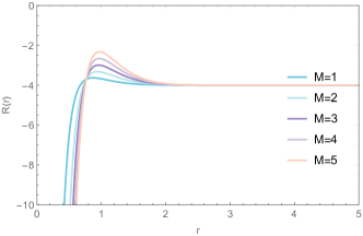
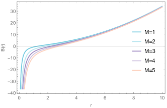
Figure 1: Plot of the curvature and the metric function for various values of $M$, while we have fixed $A=\sqrt{2}$ to have $c_{1}=2$ and $\Lambda_{\text{eff}}=-1$ .

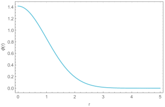
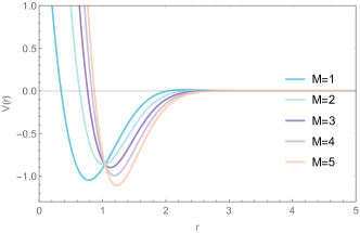
Figure 2: Plot of the scalar field and the potential for various values of $M$, while we have fixed $A=\sqrt{2}$ to have $c_{1}=2$ and $\Lambda_{\text{eff}}=-1$ .

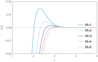
Figure 3: Plot of the potential outside the horizon for various values of $M$, while we have fixed $A=\sqrt{2}$ to have $c_{1}=2$ and $\Lambda_{\text{eff}}=-1$ .

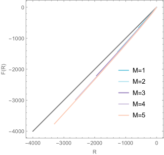
Figure 4: Compare the $F(R)$ functions with Einstein Gravity $F(R)=R$ (Gray line), while we have fixed $A=\sqrt{2}$ to have $c_{1}=2$ and $\Lambda_{\text{eff}}=-1$ .

For simplicity we rewrite the metric function as

$$B(r)=r^{2}\left[\int b(r)dr+c_{4}\right]~{},$$ (72)

where

$$b(r)=\frac{2r\left(A^{2}e^{-r^{2}}-8c_{1}-4c_{2}r\right)+\sqrt{\pi}A^{2}\left(2r^{2}+3\right)E(r)+8c_{3}}{2r^{4}\left(-A^{2}\left(\sqrt{\pi}rE(r)+2e^{-r^{2}}\right)+4c_{1}+4c_{2}r\right)}~{}.$$ (73)

Then

$$B^{\prime}(r) = \frac{B(r)}{r}+r^{2}b(r)~{},$$ (74)

$$B^{\prime\prime}(r) = \frac{2B(r)}{r^{2}}+4rb(r)+r^{2}b^{\prime}(r)~{},$$ (75)

$$B^{\prime\prime\prime}(r) = r^{2}b^{\prime\prime}(r)+6rb^{\prime}(r)+6b(r)~{},$$ (76)

$$...$$ (77)

and at the event horizon $r_{h}$ we have

$$B(r_{h}) = 0~{},$$ (78)

$$B^{\prime}(r_{h}) = r_{h}^{2}b(r_{h})~{},$$ (79)

$$B^{\prime\prime}(r_{h}) = 4r_{h}b(r_{h})+r_{h}^{2}b^{\prime}(r_{h})~{},$$ (80)

$$B^{\prime\prime\prime}(r_{h}) = r_{h}^{2}b^{\prime\prime}(r_{h})+6r_{h}b^{\prime}(r_{h})+6b(r_{h})~{},$$ (81)

$$...$$ (82)

For the potential $V(r)$ we have

$$V^{\prime}(r_{h}) = B^{\prime}(r_{h})\phi^{\prime}(r_{h})^{2}=r_{h}^{2}b(r_{h})\phi^{\prime}(r_{h})^{2}~{},$$ (83)

and also

$$f^{\prime}(r_{h})=b(r_{h})\left(r_{h}\left(r_{h}\left(f_{R}^{\prime\prime}(r_{h})+\phi^{\prime}(r_{h})^{2}\right)+2f_{R}^{\prime}(r_{h})\right)-12f_{R}(r_{h})\right)-r_{h}f_{R}(r_{h})\left(r_{h}b^{\prime\prime}(r_{h})+8b^{\prime}(r_{h})\right)~{}.$$ (84)

As can be seen from the expressions (69)-(71) around the horizon of the metric function $B(r)$, the potential $V(r)$ and the function $f(r)$, if the scalar field backreacts to the metric at small distances there is no any exact hairy black hole solution and a numerically hairy black hole solution is resulted from a metric function (72) which is not simple. This can be understood from the fact that at small distances the modified curvature of the $f(R)$ theory is so strong that it gives strongly coupled hairy black holes.

II.2 Other matter distributions

If we consider another matter distribution we expect to get a similar structure of the hairy black holes at large and small distances. This will depend on the behaviour of the scalar field at large and small distances. Choosing different matter distributions will affect the form of the $f(R)$ function which nevertheless it will always have extra curvature terms other than the Ricci scalar $R$. If for example we choose a a polynomial distribution like

$$\phi(r)=\frac{A}{(r+s)^{p}}~{},$$ (85)

we will get

$$f_{R}(r)=-\frac{A^{2}p(r+s)^{-2p}}{4p+2}+c_{1}+c_{2}r~{},$$ (86)

or an inverse trigonometric function distribution of the scalar field

$$\phi(r)=\frac{\pi}{2}-\arctan{r}~{},$$ (87)

we will get

$$f_{R}(r)=-\frac{1}{2}r\arctan{r}+c_{1}+c_{2}r~{}.$$ (88)

Therefore we expect that strong and weak curvature effects of the $f(R)$ function at small and large distances will give hairy black hole solutions.

III Non Minimal Coupling

In this section we will consider a scalar field non minimally coupled to gravity and we will look for hairy black holes. The strength of the coupling between the scalar field and gravity is denoted by the factor $1/12$ (the conformal coupling factor) and in the action we also consider a self interacting potential. The motivation for this study is to show that choosing various matter distributions we can have the formation of hairy black holes at small distances if the scalar field is not minimally coupled. We will see that the scalarization mechanism depends internally on the dynamics of the scalar field before and after the formation of the horizon of the black hole.

Consider the action

$$S=\int d^{4}x\sqrt{-g}\big{[}\cfrac{1}{2\kappa}\big{(}f(R)-2\Lambda\big{)}-\cfrac{1}{2}g^{\mu\nu}\partial_{\mu}\phi\partial_{\nu}\phi-\cfrac{1}{12}R\phi^{2}-V(\phi)\big{]}~{}.$$ (89)

Varying this action we get the same field equation (2) but with a different energy-momentum tensor

$$T_{\mu\nu}=\partial_{\mu}\phi\partial_{\nu}\phi-\cfrac{1}{2}g_{\mu\nu}g^{\alpha\beta}\partial_{\alpha}\phi\partial_{\beta}\phi+\cfrac{1}{6}\left(g_{\mu\nu}\Box-\nabla_{\mu}\nabla_{\nu}+G_{\mu\nu}\right)\phi^{2}-g_{\mu\nu}V(\phi)~{},$$ (90)

and a different Klein-Gordon equation

$$\Box\phi-\cfrac{1}{6}R\phi-V^{\prime}(\phi)=0~{}.$$ (91)

Using same metric ansatz (5) and setting $\kappa=1$, from the $\theta\theta$ and $tt$ components of the Einstein equations we get

$$\cfrac{f_{R}(r)\left(-3r^{2}B^{\prime\prime}(r)+6B(r)-6\right)+r\left(rB^{\prime}(r)-2B(r)\right)\left(\phi(r)\phi^{\prime}(r)-3f_{R}^{\prime}(r)\right)}{12r^{2}B(r)}=0~{},$$ (92)

while from the $tt$ and $rr$ components of the Einstein equations we get

$$\frac{1}{6}B(r)^{2}\left(3f_{R}^{\prime\prime}(r)-\phi(r)\phi^{\prime\prime}(r)+2\phi^{\prime}(r)^{2}\right)=0~{}.$$ (93)

The Klein-Gordon equation reads

$$\frac{\left(rB^{\prime}(r)+2B(r)\right)\phi^{\prime}(r)}{r}+\frac{\phi(r)\left(r^{2}B^{\prime\prime}(r)+4rB^{\prime}(r)+2B(r)-2\right)}{6r^{2}}+B(r)\phi^{\prime\prime}(r)-\frac{V^{\prime}(r)}{\phi^{\prime}(r)}=0~{}.$$ (94)

As in the previous section with a scalar field minimally coupled to gravity, we will consider various matter distributions and we will study their effect on a spherically symmetric metric. Then having the forms of the scalar field $\phi(r)$ we will solve for $f_{R}(r)$ from equation (93), then we will get $B(r)$ and $V(r)$ numerically from equations (92) and (94) respectively.

In this case, the equations are hard to be even asymptotically integrated in full generality. Thus we can not give a proof of continuity like we did in the previous section. But for the boundary conditions we give, the numerical results show that they are continuous, then an horizon is formed, and we indeed observe similar behaviors with the minimally coupled case.

III.1 $\phi(r)=\cfrac{m}{r+n}$

We first consider the form of the scalar field $\phi(r)=\cfrac{m}{r+n}$ where $m$ and $n$ are constants. Then we get

$$f_{R}=C_{1}+C_{2}r~{},$$ (95)

and the metric function $B(r)$, $V(r)$ can be obtained numerically as shown in Fig. 5 and Fig. 6.

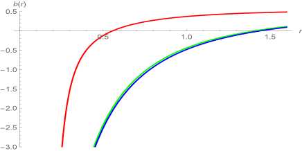
Figure 5: $B(r)$ for $m=C_{1}=C_{2}=1$, $n=1$ (Green), $n=0.01$ (Red), $n=-0.05$ (Blue).

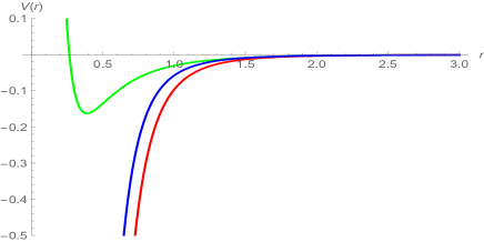
Figure 6: $V(r)$ for $m=C_{1}=C_{2}=1$, $n=1$ (Green), $n=0.01$ (Red), $n=-0.05$ (Blue).

The conditions we use here are: $B(0.2)=-10$, $B(100)=1$, $V(100)=0$. We can see that in the all cases with the conditions we give, there is an horizon formed and black hole solutions exist with a scalar field to behave well for all $r>0$ values.

For the $f(R)$ function we have from equation (95),

$$f^{\prime}(R) = C_{1}+C_{2}r(R)~{},$$ (96)

$$f(R) = C_{1}R+C_{2}\int^{R}r(R)dR~{},$$ (97)

where the parameter $C_{1}$ is dimensionless and $C_{2}$ have dimensions $\left[C_{2}\right]=L^{-1}$. Therefore if $C_{1}=1$ and $C_{2}\neq 0$ this solution can be considered as an extension of the Einstein gravity. The scalar charges play a role in determining the metric therefore the matter distribution will influence the form in the final $f(R)$ through the Ricci scalar.

III.2 $\phi(r)=me^{-nr}$

Next we consider the case of the scalar field to be $\phi(r)=me^{-nr}~{},$ where $m$ and $n$ are constants ($n>0$ for the appropriate asymptotic behaviour, with units $[L]^{-1}$). Then we get

$$f_{R}=-\frac{1}{12}m^{2}e^{-2nr}+C_{2}r+C_{1}~{},$$ (98)

and the metric function $B(r)$, $V(r)$ can be obtained numerically as shown in Fig. 7 and Fig. 8.

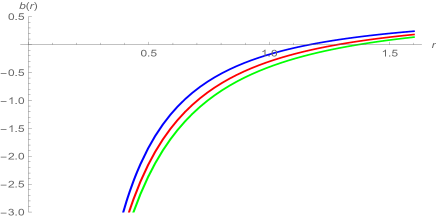
Figure 7: $B(r)$ for $m=C_{1}=C_{2}=1$, $n=1$ (Green), $n=1.5$ (Red), $n=2$ (Blue).

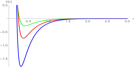
Figure 8: $V(r)$ for $m=C_{1}=C_{2}=1$, $n=1$ (Green), $n=1.5$ (Red), $n=2$ (Blue).

We can see that in all cases there is an horizon formed and black hole solutions exist with a scalar field to behave well for all $r>0$ values.

For the $f(R)$ function we can see from equation (98) that curvature corrections will be present in the final $f(R)$ form. The first term of equation (98) is related directly to the scalar field charges, while the last two terms will contain information about the scalar field indirectly through the metric function.

III.3 $\phi(r)=ArcTanh(\cfrac{m}{r+m}\big{)}$

Finally we consider the case of the scalar field to be

$$\phi(r)=ArcTanh(\cfrac{m}{r+m}\big{)}~{},$$

where $m$ is a constant with units $[L]$ and we get

$$f_{R}=\frac{(m+r)}{4m}\ln\big{(}\frac{r}{2m+r}\big{)}+\frac{1}{6}\tanh^{-1}\left(\frac{m}{m+r}\right)^{2}+C_{2}r+C_{1}~{},$$ (99)

and the functions $B(r)$, $V(r)$, $f_{R}$ and $\phi(r)$ can be obtained numerically as shown in Fig. 9-Fig. 12.

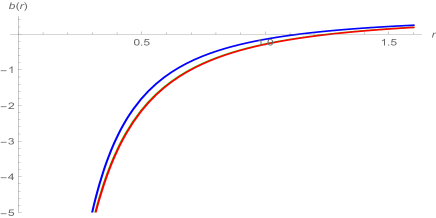
Figure 9: $B(r)$ for $C_{1}=C_{2}=1$,$m=1$ (Green), $m=0.05$ (Red), $m=5$ (Blue) (Green and Red are very close).

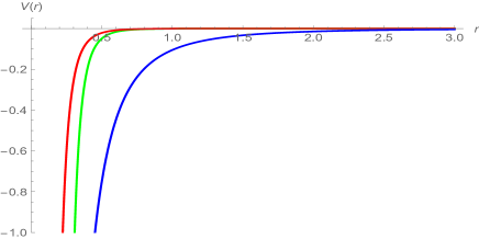
Figure 10: $V(r)$ for $C_{1}=C_{2}=1$, $m=1$ (Green), $m=0.05$ (Red), $m=5$ (Blue).

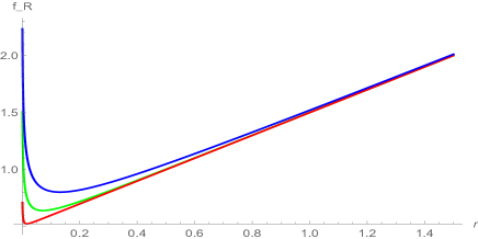
Figure 11: $f_{R}$ for $C_{1}=C_{2}=1$, $m=1$ (Green), $m=0.05$ (Red), $m=5$ (Blue).

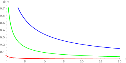
Figure 12: $\phi(r)$ for $C_{1}=C_{2}=1$, $m=1$ (Green), $m=0.05$ (Red), $m=5$ (Blue).

We can see that in all cases there is an horizon formed and black hole solutions exist with a scalar field to behave well for all $r>0$ values.

For the $f(R)$ function we can see from equation (99) that non-linear curvature corrections will appear in the final $f(R)$ form. These corrections are related directly to the scalar field charges due to equation (93) (the first two terms of equation (99)). Of course, the scalar field plays a role in the metric function $B(r)$ so it is expected that information about the scalar field will be present in the Ricci scalar and more non-linear corrections will finally appear because of the last two terms of equation (99), assuming of course that the Ricci scalar is dynamical.

We can see that in all the above cases, the scalar field modifies the gravitational model at hand, depending each time on the scalar field profile. The first polynomial distribution for example, seems to modify indirectly the gravitational model, while the other two distributions play a profound role in the final $f(R)$ model. The integration constants $C_{1}$ and $C_{2}$ have a physical meaning. $C_{1}$ is related to Einstein Gravity and $C_{2}$ is related to geometric corrections that can be encoded in $f(R)$ gravity, as it can be seen in equation (97). Also observe that in all cases the potential well is formed before the formation of the horizon of the black hole which agrees with our findings in the case of a scalar field minimally coupled to gravity.

IV Discussion and Conclusions

In this work we studied the production of scalarized black hole solutions in $f(R)$ gravity. Without specifying the form of the $f(R)$ function we introduced a scalar field minimally coupled to gravity. Solving the coupled field equations we showed that there are no any black hole solutions. Introducing a self-interacting scalar potential and considering a matter distribution backreacting on the metric we found that the Schwarzschild-AdS black hole is scalarized at large distances depending on particular choices of parameters. With a different choice of parameters scalarized Schwarzschild-AdS-like black holes can be found. The AdS space is generated by an effective cosmological constant which depends on the parameters.

At small distances we solved numerically the Einstein and Klein-Gordon equations. We found that the curvature is divergent at origin $r\rightarrow 0$ indicating a singularity and all the functions are continuous for any positive $r$. The metric function develops an event horizon while the scalar potential appears with a deep well which is formed before the formation of the event horizon and also develops a peak outside the event horizon. At small distances we find a similar behaviour of a scalar field conformally coupled to gravity. Considering various matter distributions we found that at small distances hairy black holes are produced and the scalar potential develops a deep well before the formation of the event horizon.

We attribute the scalarization of the black hole at large distances and the production of hairy black holes at small distances to pure curvature effects. This is a result of the solutions of the field equations which introduce non-linear curvature correction terms which appeared in the final $f(R)$ form. These correction terms are related directly to the scalar field charges of the considered matter distributions. At large distances these correction terms are weak and the usual Ricci scalar term dominates and the coupling of the scalar field to the metric scalarized the Schwarzschild-AdS or Schwarzschild-AdS-like black holes. At small distances the non-linear curvature correction terms dominate and then strong curvature and scalar dynamics give a rich structure of hairy black hole solutions. We expect that matter is trapped in the formed potential well and the scalar dynamics scalarized the black hole while after the formation of the hairy black hole it manifests itself with a peak of its potential outside the event horizon of the black hole. With a specific choice of parameters we found that the metric function exhibits a continuation from small to large distances connecting the solutions found in these regimes.

It would be very interesting to study in details the dynamical mechanism of how the matter trapped in the potential results to the formation of the hairy black hole. We have to stress here that the mechanism of the formation of hairy black hole is a result of the direct coupling of matter to gravity. There are other mechanisms of the formation of hairy black holes. On of them is the well known Gubser mechanism Gubser:2005ih on which the gauge/gravity holographic duality depends on it. A charged scalar field in the vicinity of a charged black hole in the AdS space is trapped outside the horizon of the black hole as a result of the competing forces of electromagnetic and gravitational forces. Another mechanism was discussed in Sotiriou:2014pfa ; Doneva:2017bvd ; Antoniou:2017acq and in its charged version Doneva:2018rou in which a black hole is scalarized because matter is coupled to the Gauss-Bonnet term, which is a high order curvature term. We note here that our mechanism is different from this mechanism because the scalar field is not directly coupled to curvature but it feels the strong curvature effect only through its coupling to the metric.

V Acknowledgements

We thank Ricardo Troncoso for his stimulating comments and suggestions.

References

-
(1)
N. Bocharova, K. Bronnikov and V. Melnikov, Vestn. Mosk.
Univ. Fiz. Astron. 6, 706 (1970);
J. D. Bekenstein, Annals Phys. 82, 535 (1974);
J. D. Bekenstein, “Black Holes With Scalar Charge,” Annals Phys. 91, 75 (1975). - (2) K. A. Bronnikov and Y. N. Kireyev, “Instability of black holes with scalar charge,” Phys. Lett. A 67, 95 (1978).
- (3) C. Martinez and J. Zanelli, “Conformally dressed black hole in (2+1)-dimensions,” Phys. Rev. D 54, 3830-3833 (1996) [arXiv:gr-qc/9604021 [gr-qc]].
- (4) M. Banados, C. Teitelboim and J. Zanelli, “The Black hole in three-dimensional space-time,” Phys. Rev. Lett. 69, 1849-1851 (1992) [arXiv:hep-th/9204099 [hep-th]].
- (5) C. Martinez, R. Troncoso and J. Zanelli, “Exact black hole solution with a minimally coupled scalar field,” Phys. Rev. D 70, 084035 (2004) [arXiv:hep-th/0406111 [hep-th]].
- (6) K. G. Zloshchastiev, “On co-existence of black holes and scalar field,” Phys. Rev. Lett. 94, 121101 (2005) [arXiv:hep-th/0408163].
- (7) C. Martinez, R. Troncoso and J. Zanelli, “De Sitter black hole with a conformally coupled scalar field in four-dimensions,” Phys. Rev. D 67, 024008 (2003) [hep-th/0205319].
- (8) G. Dotti, R. J. Gleiser and C. Martinez, “Static black hole solutions with a self interacting conformally coupled scalar field,” Phys. Rev. D 77, 104035 (2008) [arXiv:0710.1735 [hep-th]].
- (9) T. Torii, K. Maeda and M. Narita, “Scalar hair on the black hole in asymptotically anti-de Sitter spacetime,” Phys. Rev. D 64, 044007 (2001).
- (10) E. Winstanley, “On the existence of conformally coupled scalar field hair for black holes in (anti-)de Sitter space,” Found. Phys. 33, 111 (2003) [arXiv:gr-qc/0205092].
- (11) C. Martinez, J. P. Staforelli and R. Troncoso, “Topological black holes dressed with a conformally coupled scalar field and electric charge,” Phys. Rev. D 74, 044028 (2006) [arXiv:hep-th/0512022];
- (12) G. Koutsoumbas, S. Musiri, E. Papantonopoulos and G. Siopsis, “Quasi-normal Modes of Electromagnetic Perturbations of Four-Dimensional Topological Black Holes with Scalar Hair,” JHEP 0610, 006 (2006) [hep-th/0606096].
- (13) C. Martinez and A. Montecinos, “Phase transitions in charged topological black holes dressed with a scalar hair,” Phys. Rev. D 82 (2010) 127501 [arXiv:1009.5681 [hep-th]].
- (14) C. Martinez and R. Troncoso, “Electrically charged black hole with scalar hair,” Phys. Rev. D 74, 064007 (2006) [arXiv:hep-th/0606130].
- (15) T. Kolyvaris, G. Koutsoumbas, E. Papantonopoulos and G. Siopsis, “A New Class of Exact Hairy Black Hole Solutions,” Gen. Rel. Grav. 43, 163-180 (2011) [arXiv:0911.1711 [hep-th]].
- (16) C. Charmousis, T. Kolyvaris and E. Papantonopoulos, “Charged C-metric with conformally coupled scalar field,” Class. Quant. Grav. 26, 175012 (2009) [arXiv:0906.5568 [gr-qc]].
- (17) A. Anabalon, “Exact Black Holes and Universality in the Backreaction of non-linear Sigma Models with a potential in (A)dS4,” JHEP 1206, 127 (2012) [arXiv:1204.2720 [hep-th]].
- (18) A. Anabalon and J. Oliva, “Exact Hairy Black Holes and their Modification to the Universal Law of Gravitation,” Phys. Rev. D 86, 107501 (2012) [arXiv:1205.6012 [gr-qc]].
- (19) A. Anabalon and A. Cisterna, “Asymptotically (anti) de Sitter Black Holes and Wormholes with a Self Interacting Scalar Field in Four Dimensions,” Phys. Rev. D 85, 084035 (2012) [arXiv:1201.2008 [hep-th]].
- (20) Y. Bardoux, M. M. Caldarelli and C. Charmousis, “Conformally coupled scalar black holes admit a flat horizon due to axionic charge,” JHEP 1209, 008 (2012) [arXiv:1205.4025 [hep-th]].
- (21) P. A. González, E. Papantonopoulos, J. Saavedra and Y. Vásquez, “Four-Dimensional Asymptotically AdS Black Holes with Scalar Hair,” JHEP 12, 021 (2013) [arXiv:1309.2161 [gr-qc]].
- (22) A. Anabalon, D. Astefanesei and R. Mann, “Exact asymptotically flat charged hairy black holes with a dilaton potential,” JHEP 1310, 184 (2013) [arXiv:1308.1693 [hep-th]].
- (23) A. Anabalo’n and D. Astefanesei, “On attractor mechanism of black holes,” Phys. Lett. B 727, 568 (2013) [arXiv:1309.5863 [hep-th]].
- (24) P. A. González, E. Papantonopoulos, J. Saavedra and Y. Vásquez, “Extremal Hairy Black Holes,” JHEP 11, 011 (2014) [arXiv:1408.7009 [gr-qc]].
- (25) C. Charmousis, T. Kolyvaris, E. Papantonopoulos and M. Tsoukalas, “Black Holes in Bi-scalar Extensions of Horndeski Theories,” JHEP 1407, 085 (2014) [arXiv:1404.1024 [gr-qc]].
- (26) O. J. C. Dias, G. T. Horowitz and J. E. Santos, “Black holes with only one Killing field,” JHEP 1107, 115 (2011) [arXiv:1105.4167 [hep-th]].
- (27) S. Stotyn, M. Park, P. McGrath and R. B. Mann, “Black Holes and Boson Stars with One Killing Field in Arbitrary Odd Dimensions,” Phys. Rev. D 85, 044036 (2012) [arXiv:1110.2223 [hep-th]].
- (28) O. J. C. Dias, P. Figueras, S. Minwalla, P. Mitra, R. Monteiro and J. E. Santos, “Hairy black holes and solitons in global ,” JHEP 1208, 117 (2012) [arXiv:1112.4447 [hep-th]].
- (29) B. Kleihaus, J. Kunz, E. Radu and B. Subagyo, “Axially symmetric static scalar solitons and black holes with scalar hair,” Phys. Lett. B 725, 489 (2013) [arXiv:1306.4616 [gr-qc]].
- (30) H. Lu, C. Pope and Q. Wen, “Thermodynamics of AdS Black Holes in Einstein-Scalar Gravity,” JHEP 03, 165 (2015) [arXiv:1408.1514 [hep-th]].
- (31) G. Koutsoumbas, K. Ntrekis, E. Papantonopoulos and M. Tsoukalas, “Gravitational Collapse of a Homogeneous Scalar Field Coupled Kinematically to Einstein Tensor,” Phys. Rev. D 95, no.4, 044009 (2017) [arXiv:1512.05934 [gr-qc]].
- (32) T. Kolyvaris, G. Koutsoumbas, E. Papantonopoulos and G. Siopsis, “Scalar Hair from a Derivative Coupling of a Scalar Field to the Einstein Tensor,” Class. Quant. Grav. 29, 205011 (2012) [arXiv:1111.0263 [gr-qc]].
- (33) T. Kolyvaris, G. Koutsoumbas, E. Papantonopoulos and G. Siopsis, “Phase Transition to a Hairy Black Hole in Asymptotically Flat Spacetime,” JHEP 1311, 133 (2013) [arXiv:1308.5280 [hep-th]].
- (34) M. Rinaldi, “Black holes with non-minimal derivative coupling,” Phys. Rev. D 86, 084048 (2012) [arXiv:1208.0103 [gr-qc]].
- (35) E. Babichev and C. Charmousis, “Dressing a black hole with a time-dependent Galileon,” JHEP 1408, 106 (2014) [arXiv:1312.3204 [gr-qc]].
- (36) S. W. Hawking, M. J. Perry and A. Strominger, “Soft Hair on Black Holes,” Phys. Rev. Lett. 116, no.23, 231301 (2016) [arXiv:1601.00921 [hep-th]].
- (37) H. Afshar, S. Detournay, D. Grumiller, W. Merbis, A. Perez, D. Tempo and R. Troncoso, “Soft Heisenberg hair on black holes in three dimensions,” Phys. Rev. D 93, no.10, 101503 (2016) [arXiv:1603.04824 [hep-th]].
- (38) D. Grumiller, A. Pérez, M. M. Sheikh-Jabbari, R. Troncoso and C. Zwikel, “Spacetime structure near generic horizons and soft hair,” Phys. Rev. Lett. 124, no.4, 041601 (2020) [arXiv:1908.09833 [hep-th]].
- (39) A. De Felice and S. Tsujikawa, “f(R) theories,” Living Rev. Rel. 13, 3 (2010), [arXiv:1002.4928 [gr-qc]].
- (40) G. Cognola, E. Elizalde, S. Nojiri, S. D. Odintsov, L. Sebastiani and S. Zerbini, “A Class of viable modified f(R) gravities describing inflation and the onset of accelerated expansion,” Phys. Rev. D 77 (2008) 046009 [arXiv:0712.4017 [hep-th]].
- (41) L. Pogosian and A. Silvestri, “The pattern of growth in viable f(R) cosmologies,” Phys. Rev. D 77 (2008) 023503 Erratum: [Phys. Rev. D 81 (2010) 049901] [arXiv:0709.0296 [astro-ph]].
- (42) P. Zhang, “Testing gravity against the large scale structure of the universe.,” Phys. Rev. D 73 (2006) 123504 [astro-ph/0511218].
- (43) B. Li and J. D. Barrow, “The Cosmology of f(R) gravity in metric variational approach,” Phys. Rev. D 75 (2007) 084010 [gr-qc/0701111].
- (44) Y. S. Song, H. Peiris and W. Hu, “Cosmological Constraints on f(R) Acceleration Models,” Phys. Rev. D 76 (2007) 063517 [arXiv:0706.2399 [astro-ph]].
- (45) S. Nojiri and S. D. Odintsov, “Modified f(R) gravity unifying R**m inflation with Lambda CDM epoch,” Phys. Rev. D 77 (2008) 026007 [arXiv:0710.1738 [hep-th]].
- (46) S. Nojiri and S. D. Odintsov, “Unifying inflation with LambdaCDM epoch in modified f(R) gravity consistent with Solar System tests,” Phys. Lett. B 657 (2007) 238 [arXiv:0707.1941 [hep-th]].
- (47) S. Capozziello, C. A. Mantica and L. G. Molinari, “Cosmological perfect-fluids in f(R) gravity,” Int. J. Geom. Meth. Mod. Phys. 16 (2018) no.01, 1950008 [arXiv:1810.03204 [gr-qc]].
- (48) A. A. Starobinsky, “A New Type of Isotropic Cosmological Models Without Singularity,” Phys. Lett. B 91 (1980) 99 [Phys. Lett. 91B (1980) 99] [Adv. Ser. Astrophys. Cosmol. 3 (1987) 130].
- (49) M. Ostrogradsky, “Mémoires sur les équations différentielles, relatives au problème des isopérimètres,” Mem. Acad. St. Petersbourg 6 (1850) no.4, 385.
- (50) R. P. Woodard, “Avoiding dark energy with 1/r modifications of gravity,” Lect. Notes Phys. 720 (2007) 403 [astro-ph/0601672].
- (51) T. Multamaki and I. Vilja, “Spherically symmetric solutions of modified field equations in f(R) theories of gravity,” Phys. Rev. D 74 (2006) 064022 [astro-ph/0606373].
- (52) T. Multamaki and I. Vilja, “Static spherically symmetric perfect fluid solutions in f(R) theories of gravity,” Phys. Rev. D 76 (2007) 064021 [astro-ph/0612775].
- (53) A. de la Cruz-Dombriz, A. Dobado and A. L. Maroto, “Black Holes in f(R) theories,” Phys. Rev. D 80 (2009) 124011 Erratum: [Phys. Rev. D 83 (2011) 029903] [arXiv:0907.3872 [gr-qc]].
- (54) S. H. Hendi, B. Eslam Panah and S. M. Mousavi, “Some exact solutions of F(R) gravity with charged (a)dS black hole interpretation,” Gen. Rel. Grav. 44, 835 (2012) [arXiv:1102.0089 [hep-th]].
- (55) L. Sebastiani and S. Zerbini, “Static Spherically Symmetric Solutions in F(R) Gravity,” Eur. Phys. J. C 71 (2011) 1591 [arXiv:1012.5230 [gr-qc]].
- (56) L. Hollenstein and F. S. N. Lobo, “Exact solutions of f(R) gravity coupled to nonlinear electrodynamics,” Phys. Rev. D 78 (2008) 124007 [arXiv:0807.2325 [gr-qc]].
- (57) S. Capozziello, M. De laurentis and A. Stabile, “Axially symmetric solutions in f(R)-gravity,” Class. Quant. Grav. 27 (2010) 165008 [arXiv:0912.5286 [gr-qc]].
- (58) T. Moon, Y. S. Myung and E. J. Son, “f(R) black holes,” Gen. Rel. Grav. 43 (2011) 3079 [arXiv:1101.1153 [gr-qc]].
- (59) J. A. R. Cembranos, A. de la Cruz-Dombriz and P. Jimeno Romero, “Kerr-Newman black holes in theories,” Int. J. Geom. Meth. Mod. Phys. 11 (2014) 1450001 [arXiv:1109.4519 [gr-qc]].
- (60) E. Hernandéz-Lorenzo and C. F. Steinwachs, “Naked singularities in quadratic gravity,” Phys. Rev. D 101, no.12, 124046 (2020) [arXiv:2003.12109 [gr-qc]].
- (61) S. Soroushfar, R. Saffari and N. Kamvar, “Thermodynamic geometry of black holes in f(R) gravity,” Eur. Phys. J. C 76 (2016) no.9, 476 [arXiv:1605.00767 [gr-qc]].
- (62) G. G. L. Nashed and S. Capozziello, “Charged spherically symmetric black holes in gravity and their stability analysis,” Phys. Rev. D 99, no. 10, 104018 (2019) [arXiv:1902.06783 [gr-qc]].
- (63) Z. Y. Tang, B. Wang and E. Papantonopoulos, “Exact charged black hole solutions in D-dimensions in f(R) gravity,” [arXiv:1911.06988 [gr-qc]].
- (64) A. Aragón, P. A. González, E. Papantonopoulos and Y. Vásquez, “Quasinormal modes and their anomalous behavior for black holes in gravity,” [arXiv:2005.11179 [gr-qc]].
- (65) S. S. Gubser, “Phase transitions near black hole horizons,” Class. Quant. Grav. 22, 5121-5144 (2005) [arXiv:hep-th/0505189 [hep-th]].
- (66) T. P. Sotiriou and S. Y. Zhou, “Black hole hair in generalized scalar-tensor gravity: An explicit example,” Phys. Rev. D 90, 124063 (2014) [arXiv:1408.1698 [gr-qc]].
- (67) D. D. Doneva and S. S. Yazadjiev, “New Gauss-Bonnet Black Holes with Curvature-Induced Scalarization in Extended Scalar-Tensor Theories,” Phys. Rev. Lett. 120, no.13, 131103 (2018) [arXiv:1711.01187 [gr-qc]].
- (68) G. Antoniou, A. Bakopoulos and P. Kanti, “Evasion of No-Hair Theorems and Novel Black-Hole Solutions in Gauss-Bonnet Theories,” Phys. Rev. Lett. 120, no.13, 131102 (2018) [arXiv:1711.03390 [hep-th]].
- (69) D. D. Doneva, S. Kiorpelidi, P. G. Nedkova, E. Papantonopoulos and S. S. Yazadjiev, “Charged Gauss-Bonnet black holes with curvature induced scalarization in the extended scalar-tensor theories,” Phys. Rev. D 98, no.10, 104056 (2018) [arXiv:1809.00844 [gr-qc]].