Preference robust optimization with quasi-concave choice functions for multi-attribute prospects

Abstract

Preference robust choice models concern decision-making problems where the decision maker’s (DM) utility/risk preferences are ambiguous and the evaluation is based on the worst-case utility function/risk measure from a set of plausible utility functions/risk measures. The current preference robust choice models are mostly built upon von Neumann-Morgenstern expected utility theory, the theory of convex risk measures, or Yaari’s dual theory of choice, all of which assume the DM’s preferences satisfy some specified axioms. In this paper, we extend the preference robust approach to a broader class of choice functions which satisfy monotonicity and quasi-concavity in the space of multi-attribute random prospects. While our new model is non-parametric and significantly extends the coverage of decision-making problems, it also brings new computational challenges due to the non-convexity of the optimization formulations, which arises from the non-concavity of the class of quasi-concave choice functions. To tackle these challenges, we develop a sorting-based algorithm that efficiently evaluates the robust choice function (RCF) by solving a sequence of linear programming problems. Then, we show how to solve preference robust optimization (PRO) problems by solving a sequence of convex optimization problems. We test our robust choice model and computational scheme on a single-attribute portfolio optimization problem and a multi-attribute capital allocation problem.

Key words: preference robust optimization, quasi-concave choice functions, multi-attribute choice models

1 Introduction

Much of the focus of the literature on decision-making under uncertainty has been on exogenous uncertainties such as market returns, customer demand, traffic flow, and weather conditions. In some problems, there is also substantial endogenous uncertainty about the decision maker’s (DM’s) own preferences that we refer to as preference ambiguity. Such ambiguity may arise due to the DM’s inability to precisely articulate its own preferences, a lack of accurate models for human behavior, or scarce observations of the DM’s past choices. In behavioural economics, the DM’s preferences are characterized by a choice function where one random prospect is preferred to another if and only if the choice function value of the former is larger than that of the latter. Expected utility (Von Neumann and Morgenstern, 1945) (VNM), convex risk measures (Artzner et al., 1999), and Yaari’s dual theory of choice (Yaari, 1987) are all well known specific families of choice functions. The properties of the choice function match the structure of the DM’s preferences, and different families of choice functions correspond to different types of DMs. When information on the DM’s preferences is incomplete, the choice function used to characterize these preferences is ambiguous.

In this case we cannot provide an optimization problem for the DM that best reflects their preferences. Since the optimal decision is highly sensitive to the DM’s preferences, we are at risk of misspecifying the description of the DM’s preferences and arriving at a greatly sub-optimal solution. The preference robust optimization (PRO) paradigm is first developed in (Armbruster and Delage, 2015) to deal with this situation. In PRO, we use available partial information on the DM to construct an ambiguity set of possible choice functions. This information can include structural assumptions (e.g., monotonicity or concavity) and other auxiliary information about the DM (e.g., preference elicitation information from pairwise comparisons). Then, to mitigate the preference ambiguity, the optimal decision is based on the worst-case choice function from this ambiguity set.

Several PRO models have been considered for various types of DMs (corresponding to different families of choice functions). Armbruster and Delage (2015) and the follow-up utility-based PRO models (e.g., Delage et al. (2017)) presume the DM’s preferences are characterized by VNM-type expected utility. Alternatively, the PRO models in Delage and Li (2017), Li (2021) are based on DMs whose preferences are characterized by convex risk measures. The PRO models in Guo and Xu (2021), Wang and Xu (2020) are designed for DMs whose preferences are characterized by Yaari’s dual theory of choice.

In this paper, we build a new PRO model to support a wider range of DMs and their preferences. First, our new PRO model emphasizes quasi-concave choice functions to incorporate diversification-favoring preferences in the broadest possible way (while previous PRO models emphasize concavity/convexity to reflect diversification-favoring preferences). Second, our new PRO model naturally supports multi-attribute prospects (while previous PRO models largely emphasize the single-attribute case). Despite its greater generality, our model can still be applied efficiently to large-scale problems.

1.1 Motivating examples

We motivate our present work by discussing two multi-attribute decision-making problems. We also elaborate on the kinds of partial information we can elicit from the DM, even when their exact preferences are ambiguous.

Example 1.1 (Investment).

Consider a company which plans to invest in Europe. The company evaluates an investment based on three (possibly random) factors: market environment ($X_{1}$), profitability ($X_{2}$), and market share ($X_{3}$). The company’s overall evaluation of an investment may be described by a choice function $\phi$ on random vectors $X=(X_{1},X_{2},X_{3})$, where $\phi(X)$ is the company’s evaluation of a particular investment.

The company’s choice function captures the effects of each factor as well as their interacting effects on the overall evaluation of an investment. However, we cannot identify a unique choice function when there is incomplete information about the company’s preferences. Yet, we can still elicit some basic properties of the choice function $\phi$. One is monotonicity, that is, a better market environment (e.g., less competitive, better regulated), and/or higher profitability, and/or a larger market share would all lead to higher values of $\phi$. The other property is quasi-concavity. For two investment opportunities $X^{1}=(X_{1}^{1},X_{2}^{1},X_{3}^{1})$ and $X^{2}=(X_{1}^{2},X_{2}^{2},X_{3}^{2})$, each of which has an evaluation equal to or exceeding some level $\alpha$, their convex combination will also give an overall evaluation of at least $\alpha$. This property corresponds to diversification-favouring behavior in the risk management literature (Simon, 1955, Brown and Sim, 2009, Brown et al., 2012).

These two properties restrict the company’s choice function to belong to a specific class (monotone and quasi-concave functions). It is possible to further narrow down the scope of possible choice functions with some questionnaires for the company. For example, we can pose pairs of alternative investments with different levels of the three factors and ask which one is preferred by the company. It is even possible to pose these questionnaires to all senior managers, and then synthesize the most conservative estimate of the group’s preferences. We refer to Armbruster and Delage (2015), Hu and Mehrotra (2015), Delage and Li (2017) for further discussion on pairwise preference elicitation.

Example 1.2 (Consumer preference).

Consumer preferences for mobile phones are determined by multiple features including price, storage capacity, water resistance, chip, battery, camera, video recording, software, and customer service. Although some of these features are deterministic upon purchase (e.g., price), many of them represent uncertainty due to fluctuation in actual performance from the specified standard (e.g., battery capacity), or the customer’s inability to quantify the attributes beforehand (e.g., quality of customer service). Let $X=(X_{1},\ldots,X_{9})$ denote the customer’s level of appreciation of the nine features of a mobile. We suppose $X_{i}=z_{i}+\xi_{i}$ where $z_{i}$ is the mean value of attribute $i$ and $\xi_{i}$ is random error which represents fluctuations in a particular customer’s actual experience. We let $\phi$ denote the customer’s choice function and $\phi(X)$ denote the corresponding choice function evaluation.

If we enhance one or more of the features, e.g., by reducing the price, increasing the capacity, or improving the service, then it will increase the overall evaluation of the product. This property corresponds to monotonicity of the choice function. For any two other mobiles $X^{1}$ and $X^{2}$ for which the consumer’s overall evaluation exceeds $\alpha$, we believe that any convex combination $X_{\lambda}=\lambda\,X^{1}+(1-\lambda)X^{2}$ for $\lambda\in(0,1)$ will also give the consumer an overall evaluation of at least $\alpha$. In other words, if the consumer is satisfied with both $X^{1}$ and $X^{2}$, then he/she should also be satisfied with any convex combination of them. This property corresponds to quasi-concavity of the choice function.

Suppose the customer’s preferences can be represented by the quasi-concave choice function

$$\phi(X)=u^{-1}(\mathbb{E}[u(\langle w,\,X\rangle)]),$$

where $w=(w_{1},\ldots,w_{9})$ denotes the customer’s weights on the attributes and $u$ is a piecewise function defined by:

$$u(x)=\begin{cases}3-\exp(-\gamma\left(x-2\right)),&x\geq 2,\\ \gamma(x-2)+2,&x<2,\end{cases}$$

with $\gamma=0.1$. We take the particular weights given in the following table.

$w_{1}$	$w_{2}$	$w_{3}$	$w_{4}$	$w_{5}$	$w_{6}$	$w_{7}$	$w_{8}$	$w_{9}$
0.1837	0.1668	0.0645	0.0124	0.0071	0.1737	0.1240	0.0442	0.2235

The weights can be obtained via surveys or decision analysis tools like Analytic Hierarchy Processes or Analytic Network Processes. In practice we do not know the true choice function, so we might then use expected power utility to describe the customer’s preference s

$$U(X)=\mathbb{E}[(\langle w,\,X\rangle)^{\beta}],$$

where $\beta\in[0,\,1]$ is a parameter.

Suppose we estimate $\beta=0.821$ via logistic approach (see e.g. Lopez-Guzman et al. (2018)). With these specific parameter values, we can compare $\phi(X)$ and $U(X)$ for a specific mobile $X$ to obtain:

	Mobile 1	Mobile 2
$\phi$	1.980	1.970
$U$	1.723	1.724

We see that a naive parametric expected utility function cannot make the right prediction about the customer’s preferences when they can only be represented by a quasi-concave choice function.

In both of these examples, the DM’s preferences are ambiguous but we still have some partial information. We build a robust choice model that uses this partial information to compute the most conservative estimate of the DM’s preferences, which can then be used in subsequent optimization problems.

1.2 Contributions

As our main contribution, we create a robust choice model for preference ambiguity where the underlying choice function is monotone, quasi-concave, and (possibly) multi-attribute. Many of the existing PRO models represent diversification-favoring behavior through the stronger properties of concavity (for utility) or convexity (for monetary risk measures). However, these properties do not capture all forms of diversification-favoring behavior. In full generality, diversification-favoring behavior means that if two prospects are acceptable at some level, then any mixture should also be acceptable at this same level. For translation-invariant monetary risk measures, diversification-favoring behavior implies convexity. However, as argued by Cerreia-Vioglio et al. (2011), it only leads to quasi-convexity if the DM’s choice function is not translation invariant (see El Karoui and Ravanelli (2009) for reasons why translation invariance fails).

As a specific example of the importance of quasi-concavity, it has been shown that VNM expected utility theory cannot be used to effectively describe some economic behaviours (see Allais (1953), Kahneman and Tversky (2013)). The Allais Paradox (Allais, 1953) demonstrates that a DM’s preferences can be inconsistent with expected utility theory for “any” utility function. Brown et al. (2012) show that the Allais Paradox can be resolved with a class of quasi-concave choice functions called aspirational measures. Quasi-concavity is the key structural property that enables us to represent diversification-favoring preferences in the most general way, and to do PRO for the entire class of diversification-favoring DM’s.

Our robust choice model is encapsulated by a robust choice function (RCF) which gives the most conservative estimate of the DM’s preferences based on available partial information. Our first task is to evaluate the RCF with an appropriate optimization formulation. We do this by identifying the class of majorants of quasi-concave choice functions, and then using them to enforce the property of quasi-concavity as a constraint in our optimization formulation. As a consequence of the property of quasi-concavity (which is not preserved by convex combination), this formulation is non-convex. Yet, we can exploit special problem structure to solve it efficiently with a two-stage approach. The first stage “value problem” determines the value of the RCF on a set of distinguished prospects and the second stage “interpolation problem” evaluates a new prospect based on these values. We propose a novel sorting algorithm to efficiently solve the non-convex value problem based on a sequence of LPs. The optimal solution of the value problem can then be taken as input to the simpler and less expensive interpolation problem to evaluate prospects as needed. We can also incorporate the property of law invariance into this procedure. While law invariance introduces exponentially many variables and constraints into our optimization formulations, we can reduce both of these to only a polynomial number and still solve these problems efficiently.

Next, we do PRO by optimizing the RCF (for both the base and law invariant cases). The acceptance sets of the RCF follow from the solution of the value problem and can be characterized explicitly. In particular, we show that they are all polyhedra. We can then efficiently optimize the RCF by doing binary search over its levels, where at each level we solve a convex optimization problem to check membership of the corresponding acceptance set. This method only requires us to solve a logarithmic number of convex optimization problems.

Our robust choice model supports multi-attribute problems, which are ubiquitous. For instance, several metrics are used in healthcare to measure the quality of life (Feeny et al., 2002, Smith and Keeney, 2005). Multi-attribute problems are also found in product design (Kim and Chhajed, 2002), auction mechanism design (Beil and Wein, 2003, Parkes and Kalagnanam, 2005, Chen-Ritzo et al., 2005), and competitive positioning of business strategy (Adner et al., 2014). Indeed, over the past few decades, there has been significant research on multi-attribute expected utility (Von Stengel, 1988, Fishburn and LaValle, 1992, Miyamoto and Wakker, 1996, Tsetlin and Winkler, 2006, 2007, 2009) and multi-attribute risk management (Jouini et al., 2004, Burgert and Rüschendorf, 2006, Hamel and Heyde, 2010, Galichon and Henry, 2012). The existing PRO models emphasize single-attribute problems, and their formulations do not directly extend to the multi-attribute case. However, our model supports the multi-attribute case without any modification. In our capital allocation problem, we demonstrate that our sorting algorithm for constructing the RCF (both with and without law invariance) has strong scalability in terms of the number of attributes. Similarly, the complexity of our binary search algorithm for optimizing the RCF also grows slowly in the number of attributes.

1.3 Literature review

1.3.1 Utility-based PRO models

There are two ingredients in VNM expected utility theory: (i) the utility function represents the DM’s risk attitudes and tastes; and (ii) the probability distribution represents the DM’s beliefs about the underlying uncertainty on the states of the world. Classical VNM expected utility theory assumes there is no ambiguity in either of these ingredients, while an important stream of research focuses on ambiguity in the DM’s tastes. Such ambiguity may arise from a lack of an accurate description of human behaviour (Thurstone (1927)), cognitive difficulty, or incomplete information (Karmarkar (1978) and Weber (1987)). Parametric and non-parametric approaches have been proposed to estimate the true utility function, these include discrete choice models (Train, 2009), standard and paired gambling approaches for preference comparisons, and certainty equivalence (Farquhar, 1984). We refer readers to Hu et al. (2018) for an overview of the utility estimation approach.

In decision-making under uncertainty, the DM may mitigate the overall risk by choosing the worst-case utility function among a set of plausible utility functions representing his/her risk preferences. This approach can be traced back to Maccheroni (2002). Armbruster and Delage (2015) give a comprehensive treatment of this topic from the perspective of minimax preference robust optimization (PRO). Specifically, they construct an ambiguity set that combines structural properties of utility functions such as monotonicity, concavity, and S-shapedness, along with user-specific preference information elicited through pairwise comparison questionnaires. They derive tractable reformulations for the resulting PRO problem by exploiting the affine majorants of the class of concave functions (which characterize the property of concavity) to obtain convex optimization problems.

Hu and Mehrotra (2015) also do PRO for VNM-type DMs, but they construct the ambiguity set differently. They establish an equivalence between increasing convex utility functions and CDFs. Then, they construct a moment-type ambiguity set for the DM’s utility function based on the certainty equivalent, pairwise comparisons, upper and lower bounds of the trajectories of the utility functions, and bounds on their derivatives. They derive a tractable LP reformulation of their resulting PRO problem based on a piecewise linear approximation.

Delage et al. (2017) propose a robust choice model for investors whose preferences are expressed by a shortfall risk measure and who are ambiguous about their utility loss function. They construct an ambiguity set for the utility loss function that can accommodate convexity, boundedness, coherence, and pairwise comparisons. Then, they obtain a tractable LP reformulation of their PRO problem. This model is extended by Zhang et al. (2020) to multivariate shortfall risk measures and by Zhang and Xu (2021b) to generalized shortfall risk measures based on cumulative prospect theory.

The problem of ambiguity in the DM’s tastes is also related to cautious expected utility (Cerreia-Vioglio et al., 2015) which considers the worst-case certainty equivalent from a given set of utility functions. Cerreia-Vioglio et al. (2015) show that the DM’s risk preferences can be represented by a worst-case certainty equivalent if and only if they are given by a binary relation satisfying the weak order, continuity, weak monotonicity, and negative certainty independence (NCI). We also point out the connection between utility-based PRO and optimization with stochastic dominance constraints (see, e.g., Dentcheva and Ruszczyński (2004)). Stochastic dominance constraints require all DM’s with utility functions in a certain class to prefer a candidate prospect to a benchmark.

1.3.2 Other PRO models

Delage and Li (2017), Li (2021) do PRO for the class of convex risk measures. They construct an ambiguity set of risk measures based on properties such as convexity, coherence, law invariance, and elicited preferences. They then develop tractable reformulations using the acceptance set representation for convex risk measures, which allows their PRO models to be solved with linear programming and convex optimization. Li (2021) further incorporates inverse optimization information into the construction of the ambiguity set by observing the DM’s past optimal decisions. The optimization formulations in Delage and Li (2017), Li (2021) are also based on the special properties of affine majorants/minorants of concave/convex functions (this special property is used earlier in Armbruster and Delage (2015) as well).

Wang and Xu (2020) consider preference ambiguity in spectral risk measures (SRM), which are based on Yaari’s dual theory of choice. They introduce a robust SRM model based on the worst-case risk spectrum from a ball centred at a nominal risk spectrum. A step-like approximation for the risk spectra is developed and used in optimization to get a tractable problem, and an error bound for the approximation is derived.

There is other work on robust multi-attribute choice models, for instance see Lam et al. (2013), Ehrgott et al. (2014). Noyan and Rudolf (2018) consider multi-attribute PRO for a general class of scalarization functions (i.e., the class of min-biaffine functions), where the vector of weights for the multiple attributes lies in a convex ambiguity set. Vayanos et al. (2020) study active preference elicitation for multi-attribute problems, under both the max-min utility and min-max regret decision criteria. They focus on the trade-offs between the multiple attributes, and show that their problem can be formulated as a two-stage (resp. multi-stage) robust optimization problem with decision-dependent information discovery and solved efficiently.

1.3.3 Quasi-concavity

Quasi-concave choice functions have already appeared widely in the literature. One of the most prevalent examples of a quasi-concave choice function is the certainty equivalent (see, e.g., Ben-Tal and Teboulle (2007)). The indices of acceptability proposed by Cherny and Madan (2009) are also quasi-concave choice functions.

Brown and Sim (2009) develop the class of satisficing measures, which are based on the idea of meeting a target (satisficing rather than optimizing), and which are quasi-concave. Their work is continued in Brown et al. (2012) where the authors develop the class of aspirational measures. This class of measures is allowed to be quasi-concave on a diversification-favoring set, and quasi-convex on a concentration-favoring set. The representation result in Brown et al. (2012) shows that aspirational measures can be expressed in terms of a family of risk measures and targets. We establish a similar result in this paper for our RCF.

In our earlier paper Haskell et al. (2022), we do PRO for optimization over lotteries. In particular, we optimize over a mixture of finitely many decision alternatives. This model is based on quasi-concave choice functions over lotteries (see, e.g., Frittelli et al. (2014) which discusses why this property is natural for preferences on lotteries). Our present paper is for optimization over prospects and applies to a much larger class of problems, since we do not need to restrict to finitely many alternatives. Furthermore, our present paper develops new and more efficient algorithms to construct the RCF and solve the PRO problem.

1.4 Organization

In Section 2, we review preliminaries on choice models and present our preference robust choice model. In Section 3, we show how to efficiently evaluate the RCF. In Section 4, we show how to evaluate the law invariant RCF which depends on an additional reduction to get formulations of manageable size. Section 5 details the construction of the acceptance sets of the RCF. Then, Section 6 shows how to do PRO with our model based on the acceptance sets of the RCF. In Section 7, we discuss some extensions of our robust choice model. Section 8 reports numerical experiments, and the paper concludes in Section 9. The proofs of all technical results are in the appendices.

2 Preference robust choice model

Notation. We use $\mathbb{R}_{\geq 0}^{N}$ and $\mathbb{R}_{>0}^{N}$ to denote the set of vectors in $\mathbb{R}^{N}$ with all non-negative components and all strictly positive components, respectively (for $N=1$ we just write $\mathbb{R}_{\geq 0}$ and $\mathbb{R}_{>0}$). Let $\mathbb{N}_{\geq 1}$ denote the positive integers. For any $I\in\mathbb{N}_{\geq 1}$, we let $[I]:=\{1,2,\ldots,I\}$. We let $\textsf{val}(\cdot)$ denote the optimal value of an optimization problem.

Let $\Omega$ be a sample space with scenarios denoted by $\omega\in\Omega$. We assume that $\Omega$ has finitely many scenarios.

Assumption 2.1.

$\Omega=\{\omega_{1},\omega_{2},\ldots,\omega_{T}\}$ for $1\leq T<\infty$.

This assumption appears throughout the risk preference literature (see, e.g., Artzner et al. (1999), Rockafellar and Uryasev (2013)). Armbruster and Delage (2015), Delage and Li (2017) also make this assumption in their preference robust models. In the case when the sample space is continuous, Assumption 2.1 may be regarded as a discrete sample/approximation, Guo and Xu (2021) give theoretical grounding for such an approximation.

Let $\mathcal{L}^{N}$ be the space of all mappings $X:\Omega\rightarrow\mathbb{R}^{N}$ for $N\geq 1$, equipped with the essential supremum norm:

$$\|X\|_{\infty}=\operatorname*{ess\,sup}\max\{|X_{1}|,\ldots,|X_{N}|\}.$$

We just write $\mathcal{L}$ for the single-attribute case $N=1$. Each $X\in\mathcal{L}^{N}$ represents a prospect - it is a mapping from scenarios in $\Omega$ to a vector of $N$ attributes which represent gains/rewards and where larger values are preferred. Under Assumption 2.1, we can identify $\mathcal{L}^{N}$ with $\mathbb{R}^{TN}$ and represent each prospect $X\in\mathcal{L}^{N}$ by the vector of its realizations $\vec{X}=(X(\omega))_{\omega\in\Omega}\in\mathbb{R}^{TN}$. This convention also appears in the single-attribute PRO models in Armbruster and Delage (2015), Delage and Li (2017), Li (2021). We write $\vec{X}\leq\vec{Y}$ when $X_{n}(\omega)\leq Y_{n}(\omega)$ for all $\omega\in\Omega$ and $n\in[N]$ (i.e., if $Y$ dominates $X$ on all scenarios and for all attributes).

2.1 Choice functions

We begin with the definition of a choice function representing the DM’s preference relation on $\mathcal{L}^{N}$. Let $\bar{\mathbb{R}}:=\{-\infty\}\cup\mathbb{R}\cup\{\infty\}$ denote the extended real line.

Definition 2.1 (Choice function).

Let $\succeq$ be a preference relation on $\mathcal{L}^{N}$. The function $\phi:\mathcal{L}^{N}\to\bar{\mathbb{R}}$ is a choice function corresponding to $\succeq$ if and only if $\phi(\vec{X})\geq\phi(\vec{Y})$ for all $\vec{X},\,\vec{Y}\in\mathcal{L}^{N}$ with $\vec{X}\succeq\vec{Y}$. For a choice function $\phi$, $\vec{X}$ is strongly preferred to $\vec{Y}$ if $\phi(\vec{X})>\phi(\vec{Y})$, and $X$ is weakly preferred to $Y$ if $\phi(\vec{X})\geq\phi(\vec{Y})$.

The choice function $\phi:{\cal L}\to\bar{\mathbb{R}}$ is also known as a representation of the preference relation $\succeq$ (see, e.g., Puppe (1991)). The expected utility model of Von Neumann-Morgenstern (see, e.g., Puppe (1991)) is a well-known type of choice function. Existence and uniqueness of a choice function depend on the prospect space $\mathcal{L}^{N}$ and its associated preference relation $\succeq$. For example, there is a continuous choice function $\phi$ if and only if $\succeq$ is a weak order and continuous.

Under Assumption 2.1, we can view choice functions as mappings $\phi:\mathbb{R}^{TN}\rightarrow\mathbb{R}$, and we can state their properties in terms of mappings on $\mathbb{R}^{TN}$. We let

$$\Phi:=\{\phi:\mathbb{R}^{TN}\rightarrow\bar{\mathbb{R}}\}$$

denote the set of admissible choice functions. Next we elaborate on the axiomatic properties of the choice functions used in this paper.

Property 2.1.

[Usc] (Upper semi-continuity) For all $\vec{X}\in\mathcal{L}^{N}$, $\lim\sup_{\vec{Y}\rightarrow\vec{X}}\phi(\vec{Y})=\phi(\vec{X})$.

Property 2.2.

[Mon] (Monotonicity) For all $\vec{X},\,\vec{Y}\in\mathcal{L}^{N}$, $\vec{X}\preceq\vec{Y}$ implies $\phi(\vec{X})\leq\phi(\vec{Y})$.

This definition of [Mon] is with respect to the preference relation $\succeq$, which is natural since $\mathcal{L}^{N}$ is “equipped” with $\succeq$ by construction. However, we assume that the scenario relation implies the preference relation, and so $\vec{X}\leq\vec{Y}$ implies $\vec{X}\preceq\vec{Y}$. Consequently, $\vec{X}\leq\vec{Y}$ implies $\phi(\vec{X})\leq\phi(\vec{Y})$.

Property 2.3.

[QCo] (Quasi-concavity) For all $\vec{X},\,\vec{Y}\in\mathcal{L}^{N}$ and $\lambda\in[0,\,1]$, $\phi(\lambda\vec{X}+(1-\lambda)\vec{Y})\geq\min\{\phi(\vec{X}),\phi(\vec{Y})\}$.

[QCo] is part of the novelty of our robust choice model. It is the mathematical expression of the diversification-favoring principle: if prospects $\vec{X}$ and $\vec{Y}$ are both preferred to $\vec{Z}$, then so is any mixture $\lambda\,\vec{X}+(1-\lambda)\vec{Y}$ for $\lambda\in[0,1]$, see Cerreia-Vioglio et al. (2011). [QCo] is a weaker form of diversification-favoring behavior compared to concavity. We let $\mathscr{R}_{\text{QCo}}:=\left\{\phi\in\Phi\text{ s.t. [QCo]}\right\}$ denote the set of all quasi-concave choice functions on $\mathbb{R}^{TN}$. Furthermore, we let

$$\mathfrak{R}:=\{\phi\in\Phi\text{ s.t. [Usc], [Mon], [QCo]}\}$$

denote the set of choice functions satisfying our three fundamental properties.

Now we discuss some additional properties of the choice functions used in this paper. Law invariance is a widely accepted property where the DM only cares about the distribution of prospects on $\mathbb{R}^{N}$, and not on the dependence of $\vec{X}$ on the underlying scenario $\omega\in\Omega$.

Property 2.4.

[Law] (Law invariance) $\phi(\vec{X})=\phi(\vec{Y})$ for all $\vec{X},\,\vec{Y}\in\mathcal{L}^{N}$ such that $X=_{D}Y$ (where $=_{D}$ denotes equality in distribution).

Under [Law], prospects can be presented to the DM in terms of their outcome distributions on $\mathbb{R}^{N}$ instead of as mappings $X:\Omega\rightarrow\mathbb{R}^{N}$. Some choice functions $\phi\in\mathfrak{R}$ are intrinsically law invariant (e.g., expected utility), but this property is not automatic. The set of choice functions satisfying [Law] is $\mathscr{R}_{\text{Law}}:=\left\{\phi\in\Phi\text{ s.t. [Law]}\right\}.$

In addition to the structural properties just mentioned, we have specific preference elicitation data on the DM. We suppose we have offered the DM a questionnaire consisting of pairs of prospects, and that they have indicated which prospect is preferred for every pair.

Property 2.5.

[Eli] (Preference elicitation) For a set of pairs of prospects $\mathcal{E}=\{(\vec{W}_{k},\,\vec{Y}_{k})\}_{k\in[K]}$, $\phi(\vec{W}_{k})\geq\phi(\vec{Y}_{k})$ for all $k\in[K]$.

We refer to the set of pairs $\mathcal{E}$ in [Eli] as the ECDS (elicited comparison data set). We define $\mathscr{R}_{\text{Eli}}(\mathcal{E}):=\left\{\phi\in\Phi\text{ s.t. [Eli]}\right\}$ to be the set of choice functions compatible with the ECDS.

We close with two additional properties that ensure our choice functions are well-defined. It is clear that for any constants $\alpha\in\mathbb{R}_{>0}$ and $\beta\in\mathbb{R}$, we have

$$\alpha\,\mathfrak{R}+\beta=\mathfrak{R},$$ (1)

since [Usc], [Mon], and [QCo] are all preserved by multiplication by positive scalars and translation by scalars. Suppose $\phi\in\mathfrak{R}$ corresponds to the preference relation $\succeq$, and let $\phi^{\prime}:=\alpha\,\phi+\beta$ for any $\alpha\in\mathbb{R}_{>0}$ and $\beta\in\mathbb{R}$. It follows that $\phi^{\prime}\in\mathfrak{R}$ and $\phi^{\prime}$ also corresponds to $\succeq$. Conversely, if we have a preference relation induced by a choice function $\phi$, then the same preference relation will be recovered from any positive linear transformation of $\phi$. We refer to this property of $\mathfrak{R}$ as ‘invariance under positive linear transformation’. By this invariance, we can pin the choice functions in $\mathfrak{R}$ at a fixed value and recover the rest by scalar translation.

Property 2.6.

[Nor] (Normalization) $\phi(\vec{W}_{0})=0$ for some $\vec{W}_{0}$.

We call $\vec{W}_{0}$ in [Nor] the normalizing prospect, and we define $\mathscr{R}_{\text{Nor}}(\vec{W}_{0}):=\left\{\phi\in\Phi\text{ s.t. [Nor]}\right\}$. In some applications we can just take $\vec{W}_{0}$ to be a constant prospect. In our model, we take $\vec{W}_{0}$ to be the canonically most preferred prospect among the preference elicitation data so that $\phi(\vec{W}_{0})\geq\max\{\phi(\vec{W}_{k}),\,\phi(\vec{Y}_{k})\}$ holds for all $k\in[K]$.

By invariance under positive linear transformation, we can also constrain the variability of the choice functions in $\mathfrak{R}$.

Property 2.7.

[Lip] (Lipschitz continuity) For $C>0$, $|\phi(\vec{X})-\phi(\vec{Y})|\leq C\,\|\vec{X}-\vec{Y}\|_{\infty}$ for all $\vec{X},\,\vec{Y}\in\mathcal{L}^{N}$.

Lipschitz continuity is widely accepted in the risk management literature. Indeed, any risk measure that is (sub-)translation invariant is Lipschitz continuous with modulus $C=1$, see Cerreia-Vioglio et al. (2009). We define the set of $C-$Lipschitz continuous choice functions to be $\mathscr{R}_{\text{Lip}}(C):=\left\{\phi\in\Phi\text{ s.t. [Lip]}\right\}.$

2.2 Robust choice functions

Our focus is on the situation where available information is inadequate to identify a unique choice function which captures the DM’s preferences precisely. This should be distinguished from “incomplete preferences” in the literature of economics (see, e.g., Ok et al. (2012)). The latter refers to the case where a DM is unable to make a choice between two prospects either because of incomplete information about the subjective probability distribution (ambiguity in brief/Knightian uncertainty) or an inability to compare two certain outcomes. Here we do not consider this type of incompleteness in preferences.

We make the following underlying assumption on the DM’s preferences to ensure that they are compatible with the observed ECDS.

Assumption 2.2.

The DM’s preferences can be described by a choice function in $\mathfrak{R}\cap\mathscr{R}_{\text{Eli}}(\mathcal{E})$.

Under Assumption 2.2, the DM’s preferences are described by a function in $\mathfrak{R}$. Preferences induced by a choice function are automatically complete, and so we can compare any two prospects.

Though we know the true choice function $\phi$ belongs to $\mathfrak{R}$ and also satisfies [Nor], [Lip], and [Eli], we cannot identify a unique choice function. This situation motivates us to consider robustness against ambiguity in the choice function, and we construct an ambiguity set $\mathscr{R}\subset\mathfrak{R}$ that characterizes plausible choice functions. Then, we follow the convention in robust optimization of optimizing against the worst-case realization from the ambiguity set for a given input (which is a prospect $\vec{X}\in\mathbb{R}^{TN}$).

Definition 2.2 (Robust choice function).

The robust choice function (RCF) corresponding to the preference ambiguity set $\mathscr{R}\subset\mathfrak{R}$ is $\psi_{\mathscr{R}}:\mathcal{L}^{N}\rightarrow\mathbb{R}$ defined via:

$$\psi_{\mathscr{R}}(\vec{X}):=\inf_{\phi\in\mathscr{R}}\phi(\vec{X}),\,\forall\vec{X}\in\mathcal{L}^{N}.$$

This definition matches the rest of the PRO literature. Armbruster and Delage (2015) consider the worst-case expected utility and Delage and Li (2017), Li (2021), Zhang and Xu (2021a) all consider the worst-case risk over various preference ambiguity sets. There are various interpretations of the RCF. In the context of group decision-making, it corresponds to the member of the group who is least satisfied with a given prospect.

2.3 Specific ambiguity sets

We consider two particular ambiguity sets in this paper: the base case

$$\mathscr{R}(\mathcal{E}):=\mathfrak{R}\cap\mathscr{R}_{\text{Nor}}(\vec{W}_{0})\cap\mathscr{R}_{\text{Lip}}(C)\cap\mathscr{R}_{\text{Eli}}(\mathcal{E}),$$

and the law invariant case

$$\mathscr{R}_{L}(\mathcal{E}):=\mathfrak{R}\cap\mathscr{R}_{\text{Nor}}(\vec{W}_{0})\cap\mathscr{R}_{\text{Lip}}(C)\cap\mathscr{R}_{\text{Law}}\cap\mathscr{R}_{\text{Eli}}(\mathcal{E}).$$

We will develop the base case first to demonstrate how to handle [QCo], and then we will incorporate [Law].

We have the following properties of our corresponding RCFs.

Proposition 2.3.

Let $\mathscr{R}\in\{\mathscr{R}(\mathcal{E}),\,\mathscr{R}_{L}(\mathcal{E})\}$.

• $\psi_{\mathscr{R}}$ is well-defined over ${\cal L}^{N}$ and $\psi_{\mathscr{R}}\in\mathscr{R}$.

• The preference relation induced by $\psi_{\mathscr{R}}$ is invariant under $C$.

Part (i) of the above proposition says that the RCF itself belongs to $\mathscr{R}$, since all of our axiomatic properties are preserved by the infimum. Part (ii) establishes that the Lipschitz modulus $C$ affects the value of the RCF but not its induced preference relation. This property implies that we do not need to identify $C$ precisely, we only need to know that Lipschitz continuity holds for some $C$.

3 Evaluating the robust choice function

In this section we discuss numerical methods for evaluating $\psi_{\mathscr{R}(\mathcal{E})}(\vec{X})$ for a fixed prospect $\vec{X}$. In particular, we show how to encode the property of quasi-concavity, and this is the main novelty of our optimization formulation. By Assumption 2.1, we are interested in the function values of the RCF over $\mathbb{R}^{TN}$.

We define the prospect set

$$\Theta:=\{\vec{W}_{0},\vec{W}_{1},\vec{Y}_{1},\ldots,\vec{W}_{K},\vec{Y}_{K}\}\subset\mathbb{R}^{TN},$$

which consists of the normalizing prospect $\vec{W}_{0}$ and all prospects in the ECDS. We also define $J=2\,K+1$ to be the total number of prospects in $\Theta$.

Next we introduce the concept of a kinked majorant. A quasi-concave function has a kinked majorant at every point, so they are the key to characterizing [QCo] numerically.

Definition 3.1 (Kinked majorant).

Let $\phi\in\mathscr{R}_{\text{QCo}}$ and fix $\vec{X}\in\mathbb{R}^{TN}$. Let $v_{X}=\phi(\vec{X})$ and $s\in\mathbb{R}_{\geq 0}^{TN}$, then $h_{X}(\vec{Y};s):=v_{X}+\max\{\langle s,\,\vec{Y}-\vec{X}\rangle,\,0\}$ is called a kinked majorant of $\phi$ at $\vec{X}$ if $h_{X}(\vec{Y};\,s)\geq\phi(\vec{Y})$ for all $\vec{Y}\in\mathcal{L}^{N}$. In that case, $s$ is said to be an upper subgradient of $\phi$ at $\vec{X}$. The set of all upper subgradients of $\phi$ at $\vec{X}\in\mathbb{R}^{TN}$ is called the upper subdifferential and denoted by $\partial^{+}\phi(\vec{X})$.

Note that any such kinked majorant $h_{X}(\cdot;s)$ is automatically in $\mathfrak{R}$ (i.e., it has convex upper level sets).

Now we give an optimization formulation for $\psi_{\mathscr{R}\left(\mathcal{E}\right)}(\vec{X})$. It is based on decision variables which correspond to the values of a quasi-concave choice function, and its kinked majorants, on $\Theta$. It shows that we can compute $\psi_{\mathscr{R}\left(\mathcal{E}\right)}(\vec{X})$ (which calls an infinite-dimensional optimization problem) by solving a finite-dimensional optimization problem. This formulation also leads to an efficient way to evaluate $\psi_{\mathscr{R}\left(\mathcal{E}\right)}(\vec{X})$ that we will explain momentarily.

Define $\widehat{\Theta}:=\left\{\left(\theta,\,\theta^{\prime}\right)\in\Theta\times\Theta\text{ : }\theta\neq\theta^{\prime}\right\}$ to be the set of all edges in the set $\Theta$. We use $\widehat{\Theta}$ to enforce quasi-concavity, since for every $\theta\in\Theta$ there must be a kinked majorant which dominates all other $\theta^{\prime}\in\Theta$.

Theorem 3.1.

For any $\vec{X}\in\mathbb{R}^{TN}$, $\psi_{\mathscr{R}\left(\mathcal{E}\right)}(\vec{X})$ is equal to the optimal value of:

$$\min_{v,s,v_{X},s_{X}}\, v_{X}$$ (2a)

s.t. $$v_{\theta}+\max\left\{\langle s_{\theta},\,\theta^{\prime}-\theta\rangle,\,0\right\}\geq v_{\theta^{\prime}},\quad\forall\left(\theta,\,\theta^{\prime}\right)\in\widehat{\Theta},$$ (2g)

$$v_{X}+\max\{\langle s_{X},\,\theta-\vec{X}\rangle,\,0\}\geq v_{\theta},\quad\forall\theta\in\Theta,$$

$$s_{\theta}\geq 0,\,\|s_{\theta}\|_{1}\leq C,\quad\forall\theta\in\Theta,$$

$$s_{X}\geq 0,\,\|s_{X}\|_{1}\leq C,$$

$$v_{\theta}\geq v_{\theta^{\prime}},\quad\forall\left(\theta,\,\theta^{\prime}\right)\in\mathcal{E},$$

$$v_{W_{0}}=0,$$

where $v=(v_{\theta})_{\theta\in\Theta}\in\mathbb{R}^{\Theta}$ and $v_{X}\in\mathbb{R}$ correspond to the values of the kinked majorants, and $s=(s_{\theta})_{\theta\in\Theta}\in\mathbb{R}^{|\Theta|\,TN}$ and $s_{X}\in\mathbb{R}^{TN}$ correspond to the upper subgradients.

Problem (2) is referred to as a disjunctive programming problem (i.e., constraint (2g) is a disjunctive “or” constraint $\{v_{\theta}+\langle s_{\theta},\,\theta^{\prime}-\theta\rangle\geq v_{\theta^{\prime}}\}\lor\{v_{\theta}\geq v_{\theta^{\prime}}\}$), which are non-convex and generally hard to solve. Problem (2) has a reformulation as a mixed-integer linear program (MILP) by introducing binary variables to handle the disjunctive constraints, which results in $O(J^{2})$ binary variables. In the worst-case, this reformulation would need $O(2^{J^{2}})$ LPs to be solved to compute the globally optimal solution. We do not use the MILP approach for this reason. Rather, we will shortly propose a two-stage decomposition of Problem (2) and then demonstrate how to solve the decomposed problems more efficiently than MILP.

3.1 Outline of proof of Theorem 3.1

We first note that Problem (2) has an optimal solution by Lemma B.3. The connection between kinked majorants and the RCF is based on the following equivalence. For any $v\in\mathbb{R}^{|\Theta|}$, let

$$\mathscr{R}(v):=\left\{\phi\in\mathfrak{R}:\phi(\theta)=v_{\theta},\,\forall\theta\in\Theta\right\}$$

be the set of all choice functions in $\mathfrak{R}$ that match the values $v$ on $\Theta$ (which may be empty).

Proposition 3.2.

Fix $v=(v_{\theta})_{\theta\in\Theta}$, then $\phi\in\mathscr{R}(v)\cap\mathscr{R}_{\text{Lip}}(C)\neq\emptyset$ if and only if, for all $\theta\in\Theta$, there exists a kinked majorant $h_{\theta}(\cdot;s_{\theta})$ where $s_{\theta}$ is an upper subgradient of $\phi$ at $\theta$ with $\|s_{\theta}\|_{1}\leq C$, such that $h_{\theta}(\theta^{\prime};s_{\theta})\geq v_{\theta^{\prime}}$ for all $\theta^{\prime}\in\Theta$.

By the previous proposition, $\mathscr{R}(v)$ is nonempty if and only if there is a kinked majorant at every point $(\theta,v_{\theta})$ that majorizes all the others $(\theta^{\prime},v_{\theta^{\prime}})$. The constraint $\mathscr{R}(v)\neq\emptyset$ can then be enforced by requiring the existence of kinked majorants for all $\theta\in\Theta$, which gives the disjunctive constraints in Problem (2).

Next we see that

$$\psi_{\mathscr{R}\left(\mathcal{E}\right)}(\vec{X})=\,\inf_{\phi\in\mathscr{R}\left(\mathcal{E}\right)}\phi(\vec{X})=\,\min_{v}\inf_{\phi\in\mathscr{R}(v)\cap\mathscr{R}\left(\mathcal{E}\right)}\phi(\vec{X})=\,\min_{v:\;\mathscr{R}(v)\cap\mathscr{R}\left(\mathcal{E}\right)\neq\emptyset}\psi_{\mathscr{R}(v)\cap\mathscr{R}\left(\mathcal{E}\right)}(\vec{X}),$$ (3)

where we use the fact that $\mathscr{R}\left(\mathcal{E}\right)=\cup_{v\in\mathbb{R}^{|\Theta|}}\left\{\mathscr{R}(v)\cap\mathscr{R}\left(\mathcal{E}\right)\right\}$. This equivalence means that $\psi_{\mathscr{R}\left(\mathcal{E}\right)}(\vec{X})$ can be calculated either by: (i) minimizing over $\phi\in\mathscr{R}\left(\mathcal{E}\right)$ directly; or (ii) fixing the relevant values $v$ on $\Theta$ and then minimizing over $\phi\in\mathscr{R}\left(\mathcal{E}\right)$ that match these values.

By definition of $\mathscr{R}\left(\mathcal{E}\right)$, we can write the RCF as

$$\psi_{\mathscr{R}\left(\mathcal{E}\right)}(\vec{X})=\inf_{v}\quad \psi_{\mathscr{R}(v)\cap\mathscr{R}(\mathcal{E})}(\vec{X})$$ (4a)

s.t. $$\mathscr{R}(v)\subseteq\mathscr{R}_{\text{Nor}}(\vec{W}_{0}),\,\mathscr{R}(v)\subseteq\mathscr{R}_{\text{Lip}}(C),\,\mathscr{R}(v)\subseteq\mathscr{R}_{\text{Eli}}(\mathcal{E}),\,\mathscr{R}(v)\neq\emptyset.$$ (4b)

By Proposition 2.3(i), the optimal value of this problem is always finite as it is lower bounded by $C\|\vec{X}-\vec{W}_{0}\|_{\infty}$. Note that the constraint $\mathscr{R}(v)\subseteq\mathscr{R}_{\text{Eli}}(\mathcal{E})$ is just the preference elicitation Constraint (2g) and the constraint $\mathscr{R}(v)\subseteq\mathscr{R}_{\text{Lip}}(C)$ is just the Lipschitz continuity Constraint (2g). Both of these conditions only constrain the values of $\phi$ on $\Theta$ via $v$. The constraint $\mathscr{R}(v)\neq\emptyset$ states that there must exist a function in $\mathfrak{R}$ that takes the values $v=(v_{\theta})_{\theta\in\Theta}$ on $\Theta$. This requirement is enforced by: (i) Constraint (2g) (the majorization condition on the values $(v_{\theta})_{\theta\in\Theta}$ corresponding to quasi-concavity); and (ii) Constraint (2g) (the requirement that the support functions that majorize $\phi$ on $\Theta$ be increasing and Lipschitz continuous). Finally, Constraint (2g) is just the normalization condition $v_{W_{0}}=0$.

It remains to explain how the objective function in Eq. (4a) can be evaluated (i.e., how to evaluate $\psi_{\mathscr{R}(v)\cap\mathscr{R}\left(\mathcal{E}\right)}(\vec{X})$ for fixed $v$), and how Constraint (4b) can be enforced. By Proposition 3.2 and Lemma B.2 (which characterizes Lipschitz continuous quasi-concave functions in terms of their kinked majorants), we know that over all increasing quasi-concave functions in $\mathscr{R}(v)$, the one minimizing $\phi(\vec{X})$ attains the value

$$\min\{v_{X}\text{ : }v_{X}+\max\{\langle s_{X},\,\theta-\vec{X}\rangle,\,0\}\geq v_{\theta},\,\forall\theta\in\Theta\},$$

where the constraints in the above display are captured by Constraint (2g). In particular, these constraints require the kinked majorant $\theta\rightarrow v_{X}+\max\{\langle s_{X},\,\theta-\vec{X}\rangle,\,0\}$ to majorize the points $\{(\theta,\,v_{\theta})\}_{\theta\in\Theta}$. In summary, we have established that the optimal value of Problem (2) recovers $\psi_{\mathscr{R}\left(\mathcal{E}\right)}(\vec{X})$.

3.2 Two-stage decomposition

Problem (2) can be solved more easily by decomposing it into two separate problems. The first is the value problem where we solve:

$$(\mathscr{P})\qquad\min_{v,\,s}\, \sum_{\theta\in\Theta}v_{\theta}$$ (5a)

s.t. $$v_{\theta}+\max\left\{\langle s_{\theta},\,\theta^{\prime}-\theta\rangle,\,0\right\}\geq v_{\theta^{\prime}},\quad\forall\left(\theta,\,\theta^{\prime}\right)\in\widehat{\Theta},$$ (5e)

$$s_{\theta}\geq 0,\,\|s_{\theta}\|_{1}\leq C,\quad\forall\theta\in\Theta,$$

$$v_{\theta}\geq v_{\theta^{\prime}},\quad\forall\left(\theta,\,\theta^{\prime}\right)\in\mathcal{E},$$

$$v_{W_{0}}=0.$$

Notice that the value problem does not depend on the specific $\vec{X}$ for which we are trying to evaluate $\psi_{\mathscr{R}\left(\mathcal{E}\right)}(\vec{X})$, it only minimizes the sum of the values of the RCF on $\Theta$. The second is the interpolation problem where, for given values $v=(v_{\theta})_{\theta\in\Theta}$, we solve:

$$(\mathscr{P}(\vec{X};\,v))\qquad\min_{v_{X},\,s_{X}}\, v_{X}$$ (6a)

s.t. $$v_{X}+\max\{\langle s_{X},\,\theta-\vec{X}\rangle,\,0\}\geq v_{\theta},\quad\forall\theta\in\Theta,$$ (6c)

$$s_{X}\geq 0,\,\|s_{X}\|_{1}\leq C.$$

The interpolation problem finds the smallest possible value for $\phi(\vec{X})$ among functions $\phi\in\mathscr{R}_{QCo}$ that majorize the values $v=(v_{\theta})_{\theta\in\Theta}$ on $\Theta$.

The next result connects the value and interpolation problems. It shows that we only have to solve the (harder) value problem once, and then we can solve the (easier) interpolation problem as needed for specific $\vec{X}$.

Theorem 3.3.

Problem $\mathscr{P}$ has a unique optimal solution $v^{*}=(v^{*}_{\theta})_{\theta\in\Theta}$, where $v_{\theta}^{*}:=\psi_{\mathscr{R}(\mathcal{E})}(\theta)$ for all $\theta\in\Theta$. For all $\vec{X}\in\mathbb{R}^{TN}$, $\psi_{\mathscr{R}(\mathcal{E})}(\vec{X})=\textsf{val}(\mathscr{P}(\vec{X};\,v^{*}))$.

For the rest of the paper we let $v^{*}=(v_{\theta}^{*})_{\theta\in\Theta}$ denote the optimal solution of $\mathscr{P}$, which correspond to the values of the RCF on $\Theta$.

Problem $\mathscr{P}$ is the most expensive step in our method because there are $|\widehat{\Theta}|$ disjunctive constraints in (5e). As for Problem (2), $\mathscr{P}$ has an MILP reformulation with $O(J^{2})$ binary variables. This reformulation requires $O(2^{J^{2}})$ LPs to be solved in the worst-case which leads to computational intractability when the number of elicited pairwise comparisons is large.

3.3 A sorting algorithm for the value problem

We now propose a novel sorting algorithm for solving $\mathscr{P}$. This algorithm is based on solving a sequence of LPs, and it orders the prospects in $\Theta$ according to their $\psi_{\mathscr{R}\left(\mathcal{E}\right)}-$values. It is significantly more efficient than standard solution approaches (e.g., Big-M or convex hull) which may require an exponential number of LPs to be solved.

Our method relies on an intrinsic feature of kinked majorants. By definition, any kinked majorant $h_{\theta}(;\,s)$ of $\psi_{\mathscr{R}\left(\mathcal{E}\right)}$ at $\theta$ satisfies $h_{\theta}(\theta;\,s)=v_{\theta}^{*}=\psi_{\mathscr{R}\left(\mathcal{E}\right)}(\theta)$ and $h_{\theta}(\theta^{\prime};\,s)\geq\psi_{\mathscr{R}\left(\mathcal{E}\right)}(\theta^{\prime})$ for all prospects $\theta^{\prime}$. In particular, for those prospects $\theta^{\prime}$ satisfying $\psi_{\mathscr{R}\left(\mathcal{E}\right)}(\theta^{\prime})\leq v_{\theta}^{*}=\psi_{\mathscr{R}\left(\mathcal{E}\right)}(\theta)$, we automatically have $\psi_{\mathscr{R}\left(\mathcal{E}\right)}(\theta^{\prime})\leq v_{\theta}^{*}\leq h_{\theta}(\theta^{\prime};\,s)$. Thus, we do not need to know the exact RCF values of those less preferred prospects (i.e., those with smaller $\psi_{\mathscr{R}\left(\mathcal{E}\right)}-$values) when determining the value of $\theta$, and we can effectively just ignore them. In this way, we want to order the prospects in $\Theta$ according to their $\psi_{\mathscr{R}\left(\mathcal{E}\right)}-$values, while we compute the values along the way. By this observation about the kinked majorants, we can recursively sort the prospects in $\Theta$ according to their $\psi_{\mathscr{R}\left(\mathcal{E}\right)}-$values.

For this discussion, we associate each $\theta\in\Theta$ with its $\psi_{\mathscr{R}\left(\mathcal{E}\right)}-$value $v_{\theta}^{*}$ as an ordered pair $(\theta,v_{\theta}^{*})$.

Definition 3.2.

We call an ordered list $\mathcal{D}:=\left\{(\theta,v^{*}_{\theta})\right\}_{\theta\in\Theta^{\prime}}$ a decomposition of $\Theta$ if: (i) $\Theta^{\prime}$ is a permutation of $\Theta$; and (ii) $v^{*}_{\theta}\geq v^{*}_{\theta^{\prime}}$ for all $\theta,\,\theta^{\prime}\in\Theta$ such that $\theta$ precedes $\theta^{\prime}$ in $\Theta^{\prime}$.

Our goal now is to construct a decomposition $\mathcal{D}$. For all $j\in[J]$, let

$$\mathcal{D}_{j}:=\{(\theta_{1},v_{\theta_{1}}^{*}),\ldots,(\theta_{j},v_{\theta_{j}}^{*})\},$$ (7)

so $\mathcal{D}_{J}={\cal D}$. Moreover, by our convention the normalizing prospect is canonically the most preferred with value $v^{*}_{W_{0}}=0$ (by [Nor]), we always initialize the sorting with $\mathcal{D}_{1}:=\{(\theta_{1},0)\}=\{(\vec{W}_{0},0)\}$. We treat $\{\mathcal{D}_{j}\}_{j=1}^{J}$ as ordered lists (rather than sets) because the order of their elements matters. For two ordered lists $a$ and $b$, we let $\{a,b\}$ denote the ordered list obtained by concatenating $a$ and $b$. With a slight abuse of notation, we say that $\theta\in\mathcal{D}_{j}$ if $(\theta,v^{*}_{\theta})\in\mathcal{D}_{j}$ (i.e., if prospect $\theta$ has already been sorted).

Before introducing our sorting algorithm, we note that the value problem has an optimal solution with an important property. There is an optimal solution of Problem (5) that remains optimal if we replace the objective by $v_{\theta}$ alone, for any $\theta\in\Theta$. In other words, solving Problem (5) is essentially the same as separately minimizing $v_{\theta}$ among feasible choice functions for all $\theta\in\Theta$.

Given ${\cal D}_{j}$, we want to find $\theta\in{\cal D}\backslash{\cal D}_{j}$ such that $v_{\theta}^{*}$ has the largest value in ${\cal D}\backslash{\cal D}_{j}$, then we will add such a $\theta$ to ${\cal D}_{j}$ to obtain ${\cal D}_{j+1}$. We predict the values of $\theta\in{\cal D}\backslash{\cal D}_{j}$ by solving the following program for each $\theta\in{\cal D}\backslash\mathcal{D}_{j}$:

$$(\mathscr{P}_{D}(\theta;\,\mathcal{D}_{j}))\quad\quad\quad\min_{v_{\theta},s_{\theta}}\quad v_{\theta}$$ (8a)

s.t. $$v_{\theta}+\max\{\left\langle s_{\theta},\theta^{\prime}-\theta\right\rangle,0\}\geq v^{*}_{\theta^{\prime}},\,\forall\theta^{\prime}\in\mathcal{D}_{j},$$ (8b)

$$s_{\theta}\geq 0,\left\|s_{\theta}\right\|_{1}\leq C,$$ (8c)

$$v_{\theta}=v^{*}_{\theta^{\prime}},\quad\forall(\theta,\theta^{\prime})\in{\mathcal{E}},\theta^{\prime}\in\mathcal{D}_{j}.$$ (8d)

In this formulation, Constraint (8b) corresponds to Constraint (5e). The main difference is that because ${\cal D}$ is decomposed into ${\cal D}_{j}$ and ${\cal D}\backslash{\cal D}_{j}$, the inequality in Constraint (8b) is only required to hold for $\theta^{\prime}\in{\cal D}\backslash{\cal D}_{j}$. Constraint (8c) corresponds to Constraint (5e). Constraint (8d) requires a bit more explanation. By writing $(\theta,\theta^{\prime})\in{\mathcal{E}}$, we mean that $(\theta,\theta^{\prime})$ corresponds to a pairwise comparison $(\vec{W}_{k},\vec{Y}_{k})$ in the ECDS for some $k\in[K]$. By [Eli], $\phi(\vec{W}_{k})\geq\phi(\vec{Y}_{k})$ and thus we must have $\psi_{\mathscr{R}\left(\mathcal{E}\right)}(\vec{W}_{k})\geq\psi_{\mathscr{R}\left(\mathcal{E}\right)}(\vec{Y}_{k})$, or equivalently $v_{\theta}^{*}\geq v_{\theta^{\prime}}^{*}$. On the other hand, since $\theta^{\prime}\in{\cal D}_{j}$ and $\theta\in{\cal D}\backslash{\cal D}_{j}$, we have $v_{\theta}^{*}\leq v_{\theta^{\prime}}^{*}$. Thus, the constraint must hold with equality.

Starting with $\mathcal{D}_{j}$, we always choose the prospect $\theta\in\mathcal{D}\backslash\mathcal{D}_{j}$ that is associated with the largest optimal value $\textsf{val}(\mathscr{P}_{D}(\theta;\,\mathcal{D}_{j}))$. Intuitively, because this particular prospect $\theta$ has the largest attainable value in $\mathcal{D}\backslash\mathcal{D}_{j}$, it corresponds to the largest $\psi_{\mathscr{R}(\mathcal{E})}-$value among prospects in $\mathcal{D}\backslash\mathcal{D}_{j}$. This procedure is the backbone of our sorting algorithm. It solves Problem (5) recursively by solving $O(J^{2})$ instances of the simpler Problem (8), and it terminates with a decomposition $\mathcal{D}$.

The following Example 3.1 illustrates our procedure for selecting the next prospect based on $\mathscr{P}_{D}(\theta;\,\mathcal{D}_{j})$. This example shows that (given $\mathcal{D}_{j}$) for any $\theta,\,\theta^{\prime}\in{\cal D}\backslash{\cal D}_{j}$ with $\textsf{val}(\mathscr{P}_{D}(\theta;\,\mathcal{D}_{j}))\leq\textsf{val}(\mathscr{P}_{D}(\theta^{\prime};\,\mathcal{D}_{j}))$, we may have $\theta\succeq\theta^{\prime}$ but we will always choose $\theta$ with the largest $\textsf{val}(\mathscr{P}_{D}(\theta;\,\mathcal{D}))$ to append to $\mathcal{D}_{j}$. In this case, we must have $v^{*}_{\theta}=v^{*}_{\theta^{\prime}}$.

Example 3.1.

Suppose $J=6$ and $j=3$ so ${\cal D}\backslash{\cal D}_{3}=\{\theta_{4},\theta_{5},\theta_{6}\}$. Assume that $\theta_{5}\succeq\theta_{6}$ and $v_{\theta_{4}}^{*}<v_{\theta_{5}}^{*}=v_{\theta_{6}}^{*}$ holds. We compute the optimal value of Problem (8) for all $\{\theta_{4},\theta_{5},\theta_{6}\}$ given $\mathcal{D}_{3}$, to see that $\textsf{val}(\mathscr{P}_{D}(\theta_{4};\,\mathcal{D}_{3}))<\textsf{val}(\mathscr{P}_{D}(\theta_{5};\,\mathcal{D}_{3}))$ and $\textsf{val}(\mathscr{P}_{D}(\theta_{4};\,\mathcal{D}_{3}))<\textsf{val}(\mathscr{P}_{D}(\theta_{6};\,\mathcal{D}_{3}))$ must hold. If $\textsf{val}(\mathscr{P}_{D}(\theta_{5};\,\mathcal{D}_{3}))<\textsf{val}(\mathscr{P}_{D}(\theta_{6};\,\mathcal{D}_{3}))$, then we have

$$v_{\theta_{6}}^{*}=\textsf{val}(\mathscr{P}_{D}(\theta_{6};\,\mathcal{D}_{3}))\quad\text{and}\quad v_{\theta_{5}}^{*}\geq\textsf{val}(\mathscr{P}_{D}(\theta_{5};\,\mathcal{D}_{3})),$$

and consequently ${\cal D}_{4}=\{(\theta_{1},v^{*}_{\theta_{1}}),(\theta_{2},v^{*}_{\theta_{2}}),(\theta_{3},v^{*}_{\theta_{3}}),(\theta_{6},v^{*}_{\theta_{6}})\}$. Alternatively, if $\textsf{val}(\mathscr{P}_{D}(\theta_{5};\,\mathcal{D}_{3}))\geq\textsf{val}(\mathscr{P}_{D}(\theta_{6};\,\mathcal{D}_{3}))$ holds, then we have

$$v_{\theta_{5}}^{*}=\textsf{val}(\mathscr{P}_{D}(\theta_{5};\,\mathcal{D}_{3}))\quad\text{and}\quad v_{\theta_{6}}^{*}\geq\textsf{val}(\mathscr{P}_{D}(\theta_{6};\,\mathcal{D}_{3})),$$

and consequently ${\cal D}_{4}=\{(\theta_{1},v^{*}_{\theta_{1}}),(\theta_{2},v^{*}_{\theta_{2}}),(\theta_{3},v^{*}_{\theta_{3}}),(\theta_{5},v^{*}_{\theta_{5}})\}$. $\Box$

Problem (8) significantly reduces the number of disjunctive constraints compared to $\mathscr{P}$ from $|\widehat{\Theta}|$ to $|\mathcal{D}_{j}|$, but it is still a disjunctive program. This observation motivates us to consider the following LP:

$$({\color[rgb]{0,0,0}\mathscr{P}_{LP}(\theta;\,\mathcal{D}_{j})})\quad\quad\quad\min_{v_{\theta},s_{\theta}}\quad v_{\theta}$$ (9a)

s.t. $$v_{\theta}+\left\langle s_{\theta},\theta^{\prime}-\theta\right\rangle\geq v^{*}_{\theta^{\prime}},\,\forall\theta^{\prime}\in\mathcal{D}_{j},$$ (9b)

$$s_{\theta}\geq 0,\left\|s_{\theta}\right\|_{1}\leq C,$$ (9c)

$$v_{\theta}=v^{*}_{\theta^{\prime}},\quad\forall(\theta,\theta^{\prime})\in{\mathcal{E}},\theta^{\prime}\in\mathcal{D}_{j}.$$ (9d)

Problem $\mathscr{P}_{LP}(\theta;\,\mathcal{D}_{j})$ is similar to $\mathscr{P}_{D}(\theta;\,\mathcal{D}_{j})$, except that the linear Constraints (9b) are tighter than the corresponding disjunctive Constraints (8b). Consequently, $\textsf{val}(\mathscr{P}_{D}(\theta;\,\mathcal{D}_{j}))\leq\textsf{val}(\mathscr{P}_{LP}(\theta;\,\mathcal{D}_{j}))$. However, there is a fundamental relationship between $\mathscr{P}_{LP}(\theta;\,\mathcal{D}_{j})$ and $\mathscr{P}_{D}(\theta;\,\mathcal{D}_{j})$. We can show that the optimal value of $\mathscr{P}_{D}(\theta;\,\mathcal{D}_{j})$ is either $v^{*}_{\theta_{j}}$ or the optimal value of $\mathscr{P}_{LP}(\theta;\,\mathcal{D}_{j})$, whichever is smaller. That is,

$$\textsf{val}(\mathscr{P}_{D}(\theta;\,\mathcal{D}_{j}))=\pi(\theta;\mathcal{D}_{j}):=\min\{v^{*}_{\theta_{j}},\textsf{val}(\mathscr{P}_{LP}(\theta;\,\mathcal{D}_{j}))\},$$ (10)

where we refer to the function $\pi(\theta;\mathcal{D}_{j})$ as the predictor.

To demonstrate this claim, we consider the two cases depending on $\textsf{val}(\mathscr{P}_{D}(\theta;\,\mathcal{D}_{j}))$ (recall $\textsf{val}(\mathscr{P}_{D}(\theta;\,\mathcal{D}_{j}))\leq v^{*}_{\theta_{j}}$ always holds):

• Case 1: $\textsf{val}(\mathscr{P}_{D}(\theta;\,\mathcal{D}_{j}))<v^{*}_{\theta_{j}}$ (see Figure 1 (left)). In this case, the linear part of Constraint (8b) holds, i.e., $v_{\theta}+\left\langle s_{\theta},\theta^{\prime}-\theta\right\rangle\geq v^{*}_{\theta^{\prime}}$, because $\left\langle s_{\theta},\theta^{\prime}-\theta\right\rangle>0$ holds for all $\theta^{\prime}\in\mathcal{D}_{j}$. Problems $\mathscr{P}_{D}(\theta;\,\mathcal{D}_{j})$ and $\mathscr{P}_{LP}(\theta;\,\mathcal{D}_{j})$ are equivalent (in this case), and it follows that $\textsf{val}(\mathscr{P}_{D}(\theta;\,\mathcal{D}_{j}))=\textsf{val}({\color[rgb]{0,0,0}\mathscr{P}_{LP}(\theta;\,\mathcal{D}_{j}))})=\pi(\theta;\mathcal{D}_{j})$.

• Case 2: $\textsf{val}(\mathscr{P}_{D}(\theta;\,\mathcal{D}_{j}))=v^{*}_{\theta_{j}}$ (see Figure 1 (right)). In this case, $\textsf{val}(\mathscr{P}_{LP}(\theta;\,\mathcal{D}_{j}))\geq v^{*}_{\theta_{j}}$ since $\textsf{val}(\mathscr{P}_{D}(\theta;\,\mathcal{D}_{j}))\leq\textsf{val}(\mathscr{P}_{LP}(\theta;\,\mathcal{D}_{j}))$. It follows that $\textsf{val}(\mathscr{P}_{D}(\theta;\,\mathcal{D}_{j}))=v^{*}_{\theta_{j}}=\pi(\theta;\mathcal{D}_{j})$.

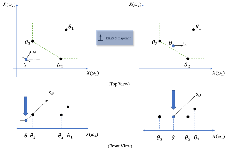
Figure 1: Suppose there are two scenarios ($T=2$) and one attribute ($N=1$), and $\mathcal{D}_{3}=\{\theta_{1},\theta_{2},\theta_{3}\}$. We illustrate the two cases corresponding to $\mathscr{P}_{D}(\theta;\,\mathcal{D}_{3})$, with both top view (upper) and front view (lower). In both cases, suppose $v^{*}_{\theta_{1}}>v^{*}_{\theta_{2}}=v^{*}_{\theta_{3}}$. The upper subgradient must satisfy $s_{\theta}\geq 0$ so it is restricted to lie between the grey dashed lines. When $\theta$ is located on the left hand side of the green dashed line, $\left\langle s_{\theta},\theta^{\prime}-\theta\right\rangle>0$ holds for all $\theta^{\prime}\in\mathcal{D}_{3}$ so that we can push $v_{\theta}$ value strictly lower than $v^{*}_{\theta_{3}}$ as long as the constraint $v_{\theta}+\left\langle s_{\theta},\theta^{\prime}-\theta\right\rangle\geq v^{*}_{\theta^{\prime}},\,\forall\theta^{\prime}\in\mathcal{D}_{3}$ holds. Hence we have $\textsf{val}(\mathscr{P}_{LP}(\theta;\,\mathcal{D}_{3}))=\textsf{val}(\mathscr{P}_{D}(\theta;\,\mathcal{D}_{3}))<v^{*}_{\theta_{3}}$ (left). When $\theta$ is located on the right hand side of the green dashed line, $\left\langle s_{\theta},\theta^{\prime}-\theta\right\rangle>0$ does not hold for all $\theta^{\prime}\in\mathcal{D}_{3}$ and we have $\textsf{val}(\mathscr{P}_{D}(\theta;\,\mathcal{D}_{3}))=v^{*}_{\theta_{3}}$ (right).

Initialization: ${\Theta}$, $j=1$, and $\mathcal{D}_{j}=\{\theta_{1},0\}$;

while $j<J$ do

        Choose $\theta_{j+1}\in\arg\max_{\theta\in{\cal D}\backslash\mathcal{D}_{j}}\pi(\theta;\,\mathcal{D}_{j})$, and set $v_{\theta_{j+1}}:=\pi(\theta_{j+1};\,\mathcal{D}_{j})$;

       

       Update $\mathcal{D}_{j+1}:=\{\mathcal{D}_{j},(\theta_{j+1},v_{\theta_{j+1}})\}$, and set $j:=j+1$;

       

end while

return $\mathcal{D}:=\mathcal{D}_{J}$.

Algorithm 1 Sorting algorithm for decomposition of ${\cal D}$.

The details of our sorting procedure are summarized in Algorithm 1. For fixed $j\in[J]$, we see that Algorithm 1 solves at most $|{\cal D}\backslash{\cal D}_{j}|$ instances of Problem (9). In Case 1, $\theta_{j+1}$ is added to ${\cal D}_{j}$ with RCF value $v^{*}_{\theta_{j+1}}<v^{*}_{\theta_{j}}$. In Case 2, $\theta_{j+1}$ is added to ${\cal D}_{j}$ with RCF value $v^{*}_{\theta_{j+1}}=v^{*}_{\theta_{j}}$. Note that if we encounter $\theta^{\prime}\in{\cal D}\backslash{\cal D}_{j}$ which falls into Case 2, then the RCF at $\theta^{\prime}$ achieves $v^{*}_{\theta_{j}}$. This $\theta^{\prime}$ is then chosen as $\theta_{j+1}$, and there is no need to solve Problem (9) for other $\theta$ in ${\cal D}\backslash{\cal D}_{j}$.

Next we demonstrate Algorithm 1 on Example 3.1, where only LPs are solved.

Example 3.2.

Consider iteration $j=3$ of Algorithm 1 on the setting of Example 3.1. Since $v^{*}_{\theta_{4}}<v^{*}_{\theta_{5}}=v^{*}_{\theta_{6}}$ by assumption, we have

$$v^{*}_{\theta_{4}}=\textsf{val}(\mathscr{P}_{LP}(\theta_{4};\,\mathcal{D}_{3}))=\textsf{val}(\mathscr{P}_{D}(\theta_{4};\,\mathcal{D}_{3}))=\pi(\theta_{4};\,\mathcal{D}_{3})<v^{*}_{\theta_{3}}.$$

In the case where $\textsf{val}(\mathscr{P}_{LP}(\theta_{5};\,\mathcal{D}_{3}))<\textsf{val}(\mathscr{P}_{LP}(\theta_{6};\,\mathcal{D}_{3}))$ holds (i.e., $\pi(\theta_{5};\,\mathcal{D}_{3})\leq\pi(\theta_{6};\,\mathcal{D}_{3})$), we have

$$v^{*}_{\theta_{6}}=\pi(\theta_{6};\,\mathcal{D}_{3})=\textsf{val}(\mathscr{P}_{D}(\theta_{6};\,\mathcal{D}_{3}))\quad\text{and}\quad v^{*}_{\theta_{5}}\geq\pi(\theta_{5};\,\mathcal{D}_{3})=\textsf{val}(\mathscr{P}_{D}(\theta_{5};\,\mathcal{D}_{3})),$$

and consequently $\theta_{6}$ is picked to give ${\cal D}_{4}=\{(\theta_{1},v^{*}_{\theta_{1}}),(\theta_{2},v^{*}_{\theta_{2}}),(\theta_{3},v^{*}_{\theta_{3}}),(\theta_{6},v^{*}_{\theta_{6}})\}$. Alternatively, if $\textsf{val}(\mathscr{P}_{LP}(\theta_{5};\,\mathcal{D}_{3}))\geq\textsf{val}(\mathscr{P}_{LP}(\theta_{6};\,\mathcal{D}_{3}))$ holds (i.e., $\pi(\theta_{5};\,\mathcal{D}_{3})\geq\pi(\theta_{6};\,\mathcal{D}_{3})$), then we have

$$v^{*}_{\theta_{5}}=\pi(\theta_{5};\,\mathcal{D}_{3})=\textsf{val}(\mathscr{P}_{D}(\theta_{5};\,\mathcal{D}_{3}))\quad\text{and}\quad v^{*}_{\theta_{6}}\geq\pi(\theta_{6};\,\mathcal{D}_{3})=\textsf{val}(\mathscr{P}_{D}(\theta_{6};\,\mathcal{D}_{3})),$$

and so $\theta_{5}$ is picked to give ${\cal D}_{4}=\{(\theta_{1},v^{*}_{\theta_{1}}),(\theta_{2},v^{*}_{\theta_{2}}),(\theta_{3},v^{*}_{\theta_{3}}),(\theta_{5},v^{*}_{\theta_{5}})\}$. $\Box$

Theorem 3.4.

We can compute the optimal solution $v^{\ast}=(v_{\theta}^{\ast})_{\theta\in\Theta}$ of $\mathscr{P}$ after solving at most $O(J^{2})$ instances of Problem (9).

In our experiments, we will see that, in line with Theorem 3.4, the computational complexity of our sorting algorithm grows much more slowly in the size of the ECDS $\mathcal{E}$ compared to the convex hull reformulation of $\mathscr{P}$ (see Table 1 and Table 2). The complexity of our model mostly depends on $J$ (which determines the number of LPs we need to solve). It is relatively less sensitive to the number of attributes $N$ and scenarios $T$, because they only affect the size of the LP in each instance and LPs can be solved very efficiently.

3.4 Solving the interpolation problem

After obtaining the optimal solution $v^{*}$ of $\mathscr{P}$, we can evaluate the RCF for any prospect $\vec{X}$ by solving $\mathscr{P}(\vec{X};v^{*})$. Following similar arguments to those in Subsection 3.3, solving $\mathscr{P}(\vec{X};v^{*})$ is equivalent to calculating $\pi(\vec{X};\,\mathcal{D}_{j})$ for the index $j$ which satisfies:

$$v^{*}_{\theta_{j+1}}<\psi_{\mathscr{R}(\mathcal{E})}(\vec{X})\leq v^{*}_{\theta_{j}}.$$ (11)

In order for Eq. (11) to have a solution for all values of $\psi_{\mathscr{R}(\mathcal{E})}(\vec{X})$, we artificially define $\theta_{J+1}:=-\infty$ to be a constant prospect with value $v^{*}_{\theta_{J+1}}:=-\infty$, and we set $\mathcal{D}_{J+1}:=\{\mathcal{D}_{J},(\theta_{J+1},-\infty)\}$. We will identify the correct index $j$ by solving a sequence of instances of $\mathscr{P}_{LP}(\vec{X};\,\mathcal{D}_{j})$, based on the relationships in the next proposition.

Proposition 3.5.

Suppose Eq. (11) holds for $j$.

(i) $\pi(\vec{X};\,\mathcal{D}_{j})=\min\{v^{*}_{\theta_{j}},\textsf{val}(\mathscr{P}_{LP}(\vec{X};\,\mathcal{D}_{j}))\}=\psi_{\mathscr{R}(\mathcal{E})}(\vec{X})$. Moreover, $\textsf{val}(\mathscr{P}_{LP}(\vec{X};\,\mathcal{D}_{j^{\prime}}))\geq\psi_{\mathscr{R}(\mathcal{E})}(\vec{X})$ for all $j^{\prime}\geq j$, and $\textsf{val}(\mathscr{P}_{LP}(\vec{X};\,\mathcal{D}_{j^{\prime}}))\leq\psi_{\mathscr{R}(\mathcal{E})}(\vec{X})$ for all $j^{\prime}<j$.

(ii) $\textsf{val}(\mathscr{P}_{LP}(\vec{X};\,\mathcal{D}_{j^{\prime}}))>v^{*}_{\theta_{j^{\prime}+1}}$ for all $j^{\prime}\geq j$, and $\textsf{val}(\mathscr{P}_{LP}(\vec{X};\,\mathcal{D}_{j^{\prime}}))\leq v^{*}_{\theta_{j^{\prime}+1}}$ for all $j^{\prime}<j$.

Proposition 3.5(i) is a direct consequence of Eq. (10) and the fact that $\mathscr{P}_{LP}(\vec{X};\,\mathcal{D}_{j^{\prime}})$ has the same objective but more constraints than $\mathscr{P}_{LP}(\vec{X};\,\mathcal{D}_{j})$ for $j^{\prime}>j$. To establish Proposition 3.5(ii), notice that for $j^{\prime}\geq j$ we have $v^{*}_{\theta_{j^{\prime}+1}}\leq v^{*}_{\theta_{j+1}}$, and

$$\textsf{val}(\mathscr{P}_{LP}(\vec{X};\,\mathcal{D}_{j^{\prime}}))\geq\psi_{\mathscr{R}(\mathcal{E})}(\vec{X})>v^{*}_{\theta_{j+1}}\geq v^{*}_{\theta_{j^{\prime}+1}}.$$

Meanwhile if $j^{\prime}<j$ then $j^{\prime}+1\leq j$ and $v^{*}_{\theta_{j^{\prime}+1}}\geq v^{*}_{\theta_{j}}$. Hence

$$\textsf{val}(\mathscr{P}_{LP}(\vec{X};\,\mathcal{D}_{j^{\prime}}))\leq\psi_{\mathscr{R}(\mathcal{E})}(\vec{X})\leq v^{*}_{\theta_{j}}\leq v^{*}_{\theta_{j^{\prime}+1}}.$$

We can identify the correct $j$ in Eq. (11) by choosing the least element $j^{*}$ of the set $\{j^{\prime}:\textsf{val}(\mathscr{P}_{LP}(\vec{X};\,\mathcal{D}_{j^{\prime}}))>v^{*}_{\theta_{j^{\prime}+1}}\}$, so that $\psi_{\mathscr{R}(\mathcal{E})}(\vec{X})=\pi(\vec{X};\,\mathcal{D}_{j^{*}})$ by Proposition 3.5(i). This procedure is summarized in the following level search algorithm (we call it level search because we are trying to identify an appropriate level for $\textsf{val}(\mathscr{P}_{LP}(\vec{X};\,\mathcal{D}_{j^{\prime}}))$ such that the strict inequality holds).

Input: $\vec{X}\in\mathbb{R}^{TN}$;

Initialization: $h=1$;

while $\textsf{val}(\mathscr{P}_{LP}(\vec{X};\,\mathcal{D}_{h}))\leq v^{*}_{\theta_{h+1}}$ do

        Set $h=h+1$;

       

end while

return $\psi_{\mathscr{R}\left(\mathcal{E}\right)}(\vec{X})=\pi(\vec{X};\,\mathcal{D}_{h})$.

Algorithm 2 Level search for interpolation problem

Level search essentially enumerates the levels and finds $h=j$ after solving at most $O(J)$ instances of $\mathscr{P}_{LP}(\vec{X};\,\mathcal{D}_{j})$. One can further reduce the complexity of solving the interpolation problem to $O(\log J)$ with binary search (see Algorithm 5 in Appendix B).

Theorem 3.6.

Given $\vec{X}\in\mathbb{R}^{TN}$, the value $\psi_{\mathscr{R}(\mathcal{E})}(\vec{X})$ can be computed after solving at most $O(\log J)$ instances of $\mathscr{P}_{LP}(\vec{X};\,\mathcal{D}_{j})$.

4 Law invariant case

In the previous section, we assume that the DM has an unknown choice function $\phi\in\mathfrak{R}$ and may evaluate prospects differently even when they have the same law (i.e., the same outcome distribution on $\mathbb{R}^{N}$). That is, the choice function may not be law invariant. Law invariance is a fundamental property of the preferences when the DMs only care about the outcome distribution. In this section, we incorporate [Law] into our RCF.

To begin, we introduce a reference probability measure $\mathbb{P}$ on $\Omega$ to assign distributions to prospects in $\mathcal{L}^{N}$ (formally, the distribution $\mathbb{P}\circ X^{-1}$ on $\mathbb{R}^{N}$ for any $X\in\mathcal{L}^{N}$).

Assumption 4.1.

The probability measure $\mathbb{P}$ satisfies $\mathbb{P}(\omega_{t})=1/T$ for all $t\in[T]$.

This assumption is without loss of generality if $\mathbb{P}$ takes rational values on $\Omega$. When $\mathbb{P}$ has rational values we can just take the underlying sample space to be sufficiently large and give $\mathbb{P}$ equal weight to recover any desired rational probability (see Delage and Li (2017)). The empirical probability measure in sample average approximation automatically satisfies this assumption.

Let $\Sigma$ denote the set of all permutations on $\Omega$. Under Assumption 4.1, we can encode [Law] in terms of $\Sigma$. For a permutation $\sigma\in\Sigma$, we permute the sample space $\Omega$ as $\sigma(\Omega)=\{\omega_{\sigma(1)},\omega_{\sigma(2)},\ldots,\omega_{\sigma(T)}\}$. Similarly, we permute $\vec{X}=(X(\omega_{t}))_{t=1}^{T}$ as $\sigma(\vec{X})=(X(\omega_{\sigma(t)}))_{t=1}^{T}$. A law invariant choice function $\phi\in\mathfrak{R}$ must satisfy $\phi(\vec{X})=\phi(\sigma(\vec{X}))$ for all $\vec{X}\in\mathbb{R}^{TN}$ and $\sigma\in\Sigma$, since $\vec{X}$ and $\sigma(\vec{X})$ have the same distribution on $\mathbb{R}^{N}$.

Let $F_{X}$ denote the distribution of $X\in\mathcal{L}^{N}$. Then, under [Law] and Assumption 4.1, we can characterize the DM’s preferences in terms of outcome distributions. In particular, the relation $F_{W}\succeq F_{Y}$ is equivalent to $\phi(\sigma(W))\geq\phi(\sigma^{\prime}(Y))$ for all $\sigma,\,\sigma^{\prime}\in\Sigma$. The ECDS can then be expressed equivalently in terms of distributions as $\mathcal{E}=\{(F_{W_{k}},\,F_{Y_{k}})\}_{k\in[K]}$, where the DM weakly prefers $F_{W_{k}}$ to $F_{Y_{k}}$ for all $k\in[K]$.

Similar to Section 2, we make the following assumption on the DM’s preferences so that our law invariant RCF is well-defined.

Assumption 4.2.

The DM’s preferences can be described by a choice function in $\mathfrak{R}\cap\mathscr{R}_{\text{Law}}\cap\mathscr{R}_{\text{Eli}}(\mathcal{E})$.

Recall $\mathscr{R}_{L}\left(\mathcal{E}\right)$ is the ambiguity set for law-invariant choice functions. We give an optimization formulation for $\psi_{\mathscr{R}_{L}\left(\mathcal{E}\right)}(\vec{X})$. Recall $\Theta=\{\vec{W}_{0},\vec{W}_{1},\,\vec{Y}_{1},\ldots,\vec{W}_{K},\vec{Y}_{K}\}$ is the set of prospects used in the construction of the RCF. We define the augmented support set

$$\Theta_{L}:=\cup_{\sigma\in\Sigma}\left\{\sigma(\theta)\mid\theta\in\Theta\right\}$$

with cardinality $J_{L}:=(2K+1)|\Sigma|$. Then, we define

$$\widehat{\Theta}_{L}:=\left\{\left(\theta,\,\theta^{\prime}\right)\in\Theta_{L}\times\Theta_{L}\text{ : }\theta\neq\theta^{\prime}\right\}$$

to be the set of all edges in $\Theta_{L}$. Finally, we define the augmented ECDS

$$\mathcal{E}_{L}:=\left\{\left(\sigma(\theta),\,\sigma^{\prime}(\theta^{\prime})\right)\text{ : }(\theta,\theta^{\prime})\in\mathcal{E},\,\sigma,\,\sigma^{\prime}\in\Sigma\right\}$$

to be the set of all permutations of pairs in $\mathcal{E}$. We obtain the following formulation for $\psi_{\mathscr{R}_{L}\left(\mathcal{E}\right)}(\vec{X})$, the proof is similar to Theorem 3.1.

Theorem 4.3.

For any $\vec{X}\in\mathbb{R}^{TN}$, $\psi_{\mathscr{R}_{L}\left(\mathcal{E}\right)}(\vec{X})$ is equal to the optimal value of:

$$\min_{v_{L},\,s_{L},\,v_{X},\,s_{X}}\, v_{X}$$ (12a)

s.t. $$v_{\theta}+\max\left\{\langle s_{\theta},\,\theta^{\prime}-\theta\rangle,\,0\right\}\geq v_{\theta^{\prime}},\quad\forall\left(\theta,\,\theta^{\prime}\right)\in\widehat{\Theta}_{L},$$ (12g)

$$s_{\theta}\geq 0,\,\|s_{\theta}\|_{1}\leq C,\quad\forall\theta\in\Theta_{L},$$

$$v_{\theta}\geq v_{\theta^{\prime}},\quad\forall\left(\theta,\,\theta^{\prime}\right)\in\mathcal{E}_{L},$$

$$v_{\sigma(W_{0})}=0,\,\forall\sigma\in\Sigma,$$

$$v_{X}+\max\{\langle s_{X},\,\theta-\vec{X}\rangle,\,0\}\geq v_{\theta},\quad\forall\theta\in\Theta_{L},$$

$$s_{X}\geq 0,\,\|s_{X}\|_{1}\leq C,$$

where $v_{L}=(v_{\theta})_{\theta\in\Theta_{L}}\in\mathbb{R}^{|\Theta_{L}|}$ and $v_{X}$ correspond to the values of the kinked majorants, and $s_{L}=(s_{\theta})_{\theta\in\Theta_{L}}\in\mathbb{R}^{|\Theta_{L}|TN}$ and $s_{X}$ corresponds to the upper subgradients.

Law invariance adds a computational cost to Problem (12) over the base case since there is now an exponential number of constraints due to the indexing by permutations.

We will develop a two-stage decomposition scheme for evaluation of $\psi_{\mathscr{R}_{L}\left(\mathcal{E}\right)}$ by leveraging our results for the base case. The law invariant value problem is:

$$(\mathscr{P}_{L})\qquad\min_{v_{L},\,s_{L}}\, \sum_{\theta\in\Theta_{L}}v_{\theta}$$ (13a)

s.t. $$v_{\theta}+\max\left\{\langle s_{\theta},\,\theta^{\prime}-\theta\rangle,\,0\right\}\geq v_{\theta^{\prime}},\quad\forall\left(\theta,\,\theta^{\prime}\right)\in\widehat{\Theta}_{L},$$ (13e)

$$s_{\theta}\geq 0,\,\|s_{\theta}\|_{1}\leq C,\quad\forall\theta\in\Theta_{L},$$

$$v_{\theta}\geq v_{\theta^{\prime}},\quad\forall\left(\theta,\,\theta^{\prime}\right)\in\mathcal{E}_{L},$$

$$v_{\sigma(W_{0})}=0,\quad\forall\sigma\in\Sigma.$$

Problem $\mathscr{P}_{L}$ is similar to $\mathscr{P}$, except that it has an exponential number of variables in $(v_{L},s_{L})$, and an exponential number of constraints in Eqs. (13e) - (13e). For values $v_{L}=(v_{\theta})_{\theta\in\Theta_{L}}$, the law invariant interpolation problem is:

$$(\mathscr{P}_{L}(\vec{X};\,v_{L}))\qquad\min_{v_{X},\,s_{X}}\, v_{X}$$ (14a)

s.t. $$v_{X}+\max\{\langle s_{X},\,\theta-\vec{X}\rangle,\,0\}\geq v_{\theta},\quad\forall\theta\in\Theta_{L},$$ (14c)

$$s_{X}\geq 0,\,\|s_{X}\|_{1}\leq C.$$

Problem $\mathscr{P}_{L}(\vec{X};\,v_{L})$ is similar to $\mathscr{P}(\vec{X};\,v)$ except that it has an exponential number of majorization constraints (but it does have the same variables which determine a single kinked majorant at $\vec{X}$).

In the next proposition we confirm that an optimal solution of $\mathscr{P}_{L}$ exists and is unique. Furthermore, we show that the values $v_{\sigma(\theta)}^{\ast}$ at the optimal solution are invariant under permutation.

Proposition 4.4.

Problem $\mathscr{P}_{L}$ has a unique optimal solution $v^{*}_{L}=(v_{\theta}^{*})_{\theta\in\Theta_{L}}$. Furthermore, $v^{*}_{\sigma(\theta)}=v^{*}_{\sigma^{\prime}(\theta)}$ for all $\theta\in\Theta$ and $\sigma,\sigma^{\prime}\in\Sigma$.

It follows that we only need to compute $v^{*}_{\theta}$ for each $\theta\in\Theta$, and then we can assign this same value to all permutations of $\theta$. We may then characterize the optimal solution of $\mathscr{P}_{L}$ with $v^{*}=(v_{\theta}^{*})_{\theta\in\Theta}\in\mathbb{R}^{|\Theta|}$ instead of $v_{L}^{*}=(v_{\theta}^{*})_{\theta\in\Theta_{L}}\in\mathbb{R}^{|\Theta_{L}|}$. Subsequently, $\mathscr{P}_{L}(\vec{X};\,v_{L}^{*})$ reduces to:

$$(\mathscr{P}_{L}(\vec{X};\,v^{*}))\qquad\min_{v_{X},\,s_{X}}\, v_{X}$$ (15a)

s.t. $$v_{X}+\max\{\langle s_{X},\,\sigma(\theta)-\vec{X}\rangle,\,0\}\geq v_{\theta},\quad\forall\theta\in\Theta,\,\sigma\in\Sigma,$$ (15c)

$$s_{X}\geq 0,\,\|s_{X}\|_{1}\leq C.$$

We emphasize that this reduction is specific to the optimal solution $v_{L}^{*}$ of $\mathscr{P}_{L}$, and does not necessarily hold for arbitrary $v_{L}\in\mathbb{R}^{|\Theta_{L}|}$.

We now have the following two-stage decomposition result which connects the law invariant value and interpolation problems.

Theorem 4.5.

Let $v^{*}$ be the optimal solution of $\mathscr{P}_{L}$. Then, $v_{\theta}^{*}=\psi_{\mathscr{R}_{L}\left(\mathcal{E}\right)}\left(\theta\right)$ for all $\theta\in\Theta$. Furthermore, $\psi_{\mathscr{R}_{L}\left(\mathcal{E}\right)}(\vec{X})=\textsf{val}(\mathscr{P}_{L}(\vec{X};\,v^{\ast}))$ for all $\vec{X}\in\mathbb{R}^{TN}$.

Since we only have to determine the values of the law-invariant RCF on $\Theta$, we can solve $\mathscr{P}_{L}$ with a decomposition of $\Theta$ (instead of the much larger set $\Theta_{L}$). We denote this decomposition as $\{\mathcal{D}_{L,j}\}_{j\in[J]}$ and $\mathcal{D}_{L}=\mathcal{D}_{L,j}$ to distinguish the law invariant case. Given $\mathcal{D}_{L,j}:=\{(\theta_{1},v_{\theta_{1}}^{*}),\ldots,(\theta_{j},v_{\theta_{j}}^{*})\}$ for $j\in[J]$, we define $\Sigma(\mathcal{D}_{L,j}):=\{(\sigma(\theta),v_{\sigma(\theta)}^{\ast})_{\sigma\in\Sigma}\}_{\theta\in\mathcal{D}_{L,j}}$ to be the ordered list containing all permutations of prospects in $\mathcal{D}_{L,j}$. We know $v^{*}_{\sigma(\theta)}=v^{*}_{\theta}$ for all $\theta\in\Theta$ and $\sigma\in\Sigma$, we can seat all permutations of the same $\theta$ next to each other in $\Sigma(\mathcal{D}_{L,j})$ since they are sorted by value.

For $\theta\in\Theta$ and $\Sigma(\mathcal{D}_{L,j})$, we define the following LP:

$$(\mathscr{P}_{LP}(\theta;\,\Sigma(\mathcal{D}_{L,j})))\qquad\min_{v_{\theta},s_{\theta}}\quad v_{\theta}$$ (16a)

s.t. $$v_{\theta}+\left\langle s_{\theta},\sigma(\theta^{\prime})-\theta\right\rangle\geq v^{*}_{\theta^{\prime}},\,\forall\theta^{\prime}\in\mathcal{D}_{L,j},\,\sigma\in\Sigma,$$ (16b)

$$s_{\theta}\geq 0,\left\|s_{\theta}\right\|_{1}\leq C,$$ (16c)

$$v_{\theta}\geq v^{*}_{\theta^{\prime}},\quad\forall(\theta,\theta^{\prime})\in{\mathcal{E}},\theta^{\prime}\in\mathcal{D}_{L,j}.$$ (16d)

Problem $\mathscr{P}_{LP}(\theta;\,\Sigma(\mathcal{D}_{L,j}))$ has an exponential number of constraints, but we can reduce it to a more tractable problem with a polynomial number of constraints (see Delage and Li (2017) where this idea is used for PRO with convex monetary risk measures). This reduction is based on strong duality results for the binary assignment problem.

Let $\theta_{n}:=(\theta_{n}(\omega_{t}))_{t\in[T]}$ be the vector of realizations corresponding to attribute $n\in[N]$ of $\theta$. For an upper subgradient $s=(s_{t,n})_{t\in[T],\,n\in[N]}\in\mathbb{R}^{TN}$ corresponding to a kinked majorant, let $s_{n}=(s_{t,n})_{t\in[T]}\in\mathbb{R}^{T}$ be the vector of realizations of $s$ corresponding to attribute $n$. We also let $\mathbf{1}_{T}$ denote the unit vector in $\mathbb{R}^{T}$, and $\top$ denote the transpose operation. For $j\in[J]$, the reduced LP is:

$$\mathscr{P}_{L,LP}(\theta;\,\mathcal{D}_{L,j}):=\min_{s,v_{\theta},\{y_{\theta^{\prime}},w_{\theta^{\prime}}\}_{\theta^{\prime}\in\mathcal{D}_{L,j}}} \quad v_{\theta}$$ (17a)

s.t. $$\mathbf{1}_{T}^{\top}y_{\theta^{\prime}}+\mathbf{1}_{T}^{\top}w_{\theta^{\prime}}-\langle s,\theta\rangle+v_{\theta}-v^{*}_{\theta^{\prime}}\geq 0,\quad\forall\theta^{\prime}\in\mathcal{D}_{L,j},$$ (17b)

$$\sum^{N}_{n=1}\theta^{\prime}_{n}s_{n}^{\top}-y_{\theta^{\prime}}\mathbf{1}_{T}^{\top}-\mathbf{1}_{T}w_{\theta^{\prime}}^{\top}\geq 0,\quad\forall\theta^{\prime}\in\mathcal{D}_{L,j},$$ (17c)

$$s\geq 0,\left\|s\right\|_{1}\leq C,$$ (17d)

$$v_{\theta}=v^{*}_{\theta^{\prime}},\quad\forall(\theta,\theta^{\prime})\in\mathcal{E},\theta^{\prime}\in\mathcal{D}_{L,j},$$ (17e)

$$y_{\theta^{\prime}},w_{\theta^{\prime}}\in\mathbb{R}^{T},\,\forall\theta^{\prime}\in\mathcal{D}_{L,j},$$ (17f)

$$s\in\mathbb{R}^{TN},v_{\theta}\in\mathbb{R}.$$ (17g)

Note the LHS of Constraint (17c) is a $T\times T$ matrix, so this inequality is understood to hold component-wise. In particular, note that $\mathscr{P}_{L,LP}(\theta;\,\mathcal{D}_{L,j})$ has a polynomial number of constraints. We justify the reduction from $\mathscr{P}_{L}(\theta;\,\mathcal{D}_{L,j})$ to $\mathscr{P}_{L,LP}(\theta;\,\Sigma(\mathcal{D}_{L,j}))$ in the following proposition.

Proposition 4.6.

For all $j\in[J]$ and $\theta\in\Theta$, $\textsf{val}(\mathscr{P}_{L,LP}(\theta;\,\mathcal{D}_{L,j}))=\textsf{val}(\mathscr{P}_{LP}(\theta;\,\Sigma(\mathcal{D}_{L,j})))$.

The law invariant sorting algorithm for $\mathscr{P}_{L}$ is as follows (see Algorithm 6 in Appendix C for the detailed steps). Given $\mathcal{D}_{L,j}$, we compute the law invariant predictor

$$\pi_{L}(\theta;\,\mathcal{D}_{L,j}):=\min\{v^{*}_{\theta_{j}},\textsf{val}(\mathscr{P}_{L,LP}(\theta;\,\mathcal{D}_{L,j}))\},\,\forall\theta\notin\mathcal{D}_{L,j}.$$

Then, one of the prospects $\theta\notin\mathcal{D}_{L,j}$ that maximizes $\pi_{L}(\theta;\,\mathcal{D}_{L,j})$, as well as its predicted value, is chosen to append to $\mathcal{D}_{L,j}$, and we proceed to the next iteration. The algorithm terminates with a decomposition $\mathcal{D}_{L}=\mathcal{D}_{L,J}$. The next theorem gives the computational complexity for solving $\mathscr{P}_{L}$ using this method.

Theorem 4.7.

We compute the optimal solution $v^{\ast}=(v_{\theta}^{\ast})_{\theta\in\Theta}$ of $\mathscr{P}_{L}$ after solving at most $O(J^{2})$ instances of Problem (17).

We note the same order of complexity for the law invariant sorting algorithm compared to the base sorting algorithm (i.e., it is $J$ rather than $J_{L}$). We may also use binary search to solve the law invariant interpolation problem (see Algorithm 8), with the same logarithmic complexity as the base case.

Theorem 4.8.

Given $\vec{X}\in\mathbb{R}^{TN}$, the value $\psi_{\mathscr{R}_{L}(\mathcal{E})}(\vec{X})$ can be computed after solving at most $O(\log J)$ instances of Problem (17).

In particular, the complexity of law invariant binary search for the interpolation problem depends on $J$ rather than $J_{L}$.

5 Acceptance set representation

In this section we construct the acceptance sets of the RCF. This construction gives another representation of the RCF in terms of the epigraph formulation. Furthermore, this construction leads to our method for doing PRO efficiently.

The acceptance set at level $v\in\mathbb{R}$ induced by the RCF is

$$\mathcal{A}_{v}:=\{\vec{X}\in\mathbb{R}^{TN}:\psi_{\mathscr{R}\left(\mathcal{E}\right)}(\vec{X})\geq v\},\,\forall v\in\mathbb{R}.$$

The epigraphical representation of the RCF in terms of its acceptance sets is:

$$\psi_{\mathscr{R}\left(\mathcal{E}\right)}(\vec{X})=\sup_{v\in\mathbb{R}}\{v:\vec{X}\in\mathcal{A}_{v}\},\,\forall\vec{X}\in\mathbb{R}^{TN}.$$ (18)

Eq. (18) will be useful for optimization of the RCF in the next section, after we identify the explicit form of the acceptance sets.

We construct $\{\mathcal{A}_{v}\}_{v\leq 0}$ based on the optimal solution of $\mathscr{P}$ (the normalizing prospect is canonically the most preferred so all prospects considered will have non-positive RCF values). This construction is based on a level selection rule which maps a level $v$ to a subset of prospects in $\Theta$, which is then used to construct the corresponding $\mathcal{A}_{v}$. Recall that $\theta_{J+1}=-\infty$ has value $v^{*}_{\theta_{J+1}}=-\infty$, and $\mathcal{D}_{J+1}=\{\mathcal{D}_{J},(\theta_{J+1},-\infty)\}$.

Definition 5.1 (Level selection).

Given $v\leq 0$, $\kappa(v):=\{j\in[J+1]\mid v^{*}_{\theta_{j+1}}<v\leq v^{*}_{\theta_{j}}\}$.

For $v$ and $j=\kappa(v)$, we use the prospects in $\mathcal{D}_{j}$ to construct $\mathcal{A}_{v}$. The level selection rule enforces the condition $v^{*}_{\theta_{j+1}}<v\leq v^{*}_{\theta_{j}}$ corresponding to Eq. (11). The selection $j=\kappa(v)$ is unique under this convention since we must always choose $j$ with $v^{*}_{\theta_{j+1}}<v^{*}_{\theta_{j}}$. There may be $j$ with $v^{*}_{\theta_{j+1}}=v^{*}_{\theta_{j}}$ (i.e., repeated values), but such $j$ are never selected. If there are multiple indices which give the same value $v^{\ast}_{\theta_{j}}$, then $\kappa(\cdot)$ will return the largest such index.

The next proposition shows that we can check if $\vec{X}\in\mathcal{A}_{v}$ by solving $\mathscr{P}_{LP}(\vec{X};\,\mathcal{D}_{j})$ for $j=\kappa(v)$. It is based on the dependence of $\mathcal{A}_{v}$ on $\mathcal{D}_{j}$ for $j=\kappa(v)$.

Proposition 5.1.

For $v\leq 0$ and $j=\kappa(v)$, $\psi_{\mathscr{R}\left(\mathcal{E}\right)}(\vec{X})\geq v$ if and only if $\textsf{val}(\mathscr{P}_{LP}(\vec{X};\,\mathcal{D}_{j}))\geq v$.

The previous proposition leads to the characterization of $A_{v}$ by linear programming duality.

We denote the LP dual of $\mathscr{P}_{LP}(\vec{X};\,\mathcal{D}_{j})$ by $\mathscr{D}_{LP}(\vec{X};\,\mathcal{D}_{j})$ (see the explicit formulation in Eqs. (47a)-(47c)). By strong duality, we have $\textsf{val}(\mathscr{P}_{LP}(\vec{X};\,\mathcal{D}_{j}))=\textsf{val}(\mathscr{D}_{LP}(\vec{X};\,\mathcal{D}_{j}))$ and so the inequality $\textsf{val}(\mathscr{P}_{LP}(\vec{X};\,\mathcal{D}_{j}))\geq v$ is equivalent to $\textsf{val}(\mathscr{D}_{LP}(\vec{X};\,\mathcal{D}_{j}))\geq v$. Since $\mathscr{D}_{LP}(\vec{X};\,\mathcal{D}_{j})$ is a maximization problem, $\textsf{val}(\mathscr{D}_{LP}(\vec{X};\,\mathcal{D}_{j}))\geq v$ is just a feasibility problem, and its constraints lead to the explicit acceptance set representation in the following theorem. Let $\mathbf{1}_{TN}\in\mathbb{R}^{TN}$ be the vector with all components equal to one. We define translations of the prospects in $\Theta$ by $\tilde{\theta}:=\theta-(v^{*}_{\theta}/C)\mathbf{1}_{TN}$ (where we subtract $v^{*}_{\theta}/C$ from every component of $\theta$).

Theorem 5.2.

For $v\leq 0$,

$$\mathcal{A}_{v}=\left\{\vec{X}\in\mathbb{R}^{TN}\mid\vec{X}\geq\sum_{\theta\in\mathcal{D}_{\kappa(v)}}\tilde{\theta}\cdot p_{\theta}+(v/C)\mathbf{1}_{TN},\,\sum_{\theta\in\mathcal{D}_{\kappa(v)}}p_{\theta}=1,\,p\in\mathbb{R}^{\kappa(v)}_{\geq 0}\right\}.$$

Theorem 5.2 shows that the acceptance sets have a piecewise linear structure, and that checking $\vec{X}\in\mathcal{A}_{v}$ can be done by solving a linear feasibility problem. In view of $\tilde{\theta}$ as a translation of $\theta$, we can interpret $\mathcal{A}_{v}$ as the smallest monotone polyhedron that contains the convex hull of all translations $\tilde{\theta}$ of prospects $\theta$ for which $v^{*}_{\theta}\geq v$.

The law invariant case follows the same idea. The acceptance sets of $\psi_{\mathscr{R}_{L}(\mathcal{E})}$ are:

$$\mathcal{A}_{L,v}:=\{\vec{X}\in\mathbb{R}^{TN}:\psi_{\mathscr{R}_{L}\left(\mathcal{E}\right)}(\vec{X})\geq v\},\,\forall v\in\mathbb{R},$$

and the epigraphical representation is:

$$\psi_{\mathscr{R}_{L}\left(\mathcal{E}\right)}(\vec{X})=\sup\{v:\vec{X}\in\mathcal{A}_{L,v}\},\,\forall\vec{X}\in\mathbb{R}^{TN}.$$ (19)

By strong linear programming duality (see Eqs. (49) for the dual of $\mathscr{P}_{L,LP}(\vec{X};\,\mathcal{D}_{L,j})$), we arrive at the following characterization of the law invariant acceptance sets.

Theorem 5.3.

For all $v\leq 0$, we have

$$\mathcal{A}_{L,v}=\left\{\begin{array}[]{l|l}\vec{X}\in\mathbb{R}^{TN}&\begin{array}[]{l}\sum_{\theta\in\mathcal{D}_{L,\kappa(v)}}v^{*}_{\theta}\cdot p_{\theta}-C\,q\geq v,\\ \sum_{\theta\in\mathcal{D}_{L,\kappa(v)}}\rho_{\theta}^{\top}\cdot\theta_{n}-\vec{X}_{n}\leq q\cdot\mathbf{1}_{T},\quad\forall n\in[N]\\ \sum_{\theta\in\mathcal{D}_{L,\kappa(v)}}p_{\theta}=1,\,p\in\mathbb{R}^{\kappa(v)}_{\geq 0},\,q\geq 0,\\ \mathbf{1}_{T}^{\top}\rho_{\theta}=p_{\theta}\mathbf{1}_{T}^{\top},\,\rho_{\theta}\mathbf{1}_{T}=p_{\theta}\mathbf{1}_{T}^{\top},\,\rho_{\theta}\in\mathbb{R}_{\geq 0}^{T\times T},\quad\forall\theta\in\mathcal{D}_{L,\kappa(v)}\end{array}\end{array}\right\}.$$

Theorem 5.3 shows that the law invariant acceptance sets also have a piecewise linear structure, and checking $\vec{X}\in\mathcal{A}_{L,v}$ can similarly be done by solving a linear feasibility problem. The representation of $\mathcal{A}_{L,v}$ in Theorem 5.3 is based on the dual of the reduced LP $\mathscr{P}_{L,LP}(\vec{X};\,\mathcal{D}_{L,j})$, rather than $\mathscr{P}_{LP}(\vec{X};\,\Sigma(\mathcal{D}_{L,j}))$, and so it has a polynomial number of variables and constraints.

6 Preference robust optimization

Now suppose the DM wants to optimize over a set of admissible prospects. In the face of ambiguity about the DM’s preferences, we cannot precisely identify a choice function to optimize, so we optimize the RCF. We show that this problem can be solved efficiently based on the acceptance set representation.

The DM’s optimization problem is as follows. Let $\mathcal{Z}\subset\mathbb{R}^{M}$ be a set of feasible decisions for $M\geq 1$. Then, let $G:\mathcal{Z}\to\mathcal{L}^{N}$ be a stochastic reward function where $G(z,\omega):=(G_{n}(z,\omega))_{n\in[N]}\in\mathbb{R}^{N}$ is the vector of rewards/gains on scenario $\omega\in\Omega$. Under Assumption 2.1, the stochastic function $G(z)$ can be expressed in vector form $\vec{G}(z)=(G(z,\omega))_{\omega\in\Omega}\in\mathbb{R}^{TN}$ for any $z\in\mathcal{Z}$. The following assumptions are typical in the stochastic optimization literature (see, e.g., Shapiro et al. (2014)).

Assumption 6.1.

(i) $\mathcal{Z}$ is compact and convex.

(ii) $\vec{G}$ is concave (i.e., $z\to G(z,\omega)$ is concave in the vector-valued sense with respect to $\mathbb{R}_{\geq 0}^{N}$ for all $\omega\in\Omega$).

Given a preference relation $\succeq$ and a corresponding choice function $\phi\in\mathfrak{R}$ representing $\succeq$, we would solve:

$$(\mathscr{P}(\phi))\qquad\max_{z\in\mathcal{Z}}\phi(\vec{G}(z)),$$

to identify an optimal solution $z^{*}$ for the DM. However, $\mathscr{P}(\phi)$ requires complete information about the choice function $\phi$, and the optimal solution of $\mathscr{P}(\phi)$ is highly sensitive to $\phi$.

Faced with this ambiguity, we will optimize the RCF:

$$(\mathscr{P}(\mathscr{R}))\qquad\max_{z\in\mathcal{Z}}\psi_{\mathscr{R}}(\vec{G}(z)),$$

for an ambiguity set $\mathscr{R}\subset\mathfrak{R}$. The objective $z\to\psi_{\mathscr{R}}(\vec{G}(z))$ of $\mathscr{P}(\mathscr{R})$ is quasi-concave under Assumption 6.1 for any $\mathscr{R}\subset\mathfrak{R}$, since the composition of an increasing quasi-concave function with a concave function is quasi-concave. It follows that $\mathscr{P}(\mathscr{R})$ is maximizing a quasi-concave function over a convex set, and so it can be solved via a sequence of convex feasibility problems.

We focus on solving the specific PRO problems $\mathscr{P}(\mathscr{R}(\mathcal{E}))$ and $\mathscr{P}(\mathscr{R}_{L}(\mathcal{E}))$ based on the acceptance sets of the RCF. By the epigraphical representation of the RCF, $\mathscr{P}(\mathscr{R}(\mathcal{E}))$ is equivalent to

$$\max_{z\in\mathcal{Z},\,v\in\mathbb{R}}\{v:\vec{G}(z)\in\mathcal{A}_{v}\}.$$

We can solve the above reformulation of $\mathscr{P}(\mathscr{R}(\mathcal{E}))$ via a sequence of convex feasibility problems of the form:

$$\{z\in\mathcal{Z}:\vec{G}(z)\in\mathcal{A}_{v}\},$$ (20)

where $v\leq 0$ is fixed. Finding the largest $v$ for which Eq. (20) is feasible is equivalent to solving $\mathscr{P}(\mathscr{R}(\mathcal{E}))$. Since we have the explicit form of $\{\mathcal{A}_{v}\}$, we can solve Eq. (20) (or determine it is infeasible) for any $v$.

Conceptually, we can scan over all levels $v\leq 0$ to find the largest $v$ such that Eq. (20) is feasible. However, Theorem 5.2 shows that the acceptance sets have a piecewise linear structure that depends on the level $v$. So, the search over all $v\leq 0$ can be broken up into separate feasibility problems for each $j\in[J+1]$:

$$\{z\in\mathcal{Z},\,v^{*}_{j+1}<v\leq v^{*}_{j}:\vec{G}(z)\in\mathcal{A}_{v}\},$$ (21)

where $v$ is also an optimization variable in Eq. (21).

Based on Theorem 5.2, the feasibility problem corresponding to Eq. (21) is explicitly:

$$(\mathscr{F}(\mathcal{D}_{j}))\qquad\operatorname{Find}\quad z\in\mathcal{Z},\,v^{*}_{j+1}<v\leq v^{*}_{j},\,p\in\mathbb{R}^{j}$$ (22a)

s.t. $$\vec{G}(z)\geq\sum_{\theta\in\mathcal{D}_{j}}\tilde{\theta}\cdot p_{\theta}+(v/C)\mathbf{1}_{TN},$$ (22b)

$$\sum_{\theta\in\mathcal{D}_{j}}p_{\theta}=1,$$ (22c)

$$p\geq 0,$$ (22d)

for each $j\in[J]$. Problem $\mathscr{F}(\mathcal{D}_{j})$ can be interpreted as finding $z\in\mathcal{Z}$ such that the prospect $\vec{G}(z)$ is acceptable at a level $v^{*}_{j+1}<v\leq v^{*}_{j}$.

If $\mathscr{F}(\mathcal{D}_{j})$ is feasible for $j$, then it is feasible for any $j^{\prime}>j$ since $v_{j}^{*}$ are non-increasing in $j$. We want to find the least $j$ such that $\mathscr{F}(\mathcal{D}_{j})$ is feasible. Once we locate such a $j$, we solve the following convex optimization problem:

$$(\mathscr{G}(\mathcal{D}_{j}))\qquad\max_{z\in\mathcal{Z},\,v^{*}_{j+1}<v\leq v^{*}_{j},\,p\in\mathbb{R}^{j}}\quad v$$ (23a)

s.t. $$\vec{G}(z)\geq\sum_{\theta\in\mathcal{D}_{j}}\tilde{\theta}\cdot p_{\theta}+(v/C)\mathbf{1}_{TN},$$ (23b)

$$\sum_{\theta\in\mathcal{D}_{j}}p_{\theta}=1,$$ (23c)

$$p\geq 0,$$ (23d)

which returns the optimal solution and optimal value of $\mathscr{P}(\mathscr{R}(\mathcal{E}))$. We summarize this procedure in the following level search algorithm.

Initialization: $h=1$;

while $\mathscr{F}(\mathcal{D}_{h})$ is infeasible do

        Set $h=h+1$;

       

end while

Compute $v_{h}=\textsf{val}(\mathscr{G}(\mathcal{D}_{h}))$ with optimal solution $z^{*}$;

return $z^{*}$ and $\psi_{\mathscr{R}\left(\mathcal{E}\right)}(G(z^{*}))=v_{h}$.

Algorithm 3 Level search for $\mathscr{P}(\mathscr{R}(\mathcal{E}))$

Algorithm 3 searches over the index set $[J+1]$ and finds the smallest $j$ such that $v_{\theta_{j+1}}^{*}<\psi_{\mathscr{R}\left(\mathcal{E}\right)}(G(z))\leq v_{\theta_{j}}^{*}$ is satisfied for some $z\in\mathcal{Z}$. This search procedure solves $\mathscr{P}(\mathscr{R}(\mathcal{E}))$ after solving at most $O(J)$ instances of $\mathscr{F}(\mathcal{D}_{j})$. We can get better complexity with binary search (see Algorithm 9 in Appendix E).

Theorem 6.2.

Algorithm 9 returns an optimal solution $z^{*}$ of $\mathscr{P}(\mathscr{R}(\mathcal{E}))$, after solving at most $O(\log J)$ instances of Problem (22) and one instance of Problem (23).

The computational complexity $O(\log\,J)$ in Theorem 6.2 follows from the standard complexity of binary search (since we have $J$ alternatives to check). In line with this theorem, our numerical experiments show that the running time of Algorithm 9 is not really sensitive to $J$. It is more sensitive to the problem dimension which is captured by $N$ and $T$ (see Table 4).

The law invariant case is similar, $\mathscr{P}(\mathscr{R}_{L}(\mathcal{E}))$) is equivalent to

$$\max_{z\in\mathcal{Z},\,v\in\mathbb{R}}\{v:G(z)\in\mathcal{A}_{L,v}\},$$

which corresponds to a sequence of feasibility problems of the form $\{z\in\mathcal{Z}:\vec{G}(z)\in\mathcal{A}_{L,v}\}$. We can represent this feasibility problem explicitly as follows. For each $j\in[J]$, we introduce decision variables $v\in\mathbb{R}$, $z\in\mathcal{Z}$, $p\in\mathbb{R}^{j}_{\geq 0}$, $q\in\mathbb{R}$, and $\{\rho_{\theta}\}_{\theta\in\mathcal{D}_{L,j}}\subset\mathbb{R}^{T\times T}$ and we consider the following feasibility problem:

$$(\mathscr{F}_{L}(\mathcal{D}_{L,j}))\qquad\operatorname{Find}\quad z\in\mathcal{Z},v_{j+1}^{*}<v\leq v_{j}^{*},p\in\mathbb{R}^{j}_{\geq 0},q\in\mathbb{R},\{\rho_{\theta}\}_{\theta\in\mathcal{D}_{L,j}}\subset\mathbb{R}^{T\times T}$$ (24a)

s.t. $$\sum_{\theta\in\mathcal{D}_{L,j}}v^{*}_{\theta}\cdot p_{\theta}-C\,q\geq v,$$ (24b)

$$\sum_{\theta\in\mathcal{D}_{L,j}}\rho_{\theta}^{\top}\cdot\theta_{n}-\vec{G}_{n}(z)\leq q\cdot\mathbf{1}_{T},\quad\forall n\in[N],$$ (24c)

$$\sum_{\theta\in\mathcal{D}_{L,j}}p_{\theta}=1,\,q\geq 0,$$ (24d)

$$\mathbf{1}_{T}^{\top}\rho_{\theta}=p_{\theta}\mathbf{1}_{T}^{\top},\,\rho_{\theta}\mathbf{1}_{T}=p_{\theta}\mathbf{1}_{T}^{\top},\,\rho_{\theta}\geq 0,\quad\forall\theta\in\mathcal{D}_{L,j}.$$ (24e)

Once we find the smallest $j$ such that $\mathscr{F}_{L}(\mathcal{D}_{L,j})$ is feasible, we solve the following convex optimization problem:

$$(\mathscr{G}_{L}(\mathcal{D}_{L,j}))\qquad\max_{z,v,p,q,\rho}\quad v$$ (25a)

s.t. $$\sum_{\theta\in\mathcal{D}_{L,j}}v^{*}_{\theta}\cdot p_{\theta}-C\,q\geq v,$$ (25b)

$$\sum_{\theta\in\mathcal{D}_{L,j}}\rho_{\theta}^{\top}\cdot\theta_{n}-\vec{G}_{n}(z)\leq q\cdot\mathbf{1}_{T},\quad\forall n\in[N],$$ (25c)

$$\sum_{\theta\in\mathcal{D}_{L,j}}p_{\theta}=1,\,p\in\mathbb{R}^{j}_{\geq 0},\,q\geq 0,$$ (25d)

$$\mathbf{1}_{T}^{\top}\rho_{\theta}=p_{\theta}\mathbf{1}_{T}^{\top},\,\rho_{\theta}\mathbf{1}_{T}=p_{\theta}\mathbf{1}_{T}^{\top},\,\rho_{\theta}\geq 0,\quad\forall\theta\in\mathcal{D}_{L,j},$$ (25e)

$$z\in\mathcal{Z},v_{j+1}^{*}<v\leq v_{j}^{*},p\in\mathbb{R}^{j},q\in\mathbb{R},\{\rho_{\theta}\in\mathbb{R}^{T\times T}\}_{\theta\in\mathcal{D}_{L,j}}.$$ (25f)

We can then solve $\mathscr{P}(\mathscr{R}_{L}(\mathcal{E}))$ by doing binary search over levels (see Algorithm 10 in Appendix E for the detailed steps).

Theorem 6.3.

We obtain an optimal solution $z^{*}$ of $\mathscr{P}(\mathscr{R}_{L}(\mathcal{E}))$, after solving at most $O(\log J)$ instances of Problem (24) and one instance of Problem (25).

We will see in our numerical experiments that both $\mathscr{P}(\mathscr{R}(\mathcal{E}))$ and $\mathscr{P}(\mathscr{R}_{L}(\mathcal{E}))$ can be solved quickly by binary search once the value problem has been solved (and the corresponding acceptance sets have been constructed). The complexity of $\mathscr{P}(\mathscr{R}_{L}(\mathcal{E}))$ is of the same order as $\mathscr{P}(\mathscr{R}(\mathcal{E}))$, in terms of the number of convex optimization problems that need to be solved. However, the complexity is more sensitive to $T$ in the law invariant case than in the base case.

7 Discussion

7.1 Relation to aspirational measures

Our robust choice model is closely related to aspirational measures (developed in Brown et al. (2012)), which are target-oriented choice functions. We recall the following property.

Property 7.1.

[QCx] (Quasi-convexity) For all $\vec{X},\,\vec{Y}\in\mathcal{L}^{N}$ and $\lambda\in[0,\,1]$, $\phi(\lambda\vec{X}+(1-\lambda)\vec{Y})\leq\max\{\phi(\vec{X}),\phi(\vec{Y})\}$.

Property [QCx] represents concentration-favoring behavior. Next we recall the class of aspirational measures, which are originally defined for single-attribute problems on $\mathcal{L}$.

Definition 7.1.

(Brown et al., 2012, Definition 1) A choice function $\rho:\mathcal{L}\rightarrow\mathbb{R}$ satisfying [Usc] is an aspirational measure if there exists a partition of $\mathcal{L}$ into three disjoint subsets $\mathcal{L}_{++}$ (diversification-favoring), $\mathcal{L}_{0}$ (neutral), and $\mathcal{L}_{--}$ (concentration-favoring) (some possibly empty) such that: (i) $\rho$ satisfies [QCo] on $\mathcal{L}_{++}$; (ii) $\rho$ satisfies [QCx] on $\mathcal{L}_{--}$; and (iii) $\rho(X)>\rho(Y_{1})=\rho(Y_{2})>\rho(Z)$ for all $X\in\mathcal{L}_{++}$, $Y_{1},\,Y_{2}\in\mathcal{L}_{0}$, and $Z\in\mathcal{L}_{--}$.

Brown et al. (2012) give the following representation result for single-attribute aspirational measures on $\mathcal{L}$ (for $N=1$). They show that an aspirational measure can be constructed in terms of a family of risk measures and targets. Specifically, an aspirational measure can be evaluated by selecting the maximum index level such that the risk of beating the target at that level is acceptable.

Theorem 7.1.

(Brown et al., 2012, Theorem 1) A choice function $\rho:\mathcal{L}\to\mathbb{R}$ is an aspirational measure (with partition $\mathcal{L}_{++}$, $\mathcal{L}_{0}$, and $\mathcal{L}_{--}$) if and only if there exists a constant $\hat{m}\in\bar{\mathbb{R}}$ such that $\rho(X)=\hat{m}$ for all $X\in\mathcal{L}_{0}$, and

$$\rho(X)=\sup\{m\in\mathbb{R}:\mu_{m}(X-\tau(m))\leq 0\},\forall X\in\mathcal{L},$$

where $\{\mu_{m}\}_{m\in\mathbb{R}}$ is a family of risk measures (monotonic, translation invariant, and normalized $\mu_{m}(0)=0$), convex if $m>\hat{m}$, concave if $m<\hat{m}$, with closed acceptance set $\mathcal{A}^{\mu_{m}}$, and $\tau(m)$, the target function, is a constant prospect for all $m\in\mathbb{R}$ and nondecreasing in $m$. Moreover, $\mu_{m}(X-\tau(m))$ is non-decreasing in $m$ for all $X\in\mathcal{L}$.

We now represent $\psi_{\mathscr{R}\left(\mathcal{E}\right)}$ as an aspirational measure. We first define a set of risk measures $\{\mu_{j}\}_{j\in[J]}$ corresponding to each level $\{v_{j}^{*}\}_{j\in[J]}$. Recall $\mathbf{1}_{TN}\in\mathbb{R}^{TN}$ is the constant prospect with all components equal to one, and $\tilde{\theta}:=\theta-(v^{*}_{\theta}/C)\mathbf{1}_{TN}$ for all $\theta\in\Theta$. Then define constants

$$c_{j}:=-\inf\left\{m\in\mathbb{R}\mid m\,\mathbf{1}_{TN}\geq\sum_{\theta\in\mathcal{D}_{j}}\tilde{\theta}\cdot p_{\theta},\,\sum_{\theta\in\mathcal{D}_{j}}p_{\theta}=1,\,p\geq 0\right\},\,j\in[J],$$

and the acceptance sets

$$\mathcal{A}^{\mu_{j}}:=\left\{\vec{X}\in\mathbb{R}^{TN}\mid\vec{X}\geq\sum_{\theta\in\mathcal{D}_{j}}\tilde{\theta}\cdot p_{\theta}+c_{j},\,\sum_{\theta\in\mathcal{D}_{j}}p_{\theta}=1,\,p\geq 0\right\},\,j\in[J],$$

where we recall $\mathcal{D}_{j}$ is defined in Eq. (7). Now we can define $\mu_{j}$ explicitly by

$$\mu_{j}(\vec{X}):=\inf_{m\in\mathbb{R}}\left\{m\mid\vec{X}+m\,\mathbf{1}_{TN}\in\mathcal{A}^{\mu_{j}}\right\},\,\forall\vec{X}\in\mathbb{R}^{TN},$$

for all $j\in[J]$. We note that the risk measures $\{\mu_{j}\}_{j\in[J]}$ are defined for multi-attribute prospects on $\mathcal{L}^{N}$ for $N\geq 1$.

Proposition 7.2.

$\{\mu_{j}\}_{j\in[J]}$ are monotone, convex, and translation invariant with respect to the direction $\mathbf{1}_{N}$ (i.e., $\mu_{j}(\vec{X}+\beta\,\mathbf{1}_{TN})=\mu_{j}(\vec{X})-\beta$ for all $\beta\in\mathbb{R}$). In addition, $\mu_{j}(0)=0$ for all $j\in[J]$.

We introduce a target function to complete the representation of $\psi_{\mathscr{R}\left(\mathcal{E}\right)}$ as an aspirational measure. Our target function is $\tau(v):=v/C-c_{\kappa(v)}$ for all $v\leq 0$, where $\kappa(v)$ is the level selection rule from Definition 5.1.

Theorem 7.3.

(i) The target function $\tau(v)=v/C-c_{\kappa(v)}$ is non-decreasing in $v$.

(ii) We have

$$\psi_{\mathscr{R}\left(\mathcal{E}\right)}(\vec{X})=\sup_{v\leq 0}\left\{v\mid\mu_{\kappa(v)}(\vec{X}-\tau(v)\mathbf{1}_{TN})\leq 0\right\},\,\vec{X}\in\mathbb{R}^{TN}.$$

Our RCF is a special aspirational measure with empty concentration-favoring set (i.e., $\mathcal{L}^{N}_{--}=\emptyset$), since the risk measures $\{\mu_{j}\}_{j\in[J]}$ are all convex.

Theorem 7.3 builds on Brown et al. (2012) by supporting multi-attribute problems. This representation of $\psi_{\mathscr{R}\left(\mathcal{E}\right)}$ is a choice function on $\mathcal{L}^{N}$ for $N\geq 1$. The constituent risk measures $\{\mu_{j}\}_{j\in[J]}$ are defined for multi-attribute prospects, and so we have to specify the direction $\mathbf{1}_{N}$ in which they are translation invariant (this property does not necessarily hold for all vectors in $\mathbb{R}^{N}$). Similarly, we have to specify that $\tau(v)$ is the target for all attributes. We refer to Charpentier (2018) and Feinstein and Rudloff (2021) for a discussion of this type of translation invariance for risk measures on $\mathcal{L}^{N}$. Translation invariance in the direction $\mathbf{1}_{N}$ corresponds to translation invariance with respect to $\mathbf{1}_{TN}$ in our representation of $\mathcal{L}^{N}$ as $\mathbb{R}^{TN}$.

Given $\vec{X}$ with RCF value $v_{X}^{*}=\psi_{\mathscr{R}\left(\mathcal{E}\right)}(\vec{X})$, the DM’s target is $\tau(v_{X}^{\ast})=v_{X}^{\ast}/C-c_{\kappa(v_{X}^{\ast})}$. The corresponding $\mu_{\kappa(v_{X}^{\ast})}$ is a monetary risk measure of target attainment and is computed by solving an LP:

$$\mu_{\kappa(v_{X}^{\ast})}(\vec{X})=\min_{m\in\mathbb{R}}\left\{m\mid\vec{X}+m\,\mathbf{1}_{TN}\geq\sum_{\theta\in\mathcal{D}_{\kappa(v^{\ast})}}\tilde{\theta}\cdot p_{\theta}+c_{\kappa(v^{\ast})},\,\sum_{\theta\in\mathcal{D}_{\kappa(v^{\ast})}}p_{\theta}=1,\,p\geq 0\right\},$$

where the constant

$$c_{\kappa(v_{X}^{\ast})}=\max_{m\in\mathbb{R}}\left\{-m\mid m\geq\sum_{\theta\in\mathcal{D}_{\kappa(v^{\ast})}}\tilde{\theta}\cdot p_{\theta},\,\sum_{\theta\in\mathcal{D}_{\kappa(v^{\ast})}}p_{\theta}=1,\,p\geq 0\right\},$$

is also computed by solving an LP.

7.2 Normalizing and benchmark prospects

Suppose we want to evaluate prospects with respect to a benchmark $\vec{Y}\in\mathbb{R}^{TN}$, as in the literature on stochastic dominance (see, e.g., Dentcheva and Ruszczyński (2003, 2004) and Armbruster and Delage (2015)). We define a new preference ambiguity set

$$\hat{\mathscr{R}}(\mathcal{E}):=\mathfrak{R}\cap\mathscr{R}_{\text{Lip}}(C)\cap\mathscr{R}_{\text{Eli}}(\mathcal{E}),$$

where we do not constrain the value of $\phi(\vec{Y})$ (we do not impose [Nor]). We then define the RCF $\psi_{\hat{\mathscr{R}}(\mathcal{E})}(\cdot;\vec{Y}):\mathbb{R}^{TN}\rightarrow\mathbb{R}$ with respect to the benchmark $\vec{Y}$ by:

$$\psi_{\hat{\mathscr{R}}(\mathcal{E})}(\vec{X};\vec{Y}):=\inf_{\phi\in\hat{\mathscr{R}}(\mathcal{E})}\{\phi(\vec{X})-\phi(\vec{Y})\},\,\forall X\in\mathbb{R}^{TN}.$$

Here, the RCF is evaluated over the worst-case shortfall $\phi(\vec{X})-\phi(\vec{Y})$ with respect to the benchmark. If $\psi_{\hat{\mathscr{R}}(\mathcal{E})}(\vec{X};\vec{Y})\geq 0$ then $\vec{X}$ is weakly preferred to $\vec{Y}$ by all DM’s with choice functions in $\hat{\mathscr{R}}(\mathcal{E})$.

Next define $\mathscr{R}_{0}(\vec{Y}):=\{\phi\in\Phi:\phi(Y)=0\}$ and let $\mathscr{R}(\mathcal{E};\vec{Y}):=\mathfrak{R}\cap\mathscr{R}_{\text{Lip}}(C)\cap\mathscr{R}_{\text{Eli}}(\mathcal{E})\cap\mathscr{R}_{0}(\vec{Y})$ be a modified preference ambiguity set where $\phi$ is normalized to satisfy $\phi(\vec{Y})=0$. We have the following equivalence for this construction.

Proposition 7.4.

$\psi_{\hat{\mathscr{R}}(\mathcal{E})}(\vec{X};\vec{Y})=\psi_{\mathscr{R}(\mathcal{E};\vec{Y})}(\vec{X})$ for all $\vec{X}\in\mathbb{R}^{TN}$.

When we want to use a benchmark $\vec{Y}$, we can replace $\vec{W}_{0}$ with $\vec{Y}$ as the normalizing prospect and set $\phi(\vec{Y})=0$. The rest of our development is the same based on $\Theta=\{\vec{Y},\vec{W}_{1},\vec{Y}_{1},\ldots,\vec{W}_{K},\vec{Y}_{K}\}$.

As an alternative to $\mathscr{P}(\mathscr{R}(\mathcal{E}))$, suppose we want to maximize a concave function $f:\mathcal{Z}\rightarrow\mathbb{R}$ subject to a dominance constraint on $\vec{G}(z)$ with respect to a benchmark:

$$\max_{z\in\mathcal{Z}}\left\{f(z):\psi_{\hat{\mathscr{R}}(\mathcal{E})}(\vec{G}(z);\vec{Y})\geq 0\right\}.$$ (26)

By Proposition 7.4 and Theorem 5.2, Problem (26) is equivalent to:

$$\max_{z\in\mathcal{Z},\,p\in\mathbb{R}^{J}}\left\{f(z):(z,\,0,\,p)\in\mathscr{F}(\mathcal{D}_{\kappa(0)})\right\}.$$ (27)

Problem (27) is a convex optimization problem, based on the acceptance sets of $\psi_{\mathscr{R}(\mathcal{E};\vec{Y})}$.

7.3 Preference inconsistency

In practice, the DM might make comparisons which are inconsistent with his choice function (see, e.g., Bertsimas and O’Hair (2013), Armbruster and Delage (2015), Delage and Li (2017)). We consider the effect of different forms of preference inconsistency on our robust choice model.

First suppose there is error in the evaluation of the DM’s choice function, so that $\phi(X)$ is evaluated as $\phi(X)+\gamma$ for a disturbance $\gamma\in\mathbb{R}$. To allow for this measurement error, we can relax the pairwise comparison constraint $\phi(\vec{W}_{k})\geq\phi(\vec{Y}_{k})$ to $\phi(\vec{Y}_{k})-\phi(\vec{W}_{k})\leq\gamma_{k}$, where $\gamma_{k}\geq 0$ is the error tolerance for the $k^{th}$ pairwise comparison. Given a budget $\Gamma\geq 0$ for the total preference inconsistency, we can replace Constraint (2g) with:

$$v_{W_{k}}\geq v_{Y_{k}}-\gamma_{k},\,\forall k\in[K],\,\sum_{k\in[K]}\gamma_{k}\leq\Gamma,\,\gamma\geq 0,$$

where $\gamma$ is treated as a decision variable.

Next suppose there is error in the perception of the outcome value (see Armbruster and Delage (2015)), so $\vec{X}$ is perceived as $\vec{X}+\delta$ for a disturbance $\delta\in\mathbb{R}^{TN}$. If the disturbance is bounded $\delta^{\min}\leq\delta\leq\delta^{\max}$, we can relax the preference elicitation constraints to:

$$\phi(\vec{W}_{k}+\delta^{\max})\geq\phi(\vec{Y}_{k}+\delta^{\min}),\,\forall k\in[K].$$

Finally, we can selectively relax a proportion of the preference elicitation constraints. Suppose we only require $1-\epsilon$ of the $K$ comparisons to hold for $\epsilon\in[0,1]$ (this relaxation allows for the DM to be mistaken about at most $\epsilon K$ comparisons). We can introduce binary variables $\delta_{k}$ where $\delta_{k}=1$ if the DM is mistaken about the $k^{th}$ comparison. For a sufficient large constant $M>0$, we can then replace Constraint (2g) with:

$$M\,\delta_{k}+v_{W_{k}}\geq v_{Y_{k}}, \,\forall k\in[K],$$

$$M(1-\delta_{k})+v_{Y_{k}}\geq v_{W_{k}}, \,\forall k\in[K],$$

$$\sum_{k\in[K]}\delta_{k}\leq K\,\epsilon.$$

However, these constraints cause integer variables to appear in Problem (2). Furthermore, the constraint $\sum_{k\in[K]}\delta_{k}\leq K$ couples different prospects together and so our sorting algorithm cannot be used.

8 Numerical experiments

In this section, we report numerical experiments for two applications: a single-attribute portfolio optimization problem and a multi-attribute capital allocation problem. The LPs that appear in the sorting algorithm, and the MILP reformulation of the value problem, are all solved by Gurobi with default settings. All experiments are run using Python 3.7 and Gurobi 9.0.2 on a 64-bit Windows 10 platform with an Intel Core i7 processor and 16GM RAM.

The perceived choice function

Our method does not get to see how the DM perceives his risk preference, and so we simply assume that the DM uses a “perceived choice function” which we take to be the certainty equivalent. We use this perceived choice function to simulate the DM’s preferences, but neither the DM nor our algorithms actually get to see this choice function.

The perceived choice function is constructed as follows. Let $u:\mathbb{R}\rightarrow\mathbb{R}$ be a continuous, strictly increasing, and concave utility function such that $u(0)=0$. When $N=1$, the certainty equivalent is

$$\phi_{CE}(X)=u^{-1}(\mathbb{E}[u(X)]),\,\forall X\in\mathcal{L}^{N},$$ (28)

where $u^{-1}$ is the inverse of $u$. When $N\geq 2$, we let $w\in\mathbb{R}_{\geq 0}^{N}$ be a vector of non-negative weights and take the certainty equivalent of the weighted sum $\langle w,\,X\rangle=\sum^{N}_{n=1}w_{n}X_{n}$:

$$\phi_{CE}(X)=u^{-1}(\mathbb{E}[u(\langle w,\,X\rangle)]),\,\forall X\in\mathcal{L}^{N}.$$ (29)

The choice function $\phi_{CE}$ is monotone, quasi-concave, and law invariant.

For our implementation, we use the utility function

$$u(x)=\begin{cases}1-\exp(-\gamma\,x)&\quad\text{if }x\geq 0,\\ \gamma x&\quad\text{if }x<0,\end{cases}$$

for parameter value $\gamma=0.05$. We use the corresponding choice function $\phi_{CE}$ to generate the ECDS data.

Optimizing the perceived choice function

Suppose (conceptually) that the perceived choice function is precisely identified. Then, the DM would want to maximize $z\rightarrow\mathbb{E}[u(\langle w,\,G(z)\rangle)]$ and solve the convex optimization problem:

$$\max_{z\in\mathcal{Z}}\mathbb{E}[u(\langle w,\,G(z)\rangle)],$$

since $u^{-1}$ is monotone non-decreasing. Since the objective is a mixture of concave functions, it can be solved efficiently by standard algorithms. We use the optimal solution of this problem as a benchmark for the purpose of comparison with our robust choice model.

8.1 Portfolio optimization

Suppose we have $M\geq 1$ assets, we want to construct a portfolio from assets $m\in[M]$. Let $\mathcal{Z}=\{z\in\mathbb{R}^{M}:\sum_{m=1}^{M}z_{m}=1,\,z\geq 0\}$ be the set of feasible portfolios where $z_{m}$ is the proportion of wealth allocated to asset $m$. The vector of random return rates is $R=(R_{1},R_{2},\ldots,R_{M})$, where $R_{m}$ is the return rate of asset $m$. The overall portfolio return is $\sum_{m=1}^{M}R_{m}z_{m}$, and our preference robust portfolio optimization problem is:

$$\max_{z\in\mathcal{Z}}\psi_{\mathscr{R}}\left(\sum_{m=1}^{M}R_{m}z_{m}\right).$$ (30)

Our data consists of the quarterly return rates of exchange traded funds (ETFs) and the US central bank (FED) for 212 assets over ten years, from January 2006 to December 2016 (constructed from the daily return rate data). We work with $T=40$ scenarios. First, we construct the ECDS by randomly sampling a pair of assets from the entire pool of assets, and the DM’s preference in each pair of assets is determined by using the perceived choice function Eq. (28). We then randomly choose a batch of $M=20$ feasible assets to construct portfolios.

8.1.1 Scalability

Our first set of experiments examines the scalability of the sorting algorithm in terms of the size of the ECDS. We compare the computation time required to solve the $\mathscr{P}$ by our sorting algorithm and by the Gurobi solver applied to the MILP reformulation. Both the sorting algorithm and Gurobi solve the problem exactly and always obtain the same optimal value. The comparisons are conducted repeatedly for five groups, where the ECDS is randomly chosen from the pool of assets for each group. Table 1 shows that when the number of ECDS pairs exceeds sixty, the sorting algorithm becomes more efficient than Gurobi.

			ECDS Pairs
Method	Group		10	20	30	40	50	60	70
Sorting	1		1.16s	6.60s	26.30s	67.00s	142.00s	242.00s	380.00s
	2		1.09s	6.80s	25.50s	69.00s	144.00s	240.00s	374.00s
	3		1.10s	6.83s	25.70s	69.00s	142.00s	236.00s	380.00s
	4		1.09s	6.76s	26.20s	67.00s	144.00s	238.00s	383.00s
	5		1.08s	6.74s	25.60s	67.00s	145.00s	237.00s	376.00s
	Average		1.10s	6.75s	25.86s	67.80s	143.40s	238.60s	378.60s
MILP	1		0.77s	4.94s	15.95s	28.13s	78.75s	281.40s	529.63s
	2		0.43s	5.17s	16.05s	28.79s	81.56s	254.67s	493.08s
	3		0.68s	5.16s	15.78s	28.03s	83.01s	246.25s	484.30s
	4		0.72s	5.24s	15.90s	28.38s	79.97s	259.67s	499.56s
	5		0.64s	5.19s	15.13s	31.89s	80.82s	262.24s	493.64s
	Average		0.65s	5.14s	15.76s	29.04s	80.82s	260.84s	500.04s

Table 1: Scalability of the sorting algorithm for portfolio optimization

8.1.2 Effectiveness of robust framework

We investigate the effectiveness of our preference robust formulation by comparing the preference robust optimal solution and the “true” optimal solution with respect to the perceived choice function. We first study how the RCF value varies with increasing ECDS size. We randomly sample fifty assets $X$, calculate the RCF value $\psi_{\mathscr{R}\left(\mathcal{E}\right)}(X)$ ($\psi_{\mathscr{R}_{L}\left(\mathcal{E}\right)}(X)$) of each asset $X$ (all normalized to the same scale), and then calculate the average. We run this experiment for several different ECDS sizes.

Figure 2 shows how the RCF gradually converges as new information is revealed. We see that RCF with [Law] will have a higher average perceived choice function value than RCF without [Law], for the same size of ECDS. This experiment indicates that if [Law] is enforced (by using $\psi_{\mathscr{R}_{L}\left(\mathcal{E}\right)}$), then only a few comparisons (possibly fewer than ten ECDS pairs) are needed to make robust decisions of high quality.

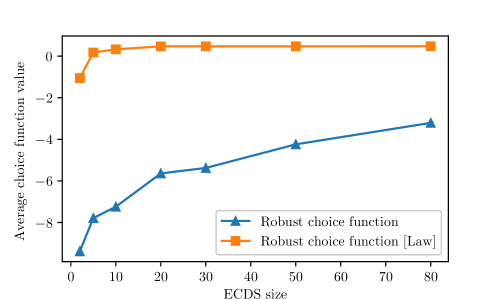
Figure 2: Normalized RCF value with increasing ECDS size

We also illustrate the relationship between the robust optimal portfolio weights and the number of ECDS pairs. In this experiment, we choose the batch size to be $M=5$. The optimal portfolio always consists of a mixture of only Asset 1, Asset 4, and Asset 5.

In Figure 3, the result for the basic case without [Law] is shown in the left plot and the result with [Law] is shown in the right plot. The weight on Asset 5 is at the top (purple area), the weight on Asset 4 is in the middle (red area), and the weight on Asset 1 is on the bottom (blue area). The true optimal solution under the perceived choice function is to put all weight on Asset 5. We see that when there are more than five ECDS pairs, the law invariant model already reaches a stable solution that matches the “true” optimal solution under the perceived choice function. The model without [Law] reaches a stable solution once there are more than twenty ECDS pairs, with a small optimality gap.

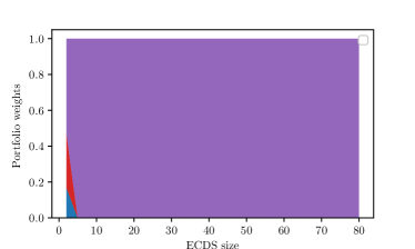
Figure 3: Robust optimal solution for portfolio optimization in the base case (left) and the law-invariant case (right)

In the next experiment, we compare the perceived choice function value of the optimal solutions of four different models: our RCF (base and law invariant cases), expected return, and the perceived choice function itself. In each experimental run, we randomly select twenty assets from the pool (which consists of all 212 assets) as the batch (the selected assets over which we do PRO). Then, for each instance, we calculate the perceived choice function values of the solutions proposed by PRO with and without [Law], expected return maximization, and perceived choice function maximization. We conduct 500 experimental runs and then calculate the average of the optimal choice function values, which serve as a measure of the performance of PRO. They represent how good the DM feels about the solutions proposed by an advisor using PRO.

In Figure 4, we see that the performance of PRO improves as the size of the ECDS increases. We also note that the law-invariant RCF always outperforms our basic RCF without [Law]. We conjecture that this is because the perceived choice function (certainty equivalent) is actually law-invariant. Finally, we see that the law-invariant RCF is fairly close to ground truth once the size of the ECDS is greater than ten. In this case, enforcing [Law] greatly improves the fidelity of our PRO approach with respect to the ground truth.

Figure 4: Performance of the portfolios proposed by different methods

8.2 Capital allocation

Our next application is to scenario dependent capital allocation for a financial institution consisting of sub-units $n\in[N]$ for $N\geq 1$. The overall financial institution is represented by the random vector

$$X=(X_{1}(\omega),X_{2}(\omega),\ldots,\,X_{N}(\omega))_{\omega\in\Omega},$$

where we interpret each $X_{n}$ as the random revenue of sub-unit $n\in[N]$. Define

$$\mathcal{Z}=\left\{Z\in\mathcal{L}^{N}:\sum^{N}_{n=1}Z_{n}(\omega)\leq B,\,Z(\omega)\geq 0,\,\forall\omega\in\Omega\right\},$$

to be the set of admissible scenario-dependent financial recourse decisions subject to a budget constraint $B>0$. Our problem is to maximize the RCF subject to the available budget:

$$\max_{Z\in\mathcal{Z}}\psi_{\mathscr{R}}(X+Z).$$ (31)

We suppose there is a systematic risk factor $\varphi\sim Normal(0,\,2\%)$ common to all sub-units and an idiosyncratic risk factor $\xi_{n}\sim Normal(n\times 3\%,\,n\times 2.5\%)$ specific to sub-unit $n\in[N]$. We then set the return to be $X_{n}=10(\varphi+\xi_{n})$ (this is similar to the experimental setup in Esfahani and Kuhn (2018)). To construct ECDS for our experiments, we randomly generate samples of financial returns according to this setup. The DM’s preference for each pair of assets is determined by using the perceived choice function in Eq. (29). We randomly select the weight vector $w$ uniformly from the unit simplex, and set the budget to be $B=0.5$.

8.2.1 Scalability

To test the scalability of our sorting algorithm, we model an institution with $N=20$ sub-units on $T=20$ scenarios. The run times of our sorting algorithm and Gurobi are presented in Table 2. As for the portfolio problem, here we also do comparisons among five groups where the ECDS is randomly generated for each group. We see the difference in required computation time between our sorting algorithm and Gurobi is more pronounced in this application compared to the portfolio optimization problem.

We next consider scalability of our law invariant sorting algorithm. Table 3 suggests that the law invariant sorting algorithm is highly scalable in terms of the number of scenarios and the number of attributes. Note that the most rapid growth in run time is in the number of ECDS pairs. This result is not surprising since the complexity of our sorting algorithm grows quadratically in the number of ECDS pairs by Theorem 4.7.

			ECDS Pairs
Method	Group		10	20	30	40	50
Sorting	1		15.6s	97s	364s	841s	1631s
	2		13.2s	107s	350s	826s	1539s
	3		12.5s	99s	326s	808s	1483s
	4		12.6s	107s	342s	823s	1651s
	5		13s	97s	337s	781s	1545s
	Average		13.38s	101.4s	343.8s	815.8s	1569.8s
MILP	1		7.16s	56.13s	185.78s	3728.40s	22109.66s
	2		4.64s	59.92s	254.80s	5312.21s	31019.20s
	3		6.47s	90.27s	450.12s	6560.72s	38534.88s
	4		5.30s	71.62s	387.61s	5666.33s	36112.33s
	5		5.18s	38.9s	278.50s	5449.45s	32334.57s
	Average		5.75s	69.48s	296.90	5343.42s	32022.13s

Table 2: Scalability of the sorting algorithm for capital allocation

			ECDS Pairs
Settings	Group		1	2	5	10	20	50	80
20 Scen, 20 Attr	1		52.9ms	437ms	7.19s	52.4s	506s	6715s	28284s
	2		47.5ms	420ms	7.12s	52.8s	507s	6822s	30111s
	3		52ms	445ms	7.28s	52.5s	508s	6720s	27765s
	4		50.2ms	440ms	7.2s	53s	511s	6669s	28202s
	5		51.8ms	444ms	7.22s	52.4s	512s	6733s	28116s
	Average		50.88ms	437.2ms	7.202s	52.62s	508.8s	6731.8s	28495.6s
			Number of Scenarios
Settings	Group		5	10	15	20	50	100	200
10 Pairs, 20 Attr	1		6.64s	17s	33.4s	54.3s	274s	1141s	4532s
	2		6.75s	17.1s	33.2s	55.1s	274s	1222s	4605s
	3		6.58s	16.8s	33.3s	52.8s	280s	1088s	4520s
	4		6.32s	17.9s	33.6s	54.2s	269s	1050s	4330s
	5		6.67s	16.9s	33.8s	55s	271s	1150s	4567s
	Average		6.592ms	17.14s	33.46s	54.28s	273.6s	1130.2s	4510.8s
			Number of Attributes
Settings	Group		5	10	15	20	50	100	200
10 Pairs, 20 Scen	1		21s	31s	40.9s	51.5s	124s	246s	480s
	2		20s	31s	40.6s	51.2s	122s	244s	484s
	3		19s	31s	40.7s	51.6s	123s	248s	482s
	4		20s	30s	41.2s	52.2s	126s	250s	480s
	5		21s	32s	41s	51.8s	124s	246s	481s
	Average		20.2s	31s	40.88s	51.66s	123.8s	246.8s	481.4s

Table 3: Scalability of the sorting algorithm for capital allocation (law-invariant case)

We also investigate the scalability of the binary search algorithm for the capital allocation problem (which takes the optimal solution of the value problem as input). Table 4 shows that the algorithm is highly scalable in terms of the size of the ECDS, the number of attributes, and the number of scenarios.

			ECDS Pairs
Settings	Group		1	2	5	10	20	50	80
20 Scen, 20 Attr	1		576ms	867ms	1.21s	1.46s	1.84s	2.38s	4.56s
	2		532ms	902ms	1.17s	1.51s	1.82s	2.32s	4.62s
	3		555ms	855ms	1.15s	1.45s	1.81s	2.4s	4.88s
	4		546ms	832ms	1.22s	1.47s	1.85s	2.33s	4.67s
	5		612ms	841ms	1.23s	1.46s	1.9s	2.35s	4.51s
	Average		564.2ms	859.4ms	1.196s	1.47s	1.844s	2.356s	4.648s
			Number of Scenarios
Settings	Group		5	10	15	20	50	100	200
10 Pairs, 20 Attr	1		153ms	414ms	1.02s	1.46s	8.8s	40s	181s
	2		115ms	414ms	924ms	1.36s	9.79s	35s	177s
	3		130ms	376ms	919ms	1.32s	10s	38s	190s
	4		119ms	427ms	917ms	1.33s	7.88s	42s	176s
	5		131ms	425ms	922ms	1.42s	9.47s	40s	183s
	Average		129.6ms	417.2ms	940.4ms	1.378s	9.188s	39s	181.4s
			Number of Attributes
Settings	Group		5	10	15	20	50	100	200
10 Pairs, 20 Scen	1		402ms	745ms	1.42s	1.6s	4.56	9.42s	18.5s
	2		398ms	740ms	1.38s	1.55s	4.6s	9.44s	18.7s
	3		396ms	740ms	1.37s	1.56s	4.61s	9.45s	19s
	4		408ms	750ms	1.45s	1.61s	4.6s	9.39s	18.8s
	5		405ms	744ms	1.44s	1.61s	4.56s	9.4s	18.9s
	Average		401.8ms	743.8ms	1.412s	1.586s	4.586s	9.42s	18.78s

Table 4: Scalability of the binary search algorithm for capital allocation

8.2.2 Effectiveness of robust framework

We want to see how well our RCF approximates the perceived choice function for different sizes of ECDS, and we also want to see how the PRO solutions compare with the ground truth solution. We first test the RCF value with increasing ECDS size. We randomly sample 500 financial positions $X$, calculate the RCF values $\psi_{\mathscr{R}\left(\mathcal{E}\right)}(X)$ ($\psi_{\mathscr{R}_{L}\left(\mathcal{E}\right)}(X)$) of each financial position $X$, and then calculate the average. We run this experiment for several ECDS with different sizes. Figure 5 reports the average RCF value when there are $T=4$ scenarios and $N=4$ sub-units. This figure shows the speed at which the RCF “converges” as more pairwise comparison data is given. As we saw earlier for the portfolio application, this experiment indicates that if [Law] is enforced then only a few comparisons (possibly fewer than ten ECDS pairs) are needed to make robust decisions of high quality.

Figure 5: RCF value with increasing ECDS size

The final experiment tests the performance of the capital allocation plans proposed by different models: RCF (base and law invariant), expected return, and the perceived choice function. For the expected return, we use the uniform weight $w_{0}=(\frac{1}{N},\ldots,\frac{1}{N})$ as our guess because the ground truth is unknown. In each experimental run, we randomly generate a financial position. Then, for each model, we calculate the perceived choice function values of the allocation plans proposed by these models. We conduct 500 experimental runs and calculate the average, the results are shown in Figure 6.

Similar to the portfolio application, law-invariant PRO better matches the law invariant perceived choice function. Second, the performance of both PRO and PRO with [Law] improves as we increase the size of the ECDS. However, we see that the convergence rate of law-invariant PRO is slower here than it was in the portfolio problem. One possible explanation is that, in the multi-attribute case, enforcing [Law] only facilitates learning among different scenarios, but not learning among different attributes. We hypothesize that more elicited pairs are needed to achieve the same performance for multi-attribute PRO compared to the single-attribute case.

Figure 6: Performance of the allocation plans proposed by different methods

9 Conclusions

This paper has put forward a robust choice model that supports: (i) quasi-concavity; (ii) law invariance; and (iii) multi-attribute prospects. Both concavity and quasi-concavity correspond to diversification-favoring behavior, but quasi-concavity is easier to check for a new DM compared to the stronger property of concavity. Our model also supports multi-attribute problems and it avoids the need to assign artificial weights to each attribute to do ranking and optimization.

We show that we can evaluate our RCF efficiently. As our main methodological contribution, we show how to determine the values of the RCF and construct its acceptance sets by solving a sequence of linear programming problems. Then, we show how to efficiently solve our PRO problem by solving a sequence of convex optimization problems. Even though the property of quasi-concavity introduces non-convexity into our model, we only ever have to solve a polynomial number of linear/convex optimization problems.

Our numerical experiments show that our method has practical computational complexity in terms of the number of scenarios, attributes, and the size of the ECDS - even in the law invariant case. The greatest computational expenditure is on the value problem. Once the value problem is solved, the PRO problem can generally be solved quickly.

Appendix A Additional material for Section 2

A.1 Proof of Proposition 2.3 (Lipschitz continuity of RCF)

Part (i). We will verify that all of our axiomatic properties are preserved by the infimum. For [Mon], let $\vec{X}\leq\vec{Y}$ then

$$\psi_{\mathscr{R}}(\vec{X})=\inf_{\phi\in\mathscr{R}}\phi(\vec{X})\leq\inf_{\phi\in\mathscr{R}}\phi(\vec{Y})=\psi_{\mathscr{R}}(\vec{Y}).$$

For [QCo], let $\vec{X},\,\vec{Y}\in\mathbb{R}^{TN}$ and $\lambda\in[0,1]$, then

$$\psi_{\mathscr{R}}(\lambda\,\vec{X}+(1-\lambda)\vec{Y})=\inf_{\phi\in\mathscr{R}}\phi(\lambda\,\vec{X}+(1-\lambda)\vec{Y})\geq\inf_{\phi\in\mathscr{R}}\min\{\phi(\vec{X}),\,\phi(\vec{Y})\}\geq\min\{\psi_{\mathscr{R}}(\vec{X}),\,\psi_{\mathscr{R}}(\vec{Y})\}.$$

Similarly, [Usc] and [Nor] are both preserved by the infimum.

Since all $\phi\in\mathscr{R}$ are $C-$Lipschitz continuous, we have

$$|\psi_{\mathscr{R}}(\vec{X})-\psi_{\mathscr{R}}(\vec{Y})|\leq\sup_{\phi\in\mathscr{R}}|\phi(\vec{X})-\phi(\vec{Y})|\leq C\,\|\vec{X}-\vec{Y}\|,$$

using the inequality

$$|\max_{x\in\mathcal{X}}f(x)-\max_{x\in\mathcal{X}}g(x)|\leq\max_{x\in\mathcal{X}}|f(x)-g(x)|,$$

which holds for any set $\mathcal{X}$ and functions $f:\mathcal{X}\rightarrow\mathbb{R}$ and $g:\mathcal{X}\rightarrow\mathbb{R}$.

For [Law], suppose $X=_{D}Y$, then

$$\psi_{\mathscr{R}}(\vec{X})=\inf_{\phi\in\mathscr{R}}\phi(\vec{X})=\inf_{\phi\in\mathscr{R}}\phi(\vec{Y})=\psi_{\mathscr{R}}(\vec{Y}).$$

Finally, to verify [Eli], fix $k=1,\ldots,K$ and $\epsilon>0$. Let $\phi\in\mathscr{R}$ be such that $\psi_{\mathscr{R}}(\vec{W}_{k})\geq\phi(\vec{W}_{k})-\epsilon$. Then we have $\psi_{\mathscr{R}}(\vec{W}_{k})\geq\phi(\vec{Y}_{k})-\epsilon\geq\psi_{\mathscr{R}}(\vec{Y}_{k})-\epsilon$ using $\phi(\vec{W}_{k})\geq\phi(\vec{Y}_{k})$ for all $\phi\in\mathscr{R}$, and $\phi(\vec{Y}_{k})\geq\psi_{\mathscr{R}}(\vec{Y}_{k})$. Since $\epsilon$ was arbitrary, the desired result follows.

To conclude, for any $\vec{X}\in\mathbb{R}^{TN}$, we have

$$|\psi_{\mathscr{R}}(\vec{X})|\leq|\psi_{\mathscr{R}}(\vec{W}_{0})|+L\,\|\vec{W}_{0}-\vec{X}\|\leq C\,\|\vec{W}_{0}-\vec{X}\|<\infty,$$

by [Nor] and [Lip] (which are both preserved by the infimum) which means that $\psi_{\mathscr{R}}(\vec{X})$ is well-defined and finite-valued for any $\vec{X}\in\mathbb{R}^{TN}$.

Part (ii). For the rest of this proof, we explicitly indicate the dependence of our ambiguity sets on the Lipschitz constant $C$:

$$\mathscr{R}(C,\,\mathcal{E}):=\mathfrak{R}\cap\mathscr{R}_{\text{Nor}}(\vec{W}_{0})\cap\mathscr{R}_{\text{Lip}}(C)\cap\mathscr{R}_{\text{Eli}}(\mathcal{E}),$$

and

$$\mathscr{R}_{L}(C,\,\mathcal{E}):=\mathfrak{R}\cap\mathscr{R}_{\text{Nor}}(\vec{W}_{0})\cap\mathscr{R}_{\text{Lip}}(C)\cap\mathscr{R}_{\text{Law}}\cap\mathscr{R}_{\text{Eli}}(\mathcal{E}).$$

Now, for $\mathscr{R}(C)\in\{\mathscr{R}(C,\,\mathcal{E}),\,\mathscr{R}_{L}(C,\,\mathcal{E})\}$, we will establish that $\mathscr{R}(C)=C\,\mathscr{R}(1)$ and $\psi_{\mathscr{R}(C)}=C\,\psi_{\mathscr{R}(1)}$. It would follow that $\psi_{\mathscr{R}(C)}$ is just a positive linear transformation of $\psi_{\mathscr{R}(1)}$, and so the induced preference relations must be equivalent.

For any $C\geq 0$, we have $\psi_{\mathscr{R}(C)}=C\,\psi_{\mathscr{R}(1)}$, where $\mathscr{R}(1)$ corresponds to normalized Lipschitz functions with modulus $1$. To establish this statement, we show that $\mathscr{R}(C)=C\,\mathscr{R}(1)$. Choose any $\phi\in\mathscr{R}(1)$, then $C\,\phi\in\mathscr{R}(C)$ since $C\,\phi$ is $C-$Lipschitz and so it follows that $C\,\mathscr{R}(1)\subset\mathscr{R}(C)$. Now choose any $\phi\in\mathscr{R}(C)$. Then $\phi=C(1/C)\phi$ and $(1/C)\phi\in\mathscr{R}(1)$ since $\phi$ is $C-$Lipschitz, and so it follows that $\mathscr{R}(C)\subset C\,\mathscr{R}(1)$.

Appendix B Additional material for Section 3 (preference robust optimization)

B.1 Results on quasi-convex analysis

Here we present two key technical results that allow us to obtain tractable formulations for our RCF. We begin with a technical lemma that characterizes Lipschitz continuous quasi-concave functions in terms of their upper subgradients, defined as follows.

Definition B.1.

Let $f:\mathbb{R}^{d}\rightarrow\mathbb{R}$ and fix $x\in\mathbb{R}^{d}$. Then $s\in\mathbb{R}^{d}$ is an upper subgradient of $f$ at $x$ if $h_{x}(y;s):=f(x)+\max\{\langle s,\,y-x\rangle,\,0\}\geq f(y)$ for all $y\in\text{dom}(f)$. The set of all upper subgradients of $f$ at $x$ is called the upper subdifferential and is denoted by $\partial^{+}f(x)$.

Lemma B.1.

Let $\|\cdot\|$ be a norm on $\mathbb{R}^{d}$ and let $\|\cdot\|_{*}$ be its dual norm. A quasi-concave function $f:\mathbb{R}^{d}\rightarrow\mathbb{R}$ is $C-$Lipschitz with respect to $\|\cdot\|$ if and only if for every $x\in\mathbb{R}^{d}$, there exists an upper subgradient $a\in\partial^{+}f(x)$ such that $\|a\|_{*}\leq C$.

Proof.

See Plastria (1985) for the proof of the case for the Euclidean norm $\|\cdot\|=\|\cdot\|_{2}$. This proof can be generalized to any norm using the general Cauchy-Schwarz inequality $\langle x,y\rangle\leq\|x\|_{*}\|y\|$ for all $x,\,y\in\mathbb{R}^{d}$.

Suppose that for every $x\in\mathbb{R}^{d}$, there exists an upper subgradient $a\in\partial^{+}f(x)$ such that $\|a\|_{*}\leq C$. Let $x,y\in\mathbb{R}^{d}$ and assume WLOG that $f(y)\geq f(x)$. For the case where $f(y)=f(x)$, $f(y)-f(x)\leq C\|y-x\|$ follows trivially. For the case where $f(y)>f(x)$, we have $0<f(y)-f(x)\leq\langle a,y-x\rangle\leq\|a\|_{*}\|y-x\|\leq C\|y-x\|$.

For the other direction, suppose that $f$ is $C-$Lipschitz and quasi-concave. For any $x\in\mathbb{R}^{d}$, let $S$ be the upper level set of $f$ at $x$, which is convex by quasi-concavity of $f$. Then, there exists a separating hyperplane for $x$ and $S$. Specifically, there exists $a_{0}$ with $\|a_{0}\|=1$ such that $\langle y-x,a_{0}\rangle\geq 0$ for all $y\in S$.

Let $a=C\,a_{0}/\|a_{0}\|_{*}$, we will prove that $a$ is an upper-subgradient of $f$. Let $e_{0}\in\arg\max_{\|e\|=1}\langle e,a\rangle$, then we have $\langle e_{0},a\rangle=\|a\|_{*}$ by definition of the dual norm. Now fix any $y\in S$, and let $y^{\prime}$ lie on the separating hyperplane (i.e., $\langle a_{0},y^{\prime}-x\rangle=0$) such that $y-y^{\prime}=\|y-y^{\prime}\|\,e_{0}$. Then, we have

$$\langle a,y-x\rangle=\langle a,y-y^{\prime}\rangle=\langle a,e_{0}\rangle\|y-y^{\prime}\|=\|a\|_{*}\|y-y^{\prime}\|=C\|y-y^{\prime}\|.$$ (32)

On the other hand, we have $f(y^{\prime})\leq f(x)$ since $y^{\prime}$ lies on the separating hyperplane. By Lipschitz continuity of $f$, it follows that

$$f(y)-f(x)\leq f(y)-f(y^{\prime})\leq C\|y-y^{\prime}\|.$$ (33)

Combining (32) and (33), we see that $f(y)-f(x)\leq\langle a,y-x\rangle$ for all $y\in S$. Since $\|a\|_{*}=C$ by construction, the desired conclusion follows. ∎

We now present another technical lemma that characterizes quasi-concave functions via the class of kinked majorants.

Lemma B.2.

Let $f:\mathbb{R}^{d}\rightarrow\mathbb{R}$. The following assertions hold.

• Suppose that $f$ has a kinked majorant everywhere in its domain. Then, $f$ is quasi-concave, upper semi-continuous, and has a representation

  $$f\left(x\right)=\inf_{j\in\mathcal{J}}h_{j}\left(x\right),\,\forall x\in\text{dom}\,f,$$ (34)

  where $\mathcal{J}$ is a (possibly infinite) index set and $h_{j}\left(x\right)=\max\left\{\langle a_{j},\,x-x_{j}\rangle,\,0\right\}+b_{j}$ for all $j\in\mathcal{J}$ with constants $a_{j}\in\mathbb{R}^{d}$, $x_{j}\in\mathbb{R}^{d}$, and $b_{j}\in\mathbb{R}$.

• Suppose $f$ is quasi-concave and $C-$Lipschitz continuous with respect to $\|\cdot\|_{\infty}$, then $f$ has a representation (34) with $\|a_{j}\|_{1}\leq C$ for all $j\in\mathcal{J}$.

• If $f$ has a representation (34), then it is quasi-concave. Moreover, if $a_{j}\geq 0$ for all $j\in\mathcal{J}$, then $f$ is non-decreasing. Conversely, if $f$ is non-decreasing and quasi-concave, then there exists a set of kinked majorants $\{h_{j}\}$ with $a_{j}\geq 0$ such that representation (34) holds.

• For any finite set $\Theta\subset\mathbb{R}^{d}$ and values $\left\{v_{\theta}\right\}_{\theta\in\Theta}\subset\mathbb{R}$, $\hat{f}\text{ : }\mathbb{R}^{d}\rightarrow\mathbb{R}$ defined by

  $$\hat{f}\left(x\right):=\inf_{a,\,b}\quad b$$

  s.t. $$\max\left\{\langle a,\,\theta-x\rangle,\,0\right\}+b\geq v_{\theta},\,\forall\theta\in\Theta,$$ (35)

  $$\|a\|_{1}\leq C,$$

  is quasi-concave. Furthermore, the graph of $\hat{f}$ is the (pointwise) minimum of all $C-$Lipschitz quasi-concave majorants of $\left\{\left(\theta,\,v_{\theta}\right)\text{ : }\theta\in\Theta\right\}$.

The proof is covered by (Haskell et al., 2022, Theorem 1). Note that $\hat{f}$ in Eq. ((iv)) is a specific example of the more general representation $f$ in Eq. (34).

B.2 Proof of Theorem 3.1 (disjunctive programming formulation)

Lemma B.3.

Problem (2) has an optimal solution.

Proof.

First, we note that Problem (2) always has a feasible solution since we can choose $v=0$ and $s=0$. Next, we note that feasible $s=(s_{\theta})$ are bounded by Constraints (2g) and (2g) (Lipschitz continuity and monotonicity).

We will also show that feasible $v=(v_{\theta})$ are bounded. First note that we can assume $v_{X}\leq 0$ since $v=0$ and $s=0$ is a feasible solution with objective value $v_{X}=0$. By Constraint (2g) (normalization), and the choice of $\vec{W}_{0}$, we have $v_{\theta}\leq 0$ for all $\theta\in\Theta$. Then, by Constraints (2g) (quasi-concavity) and (2g) (Lipschitz continuity), for all $\theta\in\Theta$ with $\theta\neq\vec{W}_{0}$, we must have $v_{\theta}\geq-C\|\theta-\vec{W}_{0}\|$. Similarly, by Constraints (2g) and (2g) we must have $v_{X}\geq-C\|\vec{X}-\vec{W}_{0}\|$. It then follows that $|v_{\theta}|\leq C\|\theta-\vec{W}_{0}\|$ for all $\theta\in\Theta$ and $|v_{X}|\leq C\|\vec{X}-\vec{W}_{0}\|$, and so feasible $v=(v_{\theta})_{\theta\in\Theta}$ are bounded.

We have established that Problem (2) is equivalent to minimization of a continuous function over a compact set, and so its minimum is attained and an optimal solution exists by the Weierstrass theorem. ∎

B.3 Proof of Proposition 3.2

First suppose $\phi\in\mathfrak{R}$ satisfies $\phi(\theta)=v_{\theta}$ for all $\theta\in\Theta$. Since $\phi$ satisfies [QCo], by Lemma B.2 Part (ii) we have

$$\phi(\vec{X})=\inf_{j\in\mathcal{J}}h_{j}(\vec{X}),\,\forall\vec{X}\in\mathbb{R}^{TN},$$

where $\{h_{j}\}_{j\in\mathcal{J}}$ is a set of kinked majorants. Then, for each $\theta\in\Theta$ we have $\phi(\theta)=v_{\theta}=\inf_{j\in\mathcal{J}}h_{j}(\theta)\leq h_{j^{*}(\theta)}(\theta)$ for any choice of $j^{*}(\theta)\in\mathcal{J}$, and $h_{j^{*}(\theta)}(\theta^{\prime})\geq\inf_{j\in\mathcal{J}}h_{j}(\theta^{\prime})=v_{\theta^{\prime}}$ for all $\theta^{\prime}\in\Theta$ with $\theta^{\prime}\neq\theta$.

For the other direction, suppose we have kinked majorants $h_{\theta}$ of $\phi$ at all $\theta\in\Theta$. Consider the function $\psi(\cdot)=\min_{\theta\in\Theta}h_{\theta}(\cdot;s_{\theta})$, which is defined by the pointwise minimum of all such $h_{\theta}$. We see that $\psi\in\mathscr{R}_{\text{QCo}}\cap\mathscr{R}_{\text{Lip}}(C)$ since [Mon], [QCo], and [Lip] are satisfied by all $h_{\theta}$ and are preserved by the infimum. Furthermore, $\psi(\theta)=v_{\theta}$ for all $\theta\in\Theta$, so we have successfully constructed $\psi\in\mathfrak{R}$ that exactly attains the desired values on $\Theta$.

B.4 Proof of Theorem 3.3 (two-stage decomposition)

For each $\theta\in\Theta$, we introduce the problem:

$$({\mathscr{P}}_{\theta})\qquad\min_{v,\,s}\, v_{\theta}$$ (36a)

s.t. $$v_{\theta}+\max\left\{\langle s_{\theta},\,\theta^{\prime}-\theta\rangle,\,0\right\}\geq v_{\theta^{\prime}},\quad\forall\left(\theta,\,\theta^{\prime}\right)\in\widehat{\Theta},$$ (36e)

$$s_{\theta}\geq 0,\,\|s_{\theta}\|_{1}\leq C,\quad\forall\theta\in\Theta,$$

$$v_{\theta}\geq v_{\theta^{\prime}},\quad\forall\left(\theta,\,\theta^{\prime}\right)\in\mathcal{E},$$

$$v_{W_{0}}=0,$$

which just minimizes the value $v_{\theta}$ corresponding to the RCF at $\theta$.

Lemma B.4.

Problem $\mathscr{P}_{\theta}$ has an optimal solution for all $\theta\in\Theta$.

Proof.

First, we note that Problem $\mathscr{P}_{\theta}$ is always feasible since we can choose $v=0$ and $s=0$. Next, we see that feasible $s$ are bounded by Constraint (36e) (Lipschitz continuity and monotonicity). We will also show that feasible $v$ are bounded.

By Constraint (36e) (normalization), and the choice of $\vec{W}_{0}$, we have $v_{\theta}\leq 0$ for all $\theta\in\Theta$. Then, by Constraint (36e) (quasi-concavity) and Constraint (36e), for all $\theta\in\Theta$ with $\theta\neq\vec{W}_{0}$, we must have $v_{\theta}\geq-L\|\theta-\vec{W}_{0}\|$. It then follows that $|v_{\theta}|\leq C\|\theta-\vec{W}_{0}\|$ for all $\theta\in\Theta$, and so feasible $v$ are bounded.

Problem $\mathscr{P}_{\theta}$ is then minimizing a continuous function over a compact set, and so its minimum is attained and an optimal solution exists by the Weierstrass theorem. ∎

Next, we fix $\vec{X}\in\mathbb{R}^{TN}$ and connect evaluation of $\psi_{\mathscr{R}(\mathcal{E})}(\vec{X})$ to the interpolation problem. In particular, evaluation of $\psi_{\mathscr{R}(\mathcal{E})}(\vec{X})$ can be thought of as minimizing $\phi(\vec{X})$ over the majorants $\phi\in\mathfrak{R}$ of $\psi_{\mathscr{R}(\mathcal{E})}$ at $\vec{X}$, as the following lemma shows.

Lemma B.5.

For all $\vec{X}\in\mathbb{R}^{TN}$, we have

$$\psi_{\mathscr{R}(\mathcal{E})}(\vec{X})=\inf_{\phi\in\mathscr{R}_{\text{QCo}}\cap\mathscr{R}_{\text{Lip}}(C)}\{\phi(\vec{X}):\phi(\theta)\geq\psi_{\mathscr{R}(\mathcal{E})}(\theta),\,\forall\theta\in\Theta\}.$$

Proof.

Define

$$\tilde{\psi}(\vec{X}):=\inf_{\phi\in\mathscr{R}_{\text{QCo}}\cap\mathscr{R}_{\text{Lip}}(C)}\{\phi(\vec{X}):\phi(\theta)\geq\psi_{\mathscr{R}(\mathcal{E})}(\theta),\,\forall\theta\in\Theta\}.$$

We will establish equivalence between $\psi_{\mathscr{R}(\mathcal{E})}$ and $\tilde{\psi}$. First, it is immediate that $\tilde{\psi}\leq\psi_{\mathscr{R}(\mathcal{E})}$, since $\tilde{\psi}$ is only required to majorize $\psi_{\mathscr{R}(\mathcal{E})}$ on $\Theta$ (and not on all of $\mathbb{R}^{TN}$).

For the other direction, note that the set

$$\{\phi\in\mathscr{R}_{\text{QCo}}\cap\mathscr{R}_{\text{Lip}}(C):\phi(\theta)\geq\psi_{\mathscr{R}(\mathcal{E})}(\theta),\,\forall\theta\in\Theta\}$$

is closed under minimization by the same argument as Proposition 2.3. In particular, for each $\theta\in\Theta$, we can choose a function $h_{\theta}\in\mathscr{R}_{\text{QCo}}\cap\mathscr{R}_{\text{Lip}}(C)$ such that $h_{\theta}(\theta)=\psi_{\mathscr{R}(\mathcal{E})}(\theta)$ and $h_{\theta}(\theta^{\prime})\geq\psi_{\mathscr{R}(\mathcal{E})}(\theta^{\prime})$ for all $\theta^{\prime}\in\Theta$. Then, we can define the function $\phi(\cdot)=\min_{\theta\in\Theta}h_{\theta}(\cdot)$ which satisfies $\phi(\theta)=\psi_{\mathscr{R}(\mathcal{E})}(\theta)$ for all $\theta\in\Theta$ (i.e., equality is attained at all $\theta\in\Theta$. We then obtain the equivalent form:

$$\tilde{\psi}(\vec{X})=\inf_{\phi\in\mathscr{R}_{\text{QCo}}\cap\mathscr{R}_{\text{Lip}}(C)}\{\phi(\vec{X}):\phi(\theta)=\psi_{\mathscr{R}(\mathcal{E})}(\theta),\,\forall\theta\in\Theta\}.$$

By this representation of $\tilde{\psi}$, we see that $\tilde{\psi}$ satisfies [Nor], [Lip], and [Eli] and thus $\tilde{\psi}\in\mathscr{R}(\mathcal{E})$. It follows that $\psi_{\mathscr{R}(\mathcal{E})}\leq\tilde{\psi}$ must also hold, completing the argument. ∎

Proof of Theorem 3.3.

For each $\theta\in\Theta$, $\mathscr{P}_{\theta}$ has an optimal solution $(v^{*}(\theta),s^{*}(\theta))$, and we can define a corresponding kinked majorant $h_{\theta}(\cdot;v^{*}(\theta),s^{*}(\theta))$ via

$$h_{\theta}(\vec{X};v^{*}(\theta),s^{*}(\theta))=v^{*}(\theta)+\max\{0,\langle s^{*}(\theta),\vec{X}-\theta\rangle\},\,\forall\vec{X}\in\mathbb{R}^{TN}.$$

We then define $\psi^{*}$ via

$$\psi^{*}(\vec{X})=\min_{\theta\in\theta}h_{\theta}(\vec{X};v^{*}(\theta),s^{*}(\theta)),\,\forall\vec{X}\in\mathbb{R}^{TN}.$$

By Proposition 2.3, the set $\mathscr{R}\left(\mathcal{E}\right)$ is closed under minimization, so we must have $\psi^{*}\in\mathscr{R}\left(\mathcal{E}\right)$ as well. It follows that $\psi_{\mathscr{R}\left(\mathcal{E}\right)}(\theta)\leq\psi^{*}(\theta)$ for all $\theta\in\Theta$ by definition of $\psi_{\mathscr{R}\left(\mathcal{E}\right)}$. But, for each $\theta\in\Theta$, we have $\psi^{*}(\theta)=h_{\theta}^{*}(\theta;v^{*}(\theta),s^{*}(\theta))\leq\phi(\theta)$ for all $\phi\in\mathscr{R}\left(\mathcal{E}\right)$. Subsequently

$$\sum_{\theta\in\Theta}\psi^{\ast}\left(\theta\right)=\sum_{\theta\in\Theta}h_{\theta}\left(\theta;v^{*}(\theta),s^{*}(\theta)\right)\leq\sum_{\theta\in\Theta}\phi(\theta),$$

for any $\phi\in\mathscr{R}(\mathcal{E})$. It follows that $\psi^{*}(\theta)=\psi_{\mathscr{R}(\mathcal{E})}(\theta)$ must hold for all $\theta\in\Theta$ since $\psi_{\mathscr{R}(\mathcal{E})}\in\mathscr{R}(\mathcal{E})$, and we have the lower bound $\sum_{\theta\in\Theta}h_{\theta}\left(\theta;v^{*}(\theta),s^{*}(\theta)\right)$ on the optimal value of $\mathscr{P}$. Since, for all $\theta\in\Theta$, $\phi(\theta)\geq h_{\theta}\left(\theta;v^{*}(\theta),s^{*}(\theta)\right)$, this lower bound is only attained for $\phi\in\mathfrak{R}$ such that $\phi(\theta)=h_{\theta}\left(\theta;v^{*}(\theta),s^{*}(\theta)\right)$ for all $\theta\in\Theta$. Thus, the optimal solution of $\mathscr{P}$ has the unique values $h_{\theta}\left(\theta;v^{*}(\theta),s^{*}(\theta)\right)=\psi_{\mathscr{R}(\mathcal{E})}(\theta)$ for all $\theta\in\Theta$.

Next, by Lemma B.5 we have

$$\psi_{\mathscr{R}(\mathcal{E})}(\vec{X})=\inf_{\phi\in\mathscr{R}_{\text{QCo}}\cap\mathscr{R}_{\text{Lip}}(C)}\{\phi(\vec{X}):\phi(\theta)\geq\psi_{\mathscr{R}(\mathcal{E})}(\theta),\,\forall\theta\in\Theta\}.$$

Since $v^{*}$ is the optimal solution of $\mathscr{P}$, for any $\vec{X}\in\mathbb{R}^{TN}$ we have the equality

$$\psi_{\mathscr{R}(\mathcal{E})}(\vec{X})=\min_{v}\left\{v\in\mathbb{R}:\phi(\vec{X})=v,\,\phi\in\mathscr{R}_{\text{QCo}}\cap\mathscr{R}_{\text{Lip}}(C),\,\phi(\theta)\geq v^{*}_{\theta},\,\forall\theta\in\Theta\right\}.$$

Then, $\psi_{\mathscr{R}\left(\mathcal{E}\right)}(\vec{X})=\textsf{val}(\mathscr{P}(\vec{X};\,v^{\ast}))$ for all $\vec{X}\in\mathbb{R}^{TN}$. ∎

B.5 Proof of Theorem 3.4 (sorting algorithm)

We will prove that the values $v=(v_{\theta})_{\theta\in\Theta}$ corresponding to $\mathcal{D}$ returned by Algorithm 1 are the optimal solution of $\mathscr{P}$ in the following three steps:

1. First, we verify that the candidate solution constructed in Algorithm 1 is well-defined.

2. Second, we verify that this candidate solution gives a lower bound on the optimal solution of $\mathscr{P}$.

3. Finally, we verify that this candidate solution is also feasible for $\mathscr{P}$. Thus, it must be the (unique) optimal solution of $\mathscr{P}$.

Recall the disjunctive program $\mathscr{P}_{D}(\theta;\,\mathcal{D}_{j})$ defined in Eq. (8) that we use to compute the largest $\psi_{\mathscr{R}(\mathcal{E})}-$value in $\mathcal{D}\backslash\mathcal{D}_{j}$ for given $\mathcal{D}_{j}$. A modified version of Algorithm 1 follows (see Algorithm 4) that is based on solving a sequence of instances of $\mathscr{P}_{D}(\theta;\,\mathcal{D}_{j})$. Algorithm 4 is similar to Algorithm 1, except that it uses the optimal value of the disjunctive program $\mathscr{P}_{D}(\theta;\,\mathcal{D}_{j})$ in place of the predictor $\pi(\theta^{\prime};\,\mathcal{D}_{j})$ (which is a function of the optimal value of the linear program $\mathscr{P}_{LP}(\theta;\,\mathcal{D}_{j})$).

Initialization: ${\Theta}$, $j=1$, and $\mathcal{D}_{j}=\{\theta_{1},0\}$;

while $j<J$ do

        Choose $\theta_{j+1}\in\arg\max_{\theta\in{\cal D}\backslash\mathcal{D}_{j}}\textsf{val}(\mathscr{P}_{D}(\theta;\,\mathcal{D}_{j}))$, and set $v_{\theta_{j+1}}:=\textsf{val}(\mathscr{P}_{D}(\theta;\,\mathcal{D}_{j}))$;

       

       Update $\mathcal{D}_{j+1}:=\{\mathcal{D}_{j},(\theta_{j+1},v_{\theta_{j+1}})\}$, and set $j:=j+1$;

       

end while

return $\mathcal{D}:=\mathcal{D}_{J}$.

Algorithm 4 (Modified) sorting algorithm for the value problem

We pause to verify that the recursive construction of Algorithm 4 is well-defined.

Lemma B.6.

For all $j\in[J-1]$, $\textsf{val}(\mathscr{P}_{D}(\theta;\,\mathcal{D}_{j}))$ is finite.

Proof.

Since $\theta_{1}=\vec{W}_{0}$ has value $0$, and every $\theta\in\Theta$ is finite, the optimal value $\textsf{val}(\mathscr{P}_{D}(\theta;\,\mathcal{D}_{1}))$ is finite by the Lipschitz continuity constraint. By induction, every sorted prospect in $\mathcal{D}_{j}$ has finite value and so the optimal value $\textsf{val}(\mathscr{P}_{D}(\theta;\,\mathcal{D}_{j}))$ is also finite. ∎

Additionally, we verify that Algorithm 4 outputs a monotone decreasing sequence of values $\{v_{\theta_{j}}\}_{j\in[J]}$ in $\mathcal{D}$.

Lemma B.7.

If $1\leq i<k\leq J$, then $v_{\theta_{i}}\geq v_{\theta_{k}}$.

Proof.

For any $j\in[J-1]$, we prove $v_{\theta_{j}}\geq v_{\theta_{j+1}}$. Let $(\hat{v}_{\theta_{j+1}},\hat{s}_{\theta_{j+1}})$ denote the optimal solution of $\mathscr{P}_{D}(\theta_{j+1};\,\mathcal{D}_{j-1})$. Since

$$\theta_{j}\in\arg\max_{\theta\in\mathcal{D}\backslash\mathcal{D}_{j}}\textsf{val}(\mathscr{P}_{D}(\theta;\,\mathcal{D}_{j})),$$

we must have $v_{\theta_{j}}=\textsf{val}(\mathscr{P}_{D}(\theta_{j};\,\mathcal{D}_{j-1}))\geq\textsf{val}(\mathscr{P}_{D}(\theta_{j+1};\,\mathcal{D}_{j-1}))=\hat{v}_{\theta_{j+1}}$. Then, we see that $(v_{\theta_{j+1}},s_{\theta_{j+1}}):=(v_{\theta_{j}},\hat{s}_{\theta_{j+1}})$ is feasible for $\mathscr{P}_{D}(\theta_{j+1};\,\mathcal{D}_{j})$ since $(\hat{v}_{\theta_{j+1}},\hat{s}_{\theta_{j+1}})$ is feasible and $v_{\theta_{j}}\geq\hat{v}_{\theta_{j+1}}$. Thus, $\textsf{val}(\mathscr{P}_{D}(\theta_{j+1};\,\mathcal{D}_{j}))\leq v_{\theta_{j}}$ and we have $v_{\theta_{j}}\geq v_{\theta_{j+1}}$. ∎

Next we verify that the construction of Algorithm 4 is a lower bound on $\textsf{val}(\mathscr{P})$.

Lemma B.8.

For all $j\in[J-1]$, $\textsf{val}(\mathscr{P}_{D}(\theta;\,\mathcal{D}_{j}))\leq\psi_{\mathscr{R}\left(\mathcal{E}\right)}(\theta)$ for all $\theta\notin\mathcal{D}_{j}$.

Proof.

We prove this statement by induction starting with $\mathcal{D}_{1}=\{(\vec{W}_{0},0)\}$. We see $\textsf{val}(\mathscr{P}_{D}(\theta;\,\mathcal{D}_{1}))$ is a lower bound for $\psi_{\mathscr{R}\left(\mathcal{E}\right)}(\theta)$ for all $\theta\notin\mathcal{D}_{1}$ (this is automatic because $\mathscr{P}_{D}(\theta;\,\mathcal{D}_{1})$ has fewer constraints than Problem (2) which computes $\psi_{\mathscr{R}\left(\mathcal{E}\right)}(\theta)$ exactly). Proceeding inductively, if every $v_{\theta_{k}}$ in $\mathcal{D}_{j}$ is a lower bound on the corresponding $\psi_{\mathscr{R}\left(\mathcal{E}\right)}(\theta_{k})$ for all $\theta_{k}\in\mathcal{D}_{j}$, then the optimal value of $\mathscr{P}_{D}(\theta;\,\mathcal{D}_{j})$ is a lower bound for all $\theta\notin\mathcal{D}_{j}$ (this follows because $\mathscr{P}_{D}(\theta;\,\mathcal{D}_{j})$ has fewer constraints than Problem (2), and by induction all of the values $v_{\theta_{k}}$ for $\theta_{k}\in\mathcal{D}_{j}$ are themselves lower bounds). ∎

Next, we will verify that the construction of Algorithm 4 is also feasible for $\mathscr{P}$.

Lemma B.9.

The value vector $v=(v_{\theta})_{\theta\in\Theta}$ corresponding to $\mathcal{D}$ is feasible for $\mathscr{P}$.

Proof.

Fix $\theta\in\Theta$, and suppose $\theta$ is the succeeding prospect of $\mathcal{D}_{j}$ for some $j\in[J-1]$. By Lemma B.7, $v_{\theta}\geq v_{\theta^{\prime}}$ for all $\theta^{\prime}\notin\mathcal{D}_{j}$. As a result, Eqs. (5e) and (5e) are satisfied for $(\theta,\theta^{\prime})$ with $\theta^{\prime}\notin\mathcal{D}_{j}$, and hence for all pairs $(\theta,\theta^{\prime})$ with $\theta^{\prime}\in\Theta$ (because this constraint is already satisfied for all $(\theta,\theta^{\prime})$ with $\theta^{\prime}\in\mathcal{D}_{j}$ in $\mathscr{P}_{D}(\theta;\mathcal{D}_{j})$). Eq. (5e) is also satisfied for all $(\theta,\theta^{\prime})$ with $\theta^{\prime}\notin\mathcal{D}_{j}$, and hence for all $(\theta,\theta^{\prime})$ with $\theta^{\prime}\in\Theta$ (again, because this constraint is already satisfied for all $(\theta,\theta^{\prime})$ with $\theta^{\prime}\in\mathcal{D}_{j}$ in $\mathscr{P}_{D}(\theta;\mathcal{D}_{j})$). This reasoning applies to all $\theta\in\Theta$, and so the constructed candidate solution is feasible. ∎

Finally, we will show that $\textsf{val}(\mathscr{P}_{D}(\theta;\,\mathcal{D}_{j}))$ is given by the predictor $\pi(\theta;\mathcal{D}_{j})$, i.e.,

$$\textsf{val}(\mathscr{P}_{D}(\theta;\,\mathcal{D}_{j}))=\pi(\theta;\mathcal{D}_{j})=\min\{\textsf{val}(\mathscr{P}_{LP}(\theta;\,\mathcal{D}_{j})),\,v^{*}_{\theta_{j}}\},$$

to establish that Algorithm 1 and Algorithm 4 are equivalent.

Lemma B.10.

For all $j\in[J-1]$, $\textsf{val}(\mathscr{P}_{D}(\theta;\,\mathcal{D}_{j}))=\pi(\theta;\mathcal{D}_{j})$ for all $\theta\notin\mathcal{D}_{j}$.

Proof.

First note that a feasible solution of $\mathscr{P}_{LP}(\theta;\mathcal{D}_{j})$ is also feasible for $\mathscr{P}_{D}(\theta;\mathcal{D}_{j})$, so we must have $\textsf{val}(\mathscr{P}_{D}(\theta;\,\mathcal{D}_{j}))\leq\textsf{val}(\mathscr{P}_{LP}(\theta;\,\mathcal{D}_{j}))$. Now let $v_{\theta}=\textsf{val}(\mathscr{P}_{D}(\theta;\,\mathcal{D}_{j}))$ and consider two possible cases: (i) $v_{\theta}<v^{*}_{\theta_{j}}$ and (ii) $v_{\theta}=v^{*}_{\theta_{j}}$ (due to monotonicity, the case $v_{\theta}>v^{*}_{\theta_{j}}$ will not occur).

In the first case, we have $v_{\theta}<v^{*}_{\theta^{\prime}}$ for every $\theta^{\prime}\in\mathcal{D}_{j}$. Thus, the constraint $v_{\theta}+\max\{\left\langle s_{\theta},\theta^{\prime}-\theta\right\rangle,0\}\geq v^{*}_{\theta^{\prime}}$ in $\mathscr{P}_{D}(\theta;\,\mathcal{D}_{j})$ is equivalent to $v_{\theta}+\left\langle s_{\theta},\theta^{\prime}-\theta\right\rangle\geq v^{*}_{\theta^{\prime}}$ (or it would otherwise be infeasible). Hence, $\mathscr{P}_{D}(\theta;\,\mathcal{D}_{j})$ is equivalent to $\mathscr{P}_{LP}(\theta;\,\mathcal{D}_{j})$ and we have $v_{\theta}=\textsf{val}(\mathscr{P}_{LP}(\theta;\,\mathcal{D}_{j}))$.

In the second case, we have

$$v^{*}_{\theta_{j}}=v_{\theta}=\textsf{val}(\mathscr{P}_{D}(\theta;\,\mathcal{D}_{j}))\leq\textsf{val}(\mathscr{P}_{LP}(\theta;\,\mathcal{D}_{j})),$$

and it follows that $\pi(\theta;\mathcal{D}_{j})=v^{*}_{\theta_{j}}=v_{\theta}$. To conclude, in both cases we have $v_{\theta}=\pi(\theta;\mathcal{D}_{j})$. ∎

Lemma B.10 establishes that Algorithm 1 and Algorithm 4 are equivalent. To conclude the proof of Theorem 3.4, since the output of Algorithm 1 is both a lower bound and a feasible solution of $\mathscr{P}$, it follows that Algorithm 1 returns the unique optimal solution of $\mathscr{P}$. Moreover, Algorithm 1 solves $O(J^{2})$ LPs in total.

B.6 Proof of Proposition 3.5

Part (i). If $v^{*}_{\theta_{j+1}}<\psi_{\mathscr{R}(\mathcal{E})}(\vec{X})\leq v^{*}_{\theta_{j}}$, then for Constraint (6c) in the interpolation problem $\mathscr{P}(\vec{X};\,v^{*})$, strict inequality holds for $\theta_{j+1},\ldots,\theta_{J}$ because $v^{*}_{j+1}\geq\cdots\geq v^{*}_{J}$. These constraints can be dropped so that the interpolation problem $\mathscr{P}(\vec{X};\,v^{*})$ is equivalent to $\mathscr{P}_{D}(\vec{X};\,\mathcal{D}_{j})$ and we have $\psi_{\mathscr{R}(\mathcal{E})}(\vec{X})=\textsf{val}(\mathscr{P}_{D}(\vec{X};\,\mathcal{D}_{j}))$. Hence, the first part follows by the equality $\textsf{val}(\mathscr{P}_{D}(\theta;\,\mathcal{D}_{j}))=\pi(\theta;\mathcal{D}_{j})$ due to Lemma B.10. The second part follows by the fact that $\mathscr{P}_{LP}(\vec{X};\,\mathcal{D}_{j^{\prime}})$ has the same objective but more constraints than $\mathscr{P}_{LP}(\vec{X};\,\mathcal{D}_{j})$ for all $j^{\prime}>j$.

Part (ii). For $j^{\prime}\geq j$ we have $v^{*}_{\theta_{j^{\prime}+1}}\leq v^{*}_{\theta_{j+1}}$, and

$$\textsf{val}(\mathscr{P}_{LP}(\vec{X};\,\mathcal{D}_{j^{\prime}}))\geq\psi_{\mathscr{R}(\mathcal{E})}(\vec{X})>v^{*}_{\theta_{j+1}}\geq v^{*}_{\theta_{j^{\prime}+1}}.$$

Meanwhile, if $j^{\prime}<j$ then $j^{\prime}+1\leq j$ and $v^{*}_{\theta_{j^{\prime}+1}}\geq v^{*}_{\theta_{j}}$, hence

$$\textsf{val}(\mathscr{P}_{LP}(\vec{X};\,\mathcal{D}_{j^{\prime}}))\leq\psi_{\mathscr{R}(\mathcal{E})}(\vec{X})\leq v^{*}_{\theta_{j}}\leq v^{*}_{\theta_{j^{\prime}+1}}.$$

B.7 Proof of Theorem 3.6 (binary search for interpolation problem)

We first present the details of binary search for the interpolation problem.

Initialization: $h_{1}=J+1$, $h_{2}=1$;

while $h_{1}\neq h_{2}+1$ do

        Set $h:=\lceil\frac{h_{1}+h_{2}}{2}\rceil$;

        if $\textsf{val}(\mathscr{P}_{LP}(\vec{X};\,\mathcal{D}_{h}))\leq v^{*}_{\theta_{h+1}}$ then  set $h_{1}:=h$;

        else  set $h_{2}:=h$;

       

end while

Set $h:=\lceil\frac{h_{1}+h_{2}}{2}\rceil$.

Algorithm 5 Binary search for $\mathscr{P}(\vec{X};v^{*})$

The result is a direct consequence of Proposition 3.5 and the fact that the complexity of binary search on a list of $J$ elements is $O(\log J)$.

Appendix C Proofs for Section 4 (the law invariant case)

C.1 Proof of Proposition 4.4 (permutation invariance of value problem optimal solution)

The uniqueness of the optimal solution of $\mathscr{P}_{L}$ follows the same argument as for the base case $\mathscr{P}$. Now recall that the decision variables of $\mathscr{P}_{L}$ are $(v_{L},s_{L})=((v_{\theta})_{\theta\in\Theta_{L}},(s_{\theta})_{\theta\in\Theta_{L}})$. Given any feasible solution $(\tilde{v}_{L},\tilde{s}_{L})$ of $\mathscr{P}_{L}$, if the condition

$$\tilde{v}_{\sigma(\theta)}=\tilde{v}_{\sigma^{\prime}(\theta)},\,\forall\theta\in\Theta,\,\forall\sigma,\sigma^{\prime}\in\Sigma,$$ (37)

does not hold, we can construct another feasible solution $(v_{L},s_{L})$ so that Eq. (37) holds for $(v_{L},s_{L})$, and that $(v_{L},s_{L})$ attains a lower objective value.

Given $(\tilde{v}_{L},\tilde{s}_{L})$, WLOG we can suppose that all $\theta\in\Theta$ satisfy $\theta\in\arg\min_{\sigma\in\Sigma}\tilde{v}_{\sigma(\theta)}$, i.e., every $\theta\in\Theta$ attains the minimal $\tilde{v}_{L}-$value among its permutations. Otherwise, we could just replace $\theta\in\Theta$ with the permutation $\sigma(\theta)$ that attains the minimal value.

To construct $(v_{L},s_{L})$ from $(\tilde{v}_{L},\tilde{s}_{L})$, we will let $s_{\sigma(\theta)}:=\sigma\left(\tilde{s}_{\theta}\right)$ and $v_{\sigma(\theta)}:=\tilde{v}_{\theta}$ for all $\sigma\in\Sigma$ and $\theta\in\Theta$. It is immediate that if this $(v_{L},s_{L})$ is feasible, then it attains a lower objective value by assumption that $\theta$ attains the minimal $\tilde{v}_{L}-$value. We verify that this $(v_{L},s_{L})$ is indeed feasible.

To verify Constraint (13e), for any $\theta^{\prime}\in\Theta$ and $\sigma^{\prime}\in\Sigma$, we compute:

$$v_{\sigma(\theta)}+\max\{\langle s_{\sigma(\theta)},\sigma^{\prime}(\theta^{\prime})-\sigma(\theta)\rangle,0\}= v_{\sigma(\theta)}+\max\{\langle\sigma\left(\tilde{s}_{\theta})\right),\sigma^{\prime}(\theta^{\prime})-\sigma(\theta)\rangle,0\}$$

$$= v_{\sigma(\theta)}+\max\{\langle\tilde{s}_{\theta},\sigma^{-1}(\sigma^{\prime}(\theta^{\prime}))-\theta\rangle,0\}$$

$$= \tilde{v}_{\theta}+\max\{\langle\tilde{s}_{\theta},\sigma^{-1}(\sigma^{\prime}(\theta^{\prime}))-\theta\rangle,0\}$$

$$\geq \tilde{v}_{\sigma^{-1}(\sigma^{\prime}(\theta^{\prime}))}$$

$$\geq \tilde{v}_{\theta^{\prime}},$$

where the last inequality follows by the assumption that $\theta^{\prime}\in\Theta$ attains the minimal $\tilde{v}_{L}-$value among its permutations. Note that $v_{\sigma^{\prime}(\theta^{\prime})}=\tilde{v}_{\theta^{\prime}}$ holds for all $\sigma^{\prime}\in\Sigma$ by construction, and so Constraint (13e) holds for any $\theta^{\prime}\in\Theta$ and $\sigma^{\prime}\in\Sigma$. The verification for Constraints (13e)-(13e) is immediate, concluding the proof.

C.2 Proof of Theorem 4.5 (two-stage decomposition)

We first verify that $\psi_{\mathscr{R}(\mathcal{E}_{L})}$ is law-invariant.

Proposition C.1.

$\psi_{\mathscr{R}(\mathcal{E}_{L})}$ is law-invariant.

Proof.

Given $v=(v_{\theta})_{\theta\in\Theta}$, we recall that $\mathscr{P}_{L}(\vec{X};\,v)$ reduces to:

$$\min_{v_{X},\,a}\, v_{X}$$ (38a)

s.t. $$v_{X}+\max\{\langle a,\,\sigma(\theta)-\vec{X}\rangle,\,0\}\geq v_{\theta},\quad\forall\theta\in\Theta,\,\sigma\in\Sigma,$$ (38c)

$$a\geq 0,\,\|a\|_{1}\leq C.$$

We want to show that $\textsf{val}(\mathscr{P}_{L}(\vec{X};\,v))=\textsf{val}(\mathscr{P}_{L}(\sigma^{\prime}(\vec{X});\,v))$ for all $\sigma^{\prime}\in\Sigma$. Given any feasible solution $(v_{X},a)$ of $\mathscr{P}_{L}(\vec{X};\,v)$, we can construct a feasible solution $(v_{\sigma^{\prime}(X)},a_{\sigma^{\prime}})$ for $\mathscr{P}_{L}(\sigma^{\prime}(\vec{X});\,v)$ that achieves the same objective value. In particular, we will take $v_{\sigma^{\prime}(X)}=v_{X}$ and $a_{\sigma^{\prime}}=\sigma^{\prime}(a)$. Indeed, the objective values are trivially equal. To verify Constraint (38c), we compute:

$$v_{\sigma^{\prime}(X)}+\max\{\langle a_{\sigma^{\prime}},\,\sigma(\theta)-\sigma^{\prime}(\vec{X})\rangle,\,0\}= v_{X}+\max\{\langle\sigma^{\prime}(a),\,\sigma(\theta)-\sigma^{\prime}(\vec{X})\rangle,\,0\}$$

$$= v_{X}+\max\{\langle a,\,\sigma^{\prime-1}(\sigma(\theta))-\vec{X}\rangle,\,0\}\geq v_{\theta}.$$

The verification of Constraint (38c) is immediate, and the desired results follows. ∎

Proof of Theorem 4.5.

The function $\psi_{\mathscr{R}\left(\mathcal{E}_{L}\right)}$ belongs to $\mathscr{R}(\mathcal{E}_{L})$. By Proposition C.1 it is law invariant and thus also belongs to $\mathscr{R}_{L}\left(\mathcal{E}\right)$. So, we must have $\psi_{\mathscr{R}_{L}\left(\mathcal{E}\right)}(\vec{X})\leq\psi_{\mathscr{R}\left(\mathcal{E}_{L}\right)}(\vec{X})$ for all $\vec{X}\in\mathbb{R}^{TN}$. Conversely, by [Law] any $\phi\in\mathscr{R}_{L}\left(\mathcal{E}\right)$ satisfies [Eli] on the augmented ECDS $\mathcal{E}_{L}$. Thus, we have the inclusion $\mathscr{R}_{L}\left(\mathcal{E}\right)\subset\mathscr{R}\left(\mathcal{E}_{L}\right)$ and it follows that $\psi_{\mathscr{R}_{L}\left(\mathcal{E}\right)}(\vec{X})\geq\psi_{\mathscr{R}\left(\mathcal{E}_{L}\right)}(\vec{X})$. We conclude that the equality $\psi_{\mathscr{R}_{L}\left(\mathcal{E}\right)}(\vec{X})=\psi_{\mathscr{R}\left(\mathcal{E}_{L}\right)}(\vec{X})$ holds for all $\vec{X}\in\mathbb{R}^{TN}$. The desired decomposition then follows from Theorem 3.3 applied to the augmented ECDS. ∎

C.3 Proof of Proposition 4.6 (reduction of law invariant interpolation problem)

The proof is similar to the proof of (Delage and Li, 2017, Proposition 5), which we extend to the multi-attribute case. Constraint (16b) is equivalent to:

$$\min_{\sigma\in\Sigma}\langle s,\sigma(\theta^{\prime})\rangle-\langle s,\theta\rangle+v_{\theta}-v^{*}_{\theta^{\prime}}\geq 0,\quad\forall\theta^{\prime}\in\mathcal{D}_{L,j},$$ (39)

for $s\in\mathbb{R}^{TN}$. We will reduce the optimization problem $\min_{\sigma\in\Sigma}\langle s,\sigma(\theta^{\prime})\rangle$ in Eq. (39). Recall that $s_{n}=(s_{t,n})_{t\in[T]}\in\mathbb{R}^{T}$ is the upper subgradient of $\phi$ at $\theta$ corresponding to attribute $n\in[N]$. The optimal value of $\min_{\sigma\in\Sigma}\langle s,\sigma(\theta^{\prime})\rangle$ in Eq. (39) is equal to the optimal value of:

$$\min_{Q\in\mathbb{R}^{T\times T}}\quad \sum^{N}_{n=1}s_{n}^{\top}Q\,\theta^{\prime}_{n}$$ (40a)

s.t. $$Q^{\top}\mathbf{1}_{T}=\mathbf{1}_{T},$$ (40b)

$$Q\,\mathbf{1}_{T}=\mathbf{1}_{T},$$ (40c)

$$Q_{m,l}\in\{0,1\},\quad l,\,m\in[T],$$ (40d)

which is a linear assignment problem. Here $Q$ is the permutation matrix corresponding to $\sigma$ so that $Q\,\theta^{\prime}_{n}=\sigma(\theta^{\prime}_{n})$ for all $n\in[N]$ (the permutation must be the same for all attributes, hence we only have a single permutation matrix $Q$). Problem (40) can be solved exactly by relaxing the binary constraints $Q_{m,l}\in\{0,1\}$ to $0\leq Q_{m,l}\leq 1$ for all $l,\,m\in[T]$. Strong duality holds for the relaxed problem, and the optimal value of the relaxed problem is equal to:

$$\max_{w,y\in\mathbb{R}^{T}}\quad \mathbf{1}_{T}^{\top}w+\mathbf{1}_{T}^{\top}y$$ (41a)

s.t. $$\sum^{N}_{n=1}\theta^{\prime}_{n}s_{n}^{\top}-w\,\mathbf{1}_{T}^{\top}-\mathbf{1}_{T}y^{\top}\geq 0.$$ (41b)

It follows that Constraint (39) is satisfied if and only if there exists $w$ and $y$ such that:

$$\mathbf{1}_{T}^{\top}w+\mathbf{1}_{T}^{\top}y-\langle s,\theta\rangle+v_{\theta}-v^{*}_{\theta^{\prime}}\geq 0,$$ (42a)

$$\sum^{N}_{n=1}\theta^{\prime}_{n}s_{n}^{\top}-w\,\mathbf{1}_{T}^{\top}-\mathbf{1}_{T}y^{\top}\geq 0.$$ (42b)

We substitute the above display into Constraint (16b) to obtain the desired reduction.

C.4 Proof of Theorem 4.7 (law invariant sorting algorithm)

We first present the formal details of the law invariant sorting algorithm in Algorithm 6. We will prove that Algorithm 6 correctly returns $\mathcal{D}_{L,J}=\mathcal{D}_{L}$. In addition, we will show that the value vector $v=(v_{\theta})_{\theta\in\Theta}$ corresponding to $\mathcal{D}_{L}$ is optimal for $\mathscr{P}_{L}$.

Initialization: ${\Theta}$, $j=1$, and $\mathcal{D}_{L,j}=\{(\vec{W}_{0},0)\}$;

while $j<J$ do

        Choose $\theta_{j+1}\in\arg\max_{\theta\in\mathcal{D}_{L}\backslash\mathcal{D}_{L,j}}\pi_{L}(\theta;\,\mathcal{D}_{L,j})$, and set $v_{\theta_{j+1}}:=\pi_{L}(\theta_{j+1};\,\mathcal{D}_{L,j})$;

       

       Set $\mathcal{D}_{L,j+1}:=\{\mathcal{D}_{L,j},(\theta_{j+1},v_{\theta_{j+1}})\}$, and set $j:=j+1$;

       

end while

return $\mathcal{D}_{L}:=\mathcal{D}_{L,J}$.

Algorithm 6 Sorting algorithm for the law invariant value problem

Our proof follows three steps, in analogy with the base case:

1. First, we verify that the candidate solution constructed in Algorithm 6 is well-defined.

2. Second, we verify that this candidate solution gives a lower bound on the optimal solution of Problem $\mathscr{P}_{L}$.

3. Finally, we verify that this candidate solution is also feasible for Problem $\mathscr{P}_{L}$. Thus, it must be the (unique) optimal solution of Problem $\mathscr{P}_{L}$.

Given $\mathcal{D}_{L,j}$, or equivalently $\Sigma(\mathcal{D}_{L,j}):=\{(\sigma(\theta),v_{\sigma(\theta)}^{\ast})_{\sigma\in\Sigma}\}_{\theta\in\mathcal{D}_{L,j}}$, consider the disjunctive program:

$$\mathscr{P}_{D}(\theta;\,\Sigma(\mathcal{D}_{L,j})):=\min_{v_{\theta},s_{\theta}}\quad v_{\theta}$$ (43a)

s.t. $$v_{\theta}+\max\{\left\langle s_{\theta},\sigma^{\prime}(\theta^{\prime})-\theta\right\rangle,0\}\geq v^{*}_{\theta^{\prime}},\,\forall\theta^{\prime}\in\mathcal{D}_{L,j},\,\sigma^{\prime}\in\Sigma,$$ (43b)

$$s_{\theta}\geq 0,\left\|s_{\theta}\right\|_{1}\leq C,$$ (43c)

$$v_{\theta}\geq v^{*}_{\theta^{\prime}},\quad\forall(\theta,\theta^{\prime})\in{\mathcal{E}},\theta^{\prime}\in\mathcal{D}_{L,j}.$$ (43d)

For the purpose of our proof, it is convenient to work with $\mathscr{P}_{D}(\theta;\,\Sigma(\mathcal{D}_{L,j}))$. A modified version of Algorithm 6 follows that is based on solving instances $\mathscr{P}_{D}(\theta;\,\Sigma(\mathcal{D}_{L,j}))$ (instead of $\mathscr{P}_{L,LP}(\theta;\,\mathcal{D}_{L,j})$ and the predictor the predictor $\pi_{L}(\theta;\,\mathcal{D}_{L,j})$ as in Algorithm 6).

Initialization: ${\Theta}$, $j=1$, and $\mathcal{D}_{L,j}=\{(W_{0},0)\}$;

while $j<J$ do

        Choose $\theta_{j+1}\in\arg\max_{\theta\in\mathcal{D}_{L}\backslash\mathcal{D}_{L,j}}\mathscr{P}_{D}(\theta;\,\Sigma(\mathcal{D}_{L,j}))$, and set $v_{\theta_{j+1}}:=\textsf{val}(\mathscr{P}_{D}(\theta;\,\Sigma(\mathcal{D}_{L,j})))$;

       

       Set $\mathcal{D}_{L,j+1}:=\{\mathcal{D}_{L,j},(\theta_{j+1},v_{\theta_{j+1}})\}$, and set $j:=j+1$;

       

end while

return $\mathcal{D}_{L}:=\mathcal{D}_{L,J}$.

Algorithm 7 (Modified) sorting algorithm for the law invariant value problem

We pause to verify that the recursive construction of Algorithm 7 is well-defined. The following two lemmas share the same proofs as Lemmas B.6 and B.7, because the optimization problems $\mathscr{P}_{D}(\theta;\,\Sigma(\mathcal{D}_{L,j}))$ and $\mathscr{P}_{D}(\theta;\,\mathcal{D}_{L,j})$ only differ in the number of prospects.

Lemma C.2.

For all $j\in[J-1]$, $\textsf{val}(\mathscr{P}_{D}(\theta;\,\Sigma(\mathcal{D}_{L,j})))$ is finite.

Lemma C.3.

If $1\leq i<k\leq J$, then $v_{\theta_{i}}\geq v_{\theta_{k}}$.

Next we will verify that the construction of Algorithm 7 is a lower bound on the optimal value of $\mathscr{P}_{L}$. For any $\theta\in\Theta$, we define:

$$(\mathscr{P}_{L}(\theta))\quad\min_{v,\,s}\, v_{\theta}$$ (44a)

s.t. $$v_{\sigma(\theta)}+\max\left\{\langle s_{\sigma(\theta)},\,\sigma^{\prime}(\theta^{\prime})-\sigma(\theta)\rangle,\,0\right\}\geq v_{\sigma^{\prime}(\theta^{\prime})},\quad\forall\sigma,\sigma^{\prime}\in\Sigma,\,\theta\neq\theta^{\prime}\in\Theta,$$ (44e)

$$s_{\sigma(\theta)}\geq 0,\,\|s_{\sigma(\theta)}\|_{1}\leq C,\quad\forall\sigma\in\Sigma,\theta\in\Theta,$$

$$v_{\sigma(\theta)}\geq v_{\sigma^{\prime}(\theta^{\prime})},\quad\forall\sigma,\sigma^{\prime}\in\Sigma,\forall\left(\theta,\,\theta^{\prime}\right)\in\mathcal{E},$$

$$v_{\sigma(W_{0})}=0,\quad\forall\sigma\in\Sigma,$$

to be the optimization problem which computes $\psi_{\mathscr{R}_{L}\left(\mathcal{E}\right)}(\theta)$ exactly.

Lemma C.4.

For all $j\in[J-1]$, $\textsf{val}(\mathscr{P}_{D}(\theta;\,\Sigma(\mathcal{D}_{L,j})))\leq\psi_{\mathscr{R}_{L}\left(\mathcal{E}\right)}(\theta)$ for all $\theta\notin\mathcal{D}_{L,j}$.

Proof.

We prove this statement by induction starting with $\mathcal{D}_{1}=\{(W_{0},0)\}$. We see $\textsf{val}(\mathscr{P}_{D}(\theta;\,\Sigma(\mathcal{D}_{1})))$ is a lower bound for $\psi_{\mathscr{R}_{L}\left(\mathcal{E}\right)}(\theta)$ for all $\theta\notin\mathcal{D}_{1}$ (this is automatic because $\mathscr{P}_{D}(\theta;\,\Sigma(\mathcal{D}_{1})))$ has fewer constraints than $\mathscr{P}_{L}(\theta)$ which computes $\psi_{\mathscr{R}_{L}\left(\mathcal{E}\right)}(\theta)$ exactly). Since $\psi_{\mathscr{R}_{L}\left(\mathcal{E}\right)}(\theta)=\psi_{\mathscr{R}_{L}\left(\mathcal{E}\right)}(\sigma(\theta))$ for all $\sigma\in\Sigma$, $\textsf{val}(\mathscr{P}_{D}(\theta;\,\Sigma(\mathcal{D}_{1})))$ is also a lower bound of $\psi_{\mathscr{R}_{L}\left(\mathcal{E}\right)}(\sigma(\theta))$.

Proceeding inductively, if every estimate in $\mathcal{D}_{L,j}$ is a lower bound on the corresponding value $\psi_{\mathscr{R}_{L}\left(\mathcal{E}\right)}(\theta^{\prime})$ for all $\theta^{\prime}\in\mathcal{D}_{L,j}$, then the optimal value of $\mathscr{P}_{D}(\theta;\,\Sigma(\mathcal{D}_{L,j}))$ is a lower bound for all $\theta\notin\mathcal{D}_{L,j}$ (this follows again because $\mathscr{P}_{D}(\theta;\,\Sigma(\mathcal{D}_{L,j}))$ has fewer constraints than $\mathscr{P}_{L}(\theta)$, and by induction all of the values $v_{\theta^{\prime}}$ for $\theta^{\prime}\in\mathcal{D}_{L,j}$ are themselves lower bounds). ∎

Next, we will verify that the construction of Algorithm 7 is feasible for $\mathscr{P}_{L}$.

Lemma C.5.

Let $v=(v_{\sigma(\theta)})_{\theta\in\Theta,\,\sigma\in\Sigma}$ where $v_{\sigma(\theta)}=v_{\theta}$ for all $\theta\in\Theta$, then $v$ is feasible for Problem $\mathscr{P}_{L}$.

Proof.

Suppose $\theta\in\Theta$ is the succeeding prospect of $\mathcal{D}_{L,j}$ for some $j$. By Lemma C.3 (on monotonicity), $v_{\theta}\geq v_{\theta^{\prime}}$ for all $\theta^{\prime}\notin\mathcal{D}_{L,j}$. As a result, Eq. (44e) is satisfied for all pairs $(\theta,\theta^{\prime})$ with $\theta^{\prime}\notin\mathcal{D}_{L,j}$ and $\sigma,\sigma^{\prime}\in\Sigma$, and hence for all $(\theta,\theta^{\prime})$ with $\theta^{\prime}\in\Theta$ and $\sigma,\sigma^{\prime}\in\Sigma$ (because this constraint is already satisfied for all $(\theta,\theta^{\prime})$ with $\theta^{\prime}\in\mathcal{D}_{L,j}$ and $\sigma,\sigma^{\prime}\in\Sigma$ in $\mathscr{P}_{D}(\theta;\Sigma(\mathcal{D}_{L,j}))$). Constraint (44e) is also satisfied for all $(\theta,\theta^{\prime})$ with $\theta^{\prime}\notin\mathcal{D}_{L,j}$ and $\sigma,\sigma^{\prime}\in\Sigma$, and hence for all $(\theta,\theta^{\prime})$ with $\theta^{\prime}\in\Theta$ and $\sigma,\sigma^{\prime}\in\Sigma$ (again, because this constraint is already satisfied for all $(\theta,\theta^{\prime})$ with $\theta^{\prime}\in\mathcal{D}_{L,j}$ and $\sigma,\sigma^{\prime}\in\Sigma$ in $\mathscr{P}_{D}(\theta;\Sigma(\mathcal{D}_{L,j}))$). This reasoning applies to every $\theta\in\Theta$, and so the constructed candidate solution is feasible. ∎

Now to complete our proof of the correctness of the law invariant sorting algorithm, we will establish

$$\textsf{val}(\mathscr{P}_{D}(\theta;\,\Sigma(\mathcal{D}_{L,j})))=\pi(\theta;\Sigma(\mathcal{D}_{L,j})):=\min\{\textsf{val}(\mathscr{P}(\theta;\,\Sigma(\mathcal{D}_{L,j}))),\,{v}_{L,j}\}.$$

The following result is a direct consequence of Lemma B.10 because $v_{\sigma(\theta)}=v_{\sigma^{\prime}(\theta)}$ for all $\theta\in\Theta$ and $\sigma,\sigma^{\prime}\in\Sigma$.

Lemma C.6.

For all $j\in[J-1]$, $\textsf{val}(\mathscr{P}_{D}(\theta;\,\Sigma(\mathcal{D}_{L,j})))=\pi(\theta;\Sigma(\mathcal{D}_{L,j}))$ for all $\theta\notin\mathcal{D}_{L,j}$.

By Proposition 4.6, we have $\mathscr{P}(\theta;\,\Sigma(\mathcal{D}_{L,j}))=\mathscr{P}_{L}(\theta;\,\mathcal{D}_{L,j})$ and hence $\textsf{val}(\mathscr{P}_{D}(\theta;\,\Sigma(\mathcal{D}_{L,j})))=\pi_{L}(\theta;\mathcal{D}_{L,j})$. We can now claim that Algorithm 6 and Algorithm 7 are equivalent by Lemma C.6. To conclude the proof of Theorem 4.7, since the output of Algorithm 6 is both a lower bound and a feasible solution, it follows that Algorithm 6 returns the unique optimal solution of $\mathscr{P}_{L}$.

C.5 Alternative Proof of Theorem 4.7 (sorting algorithm for law invariant value problem)

We can also prove Theorem 4.7 by applying Algorithm 1 to obtain a decomposition $\mathcal{D}_{J_{L}}$ of $\Theta_{L}$. Observe that Algorithm 6 only differs from Algorithm 1 in the following respects: (i) the predictor is changed from $\pi(\theta;\,\Sigma(\mathcal{D}_{L,j}))$ to $\pi_{L}(\theta;\,\mathcal{D}_{L,j})$; (ii) $v_{\theta}$ is calculated as a “representative” and then applied to all permutations $\sigma(\theta)$ of $\theta$. We show that Algorithm 1 applied to $\mathscr{P}_{L}$ correctly preserves these features.

First, by Proposition 4.6, we have equivalence between $\mathscr{P}_{LP}(\theta;\,\Sigma(\mathcal{D}_{L,j}))$ and $\mathscr{P}_{L,LP}(\theta;\,\mathcal{D}_{L,j})$. Hence, the predictor $\pi_{L}(\theta;\,\mathcal{D}_{L,j})$ returns the same value as $\pi(\theta;\,\Sigma(\mathcal{D}_{L,j}))$.

Second, we note that the optimal solution $v^{*}$ of $\mathscr{P}_{L}$ is unique by Theorem 4.5. Furthermore, the optimal values satisfy $v^{*}_{\sigma(\theta)}=v^{*}_{\sigma^{\prime}(\theta)}$ for all $\theta\in\Theta$ and $\sigma$, $\sigma^{\prime}\in\Sigma$ by Proposition 4.4. It follows that we only need to calculate the value $v_{\sigma(\theta)}$ for any “representative” $\sigma(\theta)$ in order to obtain all the values $\{v_{\sigma^{\prime}(\theta)}\}_{\sigma^{\prime}\in\Sigma}$. That is, to obtain a decomposition $\mathcal{D}_{J_{L}}$ of the augmented support set $\Theta_{L}$, we can effectively obtain a decomposition $\mathcal{D}_{L}$ of the set $\Theta$.

To conclude, Algorithm 6 is actually equivalent to Algorithm 1 on the augmented support set $\Theta_{L}$. Hence, the correctness of Algorithm 6 follows from the correctness of Algorithm 1.

C.6 Proof of Theorem 4.8 (binary search for law invariant interpolation problem)

We first give the details of binary search for the law invariant interpolation problem.

Initialization: $h_{1}=J+1$, $h_{2}=1$;

while $h_{1}\neq h_{2}+1$ do

        Set $h:=\lceil\frac{h_{1}+h_{2}}{2}\rceil$;

        if $\textsf{val}(\mathscr{P}_{L,LP}(\vec{X};\,\mathcal{D}_{h}))\leq v^{*}_{\theta_{h+1}}$ then  set $h_{1}:=h$;

        else  set $h_{2}:=h$;

       

end while

Set $h:=\lceil\frac{h_{1}+h_{2}}{2}\rceil$.

Algorithm 8 Binary search for $\mathscr{P}_{L}(\vec{X};v^{*})$

Solving $\mathscr{P}_{L}(\vec{X};v^{*})$ is equivalent to calculating $\pi_{L}(\vec{X};\,\mathcal{D}_{L,j})$ for the index $j$ which satisfies

$$v^{*}_{\theta_{j+1}}<\psi_{\mathscr{R}_{L}(\mathcal{E})}(\vec{X})\leq v^{*}_{\theta_{j}},$$ (45)

where we recall $v^{*}_{\theta_{J+1}}:=-\infty$ to account for the case where $\psi_{\mathscr{R}_{L}(\mathcal{E})}(\vec{X})\leq v^{*}_{\theta_{J}}$. The following result is analogous to Proposition 3.5 and follows similar reasoning.

Proposition C.7.

Suppose Eq. (45) holds for $j$.

(i) $\pi_{L}(\vec{X};\,\mathcal{D}_{L,j})=\min\{v^{*}_{\theta_{j}},\textsf{val}(\mathscr{P}_{L,LP}(\vec{X};\,\mathcal{D}_{L,j}))\}=\psi_{\mathscr{R}_{L}(\mathcal{E})}(\vec{X})$. Moreover, $\textsf{val}(\mathscr{P}_{L,LP}(\vec{X};\,\mathcal{D}_{L,j^{\prime}}))\geq\psi_{\mathscr{R}_{L}(\mathcal{E})}(\vec{X})$ for all $j^{\prime}\geq j$, and $\textsf{val}(\mathscr{P}_{L,LP}(\vec{X};\,\mathcal{D}_{L,j^{\prime}}))\leq\psi_{\mathscr{R}_{L}(\mathcal{E})}(\vec{X})$ for all $j^{\prime}<j$.

(ii) $\textsf{val}(\mathscr{P}_{L,LP}(\vec{X};\,\mathcal{D}_{L,j^{\prime}}))>v^{*}_{\theta_{j^{\prime}+1}}$ for all $j^{\prime}\geq j$, and $\textsf{val}(\mathscr{P}_{L,LP}(\vec{X};\,\mathcal{D}_{L,j^{\prime}}))\leq v^{*}_{\theta_{j^{\prime}+1}}$ for all $j^{\prime}<j$.

The desired result is a direct consequence of Proposition C.7 and the fact that the complexity of binary search on a list of $J$ elements is $O(\log J)$.

Appendix D Proofs for Section 5 (acceptance set representation)

D.1 Proof of Proposition 5.1 (inequality for RCF value)

Let $j=\kappa(v)$. We separate the proof into three cases: (i) $v^{*}_{\theta_{j+1}}<\psi_{\mathscr{R}(\mathcal{E})}(\vec{X})\leq v^{*}_{\theta_{j}}$; (ii) $\psi_{\mathscr{R}(\mathcal{E})}(\vec{X})\leq v^{*}_{\theta_{j+1}}$ (or $v^{*}_{\theta_{j^{\prime}+1}}<\psi_{\mathscr{R}(\mathcal{E})}(\vec{X})\leq v^{*}_{\theta_{j^{\prime}}}$ for some $j^{\prime}>j$); and (iii) $\psi_{\mathscr{R}(\mathcal{E})}(\vec{X})>v^{*}_{\theta_{j}}$ (or $v^{*}_{\theta_{j^{\prime}+1}}<\psi_{\mathscr{R}(\mathcal{E})}(\vec{X})\leq v^{*}_{\theta_{j^{\prime}}}$ for some $j^{\prime}<j$).

(i) In Proposition 3.5(i), we showed $\psi_{\mathscr{R}(\mathcal{E})}(\vec{X})=\pi(\vec{X};\,\mathcal{D}_{j})=\min\{v^{*}_{\theta_{j}},\textsf{val}(\mathscr{P}_{LP}(\vec{X};\,\mathcal{D}_{j}))\}$ if $v^{*}_{\theta_{j+1}}<\psi_{\mathscr{R}(\mathcal{E})}(\vec{X})\leq v^{*}_{\theta_{j}}$. So, $\psi_{\mathscr{R}(\mathcal{E})}(\vec{X})\geq v$ if and only if $\pi(\vec{X};\,\mathcal{D}_{j})\geq v$. But since $v\leq v^{*}_{\theta_{j}}$, $\pi(\vec{X};\,\mathcal{D}_{j})\geq v$ is equivalent to $\textsf{val}(\mathscr{P}_{LP}(\vec{X};\,\mathcal{D}_{j}))\geq v$. The desired result follows.

(ii) In this case we have $\psi_{\mathscr{R}(\mathcal{E})}(\vec{X})\leq v^{*}_{\theta_{j+1}}<v$. Furthermore, we have $\psi_{\mathscr{R}(\mathcal{E})}(\vec{X})=\textsf{val}(\mathscr{P}_{LP}(\vec{X};\,\mathcal{D}_{j^{\prime}}))\geq\textsf{val}(\mathscr{P}_{LP}(\vec{X};\,\mathcal{D}_{j}))$ by Proposition 3.5(ii). Combining these inequalities gives $\textsf{val}(\mathscr{P}_{LP}(\vec{X};\,\mathcal{D}_{j}))<v$.

(iii) In this case we have $v\leq v^{*}_{\theta_{j}}\leq\psi_{\mathscr{R}(\mathcal{E})}(\vec{X})$. Furthermore, we have $\psi_{\mathscr{R}(\mathcal{E})}(\vec{X})=\textsf{val}(\mathscr{P}_{LP}(\vec{X};\,\mathcal{D}_{j^{\prime}}))\leq\textsf{val}(\mathscr{P}_{LP}(\vec{X};\,\mathcal{D}_{j}))$ by Proposition 3.5(ii). Combining these inequalities gives $\textsf{val}(\mathscr{P}_{LP}(\vec{X};\,\mathcal{D}_{j}))\geq v$.

D.2 Proof of Theorem 5.2 (acceptance set representation)

We suppose that a decomposition $\mathcal{D}$ of $\Theta$ has already been computed via Algorithm 1. Since the normalizing prospect $\vec{W}_{0}$ is the most preferred and $\psi_{\mathscr{R}\left(\mathcal{E}\right)}(\vec{W}_{0})=0$, we will always have $\psi_{\mathscr{R}\left(\mathcal{E}\right)}(\vec{X})\leq 0$ for all $\vec{X}\in\mathbb{R}^{TN}$.

We first rewrite $\mathscr{P}_{LP}(\vec{X};\mathcal{D}_{j})$ as:

$$\min_{v_{X},s_{X}\geq 0}\quad v_{X}$$ (46a)

s.t. $$v_{X}+\langle s_{X},\theta^{\prime}-\vec{X}\rangle\geq v^{*}_{\theta^{\prime}},\,\forall\theta^{\prime}\in\mathcal{D}_{j},$$ (46b)

$$-\left\|s_{X}\right\|_{1}\geq-C.$$ (46c)

Let $p\in\mathbb{R}^{j}$ and $q\in\mathbb{R}$ be the dual variables corresponding to Constraints (46b) and (46c), respectively. The objective of the dual problem is then $\sum_{\theta\in\mathcal{D}_{j}}v^{*}_{\theta}\cdot p_{\theta}-C\,q$. Constraints (46b) and (46c) in the primal correspond to the sign constraints $p\geq 0$ and $q\geq 0$ in the dual, respectively. Similarly, the primal sign constraints $v_{X}\in\mathbb{R}$ and $s_{X}\geq 0$ correspond to the constraints $\sum_{\theta\in\mathcal{D}_{j}}p_{\theta}=1$ and $\sum_{\theta\in\mathcal{D}_{j}}(\theta^{\prime}-\vec{X})\cdot p_{\theta}-q\cdot\mathbf{1}_{TN}\leq 0$ in the dual. Finally, we arrive at the dual problem:

$$(\mathscr{D}_{LP}(\vec{X};\mathcal{D}_{j}))\qquad\max_{p\in\mathbb{R}^{j},q\in\mathbb{R}}\quad \sum_{\theta\in\mathcal{D}_{j}}v^{*}_{\theta}\cdot p_{\theta}-C\,q$$ (47a)

s.t. $$\sum_{\theta\in\mathcal{D}_{j}}\theta\cdot p_{\theta}-\vec{X}\leq q\cdot\mathbf{1}_{TN},$$ (47b)

$$\sum_{\theta\in\mathcal{D}_{j}}p_{\theta}=1,\,p\geq 0,\,q\geq 0,$$ (47c)

where we use $\sum_{\theta\in\mathcal{D}_{j}}\vec{X}_{n}\cdot p_{\theta}=\vec{X}_{n}$ since $\sum_{\theta\in\mathcal{D}_{j}}p_{\theta}=1$. We also have $\textsf{val}(\mathscr{P}_{LP}(\vec{X};\,\mathcal{D}_{j}))=\textsf{val}(\mathscr{D}_{LP}(\vec{X};\mathcal{D}_{j}))$ for all $\vec{X}\in\mathbb{R}^{TN}$ by strong duality, since the primal optimal value is always finite.

For $v_{j+1}<v\leq v_{j}$ and $j\in[J]$, by Proposition 5.1 we know that $\vec{X}\in\mathcal{A}_{v}$ if and only if $\textsf{val}(\mathscr{P}(\vec{X};\,\mathcal{D}_{j}))\geq v$. This is equivalent to requiring $\textsf{val}(\mathscr{D}_{LP}(\vec{X};\mathcal{D}_{j}))\geq v$. However, since $\mathscr{D}_{LP}(\vec{X};\mathcal{D}_{j})$ is a maximization problem, this latter inequality reduces to the feasibility problem:

$$\left\{(p,\,q):\sum_{\theta\in\mathcal{D}_{j}}v^{*}_{\theta}\cdot p_{\theta}-C\,q\geq v,\,\sum_{\theta\in\mathcal{D}_{j}}\theta\cdot p_{\theta}-\vec{X}\leq q\cdot\mathbf{1}_{TN},\,\sum_{\theta\in\mathcal{D}_{j}}p_{\theta}=1,\,p\geq 0,\,q\geq 0\right\}.$$

Since $\left(\sum_{\theta\in\mathcal{D}_{j}}v^{*}_{\theta}\cdot p_{\theta}-v\right)/C\geq q$ and $\sum_{\theta\in\mathcal{D}_{j}}\theta\cdot p_{\theta}-\vec{X}\leq q\cdot\mathbf{1}_{TN}$, we can eliminate $q$ from the above feasibility problem to obtain:

$$\left\{p:\sum_{\theta\in\mathcal{D}_{j}}\theta\cdot p_{\theta}-\vec{X}\leq\left(\sum_{\theta\in\mathcal{D}_{j}}v^{*}_{\theta}\cdot p_{\theta}-v\right)/C\cdot\mathbf{1}_{TN},\,\sum_{\theta\in\mathcal{D}_{j}}p_{\theta}=1,\,p\geq 0\right\}.$$

We then have

$$\sum_{\theta\in\mathcal{D}_{j}}\theta\cdot p_{\theta}-\left(\sum_{\theta\in\mathcal{D}_{j}}v^{*}_{\theta}\cdot p_{\theta}-v\right)/C\cdot\mathbf{1}_{TN}=\sum_{\theta\in\mathcal{D}_{j}}\left(\theta-v^{*}_{\theta}/C\right)p_{\theta}+v/C\cdot\mathbf{1}_{TN},$$

and so the desired result follows from the definition of $\tilde{\theta}$.

D.3 Proof of Theorem 5.3 (law invariant acceptance set representation)

Suppose we already have a decomposition $\mathcal{D}_{L}$ via Algorithm 6. We define the constant prospect $\theta_{J+1}:=-\infty$ with value $\psi_{\mathscr{R}_{L}\left(\mathcal{E}\right)}(\theta_{J+1}):=-\infty$, and we set $\mathcal{D}_{L,J+1}:=\{\mathcal{D}_{L,J},(\theta_{J+1},-\infty)\}$.

The following proposition shows how to check membership of the acceptance sets $\mathcal{A}_{L,v}$ of $\psi_{\mathscr{R}_{L}\left(\mathcal{E}\right)}$. This proposition is immediate because $\mathscr{P}_{L}(\vec{X};\,\mathcal{D}_{L,j})$ is a reduction of $\mathscr{P}(\vec{X};\,\Sigma(\mathcal{D}_{L,j}))$, which is the interpolation problem for the basic model with augmented support set $\Theta_{L}$.

In parallel to the base case, we have the following proposition on the value of the law invariant RCF, where we use the same level selection rule but the law invariant decomposition $\{\mathcal{D}_{L,j}\}_{j\in[J]}$.

Proposition D.1.

For $v\leq 0$ and $j=\kappa(v)$, $\psi_{\mathscr{R}_{L}\left(\mathcal{E}\right)}(\vec{X})\geq v$ if and only if $\textsf{val}(\mathscr{P}_{L,LP}(\vec{X};\,\mathcal{D}_{L,j}))\geq v$.

Proposition D.2.

For level $v\leq 0$ and $t=\kappa(v)$, $\psi_{\mathscr{R}_{L}\left(\mathcal{E}\right)}(\vec{X})\geq v$ if and only if $\textsf{val}(\mathscr{P}_{L}(\vec{X};\,\mathcal{D}_{L,j}))\geq v$.

Recall the interpolation problem is explicitly:

$$\mathscr{P}_{L,LP}(\vec{X};\,\mathcal{D}_{L,j}):=\min_{s\geq 0,v_{X},\{y_{\theta^{\prime}},w_{\theta^{\prime}}\}_{\theta^{\prime}\in\mathcal{D}_{L,j}}} \quad v_{X}$$ (48a)

s.t. $$\mathbf{1}_{T}^{\top}y_{\theta^{\prime}}+\mathbf{1}_{T}^{\top}w_{\theta^{\prime}}-\langle s,\vec{X}\rangle+v_{X}\geq v^{*}_{\theta^{\prime}},\quad\forall\theta^{\prime}\in\mathcal{D}_{L,j},$$ (48b)

$$\sum^{N}_{n=1}\theta^{\prime}_{n}s_{n}^{\top}-y_{\theta^{\prime}}\mathbf{1}_{T}^{\top}-\mathbf{1}_{T}w_{\theta^{\prime}}^{\top}\geq 0,\quad\forall\theta^{\prime}\in\mathcal{D}_{L,j},$$ (48c)

$$-\left\|s\right\|_{1}\geq-C,$$ (48d)

$$y_{\theta^{\prime}},w_{\theta^{\prime}}\in\mathbb{R}^{j},\,\forall\theta^{\prime}\in\mathcal{D}_{L,j},$$ (48e)

$$s,v_{\theta}\in\mathbb{R}.$$ (48f)

In particular, Constraint (48c) is on matrix-valued functions. Let $p\in\mathbb{R}^{j}$, $\{\rho_{\theta}\}_{\theta\in\mathcal{D}_{L,j}}$ where each $\rho_{\theta}\in\mathbb{R}^{T\times T}$, and $q\in\mathbb{R}$ be the dual variables corresponding to Constraints (48b), (48c), and (48d), respectively. The objective of the dual problem is then $\sum_{\theta\in\mathcal{D}_{L,j}}v^{*}_{\theta}\cdot p_{\theta}-C\,q$. Constraints (48b), (48c), and (48d) in the primal correspond to the sign constraints $p\geq 0$, $\rho_{\theta}\geq 0$ for all $\theta\in\Theta$, and $q\geq 0$ in the dual, respectively. Similarly, the primal sign constraints $v_{X}\in\mathbb{R}$ and $s\geq 0$ correspond to the constraints $\sum_{\theta\in\mathcal{D}_{L,j}}p_{\theta}=1$ and $\sum_{\theta\in\mathcal{D}_{L,j}}\rho_{\theta}^{\top}\theta_{n}-\vec{X}_{n}\sum_{\theta\in\mathcal{D}_{L,j}}p_{\theta}-q\cdot\mathbf{1}_{T}\leq 0$ for all $n\in[N]$ in the dual. The primal sign constraints $y_{\theta}\in\mathbb{R}^{j}$ and $w_{\theta}\in\mathbb{R}^{j}$ correspond to the constraints $\mathbf{1}_{T}^{\top}\rho_{\theta}=p_{\theta}\mathbf{1}_{T}^{\top}$ and $\rho_{\theta}\mathbf{1}_{T}=p_{\theta}\mathbf{1}_{T}^{\top}$ in the dual. Finally, the dual to $\mathscr{P}_{L}(\vec{X};\,\mathcal{D}_{L,j})$ is explicitly:

$$\mathscr{D}_{L,LP}(\vec{X};\mathcal{D}_{L,j}):=\max_{p,q,\{\rho_{\theta}\}_{\theta\in\mathcal{D}_{L,j}}}\quad \sum_{\theta\in\mathcal{D}_{L,j}}v^{*}_{\theta}\cdot p_{\theta}-C\,q$$ (49a)

s.t. $$\sum_{\theta\in\mathcal{D}_{L,j}}\rho_{\theta}^{\top}\theta_{n}-\vec{X}_{n}\leq q\cdot\mathbf{1}_{T},\quad\forall n\in[N],$$ (49b)

$$\sum_{\theta\in\mathcal{D}_{L,j}}p_{\theta}=1,\,p\in\mathbb{R}^{j}_{\geq 0},\,q\geq 0,$$ (49c)

$$\mathbf{1}_{T}^{\top}\rho_{\theta}=p_{\theta}\mathbf{1}_{T}^{\top},\,\rho_{\theta}\mathbf{1}_{T}=p_{\theta}\mathbf{1}_{T}^{\top},\,\rho_{\theta}\geq 0,\quad\forall\theta\in\mathcal{D}_{L,j},$$ (49d)

where we use $\sum_{\theta\in\mathcal{D}_{j}}\vec{X}_{n}\cdot p_{\theta}=\vec{X}_{n}$ since $\sum_{\theta\in\mathcal{D}_{j}}p_{\theta}=1$. We have $\textsf{val}(\mathscr{P}_{L}(\vec{X};\,\mathcal{D}_{L,j}))=\textsf{val}(\mathscr{D}_{L,LP}(\vec{X};\mathcal{D}_{L,j}))$ for all $\vec{X}\in\mathbb{R}^{TN}$ by strong duality, since the primal optimal value is always finite. Problem $\mathscr{D}_{L,LP}(\vec{X};\mathcal{D}_{L,j})$ leads to an explicit characterization of the acceptance sets $\left\{\mathcal{A}_{L,v}\right\}_{v\leq 0}$ of $\psi_{\mathscr{R}_{L}\left(\mathcal{E}\right)}$ in the following theorem. The theorem then follows from Proposition D.2 and the fact that $\textsf{val}(\mathscr{P}_{L}(\vec{X};\,\mathcal{D}_{L,j}))=\textsf{val}(\mathscr{D}_{L,LP}(\vec{X};\mathcal{D}_{L,j}))$ by strong duality.

Appendix E Proofs for Section 6 (preference robust optimization)

E.1 Proof of Theorem 6.2 (binary search)

The details of binary search for $\mathscr{P}(\mathscr{R}(\mathcal{E}))$ are given in Algorithm 9.

Initialization: $h_{1}=J+1$, $h_{2}=1$;

while $h_{1}\neq h_{2}+1$ do

        Set $h:=\lceil\frac{h_{1}+h_{2}}{2}\rceil$;

        if $\mathscr{F}(\mathcal{D}_{h})$ is feasible then  set $h_{1}:=h$;

        else  set $h_{2}:=h$;

       

end while

Set $h:=\lceil\frac{h_{1}+h_{2}}{2}\rceil$, and compute $v_{h}=\textsf{val}(\mathscr{G}(\mathcal{D}_{h}))$ with optimal solution $z^{*}$;

return $z^{*}$ and $\psi_{\mathscr{R}\left(\mathcal{E}\right)}(G(z^{*}))=v_{h}$.

Algorithm 9 Binary search for $\mathscr{P}(\mathscr{R}(\mathcal{E}))$

The following proposition is immediate from the characterization of the acceptance sets of the RCF derived in Theorem 5.2.

Proposition E.1.

There exists $z\in\mathcal{Z}$ such that $\vec{G}(z)\in\mathcal{A}_{v}$ if and only if $\mathscr{F}(\mathcal{D}_{j})$ has a solution for $j=\kappa(v)$.

Proposition E.2.

Choose level $v\leq 0$ and $j=\kappa(v)$, then $\max_{z\in\mathcal{Z}}\psi_{\mathscr{R}(\mathcal{E})}(\vec{G}(z))\geq v$ if and only if $\textsf{val}(\mathscr{G}(\mathcal{D}_{j}))\geq v$.

Proof.

For any fixed level $v_{0}\leq 0$, we have the following chain of equivalences:

$$\left\{\exists z\in\mathcal{Z},\,\psi_{\mathscr{R}\left(\mathcal{E}\right)}(\vec{G}(z))\geq v_{0}\right\} \iff\left\{\mathscr{F}(\mathcal{D}_{j})\text{ is feasible for }v=v_{0}\right\},$$

$$\left\{\max_{z\in\mathcal{Z}}\psi_{\mathscr{R}\left(\mathcal{E}\right)}(\vec{G}(z))\geq v_{0}\right\} \iff\left\{\max\left\{v^{\prime}\mid\mathscr{F}(\mathcal{D}_{j})\text{ is feasible for }v=v_{0}\right\}\geq v\right\},$$

$$\left\{\max_{z\in\mathcal{Z}}\psi_{\mathscr{R}\left(\mathcal{E}\right)}(\vec{G}(z))\geq v_{0}\right\} \iff\{\textsf{val}(\mathscr{G}(\mathcal{D}_{j}))\geq v_{0}\},$$

by Proposition E.1. The desired result then follows. ∎

Proof of Theorem 6.2.

Proposition E.1 provides a necessary and sufficient condition for the optimal value of $\mathscr{P}(\mathscr{R}(\mathcal{E}))$ to satisfy $\max_{z\in\mathcal{Z}}\psi_{\mathscr{R}(\mathcal{E})}(\vec{G}(z))>v^{*}_{\theta_{j+1}}$. Hence, Algorithm 9, which terminates after $O(\log J)$ iterations, finds $j$ such that $v^{*}_{\theta_{j+1}}<\max_{z\in\mathcal{Z}}\psi_{\mathscr{R}(\mathcal{E})}(\vec{G}(z))\leq v^{*}_{\theta_{j}}$. Finally, Algorithm 9 identifies the optimal solution $z^{*}$ and optimal value of $\mathscr{P}(\mathscr{R}(\mathcal{E}))$ by Proposition E.2.

∎

E.2 Proof of Theorem 6.3 (law invariant binary search)

We now present the details of our binary search algorithm for the $\mathscr{P}(\mathscr{R}_{L}(\mathcal{E}))$ in Algorithm 10. It mirrors Algorithm 9 except now we replace each instance of $\mathscr{F}(\mathcal{D}_{j})$ with $\mathscr{F}_{L}(\mathcal{D}_{L,j})$ and $\mathscr{G}(\mathcal{D}_{j})$ with $\mathscr{G}_{L}(\mathcal{D}_{L,j})$.

Initialization: $h_{1}=J+1$, $h_{2}=0$;

while $h_{1}\neq h_{2}+1$ do

        Set $h:=\lceil\frac{h_{1}+h_{2}}{2}\rceil$;

        if $\mathscr{F}_{L}(\mathcal{D}_{L,h})$ is feasible then  set $h_{1}:=h$ ;

        else  set $h_{2}:=h$ ;

       

end while

Set $h:=\lceil\frac{h_{1}+h_{2}}{2}\rceil$, and compute $v_{h}=\textsf{val}(\mathscr{G}_{L}(\mathcal{D}_{L,h}))$ with optimal solution $z^{*}$;

return $z^{*}$ and $\psi_{\mathscr{R}\left(\mathcal{E}\right)}(G(z^{*}))=v_{h}$.

Algorithm 10 Binary search for $\mathscr{P}(\mathscr{R}_{L}(\mathcal{E}))$

The following two propositions are similar to the base case.

Proposition E.3.

There exists $z\in\mathcal{Z}$ such that $\vec{G}(z)\in\mathcal{A}_{v}$ if and only if $\mathscr{F}_{L}(\mathcal{D}_{L,j})$ has a solution for $j=\kappa(v)$.

Proposition E.4.

Choose $v\leq 0$ and $j=\kappa(v)$, then $\max_{z\in\mathcal{Z}}\psi_{\mathscr{R}_{L}(\mathcal{E})}(\vec{G}(z))\geq v$ if and only if $\textsf{val}(\mathscr{G}_{L}(\mathcal{D}_{L,j}))\geq v$.

Proof of Theorem 6.3.

Proposition E.3 provides a necessary and sufficient condition for the optimal value of $\mathscr{P}(\mathscr{R}_{L}(\mathcal{E}))$ to satisfy $\max_{z\in\mathcal{Z}}\psi_{\mathscr{R}_{L}(\mathcal{E})}(\vec{G}(z))>v^{*}_{\theta_{j+1}}$. Hence, the binary search procedure in Algorithm 10, which terminates after $O(\log J)$ iterations, finds $j$ such that $v^{*}_{\theta_{j+1}}<\max_{z\in\mathcal{Z}}\psi_{\mathscr{R}_{L}(\mathcal{E})}(\vec{G}(z))\leq v^{*}_{\theta_{j}}$. Finally, the Algorithm identifies the optimal solution $z^{*}$ and corresponding value for $\mathscr{P}(\mathscr{R}_{L}(\mathcal{E}))$ by Proposition E.4.

∎

Appendix F Additional material for Section 7 (discussion)

F.1 Proof of Proposition 7.2 (properties of risk measures)

The acceptance sets $\{\mathcal{A}^{\mu_{j}}\}_{j\in[J]}$ are all closed and convex (they are polyhedra), and they all have recession cone $\mathbb{R}_{\geq 0}^{N}$. It follows that $\{\mu_{j}\}_{j\in[J]}$ are all monotone and convex.

To verify translation invariance, we check

$$\mu_{j}(\vec{X}+\beta\,\mathbf{1}_{TN})= \inf_{m\in\mathbb{R}}\left\{m\mid\vec{X}+(m+\beta)\mathbf{1}_{TN}\in\mathcal{A}^{\mu_{j}}\right\}$$

$$= \inf_{y\in\mathbb{R}}\left\{y-\beta\mid\vec{X}+y\,\mathbf{1}_{TN}\in\mathcal{A}^{\mu_{j}}\right\}$$

$$= \inf_{m\in\mathbb{R}}\left\{m\mid\vec{X}+m\,\mathbf{1}_{TN}\in\mathcal{A}^{\mu_{j}}\right\}-\beta,$$

where the second equality uses the change of variables $y=m+\beta$.

To check normalization, let $\vec{X}=0$ so $\vec{X}+\hat{m}\,\mathbf{1}_{TN}=\hat{m}\,\mathbf{1}_{TN}$. By the definition of $c_{j}$, for any $\hat{m}>0$, we have

$$\vec{X}+\hat{m}\,\mathbf{1}_{TN}-c_{j}\geq\sum_{\theta\in\mathcal{D}_{j}}\tilde{\theta}\cdot p_{\theta}$$

for some $p$. It then follows that $\vec{X}+\hat{m}\,\mathbf{1}_{TN}\in\mathcal{A}^{\mu_{j}}$ by definition of $\mu_{j}$. Now, for any $\hat{m}<0$, there is no $p$ such that $\vec{X}+\hat{m}\,\mathbf{1}_{TN}-c_{j}\geq\sum_{\theta\in\mathcal{D}_{j}}\tilde{\theta}\cdot p_{\theta}$, which means that $\vec{X}+\hat{m}\,\mathbf{1}_{TN}\notin\mathcal{A}^{\mu_{j}}$. Hence, we conclude $\mu_{j}(0)=0$.

F.2 Proof of Theorem 7.3 (representation as aspirational measure)

Part (i). The sets

$$\mathcal{B}^{\mu_{j}}:=\left\{\vec{X}\in\mathbb{R}^{TN}\mid\vec{X}\geq\sum_{\theta\in\mathcal{D}_{j}}\tilde{\theta}\cdot p_{\theta},\,\sum_{\theta\in\mathcal{D}_{j}}p_{\theta}=1,\,p\geq 0\right\},\,j\in[J],$$

correspond to the definition of $\{c_{j}\}_{j\in[J]}$. We note that $\{\mathcal{B}^{\mu_{j}}\}_{j\in[J]}$ are non-decreasing (i.e., $\mathcal{B}^{\mu_{j}}\subset\mathcal{B}^{\mu_{j^{\prime}}}$ for $j\leq j^{\prime}$). It follows that $\{c_{j}\}_{j\in[J]}$ are non-decreasing in $j$, and so $c_{\kappa(v)}$ is non-decreasing.

Part (ii). By the epigraphical representation, we have $\psi_{\mathscr{R}\left(\mathcal{E}\right)}(\vec{X})=\sup\{v\leq 0:\vec{X}\in\mathcal{A}_{v}\}$ for all $\vec{X}\in\mathbb{R}^{TN}$ where $\mathcal{A}_{v}$ is the acceptance set of $\psi_{\mathscr{R}\left(\mathcal{E}\right)}$ at level $v\leq 0$. By Theorem 5.2, we can write $\mathcal{A}_{v}$ explicitly as:

$$\mathcal{A}_{v}=\left\{\vec{X}\mid\vec{X}\geq\sum_{j=0}^{\kappa(v)}\tilde{\theta}\cdot p_{\theta}+v/C,\,\sum_{j=0}^{\kappa(v)}p_{\theta}=1,\,p\geq 0\right\}.$$

It then follows that:

$$\psi_{\mathscr{R}\left(\mathcal{E}\right)}(\vec{X}) =\sup\left\{v\leq 0\mid\vec{X}\geq\sum_{j=0}^{\kappa(v)}\tilde{\theta}\cdot p_{\theta}+v/C,\,\sum_{j=0}^{\kappa(v)}p_{\theta}=1,\,p\geq 0\right\}$$

$$=\sup\left\{v\leq 0\mid\vec{X}-v/C+c_{\kappa(v)}\in\mathcal{A}^{\mu_{\kappa(v)}}\right\}$$

$$=\sup\left\{v\leq 0\mid\mu_{\kappa(v)}(\vec{X}-v/C+c_{\kappa(v)})\leq 0\right\}$$

$$=\sup\left\{v\leq 0\mid\mu_{\kappa(v)}(\vec{X}-\tau(v))\leq 0\right\}.$$

In the above display: the second equality follows from the definition of the coherent risk measure $\mu_{j}$ where $j=\kappa(v)$; the third equality follows from the fact that $\mu(\vec{Z})\leq 0$ for $\vec{Z}\in\mathcal{L}^{N}$ if and only if $\vec{Z}\in\mathcal{A}^{\mu}$; and the last equality follows from the definition of the target function $\tau(v)$.

F.3 Proof of Proposition 7.4 (formulation of robust choice function with benchmark)

We require $\phi(\vec{Y})$ to be finite-valued (i.e., $\phi(\vec{Y})\in\mathbb{R}$) to avoid the situation where $\psi_{\hat{\mathscr{R}}(\mathcal{E})}(\vec{X};\vec{Y})=-\infty$ for some $\vec{X}\in\mathbb{R}^{TN}$. We can define the sets $\hat{\mathscr{R}}_{m}(\mathcal{E}):=\{\phi\in\hat{\mathscr{R}}(\mathcal{E}):\phi(\vec{Y})=m\},$ for all $m\in{\mathbb{R}}$ to form the partition $\hat{\mathscr{R}}(\mathcal{E})=\cup_{m\in{\mathbb{R}}}\hat{\mathscr{R}}_{m}(\mathcal{E})$. Consequently,

$$\psi_{\hat{\mathscr{R}}(\mathcal{E})}(\vec{X};\vec{Y}) =\inf_{\phi\in\hat{\mathscr{R}}(\mathcal{E})}\{\phi(\vec{X})-\phi(\vec{Y})\}=\inf_{\phi\in\cup_{m\in{\mathbb{R}}}\hat{\mathscr{R}}_{m}(\mathcal{E})}\{\phi(\vec{X})-\phi(\vec{Y})\}$$

$$=\inf_{m\in{\mathbb{R}}}\inf_{\phi\in\hat{\mathscr{R}}_{m}(\mathcal{E})}\{\phi(\vec{X})-\phi(\vec{Y})\}=\inf_{\phi\in\hat{\mathscr{R}}_{0}(\mathcal{E})}\{\phi(\vec{X})-\phi(\vec{Y})\}$$

$$=\inf_{\phi\in\hat{\mathscr{R}}_{0}(\mathcal{E})}\phi(\vec{X}),$$

where the second-to-last equality uses the fact that $\phi\in\hat{\mathscr{R}}_{0}(\mathcal{E})$ if and only if $\phi+m\in\hat{\mathscr{R}}_{m}(\mathcal{E})$ for all $m\in\mathbb{R}$, and the last equality uses the fact that $\phi(\vec{Y})=0$ for all $\phi\in\hat{\mathscr{R}}_{0}(\mathcal{E})$. Using the new preference ambiguity set $\mathscr{R}(\mathcal{E};\vec{Y})$ normalized at the benchmark, we then have $\psi_{\hat{\mathscr{R}}(\mathcal{E})}(X;Y)=\psi_{\mathscr{R}(\mathcal{E};\vec{Y})}(X)$ for all $X\in\mathbb{R}^{TN}$.

References

• Adner et al. (2014) R. Adner, F. A. Csaszar, and P. B. Zemsky. Positioning on a multiattribute landscape. Management Science, 60(11):2794–2815, 2014.
• Allais (1953) M. Allais. Le comportement de l’homme rationnel devant le risque: critique des postulats et axiomes de l’école américaine. Econometrica: Journal of the Econometric Society, pages 503–546, 1953.
• Armbruster and Delage (2015) B. Armbruster and E. Delage. Decision making under uncertainty when preference information is incomplete. Management Science, 61(1):111–128, 2015.
• Artzner et al. (1999) P. Artzner, F. Delbaen, J.-M. Eber, and D. Heath. Coherent measures of risk. Mathematical finance, 9(3):203–228, 1999.
• Beil and Wein (2003) D. R. Beil and L. M. Wein. An inverse-optimization-based auction mechanism to support a multiattribute rfq process. Management Science, 49(11):1529–1545, 2003.
• Ben-Tal and Teboulle (2007) A. Ben-Tal and M. Teboulle. An old-new concept of convex risk measures: The optimized certainty equivalent. Mathematical Finance, 17(3):449–476, 2007.
• Bertsimas and O’Hair (2013) D. Bertsimas and A. O’Hair. Learning preferences under noise and loss aversion: An optimization approach. Operations Research, 61(5):1190–1199, 2013.
• Brown and Sim (2009) D. B. Brown and M. Sim. Satisficing measures for analysis of risky positions. Management Science, 55(1):71–84, 2009.
• Brown et al. (2012) D. B. Brown, E. D. Giorgi, and M. Sim. Aspirational preferences and their representation by risk measures. Management Science, 58(11):2095–2113, 2012.
• Burgert and Rüschendorf (2006) C. Burgert and L. Rüschendorf. Consistent risk measures for portfolio vectors. Insurance: Mathematics and Economics, 38(2):289–297, 2006.
• Cerreia-Vioglio et al. (2009) S. Cerreia-Vioglio, F. Maccheroni, M. Marinacci, and L. Montrucchio. Risk measures: rationality and diversification. Preprint, 2009.
• Cerreia-Vioglio et al. (2011) S. Cerreia-Vioglio, F. Maccheroni, M. Marinacci, and L. Montrucchio. Risk measures: rationality and diversification. Mathematical Finance: An International Journal of Mathematics, Statistics and Financial Economics, 21(4):743–774, 2011.
• Cerreia-Vioglio et al. (2015) S. Cerreia-Vioglio, D. Dillenberger, and P. Ortoleva. Cautious expected utility and the certainty effect. Econometrica, 83(2):693–728, 2015.
• Charpentier (2018) A. Charpentier. An introduction to multivariate and dynamic risk measures. 2018.
• Chen-Ritzo et al. (2005) C.-H. Chen-Ritzo, T. P. Harrison, A. M. Kwasnica, and D. J. Thomas. Better, faster, cheaper: An experimental analysis of a multiattribute reverse auction mechanism with restricted information feedback. Management Science, 51(12):1753–1762, 2005.
• Cherny and Madan (2009) A. Cherny and D. Madan. New measures for performance evaluation. The Review of Financial Studies, 22(7):2571–2606, 2009.
• Delage and Li (2017) E. Delage and J. Y.-M. Li. Minimizing risk exposure when the choice of a risk measure is ambiguous. Management Science, 64(1), 2017.
• Delage et al. (2017) E. Delage, S. Guo, and H. Xu. Shortfall Risk Models When Information of Loss Function Is Incomplete. GERAD HEC Montréal, 2017.
• Dentcheva and Ruszczyński (2003) D. Dentcheva and A. Ruszczyński. Optimization with stochastic dominance constraints. Society of Industrial and Applied Mathematics Journal of Optimization, 14(2):548–566, 2003.
• Dentcheva and Ruszczyński (2004) D. Dentcheva and A. Ruszczyński. Optimality and duality theory for stochastic optimization problems with nonlinear dominance constraints. Mathematical Programming, 99:329–350, 2004.
• Ehrgott et al. (2014) M. Ehrgott, J. Ide, and A. Schöbel. Minmax robustness for multi-objective optimization problems. European Journal of Operational Research, 239(1):17–31, 2014.
• El Karoui and Ravanelli (2009) N. El Karoui and C. Ravanelli. Cash subadditive risk measures and interest rate ambiguity. Mathematical Finance: An International Journal of Mathematics, Statistics and Financial Economics, 19(4):561–590, 2009.
• Esfahani and Kuhn (2018) P. M. Esfahani and D. Kuhn. Data-driven distributionally robust optimization using the wasserstein metric: Performance guarantees and tractable reformulations. Mathematical Programming, 171(1-2):115–166, 2018.
• Farquhar (1984) P. H. Farquhar. State of the art—utility assessment methods. Management science, 30(11):1283–1300, 1984.
• Feeny et al. (2002) D. Feeny, W. Furlong, G. W. Torrance, C. H. Goldsmith, Z. Zhu, S. DePauw, M. Denton, and M. Boyle. Multiattribute and single-attribute utility functions for the health utilities index mark 3 system. Medical care, 40(2):113–128, 2002.
• Feinstein and Rudloff (2021) Z. Feinstein and B. Rudloff. Scalar multivariate risk measures with a single eligible asset. Mathematics of Operations Research, 2021.
• Fishburn and LaValle (1992) P. C. Fishburn and I. H. LaValle. Multiattribute expected utility without the archimedean axiom. Journal of mathematical Psychology, 36(4):573–591, 1992.
• Frittelli et al. (2014) M. Frittelli, M. Maggis, and I. Peri. Risk measures on and value at risk with probability/loss function. Mathematical Finance, 24(3):442–463, 2014.
• Galichon and Henry (2012) A. Galichon and M. Henry. Dual theory of choice with multivariate risks. Journal of Economic Theory, 147(4):1501–1516, 2012.
• Guo and Xu (2021) S. Guo and H. Xu. Statistical robustness in utility preference robust optimization models. Mathematical Programming, 190(1):679–720, 2021.
• Hamel and Heyde (2010) A. H. Hamel and F. Heyde. Duality for set-valued measures of risk. SIAM Journal on Financial Mathematics, 1(1):66–95, 2010.
• Haskell et al. (2022) W. Haskell, H. Xu, and W. Huang. Preference robust optimization for choice functions on the space of cdfs. SIAM Journal on Optimization, 2022.
• Hu and Mehrotra (2015) J. Hu and S. Mehrotra. Robust decision making over a set of random targets or risk-averse utilities with an application to portfolio optimization. IIE Transactions, 47(4):358–372, 2015.
• Hu et al. (2018) J. Hu, M. Bansal, and S. Mehrotra. Robust decision making using a general utility set. European Journal of Operational Research, 269(2):699–714, 2018.
• Jouini et al. (2004) E. Jouini, M. Meddeb, and N. Touzi. Vector-valued coherent risk measures. Finance and Stochastics, 8(4):531–552, 2004.
• Kahneman and Tversky (2013) D. Kahneman and A. Tversky. Prospect theory: An analysis of decision under risk. In Handbook of the fundamentals of financial decision making: Part I, pages 99–127. World Scientific, 2013.
• Karmarkar (1978) U. S. Karmarkar. Subjectively weighted utility: A descriptive extension of the expected utility model. Organizational behavior and human performance, 21(1):61–72, 1978.
• Kim and Chhajed (2002) K. Kim and D. Chhajed. Product design with multiple quality-type attributes. Management Science, 48(11):1502–1511, 2002.
• Lam et al. (2013) S.-W. Lam, T. S. Ng, M. Sim, and J.-H. Song. Multiple objectives satisficing under uncertainty. Operations Research, 61(1):214–227, 2013.
• Li (2021) J. Y.-M. Li. Inverse optimization of convex risk functions. Management Science, 2021.
• Lopez-Guzman et al. (2018) S. Lopez-Guzman, A. B. Konova, K. Louie, and P. W. Glimcher. Risk preferences impose a hidden distortion on measures of choice impulsivity. PLoS One, 13(1):e0191357, 2018.
• Maccheroni (2002) F. Maccheroni. Maxmin under risk. Economic Theory, 19(4):823–831, 2002.
• Miyamoto and Wakker (1996) J. M. Miyamoto and P. Wakker. Multiattribute utility theory without expected utility foundations. Operations Research, 44(2):313–326, 1996.
• Noyan and Rudolf (2018) N. Noyan and G. Rudolf. Optimization with stochastic preferences based on a general class of scalarization functions. Operations Research, 66(2):463–486, 2018.
• Ok et al. (2012) E. A. Ok, P. Ortoleva, and G. Riella. Incomplete preferences under uncertainty: Indecisiveness in beliefs versus tastes. Econometrica, 80(4):1791–1808, 2012.
• Parkes and Kalagnanam (2005) D. C. Parkes and J. Kalagnanam. Models for iterative multiattribute procurement auctions. Management Science, 51(3):435–451, 2005.
• Plastria (1985) F. Plastria. Lower subdifferentiable functions and their minimization by cutting planes. Journal of Optimization Theory and Applications, 46(1):37–53, 1985.
• Puppe (1991) C. Puppe. Distored Probabilities and Choice under Risk. Springer-Verlag, Berlin, 1991.
• Rockafellar and Uryasev (2013) R. T. Rockafellar and S. Uryasev. The fundamental risk quadrangle in risk management, optimization and statistical estimation. Surveys in Operations Research and Management Science, 18(1):33–53, 2013.
• Shapiro et al. (2014) A. Shapiro, D. Dentcheva, and A. Ruszczyński. Lectures on stochastic programming: modeling and theory. SIAM, 2014.
• Simon (1955) H. A. Simon. A behavioral model of rational choice. The quarterly journal of economics, pages 99–118, 1955.
• Smith and Keeney (2005) J. E. Smith and R. L. Keeney. Your money or your life: A prescriptive model for health, safety, and consumption decisions. Management Science, 51(9):1309–1325, 2005.
• Thurstone (1927) L. L. Thurstone. A law of comparative judgment. Psychological review, 34(4):273, 1927.
• Train (2009) K. E. Train. Discrete choice methods with simulation. Cambridge university press, 2009.
• Tsetlin and Winkler (2006) I. Tsetlin and R. L. Winkler. On equivalent target-oriented formulations for multiattribute utility. Decision Analysis, 3(2):94–99, 2006.
• Tsetlin and Winkler (2007) I. Tsetlin and R. L. Winkler. Decision making with multiattribute performance targets: The impact of changes in performance and target distributions. Operations Research, 55(2):226–233, 2007.
• Tsetlin and Winkler (2009) I. Tsetlin and R. L. Winkler. Multiattribute utility satisfying a preference for combining good with bad. Management Science, 55(12):1942–1952, 12 2009.
• Vayanos et al. (2020) P. Vayanos, D. McElfresh, Y. Ye, J. Dickerson, and E. Rice. Active preference elicitation via adjustable robust optimization. arXiv preprint arXiv:2003.01899, 2020.
• Von Neumann and Morgenstern (1945) J. Von Neumann and O. Morgenstern. Theory of games and economic behavior. Bull. Amer. Math. Soc, 51(7):498–504, 1945.
• Von Stengel (1988) B. Von Stengel. Decomposition of multiattribute expected-utility functions. Annals of Operations Research, 16(1):161–183, 1988.
• Wang and Xu (2020) W. Wang and H. Xu. Robust spectral risk optimization when information on risk spectrum is incomplete. SIAM Journal on Optimization, 30(4):3198–3229, 2020.
• Weber (1987) M. Weber. Decision making with incomplete information. European journal of operational research, 28(1):44–57, 1987.
• Yaari (1987) M. E. Yaari. The dual theory of choice under risk. Econometrica: Journal of the Econometric Society, pages 95–115, 1987.
• Zhang and Xu (2021a) S. Zhang and H. Xu. Generalized shortfall risk measure based on insurance premium. Available at SSRN 3819088, 2021a.
• Zhang and Xu (2021b) S. Zhang and H. Xu. Preference robust generalized shortfall risk measure based on the cumulative prospect theory when the value function and weighting functions are ambiguous. arXiv preprint arXiv:2112.10142, 2021b.
• Zhang et al. (2020) Y. Zhang, H. Xu, and W. Wang. Preference robust models in multivariate utility-based shortfall risk minimization. Optimization Methods and Software, pages 1–41, 2020.