Hund physics landscape of two-orbital system

Abstract

Motivated by the recent discovery of superconductivity in infinite-layer nickelates RE_1-δSr_δNiO₂ (RE$=$Nd, Pr), we study the role of Hund’s coupling $J$ in a quarter-filled two-orbital Hubbard model which has been on the periphery of the attention. A region of negative effective Coulomb interaction of this model is revealed to be differentiated from three- and five-orbital models in their typical Hund’s metal active fillings. We identify distinctive regimes including four different correlated metals, one of which stems from the proximity to a Mott insulator while the other three, which we call “intermediate” metal, weak Hund’s metal, and valence-skipping metal, from the effect of $J$ being away from Mottness. Defining criteria characterizing these metals are suggested, establishing the existence of Hund’s metallicity in two-orbital systems.

A novel route to the electron correlation, which has attracted a great deal of attention over the last fifteen years, is on-site Hund’s coupling $J$ Georges et al. (2013). This energy scale favors high-spin configurations on each atom lifting the degeneracy of atomic multiplets. In multiorbital systems away from half-filling, an intriguing correlated metallic regime dubbed Hund’s metal emerges, promoted by $J$ rather than the proximity to a Mott insulator Haule and Kotliar (2009); Yin et al. (2011a); de’ Medici et al. (2011); Georges et al. (2013). Accordingly, many related physical phenomena have been being uncovered such as the spin-freezing crossover Werner et al. (2008); Hoshino and Werner (2015), the spin-orbital separation Stadler et al. (2015); Yin et al. (2012); Horvat et al. (2016); Aron and Kotliar (2015); Horvat et al. (2019); Deng et al. (2019); Stadler et al. (2019), instability to the charge disproportionation Isidori et al. (2019); Ryee et al. (2020a), the orbital differentiation de’ Medici et al. (2009); de’ Medici (2011); Bascones et al. (2012); Lanatà et al. (2013); de’ Medici et al. (2014); Kostin et al. (2018); Kugler et al. (2019), and superconductivity Hoshino and Werner (2015); Lee et al. (2018), to name a few. These concepts have provided a compelling view of the physics, most prominently of iron-based superconductors Haule and Kotliar (2009); Hansmann et al. (2010); Yin et al. (2011a, b); Bascones et al. (2012); Lanatà et al. (2013); Fanfarillo et al. (2017); de’ Medici (2017); Villar Arribi and de’ Medici (2018); Lee et al. (2018); Belozerov et al. (2018) and ruthenates Mravlje et al. (2011); Mravlje and Georges (2016); Kugler et al. (2020); Lee et al. (2020).

In the midst of unveiling Hund’s metal phenomenology, however, two-orbital models with one electron away from half-filling have been on the periphery of the attention, although intriguing effects of Hund’s coupling have been reported de’ Medici (2011); de’ Medici et al. (2011); Stadler (2019). This is presumably because this usual filling for Hund’s metallicity results in the seemingly trivial singly occupied electron/hole state for this case.

The recent discovery of the superconductivity in infinite-layer nickelates RE_1-δSr_δNiO₂ (RE $=$ Nd, Pr) Li et al. (2019); Osada et al. (2020) heralds a new chapter of quantum materials research Lee and Pickett (2004); Botana and Norman (2020); Nomura et al. (2019); Sakakibara et al. (2020); Jiang et al. (2020); Wu et al. (2020a); Hepting et al. (2020); Goodge et al. (2020); Ryee et al. (2020b); Jiang et al. (2019); Si et al. (2020); Werner and Hoshino (2020); Hu and Wu (2019); Zhang and Vishwanath (2020); Adhikary et al. (2020); Zhang et al. (2020a); Gao et al. (2020); Bernardini et al. (2020); Choi et al. (2020); Karp et al. (2020); Lechermann (2020a); Olevano et al. (2020); Kitatani et al. (2020); Zhang et al. (2020b); Gu et al. (2020); Wu et al. (2020b); Zhang et al. (2020c); Petocchi et al. (2020); Lechermann (2020b); Wang et al. (2020); Kang and Kotliar (2020); Kang et al. (2020); Wan et al. (2020); Rossi et al. (2020). Despite their chemical and structural similarities with cuprates (nominal one hole occupation of Ni-$d$ orbitals residing in the NiO₂ plane), they exhibit sharp differences in their normal state physical properties. Most strikingly, they are metals without long-range magnetic orders showing non-Fermi-liquid behaviors at elevated temperatures Li et al. (2019, 2020); Osada et al. (2020); Zeng et al. (2020). A series of the recent ab initio studies reported the importance of Hund’s coupling Lechermann (2020b); Wang et al. (2020); Kang and Kotliar (2020); Kang et al. (2020); Wan et al. (2020), especially among Ni-$e_{g}$ (two-orbital) electrons Kang et al. (2020), alluding to an intriguing route to the superconductivity Hu and Wu (2019); Zhang and Vishwanath (2020); Adhikary et al. (2020). Although these observations are interesting per se, a suitable reference picture of Hund’s physics has yet to be established.

To that end, in this work we classify distinctive regimes emerging out of two-orbital Hubbard model away from half-filling. Four different correlated metals are identified: one of which stems from the proximity to a Mott insulator while the other three from effects of $J$ being away from Mottness. The latter three $J$-induced metals are “intermediate”, weak Hund’s (WH), and valence-skipping (VS) metals. Characteristic features of these metals will be discussed throughout the paper. We finally discuss implications of our two-orbital picture to the physics of infinite-layer nickelates.

To obtain a basic picture, we first begin with a brief excursion into a simple atomic limit: a collection of atoms with zero hopping among them. We consider three different models: two-, three-, and five-orbital models with $n_{d}=M+1$ electron filling ($M$: the number of orbital). This particular choice is motivated by the observation that one electron away from the half-filling host Hund’s metallicity when they form solids (at the least for $M\geq 3$) as well as that each model is relevant to nickelates ($M=2$), ruthenates ($M=3$), and iron-based superconductors ($M=5$). We take the following form for the local Hamiltonian of $M=2$ and $3$ models:

$$\begin{split}H_{\mathrm{loc}}&=U\sum_{m}{n_{m\uparrow}n_{m\downarrow}}+\sum_{mm^{\prime},\sigma\sigma^{\prime}}^{m<m^{\prime}}(U^{\prime}-J\delta_{\sigma\sigma^{\prime}}){n_{m\sigma}n_{m^{\prime}\sigma^{\prime}}}\\ &+J\sum_{mm^{\prime}}^{m\neq m^{\prime}}(d^{\dagger}_{m\uparrow}d^{\dagger}_{m^{\prime}\downarrow}d_{m\downarrow}d_{m^{\prime}\uparrow}+d^{\dagger}_{m\uparrow}d^{\dagger}_{m\downarrow}d_{m^{\prime}\downarrow}d_{m^{\prime}\uparrow})\\ &-\mu\sum_{m,\sigma}n_{m\sigma},\end{split}$$ (1)

where $d^{\dagger}_{m\sigma}$ ($d_{m\sigma}$) is the electron creation (annihilation) operator with orbital index $m=1,...,M$ and spin index $\sigma=\uparrow,\downarrow$. $n_{m\sigma}=d^{\dagger}_{m\sigma}d_{m\sigma}$ is the number operator. $\mu$ is the chemical potential to obey average electron filling of $n_{d}=M+1$ per site. $U$ ($U^{\prime}$) is intraorbital (interorbital) Coulomb energy cost. We set $U^{\prime}=U-2J$ assuming cubic symmetry. For the $M=5$ case, the above Kanamori-type two-body terms are far from reality, and thus a well-suited strategy, e.g., Slater parametrization, is required. One possible way is to introduce the relative strength of anisotropic interaction ($1/\gamma$ where $\gamma>0$) and reparametrize Slater integrals in terms of it Strand (2014). In this way, $1/\gamma=0$ limit corresponds to Eq. (1) even for $M=5$ (see Supplemental Material (SM) sup ).

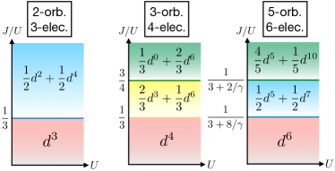
Figure 1: Atomic limit phase diagrams at $T=0$, $U>0$, and $J/U\geq 0$ for three different models ($M=2,3$, and $5$ systems) with $n_{d}=M+1$. The lowest-energy configurations are indicated at each region. The VS phase is highlighted with skyblue region.

The ground state configurations of atomic limit at vanishing temperature ($T=0$) are presented in Fig. 1. Here we use notation $cd^{n}$ to denote the ratio ($c$) of sites having $n$-electron occupation in the configuration. The homogeneous phases ($d^{n_{d}}$) occupy the small $J/U$ regions relevant to most of real materials.

For large $J/U$, on the other hand, the mixed valence phases emerge. For all the cases with Kanamori interaction ($1/\gamma=0$ for $M=5$), the transition occurs from a homogeneous to a mixed valence state when $J/U>1/3$, i.e., $U-3J<0$. Only the $M=2$ case shows VS transition ($d^{N}\rightarrow(d^{(N+1)}+d^{(N-1)})/2$) under this form of interaction. This VS phenomenon is the direct manifestation of the negative $U_{\mathrm{eff}}$: $U_{\mathrm{eff}}\equiv E_{N+1}+E_{N-1}-2E_{N}<0$ where $E_{N}$ is energy of the lowest-lying $N$-electron state Anderson (1975); Katayama-Yoshida and Zunger (1985); Varma (1988). The $1/\gamma\neq 0$ case of $M=5$ also leads to VS, albeit an extreme form of mixed valence preempts the region of $J/U>1/(3+2/\gamma)$ masking the VS phase (see the rightmost panel in Fig. 1 or see Ref. Strand (2014) for the $M=5$ case). To summarize, we identify $M=2$ case as the minimal model for $J$-driven VS phenomenon.

With insight obtained above, we now turn to the actual lattice problem with nonzero hopping. In order to focus on generic features rather than material specific ones, we consider the infinite dimensional Bethe lattice of semicircular density of states with half-bandwidth $D=1$. $D$ is hereafter used as the unit of energy. We solve the $M=2$ case with $n_{d}=3$ (particle-hole symmetric about $N=2$). The interaction form of Eq. (1) is used for non-hybridized degenerate two orbitals. The model is solved within the dynamical mean-field theory (DMFT) Georges et al. (1996) employing comctqmc implementation Choi et al. (2019) of the hybridization-expansion continuous-time quantum Monte Carlo Gull et al. (2011) as an impurity solver. Unless otherwise specified, $T=0.01$. We restrict ourselves to paramagnetic solutions without spatial symmetry-breaking.

Central physical quantity of the present study is the onset temperatures of screening of spin and orbital degrees of freedom. These two temperatures, $T^{\mathrm{onset}}_{\mathrm{spin}}$ and $T^{\mathrm{onset}}_{\mathrm{orb}}$, are defined as the temperature below which the Curie law of unscreened local spin/orbital moment starts to become violated and screening sets in Deng et al. (2019). A hallmark of strong Hundness is the separation of these two temperatures: $T^{\mathrm{onset}}_{\mathrm{orb}}\gg T^{\mathrm{onset}}_{\mathrm{spin}}$ yielding a range of temperature in which unscreened local spin moment coexists with the screened orbital degrees of freedom Okada and Yosida (1973); Yin et al. (2012); Horvat et al. (2016); Aron and Kotliar (2015); Horvat et al. (2019); Stadler et al. (2015, 2019); Deng et al. (2019). We will measure the separation of two $T^{\mathrm{onset}}$ as $\Delta T^{\mathrm{onset}}\equiv T^{\mathrm{onset}}_{\mathrm{orb}}-T^{\mathrm{onset}}_{\mathrm{spin}}$. To locate the onset temperatures, we first evaluate the local spin/orbital susceptibilities: $\chi_{\mathrm{s/o}}=\int_{0}^{1/T}{d\tau\big{(}\langle{O}_{\mathrm{s/o}}(\tau){O}_{\mathrm{s/o}}\rangle-\langle{O}_{\mathrm{s/o}}\rangle^{2}\big{)}}$, where ${O}_{\mathrm{s}}(\tau)=\sum_{m}n_{m\uparrow}(\tau)-n_{m\downarrow}(\tau)$ for spin and ${O}_{\mathrm{o}}(\tau)=\sum_{\sigma}n_{1\sigma}(\tau)-n_{2\sigma}(\tau)$ for orbital ($\tau$: imaginary time) up to $T=1$, and then fit high-$T$ data to the following formula: $\chi_{\mathrm{s/o}}\propto 1/(T+T^{\mathrm{onset}}_{\mathrm{spin/orb}})$.

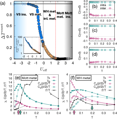
Figure 2: (a) $\Delta T^{\mathrm{onset}}$ as a function of $U_{\mathrm{eff}}$ obtained from $2\leq U/D\leq 8$ and $0\leq J/U\leq 0.5$. The red dotted line indicates the approximate value of $U_{\mathrm{eff}}$ below which $\Delta T^{\mathrm{onset}}>0$. The black dotted line denotes $U_{\mathrm{eff}}=0$. We used $T=0.05$ to stabilize the VS insulator phase com (a). The diamond symbols denote the region in which $T^{\mathrm{onset}}_{\mathrm{orb}}>1$. Inset: $T^{\mathrm{onset}}_{\mathrm{orb}}/T^{\mathrm{onset}}_{\mathrm{spin}}$ as a function of $U_{\mathrm{eff}}$. (b–d) $C_{\mathrm{intra}}$ (green square) and $C_{\mathrm{inter}}$ (magenta circle) at $U=4$ for (b) Mott metal ($J/U=0.15$; $U_{\mathrm{eff}}=2.2$), (c) WH metal ($J/U=0.3$; $U_{\mathrm{eff}}=0.4$), and (d) VS metal ($J/U=0.37$; $U_{\mathrm{eff}}=-0.44$). (e–f) $\chi_{\mathrm{s/o}}$, $\Gamma/T$, and $C_{\mathrm{s/o}}(\beta/2)/T$ plotted as a function of $T$ at $U=4$ for (e) Mott metal ($J/U=0.15$; $U_{\mathrm{eff}}=2.2$) and (f) WH metal ($J/U=0.3$; $U_{\mathrm{eff}}=0.4$). $T^{\mathrm{peak}}_{\mathrm{spin/orb}}$ are marked with magenta (spin) and green (orbital) arrows. The grey dashed lines are guide to the eye to indicate quasilinearity of $\Gamma/T$ (i.e., $\Gamma\sim T^{2}$).

Figure 2(a) presents our calculated $\Delta T^{\mathrm{onset}}$ as a function of $U_{\mathrm{eff}}$. Most interestingly, we found a generic scaling relation between $\Delta T^{\mathrm{onset}}$ and $U_{\mathrm{eff}}$. Note also that $T^{\mathrm{onset}}_{\mathrm{orb}}/T^{\mathrm{onset}}_{\mathrm{spin}}$ clearly shows the same trend as shown in the inset of Fig. 2(a). This implies that $U_{\mathrm{eff}}$ ($U_{\mathrm{eff}}=U-3J$ for our case) is the crucial factor, rather than $U$ or $J$ alone, for the separation of two onset temperatures. This result is consistent with the recent comparative study of real materials Deng et al. (2019), and demonstrates the generality holding for wide range of $U$ and $J/U$ in the two-orbital model.

By looking at Fig. 2(a), one can first notice the presence of two distinctive types of insulators, namely the Mott and valence-skipping (VS) insulators at large positive and negative values of $U_{\mathrm{eff}}$, respectively. The former is the result of suppressed charge fluctuations localizing electron motions, thereby maximizing the probability of $|N=n_{d}=3,S=1/2\rangle$ multiplets ($N$: charge, $S$: spin). By contrast, the latter form of insulator exhibits the predominance of two multiplets, $|2,1\rangle$ and $|4,0\rangle$ with largely suppressed $|3,1/2\rangle$ probability because $U_{\mathrm{eff}}<0$ sup . The presence of these two phases is reminiscent of the atomic limit result (see Fig. 1).

Interestingly, we identify distinctive regimes within metallic phase intervening between the two insulators. When $U\gg J$, a metal with $\Delta T^{\mathrm{onset}}\simeq 0$ is found to appear near a Mott insulator where Mottness dominates over Hundness (see Fig. 2(a)). To gain some understanding of this behavior, we resort to a low-energy Kondo model by performing a Schrieffer-Wolff transformation of relevant impurity Hamiltonian Schrieffer and Wolff (1966). The resulting Kondo coupling constants ($\mathcal{J}^{i}$) when $U>J$ read $\mathcal{J}^{i}_{U,J}\simeq\mathcal{J}^{i}_{U,J=0}+\mathcal{O}(\frac{J}{U^{2}})+\mathcal{O}(\frac{J^{2}}{U^{3}})+\cdots$ because $\mathcal{J}^{i}_{U,J}\sim V^{2}/{\Delta E}$. Here, $V$ is the bath-impurity hybridization strength and $\Delta E$ is the charge excitation energy from $N=n_{d}$ to $N=n_{d}\pm 1$ subspaces. In the regime of $U\gg J$, $\mathcal{J}^{i}_{U,J}\simeq\mathcal{J}^{i}_{U,J=0}$ by which the system approximates to a $\mathrm{SU(4)}$ model having $\mathcal{J}^{\mathrm{spin}}=\mathcal{J}^{\mathrm{orb}}$. In this case, the relation $\mathcal{J}^{\mathrm{spin}}=\mathcal{J}^{\mathrm{orb}}$ also holds under renormalization group flow Kuramoto (1998); Aron and Kotliar (2015), thereby the Kondo screening of spin and orbital occur simultaneously. In this respect, we identify a regime of strong Mottness ($U\gg J$) with $\Delta T^{\mathrm{onset}}\simeq 0$. Following the terminology of Ref. Deng et al. (2019); Stadler et al. (2019), we call the metallic regime of $\Delta T^{\mathrm{onset}}\simeq 0$ a Mott metal (see Fig. 2(a)).

On the contrary, there exist metals with a finite $\Delta T^{\mathrm{onset}}$. Near VS insulator where $U_{\mathrm{eff}}<0$, a correlated metal emerges exhibiting a tendency of valence-skipping, which we call a VS metal (Fig. 2(a)). In order to characterize this metal, we examine the sign of $C_{\mathrm{inter}}$ ($C_{\mathrm{intra/inter}}=\langle\delta n_{m}\delta n_{m^{\prime}}\rangle$ where $\delta n_{m}=\sum_{\sigma}n_{m\sigma}-\langle\sum_{\sigma}n_{m\sigma}\rangle$ and $m\neq m^{\prime}$ for $C_{\mathrm{inter}}$ while $m=m^{\prime}$ for $C_{\mathrm{intra}}$). As VS metal emerges when $U_{\mathrm{eff}}<0$, multiplets in $N={2}$ and $N={4}$ charge subspaces are lower in energy than those of $N={3}$. Thus, either electrons or holes try to occupy both orbitals yielding $C_{\mathrm{inter}}>0$ in contrast to the case of metals belonging to $U_{\mathrm{eff}}>0$ (compare Fig. 2(d) with (b) and (c)). Due to this negativity of $U_{\mathrm{eff}}$, VS region is highly susceptible to the formation of charge disproportionation Strand (2014); Ryee et al. (2020a) or superconductivity Micnas et al. (1990); Hoshino and Werner (2015), thereby being detectable when accompanied by such orders.

We now turn to the metallic region where $U_{\mathrm{eff}}>0$ with $\Delta T^{\mathrm{onset}}>0$ which is of our particular interest due to the potential presence of Hund’s metallicity. Although strong Hundness is argued to be manifested by $\Delta T^{\mathrm{onset}}>0$ Deng et al. (2019), the presence of Hund’s metal regime in our two-orbital model has yet to be established. The emergence of Hund’s metallicity has been attributed to the two-faced effect of $J$ dubbed “Janus effect” suppressing the quasiparticle weight $Z$ com (b) on one hand, while enhancing $U_{c}$ ($U_{c}$: the critical value of $U$ for the Mott transition) on the other hand de’ Medici et al. (2011). Thereby it reflects the stronger correlation (i.e, reduced $Z$) induced by $J$ rather than the proximity to a Mott insulator. This effect has been clearly seen in systems with $n_{d}=M\pm 1$ among $M\geq 3$ orbitals in which the atomic ground state degeneracy is lifted by $J$ de’ Medici et al. (2011); Georges et al. (2013). On the contrary, our two-orbital system with $n_{d}=M+1=3$ hosts single hole, whereby it has been a conventional wisdom that the Janus effect is absent in two-orbital models away from half-filling.

Here we argue that, albeit weak, the Janus effect can be identified even in the two-orbital case. We first note that the conventional way of capturing this effect is to plot the evolution of $Z$ as a function of $U$, and then to examine whether the suppression of $Z$ and enhancement of $U_{c}$ simultaneously occur at a fixed $U$ as $J$ is increased, i.e., examining whether $(\partial{Z}/\partial{J})_{U}<0$ and $d{U_{c}(J)}/dJ>0$. In this strategy, however, the interorbital Coulomb energy cost, $U^{\prime}=U-2J$, is not fixed as $J$ is varied. Thus, the genuine effect of tuning $J$ is partly masked by the reduced $U^{\prime}$.

To circumvent the above difficulty, we propose an alternative “gauge” of measuring the Janus effect: examining the sign of $(\partial{Z}/\partial{J})_{U_{\mathrm{avg}}}$ where $U_{\mathrm{avg}}\equiv{1}/{M^{2}}\sum_{mm^{\prime}}\mathcal{U}_{mm^{\prime}}$ ($\mathcal{U}_{mm^{\prime}}$: elements of Coulomb interaction tensor; see SM sup ). The rationale behind this proposal is that one should count not only the intra- ($m=m^{\prime}$), but also the interorbital ($m\neq m^{\prime}$) Coulomb energy cost which may vary with $J$. For the current $M=2$ case, $U_{\mathrm{avg}}=U-J$. It is worth noting that within the Slater parametrization for $M=5$, $U_{\mathrm{avg}}=F^{0}$ ($F^{0}$: the zeroth-order Slater integral which is the monopole term of Coulomb interaction). We also point out that this kind of viewpoint is implicitly embodied in some ab initio studies (e.g., Ref. Haule and Kotliar (2009); Kang and Kotliar (2020)) by the use of Slater parametrization of the Coulomb interaction with $F^{0}$ remaining unchanged while varying $J$ in searching for the Hund’s physics. With this idea in mind, we plot $Z$ vs. $U_{\mathrm{avg}}$ in Fig. 3(a). One can now clearly capture the Janus effect; namely, $(\partial{Z}/\partial{J})_{U_{\mathrm{avg}}}<0$ and $d{U_{c}}(J)/d{J}>0$. We suspect that this reduction of $Z$ by $J$ is attributed to the lifted degeneracy in $N=2$ charge subspace. In this subspace, $J$ elevates the energy of $|2,0\rangle$ states and lowers that of $|2,1\rangle$. The enhanced fluctuation between $|2,1\rangle$ and $|3,1/2\rangle$ suppresses $\mathcal{J}^{\mathrm{spin}}$ as in the case of $M\geq 3$ models with $n_{d}=M\pm 1$ Yin et al. (2011a, 2012); Horvat et al. (2016); Aron and Kotliar (2015). In the meanwhile, atomic state of $n_{d}$ subspace ($N=3$) is not affected by $J$ since it plays no role when single electron/hole is occupied. As a result, overall influence of $J$ is weaker than the $M\geq 3$ cases. In this sense, we call our metallic regime satisfying $(\partial{Z}/\partial{J})_{U_{\mathrm{avg}}}<0$ (or $(\partial{Z}/\partial{J})_{U}<0$) and $d{U_{c}}(J)/d{J}>0$ a “weak” Hund’s (WH) metal (Fig. 3(b)).

Figure 3: (a) $Z$ as a function of $U_{\mathrm{avg}}~{}(=U-J)$ for several $J/U~{}(=\frac{J/U_{\mathrm{avg}}}{1+J/U_{\mathrm{avg}}})$. (b) Phase diagram with color scheme representing $Z$. The red and black dotted lines indicate the same as in Fig. 2(a). The green dotted line is an estimated boundary of $J/U$ above which the Janus effect emerges: $(\partial{Z}/\partial{J})_{U_{\mathrm{avg}}}<0$ while $d{U_{c}}(J)/d{J}>0$. Green diamonds are actual crossing points where $(\partial{Z}/\partial{J})_{U_{\mathrm{avg}}}=0$, whereas blue ones are $(\partial{Z}/\partial{J})_{U}=0$ plotted for comparison. A set of $U$ and $J/U$ values belonging to the same $U_{\mathrm{avg}}$ are connected with a white solid line. (c) Characteristic features of different correlated metals. Here, $+/-$ denote the sign of the corresponding quantity.

As a central result of our study, we present the phase diagram exhibiting different metallic regimes; see Fig. 3(b). In Fig. 3(c), we also summarize characteristic features of these correlated metals. The green dotted line in Fig. 3(b) denotes $J/U$ above which the Janus effect exists. Hence we now further classify the region of $U_{\mathrm{eff}}>0$ and $\Delta T^{\mathrm{onset}}>0$ into two: WH metal exhibiting the Janus effect and intermediate metal which emerges in an “intermediate” region between the WH and Mott metals. In the intermediate metal, $J$ alleviates the correlation strength, i.e., $(\partial{Z}/\partial{J})_{U_{\mathrm{avg}}}>0$, although spin-orbital separation ($\Delta T^{\mathrm{onset}}>0$) occurs.

Notable feature of this phase diagram is that near $J/U=1/3$ line which is the boundary between WH and VS metals, quasiparticle survives up to an arbitrarily large $U$. Indeed, $(\partial Z/\partial U_{\mathrm{avg}})_{J/U=1/3}\rightarrow 0$ while $Z$ remains small but finite as $U_{\mathrm{avg}}$ is increased (Fig. 3(a)). This is because the lowest-energy atomic multiplets in $N=n_{d}$ and $N=n_{d}\pm 1$ subspaces are degenerate or sufficiently close in energy around this line resulting in $U_{\mathrm{eff}}=U-3J\simeq 0$. As a result, hopping processes become feasible, which otherwise should be blocked due to a large Coulomb energy cost Isidori et al. (2019).

Having established an overall picture, we now further examine the spin-orbital separation via long-time spin/orbital correlators at $\tau=\beta/2$ ($\beta=1/T$): $C_{\mathrm{s/o}}(\beta/2)=\langle{O}_{\mathrm{s/o}}(\beta/2){O}_{\mathrm{s/o}}\rangle-\langle{O}_{\mathrm{s/o}}\rangle^{2}$ in Fig. 2(e–f). At sufficiently low temperatures, $C_{\mathrm{s/o}}(\beta/2)$ scales as $C_{\mathrm{s/o}}(\beta/2)\sim\big{(}T/(\mathrm{sin}(\pi/2))\big{)}^{\alpha}$ with $\alpha=2$ in a Fermi-liquid, while $\alpha=1$ in the crossover between local moment and the Fermi-liquid Werner et al. (2008); Cha et al. (2020). In the unscreened local moment regime, $C_{\mathrm{s/o}}(\beta/2)$ is basically $T$-independent and $\chi_{\mathrm{s/o}}\simeq C_{\mathrm{s/o}}(\beta/2)/T$ (Fig. 2(e–f)). In light of this observation, we investigate $C_{\mathrm{s/o}}(\beta/2)/T$ for an extended range of $T$. These quantities should be $T$-linear in the Fermi-liquid, whereas scale as $1/T$ in the local moment regime. As a consequence, a narrow region of crossover between these two emerges forming a hump of $C_{\mathrm{s/o}}(\beta/2)/T$. Temperatures at which peaks of $C_{\mathrm{s/o}}(\beta/2)/T$ appear ($T^{\mathrm{peak}}_{\mathrm{spin/orb}}$) are marked with arrows in Fig. 2(e–f). One can clearly notice that the $T^{\mathrm{peak}}_{\mathrm{spin}}$ coincides with $T^{\mathrm{peak}}_{\mathrm{orb}}$ in the Mott metal whereas two crossover temeratures become separated in the metals with finite $\Delta T^{\mathrm{onset}}$ such as WH metal. Furthermore, below $T^{\mathrm{peak}}_{\mathrm{spin}}$ the quasiparticle scattering rate $\Gamma=-Z\mathrm{Im}[\Sigma(i\omega)]\big{|}_{\omega\rightarrow 0}$ roughly follows the Fermi-liquid behavior ($\Gamma\propto T^{2}$). This result is consistent with the observation that $C_{\mathrm{s}}(\beta/2)/T$ is sublinear in $T$ when $T<T^{\mathrm{peak}}_{\mathrm{spin}}$.

While we mainly focus on the generic features of Mott and Hund physics, its relevance to RE_1-δSr_δNiO₂ is of particular interest. Our two orbitals can be regarded as Ni-$d_{x^{2}-y2}$ and another Ni-$d$ orbital. Ab initio estimate of Coulomb interaction for a Ni-$e_{g}$ model reads $U/D\simeq 1.7$ and $J/U\simeq 0.2$ Sakakibara et al. (2020), which falls into the WH metal region (Fig. 3(b)). However, $\Delta$, the on-site energy level splitting between two orbitals, and its competition with $J$ should also be taken into account. If $\Delta$ dominates over $J$, singlet $|2,0\rangle$ would be favored over triplet $|2,1\rangle$ hampering strong Hund’s physics. In the presence of $\Delta$, eigenvalues of local Hamiltonian are $E_{|2,0\rangle}=U-\Delta-\sqrt{J^{2}+\Delta^{2}}-2\mu$ and $E_{|2,1\rangle}=U-3J-\Delta-2\mu$ for $|2,0\rangle$ and $|2,1\rangle$, respectively sup . Hence, the criterion for predominance of $|2,1\rangle$ over $|2,0\rangle$ (i.e., $E_{|2,1\rangle}<E_{|2,0\rangle}$) is $J/\Delta>\sqrt{2}/4\simeq 0.354$. However, estimated value $J/\Delta\simeq 0.3$ for Nd_0.8Sr_0.2NiO₂ between two Ni-$e_{g}$ Sakakibara et al. (2020); Lechermann (2020b) is slightly smaller than the “bare” critical value $J/\Delta\simeq 0.354$. In this respect, nickelates may belong to the competing region where large $J/U$ favors Hund’s metallicity while $J/\Delta$ which is slightly smaller than its threshold value refrains from forming high-spin in the two-hole atomic state (see SM for related DMFT results sup ). Thus, metallic nature of doped nickelates are sensitive to the small changes in $J/\Delta$. Interestingly indeed, recent full-band ab initio study reports higher weight of $|2,1\rangle$ than $|2,0\rangle$ Kang et al. (2020) indicating the effective enhancement of $J/\Delta$. Further studies are highly desirable to confirm our picture.

To conclude, we have identified distinctive correlated metal regimes emerging out of two-orbital Hubbard model at quarter-filling. This simple model is revealed to be differentiated from three- as well as five-orbital models in their Hund’s metal active fillings, showing the transition to the VS phases. We found a generic scaling relation between the degree of spin-orbital separation ($\Delta T^{\mathrm{onset}}$) and $U_{\mathrm{eff}}$, and established a weak Hund’s metal behavior in which $J$ enhances the correlation strength. We also discussed the implications of our two-orbital picture for the nature of metallic state of RE_1-δSr_δNiO₂. We also remark that in this line of multiorbital viewpoint on nickelates, the role of nonlocal correlations/interactions and the emergence of symmetry-broken phases Villar Arribi and de’ Medici (2018); de’ Medici (2017); Steiner et al. (2016); Hoshino and Werner (2015, 2016); Ryee et al. (2020a); Dumitrescu et al. (2016); Rodriguez and Melendrez (2018) are intriguing open problems. In addition to RE_1-δSr_δNiO₂, the low-energy physics of RNiO₃ (R: rare-earth elements) is reported to be well described by Ni-$e_{g}$ bands Subedi et al. (2015); Seth et al. (2017). Thus, a series of analysis presented in this study should also provide useful insights to these compounds.

Acknowledgement. S.R. and M.J.H. were supported by Creative Materials Discovery Program through NRF (2018M3D1A1058754) and Basic Science Research Program (2018R1A2B2005204). S.C. was supported by the U.S. Department of Energy, Office of Science, Basic Energy Sciences as a part of the Computational Materials Science Program. This research used resources of the National Energy Research Scientific Computing Center (NERSC), a U.S. Department of Energy Office of Science User Facility operated under Contract No. DE-AC02-05CH11231.

Supplemental material for
“Hund physics landscape of two-orbital system”

Siheon Ryee,¹ Myung Joon Han,¹ and Sangkook Choi^2
1Department of Physics, KAIST, Daejeon 34141, Republic of Korea
²Condensed Matter Physics and Materials Science Department,
Brookhaven National Laboratory, Upton, NY 11973, USA

Slater parametrization for five-orbital models

We first consider on-site Coulomb interaction tensor defined by:

$$\begin{split}&\mathcal{U}_{m_{1}m_{2}m_{3}m_{4}}\\ &\equiv\int d\mathbf{r}d\mathbf{r}^{\prime}\phi^{*}_{m_{1}}(\mathbf{r})\phi_{m_{3}}(\mathbf{r})V(\mathbf{r},\mathbf{r}^{\prime})\phi^{*}_{m_{2}}(\mathbf{r}^{\prime})\phi_{m_{4}}(\mathbf{r}^{\prime}),\end{split}$$ (1)

where $\phi_{m}(\mathbf{r})$ is a localized atomiclike basis function for orbital $m$. $V(\mathbf{r},\mathbf{r}^{\prime})$ is a Coulomb potential which is assumed to be static for the present case. One widely adopted strategy to generate tensor elements is resorting to the following formula assuming rotational symmetry:

$$\begin{split}&\mathcal{U}_{m_{1}m_{2}m_{3}m_{4}}\\ &=\sum_{\{m_{i}^{\prime}\}}\Big{[}S_{m_{1}m_{1}^{\prime}}S_{m_{2}m_{2}^{\prime}}\Big{\{}\sum_{k=0}^{2l}\alpha_{k}(m_{1}^{\prime},m_{2}^{\prime},m_{3}^{\prime},m_{4}^{\prime})F^{k}\Big{\}}\\ &\quad\times S^{-1}_{m_{3}^{\prime}m_{3}}S^{-1}_{m_{4}^{\prime}m_{4}}\Big{]}.\end{split}$$ (2)

Here $\alpha_{k}$ refers to Racah-Wigner numbers, $F^{k}$ to Slater integrals, and $l$ to angular momentum quantum number ($l=2$ for $d$-orbitals). $S$ is a transformation matrix from spherical harmonics to the predefined local basis sets. For the evaluation of $F^{k}$ in a solid environment, one requires advanced techniques, and thus it is often treated as a controllable parameter.

As a demonstration, we list below matrix elements of intra/inter-orbital Coulomb interaction $\mathcal{U}_{mm^{\prime}mm^{\prime}}$ using cubic harmonics basis. Matrix elements are presented in the following ordering: $d_{x^{2}-y^{2}},d_{z^{2}},d_{xy},d_{yz},d_{xz}$ Pavarini et al. (2011).

$$\begin{split}&\mathcal{U}_{mm^{\prime}mm^{\prime}}\equiv\mathcal{U}_{mm^{\prime}}=\\ &\begin{pmatrix}\mathcal{U}&\mathcal{U}-2J_{2}&\mathcal{U}-2J_{3}&\mathcal{U}-2J_{1}&\mathcal{U}-2J_{1}\\ \mathcal{U}-2J_{2}&\mathcal{U}&\mathcal{U}-2J_{2}&\mathcal{U}-2J_{4}&\mathcal{U}-2J_{4}\\ \mathcal{U}-2J_{3}&\mathcal{U}-2J_{2}&\mathcal{U}&\mathcal{U}-2J_{1}&\mathcal{U}-2J_{1}\\ \mathcal{U}-2J_{1}&\mathcal{U}-2J_{4}&\mathcal{U}-2J_{1}&\mathcal{U}&\mathcal{U}-2J_{1}\\ \mathcal{U}-2J_{1}&\mathcal{U}-2J_{4}&\mathcal{U}-2J_{1}&\mathcal{U}-2J_{1}&\mathcal{U}\end{pmatrix},\end{split}$$ (3)

where

$$\mathcal{U} =F^{0}+\frac{4}{49}(F^{2}+F^{4})=F^{0}+\frac{8}{5}\mathcal{J}$$ (4)

$$\mathcal{J} =\frac{5}{98}(F^{2}+F^{4})$$ (5)

$$J_{1} =\frac{3}{49}F^{2}+\frac{20}{441}F^{4}$$ (6)

$$J_{2} =-2\mathcal{J}+3J_{1}$$ (7)

$$J_{3} =6\mathcal{J}-5J_{1}$$ (8)

$$J_{4} =4\mathcal{J}-3J_{1}.$$ (9)

Matrix elements of exchange terms $\mathcal{U}_{mm^{\prime}m^{\prime}m}$ can also be evaluated from Eq. (2) in a similar manner:

$$\mathcal{U}_{mm^{\prime}m^{\prime}m}\equiv\mathcal{J}_{mm^{\prime}}=\begin{pmatrix}\mathcal{U}&J_{2}&J_{3}&J_{1}&J_{1}\\ J_{2}&\mathcal{U}&J_{2}&J_{4}&J_{4}\\ J_{3}&J_{2}&\mathcal{U}&J_{1}&J_{1}\\ J_{1}&J_{4}&J_{1}&\mathcal{U}&J_{1}\\ J_{1}&J_{4}&J_{1}&J_{1}&\mathcal{U}\end{pmatrix}.$$ (10)

Note that when $\mathcal{J}=J_{1}$, or equivalently when $F^{4}/F^{2}=1.8$, elements of Eq. (3) and Eq. (10) become $\mathcal{U}$ when $m=m^{\prime}$; $\mathcal{U}-2\mathcal{J}$ in Eq. (3) and $\mathcal{J}$ in Eq. (10) when $m\neq m^{\prime}$, which leads to the form of Eq. (1) in the main text. Hence, we can identify Kanamori parameters $U$ and $J$ as $U=\mathcal{U}=F^{0}+4(F^{2}+F^{4})/49$ and $J=\mathcal{J}=3F^{2}/49+20F^{4}/441$, respectively, for five-orbital models. For most of $d$-orbital systems, however, $F^{4}/F^{2}$ is far from this Kanamori limit of $F^{4}/F^{2}=1.8$, approximately being $F^{4}/F^{2}\simeq 0.65$ for 3$d$ systems Vaugier et al. (2012).

In the main text, we followed the strategy of Strand Strand (2014), parametrizing $F^{k}$ as follows:

$$F^{0} =U-\frac{8}{5}J$$ (11)

$$F^{2} =49\big{(}\frac{1}{\gamma}+\frac{1}{7}\big{)}J$$ (12)

$$F^{4} =\frac{63}{5}J,$$ (13)

where $1/\gamma$ controls the relative strength of anisotropy of Coulomb interaction. In this way, $1/\gamma=0$ naturally corresponds to $F^{4}/F^{2}=1.8$ which is the Kanamori limit resulting in $U=\mathcal{U}$ and $J=\mathcal{J}$. For more realistic cases of $F^{4}/F^{2}\simeq 0.65$, $1/\gamma\simeq 1/4$. We finally remark that one should not be confused with the current definition of Hubbard $U$ and Hund’s coupling $J$ with what is commonly adopted in most of literatures for five-orbital systems, which is $U=F^{0}$ and $J=(F^{2}+F^{4})/14$.

$J$ vs. $U$ phase diagram and atomic multiplet probability.

Figure S1(a) presents corresponding $J$ vs. $U$ phase diagram of Fig. (3)(b) in the main text. One can notice the presence of two correlated insulators and metals intervening between the two insulators. Note that $dU_{c}(J)/dJ>0$ is clearly seen in this plot: a small increment of $J$ always pushes $U_{c}$ to a larger value.

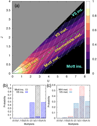
Figure S1: (a) $J$ vs. $U$ phase diagram of $Z$. (b–c) Local multiplet probability profiles of four different regimes. Each multiplet is labeled in terms of $(N,S)$. $U$ and $J/U$ corresponding to each profile are $U=5,J/U=0.1$ ($U_{\mathrm{eff}}=3.5$) for Mott insulator, $U=5,J/U=0.5$ ($U_{\mathrm{eff}}=-2.5$) for VS insulator, $U=2,J/U=0.25$ ($U_{\mathrm{eff}}=0.5$) for WH metal, and $U=2,J/U=0.45$ ($U_{\mathrm{eff}}=-0.7$) for VS metal.

In Fig. S1(b–c), we present multiplet probabilities. The Mott insulator is the result of suppressed charge fluctuations localizing electron motions. Thus $|N=3,S=1/2\rangle$ multiplet probability is maximized ($N$: charge, $S$: spin). By contrast, the VS insulator exhibits the predominance of two multiplets: $|2,1\rangle$ and $|4,0\rangle$ with largely suppressed $|3,1/2\rangle$ probability. In both WH and VS metals, the high spin $S=1$ is dominant in the $N=2$ charge subspace due to the effect of sizeable $J$ blocking the low-spin $S=0$ state. As VS metal emerges when $U_{\mathrm{eff}}<0$, multiplets in $|2,1\rangle$ and $|4,0\rangle$ are lower in energy than $|3,1/2\rangle$ exhibiting enhanced probabilitiy of $|2,1\rangle$ and $|4,0\rangle$ compared to the WH metal case.

We found that $T^{\mathrm{onset}}_{\mathrm{spin}}$ is distinctively higher in $U/D=1$ than the larger $U/D$ regions ($U/D\geq 2$) as shown in Fig. S1 exhibiting clear deviation of $U/D=1$ case from the rest. Considering that $T^{\mathrm{onset}}_{\mathrm{spin}}$ is a proxy for correlation strength, $U/D=1$ case should basically fall into the weakly correlated regime. Indeed large quasiparticle weight $Z$ is obtained near $U/D=1$ (see Fig. S1(a)).

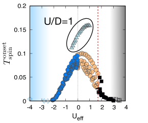
Figure S2: $T^{\mathrm{onset}}_{\mathrm{spin}}$ as a function of $U_{\mathrm{eff}}$. Filled triangles correspond to the $U/D=1$ case.

The effect other parametrizations of the local interaction I.

In searching for the Janus effect, we argued that due to the choice of $U^{\prime}=U-2J$, genuine effect of $J$ is masked by $U^{\prime}$ which not fixed when $J$ is tuned. To test this idea, we set $U^{\prime}=\alpha U$ with $\alpha$ being a tunable constant in Eq. (1) in the main text. In this way, $U^{\prime}$ as well as $U$ is disentangled from $J$, thereby more clear identification of their influences becomes feasible. As a demonstration, we present $Z$ obtained from $\alpha=0.7$ in Fig. S3. Note that in this case, $U_{\mathrm{eff}}=0.7U-J$. Thus $J/U\leq 0.7$ guarantees that $U_{\mathrm{eff}}\geq 0$. The Janus effect is observed, i.e, $(\partial{Z}/\partial{J})_{U}<0$ and $d{U_{c}}(J)/d{J}>0$, corroborating our conclusion that $J$ does induce this effect in two-orbital models.

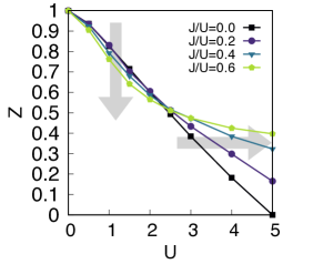
Figure S3: $Z$ as a function of $U$ with varying $J/U$. $U^{\prime}=0.7U$.

The effect other parametrizations of the local interaction II.

The generalization of the local interaction Hamiltonian in Eq. (1) in the main text reads

$$\begin{split}H_{\mathrm{loc}}&=U\sum_{m}{n_{m\uparrow}n_{m\downarrow}}+(U^{\prime}-J\delta_{\sigma\sigma^{\prime}})\sum_{m,m^{\prime},\sigma,\sigma^{\prime}}^{m<m^{\prime}}{n_{m\sigma}n_{m^{\prime}\sigma^{\prime}}}\\ &+\sum_{m,m^{\prime}}^{m\neq m^{\prime}}(J_{\mathrm{X}}d^{\dagger}_{m\uparrow}d^{\dagger}_{m^{\prime}\downarrow}d_{m\downarrow}d_{m^{\prime}\uparrow}+J_{\mathrm{P}}d^{\dagger}_{m\uparrow}d^{\dagger}_{m\downarrow}d_{m^{\prime}\downarrow}d_{m^{\prime}\uparrow}).\end{split}$$ (14)

The last two terms are now decoupled from $J$ which is responsible for the energy gain by forming the parallel spins (i.e., Hund’s first rule). Throughout the manuscript, we have considered the common choice of setting $U^{\prime}=U-2J$ and $J=J_{\mathrm{X}}=J_{\mathrm{P}}$. To check the robustness of the existence of various metallic regimes discussed in the main text with respect to the choice of parametrization, we now consider a different setting: $U^{\prime}=U-2J$ and $J/2=J_{\mathrm{X}}=J_{\mathrm{P}}$. In this case, both orbital and spin rotational symmetries are broken. In any case, we obtained qualitatively the same phase diagram (see Fig. S4): as $J$ is increased from $J=0$, system evolves from Mott to VS insulator with four different intervening metallic regimes. Transition from WH to VS metal is found also at $U_{\mathrm{eff}}=U-3J=0$, i.e., $J\simeq 1.67$ when $U=5$ as presented in Fig. S4(a).

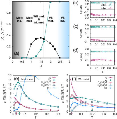
Figure S4: (a) $Z$ (black squares) and $\Delta T^{\mathrm{onset}}$ (green circles and diamonds) as a function of $J$ at $U=5$ using local interaction form of Eq. (14) with $U^{\prime}=U-2J$ and $J/2=J_{\mathrm{X}}=J_{\mathrm{P}}$. The diamond symbol denotes the region in which $T^{\mathrm{onset}}_{\mathrm{orb}}>1$. (b–d) $C_{\mathrm{intra}}$ (green squares) and $C_{\mathrm{inter}}$ (magenta circles) at $U=5$ for (b) Mott metal ($J/U=0.2$; $U_{\mathrm{eff}}=2$), (c) WH metal ($J/U=0.3$; $U_{\mathrm{eff}}=0.5$), and (d) VS metal ($J/U=0.4$; $U_{\mathrm{eff}}=-1$). (e–f) $\chi_{\mathrm{s/o}}$, $\Gamma/T$, and $C_{\mathrm{s/o}}(\beta/2)/T$ plotted as a function of $T$ at $U=5$ for (e) Mott metal ($J/U=0.2$; $U_{\mathrm{eff}}=2$) and (f) WH metal ($J/U=0.3$; $U_{\mathrm{eff}}=0.5$). $T^{\mathrm{peak}}_{\mathrm{spin/orb}}$ are marked with magenta (spin) and green (orbital) arrows. The grey dashed lines are guide to the eye to indicate quasilinearity of $\Gamma/T$ (i.e., $\Gamma\sim T^{2}$).

	Eigenstates	$N$	$S$	$S_{z}$	Eigenvalues
$|1\rangle$	$|0,0\rangle$	0	0	0	0
$|2\rangle$	$|0,\uparrow\rangle$	1	1/2	1/2	$-\Delta-\mu$
$|3\rangle$	$|0,\downarrow\rangle$	1	1/2	-1/2	$-\Delta-\mu$
$|4\rangle$	$|\uparrow,0\rangle$	1	1/2	1/2	$-\mu$
$|5\rangle$	$|\downarrow,0\rangle$	1	1/2	-1/2	$-\mu$
$|6\rangle$	$|\uparrow,\uparrow\rangle$	2	1	1	$U-3J-\Delta-2\mu$
$|7\rangle$	$\big{(}|\uparrow,\downarrow\rangle+|\downarrow,\uparrow\rangle\big{)}/\sqrt{2}$	2	1	0	$U-3J-\Delta-2\mu$
$|8\rangle$	$|\downarrow,\downarrow\rangle$	2	1	-1	$U-3J-\Delta-2\mu$
$|9\rangle$	$\big{(}|\uparrow,\downarrow\rangle-|\downarrow,\uparrow\rangle\big{)}/\sqrt{2}$	2	0	0	$U-J-\Delta-2\mu$
$|10\rangle$	$\frac{\alpha+\beta}{\sqrt{(\alpha+\beta)^{2}+J^{2}}}|\uparrow\downarrow,0\rangle-\frac{J}{\sqrt{(\alpha+\beta)^{2}+J^{2}}}|0,\downarrow\uparrow\rangle$	2	0	0	$U-\Delta-\sqrt{J^{2}+\Delta^{2}}-2\mu$
$|11\rangle$	$\frac{\alpha-\beta}{\sqrt{(\alpha-\beta)^{2}+J^{2}}}|\uparrow\downarrow,0\rangle-\frac{J}{\sqrt{(\alpha-\beta)^{2}+J^{2}}}|0,\downarrow\uparrow\rangle$	2	0	0	$U-\Delta+\sqrt{J^{2}+\Delta^{2}}-2\mu$
$|12\rangle$	$|\uparrow,\uparrow\downarrow\rangle$	3	1/2	1/2	$3U-5J-2\Delta-3\mu$
$|13\rangle$	$|\downarrow,\uparrow\downarrow\rangle$	3	1/2	-1/2	$3U-5J-2\Delta-3\mu$
$|14\rangle$	$|\uparrow\downarrow,\uparrow\rangle$	3	1/2	1/2	$3U-5J-\Delta-3\mu$
$|15\rangle$	$|\uparrow\downarrow,\downarrow\rangle$	3	1/2	-1/2	$3U-5J-\Delta-3\mu$
$|16\rangle$	$|\uparrow\downarrow,\uparrow\downarrow\rangle$	4	0	0	$6U-10J-2\Delta-4\mu$

Table S1: $\alpha=-\Delta$ and $\beta=\sqrt{J^{2}+\Delta^{2}}$. $U^{\prime}=U-2J$, $\epsilon_{1}=0$, and $\epsilon_{2}=-\Delta$ in Eq. (15). The first entry in a ket of an eigenstate is the state of orbital-1 while the second is of orbital-2.

The effect of on-site energy level splitting and implications for RE_1-δSr_δNiO₂

We now consider the following local Hamiltonian for two orbitals:

$$\begin{split}H_{\mathrm{loc}}&=U\sum_{m}{n_{m\uparrow}n_{m\downarrow}}+\sum_{mm^{\prime},\sigma\sigma^{\prime}}^{m<m^{\prime}}(U^{\prime}-J\delta_{\sigma\sigma^{\prime}}){n_{m\sigma}n_{m^{\prime}\sigma^{\prime}}}\\ &+J\sum_{m,m^{\prime}}^{m\neq m^{\prime}}(d^{\dagger}_{m\uparrow}d^{\dagger}_{m^{\prime}\downarrow}d_{m\downarrow}d_{m^{\prime}\uparrow}+d^{\dagger}_{m\uparrow}d^{\dagger}_{m\downarrow}d_{m^{\prime}\downarrow}d_{m^{\prime}\uparrow})\\ &+\sum_{m,\sigma}(\epsilon_{m}-\mu)n_{m\sigma},\end{split}$$ (15)

where $\epsilon_{m}$ is the on-site energy level of orbital $m$ ($m=1,2$). $U^{\prime}=U-2J$. Eigenvalues and corresponding eigenstates of Eq. (15) with a finite energy level splitting between two orbitals ($\epsilon_{1}=0$ and $\epsilon_{2}=-\Delta$) are presented in Table S1. Note that the lowest-energy spin state in $N=2$ subspace is determined by the ratio $J/\Delta$; eigenvalues of local Hamiltonian are $E_{S=1}=U-\Delta-\sqrt{J^{2}+\Delta^{2}}-2\mu$ for singlet $|10\rangle$ and $E_{S=0}=U-3J-\Delta-2\mu$ for triplet $|6\rangle$, $|7\rangle$, and $|8\rangle$. Hence, the criterion for predominance of triplet (i.e., $E_{S=1}<E_{S=0}$) is $J/\Delta>\sqrt{2}/4\simeq 0.354$.

With this insight, we further contemplate the effect of a finite $\Delta$ and the resulting spin state in the $N=2$ charge subspace (or equivalently, the two hole subspace) in connection with infinite-layer nickelates RE_1-δSr_δNiO₂. We take $U/D\simeq 2$ and $J/U=0.2$ relevant for a Ni-$e_{g}$ model of Nd_0.8Sr_0.2NiO₂ Sakakibara et al. (2020). Figure S5(a–b) present the hole doping ($\delta_{\mathrm{hole}}$) dependence of $Z$ of orbital-1 and the atomic multiplet probabilities of triplet $S=1$ and singlet $S=0$ states in the $N=2$ charge subspace with varying $\Delta$ obtained from our DMFT calculations.

One can notice from Fig. S5(b) that being consistent with atomic multiplet analysis, $S=1$ starts to prevail over $S=0$ when $J/\Delta>0.354$ as $\delta_{\mathrm{hole}}$ increases. However, singlet $S=0$ is predominant at the relevant value of $J/\Delta\simeq 0.3$ for Nd_0.8Sr_0.2NiO₂.

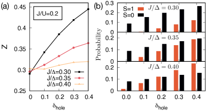
Figure S5: $\delta_{\mathrm{hole}}$ dependence of (a) $Z$ of orbital-1 at $U/D=2$ and $J/U=0.2$ with varying $\Delta$ and (b) corresponding atomic multiplet probabilities of $S=1$ (orange) and $S=0$ (black) states in the $N=2$ charge subspace.

In any case, we found that $Z$ is enhanced as $\delta_{\mathrm{hole}}$ is introduced Fig. S5(a), albeit this enhancement is gradually diminished as $J/\Delta$ is increased. Interestingly, $\delta_{\mathrm{hole}}$ dependence of $Z$ obtained from our two-orbital model (Fig. S5(a)) is consistent with several previous ab initio results reporting the enhancement of $Z$ of Ni-$d_{x^{2}-y^{2}}$ state upon hole doping Kitatani et al. (2020); Wang et al. (2020); Petocchi et al. (2020); Kang et al. (2020). Thus, it may be interpreted as a signature showing that the singlet rather than triplet dominates the two-hole subspace of RE_1-δSr_δNiO₂. This supports Mott’s metallic behavior, in line with an interpretation of recent x-ray absoption spectroscopy (XAS) data Rossi et al. (2020).

However, there is another way to explain the hole-doping induced $Z$ enhancement: $\delta_{\mathrm{hole}}$-induced $\Delta$ enhancement. Within ab initio linearized quasiparticle self-consistent GW + DMFT (LQSGW+DMFT) Kang et al. (2020), $\Delta$ is enhanced by 20 $\%$ upon 0.2 hole doping. Also interestingly, ab initio LQSGW+DMFT approach reports approximately two times larger probability of $S=1$ than that of $S=0$ in Ni-$e_{g}$ subspace Kang et al. (2020). These results suggest that extrinsic doping changes model Hamiltonian parameters. Besides, it has been reported that the majority of the doped hole goes into other orbitals than Ni-$d$ Kang et al. (2020). At $n_{d}=2.6$ ($\delta_{\mathrm{hole}}=0.4$) which corresponds the Ni-$e_{g}$ occupation of RE_0.8Sr_0.2NiO₂ obtained from ab initio LQSGW+DMFT, $Z$ increases as $\Delta$ increases as shown in Fig. S5(a). The Hund’s metal picture, which is not compatible with the aforementioned doping dependence under fixed parameters, may be reconciled with the doping-induced $Z$ enhancement in this way.

References

- Georges et al. (2013) A. Georges, L. de Medici, and J. Mravlje, Annu. Rev. Condens. Matter Phys. 4, 137 (2013).
- Haule and Kotliar (2009) K. Haule and G. Kotliar, New Journal of Physics 11, 025021 (2009), URL https://doi.org/10.1088%2F1367-2630%2F11%2F2%2F025021.
- Yin et al. (2011a) Z. Yin, K. Haule, and G. Kotliar, Nature Materials 10, 932 (2011a).
- de’ Medici et al. (2011) L. de’ Medici, J. Mravlje, and A. Georges, Phys. Rev. Lett. 107, 256401 (2011), URL https://link.aps.org/doi/10.1103/PhysRevLett.107.256401.
- Werner et al. (2008) P. Werner, E. Gull, M. Troyer, and A. J. Millis, Phys. Rev. Lett. 101, 166405 (2008), URL https://link.aps.org/doi/10.1103/PhysRevLett.101.166405.
- Hoshino and Werner (2015) S. Hoshino and P. Werner, Phys. Rev. Lett. 115, 247001 (2015), URL https://link.aps.org/doi/10.1103/PhysRevLett.115.247001.
- Stadler et al. (2015) K. M. Stadler, Z. P. Yin, J. von Delft, G. Kotliar, and A. Weichselbaum, Phys. Rev. Lett. 115, 136401 (2015), URL https://link.aps.org/doi/10.1103/PhysRevLett.115.136401.
- Yin et al. (2012) Z. P. Yin, K. Haule, and G. Kotliar, Phys. Rev. B 86, 195141 (2012), URL https://link.aps.org/doi/10.1103/PhysRevB.86.195141.
- Horvat et al. (2016) A. Horvat, R. Žitko, and J. Mravlje, Phys. Rev. B 94, 165140 (2016), URL https://link.aps.org/doi/10.1103/PhysRevB.94.165140.
- Aron and Kotliar (2015) C. Aron and G. Kotliar, Phys. Rev. B 91, 041110 (2015), URL https://link.aps.org/doi/10.1103/PhysRevB.91.041110.
- Horvat et al. (2019) A. Horvat, R. Zitko, and J. Mravlje, arXiv preprint arXiv:1907.07100 (2019).
- Deng et al. (2019) X. Deng, K. M. Stadler, K. Haule, A. Weichselbaum, J. von Delft, and G. Kotliar, Nature Communications 10, 2721 (2019).
- Stadler et al. (2019) K. Stadler, G. Kotliar, A. Weichselbaum, and J. von Delft, Annals of Physics 405, 365 (2019), ISSN 0003-4916, URL http://www.sciencedirect.com/science/article/pii/S0003491618302793.
- Isidori et al. (2019) A. Isidori, M. Berović, L. Fanfarillo, L. de’ Medici, M. Fabrizio, and M. Capone, Phys. Rev. Lett. 122, 186401 (2019), URL https://link.aps.org/doi/10.1103/PhysRevLett.122.186401.
- Ryee et al. (2020a) S. Ryee, P. Sémon, M. J. Han, and S. Choi, npj Quantum Materials 5, 19 (2020a), URL https://doi.org/10.1038/s41535-020-0221-9.
- de’ Medici et al. (2009) L. de’ Medici, S. R. Hassan, M. Capone, and X. Dai, Phys. Rev. Lett. 102, 126401 (2009), URL https://link.aps.org/doi/10.1103/PhysRevLett.102.126401.
- de’ Medici (2011) L. de’ Medici, Phys. Rev. B 83, 205112 (2011), URL https://link.aps.org/doi/10.1103/PhysRevB.83.205112.
- Bascones et al. (2012) E. Bascones, B. Valenzuela, and M. J. Calderón, Phys. Rev. B 86, 174508 (2012), URL https://link.aps.org/doi/10.1103/PhysRevB.86.174508.
- Lanatà et al. (2013) N. Lanatà, H. U. R. Strand, G. Giovannetti, B. Hellsing, L. de’ Medici, and M. Capone, Phys. Rev. B 87, 045122 (2013), URL https://link.aps.org/doi/10.1103/PhysRevB.87.045122.
- de’ Medici et al. (2014) L. de’ Medici, G. Giovannetti, and M. Capone, Phys. Rev. Lett. 112, 177001 (2014), URL https://link.aps.org/doi/10.1103/PhysRevLett.112.177001.
- Kostin et al. (2018) A. Kostin, P. O. Sprau, A. Kreisel, Y. X. Chong, A. E. Böhmer, P. C. Canfield, P. J. Hirschfeld, B. M. Andersen, and J. S. Davis, Nature Materias 17, 869 (2018).
- Kugler et al. (2019) F. B. Kugler, S.-S. B. Lee, A. Weichselbaum, G. Kotliar, and J. von Delft, Phys. Rev. B 100, 115159 (2019), URL https://link.aps.org/doi/10.1103/PhysRevB.100.115159.
- Lee et al. (2018) T.-H. Lee, A. Chubukov, H. Miao, and G. Kotliar, Phys. Rev. Lett. 121, 187003 (2018), URL https://link.aps.org/doi/10.1103/PhysRevLett.121.187003.
- Hansmann et al. (2010) P. Hansmann, R. Arita, A. Toschi, S. Sakai, G. Sangiovanni, and K. Held, Phys. Rev. Lett. 104, 197002 (2010), URL https://link.aps.org/doi/10.1103/PhysRevLett.104.197002.
- Yin et al. (2011b) Z. Yin, K. Haule, and G. Kotliar, Nature Physics 7, 294 (2011b).
- Fanfarillo et al. (2017) L. Fanfarillo, G. Giovannetti, M. Capone, and E. Bascones, Phys. Rev. B 95, 144511 (2017), URL https://link.aps.org/doi/10.1103/PhysRevB.95.144511.
- de’ Medici (2017) L. de’ Medici, Phys. Rev. Lett. 118, 167003 (2017), URL https://link.aps.org/doi/10.1103/PhysRevLett.118.167003.
- Villar Arribi and de’ Medici (2018) P. Villar Arribi and L. de’ Medici, Phys. Rev. Lett. 121, 197001 (2018), URL https://link.aps.org/doi/10.1103/PhysRevLett.121.197001.
- Belozerov et al. (2018) A. S. Belozerov, A. A. Katanin, and V. I. Anisimov, Phys. Rev. B 97, 115141 (2018), URL https://link.aps.org/doi/10.1103/PhysRevB.97.115141.
- Mravlje et al. (2011) J. Mravlje, M. Aichhorn, T. Miyake, K. Haule, G. Kotliar, and A. Georges, Phys. Rev. Lett. 106, 096401 (2011), URL https://link.aps.org/doi/10.1103/PhysRevLett.106.096401.
- Mravlje and Georges (2016) J. Mravlje and A. Georges, Phys. Rev. Lett. 117, 036401 (2016), URL https://link.aps.org/doi/10.1103/PhysRevLett.117.036401.
- Kugler et al. (2020) F. B. Kugler, M. Zingl, H. U. R. Strand, S.-S. B. Lee, J. von Delft, and A. Georges, Phys. Rev. Lett. 124, 016401 (2020), URL https://link.aps.org/doi/10.1103/PhysRevLett.124.016401.
- Lee et al. (2020) H. J. Lee, C. H. Kim, and A. Go, Phys. Rev. B 102, 195115 (2020), URL https://link.aps.org/doi/10.1103/PhysRevB.102.195115.
- Stadler (2019) K. M. Stadler, Ph.D. thesis (2019).
- Li et al. (2019) D. Li, K. Lee, B. Y. Wang, M. Osada, S. Crossley, H. R. Lee, Y. Cui, Y. Hikita, and H. Y. Hwang, Nature 572, 624 (2019).
- Osada et al. (2020) M. Osada, B. Y. Wang, B. H. Goodge, K. Lee, H. Yoon, K. Sakuma, D. Li, M. Miura, L. F. Kourkoutis, and H. Y. Hwang, Nano Letters 20, 5735 (2020), pMID: 32574061, eprint https://doi.org/10.1021/acs.nanolett.0c01392, URL https://doi.org/10.1021/acs.nanolett.0c01392.
- Lee and Pickett (2004) K.-W. Lee and W. E. Pickett, Phys. Rev. B 70, 165109 (2004), URL https://link.aps.org/doi/10.1103/PhysRevB.70.165109.
- Botana and Norman (2020) A. S. Botana and M. R. Norman, Phys. Rev. X 10, 011024 (2020), URL https://link.aps.org/doi/10.1103/PhysRevX.10.011024.
- Nomura et al. (2019) Y. Nomura, M. Hirayama, T. Tadano, Y. Yoshimoto, K. Nakamura, and R. Arita, Phys. Rev. B 100, 205138 (2019), URL https://link.aps.org/doi/10.1103/PhysRevB.100.205138.
- Sakakibara et al. (2020) H. Sakakibara, H. Usui, K. Suzuki, T. Kotani, H. Aoki, and K. Kuroki, Phys. Rev. Lett. 125, 077003 (2020), URL https://link.aps.org/doi/10.1103/PhysRevLett.125.077003.
- Jiang et al. (2020) M. Jiang, M. Berciu, and G. A. Sawatzky, Phys. Rev. Lett. 124, 207004 (2020), URL https://link.aps.org/doi/10.1103/PhysRevLett.124.207004.
- Wu et al. (2020a) X. Wu, D. Di Sante, T. Schwemmer, W. Hanke, H. Y. Hwang, S. Raghu, and R. Thomale, Phys. Rev. B 101, 060504 (2020a), URL https://link.aps.org/doi/10.1103/PhysRevB.101.060504.
- Hepting et al. (2020) M. Hepting, D. Li, C. Jia, H. Lu, E. Paris, Y. Tseng, X. Feng, M. Osada, E. Been, Y. Hikita, et al., Nature materials 19, 381 (2020).
- Goodge et al. (2020) B. H. Goodge, D. Li, M. Osada, B. Y. Wang, K. Lee, G. A. Sawatzky, H. Y. Hwang, and L. F. Kourkoutis, arXiv preprint arXiv:2005.02847 (2020).
- Ryee et al. (2020b) S. Ryee, H. Yoon, T. J. Kim, M. Y. Jeong, and M. J. Han, Phys. Rev. B 101, 064513 (2020b), URL https://link.aps.org/doi/10.1103/PhysRevB.101.064513.
- Jiang et al. (2019) P. Jiang, L. Si, Z. Liao, and Z. Zhong, Phys. Rev. B 100, 201106 (2019), URL https://link.aps.org/doi/10.1103/PhysRevB.100.201106.
- Si et al. (2020) L. Si, W. Xiao, J. Kaufmann, J. M. Tomczak, Y. Lu, Z. Zhong, and K. Held, Phys. Rev. Lett. 124, 166402 (2020), URL https://link.aps.org/doi/10.1103/PhysRevLett.124.166402.
- Werner and Hoshino (2020) P. Werner and S. Hoshino, Phys. Rev. B 101, 041104 (2020), URL https://link.aps.org/doi/10.1103/PhysRevB.101.041104.
- Hu and Wu (2019) L.-H. Hu and C. Wu, Phys. Rev. Research 1, 032046 (2019), URL https://link.aps.org/doi/10.1103/PhysRevResearch.1.032046.
- Zhang and Vishwanath (2020) Y.-H. Zhang and A. Vishwanath, Phys. Rev. Research 2, 023112 (2020), URL https://link.aps.org/doi/10.1103/PhysRevResearch.2.023112.
- Adhikary et al. (2020) P. Adhikary, S. Bandyopadhyay, T. Das, I. Dasgupta, and T. Saha-Dasgupta, Phys. Rev. B 102, 100501 (2020), URL https://link.aps.org/doi/10.1103/PhysRevB.102.100501.
- Zhang et al. (2020a) G.-M. Zhang, Y.-f. Yang, and F.-C. Zhang, Phys. Rev. B 101, 020501 (2020a), URL https://link.aps.org/doi/10.1103/PhysRevB.101.020501.
- Gao et al. (2020) J. Gao, S. Peng, Z. Wang, C. Fang, and H. Weng, National Science Review (2020), ISSN 2095-5138, nwaa218, eprint https://academic.oup.com/nsr/advance-article-pdf/doi/10.1093/nsr/nwaa218/33707658/nwaa218.pdf, URL https://doi.org/10.1093/nsr/nwaa218.
- Bernardini et al. (2020) F. Bernardini, V. Olevano, and A. Cano, Phys. Rev. Research 2, 013219 (2020), URL https://link.aps.org/doi/10.1103/PhysRevResearch.2.013219.
- Choi et al. (2020) M.-Y. Choi, K.-W. Lee, and W. E. Pickett, Phys. Rev. B 101, 020503 (2020), URL https://link.aps.org/doi/10.1103/PhysRevB.101.020503.
- Karp et al. (2020) J. Karp, A. S. Botana, M. R. Norman, H. Park, M. Zingl, and A. Millis, Phys. Rev. X 10, 021061 (2020), URL https://link.aps.org/doi/10.1103/PhysRevX.10.021061.
- Lechermann (2020a) F. Lechermann, Phys. Rev. B 101, 081110 (2020a), URL https://link.aps.org/doi/10.1103/PhysRevB.101.081110.
- Olevano et al. (2020) V. Olevano, F. Bernardini, X. Blase, and A. Cano, Phys. Rev. B 101, 161102 (2020), URL https://link.aps.org/doi/10.1103/PhysRevB.101.161102.
- Kitatani et al. (2020) M. Kitatani, L. Si, O. Janson, R. Arita, Z. Zhong, and K. Held, npj Quantum Materials 5, 59 (2020), URL https://doi.org/10.1038/s41535-020-00260-y.
- Zhang et al. (2020b) Y. Zhang, L.-F. Lin, W. Hu, A. Moreo, S. Dong, and E. Dagotto, Phys. Rev. B 102, 195117 (2020b), URL https://link.aps.org/doi/10.1103/PhysRevB.102.195117.
- Gu et al. (2020) Q. Gu, Y. Li, S. Wan, H. Li, W. Guo, H. Yang, Q. Li, X. Zhu, X. Pan, Y. Nie, et al., Nature Communications 11, 1 (2020).
- Wu et al. (2020b) X. Wu, K. Jiang, D. Di Sante, W. Hanke, J. Hu, and R. Thomale, arXiv preprint arXiv:2008.06009 (2020b).
- Zhang et al. (2020c) H. Zhang, L. Jin, S. Wang, B. Xi, X. Shi, F. Ye, and J.-W. Mei, Phys. Rev. Research 2, 013214 (2020c), URL https://link.aps.org/doi/10.1103/PhysRevResearch.2.013214.
- Petocchi et al. (2020) F. Petocchi, V. Christiansson, F. Nilsson, F. Aryasetiawan, and P. Werner, Phys. Rev. X 10, 041047 (2020), URL https://link.aps.org/doi/10.1103/PhysRevX.10.041047.
- Lechermann (2020b) F. Lechermann, Phys. Rev. X 10, 041002 (2020b), URL https://link.aps.org/doi/10.1103/PhysRevX.10.041002.
- Wang et al. (2020) Y. Wang, C.-J. Kang, H. Miao, and G. Kotliar, Phys. Rev. B 102, 161118 (2020), URL https://link.aps.org/doi/10.1103/PhysRevB.102.161118.
- Kang and Kotliar (2020) C.-J. Kang and G. Kotliar, arXiv preprint arXiv:2007.15383 (2020).
- Kang et al. (2020) B. Kang, C. Melnick, P. Semon, G. Kotliar, and S. Choi, arXiv preprint arXiv:2007.14610 (2020).
- Wan et al. (2020) X. Wan, V. Ivanov, G. Resta, I. Leonov, and S. Y. Savrasov, arXiv preprint arXiv:2008.07465 (2020).
- Rossi et al. (2020) M. Rossi, H. Lu, A. Nag, D. Li, M. Osada, K. Lee, B. Wang, S. Agrestini, M. Garcia-Fernandez, Y.-D. Chuang, et al., arXiv preprint arXiv:2011.00595 (2020).
- Li et al. (2020) D. Li, B. Y. Wang, K. Lee, S. P. Harvey, M. Osada, B. H. Goodge, L. F. Kourkoutis, and H. Y. Hwang, Phys. Rev. Lett. 125, 027001 (2020), URL https://link.aps.org/doi/10.1103/PhysRevLett.125.027001.
- Zeng et al. (2020) S. Zeng, C. S. Tang, X. Yin, C. Li, M. Li, Z. Huang, J. Hu, W. Liu, G. J. Omar, H. Jani, et al., Phys. Rev. Lett. 125, 147003 (2020), URL https://link.aps.org/doi/10.1103/PhysRevLett.125.147003.
- Strand (2014) H. U. R. Strand, Phys. Rev. B 90, 155108 (2014), URL https://link.aps.org/doi/10.1103/PhysRevB.90.155108.
- (74) See Supplemental Material for additional data and discussion.
- Anderson (1975) P. W. Anderson, Phys. Rev. Lett. 34, 953 (1975), URL https://link.aps.org/doi/10.1103/PhysRevLett.34.953.
- Katayama-Yoshida and Zunger (1985) H. Katayama-Yoshida and A. Zunger, Phys. Rev. Lett. 55, 1618 (1985), URL https://link.aps.org/doi/10.1103/PhysRevLett.55.1618.
- Varma (1988) C. M. Varma, Phys. Rev. Lett. 61, 2713 (1988), URL https://link.aps.org/doi/10.1103/PhysRevLett.61.2713.
- Georges et al. (1996) A. Georges, G. Kotliar, W. Krauth, and M. J. Rozenberg, Rev. Mod. Phys. 68, 13 (1996), URL https://link.aps.org/doi/10.1103/RevModPhys.68.13.
- Choi et al. (2019) S. Choi, P. Semon, B. Kang, A. Kutepov, and G. Kotliar, Computer Physics Communications 244, 277 (2019).
- Gull et al. (2011) E. Gull, A. J. Millis, A. I. Lichtenstein, A. N. Rubtsov, M. Troyer, and P. Werner, Rev. Mod. Phys. 83, 349 (2011), URL https://link.aps.org/doi/10.1103/RevModPhys.83.349.
- Okada and Yosida (1973) I. Okada and K. Yosida, Progress of Theoretical Physics 49, 1483 (1973), ISSN 0033-068X, URL https://doi.org/10.1143/PTP.49.1483.
- com (a) For the region of VS insulators, we found strong oscilations between and solutions at lower temperatures during DMFT iterations, and thus stable convergence was not achieved. However, whole discussion of the present paper is not affected by this limitation.
- Schrieffer and Wolff (1966) J. R. Schrieffer and P. A. Wolff, Phys. Rev. 149, 491 (1966), URL https://link.aps.org/doi/10.1103/PhysRev.149.491.
- Kuramoto (1998) Y. Kuramoto, Eur. Phys. J. B 5, 457 (1998), URL https://doi.org/10.1007/s100510050466.
- Micnas et al. (1990) R. Micnas, J. Ranninger, and S. Robaszkiewicz, Rev. Mod. Phys. 62, 113 (1990), URL https://link.aps.org/doi/10.1103/RevModPhys.62.113.
- com (b) , where is the fermionic self-energy on the Matsubara frequency axis. To evaluate , we fitted the fourth order polynomial to the lowest six Matsubara frequency following the strategy of Ref. Mravlje et al. (2011).
- Cha et al. (2020) P. Cha, N. Wentzell, O. Parcollet, A. Georges, and E.-A. Kim, Proceedings of the National Academy of Sciences 117, 18341 (2020), ISSN 0027-8424, URL https://www.pnas.org/content/117/31/18341.
- Steiner et al. (2016) K. Steiner, S. Hoshino, Y. Nomura, and P. Werner, Phys. Rev. B 94, 075107 (2016), URL https://link.aps.org/doi/10.1103/PhysRevB.94.075107.
- Hoshino and Werner (2016) S. Hoshino and P. Werner, Phys. Rev. B 93, 155161 (2016), URL https://link.aps.org/doi/10.1103/PhysRevB.93.155161.
- Dumitrescu et al. (2016) P. T. Dumitrescu, M. Serbyn, R. T. Scalettar, and A. Vishwanath, Phys. Rev. B 94, 155127 (2016), URL https://link.aps.org/doi/10.1103/PhysRevB.94.155127.
- Rodriguez and Melendrez (2018) J. P. Rodriguez and R. Melendrez, Journal of Physics Communications 2, 105011 (2018), URL https://doi.org/10.1088%2F2399-6528%2Faae0dc.
- Subedi et al. (2015) A. Subedi, O. E. Peil, and A. Georges, Phys. Rev. B 91, 075128 (2015), URL https://link.aps.org/doi/10.1103/PhysRevB.91.075128.
- Seth et al. (2017) P. Seth, O. E. Peil, L. Pourovskii, M. Betzinger, C. Friedrich, O. Parcollet, S. Biermann, F. Aryasetiawan, and A. Georges, Phys. Rev. B 96, 205139 (2017), URL https://link.aps.org/doi/10.1103/PhysRevB.96.205139.
- Pavarini et al. (2011) E. Pavarini, E. Koch, D. Vollhardt, and A. Lichtenstein, The LDA+DMFT approach to strongly correlated materials, Reihe Modeling and Simulation, Vol. 1 (2011).
- Vaugier et al. (2012) L. Vaugier, H. Jiang, and S. Biermann, Phys. Rev. B 86, 165105 (2012), URL https://link.aps.org/doi/10.1103/PhysRevB.86.165105.