Loop coproduct in Morse and Floer homology
Abstract.
By a well-known theorem of Viterbo, the symplectic homology of the cotangent bundle of a closed manifold is isomorphic to the homology of its loop space. In this paper we extend the scope of this isomorphism in several directions. First, we give a direct definition of Rabinowitz loop homology in terms of Morse theory on the loop space and prove that its product agrees with the pair-of-pants product on Rabinowitz Floer homology. The proof uses compactified moduli spaces of punctured annuli. Second, we prove that, when restricted to positive Floer homology, resp. loop space homology relative to the constant loops, the Viterbo isomorphism intertwines various constructions of secondary pair-of-pants coproducts with the loop homology coproduct. Third, we introduce reduced loop homology, which is a common domain of definition for a canonical reduction of the loop product and for extensions of the loop homology coproduct which together define the structure of a commutative cocommutative unital infinitesimal anti-symmetric bialgebra. Along the way, we show that the Abbondandolo-Schwarz quasi-isomorphism going from the Floer complex of quadratic Hamiltonians to the Morse complex of the energy functional can be turned into a filtered chain isomorphism by using linear Hamiltonians and the square root of the energy functional.
To Claude Viterbo on the occasion of his 60th birthday, with admiration
1. Introduction
For a closed manifold there are canonical isomorphisms
| (1) |
Here we use coefficients in any commutative ring , twisted in the first group by a suitable local system which restricts to the orientation local system on the space of constant loops (see Appendix A). The groups in the above chain of isomorphisms are as follows: denotes the homology of the free loop space relative to ; the positive action part of the Floer homology of a fibrewise quadratic Hamiltonian on the cotangent bundle; the positive symplectic homology of the unit cotangent bundle ; and the negative symplectic cohomology of the trivial Liouville cobordism over the unit cotangent bundle . The first isomorphism is the result of work of many people starting with Viterbo (see [39, 1, 5, 3, 35, 34, 17, 30, 7]); the second one is obvious; and the third one is a restriction of the Poincaré duality isomorphism from [19].
Restricting to field coefficients, all the groups in (1) carry natural coproducts of degree :
- •
-
•
the (secondary) pair-or-pants coproduct on defined by Abbondandolo and Schwarz [4];
-
•
the varying weights coproduct on first described by Seidel and further explored in [26];
-
•
the continuation coproduct on described in [20];
-
•
the Poincaré duality coproduct on dual to the pair-of-pants product on , described in [16].
The first result of this paper is
Theorem 1.1.
With field coefficients, all the above coproducts are equivalent under the isomorphisms in (1).
Remark 1.2 (Coproducts and field coefficients).
There is a formal algebraic reason why we need to restrict to field coefficients when speaking about homology coproducts. Given a chain complex and a chain map , we obtain a map . However, the latter factors through only if the Künneth isomorphism holds, which is the case with field coefficients. All our coproducts are defined at chain level with arbitrary coefficients, and we would not need to restrict to field coefficients if we carried the discussion at chain level.
Remark 1.3 (coefficients twisted by local systems).
The chain of isomorphisms (1) also holds if one further twists each of the factors by an additional local system. If the latter is compatible with products in the sense of Appendix A.5, then all groups still carry natural coproducts of degree and Theorem 1.1 continues to hold. This is particularly relevant when is orientable: the constant local system on is indeed of the form , where is the transgression of the second Stiefel-Whitney class, so that . See Appendix A.9.
Remark 1.4.
All our statements have counterparts for open strings, in which the free loop space is replaced by the based loop space and symplectic homology of is replaced by wrapped Floer homology of the cotangent fiber . See [16]. We do not spell out these results and focus on closed strings in this paper.
The first two isomorphisms in (1) are obtained by dividing out the constant loops, resp. the action zero part in the chain of isomorphisms
| (2) |
According to Abbondandolo and Schwarz [3], these isomorphisms intertwine the Chas–Sullivan loop product [13] on the first group with the pair-of-pants products on the other two groups. On the other hand, according to [16, 22], the product on and the coproduct on are related to the pair-of-pants product and coproduct on by the “almost split” exact sequence
| (3) |
where the maps have the following properties.
-
•
The map intertwines the pair-of-pants products, and the map intertwines the pair-of-pants coproducts.
-
•
The “almost splitting” satisfies and intertwines the product dual to on with the pair-of-pants product on .
-
•
The “almost splitting” satisfies and intertwines the coproduct on with the continuation coproduct on .
-
•
The map lives only in degree and factors through the constant loops as the connecting map in the Gysin sequence for the cohomology
(4)
Here the map is multiplication with the Euler characteristic of in degree . From this perspective, and up to some discrepancy at the constant loops, both the pair-of-pants product on and the product dual to on appear as “components” of the pair-of-pants product on . See [22, §7].
Our second goal is to define a topological counterpart of .111In [19] the group was called symplectic homology of (the trivial cobordism over) , and in [15] it was proved to be isomorphic to the Rabinowitz Floer homology group . In the sequel we will allow ourselves to use both names. The isomorphism motivates our terminology Rabinowitz loop homology for . The starting point is the topological counterpart of diagram (4):
| (5) |
Here the map is induced by a chain map on the Morse complex (with respect to the energy functional)
where the exterior maps are induced by the inclusion of constant loops, and the middle map lives in degree zero and is given by multiplication with the Euler characteristic of . We define the Rabinowitz loop homology as the homology of the cone of ,
By general properties of the cone construction (see e.g. [19]), this fits into a long exact sequence
| (6) |
Our second result is
Theorem 1.5.
The Rabinowitz loop homology carries a natural product of degree such that the map in (6) is a ring homomorphism. Moreover, for there exists an isomorphism of rings such that the following diagram commutes:
Remark 1.6.
(a) In [16] we defined as , and with this definition Theorem 1.5 is a tautology. The point of the present paper is to define in purely topological terms as above, in which case Theorem 1.5 becomes an actual theorem. It can be seen as an upgrade of Viterbo’s isomorphism [39] from symplectic homology to Rabinowitz Floer homology.
(b) The hypothesis is only an artefact of our proof and can be removed by upgrading the theory of -structures in [20] to a theory of -structures, which would take into account arity 3 operations.
One difficulty with the proof of Theorem 1.5 is the lack of an obvious chain map inducing the isomorphism , due to the fact that the natural chain maps inducing Viterbo’s isomorphisms on homology and cohomology go in opposite directions. We overcome this difficulty using the theory of -structures from [20]. We will prove that the Abbondandolo-Schwarz map on chain level yields a quasi-isomorphism of -structures, and then appeal to algebraic results from [20] concerning such structures and their associated cones.
Starting from the exact sequence (6) we define in this paper reduced loop homology and cohomology
Theorem 1.7 ([22]).
The loop product on descends to and the loop coproduct on extends to (canonically if we have ). Each such extension defines together with the loop product the structure of a commutative cocommutative unital infinitesimal anti-symmetric bialgebra on . In particular, the following relation holds
where we denote the identity map and the unit for the product .
We refer to [22, 21] for the definition of a commutative cocommutative unital infinitesimal anti-symmetric bialgebra. The extensions of the coproduct depend on the choice of auxiliary data consisting of a Morse function on with a unique maximum, a Morse-Smale gradient vector field, and a vector field with nondegenerate zeroes located away from the -skeleton. We discuss this dependence in §4. The coproduct is independent on all choices when (Proposition 4.7), and in that case it also vanishes on the unit (Corollary 4.9), so that the above relation becomes the unital infinitesimal relation
Structure of the paper. In §2 we define the notion of a special -structure and prove that the Morse complex of the energy functional on loop space carries such a structure. In particular, this includes a Morse theoretic definition of the loop coproduct.
In §3 we construct a special -structure on the chain complexes underlying symplectic homology of .
In §4 we discuss extensions of the loop coproduct to reduced homology, and also the dependence of these extensions on choices.
In §5 we revisit the Viterbo isomorphism between symplectic homology of the cotangent bundle and loop space homology. We show that the Abbondandolo-Schwarz map
which was originally constructed using asymptotically quadratic Hamiltonians and as such did not preserve the natural filtrations (at the source by the non-Hamiltonian action, and at the target by the square root of the energy), can be made to preserve these filtrations when implemented for the linear Hamiltonians used in the definition of symplectic homology. As such, becomes an isomorphism at chain level. This uses a length vs. action estimate inspired by [17].
In §6 we prove that the isomorphism intertwines the special -structures of §2 and §3, which together with algebraic results from [20] yields Theorem 1.5. Our proof uses homotopies in certain compactified moduli spaces of punctured annuli. In Remark 6.2 we discuss some related open questions involving the two chain level isomorphisms between Morse and Floer complexes constructed by Abbondandolo-Schwarz in [1, 6].
In §7 we restrict to positive symplectic homology on the symplectic side, respectively to loop homology rel constant loops on the topological side. We relate there the coproduct resulting from §3 to the other secondary coproducts mentioned above, thus proving Theorem 1.1. In particular, this implies that the secondary coproduct defined by Abbondandolo and Schwarz in [4] corresponds under the isomorphism (restricted to the positive range) to the loop coproduct. For completeness, we also give a direct proof of this last fact in §7.4.
In §8 we compute the extended coproducts on reduced loop homology of odd-dimensional spheres . For these coproducts are canonical, but for one sees explicitly the dependence on the choice of auxiliary data discussed in §4.
The Appendix contains a complete discussion of local systems on free loop spaces and their behaviour with respect to the loop product and coproduct. Local systems are unavoidable in the context of manifolds which are not orientable [31, 7], and also in the context of the correspondence between symplectic homology of and loop space homology of [30, 7, 5]. They also proved useful in applications [9].
Acknowledgements. The first author thanks Stanford University, Institut Mittag–Leffler, and the Institute for Advanced Study for their hospitality over the duration of this project. The second author is grateful for support over the years from the Institute for Advanced Study, especially from Helmut Hofer, and in particular during the academic year 2019-2020. The third author thanks Helmut Hofer and the Institute for Advanced Study for their hospitality over the duration of this project. The third author was partially funded by the Agence Nationale de la Recherche, France under the grants MICROLOCAL ANR-15-CE40-0007 and ENUMGEOM ANR-18-CE40-0009. In its late stages, this work has also benefited from support provided to the third author by the University of Strasbourg Institute for Advanced Study (USIAS) for a Fellowship, within the French national programme ”Investment for the future” (IdEx-Unistra).
2. -structure for loop space homology
2.1. -algebras
In this subsection we recall from [20] the definition and basic properties of -algebras. We will restrict to the case of special -algebras which suffices for our purposes.
Let be a commutative ring with unit, and a differential graded -module. Let be its graded dual, and the canonical evaluation map. We denote
Definition 2.1.
A special -structure on consists of the following -linear maps:
-
•
the continuation quadratic vector , of degree ;
-
•
the secondary continuation quadratic vector , of degree ;
-
•
the product , of degree ;
-
•
the secondary coproduct , of degree .
The continuation quadratic vector gives rise to the continuation map
These maps are subject to the following conditions:
-
(1)
is a cycle;
-
(2)
is symmetric up to a homotopy given by , i.e.
-
(3)
is a chain map;
-
(4)
satisfies the relation
-
(5)
Denoting and
we require that
We call the tuple a special -algebra.
Proposition 2.2 ([20]).
Let be a special -algebra. Then the cone carries a canonical product which commutes with the boundary operator and thus descends to homology. Moreover, in the long exact sequence
the map is a ring map with respect to and .
Next we discuss morphisms (again only a special case).
Definition 2.3.
A special morphism of special -algebras consists of the following -linear maps:
(i) a degree chain map satisfying
(ii) a degree bilinear map satisfying
(iii) a degree bilinear map satisfying and
Proposition 2.4 ([20]).
Let be a special morphism of special -algebras such that the induced map is an isomorphism. Then there exists a canonical ring isomorphism such that the following diagram commutes:
Remark 2.5.
The word “special” refers to the conditions (5) in Definition 2.1 and in Definition 2.3. These conditions are imposed in order to simplify the algebra in [20]. These conditions, as well as the hypothesis from Theorems 1.5 and 6.1, can be removed by upgrading the theory of -structure to a theory of -structures, which would include arity 3 operations.
Remark 2.6.
(a) The conditions in Definition 2.1 imply (Proposition 2.2)
that and induce a product on .
Associativity of requires further compatibilities between
and , one of them being the “unital infinitesimal relation” [16, 20, 22].
(b) The conditions in Definition 2.1 imply that
descends to the “reduced homology” and the map in (6) intertwines it with a naturally defined coproduct on the cone; see [22] for further details.
2.2. -structure on the Morse complex of the loop space
Let now be a closed connected manifold of dimension . For simplicity, we assume that is oriented and we use untwisted coefficients in a commutative ring ; the necessary adjustments with twisted coefficients are explained in Appendix A. We denote
Our goal in this subsection is to construct an -structure on the Morse complex of . The analysis underlying the Morse complex is identical to the one in [1, 24] and we refer to there for details.
The Morse complex. Consider a smooth Lagrangian which outside a compact set has the form for a smooth potential . It induces an action functional
which we can assume to be a Morse function. This functional is continuously differentiable and twice Gâteaux-differentiable on the space of loops of class , but in general it is not smooth (unless is everywhere quadratic) [2]. Abbondandolo and Schwarz proved in [2] that it admits a negative pseudo-gradient vector field which is smooth and Morse–Smale. The latter condition means that for all the unstable manifold and the stable manifold with respect to the negative pseudo-gradient intersect transversely in a manifold of dimension , where denotes the Morse index with respect to .
Let be the Morse complex of with -coefficients. It is graded by the Morse index and the differential is given by
where denotes the signed count of points in the oriented -dimensional manifold
Then and its homology is isomorphic to the singular homology . We will assume in addition that near the zero section for a time-independent Morse function such that all nonconstant critical points of have action larger than . Then the constant critical points define a subcomplex of which agrees with the Morse cochain complex of on , with degrees of related by .
We assume that has a unique minimum and a unique maximum . We denote by the Euler characteristic of and define the -linear map by
The element is clearly a cycle and we actually have . Note however that the secondary continuation element that we construct in the sequel may be nonzero. See also §4.
Remark 2.7.
The operation can also be defined by a count of pairs of semi-infinite gradient lines with common starting point.
The product . For a path and we define the restrictions by
| (7) |
For paths with we define their concatenation by
For set
which is a transversely cut out manifold of dimension
If its dimension equals zero this manifold is compact and defines a map
If the dimension equals it can be compactified to a compact -dimensional manifold with boundary
corresponding to broken pseudo-gradient lines. So we have
| (8) |
i.e. satisfies condition (3) in Definition 2.1. The induced map on homology
agrees with the loop product under the canonical isomorphism . The loop product is associative, and this is reflected at chain level by the fact that is associative up to chain homotopy.
The critical point is a cycle which is a two-sided unit for up to homotopy. Moreover, the subcomplex of constant loops is stable under and we can choose the Morse data such that is a strict unit for the restriction of to .
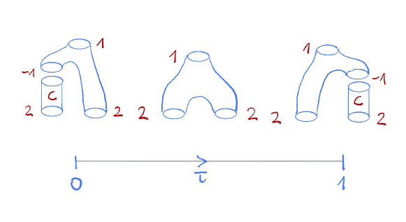
The coproduct . We fix a small vector field on with nondegenerate zeroes such that the only periodic orbits of with period are its zeroes. (The last property can be arranged, e.g., by choosing gradient-like near its critical points; then the periods of nonconstant periodic orbits are uniformly bounded from below by a constant , so has the desired property.) Denote by
the flow of , i.e. the solution of the ordinary differential equation . It follows that the only fixed points of are the zeroes of , each zero is nondegenerate as a fixed point, and
where is the index of as a zero of . The map
is transverse to the diagonal and
Since for the map , fills up the complement to , the induced orientation on endows with the sign .
Remark 2.8.
Alternatively, we could use the exponential map of some Riemannian metric to define a map by . Although this map differs from above, for sufficiently small it shares its preceding properties and could be used in place of .
Consider now a generic family of vector fields , which interpolates between and . We denote , the flow of and . Note that, while and have nondegenerate zeroes, this condition cannot be guaranteed for . Genericity of the family means that the maps , , and , , are transverse to the diagonal.
For each and we denote the induced path from to by
and the inverse path by
Recall from above the restriction and concatenation of paths. Now for we set
with
See Figure 1.
Note that the matching conditions imply . This is a codimension condition and, as the family is generic, is a transversely cut out manifold of dimension
If its dimension equals zero this manifold is compact and defines a map
If the dimension equals it can be compactified to a compact -dimensional manifold with boundary
Here the first three terms correspond to broken pseudo-gradient lines and the last two terms to the intersection of with the sets and , respectively. So we have
| (9) |
where for we set
Let us look more closely at the map . For the matching conditions in imply that is a fixed point of , the time-one flow of , and is the constant loop at . Assuming that has a unique minimum and the fixed points of are in general position with respect to the stable and unstable manifolds of , the condition is only satisfied for . Thus is empty if and
Choosing all fixed points of closely together, we can achieve that the terms on the right hand side corresponding to different are in canonical bijection to each other. By the discussion before Remark 2.8, the terms corresponding to a fixed point come with the sign . Since and we obtain
Since the last moduli space is the one in the definition of , we conclude
or equivalently
Similarly we have
or equivalently
In conclusion we obtain condition (4) in Definition 2.1,
We define the secondary continuation quadratic vector by
Condition (2), i.e. , follows by inserting into the relation for and using that is a strict two-sided unit for on . This is an instance of unital -structure [20]. Note that for energy reasons.
We now prove condition (5) in Definition 2.1. For it holds because , hence . We therefore assume w.l.o.g. and give the proof in two steps.
-
(1)
We first prove . This follows from , which is seen as follows. The coefficient can only be nonzero if are critical points of . Since has degree , we must have , hence . Since , this is impossible for .
-
(2)
We now show that , where . We identify with the Morse cochain complex . The cohomological index of is , so its components must have degrees and . If these degrees are both positive, and therefore any component of is killed by multiplication with because the latter has cohomological index .
In summary we have shown
Proposition 2.9.
Each vector field on satisfying the preceding conditions gives rise to a special -structure on the Morse complex of the functional .
Remark 2.10.
In the previous construction we used an interpolating family of vector fields such that . This choice is important because it ensures that the product on the Rabinowitz loop homology obtained from the -structure via the cone construction is associative, and much more: in view of the isomorphism with the -structure on symplectic homology proved in §6 and in view of [16, 20], the resulting product fits into a graded Frobenius algebra structure on .
While the construction of an -structure would have worked with any choice of nondegenerate vector fields and at the endpoints of the parametrizing interval, the necessity of the condition , which ensures these fine properties of the product, would become visible at chain level within a theory of -structures. The development of such a theory is a matter for further study.
Remark 2.11.
Remark 2.12.
Alternatively, we could define the loop coproduct using the spaces
Again the matching conditions imply , and is a transversely cut out manifold of dimension whose rigid counts define a map
A discussion analogous to that for shows that Proposition 2.9 also holds with in place of . The obvious homotopies between the loops and in the definition of and the loops and in the definition of provide a special morphism between and , where . We will use the restriction of the map to Morse chains modulo constants in the proof of Proposition 7.4.
3. -structure for symplectic homology
As in the previous section, let be a closed oriented manifold. We pick a Riemannian metric on and denote by its unit sphere resp. unit disc cotangent bundle. The latter is a Liouville domain whose completion is . Its symplectic homology is defined as the direct limit of the Floer homologies over Hamiltonians that are negative on and linear outside a compact see; see [19] for general background on symplectic homology. The goal of this section is to construct a special -structure on the chain complex underlying symplectic homology.
3.1. The continuation map
Recall from [19] that for Hamiltonians we have a continuation map , defined by counting Floer cylinders for an -dependent Hamiltonian which agrees with for small , with for large , and which satisfies . In this subsection we will describe the continuation map
for a smooth Hamiltonian of the form
for a convex function with and for large , with not in the length spectrum, and a potential which has a unique maximum and a unique minimum . For -periodic orbits of and of , the coefficient is given by the count of solutions of the Floer equation
| (10) |
converging to as and to as . Here is a nonincreasing smooth function which equals for small and for large . For action reasons the coefficient can only be nonzero if are constant solutions corresponding to critical points of on the zero section , in which case the solutions are -independent and the Floer equation becomes the Morse equation
| (11) |
The Fredholm index of this problem is
with equality iff for the maximum of . On the other hand, solutions of (11) are in one-to-one correspondence to points , where denotes the stable manifold of with respect to . This shows that the Fredholm problem given by (10) resp. (11) is degenerate.
To perturb it, we denote by the -skeleton, i.e. the union of the descending manifolds of critical points of index . We pick a -form on satisfying the following condition:
| (12) | All zeroes of are nondegenerate and lie in . |
It gives rise to the flow
generated by the vector field on ,
We pick a compactly supported function with and perturb equations (10) and (11) to
| (13) |
and
| (14) |
To understand solutions of the perturbed Morse equation, we choose such that on and . Then solutions of (14) are in one-to-one correspondence to points
where the intersection is taken in . By condition (12) this intersection is empty unless , in which case intersection points correspond to zeroes of and their signed count equals the Euler characteristic of . This shows that the only nontrivial term in the continuation map is
and the corresponding quadratic vector is given by
In particular, satisfies the closedness condition in Definition 2.1, and it is also symmetric . Note that this holds without any symmetry assumptions on the data such as or . Note also that, although the definition of on the chain level requires the choice of a pair consisting of a Morse function and a -form on subject to condition (12), the result does not depend on this choice. In contrast, the secondary continuation quadratic vector which we construct below may depend on this choice. See also §4.
3.2. The product and coproduct
The pair-of-pants product (of degree ) counts maps from a pair-of-pants satisfying a Floer equation with weights at the two positive punctures and weight at the negative puncture. The definition is entirely analogous to the one for the coproduct given below, without the additional parameter . It is well-known that is a chain map which is associative and graded commutative up to chain homotopy (see e.g. [3]), so condition (2) in Definition 2.1 holds.
The critical point is a constant orbit and is a cycle which is a two-sided unit for up to homotopy. The subcomplex generated by small action orbits is stable under and we can choose the auxiliary data such that is a strict unit for the restriction of to .
In [22] a secondary coproduct is defined in terms of continuation maps on the reduced symplectic homology of a large class of Weinstein domains which includes cotangent bundles. See also [16, 20]. In this subsection we recall its definition for ; we will call it the continuation coproduct and denote it by .
The definition in [16, 20] is described in terms of real parameters satisfying . For simplicity, we choose the parameters as and for some . We assume that and do not belong to the action spectrum of .
As before, we denote by the radial coordinate on . Let be a convex smoothing of the Hamiltonian which is zero on and equals outside . Then and are the corresponding Hamiltonians of slopes and , respectively.
Let be the -punctured Riemann sphere, where we view one puncture as positive (input) and the other two as negative (outputs). We fix cylindrical coordinates near the positive puncture and near the negative punctures. Consider a -form on which equals near the positive puncture and near the -th negative puncture ) for some . We say that has weights . We moreover require , which is possible iff
We consider maps satisfying the perturbed Cauchy-Riemann equation
Near the punctures this becomes the Floer equation for the Hamiltonians and , respectively, and the algebraic count of such maps defines a (primary) coproduct
which has degree and decreases the Hamiltonian action.
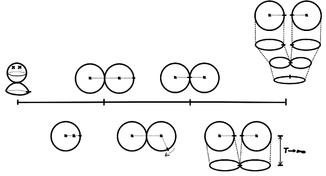
To define the secondary coproduct , we choose a -parameter family of -forms , , with the following properties (see Figure 2):
-
•
for all ;
-
•
equals near the positive puncture and near each negative puncture, i.e., has weights ;
-
•
as , equals on cylinders near the first negative puncture whose length tends to , so that consists of a -form on with weights and a -form with weights on an infinite cylinder attached at the first negative puncture;
-
•
as , equals on cylinders near the second negative puncture whose length tends to , so that consists of a -form on with weights and a -form with weights on an infinite cylinder attached at the second negative puncture.
Now we consider pairs where and satisfies the perturbed Cauchy-Riemann equation
The algebraic count of such pairs defines a (secondary) coproduct
which has degree and decreases the Hamiltonian action.
Let us analyze the contributions from . The algebraic count of cylinders with weights defines the continuation map (of degree )
As explained in the previous subsection, to define we perturb by a Morse function with a unique maximum at and a unique minimum at . Moreover, we choose a family of -forms on such that satisfies condition (12) (for all practical purposes one can think of as being constant). Finally, we choose a family of compactly supported -forms on which for agree with supported in the split off cylinder, for a function satisfying . For example, we can take where supported on the first negative end, and supported on the second negative end (below the level where the splitting happens at ). With the vector field on corresponding to , we replace the Cauchy-Riemann equation in the definition of by
| (15) |
With these choices, it follows from the discussion in the previous subsection that the only nontrivial terms in the continuation maps at are , where is the Euler characteristic of .
As shown in Figure 2, the contribution at consists of a pair-of-pants with one positive puncture of weight and two negative punctures of weights and , with a cylinder of weights and attached at the first negative puncture. We reinterpret this as a pair-of-pants with two positive punctures of weights and one negative puncture of weight , with a cylinder with two negative punctures of weights and attached at the first positive puncture. The preceding discussion shows that the count of these configurations corresponds to the composition . A similar discussion at establishes that satisfies condition (4) in Definition 2.1.
We define the secondary continuation quadratic vector by
Condition (2), i.e. , follows by inserting into the relation for and using that is a strict two-sided unit for on . This is an instance of unital -structure [20]. Note that for energy reasons. An inspection of the definition shows that coincides with the secondary continuation element defined in §4.2 by interpolating between the perturbing -form and its opposite . See also [22].
It remains to prove condition (5) in Definition 2.1. For it holds because , so that . We therefore assume w.l.o.g. and, as in the Morse case, we prove condition (5) in two steps.
-
(1)
We first prove . This follows from , which is seen as follows. For action reasons, the coefficient can only be nonzero if are critical points of . Since has degree , we must have , hence . Since , this is impossible for .
-
(2)
We are left to show that , where . We identify the Floer subcomplex generated by orbits of small action with the Morse cochain complex . The cohomological index of is , so its components must have degrees and . If these degrees are both positive, and therefore any component of is killed by multiplication with because the latter has cohomological index .
In summary we have shown
Proposition 3.1.
The operations on the Floer chain complexes resp. satisfy the relations of a special -structure.
The operations are compatible with Floer continuation maps between different Hamiltonians . We will refer to this structure as being the special -structure for symplectic homology .
Remark 3.2.
In the previous construction we imposed the condition at the endpoints of the family of -forms for the same reason why we imposed in the Morse case: this ensures that the product on Rabinowitz Floer homology obtained from the -structure via the cone construction coincides with the product from [16] and fits into a graded Frobenius algebra structure on .
The construction of an -structure would have worked with any choice of interpolating family such that and satisfy (12). The necessity of the condition for this fine behavior of the product would become visible at chain level within a theory of -structures.
4. Reduced loop homology
This section expands material from [22, §4] in the particular case of cotangent bundles. We assume that is connected and orientable, and we work either with constant coefficients on the loop space, or with local coefficients obtained by transgressing the 2nd Stiefel-Whitney class. In each of these two cases we have a commutative diagram
where the vertical maps are restriction to, resp. inclusion of constant loops, and is induced by multiplication with the Euler characteristic . From now on we omit from the notation the local system .
Definition 4.1.
We define reduced loop homology, resp. cohomology,
In the sequel we restrict the discussion to reduced homology. Reduced cohomology features similar properties, with the roles of the product and coproduct being exchanged (as yet another instantiation of Poincaré duality for loop spaces [16]).
The behavior of reduced homology with respect to the product is very robust. The image of is an ideal in (see for example [38] or [16]), and therefore the loop product canonically descends to reduced homology .
In contrast, the behavior of reduced homology with respect to the coproduct is very subtle. To describe it, the following variant of reduced loop homology arises naturally.
Definition 4.2.
We define loop homology relative to point as
A straightforward calculation shows that we have a canonical isomorphism
whenever the map is injective, see Appendix A.8. This is the case if is orientable and if we use a local system that is constant on the component of contractible loops, or if , or if is 2-torsion. We place ourselves from now on in this setup, so that we do not need to distinguish between and .
The loop coproduct is canonically defined on . We now explain that it always extends to (and hence to under our assumptions). However, this extension is not canonical. The extension depends on a choice of vector field with nondegenerate zeroes and on the choice of a Morse function on . We will completely describe the dependence of the extension on the choice of vector field, and give sufficient conditions for independence of the extension on the choice of Morse function.
4.1. Reduced symplectic homology
We work with symplectic homology of , our favorite model for loop space homology. Recalling notation from §3.1, we fix the following continuation data:
-
•
a Morse function with a unique maximum .
-
•
a -form on which satisfies condition (12), i.e., the zeroes of are nondegenerate and lie outside of (this is equivalent to a vector field on whose zeroes have the same property).
We consider Hamiltonians of the form , where and is a linear function of outside a compact set, of positive slope not belonging to the length spectrum. This data determines via equation (13) the Floer continuation map
which has the property that the only generator on which it may be nonzero is . Moreover, we have computed in §3.1 that
The continuation map can be equivalently interpreted as a quadratic vector
We emphasize that the chain level expression of the continuation map is the same for any choice of continuation data .
Definition 4.3.
The reduced Floer complex of is
Its homology is the reduced Floer homology of , denoted .
The reduced symplectic homology is the direct limit of reduced Floer homologies over Hamiltonians which vanish on and are linear outside a compact set, perturbed to have the form near the zero section as above. 222This group is strictly speaking the analogue of . In [22] we use the more precise notation and .
The relation
proved in §3.2, together with , shows that descends to a chain map . These maps are compatible with the continuation maps obtained by increasing the slope of , giving rise in the limit (with field coefficients) to a well defined coproduct of degree , denoted
A straightforward enhancement of the Viterbo-Abbondandolo-Schwarz isomorphism shows that the map induces an isomorphism between reduced homologies
In particular, associated to a choice of continuation data is a coproduct on . The key to understanding the dependence of the coproduct on the choice of continuation data is the secondary continuation map, which we describe next.
4.2. The secondary continuation map
Homotopies between different choices of pairs give rise to secondary operations which we describe in this subsection.
Consider two pairs , , satisfying the conditions of the previous subsection, i.e., is a Morse function with a unique maximum and a -form on such that condition (12) holds. For let be associated Hamiltonians as in the previous subsection. After shifting by constants we may assume without loss of generality that .
As in the previous subsection we pick a function which equals for and for . Let , , be a smooth family of -dependent Hamiltonians with the following properties:
-
•
for all ;
-
•
;
-
•
equals for and for ;
-
•
for and .
Let , , be a smooth family of -forms with for all . We consider pairs with and solving the Floer equation
and converging to -periodic orbits of as . Their algebraic count gives rise to a degree map
satisfying
| (16) |
with the Floer continuation maps for , , and . The map factors through the action zero part which we will denote by . Since the have unique maxima , it follows from the previous subsection that the only nontrivial contribution to is . Similarly, the only nontrivial contribution to the composition sends . This shows that the right hand side of equation (16) vanishes, and therefore descends to a map on homology
which factors through the action zero part
For degree reasons nontrivial contributions can only occur for and and give maps
In particular, we have shown
Proposition 4.4.
If , then the secondary continuation map associated to any interpolation between pairs , , of continuation data vanishes. ∎
4.3. Dependence of the continuation coproduct on choices
In this subsection we discuss the dependence of the continuation coproduct on the data of a Morse function and a -form on .
We consider the setup of the previous subsection and retain the terminology from there. Thus we are given two pairs , , with associated Hamiltonians satisfying . They give rise to Floer continuation maps , , and , and to a degree map satisfying equation (16).
We denote by the continuation coproducts (of degree ) defined with the data and families , such that as in §3.2. Let
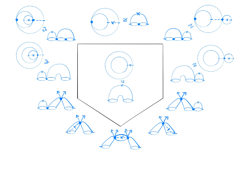
be the degree map defined by the -parametric family of Floer problems depicted in Figure 3.

These Floer problems are defined in terms of a -parametric family of Hamiltonian valued -forms on the -punctured sphere with asymptotics and degenerations as in the figure, and a -parametric family of -forms on which agree with , on the top side, with on the two top slanted sides, and with , on the bottom side of the hexagon.
On the reduced Floer chain complex the compositions along the top vertical sides vanish because they factor through the continuation map , so we obtain the relation
Here and are the degree operations appearing at the ends of the continuation coproduct as in Figure 2.
All the maps appearing on the right hand side of the last displayed equation are chain maps, so they descend to maps on reduced Floer homology (denoted by the same letters) satisfying
Passing to the direct limit over Hamiltonians as above, we have therefore shown
Proposition 4.5.
The continuation coproducts on defined with continuation data , , satisfy the relation
where is the secondary continuation map of the previous subsection and , are induced by the maps defined above. ∎
Remark 4.6.
The right hand side of the previous equation can be rephrased in terms of the secondary continuation map and the product . We refer to [22, §4.3] for further details.
Proposition 4.5 shows that in general the continuation coproduct may depend on the data . If , however, the secondary coproduct vanishes by Proposition 4.4 and we obtain
Proposition 4.7.
If , then the continuation coproduct on reduced symplectic homology is independent of the choice of continuation data . ∎
Remark 4.8.
In §3.2 we defined the coproduct using a family , with equal endpoints . The proof of Proposition 4.5 shows that, under the assumption , the coproduct can be defined using families with arbitrary endpoints satisfying condition (12) (in particular we can take ). This observation simplifies the computations in §8 for spheres of dimension by allowing the use of constant families of vector fields for the topological definition of the coproduct.
Corollary 4.9.
If then, denoting the unit and the canonical coproduct, we have .
A proof of this result in a more general setting is given in [22, §4], based on the vanishing of the secondary continuation map. We give here a topological proof, see also §8.2 for the case of spheres of odd dimension .
Proof.
We work on the topological side and compute, as in §8.2, the image of the fundamental class by representing it by constant loops and using a constant vector field with isolated nondegenerate zeroes. If has no zeroes then its image under the coproduct is zero because it is represented by the empty chain. In the general case the image is a degenerate -chain, hence vanishes in homology. ∎
5. Viterbo’s isomorphism revisited
As before, in this section is a closed oriented manifold, its cotangent bundle with the Liouville form , and its unit disc cotangent bundle viewed as a Liouville domain. The symplectic homology is isomorphic to the Floer homology of a fibrewise quadratic Hamiltonian . On the other hand, is isomorphic to the loop homology (Viterbo [39], Abbondandolo-Schwarz [1, 5], Salamon-Weber [35], Abouzaid [7]). Here we use coefficients twisted by the local system defined by transgressing the second Stiefel-Whitney class, cf. Appendix A. We drop the local system from the notation in the rest of this section.
The construction most relevant for our purposes is the chain map
from the Floer complex of a Hamiltonian to the Morse complex of an action functional on the loop space defined in [4]. When applied to a fibrewise quadratic Hamiltonian and the action functional associated to its Legendre transform , it induces an isomorphism on homology
intertwining the pair-of-pants product with the loop product [4].
One annoying feature of the map has been that, in contrast to its chain homotopy inverse , it does not preserve the action filtrations. This would make it unsuitable for some of our applications in [16] such as those concerned with critical values. Using an estimate inspired by [17], we show in this section that does preserve suitable action filtrations when applied to fibrewise linear Hamiltonians rather than fibrewise quadratic ones.
5.1. Floer homology
Consider a smooth time-periodic Hamiltonian which outside a compact set is either fibrewise quadratic, or linear with slope not in the action spectrum. It induces a smooth Hamiltonian action functional
Its critical points are -periodic orbits , which we can assume to be nondegenerate with Conley–Zehnder index . Let be a compatible almost complex structure on and denote the Cauchy–Riemann operator with Hamiltonian perturbation on by
Let be the free -module generated by and graded by the Conley–Zehnder index. The Floer differential is given by
where denotes the signed count of points in the oriented -dimensional manifold
Then and its homology is isomorphic to the symplectic homology if is quadratic. If is linear, we obtain an isomorphism to in the direct limit as the slope goes to infinity.
5.2. The isomorphism
Suppose now that is fibrewise convex with fibrewise Legendre transform . As in §2.2 we consider the Morse complex of the action functional
Following [1], for and we consider the space
where denotes the stable manifold for the pseudo-gradient flow of and is the projection. (It is sometimes useful to view as the unstable manifold for the negative pseudo-gradient flow of .) For generic this is a manifold of dimension
The signed count of -dimensional spaces defines a chain map
| (17) |
It was shown in [1] that the induced map on homology is an isomorphism
For consider the loop at . The definition of the Legendre transform yields the estimate
It follows that
whenever is nonempty, so decreases action.
5.3. The isomorphism
Consider once again a fibrewise quadratic Hamiltonian as in §5.2 with Legendre transform . Following [4, 17], for and we define
and
where is the stable manifold of for the negative pseudo-gradient flow of , see Figure 4.
For generic these are manifolds of dimensions
The signed count of -dimensional spaces defines a chain map
The induced map on homology is an isomorphism
which is the inverse of and intertwines the pair-of-pants product with the loop product. This was shown by Abbondandolo and Schwarz [4] with -coefficients, and by Abouzaid [7] (following work of Kragh [30], see also Abbondandolo-Schwarz [5]) with general coefficients, twisted on by a suitable local system, see Appendix A. Moreover, Abouzaid proved that is an isomorphism of twisted BV algebras.
Unfortunately, the map does not preserve the action filtrations. This already happens for a classical Hamiltonian : For the loop satisfies
so the middle inequality goes in the wrong direction (even if ).
5.4. An action estimate for Floer half-cylinders
Now we will replace the quadratic Hamiltonians from the previous subsections by Hamiltonians of the shape used in the definition of symplectic homology. For Floer half-cylinders of such Hamiltonians, we will estimate the length of their boundary loop on the zero section by the Hamiltonian action at .
We equip with a Riemannian metric and choose the following data.
The Riemannian metric on induces a canonical almost complex structure on compatible with the symplectic form (Nagano [32], Tachibana-Okumura [37], see also [11, Ch. 9]). In geodesic normal coordinates at a point and dual coordinates it is given by
We pick a nondecreasing smooth function with near and for large . Then
(in geodesic normal coordinates) defines a compatible almost complex structure on which agrees with near the zero section and is cylindrical outside the unit cotangent bundle.
We view as a function on . Then on we have
Consider a Hamiltonian of the form for a smooth function vanishing near . Then its Hamiltonian vector field equals , where is the Reeb vector field of . The symplectic and Hamiltonian actions of a nonconstant 1-periodic Hamiltonian orbit are given by
Given a slope which is not in the action spectrum of and any , we can pick with the following properties:
-
•
for and for , with some ;
-
•
and for .
Specifically, we choose , we consider a smooth function such that on , on and is strictly increasing on , and we define by
We have . This expression differentiates to and vanishes on , hence it is nonnegative for . On the other hand, we have an upper bound for , and indeed for . Given our choice , this establishes the inequalities for all .
These inequalities imply that for each nonconstant -periodic Hamiltonian orbit we have
| (18) |
With this choice of and , consider now as in the previous subsection a map satisfying
Set and denote its length by
The following proposition is a special case of [17, Lemma 7.2]. Since the proof was only sketched there, we give a detailed proof below.
Proposition 5.1.
Let be as above with and a nonconstant orbit . Then
The first inequality is an equality if and only if is contained in the half-cylinder over a closed geodesic , in particular is the lift of the geodesic .
The idea of the proof is to show that
Since the image can hit the zero section where is undefined, the quantity has to be interpreted as an improper integral as follows. Given , let be a smooth function with for all , near , and for , and consider the globally defined -form on given by
We now define
| (19) |
The proof of Proposition 5.1 is based on the following lemma.
Lemma 5.2.
For any , we have
At points where , equality only holds for , whereas at points where and equality holds if and only if is a linear combination of and .
Proof.
In geodesic normal coordinates we compute
For a vector of the form we obtain and hence by the Cauchy-Schwarz inequality
At points where , equality only holds for , and at points where and equality holds iff is a multiple of . Similarly, for a general vector we get , with equality iff either or and both and are multiples of . ∎
Proof of Proposition 5.1.
The proof consists in 3 steps.
Step 1. We prove that .
In view of Definition (19), it is enough to show that on all of . To see this, recall that satisfies the equation , so that
Now at points in the Hamiltonian vector field vanishes. At points outside we have and (we can assume w.l.o.g. ), so that . In either case we have
which is nonnegative by Lemma 5.2.
Step 2. Denote for . We have
To see this we consider the map
and denote as above for . Since near the zero section, the maps and agree with their first derivatives along the boundary loop at , hence and are -close for close to . On the other hand is -bounded near the zero section uniformly with respect to . These two facts imply that the integrals and are -close for close to , uniformly with respect to , and therefore
We now prove that
| (20) |
for all , which implies the desired conclusion. Fix therefore . Let , so that for and . On the one hand we have
We can therefore estimate
Here is the measure of , uniformly bounded by the length of the circle, is a -bound on near the -section, uniform with respect to , and is by definition the bound on on . The estimate follows from and the fact that the -form only acts on the first component of the vector .
Since , equality (20) follows.
Step 3. We prove
Indeed, for Stokes’ theorem gives
(The -form is equal to near the orbit .) The desired equality follows from the definition of and Step 2.
Conclusion. Combining Step 3 with Step 1 we obtain the first inequality in Proposition 5.1. Moreover, Lemma 5.2 (in the limit ) shows that this inequality is an equality if and only if is contained in the half-cylinder over a closed geodesic.
The second inequality follows from (18). ∎
5.5. The isomorphism from symplectic to loop homology
Now we adjust the definition of to symplectic homology. For as in the previous subsection and we define as before
By Proposition 5.1 the loop satisfies . Moreover, the loop is smooth and in particular has Sobolev class , hence following Anosov [10] it has a unique -reparametrization , with and (we say that is parametrized proportionally to arclength, or PPAL). We have
with the energy
The energy defines a smooth Morse-Bott function on the loop space whose critical points are constant loops and geodesics parametrized proportionally to arclength. We denote by the unstable/stable manifolds of with respect to . Now for and we define
An element in this moduli space still looks as in Figure 4, where now the loop is reparametrized proportionally to arclength and then flown into using the flow of . By Proposition 5.1, for we have the estimate
| (21) |
To define the map , we now perturb and by small Morse functions near the constant loops on and the closed geodesics, and we generically perturb the almost complex structure from the previous subsection. For generic such perturbations, each is a manifold of dimension
The signed count of -dimensional spaces defines a chain map
Here denotes the Morse chain complex of , graded by the Morse indices of , but filtered by the square root (which is decreasing under the negative gradient flow of ). The action estimate (21) continues to hold for the perturbed data up to an arbitrarily small error, which we can make smaller than the smallest difference between lengths of geodesics below a given length . Thus preserves the filtrations
The induced maps on filtered Floer homology
have upper triangular form with respect to the filtrations with on the diagonal (given by the half-cylinders over closed geodesics in Proposition 5.1), so they are isomorphisms. It follows from [4, 7] that intertwines the pair-of-pants product with the loop product, as well as the corresponding BV operators. Passing to the direct limit over Hamiltonians , we have thus proved
Theorem 5.3.
The map induces isomorphisms on filtered symplectic homology
where the left hand side is filtered by non-Hamiltonian action and the right hand side by the square root of the energy. These isomorphisms intertwine the pair-of-pants product with the Chas-Sullivan loop product, as well as the corresponding BV operators. ∎
6. Viterbo’s isomorphism intertwines -structures
We keep the setup from the previous section, so is a closed oriented Riemannian manifold and its unit disc cotangent bundle. In this section we prove Theorem 1.5, which will be an immediate consequence of earlier results and the following theorem.
Theorem 6.1.
The chain maps underlying the isomorphism
from Theorem 5.3 are morphisms of special -algebras. For these morphisms are special.
Proof of Theorem 1.5.
Remark 6.2 (open questions about the various identifications between Morse and Floer complexes for cotangent bundles).
We have already discussed in §5.2 the action preserving chain-level isomorphism of Abbondandolo-Schwarz [1], defined for an asymptotically quadratic Hamiltonian . It would be interesting to clarify whether also defines a morphism of special -algebras.
Abbondandolo-Schwarz constructed in [6] an action-preserving chain level isomorphism which is a chain homotopy inverse of . They also argued that, from the perspective of the Legendre transform, the moduli spaces that define arise naturally from the moduli spaces for . We expect that and our morphism can be connected by a suitable chain homotopy (we know that they induce the same map in homology). It would also be interesting to clarify whether is a morphism of special -algebras. We expect this to hold or fail for both and simultaneously.
One can further ask whether and are homotopic as morphisms of -structures. This would require in particular to develop the discussion of -structures from [20] by defining such a notion of homotopy.
To prove Theorem 6.1, we need to verify the conditions in Definition 2.3 for each chain map associated to a Hamiltonian as in the previous subsection. The first part of condition (i) holds because , which follows directly from the definition of . Moreover, seen through the canonical identifications , the restriction of to the energy zero Floer subcomplex acts as the identity. This shows that the second part of condition (i) is also satisfied.
The map in condition (ii) is defined by the count of elements in -dimensional moduli spaces of solutions to a -parametric mixed Floer-Morse problem which we describe below. Inspection of the boundary of the -dimensional moduli spaces of solutions shows that satisfies condition (ii). This fact was previously proved in [4], which contains the description of an essentially equivalent map .
The -parametric Floer-Morse problem is a count of Floer discs in with two positive punctures and boundary on the zero section, followed by a Morse pseudo-gradient line in the loop space of . It is obtained as a concatenation of 3 distinct -parametric Floer-Morse problems described by Figure 5. On the first interval of parametrization the underlying moduli space of curves is that of discs with 2 interior punctures and one boundary marked point, where the punctures and the marked point are requested to be aligned. At the negative end of the interval the 2 interior punctures collide and form a sphere bubble (this gives rise to the term in the expression of ), whereas at the positive end of the interval the second puncture collides with the marked point and gives rise to a disc bubble containing the marked point. In this configuration the interior punctures, the node and the marked point are all aligned. On the second interval of parametrization we allow the marked point to move clockwise towards the node. At the positive end of this interval the marked point collides with the node and forms a disc bubble. However, this disc bubble is constant because the 0-section is an exact Lagrangian, so that we directly replace the configuration by one where the marked point lies at the node. On the third and last interval of parametrization we insert length pseudo-gradient lines before imposing the incidence condition at the marked point. The positive end of this interval of parametrization corresponds to and gives rise to the term in the expression of .
In Figure 5 the dashed lines represent pseudo-gradient flow lines for the energy functional on loop space. We only represent them in the last two configurations depicted in Figure 5 in order not to burden excessively the drawing. However, the reader should be aware that such pseudo-gradient lines are also present in the first five configurations from Figure 5.
For further reference it is convenient to write
| (22) |
where , corresponds to the count of elements in the -dimensional moduli spaces of solutions to the Floer-Morse problem restricted to the -th interval of parametrization for .
The remainder of this section is devoted to the proof of condition (iii). For this we need to construct a chain homotopy
satisfying and
| (23) |
The map will be defined by a count of Floer maps to defined over a -parametric family of punctured annuli. In the first subsection we describe the underlying moduli space of conformal annuli.
6.1. Conformal annuli
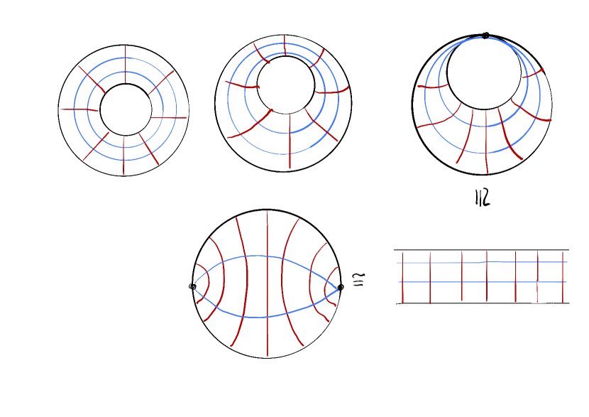
A (conformal) annulus is a compact genus zero Riemann surface with two boundary components. By the uniformization theorem (see for example [12]), each annulus is biholomorphic to with its standard complex structure for a unique called its (conformal) modulus. The exponential map sends the standard annulus onto the annulus
It will be useful to consider slightly more general annuli in the Riemann sphere . A circle in is the transverse intersection of with a plane. We will call a disc in an open domain bounded by a circle, and an annulus in a set for two discs satisfying (with the induced complex structure).
Lemma 6.3.
Every annulus in of conformal modulus can be mapped by a Möbius transformation onto the standard annulus above.
Proof.
Write for discs . After applying a Möbius transformation, we may assume that is the disc . Let be the unit disc. There exists a Möbius transformation of sending a point to a point and the positive tangent direction to at to the positive tangent direction to at . Thus sends to a circle tangent to at , and since the annuli and both have modulus we must have , hence . ∎
For each , the standard annulus carries two canonical foliations: one by the line segments and one by the circles . Moreover, these two foliations are invariant under the automorphism group of the annulus. Hence by Lemma 6.3 each annulus in also carries two canonical foliations, one by circle segments connecting the two boundary components and one by circles, such that the foliations are orthogonal and the second one contains the two boundary loops. These two foliations can be intrinsically described as follows: the automorphism group of an annulus is . The second foliation consists of the orbits of the -action. The first foliation is the unique foliation orthogonal to the first one. Its leaves connect the two boundary components because this is the case for a standard annulus.
Figure 6 shows a -parametric family of annuli in whose conformal moduli tend to together with their canonical foliations. The domain at modulus is the difference of two discs touching at one point, the node. Putting the node at the origin, the inversion maps this domain onto a horizontal strip in (with the node at ) with its standard foliations by straight line segments and lines. Opening up the node, we can conformally map it onto the standard disc with two boundary points corresponding to the node (since the map is not a Möbius transformation, the two foliations will not be by circle segments).
Annuli with aligned marked points. The relevant domains for our purposes are annuli with marked points, one interior and one on each boundary component. We require that the points are aligned, by which we mean that they lie on the same leaf of the canonical foliation connecting the two boundary components. (In the next subsection the interior marked point will correspond to the input from the Floer complex and the boundary marked points will be the initial points of the boundary loops on the zero section.)
Figure 7 shows the moduli space of such annuli with fixed finite conformal modulus. It is an interval over which the interior marked point moves from one boundary component to the other. Each end of the interval corresponds to a rigid nodal curve consisting of an annulus with one boundary marked point and a disc with an interior and a boundary marked point, where the marked point and the node are aligned in the annulus, and the two marked points and the node are aligned in the disc (i.e., they lie on a circle segment perpendicular to the boundary).
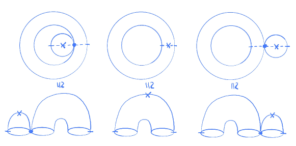
Figure 8 shows the moduli space of such annuli with varying conformal modulus. It is a pentagon in which we will view the two lower sides as being “horizontal” (although they meet at an actual corner). Then in the vertical direction the conformal modulus increases from (on the top side) to (on the two lower sides), while in the horizontal direction the interior marked point moves from one boundary component to the other. In all configurations the marked points and nodes are aligned. The interior nodes occuring along the bottom sides carry asymptotic markers (depicted as arrows) that are aligned with the boundary marked points. In particular, each interior node comes with an orientation reversing isomorphism between the tangent circles matching the asymptotic markers (this is the “decorated compactification”).
6.2. Floer annuli
Now we define a moduli space of Floer maps into over the moduli space of annuli in Figure 8. For this, we choose a family of -forms , , with the following properties (see Figure 9):
-
•
for all ;
-
•
equals near the (positive) interior puncture, and in coordinates near each (negative) boundary component, i.e., it has weights ;
-
•
on annuli of infinite modulus, has weights at the punctures (positive or negative) as shown in the figure.

In the figure the (black) bottom circles are boundary components, (blue) intermediate circles are interior punctures (viewed as positive or negative when going upwards or downwards), and (red) numbers denote the weights. Such a family exists because on each component of each broken curve the sum of negative weights is greater or equal to the sum of positive weights.
The annuli carry two marked points on their boundary circles (depicted as black dashes) which are aligned with the interior puncture. Again, all interior punctures carry asymptotic markers (not drawn) that are aligned with the boundary marked points, also over broken curves and are matching across each pair of positive/negative punctures.
Note that the bottom corner of the pentagon in Figure 8 has been replaced by a new side over which the underlying stable domain is fixed, but the weights at the positive/negative puncture vary as depicted with . Thus the conformal modulus is along the top side, and along the three bottom sides.
We fix a nonnegative Hamiltonian as in §3.2. For we denote by the corresponding (possibly broken) annulus with one positive interior puncture and two numbered boundary marked points on the boundary components , equipped with the -form . Given we define the moduli space
where the condition is understood as being -convergence as in cylindrical coordinates near the positive puncture . By Anosov [10], the restriction can be uniquely parametrized over as an -curve proportionally to arclength such that time corresponds to the marked point , . Viewing with these parametrizations thus yields a boundary evaluation map
Note that this map is also canonically defined over the boundary of . Indeed, this is clear everywhere except possibly over the two vertical sides where one boundary loop is split into two. There one component of is an annulus without interior puncture, on which the map is therefore constant (see the next subsection). Hence in the split boundary loop one component is constant, and we map it simply to the other component parametrized proportionally to arclength.
The expected dimension of is
where is the Euler characteristic of the punctured annulus. However, the moduli space is not transversely cut out over the vertical sides of . Indeed, the moduli space of non-punctured annuli appearing there has Fredholm index , where is the Euler characteristic of the annulus and the corresponds to the varying conformal modulus. But the actual dimension of this space is , where is the dimension of the space of constant maps . In the following subsections we explain how to achieve transversality by perturbing the Floer equation by a section in the obstruction bundle.
6.3. Moduli problems and obstruction bundles
To facilitate the discussion in the next subsection, we introduce in this subsection a general setup for moduli problems and obstruction bundles. Our notion of a moduli problem will be a slight generalization of that of a -moduli problem in [18] for the case of the trivial group , which allows us to work with integer rather than rational coefficients.
A moduli problem is a quadruple with the following properties:
-
•
is a Banach fibre bundle over a Banach manifold;
-
•
is a Banach submanifold transverse to the fibres;333In particular, is a closed subspace which has a closed complement for all .
-
•
is a smooth section such that the solution set
is compact and for each the composed operator
is Fredholm with constant index , and its determinant bundle
is oriented.
A morphism between moduli problems and is a pair with the following properties:
-
•
is a smooth embedding;
-
•
is a smooth injective bundle map covering such that
Moreover, the linear operators and induce for each isomorphisms
such that the resulting isomorphism from to is orientation preserving.
Proposition 6.4.
Each moduli problem has a canonical Euler class
Moreover, if is a morphism between moduli problems and , then and
Proof.
This follows directly from the corresponding results in [18]. To construct the Euler class, we compactly perturb to a section which is transverse to ; then is a compact manifold of dimension which inherits a canonical orientation and thus represents a class in , and it is easy to see that this class is independent of the choice of perturbation. The assertion about morphisms is obvious. ∎
A special case of a moduli problem arises if is a Banach vector bundle and is the zero section in . In this case is the vertical differential of at and we arrive at the usual notion of a Fredholm section. This is the setup considered in [18]; the general case can be reduced to this one (via a morphism of moduli problems) by passing to the normal bundle of .
Consider now a moduli problem such that
-
(i)
is a smooth submanifold, and
-
(ii)
for each .
Then the cokernels fit together into the smooth obstruction bundle
whose rank is related to the Fredholm index of by
We thus obtain a finite dimensional moduli problem , where denotes the zero section and its graph.
Lemma 6.5.
In the preceding situation there exists a canonical morphism of moduli problems
where is the inclusion and is a fibrewise exponential map.
Proof.
Choose a smooth Banach vector bundle such that for each ,
Since represents the normal bundle to in , we can assume that takes values in and is a subbundle of complementary to . Pick a fibrewise Riemannian metric on whose exponential map restricts to a fibre preserving embedding
Now it is easy to check that with the inclusion defines a morphism . ∎
In the situation of Lemma 6.5, the Euler class of is therefore represented by the zero set of a section in the obstruction bundle which is transverse to the zero section. Concretely, keeping the notation from the proof, defines a section of the fibre bundle . We extend the bundle to a bundle on a neighbourhood of and to a section of the bundle vanishing near the boundary of . Then the perturbed section of is transverse to and its solution set represents the Euler class of .
Remark 6.6 (orientations).
In the situation of Lemma 6.5 we are given an orientation of
| (24) |
Let now be a section transverse to the zero section. Its zero set is a submanifold and at each the linearization is surjective with kernel , so we get a canonical isomorphism of line bundles
Combined with (24) this yields a canonical isomorphism
so an orientation of induces an orientation of . In the case this can be made more explicit as follows. Then and an orientation of induces an isomorphism
For we define the sign to be if the isomorphism preserves orientations, and otherwise. Then the signed count
is the Euler number of the obstruction bundle .
Finally, consider a moduli problem which splits as follows:
-
•
;
-
•
;
-
•
for sections such that is transverse to .
Lemma 6.7.
In the situation above there exists a reduced moduli problem
and a morphism of moduli problems from to, with the inclusion and .
Proof.
Since is transverse to , it follows that is a submanifold and defines a moduli problem. Now it follows directly from the definitions that as in the lemma induces for the canonical identities
hence it defines a morphism of moduli problems. ∎
6.4. Constant Floer annuli
In this subsection we apply the results of the previous subsection to moduli spaces of annuli. We begin with a rather general setup. Let be a compact Riemann surface with boundary, and be an almost complex manifold with a half-dimensional totally real submanifold . For and with we consider the Banach manifold
and the Banach space bundle whose fibre over is
Denote the zero section. The Cauchy-Riemann operator
defines a Fredholm section . Assuming a setup in which the space of solutions is compact (e.g. if is tamed by an exact symplectic structure on , the totally real submanifold is exact Lagrangian, and has a compact group of automorphisms), we obtain a moduli problem .
Constant annuli of positive modulus. Now we apply the preceding discussion to the moduli space of constant annuli appearing in the previous subsection. Consider a fixed annulus of finite conformal modulus , equipped with a -form as above satisfying and in cylindrical coordinates near the two (negative) boundary loops. Let be the nonnegative Hamiltonian from §3.2. Then the Floer operator defines a Fredholm section in the appropriate bundle over the Banach manifold
We denote its zero set by . For the usual energy estimate (see e.g. [34]) gives
where the Hamiltonian action of vanishes because both the Liouville form and the Hamiltonian vanish on the zero section . This implies that . Since vanishes near the zero section, it follows that near and therefore, by unique continuation, is constant equal to a point in . Hence the moduli space
consists of points in , viewed as constant maps . Since vanishes near the zero section, the Floer operator agrees with the Cauchy-Riemann operator near , so we can and will replace by in the following discussion of obstruction bundles.
We identify with the standard annulus and its trivial tangent bundle . Consider a point , viewed as a constant map . We identify
Then we have
where for the last equality we use the canonical isomorphism
With these identifications, the linearized Cauchy-Riemann operator reads
An easy computation using Fourier series (see [14]) shows that
So the Cauchy-Riemann operator, and thus the Floer operator, satisfies conditions (i) and (ii) in the previous subsection with the obstruction bundle
and Lemma 6.5 implies
Corollary 6.8.
In the preceding situation there exists a canonical morphism of moduli problems
where is the inclusion as constant maps and converts a cotangent vector into a constant -form. ∎
Note in particular that has index zero. A section in the obstruction bundle transverse to the zero section corresponds under the isomorphism to a -form on with nondegenerate zeroes , and the zero set of the perturbed Floer operator consists of viewed as constant maps . Having chosen the orientation of to be induced by the canonical isomorphism , we obtain that the signed count
agrees with the Euler number of . Note that the Euler number of equals the Euler characteristic of (this follows from the canonical isomorphism and the Poincaré-Hopf theorem).
Constant annuli of modulus zero. Annuli of conformal modulus zero can be viewed as moduli problems in two equivalent ways. For the first view, we take as domain the compact region bounded by two circles touching at one point, the node. Given and as above, we therefore obtain a moduli problem with
the Cauchy-Riemann operator , and the zero section .
For the second view, we take as domain the closed unit disk with viewed as nodal points which are identified. This gives rise to a moduli problem with
Note that the indices of the two moduli problems agree,
Let be a continuous map which maps onto the nodal point and is otherwise one-to-one, and which is biholomorphic in the interior.444We may construct as a composition where is the Möbius transformation sending onto the upper halfplane with and , is the logarithm sending onto the strip , and is the Möbius transformation sending onto . Then composition with defines a diffeomorphism
(where we use as area form on the pullback under of an area form on ). Since is transverse to the diagonal , we are in the situation of Lemma 6.7. We conclude that there exists a morphism of moduli problems
where is the inclusion and .
Now we specialize to the case with its canonical almost complex structure . Then both solution spaces and consist of constant maps to . Moreover, in view of the preceding discussion and the fact that the Cauchy-Riemman operator over the disk is transverse to the zero section, they both satisfy the hypotheses (i) and (ii) of Lemma 6.5, so combined with the preceding discussion we obtain
Corollary 6.9.
There exists a commuting diagram of morphisms of moduli problems
where and are the inclusions as constant maps, the bundle is given by projection onto the first factor, and is the composition of the isomorphism induced by a metric on with the exponential map . Thus the Euler class of each of these moduli problems is represented by the nondegenerate zeroes of a -form on (or equivalently, of a vector field on ), with signs that add up (up to a global sign) to the Euler characteristic of . ∎
6.5. Proof of Theorem 6.1
Now we can conclude the proof of Theorem 6.1.
For consider the moduli space of Floer annuli described in §6.2 with its boundary evaluation map . Pick a -form on with nondegenerate zeroes . As in §6.4, we view as a section of the obstruction bundle over the vertical sides of the hexagon in Figure 9. We extend this section by a cutoff function to a section over the whole hexagon and add it as a right hand side to the Floer equation. We choose the data such that the moduli space is transversely cut out, and thus defines a compact manifold with corners of dimension .
We may assume without loss of generality that is connected. We pick a -small Morse function with a unique maximum at such that flow to under the positive gradient flow of . Let denote the Morse complex of the perturbed energy functional
(note that there is no factor in front of ). For and we define
where is the stable manifold of with respect to the negative pseudo-gradient flow of . Recall that the boundary evaluation map involves reparametrization of the boundary loops proportionally to arclength. For generic choices, these are manifolds of dimension
If the dimension is these spaces are compact and their signed counts
define a degree map
Next we consider a -dimensional moduli space and compute its boundary. Besides splitting off index Floer cylinders and negative pseudo-gradient flow lines, which give rise to the term , there are contributions from the sides of the hexagon in Figure 9 which we analyze separately. Note that the indices now satisfy
Vertical left side: Here the broken curves consist of a half-cylinder attached at a boundary node to an annulus without interior puncture, where the two boundary loops flow into under the negative pseudo-gradient flow of . By the discussion in §6.4 the moduli space of annuli is , where encodes the conformal modulus and consists of the points (with signs ). In particular, we must have and therefore . The half-cylinders belong to the moduli space
They carry a boundary nodal point which is aligned with the boundary marked point and the puncture at , and is therefore given by . The evaluation at the nodal point defines an evaluation map
For the broken curve to exist this evaluation map must meet one of the constant annuli, i.e. one of the points , which generically does not happen because
Hence the vertical left side gives no contribution to the boundary.
Vertical right side: Similarly, the vertical right side gives no contribution to the boundary.
Lower left side: Here the broken curves consist of a disc with two interior punctures, one positive and one negative, attached at its negative puncture to the positive puncture of a half-cylinder along an orbit in , where the two boundary loops flow into under the negative pseudo-gradient flow of . By choosing the -form equal to on a long cylindrical piece of the half-cylinder, we can achieve that these half-cylinders are in one-to-one correspondence with broken curves consisting of a cylinder with weights and a half-cylinder with weights , as shown in the middle of Figure 10. Reinterpreting these curves as on the right of that figure, we see that their count corresponds to the composition , where we recall that denotes the first term in the expression from (22).
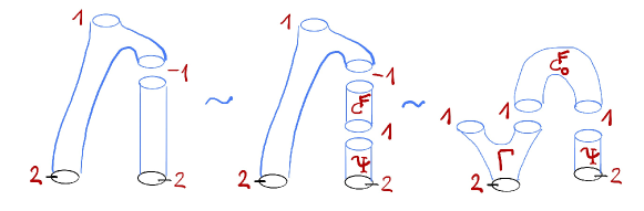
Lower right side: Similarly, the contribution from the lower right side corresponds to the composition .
The discussion so far shows that
| (25) |
where and are the degree maps arising from the contributions of the top and bottom sides of the hexagon to the boundary of which we discuss next.
Bottom side: The family of broken curves on the bottom side can be deformed in an obvious way to the family of broken curves shown in Figure 11. Since the half-cylinders with weights define the map and the family of 3-punctured spheres above them defines the continuation coproduct from §3.2, this shows that is equal to .
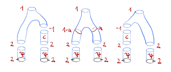
Top side: The family on the top side of the hexagon consists of punctured annuli of modulus , i.e., punctured discs with two nodal points on the boundary that are identified to a node. Moreover, the boundary carries two marked points that are separated by the nodal points and aligned with the interior puncture. We wish to relate this family to the loop coproduct, but for this we face two problems: First, the boundary loops carry two marked points whereas the loops for the loop coproduct carry only one (the initial time ); and second, the self-intersection of the boundary loop occurs at the nodal points and not at one of the marked points.
Both problems are resolved simultaneously as follows. We enlarge this -parametric family to a -parametric family in which we keep the two boundary marked points aligned, but drop the condition that the interior puncture is aligned with them. The -parametric family forms the hexagon shown in Figure 12. Here the interior puncture is depicted as a cross, the aligned boundary marked points as endpoints of a dashed line, and the nodal points as thick dots. The bottom side of the hexagon (drawn in black) corresponds to the -parametric family on the top side of Figure 9. Note that here we made a choice by letting the interior puncture move freely above the dashed line connecting the two boundary marked points; we could equally well have taken the mirror hexagon where the interior puncture moves below the dashed line.
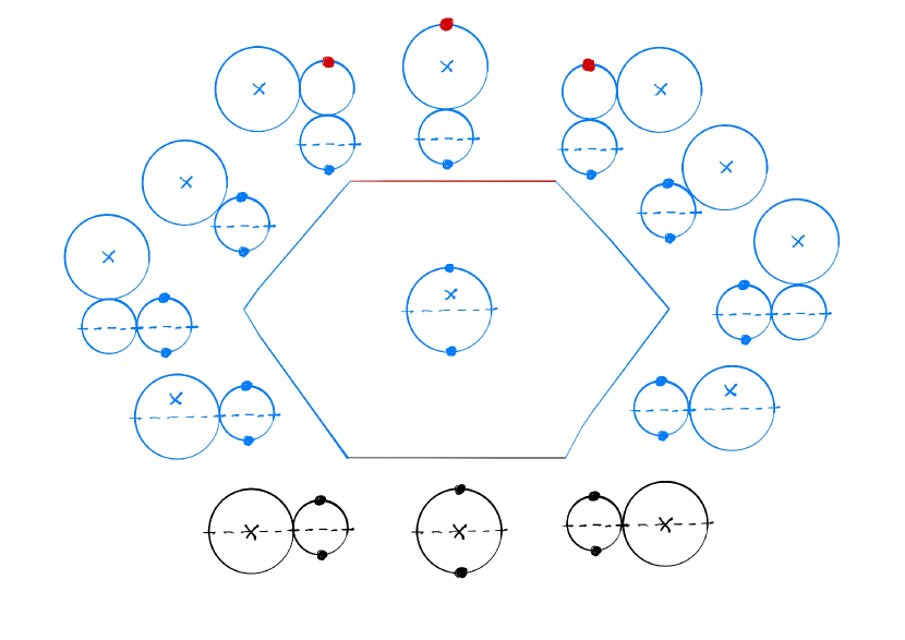
The hexagon in Figure 12 defines a deformation from the bottom (black) side to the top side (drawn in red). The configurations in this figure are to be interpreted as follows.
Each configuration has two boundary loops obtained by going around in the counterclockwise direction: the first loop from the bottom to the top nodal point, and the second one from the top to the bottom nodal point. Each boundary loop carries a marked point. As before, each boundary loop of the zero section is reparametrized proportionally to arclength and then flown into a critical point on under the negative pseudo-gradient flow of the functional .
In each configuration the unique component carrying the interior puncture (which may be nonconstant) is drawn as a large disc, so the small discs are all constant. In particular, each small disc carrying the two nodal points is a constant annulus of modulus zero. Under the perturbation of the Cauchy-Riemann equation described in Corollary 6.9, such a component lands on the transverse zeroes of a -form and further flows into the basepoint . In particular, since the signs add up to we have that all configurations on the upper and lower left sides land in , while those on the upper and lower right sides land in . The upper and lower left sides therefore compute , whereas the lower and upper right sides compute , with being the second term in (22).
Thus the hexagon in Figure 12 provides a chain homotopy from (defined by the bottom side) to the operation , where is defined by the top side, i.e.
| (26) |
Consider now the top side. Since both marked points and the black nodal point lie on the same constant component, we can remove this component and replace the three points by one nodal/marked point as shown in Figure 13.
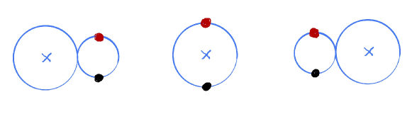
The boundary of these configurations consists of loops with one (black) marked/nodal point at time and an additional (red) nodal point at time which moves from to as we traverse the side from left to right. In view of Corollary 6.9 and Remark 6.6, the map is defined by counting isolated configurations consisting of punctured discs as in the definition of the moduli spaces from §5.5, additionally decorated with two marked points, with an incidence condition at the marked points, followed by semi-infinite negative pseudo-gradient lines of starting at the de-concatenated loops. Now we deform once more by inserting a negative pseudo-gradient trajectory of of finite length between the boundary loop of the disc and the loop on which we impose the incidence condition at the marked points. As this becomes the chain map followed by the Morse theoretic coproduct , whereas on the boundary of the top side we see appear the terms , with being the third term from (22). We obtain therefore a homotopy between the operation defined by the top side and , i.e.
| (27) |
Summing together equations (25), (26) and (27), and recalling that , we obtain the desired relation (23).
For , the condition follows by an index argument analogous to the proof of the relation in Proposition 3.1. Together with the discussion at the beginning of this section, this concludes the proof of Theorem 6.1. ∎
Remark 6.10 (Perturbation by -form/vector field).
Let us analyze how the perturbation by a -form with transverse
zeroes propagates to the diagrams in the preceding proof.
Along the left hand sides of the hexagon in Figure 9,
we perturb the Floer operator by at the second output.
This continues along the left hand sides of the hexagon in
Figure 12 as the perturbation of the constant
modulus zero annuli by the vector field corresponding to
at the second output.
As a result, the left hand configuration in Figure 13
is perturbed by applying the time-one-map of as we go
counterclockwise from the black to the red dot.
This means for close to the evaluations of the corresponding loops
at time (the black dot) and (the red dot) are related by .
Along the right hand sides of the hexagon in Figure 9,
we perturb the Floer operator by at the first output.
As a result, the right hand configuration in Figure 13
is perturbed by applying the time-one-map of as we go
clockwise from the black to the red dot.
This means that for close to the evaluations of the corresponding loops
at time (the black dot) and (the red dot) are related by
, or equivalently, .
Therefore, the perturbation by the -form on the Floer side
translates on the loop side into the perturbation by an -dependent
vector field which agrees with near and with near .
7. Relation to other Floer-type coproducts
The continuation coproduct discussed in the previous sections descends to positive action symplectic homology (since the action inequality implies that if the input orbit is constant, then so must be the output orbits). In this section we relate to other coproducts on that have appeared in the literature, thus proving Theorem 1.1 from the Introduction.
In particular, we will prove that agrees with the Abbondandolo–Schwarz coproduct defined in [4]. Abbondandolo and Schwarz defined in [4] the ring isomorphism and they asserted [4, Theorem 1.4] that its reduction modulo constant loops intertwines the coproduct with the loop coproduct . However, to our knowledge no proof of this result has appeared. We will actually give two proofs in this section: the first one uses Theorem 6.1 and the identification , the second one uses a direct argument and suitable interpolating moduli spaces.
This section is structured as follows. In §7.1 we recall from [20] the definition of the varying weights coproduct , which coincides with by [20, Lemma 7.2] and which can be more easily related to . In §7.2 we recall from [4] the definition of the Abbondandolo–Schwarz coproduct . In §7.3 we show that is equal to . In §7.4 we prove directly that corresponds to the loop coproduct under the isomorphism .
The situation is summarized in the following diagram.
| (28) |
The whole discussion concerns the free loop space, but it carries over verbatim to the based loop space.
For simplicity, we assume throughout this section that is oriented and we use untwisted coefficients in a commutative ring ; the necessary adjustments in the nonorientable case and with twisted coefficients are explained in Appendix A. We denote
7.1. Varying weights coproduct
We recall the definition of the varying weights coproduct on from [20, §7.1]. Since there we actually describe the algebraically dual product on , we will recap in some detail the necessary notation and arguments. The construction goes back to Seidel, see also [26]. We work with a Liouville domain of dimension , the symplectic completion is denoted and the radial coordinate in the positive symplectization is denoted .
Let be the genus zero Riemann surface with three punctures, one of them labeled as positive and the other two labeled as negative , , endowed with cylindrical ends at the positive puncture and at the negative punctures. Denote , the induced cylindrical coordinates at each of the punctures. Consider a smooth family of -forms , satisfying the following conditions:
-
•
(nonpositive) ;
-
•
(weights) near each of the punctures;
-
•
(interpolation) we have on in the cylindrical end near , and on in the cylindrical end near , for some smooth function . In other words, the family interpolates between a -form which varies a lot near and very little near , and a -form which varies a lot near and very little near ;
-
•
(neck stretching) we have as .
We can assume without loss of generality that for close to we have in the cylindrical end at the negative puncture , with , near , and on , and similarly for close to in the cylindrical end at the negative puncture .
Let be a convex smoothing localized near of a Hamiltonian which is zero on and linear with respect to with positive slope on . The Hamiltonian further includes a small time-dependent perturbation localized near , so that all -periodic orbits are nondegenerate. Assume the slope is not equal to the period of a closed Reeb orbit. Denote the set of -periodic orbits of . The elements of are contained in a compact set close to .
Let , , be a generic family of compatible almost complex structures, independent of and near the punctures, cylindrical and independent of and in the symplectization . For denote
In the symplectization we have and therefore , so that elements of the above moduli space are contained in a compact set. The dimension of the moduli space is
When it has dimension zero the moduli space is compact. When it has dimension the moduli space admits a natural compactification into a manifold with boundary
Here and denote the fibers of the first projection , near , respectively near . (By a standard gluing argument the projection is a trivial fibration with finite fiber near the endpoints of the interval .)
Consider the degree operation
defined on generators by
where denotes the signed count of elements in the -dimensional moduli space . Consider also the degree operations
defined on generators by
where denotes the signed count of elements in the -dimensional moduli space .
Denote by the Floer differential on the Floer complex of . The formula for translates into the algebraic relation
| (29) |
We now claim that
To prove the claim for , note that this map can be expressed as a composition , where is a pair-of-pants coproduct with small, and is a continuation map. Taking into account that has no nontrivial -periodic orbits for small, and because the action decreases along continuation maps, we obtain , which proves the claim. The argument for is similar.
It follows that induces a degree chain map
| (30) |
Passing to the limit as the slope of goes to we obtain the degree varying weights coproduct on .
Proposition 7.1 ([20, Lemma 7.2]).
The continuation coproduct and the varying weights coproduct coincide on :
∎
7.2. Abbondandolo–Schwarz coproduct
In this subsection we recall from [4] the definition of a secondary pair-of-pants product on Floer homology of a cotangent bundle, which we will refer to as the Abbondandolo–Schwarz coproduct . We recall the notation and conventions from §5.1 regarding the Floer complex. In particular near the zero section for a small and a Morse function such that all nonconstant critical points of have action larger than .
Lemma 7.2 ([4, §5]).
For generic choices of Hamiltonian and almost complex structure the space is a transversely cut out manifold of dimension
∎
The dimension of is calculated in [4] using an equivalent description of the moduli space as follows. Define by and , and also by and . Then there is a canonical identification between elements of and elements of
Here is the antisymplectic involution , is the diagonal, and its conormal bundle. The space is a moduli space with jumping Lagrangian boundary conditions as in [3], so for generic and it is a transversely cut out manifold. Its dimension is given by the Fredholm index of the linearized problem [4, (37)].
If has dimension zero it is compact and defines a map
If it has dimension it can be compactified to a compact -dimensional manifold with boundary
Here the first three terms correspond to broken Floer cylinders and the last two terms to the intersection of with the sets and , respectively. Therefore we have
| (31) |
where for we set
Let us look more closely at the map . For the matching conditions in imply that is a constant loop. For action reasons must then be a critical point, so that . Similarly we have , and therefore descends to a chain map
| (32) |
with . Note that we have for the quadratic Hamiltonians considered in this section.
7.3. The varying weights coproduct equals the Abbondandolo–Schwarz coproduct
Proposition 7.3.
Proof.
We assume without loss of generality that the Hamiltonian used in the definition of the coproduct is the same as the one used in the definition of the coproduct , i.e. a convex smoothing of a Hamiltonian which vanishes on and is linear with respect to the radial coordinate outside of . The point of the proof is to exhibit the Floer problem defining the moduli spaces for as a limiting case of the Floer problem defining the moduli spaces for .
Note first that for -dimensional moduli spaces we can restrict to . Given a triple as in the definition of can be interpreted as a single map satisfying , where is a Riemann surface and is a -form explicitly described as follows. The Riemann surface is
with
(We use the notation for points in , and for points in .) This is a smooth Riemann surface with canonical cylindrical ends at the positive puncture and and at the negative punctures. See Figure 15.
A conformal parametrization of near the point is induced from the map , . 555Consider the half-pair-of-pants , where for . A conformal parametrization near is given by the map defined in a neighborhood of . This map actually establishes a global conformal equivalence between and . The Riemann surface admits a natural presentation as the gluing of two copies of . Accordingly, it can be identified to where the equivalence relation stands for suitable identifications of boundary components. The map defined in a neighborhood of provides a conformal parametrization of near the point . The Riemann surface carries a canonical smooth closed -form . 666Read through the identification of with , this is in a neighborhood of . Upon identifying the cylindrical ends at the negative punctures with , this canonical -form becomes equal to , respectively at those punctures. The -form is defined to be the discontinuous -form equal to on the cylindrical end at the positive puncture, equal to on the cylindrical end at the first negative puncture, and equal to on the cylindrical end at the second negative puncture. Equivalently, upon normalizing the cylindrical ends at the negative punctures into , the -form is simply . This discontinuous -form can be interpreted as a limit of -forms which are obtained by interpolating from and (near ) towards (near ) in the normalized cylindrical ends at the negative punctures, where the interpolation region shrinks and approaches . It was noted in §7.2 that the limit case defines a Fredholm problem with jumping Lagrangian boundary conditions. The Fredholm problem before the limit is naturally phrased in terms of the Riemann surface without boundary, but it can be reinterpreted as a problem with Lagrangian boundary conditions by cutting open along . As such, it converges in the limit to the Fredholm problem with jumping Lagrangian boundary conditions described above. By regularity and compactness, the two Fredholm problems are equivalent near the limit, and the corresponding counts of elements in -dimensional moduli spaces are the same. ∎
7.4. Abbondandolo–Schwarz coproduct equals loop coproduct
Recall the Hamiltonian from §7.2 and its fibrewise Legendre transform from §2.2. Also recall from §2.2 the notations concerning the Morse complex of the action functional which we will use freely. In particular, denotes the Morse boundary operator and the coproduct from Remark 2.12.
We assume that is oriented and we use the Morse complex twisted by the local system obtained by transgressing the second Stiefel-Whitney class.
Following [4], for and we define
and
| (33) |
where is the stable manifold of for the negative pseudo-gradient flow of . See Figure 4.
For generic these are manifolds of dimensions
The signed count of -dimensional spaces defines a chain map
The induced map on homology is an isomorphism
intertwining the pair-of-pants product with the loop product.
Proposition 7.4.
The map descends to an isomorphism on homology modulo the constant loops
which intertwines the Abbondandolo–Schwarz coproduct with the loop coproduct .
Proof.
For and define
where was defined above and for denotes the flow of the negative pseudo-gradient of . Note that in the definition of are actually redundant and just included to make the definition more transparent. As above it follows that for generic these spaces are transversely cut out manifolds of dimensions and
We set
If this space has dimension zero it is compact and defines a map
If it has dimension it can be compactified to a compact -dimensional manifold with boundary
where are the moduli spaces in Remark 2.12 defining the coproduct with . Here the first term corresponds to splitting off of Floer cylinders, the second and third ones to splitting off of Morse pseudo-gradient lines, the fourth one to , the fifth one to , and the last two terms to the intersection of with the sets and , respectively. The intersections of with the set are equal with opposite orientations and thus cancel out. Therefore we have
| (34) |
where for we set
Arguing as in the previous subsection, we see that the has image in , and has image in . Together with equation (34) this shows that descends to a map
between the positive chain complexes which is a chain homotopy between and , which concludes the proof. ∎
8. Loop coproduct for odd-dimensional spheres
In this section we compute the loop coproduct on reduced loop homology of odd-dimensional spheres . For its definition we use a Morse function with only two critical points, the minimum and the maximum, and a vector field (or equivalently a -form ) which is nowhere vanishing. By Proposition 4.7, the coproduct does not depend on these choices if . For the same reason, in the definition of the loop coproduct we can use a constant family instead of the family interpolating between and from §2.2 (see Remark 4.8). In the case we will see that the loop coproduct actually depends on the choice of .
For our computation we first give a third definition of the loop coproduct on reduced loop homology in terms of singular homology.
8.1. Topological description of the loop coproduct
We define the loop coproduct on singular loop homology relative to point. It is induced by a densely defined operation
on singular chains constructed as follows. The beginning of the construction is like in §2.2. We fix a small vector field on with nondegenerate zeroes such that the only periodic orbits of with period are its zeroes, and we consider a generic family of vector fields , which interpolates between and . We denote , the flow of , and . For each we denote as in §2.2 the induced path from to by , , and the inverse path by .
In the spirit of [13], let be a chain such that the map
is transverse to the diagonal . Then
is a compact manifold with corners and we define
by
See Figure 1 where . At and the condition in becomes , respectively , and denoting the constant loop at by the same letter we find
It follows that
where is viewed as a -chain and the loop products with the constant loop are given by
Here the signs arise from the discussion before Remark 2.8, noting that the restriction of to or is the composition of the evaluation , and the map , , respectively .
Let us now fix a basepoint and consider such that the map
is transverse to . We choose all zeroes of (i.e. fixed points of and ) so close to that is transverse to each of them. Then after identifying the domains with and transferring loops at to loops at we have
| (35) |
where is the Euler characteristic of . Recalling the notation for the chains relative to point, we see that induces a chain map . Moreover, this factors through : if this holds for degree reasons, and if this holds tautologically because the Euler characteristic is zero. The outcome is a coproduct on the homology relative to point. Under our standing assumption of orientability on , this is the same as a coproduct on reduced loop homology .
8.2. Loop coproduct for spheres of odd dimension
In this subsection we use -coefficients and assume is odd. Recall from [23] that the degree shifted homology of the free loop space of is the free graded commutative algebra
where the shifted degree is related to the geometric degree by . Here is the class of a point (of geometric degree ) and is represented by the descending manifold of the Bott family of simple great circles tangent at their basepoint to a given non-vanishing vector field on the sphere (of geometric degree ). Since , the coproduct is defined on and has shifted degree (and geometric degree ). The unit is represented by the fundamental chain of all constant loops (of geometric degree ).
We begin with some explicit computations of coproducts, to be compared to [29].
Lemma 8.1.
For odd, the loop coproduct on satisfies
(a) ,
(b) ,
(c) ,
(d) .
Proof.
We will actually prove these relations in , in which case (a-c) remain unchanged, but (d) becomes (the sign change comes from the odd degree shift by ).
We recall the observation made at the beginning of this section that in the definition of the loop coproduct we can use a constant family of vector fields . We fix such a choice in the sequel, with small and nowhere vanishing. We denote the flow of , and we denote the time one flow.
(a) To prove we represent by the constant loop at . Then for all values of and therefore is supported by the empty set. To prove we represent by the -family of constant loops and note that for all . Thus is supported by the empty set.
(b) We fix a unit tangent vector at and we represent by the -chain of all circles with fixed initial point and initial direction . ( is the -disc of all -planes in through containing the vector , whose boundary is mapped to .) Then for all . Since the evaluation map covers once, there exists a unique for which . Therefore, is homologous to the -cycle .
(c) We represent by the -chain of all circles with fixed initial point . ( is a fibre bundle , where is the -sphere of all initial directions at and is the -disc from (b) of all circles through in a given initial direction.) Then for all . Recall that is a point close to . Let us fix some initial direction at . For every sufficiently large circle (whose diameter is bigger than the distance from to ) with initial point and initial direction there exist precisely two rotations of the initial direction such that the rotated circles pass through . One of these rotated circles passes though near and the other one near . As the circle varies over the -chain of all circles with initial point and initial direction (and we let move to ), these two families of rotated circles give rise to cycles representing the classes and , respectively.
(d) We represent by the -chain of all circles starting at their basepoint in direction . ( is a fibre bundle , where corresponds to the initial points and is the -disc from (b).) For every there exists a unique circle starting at in direction and passing through . Since all the circles constituting the chain are simple, there is a unique such that . By splitting each at the parameter value using the path we obtain a cycle that represents . This cycle has degree , it sits over the diagonal as an element of the fibration , and denoting the restriction of this fibration to the diagonal we have . On the other hand, has rank , generated by the class of the diagonal: that the rank is at most follows by inspection of the spectral sequence of the fibration , using the fact that is a polynomial ring on one generator in degree , and that it is at least one follows from the fact that the diagonal is a section. This implies that the cycle is homologous to the diagonal in , hence also in , and we conclude in .
The previous proof uses an algebraic argument related to the diagonal. An alternative, entirely geometric proof can be given in case the sphere admits two orthogonal non-vanishing vector fields. (By Adams’ theorem [8], this is the case if and only is divisible by .) We pick to be one of these and denote the other one. We represent by the -chain of all circles starting at their basepoint in direction . Thus for every there exists a unique circle starting at in direction and passing through , and since all the circles constituting the chain are simple there is a unique such that . Since is orthogonal to , each circle is small and the resulting cycle can be deformed in to the diagonal . In turn, this is represented in by , i.e. . ∎
Note that Lemma 8.1 is compatible with graded cocommutativity of on , i.e. . To compute the full expression of the coproduct we use the following structural result from [22].
Theorem 8.2 ([22, Theorem 6.4]).
Let be a closed manifold of dimension . Then the loop homology endowed with the loop product and the loop coproduct is a commutative and cocommutative unital infinitesimal anti-symmetric bialgebra. In particular, the following “unital infinitesimal relation” holds:
where we denote the identity map and the unit for the product. ∎
For with odd we proved in Lemma 8.1 that , so the unital infinitesimal relation reduces to the so-called “infinitesimal relation”, or “Sullivan relation”
Such a relation was conjectured in [36]. Note that Sullivan’s relation is not satisfied by the “extension by ” loop coproduct from [29].
Proposition 8.3.
For odd, the loop coproduct on satisfies for all
Proof.
The proof is a straightforward induction on using knowledge of , Sullivan’s relation, and the values and from Lemma 8.1. As an example, the values of and from Lemma 8.1 can be recovered as follows. For the computation, recall that the shifted degrees of , , are odd, the shifted degree of is even, and .
∎
Remark 8.4.
We note in particular that this extended coproduct on reduced homology has contributions from the constant loops, unlike the one from [29]. These contributions from the constant loops play an essential role for the unital infinitesimal algebra structure.
The previous computation allows us to recover the Sullivan-Goresky-Hingston coproduct on [29, 27]. Our method ultimately relies on the infinitesimal relation and involves a minimal geometric input in the form of Lemma 8.1 (a) and (d). In comparison, the computation from [29] of the coproduct on relies on geometric input which is quite involved. In a sense, the “algebra” of the infinitesimal relation replaces the “geometry” of spaces of circles from [29].
Corollary 8.5.
For odd, the Sullivan-Goresky-Hingston coproduct on is given by
Proof.
It is enough to discard the terms involving constant loops from the formulas of Proposition 8.3. ∎
8.3. Loop coproduct for
In this section we study the loop coproduct on the loop space of . The degree shifted loop homology with -coefficients is as a ring with respect to the loop product given by
where the classes and are represented by the cycles
To define the loop coproduct (of shifted degree ), we need to pick a nowhere vanishing vector field on . Up to homotopy there are two choices of nonvanishing vector fields on ,
for some fixed small . We associate to the -dependent vector fields
which agree with at and with at . Their time-one maps are
In the next Proposition we compute the coproducts associated to this choice of -dependent vector fields.
Proposition 8.6.
The loop coproducts on defined with the -dependent vector fields are given for by
Proof.
Let us compute . By definition, we need to determine the times such that
i.e. with . In other words, we are looking for the such that
For we obtain
while for we get
This yields the expressions for , and is computed similarly. ∎
Proposition 8.6 shows that for the coproduct on reduced loop homology does depend on the choice of a nowhere vanishing vector field. One can verify that both coproducts define together with the loop product a commutative cocommutative infinitesimal anti-symmetric bialgebra in the sense of [22] with
The unital infinitesimal relation reads now
Remark 8.7.
Just like in the case of higher-dimensional spheres, the expressions of the coproducts on can be derived from the unital infinitesimal relation combined with knowledge of the product and of the values
For example, to compute one applies the unital infinitesimal relation to , to compute one applies the unital infinitesimal relation to (or to ) etc.
Remark 8.8.
The example of the circle is very rich in that it also shows that the condition for the family of vector fields is necessary in order for the coproducts to have a good algebraic behaviour. For example, with a constant family we find an operation given by
A direct check shows that this operation is neither coassociative, nor cocommutative, though it satisfies the unital infinitesimal relation with , i.e. Sullivan’s relation. Similarly, with the constant family we find an operation given by
Again, this is neither coassociative, nor cocommutative, though it satisfies Sullivan’s relation.
Appendix A Local systems
We describe in this section the loop product and the loop coproduct with general twisted coefficients. This allows us in particular to dispose of the usual orientability assumption for the underlying manifold. To the best of our knowledge, the Chas-Sullivan product on loop space homology was constructed for the first time on nonorientable manifolds by Laudenbach [31], and the BV algebra structure by Abouzaid [7]. In this appendix we extend the definitions to more general local systems, we take into account the coproduct, and we discuss the adaptations to reduced homology and cohomology groups and . We also discuss the formulation and properties of the isomorphism between symplectic homology and loop homology with twisted coefficients.
A.1. Conventions.
We use the following conventions from [7, §9.7]. Given a finite dimensional real vector space , its determinant line is the -dimensional real vector space . We view it as being a -graded real vector space supported in degree . To any -dimensional graded real vector space we associate an orientation line , which is the rank graded free abelian group generated by the two possible orientations of , modulo the relation that their sum vanishes. The orientation line is by definition supported in the same degree as . When we denote its orientation line .
Given a -graded line (rank free abelian group), its dual line is by definition supported in opposite degree as . There is a canonical isomorphism induced by evaluation.
Given a -graded object , we denote the -graded object obtained by shifting the degree down by , i.e. . For example, the shifted orientation line is supported in degree . A linear map between -graded vector spaces or free abelian groups has degree if for all . In an equivalent formulation, the induced map has degree . For example, the dual of a vector space or free abelian group supported in degree is supported in degree . This is compatible with the grading convention for duals of -graded orientation lines. Given a -graded rank free abelian group , we denote the same abelian group with degree set to . For example .
Given two oriented real vector spaces and , we induce an orientation on their direct sum by defining a positive basis to consist of a positive basis for followed by a positive basis for . This defines a canonical isomorphism at the level of orientation lines
Given an exact sequence of vector spaces
we induce an orientation on out of orientations of and by defining a positive basis to consist of a positive basis for followed by the lift of a positive basis for . This defines a canonical isomorphism
The following example will play a key role in the sequel.
Example A.1 (normal bundle to the diagonal).
Let be a manifold of dimension . Consider the diagonal and denote its normal bundle. Let be the projections on the two factors, so that we have a canonical isomorphism . When restricted to the projections coincide with the canonical diffeomorphism . We obtain an exact sequence of bundles
This gives rise to a canonical isomorphism and, because is canonically trivial, we obtain a canonical isomorphism
Explicitly, this isomorphism associates to the equivalence class of a basis , of the equivalence class of the basis of .
A.2. Homology with local systems
By local system we mean a local system of -graded rank free -modules. On each path-connected component of the underlying space we think of such a local system in one of the following three equivalent ways: either as the data of the parallel transport representation of the fundamental groupoid, or as the data of the monodromy representation from the fundamental group to the multiplicative group together with the data of an integer (the degree), or as the data of a -graded -module which is free and of rank as a -module. Isomorphism classes of local systems on a path connected space are thus in bijective correspondence with , where the first factor corresponds to the monodromy representation and the second factor to the grading. Here and in the sequel we identify the multiplicative group with the additive group . We refer to [9] for a comprehensive discussion with emphasis on local systems on free loop spaces. One other point of view on local systems describes these as locally constant sheaves, but we will only marginally touch upon it in §A.3.
Given a local system , we can change the coefficients to any commutative ring by considering . The monodromy of such a local system still takes values in , and this property characterizes local systems of rank free -modules which are obtained from local systems of rank free -modules by tensoring with .
Let be a path connected space admitting a universal cover . Denote its fundamental group at some fixed basepoint . Interpreting a local system on as a -module, one defines singular homology/cohomology with coefficients in in terms of singular chains on as
The homology/cohomology with local coefficients extended to a commutative ring are the -modules
In our grading convention the cohomology with constant coefficients is supported in nonpositive degrees and equals the usual cohomology in the opposite degree. The induced differential on the dual group has degree .
The tensor product of two local systems is again a local system. Its -module structure is the diagonal one and its degree is the sum of the degrees of the factors. Note that viewing as elements in , their tensor product is given by their sum . Operations like cap or cup product naturally land in homology/cohomology with coefficients in the tensor product of the coefficients of the factors.
Homology/cohomology with local coefficients behave functorially in the following sense. Given a continuous map and a local system on described as a -module, the pullback local system on is defined by inducing a -module structure via . We then have canonical maps
The algebraic duality isomorphism with coefficients in a field takes the form
The map is induced by the canonical evaluation of cochains on chains. We check that degrees fit in the case of graded local systems: given a local system of degree , and recalling our notation and , we have
so and both live in degree .
A.3. Poincaré duality
Consider a manifold of dimension . We denote by the local system on whose fiber at any point is the orientation line , supported by definition in degree . We refer to as the orientation local system of . The monodromy along a loop is if the loop preserves the orientation (i.e., the pullback bundle is orientable), and if the loop reverses it. The local system is trivial if and only if the manifold is orientable. A choice of orientation is equivalent to the choice of one of the two possible isomorphisms . The local system is trivial, and this reflects the fact that any manifold is -orientable.
Suppose now that is closed. Then it carries a fundamental class .
For any local system on , the cap product with a fundamental class defines a Poincaré duality isomorphism
Remark A.2.
Here is a description of the fundamental class using the interpretation of local systems as locally constant sheaves (see for example [28], Lemma 3.27 and Example 3H.3). Let be the orientation double cover. Given the constant local system on , the pushforward to has rank and can be decomposed as (the map , fixes the diagonal and acts by on the anti-diagonal). The composition is an isomorphism because is an isomorphism. Since if is nonorientable, we obtain that has rank . A generator is the image of a generator in via the above composition.
A.4. Thom isomorphism and Gysin sequence
Let be a real vector bundle of rank , and denote the complement of the zero section. Let be the local system on whose fiber at a point is the orientation line of the fiber of at . The local system is called the orientation local system of and is supported in degree . The Thom class is a generator
The Thom isomorphism takes the form
(cap product with ), respectively
(cup product with ). More generally, for any local system on we have isomorphisms
Pulling back the Thom class under the inclusion of the zero section yields the Euler class
Denote by the sphere bundle with projection . Then the long exact sequence of the pair fits into the commuting diagram
where the lower sequence is the Gysin sequence. More generally, for each local system on we get a Gysin sequence
A.5. Spaces of loops with self-intersection
Let be a manifold of dimension , its space of free loops of Sobolev class , and the evaluation of loops at time . We define
(pairs of loops with the same basepoint), and
(loops with a self-intersection at time ). Denoting , and , , we can equivalently write
The maps and are smooth and transverse to the diagonal , so that and are Hilbert submanifolds of codimension . Denoting and their normal bundles we obtain canonical isomorphisms
In view of Example A.1 we infer canonical isomorphisms
| (36) |
where, in the first formula, is the evaluation of pairs of loops at their common origin.
Denote and the inclusions. Recall the restriction maps (7). Define the cutting map at time
and the concatenation map at time
The maps and are smooth diffeomorphisms inverse to each other. The situation is summarized in the diagram
Lemma A.3.
Let be a local system (of rank free abelian groups) on supported in degree . Denote the projections on the two factors. The following two conditions are equivalent:
| (37) |
and
| (38) |
Proof.
The first condition is . Since is a homeomorphism, this is equivalent to
In view of , this is the same as the second condition. ∎
Definition A.4.
A degree local system on is compatible with products if it satisfies the equivalent conditions of Lemma A.3.
A local system which is compatible with products must necessarily have degree (and rank ). Also, must be trivial: restricting both sides of (37) or (38) to the constant loops yields .
Remark A.5.
Local systems which are compatible with products play a key role in the sequel definition of the loop product and loop coproduct with local coefficients. Condition (37) is the one that ensures the coproduct is defined with coefficients twisted by , whereas condition (38) is the one that ensures the product is defined with coefficients twisted by . That the two conditions are equivalent can be seen as yet another instance of Poincaré duality for free loops.
Example A.6 (Transgressive local systems).
Let be the decomposition of the free loop space into connected components, indexed by conjugacy classes in the fundamental group. We view loops as maps , . This induces a map , . Dually, and specializing to -coefficients, any cohomology class determines a cohomology class via
We denote the corresponding local system on also by . Degree local systems obtained in this way are called transgressive [7].
Transgressive local systems are compatible with products. Indeed, the identity (38) is a direct consequence of the equality , which holds in for all .
The transgressive local system
| (39) |
defined by the second Stiefel-Whitney class will play a special role in the sequel.
Example A.7.
Following Abouzaid [7], define for each loop the shift
Define the local system
| (40) |
to be trivial on the components where preserves the orientation, and equal to on components where reverses the orientation.
The local system is compatible with products: the equality holds in for all . Note that the local system is not transgressive and, in case is nonorientable, it is nontrivial on all connected components whose elements reverse orientation.
Question A.8.
A.6. Loop product with local coefficients
Following [27], we view the loop product as being defined by going from left to right in the diagram
where for some fixed . More precisely, the loop product with integer coefficients is defined as the composition
The first map is the homology cross-product corrected by a sign ([29, Appendix B]), the second map is the composition of the map induced by inclusion with excision and the tubular neighbourhood isomorphism, and the third map is the Thom isomorphism. In case is not orientable the loop product does not land in homology with integer coefficients and thus fails to define an algebra structure on . This can be corrected by using at the source homology with local coefficients.
Definition A.9.
Define on the local system
The archetypal loop product is the bilinear map
defined as the composition
The description of the maps is the same as above, with because of the shift . However, one still needs to check that the local systems of coefficients are indeed as written. For the first, second and third map the behavior of the coefficients follows general patterns. For the last map we use that
which is true for our specific .
The archetypal loop product is associative, graded commutative, and it has a unit represented by the fundamental class
from §A.3. With our grading conventions, the archetypal loop product has degree and the local system is supported in degree . In the case where is oriented we recover the usual loop product.
More generally, the loop product can be defined with further twisted coefficients.
Definition A.10.
Let be a degree local system (of rank free -modules) on which is compatible with products. The loop product with coefficients twisted by is the bilinear map
(with as above) defined as the composition
As before, we have . For the last map we use the isomorphism , and the isomorphism which expresses the compatibility with products for .
The loop product with twisted coefficients is graded commutative and unital. Recalling that the compatibility with products for forces its restriction to to be trivial, the unit is again represented by the fundamental class
Remark A.11.
Associativity of the loop product with twisted coefficients depends on the following associativity condition on the isomorphisms (37) and (38). Given denote , so that . Denoting the isomorphism from (38), we require the associativity condition
This holds for the transgressive local systems from Example A.6 and for the local system in Example A.7.
A.7. Loop coproduct with coefficients
Again following [27], we view the primary coproduct on loop homology as being defined by going from left to right in the diagram
for some fixed , where stands for in the notation of §A.5. We restrict in this section to coefficients in a field and all local systems are accordingly understood in this category. The reason for this restriction is explained below. The primary coproduct with constant coefficients is defined as the composition
The first map is the composition of the map induced by inclusion with the excision isomorphism towards the homology rel boundary of a tubular neighbourhood of . The second map is the Thom isomorphism. For the third map we use that . The fourth map is the Alexander-Whitney diagonal map followed by the Künneth isomorphism.777The Alexander-Whitney diagonal map [25, VI.12.26] takes values in with arbitrary coefficients. In order to further land in we need to restrict to field coefficients so the Künneth isomorphism holds. Alternatively, one needs to modify the target of the coproduct to be , see [29]. Just like for the loop product, we see that if is nonorientable the primary coproduct fails to define a coalgebra structure on . This is corrected by using homology with local coefficients as follows.
Definition A.12.
Define on the local system
The archetypal primary coproduct is the bilinear map
(for some fixed ) defined as the composition
With our grading conventions this coproduct has degree . Taking into account that is supported in degree , this results in the coproduct having the usual degree in ungraded notation. In the orientable case it recovers the usual primary coproduct.
Just like the product, the primary coproduct can be defined with further twisted coefficients.
Definition A.13.
Let be a degree local system (of rank one -vector spaces) on which is compatible with products. The primary coproduct with twisted coefficients is the bilinear map
(with as above and some fixed ) defined as the composition
In the definition we use , and the condition which is part of the condition of being compatible with products for .
The arguments of Goresky-Hingston [27, §8] which show that, in the orientable case, there is a secondary coproduct of degree defined on relative homology , apply verbatim in the current setup involving local coefficients. As an outcome, we obtain the following.
Definition-Proposition A.14.
For any degree local system of rank one -vector spaces on which is compatible with products, there is a well-defined (secondary) loop coproduct with twisted coefficients (abbreviate )
∎
As explained in [29], in order for this secondary coproduct to be coassociative in the case of a constant local system we need to correct the -component of the secondary product induced by the previously defined primary product by a sign (see [29, Definition 1.7] and note the shift in grading ). With this correction the coproduct with constant local system is also graded cocommutative if gradings are shifted so that it has degree . However, it has no counit (this would contradict the infinite dimensionality of the homology of ).
In the case of coefficients twisted by a local system which is nonconstant, coassociativity further requires that the isomorphisms expressing compatibility with products for satisfy the condition from Remark A.11. The coproduct is then also cocommutative.
One obtains dually a cohomology product [27, 29]. Note that, in contrast to the loop coproduct, the dual loop cohomology product is defined with arbitrary coefficients because its definition does not require the Künneth isomorphism.
Definition-Proposition A.15.
For any degree local system of rank free abelian groups on which is compatible with products, there is a well-defined cohomology product with twisted coefficients (abbreviate )
∎
The cohomology product with twisted coefficients is associative. It is also graded commutative when viewing it as a degree product on .
A.8. Reduced- vs. loop homology relative to point
We explain in this section the interplay between reduced loop homology and loop homology relative to point in the presence of local coefficients.
Recall the previous notation , and let be a local system compatible with products. The arguments of §2.2 carry over verbatim to give a description of the loop product and coproduct in Morse homology with local coefficients in , respectively . For a definition of Morse homology with local coefficients we refer to [7, §11.3] or [33, §7.2].
The reduced loop (co)homology groups and are defined with local coefficients as follows. Recall that is trivial. We consider the map given as the composition
where the vertical maps are restriction to, respectively inclusion of constant loops, and is induced by multiplication with the Euler characteristic. We then define
Thus and . Similarly to §2.2, the loop product descends to because is an ideal.
The loop (co)homology groups relative to point are defined with local coefficients as follows. Recall again that is trivial. Consider the embedding given by the inclusion and define the Morse chains relative to point as . Similarly consider the projection and define the Morse cochains relative to point to be . The loop (co)homology groups relative to point are
The arguments of §2.2 carry over verbatim in order to show that the loop coproduct extends to (for algebraic reasons we need to use field coefficients as in §A.7). Interpreted dually as a product on cohomology, this is defined with arbitrary coefficients on .
The comparison between reduced loop homology and loop homology relative to a point goes as follows. Recalling that , we have a commutative diagram
which induces
We thus get a canonical map
| (41) |
which is an isomorphism if and only if the map is injective. To study its injectivity we can restrict without loss of generality to the component of contractible loops, in which case the target of this map is if is trivial and if is nontrivial on that component. We thus obtain injectivity of this map, and an isomorphism in (41), under any of the following conditions:
(i) is trivial on the component of contractible loops.
(ii) .
(iii) is -torsion.
A.9. Isomorphism between symplectic homology and loop homology
We spell out in this section the isomorphism between the symplectic homology of the cotangent bundle and the homology of the free loop space with twisted coefficients.
For the next definition, recall the local systems
from (39) and (40), as well as the orientation local systems
Definition A.16 (Abouzaid [7]).
The fundamental local system for symplectic homology of the cotangent bundle is the local system on given by
The fundamental local system is supported in degree . Our previous discussion shows that the loop product is defined and has degree on , and the loop coproduct is defined and has degree on . We can view the loop product as being defined on , where it has degree , and the loop coproduct as being defined (with field coefficients) on , where it has degree . This point of view is useful when considering , which is a common space of definition (to which the product descends and the coproduct extends).
As proved in [5, 7], the chain map discussed in §5.3 associated to a quadratic Hamiltonian acts as
and induces an isomorphism . Given any local system , the same map acts as and induces an isomorphism .
Our filtered chain map from §5.5 associated to a linear Hamiltonian is a chain isomorphism , with the slope of the Hamiltonian. Given any local system , we obtain a filtered chain isomorphism .
In case the local system is compatible with products, the arguments of [1, 3, 7] adapt in order to show that the map intertwines the pair-of-pants product on the symplectic homology side with the homology product on the Morse side. The arguments of Theorem 6.1 adapt in order to show that the map descends on homology relative to the constant loops, where it intertwines the continuation coproduct with the loop coproduct (with field coefficients).
Theorem A.17 ([1, 3, 5, 7], Theorem 5.3, Theorem 6.1).
Given any local system compatible with products, the filtered chain level map induces filtered isomorphisms
Moreover:
– intertwines the pair-of-pants product with the Chas–Sullivan loop product,
– intertwines the continuation coproduct with the loop coproduct (with field coefficients). ∎
There are also reduced versions of the map which intertwine the product, and which also intertwine the coproducts provided both are defined using the same continuation data at the endpoints. The statements for the coproducts can moreover be interpreted as dual statements about products in cohomology.
References
- [1] A. Abbondandolo and M. Schwarz. On the Floer homology of cotangent bundles. Comm. Pure Appl. Math., 59(2):254–316, 2006.
- [2] A. Abbondandolo and M. Schwarz. A smooth pseudo-gradient for the Lagrangian action functional. Adv. Nonlinear Stud., 9(4):597–623, 2009.
- [3] A. Abbondandolo and M. Schwarz. Floer homology of cotangent bundles and the loop product. Geom. Topol., 14(3):1569–1722, 2010.
- [4] A. Abbondandolo and M. Schwarz. On product structures in Floer homology of cotangent bundles. In Global differential geometry, volume 17 of Springer Proc. Math., pages 491–521. Springer, Heidelberg, 2012.
- [5] A. Abbondandolo and M. Schwarz. Corrigendum: On the Floer homology of cotangent bundles. Comm. Pure Appl. Math., 67(4):670–691, 2014.
- [6] A. Abbondandolo and M. Schwarz. The role of the Legendre transform in the study of the Floer complex of cotangent bundles. Comm. Pure Appl. Math., 68(11):1885–1945, 2015.
- [7] M. Abouzaid. Symplectic cohomology and Viterbo’s theorem. In Free loop spaces in geometry and topology, volume 24 of IRMA Lect. Math. Theor. Phys., pages 271–485. Eur. Math. Soc., Zürich, 2015.
- [8] J. F. Adams. Vector fields on spheres. Ann. of Math. (2), 75:603–632, 1962.
- [9] P. Albers, U. Frauenfelder, and A. Oancea. Local systems on the free loop space and finiteness of the Hofer-Zehnder capacity. Math. Ann., 367(3-4):1403–1428, 2017.
- [10] D. V. Anosov. Some homotopies in a space of closed curves. Izv. Akad. Nauk SSSR Ser. Mat., 44(6):1219–1254, 38, 1980.
- [11] D. E. Blair. Riemannian geometry of contact and symplectic manifolds, volume 203 of Progress in Mathematics. Birkhäuser Boston, Ltd., Boston, MA, second edition, 2010.
- [12] P. Buser. Geometry and spectra of compact Riemann surfaces. Modern Birkhäuser Classics. Birkhäuser Boston, Ltd., Boston, MA, 2010. Reprint of the 1992 edition.
- [13] M. Chas and D. Sullivan. String topology. arXiv:math/9911159, 1999.
- [14] K. Cieliebak. Pseudo-holomorphic curves and periodic orbits on cotangent bundles. J. Math. Pures Appl. (9), 73(3):251–278, 1994.
- [15] K. Cieliebak, U. Frauenfelder, and A. Oancea. Rabinowitz Floer homology and symplectic homology. Ann. Sci. Éc. Norm. Supér. (4), 43(6):957–1015, 2010.
- [16] K. Cieliebak, N. Hingston, and A. Oancea. Poincaré duality for loop spaces. arXiv:2008.13161, 2020.
- [17] K. Cieliebak and J. Latschev. The role of string topology in symplectic field theory. In New perspectives and challenges in symplectic field theory, volume 49 of CRM Proc. Lecture Notes, pages 113–146. Amer. Math. Soc., Providence, RI, 2009.
- [18] K. Cieliebak, I. Mundet i Riera, and D. A. Salamon. Equivariant moduli problems, branched manifolds, and the Euler class. Topology, 42(3):641–700, 2003.
- [19] K. Cieliebak and A. Oancea. Symplectic homology and the Eilenberg–Steenrod axioms. Algebr. Geom. Topol., 18(4):1953–2130, 2018.
- [20] K. Cieliebak and A. Oancea. Multiplicative structures on cones and duality. arXiv:2008.13165, 2020.
- [21] K. Cieliebak and A. Oancea. CoFrobenius bialgebras, Poincaré duality, and graded TQFT. arXiv:2209.02979, 2022.
- [22] K. Cieliebak and A. Oancea. Reduced symplectic homology and the secondary continuation map. arXiv:2209.02972, 2022.
- [23] R. L. Cohen, J. D. S. Jones, and J. Yan. The loop homology algebra of spheres and projective spaces. In Categorical decomposition techniques in algebraic topology (Isle of Skye, 2001), volume 215 of Progr. Math., pages 77–92. Birkhäuser, Basel, 2004.
- [24] R. L. Cohen and M. Schwarz. A Morse theoretic description of string topology. In New perspectives and challenges in symplectic field theory, volume 49 of CRM Proc. Lecture Notes, pages 147–172. Amer. Math. Soc., Providence, RI, 2009.
- [25] A. Dold. Lectures on algebraic topology, volume 200 of Grundlehren der Mathematischen Wissenschaften [Fundamental Principles of Mathematical Sciences]. Springer-Verlag, Berlin-New York, second edition, 1980.
- [26] T. Ekholm and A. Oancea. Symplectic and contact differential graded algebras. Geom. Topol., 21(4):2161–2230, 2017.
- [27] M. Goresky and N. Hingston. Loop products and closed geodesics. Duke Math. J., 150(1):117–209, 2009.
- [28] A. Hatcher. Algebraic topology. Cambridge University Press, Cambridge, 2002.
- [29] N. Hingston and N. Wahl. Product and coproduct in string topology. arXiv:1709.06839, 2017.
- [30] T. Kragh. The Viterbo transfer as a map of spectra. J. Symplectic Geom., 16(1):85–226, 2018.
- [31] F. Laudenbach. A note on the Chas-Sullivan product. Enseign. Math. (2), 57(1-2):3–21, 2011.
- [32] T. Nagano. Isometries on complex-product spaces. Tensor (N.S.), 9:47–61, 1959.
- [33] A. Oancea. Fibered symplectic cohomology and the Leray-Serre spectral sequence. J. Symplectic Geom., 6(3):267–351, 2008.
- [34] A. F. Ritter. Topological quantum field theory structure on symplectic cohomology. J. Topol., 6(2):391–489, 2013.
- [35] D. Salamon and J. Weber. Floer homology and the heat flow. Geom. Funct. Anal., 16(5):1050–1138, 2006.
- [36] D. Sullivan. Open and closed string field theory interpreted in classical algebraic topology. In Topology, geometry and quantum field theory, volume 308 of London Math. Soc. Lecture Note Ser., pages 344–357. Cambridge Univ. Press, Cambridge, 2004.
- [37] S. Tachibana and M. Okumura. On the almost-complex structure of tangent bundles of Riemannian spaces. Tohoku Math. J. (2), 14:156–161, 1962.
- [38] H. Tamanoi. Loop coproducts in string topology and triviality of higher genus TQFT operations. J. Pure Appl. Algebra, 214(5):605–615, 2010.
- [39] C. Viterbo. Functors and computations in Floer homology with applications. II. Prépublication Orsay 98-15, 1998. Available online at https://arxiv.org/abs/1805.01316.