Poincaré duality for loop spaces

Abstract.

We show that Rabinowitz Floer homology and cohomology carry the structure of a graded Frobenius algebra for both closed and open strings. We prove a Poincaré duality theorem between homology and cohomology that preserves this structure. This lifts to a duality theorem between graded open-closed TQFTs.

Specializing to the case of cotangent bundles, we define Rabinowitz loop homology and cohomology and explain from a unified perspective pairs of dual results that have been observed over the years in the context of the search for closed geodesics. These concern critical levels, relations to the based loop space, manifolds all of whose geodesics are closed, Bott index iteration, and level-potency. Moreover, the graded Frobenius algebra structure gives meaning and proof to a relation conjectured by Sullivan between the loop product and coproduct.

One Ring to rule them all, One Ring to find them,

One Ring to bring them all and in the darkness bind them

1. Introduction

It has been understood since the ground-breaking work of Floer, Hofer, Viterbo and others in the 1990s that the symplectic geometry of a cotangent bundle is intimately related to the topology of the loop space of the underlying manifold. Building on classical results on loop spaces, this relation has provided an important source of examples in symplectic geometry and has inspired many developments on the symplectic side, see e.g. [74, 32, 21, 2, 3, 44, 34, 6, 7, 9, 68]. This paper tells a story how some open questions about loop spaces lead to new results in symplectic geometry, which in turn serve to gain new insights on loop space topology.

Puzzles in string topology. Loop spaces have played a prominent role in algebraic topology since its early days. For example, the fact that a based loop space is an H-space makes its homology a commutative Hopf algebra, a rigid algebraic structure which can be completely classified under some finiteness assumptions [61, 48]. By contrast, the algebraic structure on the homology of a free loop space still remains a mystery (cf. [70, §2.4]). In the case of an $n$-dimensional manifold $M$, Chas and Sullivan in their seminal 1999 article [12] describe a collection of operations on the homology of its free loop space $\Lambda=\Lambda M$ which became collectively known under the name string topology. On the $S^{1}$-equivariant homology $H_{*}^{S^{1}}(\Lambda,\Lambda_{0})$ relative to the subspace $\Lambda_{0}\subset\Lambda$ of constant loops, the string bracket and cobracket induce the structure of an involutive Lie bialgebra [13]. The corresponding operations on non-equivariant homology are:

• the loop product $\mu=\bullet$ on $H_{*}\Lambda$ defined in [12], see also [14, 52, 49, 46]. It is graded commutative, associative and unital of degree $-n$;

• the loop coproduct $\lambda$ on $H_{*}(\Lambda,\Lambda_{0})$ defined in [69, 46], or dually the cohomology product $\oast$ on $H^{*}(\Lambda,\Lambda_{0})$ extensively studied in [38]. This is graded commutative and associative of degree $n-1$.

In subsequent studies of these operations the following puzzles arose:

(a) Note that $\mu$ is defined on all of $\Lambda$, and $\lambda$ only relative to the constant loops. Can we remove this asymmetry and define both operations on a common domain?

(b) Heuristically, it looks as if “the cohomology product is the loop product on Morse cochains on loop space”. Can this statement be given precise mathematical sense?

(c) The cohomology product has the flavour of a “secondary product”, e.g. its degree is shifted by $1$ with respect to the loop product. Can $\oast$ indeed be constructed as a secondary product derived from $\bullet$?

(d) Assuming a positive answer to (a), what is the algebraic structure defined by $\mu$ and $\lambda$? In particular, do they satisfy the relation

(1) $$\lambda\mu=(1\otimes\mu)(\lambda\otimes 1)+(\mu\otimes 1)(1\otimes\lambda)$$

stated by Sullivan [69]? Note that this is not a TQFT type relation, but it rather resembles Drinfeld compatibility for Lie bialgebras.

(e) Many results concerning $\bullet$ and $\oast$ arise in dual pairs. For example, the critical levels $\mathrm{Cr}\,(X)$ for $X\in H_{*}\Lambda$ and ${\rm cr}(x)$ for $x\in H^{*}(\Lambda,\Lambda_{0})$ defined in [38] satisfy the dual inequalities

$$\mathrm{Cr}\,(X\bullet Y)\leq\mathrm{Cr}\,(X)+\mathrm{Cr}\,(Y),\qquad{\rm cr}(x\oast y)\geq{\rm cr}(x)+{\rm cr}(y).$$

See §2 for more details on this and other pairs of dual results concerning relations to the based loop space, manifolds all of whose geodesics are closed, Bott index iteration, and level-potency. Can each such dual pair be derived from one common result, with a unified proof, via some kind of ”Poincaré duality”?

It turns out that all the puzzles get resolved at once by introducing a new player into string topology. This new player arises from symplectic geometry and our main results hold in the more general setting of Rabinowitz Floer homology, as we describe next.

Poincaré duality for Rabinowitz Floer homology. Let $V$ be a Liouville domain of dimension $2n$, i.e., a compact manifold $V$ equipped with a $1$-form $\lambda$ such that $d\lambda$ is symplectic and $\lambda|_{{\partial}V}$ is a positive contact form (see [25] for more background). We assume that $2c_{1}(V)=0$ and the square of the canonical bundle of $TV$ is trivialized, so that Floer chain complexes are canonically ${\mathbb{Z}}$-graded by the Conley-Zehnder indices of periodic orbits (see Appendix A). We denote by

$$RFH_{*}({\partial}V)=SH_{*}({\partial}V)$$

the Rabinowitz Floer homology [15], or in the terminology of [25] the (V-shaped) symplectic homology, of ${\partial}V$ with respect to the filling $V$. It was proved in [25] that the pair-of-pants product ${\bm{\mu}}$ (of degree $-n$) makes Rabinowitz Floer homology a ${\mathbb{Z}}$-graded unital associative and commutative algebra. Moreover, it is related to ordinary symplectic homology and cohomology by a long exact sequence

(2)

in which the map $\iota$ intertwines the pair-of-pants products. Our first result is

Theorem 1.1 (Poincaré duality for Rabinowitz Floer homology).

Rabinowitz Floer cohomology $RFH^{*}({\partial}V)$ carries a canonical secondary pair-of-pants product ${\bm{\lambda}}^{\vee}\tau$ of degree $n-1$, and there is a canonical Poincaré duality isomorphism of unital algebras

$$PD:(RFH_{*}({\partial}V),{\bm{\mu}})\stackrel{{\scriptstyle\simeq}}{{\longrightarrow}}(RFH^{1-*}({\partial}V),{\bm{\lambda}}^{\vee}\tau).$$

This isomorphism should be understood as generalizing Poincaré duality for the (canonically oriented) closed manifold ${\partial}V$. The latter is realized in the $0$-energy sector, cf. §2.1.

Graded Frobenius algebra structure. It turns out that the algebraic structure is in fact much richer. To state this, we introduce the degree shifted versions

$$RF{\mathbb{H}}_{*}({\partial}V)=RFH_{*+n}({\partial}V),\qquad RF{\mathbb{H}}^{*}({\partial}V)=RFH^{*+n}({\partial}V).$$

We denote the coproducts dual to ${\bm{\mu}},{\bm{\lambda}}^{\vee}$ by ${\bm{\mu}}^{\vee},{\bm{\lambda}}$.

Theorem 1.2 (Graded Frobenius algebra structure on Rabinowitz Floer homology).

Degree shifted Rabinowitz Floer homology and cohomology are commutative cocommutative graded Frobenius algebras, and Poincaré duality yields an isomorphism of such (bi)algebras

$$PD:(RF{\mathbb{H}}_{*}({\partial}V),{\bm{\mu}},{\bm{\lambda}})\stackrel{{\scriptstyle\simeq}}{{\longrightarrow}}(RF{{\mathbb{H}}}^{1-2n-*}({\partial}V),{\bm{\lambda}}^{\vee}\tau,\tau{\bm{\mu}}^{\vee}).$$

Here a graded Frobenius algebra is a graded module $A$ endowed with an associative degree zero product ${\bm{\mu}}$ with unit ${\bm{\eta}}$, and a coassociative coproduct ${\bm{\lambda}}$ with counit ${\bm{{\varepsilon}}}$, such that the pairing ${\bm{p}}=(-1)^{|{\bm{\lambda}}|}{\bm{{\varepsilon}}}\mu$ is symmetric and induces an isomorphism $\vec{\bm{p}}:A\to A^{\vee}$. See §5.1 for the precise definition and further discussion. The Poincaré duality isomorphism is actually given by $-\vec{\bm{p}}$, so in this context it appears naturally as part of the algebraic structure.

The appearance of such a structure on Rabinowitz Floer homology came as a surprise to us. For example, as pointed out above, Sullivan’s relation (1) is not a relation in a graded Frobenius algebra. We will discuss below how it emanates (in modified form) from Theorem 1.2 when passing to reduced loop homology.

Rabinowitz Floer homology is often infinite dimensional, while it is well-known that Frobenius algebras are finite dimensional. This apparent contradiction is resolved by the fact that, in our definition, the coproduct takes values in a completed tensor product. See Remark 5.7.

Graded open-closed TQFT structure. The preceding results have analogues with Lagrangian boundary conditions. For this, let $(V,\lambda)$ be a $2n$-dimensional Liouville domain and $L\subset V$ an exact Lagrangian submanifold with Legendrian boundary, i.e., a compact $n$-dimensional submanifold $L\subset V$ which is conical (with respect to the Liouville vector field) near its boundary ${\partial}L\subset{\partial}V$ such that $\lambda|_{L}$ is exact and $\lambda|_{{\partial}L}=0$ (see again [25]). We assume that $L$ is oriented, $2c_{1}(V,L)=0$, and a trivialization is chosen so that Floer chain complexes relative to $L$ are canonically ${\mathbb{Z}}$-graded by the Conley-Zehnder indices of Hamiltonian chords (cf. Appendix A and footnote 2). We denote by

$$RFH_{*}({\partial}L)=SH_{*}({\partial}L),\qquad RF{\mathbb{H}}_{*}({\partial}L)=RFH_{*+n}({\partial}L)$$

the Rabinowitz Floer homology, or (V-shaped) symplectic homology, of ${\partial}L$ with respect to the filling $L$ defined in [25], and its degree shifted version.

Theorem 1.3 (Graded open-closed TQFT structure on Rabinowitz Floer homology).

The graded Frobenius algebra structure on $RF{\mathbb{H}}_{*}({\partial}V)$ canonically extends to a graded open-closed TQFT structure on the pair $(RF{\mathbb{H}}_{*}({\partial}V),RF{\mathbb{H}}_{*}({\partial}L))$, with coproducts of degrees $|{\bm{\lambda}}_{C}|=1-2n$ and $|{\bm{\lambda}}_{A}|=1-n$. The Poincaré duality isomorphisms intertwine this structure with the corresponding structure on cohomology $(RF{{\mathbb{H}}}^{1-2n-*}({\partial}V),RF{{\mathbb{H}}}^{1-n-*}({\partial}L))$.

Here a graded open-closed TQFT consists of two graded Frobenius algebras $(C,{\bm{\mu}}_{C},{\bm{\lambda}}_{C})$ (the closed sector) and $(A,{\bm{\mu}}_{A},{\bm{\lambda}}_{A})$ (the open sector) together with a closed-open map ${\bm{\zeta}}:C\to A$ and an open-closed map ${\bm{\zeta}}^{*}:A\to C$ satisfying suitable relations stated in §6.2. If all operations have even degrees this coincides with the description of an open-closed TQFT by Lauda and Pfeiffer [51]. On Rabinowitz loop homology, by contrast, the product and coproduct always have opposite parity, so it really requires the graded setting which introduces nontrivial signs in the relations.

To our knowledge, the notion of a graded open-closed TQFT has not been considered before in the literature. This is somewhat surprising because, as explained in [22], this structure appears naturally on the cohomology rings $(H^{*}P,H^{*}Q)$ of a closed oriented manifold $P$ with closed oriented submanifold $Q\subset P$. The graded open-closed TQFT in Theorem 1.3 extends the one on the manifold pair ${\partial}L\subset{\partial}V$.

TQFT-like structures have appeared earlier in symplectic topology: M. Schwarz has constructed a Frobenius algebra structure on the Floer homology of a closed symplectic manifold [66], whereas P. Seidel [67] and A. Ritter [62] have constructed a noncompact open-closed TQFT structure on the symplectic homology and wrapped Floer homology of a Liouville domain and an exact Lagrangian submanifold with Legendrian boundary. Note that the first case is finite dimensional, whereas the infinite dimensional second case carries only part of the TQFT operations. Theorem 1.3 provides a large class of infinite dimensional examples carrying full (graded) open-closed TQFT structures. We refer to the paper of Moore-Segal [58] for a comprehensive list of references on open-closed TQFT structures outside of symplectic topology. In particular, we consider it interesting to study our structure in relation with the work of Costello [28] and Wahl-Westerland [75].

Application to loop spaces. Let now $M$ be an $n$-dimensional closed connected manifold $M$ and $q\in M$ a basepoint. Its unit disk cotangent bundle $D^{*}M\subset T^{*}M$ (with respect to some Riemannian metric) with its canonical Liouville form is a Liouville domain with boundary the unit sphere cotangent bundle $S^{*}M$, and the fibre $D_{q}^{*}M\subset D^{*}M$ is an exact Lagrangian submanifold with Legendrian boundary $S_{q}^{*}M$. Their symplectic homologies are related to the homologies of the free loop space $\Lambda=\Lambda M$ and the based loop space ${\Omega}={\Omega}_{q}M$ by Viterbo’s isomorphisms

$$SH_{*}(D^{*}M)\cong H_{*}\Lambda,\qquad SH_{*+n}(D_{q}^{*}M)\cong H_{*}{\Omega}$$

(see Theorems 7.1 and 7.2 for the precise statements and references). We define the Rabinowitz loop homology and its degree shifted version by

$$\widehat{H}_{*}\Lambda:=RFH_{*}(S^{*}M)=SH_{*}(S^{*}M),\qquad\widehat{\mathbb{H}}_{*}\Lambda=\widehat{H}_{*+n}\Lambda,$$

and the based Rabinowitz loop homology by

$$\widehat{H}_{*}{\Omega}:=RFH_{*+n}(S_{q}^{*}M)=SH_{*+n}(S_{q}^{*}M).$$

Now the preceding theorems specialize to results on (based) Rabinowitz loop homology. For the precise statement, note that the inclusion $i:{\Omega}\hookrightarrow\Lambda$ induces pushforward and shriek maps on homology

$$i_{*}:H_{*}{\Omega}\to H_{*}\Lambda,\qquad i_{!}:H_{*+n}\Lambda\to H_{*}{\Omega}.$$

Theorem 1.4 (TQFT structure and Poincaré duality for loop spaces).

The pair $(\widehat{\mathbb{H}}_{*}\Lambda,\widehat{H}_{*}{\Omega})$ carries a canonical graded open-closed TQFT structure whose closed-open map ${\bm{i}}_{!}:\widehat{\mathbb{H}}_{*}\Lambda\to\widehat{H}_{*}{\Omega}$ extends the shriek map $i_{!}$, and whose open-closed map ${\bm{i}}_{*}:\widehat{H}_{*+n}{\Omega}\to\widehat{\mathbb{H}}_{*}\Lambda$ extends the pushforward map $i_{*}$. The Poincaré duality isomorphisms intertwine this structure with the corresponding structure on Rabinowitz loop cohomology $(\widehat{\mathbb{H}}^{1-2n-*}\Lambda,\widehat{H}^{1-n-*}{\Omega})$.

A partial version of the open-closed graded Frobenius algebra structure on Rabinowitz loop homology has been defined from an algebraic perspective at chain level by Rivera and Wang [63] using Tate-Hochschild cohomology of a differential graded symmetric Frobenius algebra. We expect a full equivalence between the geometric and the algebraic perspective. See [59, 60] for more details in the algebraic direction, and [53] for relevant work at chain level on the symplectic side.

Reduced loop homology and splitting. In view of Viterbo’s isomorphism, the long exact sequence (2) becomes

(3)

It was shown in [17] that the map ${\varepsilon}$ lives only in degree zero, where it is given by multiplication with the Euler characteristic $\chi(M)$ of $M$. Therefore, the reduced loop homology and cohomology groups

$$\overline{H}_{*}\Lambda:=\mathrm{coker}\,{\varepsilon},\qquad\overline{H}^{*}\Lambda:=\ker{\varepsilon}$$

differ from $H_{*}\Lambda$ and $H^{*}\Lambda$ only by $\chi(M)$ times the point class (and not at all if $\chi(M)=0$). Since $\iota$ is a ring map, the loop product $\mu=\bullet$ descends to a product $\bar{\mu}$ on $\overline{H}_{*}\Lambda$. Replacing loop homology and cohomology by their reduced counterpart turns the long exact sequence (3) into the short exact sequence

(4)

In the based loop case, the corresponding map ${\varepsilon}$ vanishes for degree reasons and we obtain a short exact sequence

(5)

Theorem 1.5 (Splitting [23, 19, 24]).

(a) The short exact sequence (4) admits a splitting (which is canonical if $H_{1}(M)=0$)

(6) $$\widehat{H}_{*}\Lambda=\overline{H}_{*}\Lambda\oplus\overline{H}^{1-*}\Lambda$$

such that the product on $\widehat{H}_{*}\Lambda$ restricts to the loop product $\bar{\mu}$ on the subring $\overline{H}_{*}\Lambda$, and to an extension $\bar{\oast}$ of the cohomology product on the subring (not containing the unit) $\overline{H}^{1-*}\Lambda$.

(b) The short exact sequence (5) admits a splitting (which is canonical for $n\geq 2$)

(7) $$\widehat{H}_{*}{\Omega}=H_{*}{\Omega}\oplus H^{1-n-*}{\Omega}$$

such that the product on $\widehat{H}_{*}{\Omega}$ restricts to the Pontrjagin product on the subring $H_{*}{\Omega}$, and to the based cohomology product on the subring (not containing the unit) $H^{1-n-*}{\Omega}$.

(c) The cohomologies $\widehat{H}^{*}\Lambda$ and $\widehat{H}^{*}{\Omega}$ admit similar splittings such that the Poincaré duality isomorphisms from Theorem 1.4 simply flip the two factors in the splittings.

On the level of modules, these splittings recover the computations of $\widehat{H}_{*}\Lambda$ in [17] and of $\widehat{H}_{*}{\Omega}$ in [57].

The extended product $\bar{\oast}$ on $\overline{H}^{*}\Lambda$ can have nontrivial contributions involving classes of constant loops. This happens, for example, for the loop spaces of odd-dimensional spheres discussed in §8.

Puzzles resolved. Now we can resolve the puzzles above.

Puzzle (a) is resolved in two ways. The first one is given by Theorem 1.5: the loop product $\mu=\bullet$ descends and the loop coproduct $\lambda$ extends to reduced loop homology $\overline{H}_{*}\Lambda$. Here $\overline{H}_{*}\Lambda$ is the unique space with this property: we need to mod out at least $\chi(M)$ times the point class for the coproduct to extend, and we cannot mod out more for the product still to descend. A drawback of this solution is the non-canonicity of the extension $\bar{\lambda}$. A more satisfactory solution is given by Theorem 1.2 (applied to $S^{*}M$), which provides canonical extensions of $\mu$ and $\lambda$ to $\widehat{H}_{*}\Lambda$.

Puzzle (b) is resolved by Theorem 1.5: the loop product has a canonical extension from $\overline{H}_{*}\Lambda$ (Morse homology on $\Lambda$) to a product on $\widehat{H}_{*}\Lambda=\overline{H}_{*}\Lambda\oplus\overline{H}^{1-*}\Lambda$ whose restriction to the second summand $\overline{H}^{1-*}\Lambda$ (Morse cohomology of $\Lambda$) is the extended cohomology product.

Puzzle (c) is resolved by the proof of Theorem 1.1, which constructs the extended cohomology product ${\bm{\lambda}}^{\vee}$ as a secondary product derived from a vanishing primary product.

Puzzle (d) proved the most tricky one. In many examples, the extension $\bar{\lambda}$ of the loop coproduct to reduced loop homology is canonical and the pair $(\bar{\mu},\bar{\lambda})$ satisfies Sullivan’s relation (see §8 for spheres of odd dimension $\geq 3$, and [24] for more general sufficient conditions for canonicity). In general (e.g. for $M=S^{1}$ in §8), however, the extensions are non-canonical and Sullivan’s relation involves an extra term arising from the unit $\bar{\eta}$,

(8) $$\bar{\lambda}\bar{\mu}=(1\otimes\bar{\mu})(\bar{\lambda}\otimes 1)+(\bar{\mu}\otimes 1)(1\otimes\bar{\lambda})-(\bar{\mu}\otimes\bar{\mu})(1\otimes\bar{\lambda}\bar{\eta}\otimes 1).$$

This failure of Sullivan’s relation led to the discovery of the graded Frobenius algebra structure on Rabinowitz Floer homology(Theorem 1.2), from which the generalized Sullivan relation (8) derives algebraically. So, contrarily to its appearance, Sullivan’s relation (in its generalized form) does arise from a TQFT after all!

Puzzle (e) is resolved as follows. According to Theorem 1.1 (applied to $S^{*}M$) the loop product $\bullet$ and the cohomology product $\oast$ have natural extensions to products $\widehat{\bullet}$ and $\widehat{\oast}$ on Rabinowitz loop homology $\widehat{H}_{*}\Lambda$ and its dual $\widehat{H}^{*}\Lambda$, respectively, and these extensions are related by the Poincaré duality isomorphism. Using this, we extend in §2 each pair of results for $\bullet$ and $\oast$ to a pair of results for $\widehat{\bullet}$ and $\widehat{\oast}$ which is related via Poincaré duality. In particular, the result for $\widehat{\bullet}$ implies the classical results for $\bullet$ and $\oast$. While the latter had topological proofs, the result for $\widehat{\bullet}$ will be proved in each case by symplectic methods.

Structure of the paper and relation to other papers. This is the “master ring” of a series on Poincaré duality for loop spaces. Here we introduce Rabinowitz loop homology, establish its basic properties (Poincaré duality, graded Frobenius algebra structure, open-closed TQFT structure) in the context of Liouville domains, and discuss its implications for the study of loop spaces. It is related to the other papers [18, 19, 24, 20, 23] as follows.

Theorems 1.1, 1.2 and 1.3 on Rabinowitz Floer homology are proved in §3–§6 of this paper. Theorem 1.4 is proved in §7, using as an input the results in [19] relating various constructions of secondary coproducts. The Splitting Theorem 1.5 is proved in [24] in the more general context of certain Weinstein domains. Paper [23] recasts some results of this paper in a more general framework of algebraic structures on cones; it is used as an input for [19] and [24].

In §2 we prove several applications of Poincaré duality: In §2.2 we generalize results in [38] concerning the behaviour of critical levels with respect to products. In §2.3 we derive the Hopf-Freudenthal-Gysin formulas in [38] from the graded open-closed TQFT structure. In §2.4 we give a new proof of a result of Tamanoi [71] on the loop product with the point class and compute it for various examples. In §2.5 we use a theorem of Uebele to describe the Rabinowitz loop homology ring of manifolds all of whose geodesics are closed. This is applied in upcoming joint work with Shelukhin ([20], see §2.6 for a summary) to answer the question of string point invertibility of constant rank one symmetric spaces, which is in turn related to resonances and a conjecture of Viterbo concerning spectral norms. In §2.7 we prove a duality theorem between index and index+nullity for closed geodesics as a consequence of an iteration formula due to Liu and Long. As an application, we show in §2.8 that two sufficient conditions for the existence of infinitely many geodesics have generalizations related by Poincaré duality; the generalized statements are related to the Conley conjecture and will be pursued in [18].

Acknowledgements. The first author thanks Stanford University, Institut Mittag–Leffler, and the Institute for Advanced Study (IAS) for their hospitality over the duration of this project.

The second author is grateful for support over the years from the IAS, and in particular during the academic year 2019-20.

The third author thanks the IAS and Helmut Hofer for their hospitality. He was supported by ANR grants MICROLOCAL 15-CE40-0007, ENUMGEOM 18-CE40-0009, COSY 21-CE40-000, and by the University of Strasbourg Institute for Advanced Study (USIAS).

The authors benefited from discussions with P. Albers, R. Cohen, U. Frauenfelder, R. Kaufmann, J. Latschev, T. Mazuir, F. Naef,M. Rivera, N. Wahl, and M. Schwarz who long, long ago pointed out the concept and importance of nilpotence of products in the context of the pair-of-pants product.

2. Applications of Poincaré duality in string topology

In this section we present evidence for Poincaré duality that was collected over the past years by the second author (and got this project started). In each case, we present a pair of theorems valid in the classical setting of homology/cohomology of the free or based loop space. We then present an extension of that pair of theorems to $\widehat{H}_{*}$ and $\widehat{H}^{*}$ and we explain that, on the one hand, the extended statements are related via Poincaré duality, and on the other hand, the classical statements are implied by the extended statements. In all cases, the extended statements have symplectic proofs.

2.1. Length filtration

In this preparatory section we discuss the compatibility of our algebraic structures with suitable length filtrations. Let us fix a Riemannian metric on $M$ and denote by $\Lambda^{<a}\subset\Lambda^{\leq a}\subset\Lambda$ the subspaces of loops of length $<a$ resp. $\leq a$. For $a<b$ we set

$$H_{*}^{(a,b)}\Lambda:=H_{*}(\Lambda^{<b},\Lambda^{\leq a}),\qquad H^{*}_{(a,b)}\Lambda:=H^{*}(\Lambda^{<b},\Lambda^{\leq a}).$$

These groups form a double filtration in the sense that we have canonical maps $H_{*}^{(a,b)}\Lambda\to H_{*}^{(a^{\prime},b^{\prime})}\Lambda$ for $a\leq a^{\prime}$ and $b\leq b^{\prime}$ with the obvious properties, and similarly on cohomology.

Theorem 2.1 (Filtered Poincaré duality for free loop spaces).

A choice of Riemannian metric on $M$ induces double filtrations $\widehat{H}_{*}^{(a,b)}\Lambda$ on $\widehat{H}_{*}\Lambda$ and $\widehat{H}^{*}_{(a,b)}\Lambda$ on $\widehat{H}^{*}\Lambda$ which are compatible with

• the products on homology and cohomology in the sense that

  $$\bm{\mu}:\widehat{H}_{*}^{(a,b)}\Lambda\otimes\widehat{H}_{*}^{(a^{\prime},b^{\prime})}\Lambda\to\widehat{H}_{*}^{(\max\{a+b^{\prime},a^{\prime}+b\},b+b^{\prime})}\Lambda,$$

  $$\bm{\lambda}^{\vee}:\widehat{H}^{*}_{(a,b)}\Lambda\otimes\widehat{H}^{*}_{(a^{\prime},b^{\prime})}\Lambda\to\widehat{H}^{*}_{(a+a^{\prime},\min\{a+b^{\prime},a^{\prime}+b\})}\Lambda;$$

• Poincaré duality in the sense that it induces isomorphisms

  $$PD^{(a,b)}:\widehat{H}_{*}^{(a,b)}\Lambda\stackrel{{\scriptstyle\simeq}}{{\longrightarrow}}\widehat{H}^{1-*}_{(-b,-a)}\Lambda;$$

• the Splitting Theorem 1.5 in the sense that

  $$\widehat{H}_{*}^{(a,b)}\Lambda=\overline{H}_{*}^{(a,b)}\Lambda\oplus\overline{H}^{1-*}_{(-b,-a)}\Lambda.$$

For ${\varepsilon}>0$ smaller than the length of the shortest closed geodesic on $M$ the long exact sequence (2) becomes (by [25] and Poincaré duality on $M$)

where the bottom row is the Gysin sequence of the sphere bundle $p:S^{*}M\to M$ with Euler class $[e]$ and $\mathchoice{{\scriptstyle\mathcal{O}}}{{\scriptstyle\mathcal{O}}}{{\scriptscriptstyle\mathcal{O}}}{\scalebox{0.7}{$\scriptscriptstyle\mathcal{O}$}}$ is the orientation local system on $M$. The products on $H_{*}^{(-{\varepsilon},{\varepsilon})}\Lambda$ and $\widehat{H}_{*}^{(-{\varepsilon},{\varepsilon})}\Lambda$ translate into the cup products on $H^{n-*}(M)$ and $H^{n-*}(S^{*}M)$, for which $p^{*}$ is a ring map. Poincaré duality becomes

where the bottom horizontal arrow is the classical Poincaré duality isomorphism. This supports our previous claim that the Poincaré duality theorem 1.1 should be seen as generalizing Poincaré duality for $S^{*}M$ (which is always an orientable manifold), and not as generalizing Poincaré duality on $M$ itself.

All the results in this subsection have obvious counterparts for the based loop space ${\Omega}$.

2.2. Critical levels

The length filtrations of the previous subsection yield an increasing filtration on $H_{*}\Lambda$ by

$$H_{*}^{(-\infty,a)}\Lambda=H_{*}(\Lambda^{<a}),$$

and a decreasing filtration on $H^{*}\Lambda$ by

$$H^{*}_{(a,\infty)}\Lambda=H^{*}(\Lambda,\Lambda^{\leq a}).$$

Definition 2.2 (Critical levels).

(1) For a homology class $X\in H_{*}\Lambda$ denote

$$\mathrm{Cr}\,(X)=\inf\{a\in{\mathbb{R}}\mid X\in\mathrm{im}\,(H_{*}^{(-\infty,a)}\Lambda\to H_{*}\Lambda)\}.$$

In other words, $\mathrm{Cr}\,(X)$ is the infimum of the values of $a$ such that $X$ is represented by a cycle contained in $\Lambda^{<a}$, i.e., $X$ is supported in $\Lambda^{<a}$.

(2) For a cohomology class $x\in H^{*}\Lambda$ denote

$$\mathrm{Cr}\,(x)=\sup\{a\in{\mathbb{R}}\mid x\in\mathrm{im}\,(H^{*}_{(a,\infty)}\Lambda\to H^{*}\Lambda)\}.$$

In other words, $\mathrm{Cr}\,(x)$ is the supremum of the values of $a$ such that $x$ is represented by a cochain that vanishes on all chains contained in $\Lambda^{\leq a}$, i.e., $x$ is supported in $\Lambda^{>a}$.

Theorem 2.3 (Goresky-Hingston [38]).

(1) For any two homology classes $X,Y\in H_{*}\Lambda$ we have

$$\mathrm{Cr}\,(X\bullet Y)\leq\mathrm{Cr}\,(X)+\mathrm{Cr}\,(Y).$$

(2) For any two cohomology classes $x,y\in H^{*}(\Lambda,\Lambda_{0})$ we have

$$\mathrm{Cr}\,(x\oast y)\geq\mathrm{Cr}\,(x)+\mathrm{Cr}\,(y).$$

We now consider an extension of the previous theorem to the setting of $\widehat{H}_{*}$ and $\widehat{H}^{*}$. Recall from Theorem 2.1 that our choice of Riemannian metric determines an increasing filtration $\widehat{H}_{*}^{(-\infty.a)}\Lambda$ on $\widehat{H}_{*}\Lambda$, and a decreasing filtration $\widehat{H}^{*}_{(a,\infty)}\Lambda$ on $\widehat{H}^{*}\Lambda$. The following definition is analogous to Definition 2.2 above.

Definition 2.4.

(1) For a homology class $X\in\widehat{H}_{*}\Lambda$ denote

$$\mathrm{Cr}\,(X)=\inf\{a\in{\mathbb{R}}\mid X\in\mathrm{im}\,(\widehat{H}_{*}^{(-\infty,a)}\Lambda\to\widehat{H}_{*}\Lambda)\}.$$

(2) For a cohomology class $x\in\widehat{H}^{*}\Lambda$ denote

$$\mathrm{Cr}\,(x)=\sup\{a\in{\mathbb{R}}\mid x\in\mathrm{im}\,(\widehat{H}^{*}_{(a,\infty)}\Lambda\to\widehat{H}^{*}\Lambda)\}.$$

Recall that we denote the product on $\widehat{H}_{*}\Lambda$ by $\widehat{\bullet}$ and the product on $\widehat{H}^{*}\Lambda$ by $\widehat{\oast}$. The following extension of Theorem 2.3 is now an immediate consequence of the compatibility of these products with the filtrations in Theorem 2.1.

Theorem 2.5.

(1) For any two homology classes $X,Y\in\widehat{H}_{*}\Lambda$ we have

$$\mathrm{Cr}\,(X\widehat{\bullet}Y)\leq\mathrm{Cr}\,(X)+\mathrm{Cr}\,(Y).$$

(2) For any two cohomology classes $x,y\in\widehat{H}^{*}\Lambda$ we have

$$\mathrm{Cr}\,(x\widehat{\oast}y)\geq\mathrm{Cr}\,(x)+\mathrm{Cr}\,(y).$$

∎

Note that each of the statements (1) and (2) is a consequence of the other one via the Filtered Poincaré Duality Theorem 2.1. Moreover, the Splitting Theorem 1.5 ensures that, except in the homological range $\{0,\dots,n\}$, Theorem 2.3 is a consequence of either of the statements (1) or (2) in Theorem 2.5.

2.3. Hopf-Freudenthal-Gysin formulas

Here we discuss the relations between the product structures on the free loop space $\Lambda$ and on the based loop space ${\Omega}={\Omega}_{q}M$. We denote the Pontrjagin product (of degree $0$) on $H_{*}{\Omega}$ by $\bullet_{\Omega}$, and the based cohomology product (of degree $n-1$) on $H^{*}({\Omega},q)$ (relative to the constant loop $q$ at the basepoint) by $\oast_{\Omega}$. Recall that the inclusion $i:{\Omega}\hookrightarrow\Lambda$ induces pushforward/pullback maps $i_{*}:H_{*}{\Omega}\to H_{*}\Lambda$ and $i^{*}:H^{*}\Lambda\to H^{*}{\Omega}$, as well as shriek maps (induced by intersection with the codimension $n$ submanifold ${\Omega}\subset\Lambda$) $i_{!}:H_{*}\Lambda\to H_{*-n}{\Omega}$ and $i^{!}:H^{*}{\Omega}\to H^{*+n}\Lambda$.

Theorem 2.6 (Goresky-Hingston [38]).

(a) For all $A,B\in H_{*}\Lambda$ and $C\in H_{*}\Omega$ we have

$$i_{!}(A\bullet B)=i_{!}A\bullet_{\Omega}i_{!}B,$$

$$(i_{*}C)\bullet A=i_{*}(C\bullet_{\Omega}i_{!}A).$$

(b) For all $a,b\in H^{*}(\Lambda,\Lambda_{0})$ and $c\in H^{*}(\Omega,q)$ we have

$$i^{*}(a\oast b)=i^{*}a\oast_{\Omega}i^{*}b,$$

$$(i^{!}c)\oast a=i^{!}(c\oast_{\Omega}i^{*}a).$$

The above theorem extends to $\widehat{H}_{*}$ and $\widehat{H}^{*}$ as follows. We denote the products on $\widehat{H}_{*}\Lambda$ by $\widehat{\bullet}$ (of degree $-n$), on $\widehat{H}_{*}\Omega$ by $\widehat{\bullet}_{\Omega}$ (of degree $0$), on $\widehat{H}^{*}\Lambda$ by $\widehat{\oast}$ (of degree $n-1$), and on $\widehat{H}^{*}\Omega$ by $\widehat{\oast}_{\Omega}$ (of degree $n-1$). The graded open-closed TQFT structures on $(\widehat{H}_{*}\Lambda,\widehat{H}_{*}{\Omega})$ and $(\widehat{H}^{*}\Lambda,\widehat{H}^{*}{\Omega})$ from Theorem 1.3 include in particular operations

$${\bm{i}}_{!}:\widehat{H}_{*}\Lambda\to\widehat{H}_{*-n}\Omega,\quad{\bm{i}}^{!}:\widehat{H}^{*}\Omega\to\widehat{H}^{*+n}\Lambda,$$

$${\bm{i}}_{*}:\widehat{H}_{*}\Omega\to\widehat{H}_{*}\Lambda,\quad{\bm{i}}^{*}:\widehat{H}^{*}\Lambda\to\widehat{H}^{*}\Omega.$$

Here ${\bm{i}}_{!}$ is the closed-open map defined by the zipper, ${\bm{i}}_{*}$ is the open-closed map defined by the cozipper, and ${\bm{i}}^{!},{\bm{i}}^{*}$ are their algebraic duals. See Figure 1.

Figure 1. The zipper and the cozipper.

Theorem 2.7.

(a) For all $A,B\in\widehat{H}_{*}\Lambda$ and $C\in\widehat{H}_{*}\Omega$ we have

$${\bm{i}}_{!}(A\,\widehat{\bullet}\,B)={\bm{i}}_{!}A\,\widehat{\bullet}_{\Omega}\,{\bm{i}}_{!}B,$$

$$({\bm{i}}_{*}C)\,\widehat{\bullet}\,A={\bm{i}}_{*}(C\,\widehat{\bullet}_{\Omega}\,{\bm{i}}_{!}A).$$

(b) For all $a,b\in\widehat{H}^{*}\Lambda$ and $c\in\widehat{H}^{*}\Omega$ we have

$${\bm{i}}^{*}(a\,\widehat{\oast}\,b)={\bm{i}}^{*}a\,\widehat{\oast}_{\Omega}\,{\bm{i}}^{*}b,$$

$$({\bm{i}}^{!}c)\,\widehat{\oast}\,a={\bm{i}}^{!}(c\,\widehat{\oast}_{\Omega}\,{\bm{i}}^{*}a).$$

Proof.

Part (a) is an immediate consequence of the graded open-closed TQFT structure on $(\widehat{H}_{*}\Lambda,\widehat{H}_{*}{\Omega})$ from Theorem 1.4: the first relation says that the zipper is an algebra map, which is condition (3) in Definition 6.1, and the second relation says that the cozipper intertwines the canonical right module structures, which is derived from the axioms of a graded open-closed TQFT in [22, Lemma 6.6]. See Figure 2 for picture proofs. Similarly, part (b) is a consequence of the graded open-closed TQFT structure on $(\widehat{H}^{*}\Lambda,\widehat{H}^{*}{\Omega})$. ∎

Figure 2. TQFT proof of the Hopf-Freudenthal-Gysin formulas.

According to Theorem 1.4, statements (a) and (b) in Theorem 2.7 imply one another via Poincaré duality. Theorem 2.7 implies Theorem 2.6 via the inclusions in Theorem 1.4 and their based loop counterparts, using the fact that the maps ${\bm{i}}_{!},{\bm{i}}^{!},{\bm{i}}_{*},{\bm{i}}^{*}$ agree on $H_{*}$ and $H^{*}$ with the topological shriek and pushforward/pullback maps, see §6.3.

2.4. Loop product with the point class

In the following discussion we assume that $M$ is oriented and we use ${\mathbb{Z}}$-coefficients. The long exact sequence (2) and the fact that $\iota$ is a ring map imply that $\mathrm{im}\,{\varepsilon}=\ker\iota$ is an ideal. By the description of the map ${\varepsilon}$ in the Introduction we have $\mathrm{im}\,{\varepsilon}={\mathbb{Z}}\chi(M)[q]$, where $[q]\in H_{0}\Lambda$ is the class of the constant loop at the basepoint $q\in M$. Since the loop product with $[q]$ is given by the composition

$$H_{*+n}\Lambda\stackrel{{\scriptstyle i_{!}}}{{\longrightarrow}}H_{*}{\Omega}\stackrel{{\scriptstyle i_{*}}}{{\longrightarrow}}H_{*}\Lambda,$$

we recover the following result of Tamanoi.

Corollary 2.8 (Tamanoi [71]).

If $\chi(M)\neq 0$, then ${\mathbb{Z}}\chi(M)[q]$ is an ideal in the ring $H_{*}\Lambda$. Thus $\chi(M)i_{*}i_{!}a=\chi(M)[q]\bullet a$ is an integer multiple of $\chi(M)[q]\in H_{0}\Lambda$ for each $a\in H_{*}\Lambda$, in particular it vanishes whenever $\deg a\neq n$ or $a$ lives in a nontrivial path component of $\Lambda$.

The corollary is derived in [71] from a partial TQFT structure on $H_{*}\Lambda$. Note that we always have the nontrivial product $[q]\bullet[M]=[q]$.

Example 2.9.

In this example we use ${\mathbb{Z}}$-coefficients and the computations of the (degree shifted) loop homology rings in [26].

(a) For $M={\mathbb{C}}P^{n}$ we have

$${\mathbb{H}}_{*}\Lambda{\mathbb{C}}P^{n}=\Lambda[w]\otimes{\mathbb{Z}}[c,s]/\langle c^{n+1},(n+1)c^{n}s,wc^{n}\rangle$$

with $|w|=-1$, $|c|=-2$ and $|s|=2n$. The point class is $[q]=c^{n}$, the Euler characteristic is $(n+1)$, and we see that ${\mathbb{Z}}\cdot(n+1)c^{n}$ is an ideal. Note that ${\mathbb{Z}}\cdot c^{n}$ is not an ideal.

(b) For $M=S^{n}$ with $n$ even we have

$${\mathbb{H}}_{*}\Lambda S^{n}=\Lambda[b]\otimes{\mathbb{Z}}[a,s]/\langle a^{2},ab,2as\rangle$$

with $|a|=-n$, $|b|=-1$ and $|s|=2n-2$. The point class is $[q]=a$, the Euler characteristic is $2$, and we see that ${\mathbb{Z}}\cdot 2a$ is an ideal. Note that ${\mathbb{Z}}\cdot a$ is not an ideal.

(c) For $M=S^{n}$ with $n\geq 3$ odd we have

$${\mathbb{H}}_{*}\Lambda S^{n}=\Lambda[a]\otimes{\mathbb{Z}}[u]={\mathbb{H}}_{*}(S^{n})\otimes H_{*}{\Omega}S^{n}$$

with $|a|=-n$ and $|u|=n-1$. The point class is $[q]=a$ and the Euler characteristic is $0$. It follows that in the composition

$$\Lambda[a]\otimes{\mathbb{Z}}[u]\stackrel{{\scriptstyle i_{!}}}{{\longrightarrow}}{\mathbb{Z}}[u]\stackrel{{\scriptstyle i_{*}}}{{\longrightarrow}}\Lambda[a]\otimes{\mathbb{Z}}[u]$$

the first map is the canonical projection and the second one multiplication with $a$, so the map $i_{*}i_{!}$ is the projection (with infinite dimensional image)

$$H_{n+*}(S^{n})\otimes H_{*}{\Omega}S^{n}\to aH_{*}{\Omega}S^{n}\cong H_{*}{\Omega}S^{n}.$$

(d) Let $M=G$ be a compact Lie group. Then the Euler characteristic is zero, since there always exists a nowhere vanishing left-invariant vector field. To compute the image of the map $i_{*}i_{!}$ note that we have $\Lambda G\cong G\times{\Omega}G$, so the Künneth formula gives an injection

$$H_{*}G\otimes H_{*}{\Omega}G\hookrightarrow H_{*}\Lambda G.$$

It follows that in the composition $H_{n+*}\Lambda G\stackrel{{\scriptstyle i_{!}}}{{\longrightarrow}}H_{*}{\Omega}G\stackrel{{\scriptstyle i_{*}}}{{\longrightarrow}}H_{*}\Lambda G$ the first map is surjective (with right inverse $a\mapsto[G]\otimes a$) and the second one is the canonical inclusion, so the map $i_{*}i_{!}$ is the composition (with infinite dimensional image)

$$H_{n+*}\Lambda G\supset[M]\otimes H_{*}{\Omega}G\to H_{*}{\Omega}G\to H_{*}\Lambda G.$$

2.5. Manifolds all of whose geodesics are closed

Manifolds all of whose geodesics are closed have a long history of study, see [10]. In [38] it was observed that the loop and cohomology products have special properties on such manifolds.

Theorem 2.10 (Goresky-Hingston [38]).

Let $M$ be a closed Riemannian $n$-manifold all of whose geodesics are simple (i.e. without self-intersections) and closed of the same primitive length. Let $\lambda$ denote their Morse index and set $b:=n-1+\lambda$.

(a) Let $\Theta\in H_{2n-1+\lambda}\Lambda$ be the homology class of the cycle determined by all simple closed geodesics. Then the loop product with $\Theta$ defines an injective map

$$\bullet\Theta:H_{*}(\Lambda,\Lambda_{0})\to H_{*+b}(\Lambda,\Lambda_{0}).$$

(b) Let ${\omega}\in H^{\lambda}(\Lambda,\Lambda_{0})$ be the Morse cohomology class determined by one simple closed geodesic. Then the cohomology product with ${\omega}$ defines an injective map

$$\oast{\omega}:H^{*}(\Lambda,\Lambda_{0})\to H^{*+b}(\Lambda,\Lambda_{0}).$$

A common generalization of this pair of results arises from the following special case of a theorem of P. Uebele on Rabinowitz Floer homology.

Theorem 2.11 (Uebele [72]).

Consider a Liouville domain $V$ with $2c_{1}(V)=0$ such that the Reeb flow on ${\partial}V$ is $T$-periodic. (Here $T$ is the minimal common period, but there can be Reeb orbits of smaller periods.) Let $s\in SH_{n+b}({\partial}V)$ be the class of a principal orbit, corresponding to the maximum on the Bott manifold of Reeb orbits of period $T$. Suppose that $b>0$ and all closed Reeb orbits on ${\partial}V$ have Conley–Zehnder index $>3-n$. Then $b$ is even and the following hold with coefficients in a field $\mathbb{K}$.

(a) The class $s$ is invertible and makes Rabinowitz Floer homology $SH_{*}({\partial}V)$ a free and finitely generated module over the ring of Laurent polynomials $\mathbb{K}[s,s^{-1}]$.

(b) This module is (not necessarily freely) generated by the Morse–Bott classes corresponding to Reeb orbits of period at most $T$.

(c) $SH_{*}({\partial}V)$ and $SH_{*}(V)$ are finitely generated as $\mathbb{K}$-algebras.

Remark 2.12.

In [72] the result is stated with ${\mathbb{Z}}_{2}$-coefficients and under the additional hypothesis $\pi_{1}({\partial}V)=0$. The hypothesis $\pi_{1}({\partial}V)=0$ was only imposed in order to have well-defined Conley–Zehnder indices and can be dropped. The extension to $\mathbb{K}$-coefficients is straightforward using coherent orientations in Floer theory. The restriction to field coefficients is essential because the proof uses the fact that $\mathbb{K}[s,s^{-1}]$ is a principal ideal domain.

Corollary 2.13.

Let $M$ be a closed $n$-dimensional Riemanian manifold all of whose geodesics are closed of (not necessarily primitive) length $\ell$. Let $s\in\widehat{H}_{n+b}\Lambda$ be the class of a principal closed geodesic, corresponding to the maximum on the Bott manifold of Reeb orbits of period $\ell$. Suppose that all closed geodesics have index $>3-n$. Then $b$ is even and the following hold with coefficients in a field $\mathbb{K}$.

(a) The class $s$ is invertible and makes Rabinowitz loop homology $\widehat{H}_{*}\Lambda$ a free and finitely generated module over the ring of Laurent polynomials $\mathbb{K}[s,s^{-1}]$.

(b) This module is (not necessarily freely) generated by the Morse–Bott classes corresponding to closed geodesics of length at most $\ell$.

(c) In the splitting $\widehat{H}_{*}\Lambda=\overline{H}_{*}\Lambda\oplus\overline{H}^{1-*}\Lambda$, the summand $\overline{H}_{*}\Lambda$ inherits the structure of a free and finitely generated $\mathbb{K}[s]$-module, and $\overline{H}^{1-*}\Lambda$ inherits the structure of a free and finitely generated $\mathbb{K}[s^{-1}]$-module.

(d) $\widehat{H}_{*}\Lambda$, $\overline{H}_{*}\Lambda$ and $\overline{H}^{1-*}\Lambda$ are finitely generated as $\mathbb{K}$-algebras.

Remark 2.14.

Although the splitting $\widehat{H}_{*}\Lambda=\overline{H}_{*}\Lambda\oplus\overline{H}^{1-*}\Lambda$ is in general not canonical, the statement and proof of the Corollary should be understood as being valid for any splitting. Indeed, two splittings differ only in the 0-energy sector of constant loops, which is finite dimensional.

Remark 2.15.

As shown by the explicit calculations from Example 2.16 below, one outstanding application of Uebele’s theorem is that for manifolds with periodic geodesic flow either of the loop products, homological or cohomological, can be derived from the other one.

Proof of Corollary 2.13.

We apply Theorem 2.11 to the unit disk cotangent bundle $V=D^{*}M$. Note that $2c_{1}(D^{*}M)=0$, and by assumption all closed geodesics have Conley–Zehnder index ($=$ Morse index) $\geq 0>3-n$. Moreover, $b=n-1+\lambda>0$, where $\lambda>3-n$ is the Morse index of a principal closed geodesic. So the hypotheses of Theorem 2.11 are satisfied, and parts (a) and (b) follow immediately.

For part (c) consider the induced splitting

(9) $$H^{-*}(S^{*}M)=\overline{H}_{n+*}(M)\oplus\overline{H}^{1-n-*}(M)$$

on the constant loops, where the first summand is contained in $\overline{H}_{*}\Lambda$ and the second one in $\overline{H}^{1-*}\Lambda$. Denote by $H_{*}^{(0,\ell]}\Lambda\subset\widehat{H}_{*}\Lambda$ the subspace generated by the positively traversed Reeb orbits of period (or action) in $(0,\ell]$. We claim that $\overline{H}_{*}\Lambda$ is the $\mathbb{K}[s]$-submodule of $\widehat{H}_{*}\Lambda$ generated by the $\mathbb{K}$-vector space

$$V_{*}:=\overline{H}^{n-*}(M)\oplus H_{*}^{(0,\ell]}\Lambda.$$

To see this, we use that by construction of the splitting, the summand $\overline{H}_{*}\Lambda$ is generated by the positively traversed Reeb orbits and the constant orbits generating $\overline{H}^{n-*}(M)$, while $\overline{H}^{*}\Lambda$ is generated by the negatively traversed Reeb orbits and the constant orbits generating $\overline{H}_{1-n+*}(M)$. In particular, $s\in\overline{H}_{*}\Lambda$. Since $\overline{H}_{*}\Lambda\subset\widehat{H}_{*}\Lambda$ is a subring, this proves the inclusion $\mathbb{K}[s]V_{*}\subset\overline{H}_{*}\Lambda$. For the converse inclusion, we use an argument from [72]. By Theorem 2.11(b), the $\mathbb{K}$-vector space $\widehat{H}_{*}\Lambda$ is generated by elements of the form $s^{k}a$ with $k\in{\mathbb{Z}}$ and $a\in H_{*}^{(0,\ell]}\Lambda$. If $s^{k}a\in\overline{H}_{*}\Lambda$, then by action reasons we must have $k\geq-1$. If $k\geq 0$, then $s^{k}a\in\mathbb{K}[s]H_{*}^{(0,\ell]}\Lambda\subset\mathbb{K}[s]V_{*}$. If $k=-1$, then $s^{k}a$ must belong to the constant part $\overline{H}^{n-*}(M)\subset V_{*}$ and the claim is proved.

By the claim, $\overline{H}_{*}\Lambda$ is finitely generated as a $\mathbb{K}[s]$-submodule. It is torsion free because $\widehat{H}_{*}\Lambda$ is torsion free as a $\mathbb{K}[s,s^{-1}]$-module. Since $\mathbb{K}[s]$ is a principal ideal domain, it follows that the $\mathbb{K}[s]$-module $\overline{H}_{*}\Lambda$ is free. This proves the assertion on $\overline{H}_{*}\Lambda$. An analogous argument gives the assertion on $\overline{H}^{1-*}\Lambda$, which is the $\mathbb{K}[s^{-1}]$-submodule of $\widehat{H}_{*}\Lambda$ generated by the $\mathbb{K}$-vector space

$$V^{*}:=H_{*}^{[-\ell,0)}\Lambda\oplus\overline{H}_{1-n+*}(M).$$

Part (d) is an immediate consequence of part (c). ∎

Corollary 2.13 requires neither that the geodesics have the same primitive length, nor that they are simple. In order to describe the algebra structure in examples, suppose now that all geodesics are closed with the same primitive length $\ell$. Then the spaces $V_{*}$ and $V^{*}$ in the proof of Corollary 2.13 can be replaced by $\overline{H}_{n+*}(M)\oplus s\,\overline{H}^{1-n-*}(M)$ and $s^{-1}\overline{H}_{n+*}(M)\oplus\overline{H}^{1-n-*}(M)$, respectively, and we extract from the proof the following statements:

• The $\mathbb{K}[s,s^{-1}]$-module $\widehat{H}_{*}\Lambda$ is (not necessarily freely) generated by

  $$H^{-*}(S^{*}M)=\overline{H}_{n+*}(M)\oplus\overline{H}^{1-n-*}(M).$$

• The $\mathbb{K}[s]$-submodule $\overline{H}_{n+*}\Lambda$ is (not necessarily freely) generated by

  $$\widetilde{V}_{*}:=\overline{H}_{n+*}(M)\oplus s\,\overline{H}^{1-n-*}(M).$$

• The $\mathbb{K}[s^{-1}]$-submodule $\overline{H}^{1-n-*}\Lambda$ is (not necessarily freely) generated by

  $$\widetilde{V}^{*}:=s^{-1}\overline{H}_{n+*}(M)\oplus\overline{H}^{1-n-*}(M).$$

Let us introduce the degree shifted algebra

$$\widehat{{\mathbb{H}}}_{*}\Lambda:=\widehat{H}_{*+n}\Lambda=\overline{H}_{*+n}\Lambda\oplus\overline{H}^{1-n-*}\Lambda,$$

graded by the shifted degree $|\gamma|=\mathrm{CZ}(\gamma)-n$. Then the product has degree zero and is graded commutative, and the class $s$ above has degree

$$|s|=b=n-1+\lambda>0,$$

where $\lambda$ is the Morse index of a principal closed geodesic.

Example 2.16 (Spheres).

For the loop space of $S^{n}$ the loop product and the cohomology product have been computed in [26] and [38], respectively. Corollary 2.13 provides a simple way to derive one product from the other in the case $n\geq 3$. For this, note first that in this case each closed geodesic has index at least $\lambda=n-1>3-n$, so Corollary 2.13 is applicable with the generator $s$ of shifted degree

$$|s|=n-1+\lambda=2n-2.$$

Now we distinguish two cases.

The case $n\geq 3$ odd. In this case the $\mathbb{K}[s,s^{-1}]$-module $\widehat{{\mathbb{H}}}_{*}\Lambda S^{n}$ is generated by the graded vector space

$$H^{-*}(S^{*}S^{n})={\rm span}_{\mathbb{K}}\{1,a,b,ab\}$$

in degrees

$$|1|=0,\quad|a|=-n,\quad|b|=1-n,\quad|ab|=1-2n,$$

where $1,a$ generate the first summand and $b,ab$ the second one in the splitting (9). For degree reasons there can be no nontrivial relations involving different powers of $s$ in ${\rm span}_{\mathbb{K}}\{1,a,b,ab\}\otimes_{\mathbb{K}}\mathbb{K}[s,s^{-1}]$ and we conclude that

$$\widehat{{\mathbb{H}}}_{*}\Lambda S^{n}={\rm span}_{\mathbb{K}}\{1,a,b,ab\}\otimes_{\mathbb{K}}\mathbb{K}[s,s^{-1}]$$

as a $\mathbb{K}[s,s^{-1}]$-module. The preceding discussion then gives

$${\mathbb{H}}_{*}\Lambda S^{n}={\rm span}_{\mathbb{K}}\{1,a,u,au\}\otimes_{\mathbb{K}}\mathbb{K}[s],\qquad u:=sb,\quad|u|=n-1$$

as a $\mathbb{K}[s]$-module, and

$${\mathbb{H}}^{1-2n-*}\Lambda S^{n}=s^{-1}{\rm span}_{\mathbb{K}}\{1,a,u,au\}\otimes_{\mathbb{K}}\mathbb{K}[s^{-1}]$$

as a $\mathbb{K}[s^{-1}]$-module. Here the reduced (co)homologies are the same because $\chi(S^{n})=0$. To determine the ring structure we use an input from [26] (see also Example 2.9 above), where it is shown that the ring structure on ${\mathbb{H}}_{*}\Lambda S^{n}$ has only one additional relation $u^{2}=s$, hence

$${\mathbb{H}}_{*}\Lambda S^{n}=\mathbb{K}[a,u]/\langle a^{2}\rangle=\Lambda[a,u]$$

as a $\mathbb{K}$-algebra. Since any relation in $\widehat{{\mathbb{H}}}_{*}\Lambda S^{n}$ gives rise under multiplication by a large negative power of $s$ to a relation in ${\mathbb{H}}_{*}\Lambda S^{n}$ and vice versa, it follows that

$$\widehat{{\mathbb{H}}}_{*}\Lambda S^{n}=\Lambda[a,u,u^{-1}]$$

as a $\mathbb{K}$-algebra. This in turn implies that

$${\mathbb{H}}^{1-2n-*}\Lambda S^{n}=u^{-1}\Lambda[a,u^{-1}]$$

as a $\mathbb{K}$-algebra. Since the classes $u^{-1},u^{-1}a$ correspond to the constant loops, the cohomology relative to the constant loops becomes

$${\mathbb{H}}^{1-2n-*}(\Lambda S^{n},\Lambda_{0}S^{n})=u^{-2}\Lambda[a,u^{-1}]$$

as a $\mathbb{K}$-algebra, in accordance with [38].

The case $n\geq 3$ even. If $\mathbb{K}$ has characteristic $2$ the (co)homology rings are exactly as in the case $n$ odd. Suppose now that $\mathbb{K}$ has characteristic $\neq 2$. Then the $\mathbb{K}[s,s^{-1}]$-module $\widehat{{\mathbb{H}}}_{*}\Lambda S^{n}$ is generated by the graded vector space

$$H^{-*}(S^{*}S^{n})={\rm span}_{\mathbb{K}}\{1,c\}$$

in degrees

$$|1|=0,\quad|c|=1-2n,$$

where $1$ generates the first summand and $c$ the second one in the splitting (9). Again there can be non nontrivial relations and we conclude that

$$\widehat{{\mathbb{H}}}_{*}\Lambda S^{n}={\rm span}_{\mathbb{K}}\{1,c\}\otimes_{\mathbb{K}}\mathbb{K}[s,s^{-1}]$$

as a $\mathbb{K}[s,s^{-1}]$-module,

$$\overline{\mathbb{H}}_{*}\Lambda S^{n}={\rm span}_{\mathbb{K}}\{1,b\}\otimes_{\mathbb{K}}\mathbb{K}[s],\qquad b:=sc,\quad|b|=-1$$

as a $\mathbb{K}[s]$-module, and

$$\overline{\mathbb{H}}^{1-2n-*}\Lambda S^{n}=s^{-1}{\rm span}_{\mathbb{K}}\{1,b\}\otimes_{\mathbb{K}}\mathbb{K}[s^{-1}]$$

as a $\mathbb{K}[s^{-1}]$-module. Note that the non-reduced loop space homology

$${\mathbb{H}}_{*}\Lambda S^{n}=\Bigl{(}{\rm span}_{\mathbb{K}}\{1,b\}\otimes_{\mathbb{K}}\mathbb{K}[s]\Bigr{)}\oplus\mathbb{K}a,\qquad|a|=-n$$

is not free as a $\mathbb{K}[s^{-1}]$-module because $sa=0$. The ring structure is again determined in [26] (see Example 2.9 above), where it is shown that

$${\mathbb{H}}_{*}\Lambda S^{n}=\mathbb{K}[a,b,s]/\langle a^{2},ab,b^{2},2sa\rangle$$

as a $\mathbb{K}$-algebra. (Here the factor $2$ can be dropped because it is invertible in $\mathbb{K}$, but the homology as written also gives the correct answer for $\mathbb{K}$ replaced by ${\mathbb{Z}}$.) From this we again deduce the $\mathbb{K}$-algebras

$$\widehat{{\mathbb{H}}}_{*}\Lambda S^{n}=\mathbb{K}[b,s,s^{-1}]/\langle b^{2}\rangle=\Lambda[b,s,s^{-1}],$$

$$\overline{\mathbb{H}}_{*}\Lambda S^{n}=\Lambda[b,s],\qquad\overline{\mathbb{H}}^{1-2n-*}\Lambda S^{n}=s^{-1}\Lambda[b,s^{-1}],$$

$${\mathbb{H}}^{1-2n-*}(\Lambda S^{n},\Lambda_{0}S^{n})=s^{-2}\Lambda[b,s^{-1}],$$

the last one in accordance with [38].

2.6. String point invertibility and resonances for CROSS

Example 2.16 can be generalized to all compact rank one symmetric spaces (CROSS), i.e., the projective spaces ${\mathbb{R}}P^{n}$, ${\mathbb{C}}P^{n}$, ${\mathbb{H}}P^{n}$, and the Cayley plane $CaP^{2}$. This is carried out in joint work with E. Shelukhin [20] where we compute for each CROSS the Rabinowitz loop homology ring together with its BV operator, and thus by restriction the BV algebra structures on its loop homology and loop cohomology. Moreover, we apply these computations to the following two questions.

String point invertibility. Consider a closed manifold $M$ and denote by $\{\cdot,\cdot\}$ the Chas-Sullivan loop bracket on $H_{*}\Lambda$. For any given class $a\in H_{*}\Lambda$, consider the operator $P_{a}:H_{*}(M)\to H_{*+\deg\,a-n+1}(M)$ defined by

$$P_{a}=\mathrm{ev}_{*}\circ\{\cdot,a\}\circ i_{*},$$

with $i:M\hookrightarrow\Lambda$ the inclusion of constant loops, and $\mathrm{ev}:\Lambda\to M$ the evaluation. We call $M$ string point invertible if there exists a coefficient field $\mathbb{K}$ such that $M$ is $\mathbb{K}$-orientable, and a collection of classes $a_{1},\dots,a_{N}\in H_{*}\Lambda$ such that

$$[M]=P_{a_{N}}\circ\dots\circ P_{a_{1}}([pt]).$$

This property was introduced by Shelukhin [68], who derived from it the following conjecture of Viterbo for string point invertible manifolds: The spectral norm of the pair consisting of the zero-section inside $T^{*}M$ and its image under a Hamiltonian diffeomorphism supported in the unit disc bundle is uniformly bounded. Moreover, Shelukhin proved that spheres are string point invertible, and string point invertibility is preserved under taking products. Generalizing this, we have

Theorem 2.17.

[20] (a) Let $M$ be a CROSS modelled on ${\mathbb{C}}P^{d}$, ${\mathbb{H}}P^{d}$, or $CaP^{2}$ (set $d=2$ in this last case). Then $M$ is string point invertible if and only if the Euler characteristic $\chi(M)=d+1$ is prime (with coefficient field $\mathbb{K}={\mathbb{Z}}/(d+1){\mathbb{Z}})$.

(b) Let $M$ be a CROSS modelled on ${\mathbb{R}}P^{n}$, $n\geq 3$. Then $M$ is not string point invertible with ${\mathbb{Z}}/2$-coefficients.

Resonances. Consider a closed Riemannian manifold $M$ and fix a coefficient ring $R$. To (co)homology classes $X\in H_{k}(\Lambda M)$ and $x\in H^{k}(\Lambda M)$ we associate their degrees $\deg(X)=k$, $\deg(x)=k$ and critical levels $\mathrm{Cr}\,(X)$, $\mathrm{Cr}\,(x)$ as defined in §2.2. We say that $M$ is resonant with $R$-coefficients if there exists a constant $\overline{\alpha}>0$ such that

$$\deg(X)-\overline{\alpha}\,\mathrm{Cr}\,(X)\quad\text{and}\quad\deg(x)-\overline{\alpha}\,\mathrm{Cr}\,(x)$$

are uniformly bounded for all $X\in H_{*}(\Lambda M;R)$ and $x\in H^{*}(\Lambda M;R)$. This property is introduced in [45] and its implications for indices and lengths of closed geodesics are discussed. Moreover, it is proved in [45] that spheres of dimension at least $3$ are resonant with field coefficients. Generalizing this, we have

Theorem 2.18.

[20] The string point invertible CROSS from Theorem 2.17(a) are resonant with coefficients in the field ${\mathbb{Z}}/(d+1){\mathbb{Z}}$.

2.7. Index growth

Consider the following result on the index growth of an iterated closed geodesic.

Theorem 2.19 (Goresky-Hingston [38, Proposition 6.1]).

Let $\gamma$ be a closed geodesic with index $\lambda$ and (transverse) nullity $\nu$ on a manifold of dimension $n$. Let $\lambda_{m}$ and $\nu_{m}$ denote the index and nullity of the $m$-fold iterate $\gamma^{m}$. Then $\nu_{m}\leq 2(n-1)$ and

(10) $$|\lambda_{m}-m\lambda|\leq(m-1)(n-1),$$

(11) $$|\lambda_{m}+\nu_{m}-m(\lambda+\nu)|\leq(m-1)(n-1).$$

These inequalities follow from standard properties of the Bott function $S^{1}\to{\mathbb{Z}}$ determined by the linearization of the geodesic flow along $\gamma$, see [11, 38]. In the context of the present paper, we wish to explain that (10) and (11) are dual statements. We proceed as in the previous sections: first generalize each of these inequalities to a symplectic setting, then prove a duality theorem for the generalized statements.

The linearization of the geodesic flow along $\gamma$ determines a path in $\mathrm{Sp}(2(n-1))$ starting at $\mathrm{Id}$, canonically defined up to conjugation. Based on Bott [11], Long [55] developed an index iteration theory for general paths of symplectic matrices, not necessarily obtained as linearizations of geodesic flows. To any path $P:[0,1]\to\mathrm{Sp}(2N)$ such that $P(0)=\mathrm{Id}$ is assigned its Bott-Long index

$$i(P)\in{\mathbb{Z}}.$$

See [55, Definitions 5.2.7 and 5.4.1]. (In the notation of Long [55] we have $i(P)=i_{1}(P)$.) This is defined to be the Conley-Zehnder index of the concatenation $P\#P(1)\xi$ where $\xi$ is a “minus curve”, i.e. a path of the form $\{t\mapsto\exp(tJS)\,:\,t\in[0,\varepsilon]\}$ with $S$ a symmetric negative definite matrix and $\varepsilon>0$ small. The nullity of such a path is

$$\nu(P)=\nu(P(1))=\dim\ker(P(1)-\mathrm{Id}).$$

The key property that is of interest to us regarding the Bott-Long index is that, if $P=P_{\gamma}:[0,1]\to\mathrm{Sp}(2(n-1))$ is the linearized transverse geodesic flow along a given geodesic $\gamma$, then $i(P_{\gamma})$ equals the Morse index of $\gamma$, cf. [55, Theorem 7.3.4] and [11, Theorem A]. Similarly, $\nu(P_{\gamma})$ equals the nullity of $\gamma$ (in the transverse direction).

To formulate the iteration inequalities for the Bott-Long index, define $P^{m}:[0,m]\to\mathrm{Sp}(2N)$ by

$$P^{m}(t)=P(t-j)P(1)^{j},\qquad j\leq t\leq(j+1),\qquad j=0,\dots,m-1.$$

If $P=P_{\gamma}:[0,1]\to\mathrm{Sp}(2(n-1))$ is the linearized transverse geodesic flow along a given geodesic $\gamma$, then $P^{m}$ is the linearized transverse geodesic flow along the $m$-th iterate $\gamma^{m}$.

The following generalization of Theorem 2.19 is just a reformulation of a result by Liu and Long. It specializes to Theorem 2.19 if $P=P_{\gamma}$ is the linearized transverse geodesic flow along some geodesic $\gamma$.

Theorem 2.20 (Liu-Long [54]).

Let $P:[0,1]\to\mathrm{Sp}(2N)$ be a continuous path with $P(0)=\mathrm{Id}$. Then for all $m\geq 1$ we have

(12) $$|i(P^{m})-mi(P)|\leq(m-1)N,$$

(13) $$\big{|}(i(P^{m})+\nu(P^{m}))-m(i(P)+\nu(P))\big{|}\leq(m-1)N.$$

Proof.

According to [54, Theorem 1.2] (see also [55, Theorem 10.1.3]), the following inequalities hold for all $m\geq 1$:

$$m\big{(}i(P)+\nu(P)-N\big{)}+N-\nu(P)$$

$$\leq i(P^{m})$$

$$\leq m\big{(}i(P)+N\big{)}-N-(\nu(P^{m})-\nu(P)).$$

Theorem 2.20 follows directly from these using the additional obvious inequalities $2N\geq\nu(P^{m})\geq\nu(P)\geq 0$. For example, the second inequality implies

$$i(P^{m})-mi(P)\leq(m-1)N-(\nu(P^{m})-\nu(P))\leq(m-1)N.$$

∎

Remark 2.21.

The proof of Theorem 2.20 ultimately relies on properties of the Bott function determined by the path $P$.

The key definition for the duality statement is the following.

Definition 2.22.

Given a path $P:[0,1]\to\mathrm{Sp}(2N)$ with $P(0)=\mathrm{Id}$, the reverse path $\overline{P}:[0,1]\to\mathrm{Sp}(2N)$ is defined by

$$\overline{P}(t)=P(1-t)P(1)^{-1},\qquad t\in[0,1].$$

Note that $\overline{P}(0)=\mathrm{Id}$. The motivation for the definition is the following. Consider a $1$-periodic compactly supported Hamiltonian $H:{\mathbb{R}}/{\mathbb{Z}}\times{\mathbb{R}}^{2N}\to{\mathbb{R}}$ and denote $\varphi_{t}$, $t\in{\mathbb{R}}$ the flow of the Hamiltonian vector field $X_{H}^{t}$, $t\in{\mathbb{R}}/{\mathbb{Z}}$, which solves the equation $\frac{d}{dt}\varphi_{t}=X_{H}^{t}\circ\varphi_{t}$ with initial condition $\varphi_{0}=\mathrm{Id}$. The $1$-periodicity of the Hamiltonian implies $\varphi_{t}\circ\varphi_{1}=\varphi_{1}\circ\varphi_{t}=\varphi_{1+t}$ for all $t\in{\mathbb{R}}$. The reverse flow $\overline{\varphi}_{t}=\varphi_{-t}$ satisfies the equation $\overline{\varphi}_{t}\circ\varphi_{1}=\varphi_{1-t}$, and its linearization satisfies the equation $d\overline{\varphi}_{t}=d\varphi_{1-t}\circ d\varphi_{1}^{-1}$. Thus, reversing the time direction for a Hamiltonian flow corresponds at the linearized level to reversal of the path as in Definition 2.22.

Proposition 2.23.

Given a path $P:[0,1]\to\mathrm{Sp}(2N)$ with $P(0)=\mathrm{Id}$, the index of the reverse path $\overline{P}$ is

(14) $$i(\overline{P})=-i(P)-\nu(P).$$

This proposition is proved in Appendix B. Using it, we can state and prove our duality theorem for the index.

Theorem 2.24 (Duality for the index).

Let $P:[0,1]\to\mathrm{Sp}(2N)$ be a path with $P(0)=\mathrm{Id}$ and $\overline{P}$ be the reverse path.

(i) The index inequality (12) for $P$ is equivalent to the index+nullity inequality (13) for $\overline{P}$.

(ii) The index+nullity inequality (13) for $P$ is equivalent to the index inequality (12) for $\overline{P}$.

Proof.

Since taking the reverse of a path is an involutive operation, assertions (i) and (ii) are equivalent. To prove (ii) we use Proposition 2.23 and the equality $\overline{P}^{m}=\overline{P^{m}}$ to get

$$mi(\overline{P})-(m-1)N\leq i(\overline{P}^{m})\leq mi(\overline{P})+(m-1)N$$

$$\Leftrightarrow m(-i(P)-\nu(P))-(m-1)N\leq-i(P^{m})-\nu(P^{m})\leq m(-i(P)-\nu(P))+(m-1)N$$

$$\Leftrightarrow m(i(P)+\nu(P))+(m-1)N\geq i(P^{m})+\nu(P^{m})\geq m(i(P)+\nu(P))-(m-1)N.$$

∎

2.8. Level-Potency

Given a nonconstant closed geodesic $c$ of length $L$, denote $Sc=S^{1}\cdot c\subset\Lambda$ its saturation with respect to the circle action and define its local level homology/cohomology

$$H_{*}(Sc)=\lim_{U\supset Sc}H_{*}(\Lambda\cap U,\Lambda^{<L}\cap U),\ H^{*}(Sc)=\lim_{U\supset Sc}H^{\ast}(\Lambda\cap U,\Lambda^{<L}\cap U),$$

where $U$ is an open set in $\Lambda$ containing $Sc$. Here and in the rest of this subsection we use rational coefficients.

For a closed orientable Riemannian $n$-manifold $M$, consider the following ensemble of dual results, essentially contained in [42, 43, 38].

Theorem 2.25.

Any of the following conditions implies the existence of infinitely many closed geodesics on $M$:

(a1) There exists a nonzero class $x\in H^{*}(\Lambda,\Lambda_{0})$ such that $\mathrm{Cr}\,(x^{m})=m\mathrm{Cr}\,(x)$ for all $m\geq 1$ (we say that $x$ is level-potent).

(a2) There exists an isolated closed geodesic $c$ and $x\in H^{*}(Sc)$ such that $x^{m}\in H^{*}(Sc^{m})$ is nonzero for all $m\geq 1$.

(a3) There exists an isolated closed geodesic $c$ of index $\lambda$ such that $H^{\lambda}(Sc)\neq 0$ and

$$\text{index}(c^{m})\geq m\lambda+(m-1)(n-1)\quad\text{for all }m\geq 1.$$

(b1) There exists a nonzero class $X\in H_{*}\Lambda$ such that $\mathrm{Cr}\,(X^{m})=m\mathrm{Cr}\,(X)$ for all $m\geq 1$ (we say that $X$ is level-potent).

(b2) There exists an isolated closed geodesic $c$ and $X\in H_{*}(Sc)$ such that $X^{m}\in H_{*}(Sc^{m})$ is nonzero for all $m\geq 1$.

(b3) There exists an isolated closed geodesic $c$ of index $\lambda$ and nullity $\nu$ such that $H_{\lambda+\nu+1}(Sc)\neq 0$ and

$$(\text{index+nullity})(c^{m})\leq m(\lambda+\nu)-(m-1)(n-1)\quad\text{for all }m\geq 1.$$

We defer the proof of this theorem to Appendix C. Note that, by Theorem 2.19, part (a3) corresponds to the fastest possible growth of the index, while part (b3) corresponds to the slowest possible growth of the index + nullity under iteration.

Our goal is to generalize (a1-3) and (b1-3) to statements on Rabinowitz loop homology that are related by Poincaré duality. For this, consider $S^{*}M$ with its canonical contact form $\alpha$. By a generalized closed Reeb orbit $\gamma$ we mean a closed Reeb orbit (i.e. the lift of a closed geodesic on $M$) or its backward parametrization. Recall that, together with the constants on $S^{*}M$, after a Morse perturbation these are the generators of Rabinowitz Floer homology $SH_{*}(S^{*}M)=\widehat{H}_{*}\Lambda$.

Let $\gamma$ be a generalized closed Reeb orbit of action $\int_{\gamma}\alpha=L\neq 0$ and $S\gamma=S^{1}\cdot\gamma$ its saturation. By local level Rabinowitz homology/cohomology, denoted $\widehat{H}_{\ast}(S\gamma)$ and $\widehat{H}^{*}(S\gamma)$, we mean symplectic homology/cohomology of $S^{*}M$ localized near the isolated set $S\gamma$ in the following sense: we choose a Hamiltonian $H$ as in the definition of $SH_{*}(S^{*}M)$ with negative slope $-\mu$ and positive slope $\tau$ such that $L\in(-\mu,\tau)$, and consider local Floer (co)homology of the isolated fixed point set which corresponds to $S\gamma$ in the convex region of $H$. This is a mild variation on McLean’s definition of local symplectic homology in [56]. In case $\gamma$ is the lift of a nonconstant closed geodesic $c$, the Viterbo isomorphism (see [73, 3, 19] and references therein) specializes to isomorphisms which intertwine the product structures

(15) $$\widehat{H}_{*}(S\gamma)\simeq H_{*}(Sc),\qquad\widehat{H}^{*}(S\gamma)\simeq H^{*}(Sc).$$

Proposition 2.26.

For $\textrm{i}=1,2,3$ the following conditions (Ai) and (Bi) are equivalent under the Poincaré duality isomorphism, and either of them is equivalent to the conditions (ai) and (bi) in Theorem 2.25:

(A1) There exists $x\in\widehat{H}^{*}\Lambda$ such that $\mathrm{Cr}\,(x^{m})=m\mathrm{Cr}\,(x)$ for all $m\geq 1$.

(A2) There exists an isolated generalized closed Reeb orbit $\gamma$ and $x\in\widehat{H}^{*}(S\gamma)$ such that $x^{m}\in\widehat{H}^{*}(S\gamma^{m})$ is nonzero for all $m\geq 1$.

(A3) $S^{*}M$ carries an isolated generalized closed Reeb orbit $\gamma$ of index $\lambda$ with fastest possible index growth and $\widehat{H}^{\lambda}(S\gamma)\neq 0$.

(B1) There exists $X\!\in\!\widehat{H}_{*}\Lambda$ such that $\mathrm{Cr}\,\!(X^{m})=m\mathrm{Cr}\,\!(X)$ for all $m\geq 1$.

(B2) There exists an isolated generalized closed Reeb orbit $\gamma$ and $X\in\widehat{H}_{*}(S\gamma)$ such that $X^{m}\in\widehat{H}_{*}(S\gamma^{m})$ is nonzero for all $m\geq 1$.

(B3) $S^{*}M$ carries an isolated generalized closed Reeb orbit $\gamma$ of index $\lambda$ and nullity $\nu$ with slowest possible index+nullity growth and $\widehat{H}_{\lambda+\nu+1}(S\gamma)\neq 0$.

Proof.

(A1) $\Leftrightarrow$ (B1) follows from the compatibility of Poincaré duality with the products and with the length filtrations, see §2.1.

Let $\gamma$ be an isolated generalized closed Reeb orbit and $\overline{\gamma}$ its backward parametrization. Then (A2) for $\gamma$ is equivalent to (B2) for $\overline{\gamma}$ because Poincaré duality in Theorem 1.1 specializes to an isomorphism

$$\widehat{H}^{*}(S\gamma)\cong\widehat{H}_{1-*}(S\overline{\gamma}).$$

Condition (A3) for $\gamma$ is equivalent to (B3) for $\overline{\gamma}$: By Proposition 2.23, the indices and nullities are related by $i(\gamma)=-i(\overline{\gamma})-\nu(\overline{\gamma})$, hence $\widehat{H}^{i(\gamma)}(S\gamma)\cong\widehat{H}_{1-i(\gamma)}(S\overline{\gamma})=\widehat{H}_{i(\overline{\gamma})+\nu(\overline{\gamma})+1}(S\overline{\gamma})$. On the other hand, by the proof of Theorem 2.24, fastest possible index growth for $\gamma$ is equivalent to slowest possible index+nullity growth for $\overline{\gamma}$.

To prove the equivalence with conditions (a1-3) and (b1-3), let $\gamma$ be the lift of an isolated closed geodesic $c$. Then by (15) and the above we have the following equivalences for $\mathrm{i}=1,2,3$:

$$\text{condition (ai) for $c$}\Longleftrightarrow\text{condition (Ai) for $\gamma$}\Longleftrightarrow\text{condition (Bi) for $\overline{\gamma}$},$$

$$\text{condition (bi) for $c$}\Longleftrightarrow\text{condition (Bi) for $\gamma$}\Longleftrightarrow\text{condition (Ai) for $\overline{\gamma}$}.$$

∎

Proposition 2.26 suggests a generalization of Theorem 2.25 in terms of local level Rabinowitz homology and closed Reeb orbits, which we will pursue in [18]. It will rely on ideas from the proof of the Conley conjecture in [44, 34, 36] and the study of symplectically degenerate maxima in [35, 37, 41].

3. Poincaré duality in Rabinowitz Floer homology

Poincaré duality $H_{*}(\Sigma)\cong H^{m-*}(\Sigma)$ for an $m$-dimensional closed oriented manifold $\Sigma$ is known to be induced by a canonical chain isomorphism $MC_{*}(f)\cong MC^{m-*}(-f)$ between the Morse chain complex of a Morse function $f:\Sigma\to{\mathbb{R}}$ and the Morse cochain complex of $-f$. In this section we show that this isomorphism canonically extends to Rabinowitz Floer homology if $\Sigma$ is the boundary of a Liouville domain.

3.1. Rabinowitz Floer homology

Recall from [15] the definition of Rabinowitz Floer homology. Consider the completion $(\widehat{V},\lambda)$ of a Liouville domain $(V,\lambda)$ with boundary $\Sigma={\partial}V$. We abbreviate by $\mathcal{L}=C^{\infty}(S^{1},\widehat{V})$ the free loop space of $\widehat{V}$, where $S^{1}={\mathbb{R}}/{\mathbb{Z}}$. A defining Hamiltonian for $\Sigma$ is a smooth function $H:\widehat{V}\to{\mathbb{R}}$ with regular level set $\Sigma=H^{-1}(0)$ whose Hamiltonian vector field $X_{H}$ (defined by $i_{X_{H}}{\omega}=-dH$) has compact support and agrees with the Reeb vector field $R$ along $\Sigma$. Given such a Hamiltonian, the Rabinowitz action functional is defined by

$$A_{H}:\mathcal{L}\times{\mathbb{R}}\to{\mathbb{R}},\qquad A_{H}(x,\eta):=\int_{0}^{1}x^{*}\lambda-\eta\int_{0}^{1}H(x(t))dt.$$

Critical points of $A_{H}$ are pairs $(x,\eta)$ such that $x:S^{1}\to\Sigma$ solves

$$\dot{x}=\eta X_{H}(x)=\eta R(x).$$

So there are three types of critical points: closed Reeb orbits on $\Sigma$ which are positively parametrized and correspond to $\eta>0$, closed Reeb orbits on $\Sigma$ which are negatively parametrized and correspond to $\eta<0$, and constant loops on $\Sigma$ which correspond to $\eta=0$. The action of a critical point $(x,\eta)$ is $A_{H}(x,\eta)=\eta$.

Pick a smooth family $(J_{t})_{t\in S^{1}}$ of compatible almost complex structures on $\widehat{V}$ that are cylindrical at infinity. It induces a metric $g=g_{J}$ on $\mathcal{L}\times\mathbb{R}$ which at a point $(x,\eta)\in\mathcal{L}\times\mathbb{R}$ and two tangent vectors $(\hat{x}_{1},\hat{\eta}_{1}),(\hat{x}_{2},\hat{\eta}_{2})\in T_{(x,\eta)}(\mathcal{L}\times\mathbb{R})=\Gamma(S^{1},x^{*}T\widehat{V})\times\mathbb{R}$ is given by

$$g_{(x,\eta)}\big{(}(\hat{x}_{1},\hat{\eta}_{1}),(\hat{x}_{2},\hat{\eta}_{2})\big{)}=\int_{0}^{1}\omega\big{(}\hat{x}_{1}(t),J_{t}(x(t))\hat{x}_{2}(t)\big{)}dt+\hat{\eta}_{1}\cdot\hat{\eta}_{2}.$$

Positive gradient flow lines of the Rabinowitz action functional $A_{H}$ with respect to this metric are solutions $(x,\eta)\in C^{\infty}(\mathbb{R}\times S^{1},\widehat{V})\times C^{\infty}(\mathbb{R},\mathbb{R})$ of the Rabinowitz Floer equation

(16) $$\left\{\begin{array}[]{c}\partial_{s}x+J_{t}(x)\big{(}\partial_{t}x-\eta X_{H}(x)\big{)}=0,\\ \partial_{s}\eta+\int_{0}^{1}H(x(t))dt=0.\end{array}\right.$$

We fix action values $-\infty<a<b<\infty$ outside the action spectrum of $A_{H}$, and we pick an additional small Morse function $f$ on the critical manifold ${\rm Crit}(A_{H})$. Thus $f$ consists of a Morse function $f_{\Sigma}:\Sigma\to{\mathbb{R}}$ and Morse functions $f_{\gamma^{k}}:\mathrm{im}(\gamma)\to{\mathbb{R}}$ for each simple closed Reeb orbit $\gamma$ and $k\in{\mathbb{Z}}\setminus\{0\}$, where we assume the latter to have unique minima $m_{\gamma^{k}}$ and maxima $M_{\gamma^{k}}$. Then the chain group $RFC_{*}^{(a,b)}(H,f;J)$ is the free abelian group generated by the critical points of $f$ with action in $(a,b)$ and the boundary operator

$${\partial}:RFC_{*}^{(a,b)}(H,f;J)\to RFC_{*-1}^{(a,b)}(H,f;J)$$

counts cascades as in [15]. They combine the negative gradient flow of $A_{H}$ with respect to the metric $g$ and the negative gradient flow of $f$ with respect to some metric on ${\rm Crit}(A_{H})$. As grading we use the integer grading obtained by shifting up by $\frac{1}{2}$ the half-integer grading defined in [15]. The resulting filtered Rabinowitz Floer homology groups

$$RFH_{*}^{(a,b)}(\Sigma,\lambda):=RFH_{*}^{(a,b)}(H,f;J),$$

are well-defined and do not depend on the choice of $J$, $H$ and $f$, though they do depend on the contact form $\lambda|_{\Sigma}$. The Rabinowitz Floer homology of $\Sigma$ is defined as the limit

$$RFH_{*}(\Sigma):=\lim_{\stackrel{{\scriptstyle\longrightarrow}}{{b}}}\lim_{\stackrel{{\scriptstyle\longleftarrow}}{{a}}}RFH_{*}^{(a,b)}(\Sigma,\lambda),\qquad a\to-\infty,\ b\to\infty.$$

By [16, Theorem A], this definition is equivalent to the original one in [15]. By similar direct-inverse limits one defines as in [25] the groups

$$RFH_{*}^{\heartsuit}(\Sigma),\qquad\heartsuit\in\{\varnothing,>0,\geq 0,=0,\leq 0,<0\},$$

with the meaning that $RFH_{*}^{\varnothing}=RFH_{*}$.

We define the Rabinowitz Floer cohomology groups by a similar procedure following [25, §3], using the dual complex $RFC^{*}_{(a,b)}(H,f;J)=RFC_{*}^{(a,b)}(H,f;J)^{\vee}$. The filtered Rabinowitz Floer cohomology groups are defined as

$$RFH^{*}_{(a,b)}(\Sigma,\lambda):=RFH^{*}_{(a,b)}(H,f;J),$$

and the Rabinowitz Floer cohomology of $\Sigma$ is the limit

$$RFH^{*}(\Sigma):=\lim_{\stackrel{{\scriptstyle\longrightarrow}}{{a}}}\lim_{\stackrel{{\scriptstyle\longleftarrow}}{{b}}}RFH^{*}_{(a,b)}(\Sigma,\lambda),$$

with variants $RFH^{*}_{\heartsuit}(\Sigma)$ for $\heartsuit\in\{\varnothing,>0,\geq 0,=0,\leq 0,<0\}$. The grading is the same as for homology.

These Rabinowitz Floer co/homology groups depend on the contact structure on $\Sigma$ (though not on the contact form) as well as the Liouville filling $V$ (up to Liouville homotopy). As in [25] we do not indicate the filling in the notation since it will always be clear from the context.

3.2. Poincaré duality

Poincaré duality results from the following observation: Under the canonical involution

$${\mathcal{L}}\times{\mathbb{R}}\to{\mathcal{L}}\times{\mathbb{R}},\quad(x,\eta)\mapsto(\bar{x},\bar{\eta}),\quad\bar{x}(t)=x(-t),\quad\bar{\eta}=-\eta$$

the Rabinowitz action functional changes sign,

$$A_{H}(\bar{x},\bar{\eta})=-A_{H}(x,\eta).$$

It follows that the involution maps positive gradient lines of $A_{H}$ to negative gradient lines of $A_{H}$, provided that we also replace the family $J_{t}$ by $\bar{J}_{t}:=J_{-t}$ (and the resulting metric accordingly). In other words, if $(x,\eta)\in C^{\infty}(\mathbb{R}\times S^{1},\widehat{V})\times C^{\infty}(\mathbb{R},\mathbb{R})$ solves the Rabinowitz Floer equation (16) with positive asymptotic $(x_{+},\eta_{+})$ and negative asymptotic $(x_{-},\eta_{-})$, then $(\bar{x},\bar{\eta})$ defined by

$$\bar{x}(s,t):=x(-s,-t),\quad\bar{\eta}(s):=-\eta(-s)$$

solves (16) with positive asymptotic $(\bar{x}_{-},\bar{\eta}_{-})$ and negative asymptotic $(\bar{x}_{+},\bar{\eta}_{+})$.

When applying the involution, we also replace the Morse functions $f_{\Sigma}:\Sigma\to{\mathbb{R}}$ and $f_{\gamma^{k}}:\mathrm{im}(\gamma)\to{\mathbb{R}}$ by

$$\bar{f}_{\Sigma}:=-f_{\Sigma},\quad\bar{f}_{\gamma^{k}}:=-f_{\gamma^{k}}.$$

Then the preceding discussion shows that the involution $(x,\eta)\mapsto(\bar{x},\bar{\eta})$ defines a chain isomorphism between the Rabinowitz Floer chain and cochain groups

$$RFC_{*}^{(a,b)}(H,f;J)\stackrel{{\scriptstyle\cong}}{{\longrightarrow}}RFC^{1-*}_{(-b,-a)}(H,\bar{f};\bar{J}).$$

Therefore, we have shown

Theorem 3.1 (Poincaré duality in Rabinowitz Floer homology).

The involution $(x,\eta)\mapsto(\bar{x},\bar{\eta})$ induces isomorphisms between filtered Rabinowitz Floer homology and cohomology groups

$$PD:RFH_{*}^{(a,b)}(\Sigma,\lambda)\stackrel{{\scriptstyle\cong}}{{\longrightarrow}}RFH^{1-*}_{(-b,-a)}(\Sigma,\lambda),$$

and between the Rabinowitz Floer homology and cohomology groups

$$PD:RFH_{*}^{\heartsuit}(\Sigma)\stackrel{{\scriptstyle\cong}}{{\longrightarrow}}RFH^{1-*}_{-\heartsuit}(\Sigma)$$

for $\heartsuit\in\{\varnothing,>0,\geq 0,=0,\leq 0,<0\}$. ∎

Given $\heartsuit\in\{\varnothing,>0,\geq 0,=0,\leq 0,<0\}$, the meaning of $-\heartsuit$ is that equalities are preserved and inequalities are reversed, e.g., if $\heartsuit=\varnothing$ then $-\heartsuit=\varnothing$, and if $\heartsuit=``\geq 0"$ then $-\heartsuit=``\leq 0"$.

Remark 3.2.

With the half-integer grading from [15], Poincaré duality would take the more symmetric form $RFH_{*}\simeq RFH^{-*}$. Our use of the shifted integer grading is motivated by (17) below, which ensures that Rabinowitz Floer homology as defined in this section is isomorphic to the one from the Introduction. Also, this grading relates more easily to the gradings in singular cohomology and loop space homology.

Remark 3.3.

Rabinowitz Floer homology has a Lagrangian version defined in terms of Lagrange multipliers as above, see [57]. Theorem 3.1 has a straightforward counterpart in that setting.

4. Poincaré duality in symplectic homology

In this section we discuss Poincaré duality in (V-shaped) symplectic homology. While being more involved than the one in Rabinowitz Floer homology, the description in symplectic homology has three additional features: it is directly related to loop space (co)homology in the case of cotangent bundles; it is compatible with the pair-of-pants products and coproducts; and it carries non-canonical splittings in the case of cotangent bundles.

This section is concerned with general Liouville domains and leads to the proof of Theorem 1.1. For general background on symplectic homology we refer to [25].

4.1. Recollections on Poincaré duality and exact sequences

The main result in [17] states that

(17) $$RFH_{*}^{\heartsuit}({\partial}V)\cong SH_{*}^{\heartsuit}({\partial}V),$$

where $V$ is a Liouville domain of dimension $2n$ and $SH_{*}^{\heartsuit}({\partial}V)$ denotes the symplectic homology of the trivial cobordism $[\frac{1}{2},1]\times{\partial}V$ in the sense of [25]. We assume that $2c_{1}(V)=0$ and that the square of the canonical bundle of $TV$ is trivialized, so that Floer chain complexes are canonically ${\mathbb{Z}}$-graded by the Conley-Zehnder indices of periodic orbits, see Appendix A. This assumption is used only for grading purposes and has no essential bearing on the sequel arguments. Then Theorem 3.1 has the following formulation in symplectic homology.

Theorem 4.1 (Poincaré duality in symplectic homology of a trivial cobordism [25, Theorem 9.4]).

There exist canonical isomorphisms between the symplectic homology and cohomology groups of a trivial cobordism

$$PD:SH_{*}^{\heartsuit}({\partial}V)\stackrel{{\scriptstyle\cong}}{{\longrightarrow}}SH^{1-*}_{-\heartsuit}({\partial}V)$$

for $\heartsuit\in\{\varnothing,>0,\geq 0,=0,\leq 0,<0\}$. ∎

This isomorphism is constructed in [25] without relying on the connection between symplectic homology and Rabinowitz Floer homology. We expect the isomorphisms of Theorems 3.1 and 4.1 to be compatible with (17). In the rest of the paper we will refer to Poincaré duality for a trivial cobordism as being the isomorphism in Theorem 4.1.

The Poincaré duality isomorphism has the following properties, see [25].

(A) Compatibility with the exact sequence of the pair $(V,{\partial}V)$.

Theorem 4.2 ([25, Theorem 9.5]).

For every Liouville domain $V$ and $\heartsuit\in\{\varnothing,>0,\geq 0,=0,\leq 0,<0\}$ there exists a commuting diagram

(18)

where the rows are the long exact sequences of the pair $(V,{\partial}V)$ from [25] and the vertical arrows are the Poincaré duality isomorphisms from Theorem 4.1 (the third one) and for pairs as defined in [25] (the other ones). Moreover, the Poincaré duality isomorphisms are compatible with filtration exact sequences. ∎

(B) Relation to singular cohomology. Recall from [25] that at action zero symplectic homology specializes to singular cohomology,

$$SH_{*}^{=0}(V)\cong H^{n-*}(V),$$

and similarly for the other versions. Therefore, we obtain

Corollary 4.3 ([25, Corollary 9.7]).

The commuting diagram in Theorem 4.2 specializes at action zero to

(19)

where the rows are the long exact sequences of the pair $(V,{\partial}V)$ and the vertical arrows are the Poincaré duality isomorphisms for the closed manifold ${\partial}V$ (the third one) and the manifold-with-boundary $V$ (the other ones). ∎

(C) Description of the first map in (18). The following result is simply a restatement of [17, Proposition 1.3].

Proposition 4.4.

(a) The map $SH_{*}(V,{\partial}V)\to SH_{*}(V)$ in (18) (for $\heartsuit=\varnothing$) fits into a commutative diagram

(20)

in which the bottom arrow is the restriction map and the vertical arrows are compositions of action zero isomorphisms with action truncation maps

$$c_{*}:H^{n-*}(V)\cong SH_{*}^{=0}(V)\to SH_{*}^{\geq 0}(V)=SH_{*}(V),$$

$$c^{*}:SH_{*}(V,{\partial}V)=SH_{*}^{\leq 0}(V,{\partial}V)\to SH_{*}^{=0}(V,{\partial}V)\cong H^{*+n}(V,\partial V).$$

(b) The map $SH^{-*}(V)\to SH^{-*}(V,{\partial}V)$ in (18) (for $\heartsuit=\varnothing$) fits into a commutative diagram

(21)

in which the bottom arrow is induced by inclusion and the vertical arrows are compositions of action zero isomorphisms with action truncation maps

$$c_{*}:H_{n+*}(V,{\partial}V)\cong SH^{-*}_{=0}(V,{\partial}V)\to SH^{-*}_{\leq 0}(V,{\partial}V)=SH^{-*}(V,{\partial}V),$$

$$c^{*}:SH^{-*}(V)=SH^{-*}_{\geq 0}(V)\to SH^{-*}_{=0}(V)\cong H_{n+*}(V).$$

(c) The above two diagrams are isomorphic via the Poincaré duality isomorphism $PD$. ∎

Remark 4.5 (Lagrangian case).

The previous results have Lagrangian counterparts, with symplectic homology replaced by Lagrangian symplectic homology, or wrapped Floer homology, cf. [25]. We spell out some of these statements, mainly with the purpose of explaining the effect of the grading convention described in Appendix A.

Given an exact $n$-dimensional Lagrangian $L$ which is conical near its boundary ${\partial}L$, the Poincaré duality isomorphisms from [25] read

$$SH_{*}(L,{\partial}L)\simeq SH^{n-*}(L),$$

and

(22) $$SH_{*}({\partial}L)\simeq SH^{n-*+1}({\partial}L).$$

This fixes the grading for the Lagrangian counterpart of (18).

The action zero part of Lagrangian symplectic homology and cohomology is expressed in topological terms as

$$SH_{*}^{=0}(\mathcal{L})\simeq H^{n-*}(\mathcal{L}),\qquad SH^{*}_{=0}(\mathcal{L})\simeq H_{n-*}(\mathcal{L}),$$

where $\mathcal{L}$ stands for any of the symbols $L$, $(L,{\partial}L)$, or ${\partial}L$. This fixes the grading for the Lagrangian counterpart of (19).

The Lagrangian analogue of (20) is

In particular, if $L$ is a disc the bottom map vanishes for degree reasons, hence the map $SH_{*}(L,{\partial}L)\to SH_{*}(L)$ vanishes as well.

4.2. TQFT operations on Floer homology

In this subsection we recall the definition of TQFT operations on Hamiltonian Floer homology from [67, 62], see also [25, 30]. Consider a punctured Riemann surface $S$ with $p$ negative and $q$ positive punctures and chosen cylindrical ends $Z_{i}^{-}=(-\infty,0]\times S^{1}$ near the negative punctures $z_{i}^{-}$, resp. $Z_{j}^{+}=[0,\infty)\times S^{1}$ near the positive punctures $z_{j}^{+}$. Let $H:S\times\widehat{V}\to{\mathbb{R}}$ be an $S$-dependent Hamiltonian on a completed Liouville domain $\widehat{V}$ which is linear outside a compact subset of $\widehat{V}$, and $S$-independent equal to $H_{\ell}^{\pm}$ near each puncture $z_{\ell}^{\pm}$ of $S$. Pick positive weights $A_{\ell}^{\pm}>0$ and a $1$-form $\beta$ on $S$ with the following properties:

1. $d_{S}(H\beta)\leq 0$;

2. $\beta=A_{\ell}^{\pm}dt$ in cylindrical coordinates $(s,t)\in Z_{\ell}^{\pm}$ near the puncture $z_{\ell}^{\pm}$.

We consider maps $u:S\to\widehat{V}$ that are perturbed holomorphic in the sense that $(du-X_{H}\otimes\beta)^{0,1}=0$ and have finite energy $E(u)=\frac{1}{2}\int_{S}|du-X_{H}\otimes\beta|^{2}{\rm vol}_{S}$. They converge at the punctures to $1$-periodic orbits $x_{\ell}^{\pm}$ of $H_{\ell}^{\pm}$ and satisfy the energy estimate

(23) $$0\leq E(u)\leq\sum_{j=1}^{q}A_{A_{j}^{+}H_{j}^{+}}(x_{j}^{+})-\sum_{i=1}^{p}A_{A_{i}^{-}H_{i}^{-}}(x_{i}^{-}).$$

The signed count of such maps yields an operation

$$\psi_{S}:\bigotimes_{j=1}^{q}FH_{*}(A_{j}^{+}H_{j}^{+})\to\bigotimes_{i=1}^{p}FH_{*}(A_{i}^{-}H_{i}^{-}).$$

of degree $n(2-2g-p-q)$ which does not increase the action. These operations are graded commutative if the degrees are shifted by $-n$ and satisfy the usual TQFT composition rules. As they respect the action, the operations descend to operations between suitable filtered Floer homology groups and thus to sympletic homology.

Suppose now that $H:\widehat{V}\to{\mathbb{R}}$ is $S$-independent. Then $\beta$ and the weights are related by Stokes’ theorem

$$\sum_{j=1}^{q}A_{j}^{+}-\sum_{i=1}^{p}A_{i}^{-}=\int_{S}d\beta.$$

Conversely, if the quantity on the left-hand side is nonnegative (resp. zero, resp. nonpositive), then we find a $1$-form $\beta$ with properties (i) and (ii) such that $d\beta\geq 0$ (resp. $=0$, resp. $\leq 0$). Thus for $S$-independent $H$ we can arrange conditions (i)–(ii) in the following situations:

1. $H$ arbitrary, $d\beta\equiv 0$, $p,q\geq 1$;

2. $H\geq 0$, $d\beta\leq 0$, $p\geq 1$;

3. $H\leq 0$, $d\beta\geq 0$, $q\geq 1$.

Let us now specialize to the case that $S$ is a pair-of-pants with two positive punctures and one negative puncture. Then the operation $\psi_{S}$ induces a pair-of-pants product on filtered Floer homology

$$\psi_{S}:FH_{i}^{(a_{1},b_{1})}(A_{1}^{+}H)\otimes FH_{j}^{(a_{2},b_{2})} (A_{2}^{+}H)$$

$$\longrightarrow FH_{i+j-n}^{(\max\{a_{1}+b_{2},a_{2}+b_{1}\},b_{1}+b_{2})}(A_{1}^{-}H).$$

By taking suitable inverse and direct limits (see [25]) this leads to degree $-n$ pair-of-pants products on $SH_{*}(V)$, $SH_{*}(V,{\partial}V)\cong SH^{-*}(V)$, $SH_{*}({\partial}V)$, and $SH_{*}(W,{\partial}W)\cong SH^{-*}({\partial}V)$, where $W=[\frac{1}{2},1]\times{\partial}V$.

More generally, one can consider open-closed TQFT operations in Floer homology, which mix together Hamiltonian Floer homology inputs and outputs and Lagrangian Floer homology inputs and outputs. The discussion about weights carries over without modification, and we refer to Appendix A for a discussion of gradings in this setting.

4.3. Products and the mapping cone

We consider in this section an algebraic setup that will help us organize the subsequent geometric arguments regarding the compatibility of the Poincaré duality isomorphism with product structures.

Consider a chain complex $(C,{\partial})$ of the form

$$C=C^{-}\oplus C^{+},\qquad{\partial}=\left(\begin{array}[]{cc}{\partial}^{-}&f\\ 0&{\partial}^{+}\end{array}\right).$$

Thus $(C^{\pm},{\partial}^{\pm})$ are chain complexes, $C^{-}$ is a subcomplex of $C$, and $C$ is the cone of the chain map $f:C^{+}[1]\to C^{-}$. We use the conventions of [25] for cones and degree shifts: $C^{+}[1]_{i}=C_{i+1}$ and ${\partial}_{C^{+}[1]}=-{\partial}^{+}$.

Assume now that $C$ is acyclic as a consequence of $\mathrm{Id}_{C}$ being homotopic to zero, i.e., there exists $K:C\to C[1]$ such that

$$\mathrm{Id}_{C}={\partial}K+K{\partial}.$$

Writing $K$ with respect to the decomposition $C=C^{-}\oplus C^{+}$ as

$$K=\left(\begin{array}[]{cc}k^{-}&h\\ g&k^{+}\end{array}\right),$$

this is equivalent to the system of four equations

$$\left\{\begin{array}[]{rcl}{\partial}^{+}g+g{\partial}^{-}&=&0,\\ {\partial}^{-}k^{-}+fg+k^{-}{\partial}^{-}&=&\mathrm{Id}_{C^{-}},\\ {\partial}^{+}k^{+}+gf+k^{+}{\partial}^{+}&=&\mathrm{Id}_{C^{+}},\\ {\partial}^{-}h+fk^{+}+k^{-}f+h{\partial}^{+}&=&0.\end{array}\right.$$

The first three equations amount to the fact that

$$g:C^{-}\to C^{+}[1]$$

is a chain map which is a homotopy inverse for $f$, the homotopies between $fg$ and $gf$ and the corresponding identity maps being given by

$$k^{-}:C^{-}\to C^{-}[1],\qquad k^{+}:C^{+}\to C^{+}[1].$$

We interpret the fourth equation as giving extra information which we will not use in the sequel. The presence of this extra bit of information comes from the fact that requiring $\mathrm{Id}_{C}$ to be homotopic to zero is a stronger condition than requiring $f$ to be a chain homotopy equivalence, which is yet a stronger condition than requiring $f$ to be a quasi-isomorphism, which is equivalent to acyclicity of $C$.

Let now $(\overline{C},\overline{\partial})$ be another chain complex of the form

$$\overline{C}=\overline{C}^{-}\oplus\overline{C}^{+},\qquad\overline{\partial}=\left(\begin{array}[]{cc}\overline{\partial}^{-}&\overline{f}\\ 0&\overline{\partial}^{+}\end{array}\right).$$

The complex $\overline{C}$ need not be acylic, though an important special case is $\overline{C}=C$. In the following we will adopt the following conventions for a linear map $\phi:C\otimes C\to\overline{C}$:

• $\phi^{+-}_{+}$ is the part of $\phi$ mapping $C^{+}\otimes C^{-}\to\overline{C}^{+}$, etc;

• we abbreviate $\phi^{+}:=\phi^{++}_{+}$ and $\phi^{-}:=\phi^{--}_{-}$;

• $[{\partial},\phi]:=\overline{\partial}\circ\phi-(-1)^{|\phi|}\phi\circ({\partial}\otimes 1+1\otimes{\partial})$.

Suppose now that we are given a “product” $\mu:C\otimes C\to\overline{C}$ of degree zero satisfying

$$[{\partial},\mu]=0\quad\text{and}\quad\mu^{--}_{+}=\mu^{-+}_{+}=\mu^{+-}_{+}=0.$$

Thus $\mu$ descends to homology and the pair of subcomplexes $(C^{-},\overline{C}^{-})$ is a “two-sided ideal pair” with respect to $\mu$. It follows that

$$0=[{\partial},\mu]^{--}_{-}=[{\partial}^{-},\mu^{--}_{-}]\quad\text{and}\quad 0=[{\partial},\mu]^{++}_{+}=[{\partial}^{+},\mu^{++}_{+}],$$

so $\mu^{-}=\mu^{--}_{-}:C^{-}\otimes C^{-}\to\overline{C}^{-}$ and $\mu^{+}=\mu^{++}_{+}:C^{+}\otimes C^{+}\to\overline{C}^{+}$ descend to products on homology.

Remark 4.6.

The case of a product of any degree can always be reduced to the degree zero case by a shift of the grading on $C$ and $\overline{C}$.

The following lemma is a key result for this section.

Lemma 4.7.

For $(C,{\partial})$, $K$, $(\overline{C},\overline{\partial})$ and $\mu$ as above the following hold.

(a) The negative parts $\nu^{-},\widetilde{\nu}^{-}:C^{-}\otimes C^{-}\to\overline{C}^{-}[1]$ of the maps $\nu:=\mu(K\otimes 1):C\otimes C\to\overline{C}[1]$ and $\widetilde{\nu}:=\mu(1\otimes K)$ satisfy

$$\mu^{-}=[{\partial}^{-},\nu^{-}]=[{\partial}^{-},\widetilde{\nu}^{-}].$$

In particular, the primary product $\mu^{-}$ vanishes on the homology of $C^{-}$.

(b) The negative part $\sigma^{-}:C^{-}[-1]\otimes C^{-}[-1]\to\overline{C}^{-}[-1]$ of the difference $\sigma:=\widetilde{\nu}-\nu$ satisfies $[{\partial}^{-},\sigma^{-}]=0$ and thus descends to a secondary product on the homology of $C^{-}[-1]$.

(c) The negative part $\eta^{-}=\eta^{--}_{-}:C^{-}[-1]\otimes C^{-}[-1]\to\overline{C}^{-}$ of $\eta:=\mu(K\otimes K)$ satisfies

$$[{\partial}^{-},\eta^{-}]=\sigma^{-}-\overline{f}\mu^{+}(g\otimes g).$$

Thus the secondary product $\sigma^{-}$ agrees on homology with the product $\mu^{+}$ transferred from $C^{+}$ to $C^{-}[-1]$ via the chain map $\overline{f}$ and the homotopy inverse $g$ of $f$.

Proof.

For part (a) we compute, using $[{\partial},\mu]=0$ and $[{\partial},K]=1$,

$$[{\partial},\nu] =\overline{\partial}\mu(K\otimes 1)+\mu(K\otimes 1)({\partial}\otimes 1+1\otimes{\partial})$$

$$=\mu[{\partial}\otimes 1+1\otimes{\partial},K\otimes 1]$$

$$=\mu\bigl{(}[{\partial},K]\otimes 1\bigr{)}=\mu,$$

and then take the $C^{-}$ part

$$\mu^{-}=[{\partial},\nu]^{--}_{-}=[{\partial}^{-},\nu^{-}].$$

Part (b) follows directly from part (a). For part (c) we compute, using $[{\partial},\mu]=0$ and $[{\partial},K]=1$,

$$[{\partial},\eta] =\overline{\partial}\mu(K\otimes K)+\mu(K\otimes K)({\partial}\otimes 1+1\otimes{\partial})$$

$$=\mu[{\partial}\otimes 1+1\otimes{\partial},K\otimes K]$$

$$=\mu\Bigl{(}[{\partial},K]\otimes K-K\otimes[{\partial},K]\Bigr{)}$$

$$=\mu(1\otimes K-K\otimes 1).$$

Taking the $C^{-}$ part the right hand side becomes $\widetilde{\nu}^{-}-\nu^{-}=\sigma^{-}$, while the left hand side becomes

$$[{\partial},\eta]^{--}_{-}=[{\partial}^{-},\eta^{-}]+\overline{f}\eta^{--}_{+}=[{\partial}^{-},\eta^{-}]+\overline{f}\mu^{+}(g\otimes g).$$

∎

4.4. Poincaré duality with products

As in the previous sections $V$ is a Liouville domain of dimension $2n$, and $W=[\frac{1}{2},1]\times{\partial}V\subset V$ is the trivial cobordism realized by a collar neighbourhood of ${\partial}V$ in $V$. Recall from §4.2 that $SH_{*}(W,{\partial}W)$ carries a product of degree $-n$ determined by counts of rigid pairs-of-pants in combination with suitable action truncations. We refer to this product as the primary product on $SH_{*}(W,{\partial}W)$. By Poincaré duality we have $SH_{*}(W,{\partial}W)\simeq SH^{-*}(W)$, and we refer to the corresponding degree $n$ pair-of-pants product on $SH^{*}(W)$ as the primary product on $SH^{*}(W)=SH^{*}({\partial}V)$.

The following result corresponds to Theorem 1.1 from the Introduction. Recall that $SH_{*}({\partial}V)$ carries a unital product ${\bm{\mu}}$ of degree $-n$.

Theorem 4.8.

Let $V$ be a Liouville domain of dimension $2n$. Then:

(a) The primary product on $SH^{*}({\partial}V)$ vanishes. As a consequence, $SH^{*}({\partial}V)$ carries a degree $n-1$ secondary product ${\bm{\lambda}}^{\vee}\tau$ which is associative, graded commutative, and unital (if degrees are shifted by $1-n$).

(b) The Poincaré duality isomorphism

$$PD:SH_{*}({\partial}V)\stackrel{{\scriptstyle\simeq}}{{\longrightarrow}}SH^{1-*}({\partial}V)$$

is a ring homomorphism, where $SH_{*}({\partial}V)$ is endowed with its degree $-n$ pair-of-pants product $\bm{\mu}$ and $SH^{*}({\partial}V)$ is endowed with its degree $n-1$ secondary product $\bm{\lambda}^{\vee}\tau$.

Part (b) shows that, in contrast to the secondary product on $SH^{*}_{>0}(V)$ defined in [25], the secondary coproduct on $SH^{*}({\partial}V)$ has a unit.

It is interesting to note that our proof of (a) is inseparable from the proof of (b). In particular, unitality of ${\bm{\lambda}}^{\vee}\tau$ is only implicitly inferred from unitality of ${\bm{\mu}}$ via the isomorphism in (b). We refer to [23] for an alternative, more direct description of the unit for ${\bm{\lambda}}^{\vee}\tau$ within the framework of multiplicative structures on cones.

Before giving the proof of Theorem 4.8, we state its Lagrangian counterpart. We consider Maslov 0 exact Lagrangians $L\subset V$ with boundary such that ${\partial}L=L\cap{\partial}V$ and $L$ is conical near ${\partial}L$.

Theorem 4.9.

Let $V$ be a Liouville domain of dimension $2n$ and $L\subset V$ be an exact Lagrangian as above. Then:

(a) The primary product on $SH^{*}({\partial}L)$ vanishes. As a consequence, $SH^{*}({\partial}L)$ carries a secondary product $\bm{\lambda}^{\vee}\tau$ of degree $-1$, which has a unit in degree $1$.

(b) The Poincaré duality isomorphism

$$PD:SH_{*}({\partial}L)\stackrel{{\scriptstyle\simeq}}{{\longrightarrow}}SH^{n-*+1}({\partial}L)$$

is a ring homomorphism, where $SH_{*}({\partial}L)$ is endowed with its degree $-n$ pair-of-pants product $\bm{\mu}$ and $SH^{*}({\partial}L)$ is endowed with its degree $-1$ secondary product $\bm{\lambda}^{\vee}\tau$.

Proof.

The proof is up to notation the same as that of Theorem 4.8. Gradings are discussed in Appendix A. ∎

Before giving with the proof of Theorem 4.8, it is useful to recall the definition of $SH_{*}({\partial}V)$. Denote the radial coordinate in the conical part of the symplectic completion $\widehat{V}=V\cup[1,\infty)\times{\partial}V$ by $r\in[1,\infty)$. Rabinowitz Floer homology $SH_{*}({\partial}V)$ is defined using the family

$$\mathcal{H}=\{H_{\lambda,\mu}\,:\,\lambda,\mu\in{\mathbb{R}}\}$$

of Hamiltonians on $\widehat{V}$, equal to $0$ on ${\partial}V$, linear in $r$ of slope $\mu$ on $[1,\infty)\times{\partial}V$, linear in $r$ of slope $\lambda$ on $[1/2,1]\times{\partial}V$, and constant equal to $-\lambda/2$ on $\{r\leq 1/2\}$. See Figure 3.

Figure 3. Hamiltonian profile for $SH_{*}({\partial}V)$.

Given $-\infty<a<b<\infty$ we define

$$SH_{*}^{(a,b)}({\partial}V)=\lim^{\longrightarrow}_{\mu\to\infty,\,\lambda\to-\infty}FH_{*}^{(a,b)}(H_{\lambda,\mu}),$$

and further

$$SH_{*}({\partial}V)=\lim^{\longrightarrow}_{b\to\infty}\lim^{\longleftarrow}_{a\to-\infty}SH_{*}^{(a,b)}({\partial}V).$$

Proof of Theorem 4.8.

Let $\widehat{V}$ be the completion of $V$, with a canonical embedding of the symplectization $(0,\infty)\times{\partial}V\subset\widehat{V}$. Under this embedding the level $\{1\}\times{\partial}V$ is canonically identified with ${\partial}V$, and the restriction of this embedding to $(0,1]\times{\partial}V$ takes values in $V$. Denote $V_{\delta}=\widehat{V}\setminus(\delta,\infty)\times{\partial}V$ for $\delta>0$.

Key to the proof is the following construction. Given $\tau>0$ define the function $\ell_{-\tau}:(0,\infty)\to{\mathbb{R}}$ constant equal to $3\tau/4$ on the interval $(0,\frac{1}{4}]$ and linear of slope $-\tau$ on $[\frac{1}{4},\infty)$, so that $\ell_{-\tau}(1)=0$. Fix now parameters $\tau^{\prime}>\tau>0$ and $0<\epsilon<\frac{1}{2}$. Let $\epsilon^{\prime}=\epsilon(\tau^{\prime}-\tau)/(\tau^{\prime}+\tau)$, so that $0<\epsilon^{\prime}<\epsilon$. Consider the continuous piecewise linear function $h=h_{-\tau^{\prime},\tau,\epsilon,\epsilon^{\prime}}:(0,\infty)\to{\mathbb{R}}$ defined by the following conditions:

• $h$ coincides with $\ell_{-\tau}$ on $(0,1-\epsilon]$.

• $h$ is linear of slope $-\tau^{\prime}$ on the interval $[1-\epsilon,1-\epsilon^{\prime}]$;

• $h$ is linear of slope $\tau$ on the interval $[1-\epsilon^{\prime},1]$;

• $h(1)=0$;

• $h$ coincides with $\ell_{-\tau}$ on the interval $[1,\infty)$.

We call $h=h_{-\tau^{\prime},\tau,\epsilon,\epsilon^{\prime}}$ the $(-\tau^{\prime},\tau,\epsilon,\epsilon^{\prime})$-dent on the function $\ell_{-\tau}$. See Figure 4.

Figure 4. Hamiltonian profile $h_{-\tau^{\prime},\tau,\epsilon,\epsilon^{\prime}}$ for Poincaré duality.

Let $\tilde{h}$ be a smoothing of $h$ with the following properties:

• Outside the union of a small neighbourhood of $r=\frac{1}{4}$ with a small neighbourhood of the closed interval $[1-\epsilon,1]$, the function $\tilde{h}$ coincides with $h$. In particular, $\tilde{h}$ is constant equal to $3\tau/4$ for $r\leq\frac{1}{4}$ and is linear of slope $-\tau$ for $r\geq\frac{1}{4}$ in this range.

• Inside the neighbourhood of the closed interval $[1-\epsilon,1]$, and outside small neighbourhoods of $r=1-\epsilon$, $r=1-\epsilon^{\prime}$, and $r=1$, the function $\tilde{h}$ is linear of negative slope $-\tau^{\prime}_{1}$ smaller but close to $-\tau^{\prime}$, then linear of positive slope $\tau_{1}$ larger but close to $\tau$.

• Inside the neighbourhood of $r=\frac{1}{4}$ where its derivative lies in $(-\tau,0)$, the function $\tilde{h}$ is strictly concave.

• Inside the neighbourhood of $r=1-\epsilon$ where its derivative lies in $(-\tau^{\prime}_{1},-\tau)$, the function $\tilde{h}$ is strictly concave.

• In a neighbourhood of $r=1-\epsilon^{\prime}$ the function $\tilde{h}$ is constant equal to $-\epsilon^{\prime}\tau$, and is strictly convex as its slope varies in $(-\tau^{\prime}_{1},0)$ and $(0,\tau_{1})$.

• In a neighbourhood of $r=1$ the function $\tilde{h}$ is constant equal to $0$ on some open interval, and is strictly concave as its slope varies in $(0,\tau_{1})$ and $(-\tau,0)$.

A function $\tilde{h}$ as above can be interpreted as a Hamiltonian $\tilde{H}:\widehat{V}\to{\mathbb{R}}$ by extending it as constant equal to $3\tau/4$ over $\widehat{V}\setminus(0,\infty)\times{\partial}V$.

Assume now that $\tau$ does not belong to the action spectrum of ${\partial}V$. Since the latter is a closed set in ${\mathbb{R}}$, we can choose the other parameters $\tau^{\prime},\tau_{1},\tau^{\prime}_{1}$ such that $\tau<\tau_{1}<\tau^{\prime}<\tau^{\prime}_{1}$ and such that the whole interval $[\tau,\tau^{\prime}_{1}]$ does not intersect the spectrum. The parameter $\epsilon$ is chosen arbitrarily, and the parameter $\epsilon^{\prime}$ is determined by $\epsilon$, $\tau$, and $\tau^{\prime}$. The $1$-periodic orbits of $\tilde{H}$ fall then into three groups.

• Group I consists of constants in $V_{\frac{1}{4}}$ and nonconstant orbits in the concavity region near $r=\frac{1}{4}$.

• Group II consists of orbits located in a neighbourhood of $r=1-\epsilon^{\prime}$, and these are themselves of three types: constants on the trivial cobordism which constitutes the minimal level (type $II^{0}$), nonconstant orbits in the convexity region near its negative boundary (type $II^{-}$), nonconstant orbits in the convexity region near its positive boundary (type $II^{+}$).

• Group III consists of orbits located in a neighbourhood of $r=1$, and these are again of three types: constants on the trivial cobordism which constitutes the maximal level (type $III^{0}$), nonconstant orbits in the concavity region of positive slope near its negative boundary (type $III^{-}$), nonconstant orbits in the concavity region of negative slope near its positive boundary (type $III^{+}$).

Let $H=H_{\tau}$ be a $C^{2}$-small perturbation of $\tilde{H}$, time-dependent and supported near the nonconstant periodic orbits in the concavity or convexity regions, time-independent Morse in the flat regions, and such that in each flat region the gradient of the Morse perturbation is pointing outwards along the boundary if the latter is adjacent to a convexity region, and is pointing inwards along the boundary if the latter is adjacent to a concavity region. The orbits of $H$ naturally fall into classes $I$, $II$, $III$ as above, and their action is close to the action of the corresponding orbits of $\tilde{H}$.

Let $(a,b)$ be a fixed action window with $-\infty<a<0<b<\infty$, and assume $\tau$ is large enough so that $-3\tau/4<a$. Then the action of all orbits in group $I$ lies below the action window $(a,b)$. Denote by

$$(C_{a,b},{\partial}):=FC_{*}^{(a,b)}(H)$$

the Floer complex in the action window $(a,b)$. Note that, up to canonical chain homotopy equivalence, this complex does not depend on $H=H_{\tau}$ as long as $\tau>\max\{4|a|/3,b\}$. The generators of $C_{a,b}$ are orbits of types $II$ and $III$, and we can write

$$C_{a,b}=C_{a,b}^{-}\oplus C_{a,b}^{+},$$

where $C_{a,b}^{-}$ is the submodule generated by orbits of type $III$, and $C_{a,b}^{+}$ is the submodule generated by orbits of type $II$.

It follows from [25, Lemmas 2.2, 2.3, and 2.5] that $C_{a,b}^{-}$ is a subcomplex if the size of the perturbation $H-\tilde{H}$ is small enough. In particular we can think of $C_{a,b}$ as the cone $C(f)$, where $f:C_{a,b}^{+}\to C_{a,b}^{-}[-1]$ is the part of the differential which maps elements of $C_{a,b}^{+}$ to elements of $C_{a,b}^{-}$.

The Hamiltonian $H$ is homotopic by a monotone homotopy supported in an open neighbourhood of the region $\{1-\epsilon\leq r\leq 1\}$ to the Hamiltonian $L=L_{\tau}$ which coincides with $H$ in an open neighbourhood of $V_{\frac{1}{4}}$ and which is linear of slope $-\tau$ outside that neighbourhood. This homotopy defines a chain map $FC_{*}^{(a,b)}(H)\to FC_{*}^{(a,b)}(L)=0$.

Choose now $\epsilon>0$ small enough so that the Hamiltonians $H$ and $L$ are $C^{0}$-close. By [25, Lemma 7.2], the reverse homotopy from $L$ to $H$ then induces a chain map $0=FC_{*}^{(a,b)}(L)\to FC_{*}^{(a,b)}(H)$ which is a homotopy inverse for the previous map. The homotopy of homotopies between the composition of these two homotopies and the constant homotopy for $H$ induces a chain homotopy

$$K:C_{a,b}\to C_{a,b}[1]$$

such that

$$\mathrm{Id}_{C_{a,b}}=[{\partial},K].$$

It follows from the discussion in §4.3 and the definition of symplectic (co)homology in [25] that the map $f:C_{a,b}^{+}\to C_{a,b}^{-}[-1]$ above induces on homology the Poincaré duality isomorphism

$$f_{*}:SH_{*}^{(a,b)}({\partial}V)\stackrel{{\scriptstyle\cong}}{{\longrightarrow}}SH^{1-*}_{(-b,-a)}({\partial}V)$$

from symplectic homology to cohomology in truncated action. (Alternatively, this follows from [23].) Consider now the pair-of-pants product

$$C_{a,b}\otimes C_{a,b}\to FC_{*}^{(a+b,2b)}(2H)$$

as in §4.2, where we use a $1$-form $\beta$ satisfying $d\beta=0$ with positive weights $1$ and negative weight $2$. The Hamiltonian $2H$ is of the type $H_{2\tau}$, $C^{0}$-close to the corresponding linear Hamiltonian $L_{2\tau}$. Thus $FC_{*}^{(a+b,2b)}(2H)$ can be identified with $C_{a+b,2b}$ and we obtain a degree $-n$ product

$$\mu:C_{a,b}\otimes C_{a,b}\to C_{a+b,2b}.$$

Note that the target also splits as $C_{a+b,2b}=C_{a+b,2b}^{-}\oplus C_{a+b,2b}^{+}$, with $C_{a+b,2b}^{-}$ a subcomplex, and in the notation of §4.3 we have

$$[{\partial},\mu]=0\qquad\mbox{and}\qquad\mu_{+}^{--}=\mu_{+}^{-+}=\mu_{+}^{+-}=0,$$

again as a consequence of [25, Lemmas 2.2, 2.3, and 2.5]. Hence we are in the situation of §4.3 with $C=C_{a,b}$ and $\overline{C}=C_{a+b,2b}$. In the notation of that section, it follows that $\mu^{+}=\mu^{++}_{+}$ descends to a product on homology

$$\mu^{+}_{*}:SH_{*}^{(a,b)}({\partial}V)\otimes SH_{*}^{(a,b)}({\partial}V)\stackrel{{\scriptstyle[-n]}}{{\longrightarrow}}SH_{*}^{(a+b,2b)}({\partial}V).$$

Moreover, Lemma 4.7 implies:

(a) The primary product $\mu^{-}=\mu^{--}_{-}$ vanishes on homology, i.e.

$$\mu^{-}_{*}=0:SH^{-*}_{(-b,-a)}({\partial}V)\otimes SH^{-*}_{(-b,-a)}({\partial}V)\to SH^{-*}_{(-2b,-a-b)}({\partial}V).$$

(b) The vanishing of the primary product in two ways gives rise to a secondary product

$$\sigma^{-}_{*}:SH^{1-*}_{(-b,-a)}({\partial}V)\otimes SH^{1-*}_{(-b,-a)}({\partial}V)\stackrel{{\scriptstyle[-n]}}{{\longrightarrow}}SH^{1-*}_{(-2b,-a-b)}({\partial}V).$$

(c) The products $\mu^{+}_{*}$ and $\sigma^{-}_{*}$ on homology are related via the Poincaré duality isomorphism $f_{*}$ and its inverse $g_{*}$ as

By construction, the maps in this diagram are compatible with the action filtrations, so for $a<a^{\prime}$ and $b<b^{\prime}$ the diagram is related to the corresponding diagram for $a^{\prime},b^{\prime}$ via the action truncation maps

$$SH^{(a,b)}_{*}({\partial}V)\to SH^{(a^{\prime},b^{\prime})}_{*}({\partial}V),\qquad SH_{(-b,-a)}^{1-*}({\partial}V)\to SH_{(-b^{\prime},-a^{\prime})}^{1-*}({\partial}V).$$

Passing first to the inverse limit as $a\to-\infty$ and then to the direct limit as $b\to\infty$, we obtain a degree $-n$ product $\bm{\mu}=\mu^{+}_{*}$ on $SH_{*}({\partial}V)$ and a degree $n-1$ secondary product $\bm{\lambda}^{\vee}=\sigma^{-}_{*}$ on $SH^{*}({\partial}V)$ which are related via the Poincaré duality isomorphism $PD=f_{*}$ as

This concludes the proof of Theorem 4.8. ∎

4.5. Poincaré duality with coproducts

We keep the setup of §4.4, with $V$ a Liouville domain of dimension $2n$. The degree $-n$ product on $SH_{*}({\partial}V)$ can be rephrased as a degree $n$ coproduct on $SH^{*}({\partial}V)$, see §4.2. On the other hand $SH_{*}({\partial}V)$ carries a coproduct of degree $-n$ determined by counts of rigid pairs-of-pants in combination with suitable action truncations. We refer to this coproduct as the primary coproduct on $SH_{*}({\partial}V)$.

Convention. We work with coefficients in a field, so that the Künneth isomorphism holds. This ensures that chain-level coproducts $C\to C\otimes C$, which a priori induce in homology maps $H(C)\to H(C\otimes C)$, factor through coproducts $H(C)\to H(C)\otimes H(C)$. All our formulas actually hold with arbitrary coefficients if the targets of the homological coproducts are set to $H(C\otimes C)$ instead of $H(C)\otimes H(C)$.

Theorem 4.10.

Let $V$ be a Liouville domain of dimension $2n$. Then:

(a) The primary coproduct on $SH_{*}({\partial}V)$ vanishes. As a consequence, $SH_{*}({\partial}V)$ carries a secondary coproduct $\bm{\lambda}$ of degree $-n+1$ which is coassociative, graded cocommutative, and counital (if degrees are shifted by $n-1$).

(b) The Poincaré duality isomorphism

$$PD:SH_{*}({\partial}V)\stackrel{{\scriptstyle\simeq}}{{\longrightarrow}}SH^{1-*}({\partial}V)$$

is a homomorphism of coalgebras, where $SH_{*}({\partial}V)$ is endowed with its degree $-n+1$ secondary coproduct and $SH^{*}({\partial}V)$ is endowed with its degree $n$ pair-of-pants coproduct.

Proof of Theorem 4.10.

The proof is entirely analogous to that of Theorem 4.8. It uses the dual version of Lemma 4.7 for coproducts (obtained by applying Lemma 4.7 to the dual chain complexes), and the Hamiltonian profiles in Figure 4 turned upside-down (i.e., with $h$ replaced by $-h$). ∎

Theorem 4.10 has a Lagrangian counterpart. Given the Liouville domain $V$, we consider Maslov 0 exact Lagrangians $L\subset V$ with boundary such that ${\partial}L=L\cap{\partial}V$ and $L$ is conical near ${\partial}L$.

Theorem 4.11.

Let $V$ be a Liouville domain of dimension $2n$ and $L\subset V$ be an exact Lagrangian as above. Then:

(a) The primary coproduct on $SH_{*}({\partial}L)$ vanishes. As a consequence, $SH_{*}({\partial}L)$ carries a secondary coproduct of degree $1$ which is coassociative and counital (if degrees are shifted by $-1$).

(b) The Poincaré duality isomorphism

$$PD:SH_{*}({\partial}L)\stackrel{{\scriptstyle\simeq}}{{\longrightarrow}}SH^{n-*+1}({\partial}L)$$

is a homomorphism of coalgebras, where $SH_{*}({\partial}L)$ is endowed with its degree $1$ secondary coproduct and $SH^{*}({\partial}L)$ is endowed with its degree $n$ pair-of-pants coproduct.

Proof.

The proof is up to notation the same as that of Theorem 4.10. Gradings are discussed in Appendix A. ∎

4.6. Relation to ordinary symplectic homology

Recall from [25] the pair-of-pants product $\mu$ on symplectic homology $SH_{*}(V)$ and the secondary pair-of-pants coproduct $\lambda$ on positive symplectic homology $SH_{*}^{>0}(V)$, as well as their algebraic duals $\mu^{\vee}$ and $\lambda^{\vee}$. The next result relates these to the product ${\bm{\mu}}$ and coproduct ${\bm{\lambda}}$ on $SH_{*}({\partial}V)$ defined above.

Theorem 4.12 (Relation to ordinary symplectic homology).

There exists a commuting diagram with exact row

in which

• the maps $\iota$ and $i$ intertwine the products $\mu$, $\bm{\mu}$ and $\lambda^{\vee}\tau$;

• the maps $p$ and $\pi$ intertwine the coproducts $\lambda$, $\bm{\lambda}$ and $\tau\mu^{\vee}$.

Dualizing the diagram and applying Poincaré duality $SH_{*}({\partial}V)\cong\break SH^{1-*}({\partial}V)$ reproduces the same diagram reflected at its center.

Proof.

By [25, Proposition 7.19] there exists a commuting diagram

where the rows are exact sequences of the pair $(V,{\partial}V)$, and the vertical maps are parts of the tautological sequences given by action truncation. (Note that the columns are not tautological sequences and thus not exact). Setting $i=i^{\prime}k^{-1}$ and $p=r^{-1}p^{\prime}$, in view of the canonical ring isomorphisms $SH_{*-1}(V,{\partial}V)\cong SH^{1-*}(V)$ and $SH^{<0}_{*-1}(V,{\partial}V)\cong SH_{>0}^{1-*}(V)$ this yields the desired commuting diagram. By [25, Theorem 10.2], the maps $\iota$ and $i$ intertwine the respective pair-of-pants products. By Poincaré duality, which dualizes and reflects the diagram, this implies that the maps $p$ and $\pi$ intertwine the respective coproducts. ∎

Remark 4.13.

Theorem 4.12 has a Lagrangian counterpart. The statement is entirely analogous and we omit it.

5. Graded Frobenius algebra structure

In this section we prove that the Poincaré duality isomorphism from §4 intertwines naturally defined graded Frobenius algebra structures. Up to the discussion of graded open-closed TQFT structures from §6, this proves Theorems 1.2 and 1.3 from the Introduction.

Given a Liouville domain $V$ of dimension $2n$, we denote

$$S{\mathbb{H}}_{*}({\partial}V)=SH_{*+n}({\partial}V),\qquad S{\mathbb{H}}^{*}({\partial}V)=SH^{*+n}({\partial}V)$$

the shifted Rabinowitz Floer, or symplectic, (co)homology of ${\partial}V$.

Theorem 5.1 (Graded Frobenius algebra structure on symplectic homology).

The product $\bm{\mu}$ and coproduct $\bm{\lambda}$ of §4 make $S{\mathbb{H}}_{*}({\partial}V)$ into a commutative cocommutative graded Frobenius algebra in the sense of Definition 5.3. The dual product $\bm{\lambda}^{\vee}\tau$ and coproduct $\tau\bm{\mu}^{\vee}$ make $S{{\mathbb{H}}}^{*}({\partial}V)$ into a commutative cocommutative graded Frobenius algebra. Poincaré duality yields an isomorphism of such (bi)algebras

$$PD:(S{{\mathbb{H}}}_{*}({\partial}V),\bm{\mu},\bm{\lambda})\stackrel{{\scriptstyle\simeq}}{{\longrightarrow}}(S{{\mathbb{H}}}^{1-2n-*}({\partial}V),\bm{\lambda}^{\vee}\tau,\tau\bm{\mu}^{\vee}).$$

Given the Liouville domain $V$ of dimension $2n$, let $L\subset V$ be a Maslov 0 exact Lagrangian with boundary such that ${\partial}L=L\cap{\partial}V$ and $L$ is conical near ${\partial}L$. We denote

$$S{\mathbb{H}}_{*}({\partial}L)=SH_{*+n}({\partial}L),\qquad S{\mathbb{H}}^{*}({\partial}L)=SH^{*+n}({\partial}L)$$

the shifted Rabinowitz Floer homology, or symplectic, or wrapped Floer (co)homology of ${\partial}L$.

Theorem 5.2 (Graded Frobenius algebra structure on symplectic homology, Lagrangian case).

The product $\bm{\mu}$ and coproduct $\bm{\lambda}$ of §4 make $S{\mathbb{H}}_{*}({\partial}L)$ into a graded Frobenius algebra in the sense of Definition 5.3. The dual product $\bm{\lambda}^{\vee}\tau$ and coproduct $\tau\bm{\mu}^{\vee}$ make $S{{\mathbb{H}}}^{*}({\partial}L)$ into a graded Frobenius algebra. Poincaré duality yields an isomorphism of such (bi)algebras

$$PD:(S{{\mathbb{H}}}_{*}({\partial}L),\bm{\mu},\bm{\lambda})\stackrel{{\scriptstyle\simeq}}{{\longrightarrow}}(S{{\mathbb{H}}}^{1-n-*}({\partial}L),\bm{\lambda}^{\vee}\tau,\tau\bm{\mu}^{\vee}).$$

The explanation and proof of these theorems will occupy the remainder of this section. In §5.1 we introduce the notion of a graded Frobenius algebra and state an algebraic version of Poincaré duality. In the sequel subsections we give a direct definition of the secondary coproduct in symplectic homology and prove the relations of a graded Frobenius algebra. In the process, we obtain a more direct description of the Poincaré duality isomorphism in terms of the copairing (Proposition 5.9). The closing subsection wraps up the ensemble and summarizes the proofs of Theorems 5.1 and 5.2.

5.1. Graded Frobenius algebras

Here we summarize the relevant notions and results from [22].

Let $R$ be a commutative unital ring and $A=\bigoplus_{i\in{\mathbb{Z}}}A_{i}$ a ${\mathbb{Z}}$-graded $R$-module. We denote the degree of a homogeneous element $a\in A$ by $|a|$. A linear map $\phi:A\to B$ is homogeneous of degree $d$ if $|\phi(a)|=|a|+d$ for homogeneous elements $a\in A$, and we denote its degree by $|\phi|$. We will use the following conventions.

Identity map. The identity map of $A$ is denoted $1:A\to A$.

Twist. The twist $\tau:A\otimes A\to A\otimes A$ acts by $\tau(a\otimes b)=(-1)^{|a||b|}b\otimes a$.

Product. We call product a bilinear map ${\bm{\mu}}:A\otimes A\to A$. We say that ${\bm{\mu}}$ is commutative if

$${\bm{\mu}}\tau=(-1)^{|{\bm{\mu}}|}{\bm{\mu}}.$$

We say that ${\bm{\mu}}$ is associative if

$${\bm{\mu}}({\bm{\mu}}\otimes 1)=(-1)^{|{\bm{\mu}}|}{\bm{\mu}}(1\otimes{\bm{\mu}}).$$

An element $\eta\in A$ is called a unit for ${\bm{\mu}}$ if

$$(-1)^{|{\bm{\mu}}|}{\bm{\mu}}({\bm{\eta}}\otimes 1)=1={\bm{\mu}}(1\otimes{\bm{\eta}}).$$

Coproduct. We call coproduct a linear map ${\bm{\lambda}}:A\to A\otimes A$. We say that ${\bm{\lambda}}$ is cocommutative if

$$\tau{\bm{\lambda}}=(-1)^{|{\bm{\lambda}}|}{\bm{\lambda}}.$$

We say that ${\bm{\lambda}}$ is coassociative if

$$({\bm{\lambda}}\otimes 1){\bm{\lambda}}=(-1)^{|{\bm{\lambda}}|}(1\otimes{\bm{\lambda}}){\bm{\lambda}}.$$

A map ${\bm{{\varepsilon}}}:A\to R$ is called a counit for ${\bm{\lambda}}$ if

$$({\bm{{\varepsilon}}}\otimes 1){\bm{\lambda}}=1=(-1)^{|{\bm{\lambda}}|}(1\otimes{\bm{{\varepsilon}}}){\bm{\lambda}}.$$

Definition 5.3.

A graded Frobenius algebra is a graded module $A$ endowed with a degree zero product ${\bm{\mu}}:A\otimes A\to A$, a coproduct ${\bm{\lambda}}:A\to A\otimes A$, and elements ${\bm{\eta}}\in A$, ${\bm{{\varepsilon}}}:A\to R$ which satisfy the following relations:

• (unit) the element ${\bm{\eta}}$ is the unit for the product ${\bm{\mu}}$.

• (counit) the element ${\bm{{\varepsilon}}}$ is the counit for the coproduct ${\bm{\lambda}}$.

• (associativity) the product ${\bm{\mu}}$ is associative.

• (coassociativity) the coproduct ${\bm{\lambda}}$ is coassociative.

  Moreover, defining the copairing by

  $${\bm{c}}={\bm{\lambda}}{\bm{\eta}},$$

  and the pairing by

  $${\bm{p}}=(-1)^{|{\bm{\lambda}}|}{\bm{{\varepsilon}}}{\bm{\mu}},$$

  we have:

• (Frobenius)

  $${\bm{\lambda}}=(1\otimes{\bm{\mu}})({\bm{c}}\otimes 1)=({\bm{\mu}}\otimes 1)(1\otimes{\bm{c}})$$

  and

  $${\bm{\mu}}=(-1)^{|{\bm{\lambda}}|}({\bm{p}}\otimes 1)(1\otimes{\bm{\lambda}})=(1\otimes{\bm{p}})({\bm{\lambda}}\otimes 1).$$

• (symmetry)

  $$\tau{\bm{c}}=(-1)^{|{\bm{\lambda}}|}{\bm{c}}$$

  and

  $${\bm{p}}\tau={\bm{p}}.$$

In [22], a graded Frobenius algebra is also called a biunital coFrobenius bialgebra. In contrast to [22], we assume in this paper that the product has degree zero (which can always be achieved by a degree shift). We depict the Frobenius relations in Figure 5, where the operations have their inputs at the top and their outputs at the bottom.

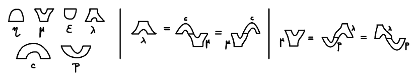
Figure 5. The Frobenius relations.

A graded Frobenius algebra is called commutative and cocommutative if ${\bm{\mu}}$ is commutative and ${\bm{\lambda}}$ is cocommutative. If this is the case and in addition ${\bm{\mu}}$ and ${\bm{\lambda}}$ have opposite parity, then involutivity

$${\bm{\mu}}{\bm{\lambda}}=0$$

holds if $2$ is not a zero-divisor in $R$. In general, a graded Frobenius algebra need not be involutive.

Duality. The dual module $A^{\vee}$ is defined by $(A^{\vee})_{i}=\mathrm{Hom}(A_{-i},R)$. We have a canonical degree $0$ pairing $\langle\cdot,\cdot\rangle:A^{\vee}\otimes A\to R$, $\langle f,a\rangle=f(a)$. Given a graded map $A\stackrel{{\scriptstyle\varphi}}{{\longrightarrow}}B$ we obtain a graded dual map $B^{\vee}\stackrel{{\scriptstyle\varphi^{\vee}}}{{\longrightarrow}}A^{\vee}$. This is defined by $\langle\varphi^{\vee}g,a\rangle=(-1)^{|g||\varphi|}\langle g,\varphi(a)\rangle$.

Given a copairing ${\bm{c}}:R\to A\otimes A$ we denote

$$\vec{\bm{c}}:A^{\vee}\to A$$

the map $\vec{\bm{c}}=(\mathrm{ev}\otimes 1)(1\otimes{\bm{c}})$, i.e. $\vec{\bm{c}}(f)=(-1)^{|f||{\bm{c}}|}(f\otimes 1){\bm{c}}$. Given a pairing ${\bm{p}}:A\otimes A\to R$ we denote

$$\vec{\bm{p}}:A\to A^{\vee}$$

the unique map such that ${\bm{p}}=\mathrm{ev}(\vec{\bm{p}}\otimes 1)$, i.e. $\vec{\bm{p}}(a)(b)={\bm{p}}(a\otimes b)$.

Here we say that a morphism $\varphi:A\to B$ between graded $R$-modules intertwines products ${\bm{\mu}}_{B},{\bm{\mu}}_{B}$ if

$$\varphi{\bm{\mu}}_{A}=(-1)^{|\varphi||{\bm{\mu}}_{A}|}{\bm{\mu}}_{B}\varphi^{\otimes 2}.$$

If this holds and ${\bm{\mu}}_{A}$ is unital with unit ${\bm{\eta}}_{A}$, then ${\bm{\mu}}_{B}$ is unital with unit

$${\bm{\eta}}_{B}=(-1)^{|\varphi|}\varphi{\bm{\eta}}_{A}.$$

We say that $\varphi$ intertwines coproducts ${\bm{\lambda}}_{A},{\bm{\lambda}}_{B}$ if

$$\varphi^{\otimes 2}{\bm{\lambda}}_{A}=(-1)^{|\varphi||{\bm{\lambda}}_{A}|}{\bm{\lambda}}_{B}\varphi.$$

If this holds and ${\bm{\lambda}}_{B}$ is counital with counit ${\bm{{\varepsilon}}}_{B}$, then ${\bm{\lambda}}_{A}$ is counital with counit

$${\bm{{\varepsilon}}}_{A}={\bm{{\varepsilon}}}_{B}\varphi.$$

With this terminology, we have

Theorem 5.4 (Algebraic Poincaré duality [22]).

Let $(A,{\bm{\mu}},{\bm{\lambda}},{\bm{\eta}},{\bm{{\varepsilon}}})$ be a graded Frobenius algebra with pairing ${\bm{p}}$ and copairing ${\bm{c}}$. Then the maps

$$\vec{\bm{p}}:A\to A^{\vee},\qquad\vec{\bm{c}}:A^{\vee}\to A$$

are mutually inverse isomorphisms of graded Frobenius algebras

$$(A,{\bm{\mu}},{\bm{\lambda}},{\bm{\eta}},{\bm{{\varepsilon}}})\simeq(A^{\vee},(-1)^{|{\bm{\lambda}}|}{\bm{\lambda}}^{\vee}\tau,(-1)^{|{\bm{\lambda}}|}\tau{\bm{\mu}}^{\vee},{\bm{{\varepsilon}}}^{\vee},(-1)^{|{\bm{\lambda}}|}{\bm{\eta}}^{\vee}),$$

i.e. they intertwine the products, they intertwine the coproducts, and they preserve the units and counits.

Thus Poincaré duality holds automatically on each Frobenius algebra. The following criterion will be useful.

Proposition 5.5 ([22]).

Let $(A,{\bm{\mu}},{\bm{\lambda}},{\bm{\eta}})$ with ${\bm{c}}={\bm{\lambda}}{\bm{\eta}}$ satisfy the following conditions:

• (unit) the element ${\bm{\eta}}$ is the unit for the degree zero product ${\bm{\mu}}$.

• (associativity) the product ${\bm{\mu}}$ is associative.

• (unital coFrobenius)

  $${\bm{\lambda}}=(1\otimes{\bm{\mu}})({\bm{c}}\otimes 1)=({\bm{\mu}}\otimes 1)(1\otimes{\bm{c}}).$$

• (symmetry)

  $$\tau{\bm{c}}=(-1)^{|{\bm{\lambda}}|}{\bm{c}}.$$

• (isomorphism) the induced map $\vec{\bm{c}}:A^{\vee}\to A$ is an isomorphism.

Then ${\bm{{\varepsilon}}}=(-1)^{|{\bm{\lambda}}|}{\bm{\eta}}^{\vee}\vec{\bm{c}}^{-1}$ makes $(A,{\bm{\mu}},{\bm{\lambda}},{\bm{\eta}},{\bm{{\varepsilon}}})$ a graded Frobenius algebra.

5.2. Product and unit on $SH_{*}({\partial}V)$

To prove Theorems 5.1 and 5.2, we will construct a product ${\bm{\mu}}$ with unit ${\bm{\eta}}$ and a coproduct ${\bm{\lambda}}$ on $SH_{*}({\partial}V)$ and verify the relations in Proposition 5.5.

The product ${\bm{\mu}}$ is induced by the usual pair-of-pants product, and ${\bm{\eta}}$ is induced by the count of spheres with one negative puncture of weight $1$. It is well-known that ${\bm{\mu}}$ is commutative and associative with unit ${\bm{\eta}}$.

5.3. The primary coproduct on $SH_{*}({\partial}V)$ vanishes

We give in this subsection a second proof of the vanishing of the primary coproduct on $SH_{*}({\partial}V)$ from Theorem 4.10. This is useful for the direct definition of the secondary coproduct which we give in §5.4.

Let $H=H_{\lambda,\mu}$ with $\lambda<0<\mu$ as in §4.4 and $a<b$. The genus zero Riemann surface $\Sigma$ with 1 positive puncture, 2 negative punctures, and fixed cylindrical ends at the punctures, together with the choice of a non-positive $1$-form with weights $(1;2,2)$ at the punctures in the sense of §4.2, defines a degree $-n$ primary coproduct

$$\bm{\lambda}^{\text{primary}}:FC_{*}(H)\to FC_{*}(2H)\otimes FC_{*}(2H).$$

Since the sum of Hamiltonian actions at the output is less than or equal to the action at the input, it acts with respect to the action filtrations as

$$\bm{\lambda}^{\text{primary}}:FC_{*}^{\leq a}(H)\to FC_{*}^{\leq\frac{a}{2}}(2H)\otimes FC_{*}(2H)+FC_{*}(2H)\otimes FC_{*}^{\leq\frac{a}{2}}(2H)$$

and

$$\bm{\lambda}^{\text{primary}}:FC_{*}^{<b}(H)\to\bigoplus_{b_{1}+b_{2}=b}FC_{*}^{<b_{1}}(2H)\otimes FC_{*}^{<b_{2}}(2H).$$

Combining these for $a<b$, we get

$$\bm{\lambda}^{\text{primary}}:FC_{*}^{(a,b)}(H)\to\bigoplus_{b_{1}+b_{2}=b}FC_{*}^{(\frac{a}{2},b_{1})}(2H)\otimes FC_{*}^{(\frac{a}{2},b_{2})}(2H).$$

Passing to homology and in the limit over $H$ we obtain the degree $-n$ primary coproduct

$$\bm{\lambda}^{\text{primary}}:SH_{*}^{(a,b)}({\partial}V)\to\bigoplus_{b_{1}+b_{2}=b}SH_{*}^{(\frac{a}{2},b_{1})}({\partial}V)\otimes SH_{*}^{(\frac{a}{2},b_{2})}({\partial}V).$$

Proposition 5.6.

The primary coproduct

$$\bm{\lambda}^{\text{primary}}:SH_{*}^{(a,b)}({\partial}V)\to\bigoplus_{b_{1}+b_{2}=b}SH_{*}^{(\frac{a}{2},b_{1})}({\partial}V)\otimes SH_{*}^{(\frac{a}{2},b_{2})}({\partial}V).$$

vanishes for all $a<b$.

Proof.

Given $H=H_{\lambda,\mu}$ we denote $L=H_{\lambda,\lambda}$. The homology coproduct

$$\bm{\lambda}^{\text{primary}}:FH_{*}^{(a,b)}(H)\to\bigoplus_{b_{1}+b_{2}=b}FH_{*}^{(\frac{a}{2},b_{1})}(2H)\otimes FH_{*}^{(\frac{a}{2},b_{2})}(2H)$$

does not depend on the choice of non-positive $1$-form on the Riemann surface $\Sigma$. In particular, the latter can be chosen as follows: it has weights $(1;-1,2)$ away from a neighborhood of $-\infty$ in the cylindrical end at the first negative puncture, it has weight $-1$ on a long neck in that cylindrical end, and it has weight $2$ at $-\infty$ in that cylindrical end. As such, we obtain a factorization

$$\bm{\lambda}^{\text{primary}}=(c\otimes 1)\bm{\lambda}^{\prime},$$

where at chain level

$$\bm{\lambda}^{\prime}:FC_{*}^{(a,b)}(H)\to\bigoplus_{b_{1}+b_{2}=b}FC_{*}^{(\frac{a}{2},b_{1})}(-H)\otimes FC_{*}^{(\frac{a}{2},b_{2})}(2H)$$

is a primary coproduct and $c:FC_{*}^{(\frac{a}{2},b_{1}}(-H)\to FC_{*}^{(\frac{a}{2},b_{1})}(2H)$ is a continuation map. The point now is that the continuation map $c$ factors as $FC_{*}^{(\frac{a}{2},b_{1})}(-H)\to FC_{*}^{(\frac{a}{2},b_{1})}(L)\to FH_{*}^{(\frac{a}{2},b_{1})}(2H)$. Since $FC_{*}^{(\frac{a}{2},b_{1})}(L)=0$ for $\lambda<a$, we obtain $c=0$ in this range. Passing to homology and the limit over $H=H_{\lambda,\mu}$ as $\lambda\to-\infty$ and $\mu\to\infty$ thus yields the desired vanishing result. ∎

5.4. Secondary coproduct on $SH_{*}({\partial}V)$

We give in this subsection a direct definition of the degree $-n+1$ secondary coproduct $\bm{\lambda}$ on $SH_{*}({\partial}V)$. It follows from [23] that this is dual to the degree $n-1$ secondary product on Rabinowitz Floer cohomology from Theorem 4.8.

The vanishing of $\bm{\lambda}^{\text{primary}}$ was proved above by factoring out a continuation map at the first negative puncture. The same argument could have been carried at the second negative puncture. The secondary coproduct $\bm{\lambda}$ is obtained by interpolating between these two constructions.

Consider again the genus $0$ Riemann surface $\Sigma$ with 1 positive puncture, 2 negative punctures and fixed cylindrical ends at the punctures, with coordinates $z=s+it$, $t\in S^{1}$, $s\in(-\infty,0]$ at the negative punctures. We pick a smooth $1$-parameter family of Floer data $H_{\tau},\beta_{\tau}$, $\tau\in(0,1)$, on $\Sigma$ as follows (see Figure 6).

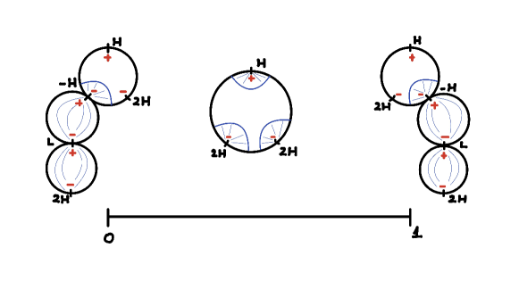
Figure 6. Definition of the coproduct with broken homotopies at the endpoints.

Outside the negative cylindrical ends $H_{\tau}=H$ as in the previous subsection, and the $1$-forms $\beta_{\tau}\in\Omega^{1}(\Sigma)$ satisfy $d\beta_{\tau}=0$ and are equal to $dt$ on the positive cylindrical end, and to $f(\tau)dt$ resp. $(1-f(\tau))dt$ near the negative boundaries. Here $f:[0,1]\to[-1,2]$ is a smooth function which equals $-1$ on $[0,\delta]$ and $2$ on $[1-\delta,1]$, for some $\delta>0$.

On the first negative cylindrical end $(-\infty,0]\times S^{1}$ we write $H_{\tau}\beta_{\tau}=H_{\tau,s}dt$ for a family $H_{\tau,s}$ of $s$-dependent Hamiltonians with $\frac{{\partial}H_{\tau,s}}{{\partial}s}\leq 0$ and the following properties:

• $H_{\tau,s}$ is equal to $f(\tau)H$ near $s=0$, and to $2H$ for $s\leq-R(\tau)$;

• $H_{\tau,s}=L$ for $\tau\in[0,\delta]$ and $s\in[-R(\tau)+1,-1]$.

Here $R:(0,1]\to[0,\infty)$ is a nonincreasing smooth function with $R(1)=0$, $R(\delta)=3$, and $\lim_{\tau\to 0}R(\tau)=\infty$.

On the second negative cylindrical end $(-\infty,0]\times S^{1}$ we write $H_{\tau}\beta_{\tau}=H_{\tau,s}dt$ for a family $H_{\tau,s}$ of $s$-dependent Hamiltonians with $\frac{{\partial}H_{\tau,s}}{{\partial}s}\leq 0$ and the following properties:

• $H_{\tau,s}$ is equal to $(1-f(\tau))H$ near $s=0$, and to $2H$ for $s\leq-R(1-\tau)$;

• $H_{\tau,s}=L$ for $\tau\in[1-\delta,1]$ and $s\in[-R(1-\tau)+1,-1]$.

Note that at $\tau=0$ the Riemann surface $\Sigma$ degenerates into a nodal Riemann surface consisting of a 3-punctured sphere with asymptotics $(H;-H,2H)$, and a chain of two cylinders with asymptotics $(-H;L)$ and $(L;2H)$ attached at the first negative puncture. A similar degeneration occurs at $\tau=1$ at the second negative puncture, see Figure 6.

By construction, the Floer data $H_{\tau}\beta_{\tau}$ satisfy conditions (i) and (ii) in §4.2. So the moduli spaces of pairs $(\tau,u)$, with $\tau\in[0,1]$ and $u:\Sigma\to\widehat{V}$ solving $(du-X_{H_{\tau}}\otimes d\beta_{\tau})^{0,1}=0$ with given asymptotics, are compact up to Floer breaking. The signed count of $0$-dimensional such moduli spaces therefore defines a degree $-n+1$ map

$$\bm{\lambda}:FC_{*}(H)\to FC_{*}(2H)^{\otimes 2},$$

where the $+1$ in the degree comes from the parameter $\tau$. As in the case of $\bm{\lambda}^{\text{primary}}$, for $a<b$ action considerations yield

$$\bm{\lambda}:FC_{*}^{(a,b)}(H)\to\bigoplus_{b_{1}+b_{2}=b}FC_{*}^{(\frac{a}{2},b_{1})}(2H)\otimes FC_{*}^{(\frac{a}{2},b_{2})}(2H).$$

Again, the key point now is that for fixed parameters $a<b$ we have $FC_{*}^{(\frac{a}{2},b)}(L)=0$ if the slope of $L$ satisfies $\lambda<a$. Since the contributions to ${\bm{\lambda}}$ at $\tau=0,1$ factor through $FC_{*}^{(\frac{a}{2},b)}(L)$, this implies that ${\bm{\lambda}}$ is a chain map. Passing to homology and in the limit over $H$ we obtain

$$\bm{\lambda}:SH_{*}^{(a,b)}({\partial}V)\to\bigoplus_{b_{1}+b_{2}=b}SH_{*}^{(\frac{a}{2},b_{1})}({\partial}V)\otimes SH_{*}^{(\frac{a}{2},b_{2})}({\partial}V).$$

Passing to the inverse limit over $a\to-\infty$ and then to the direct limit over $b\to\infty$ we obtain the degree $-n+1$ secondary coproduct

$$\bm{\lambda}:SH_{*}({\partial}V)\to SH_{*}({\partial}V)\,\widehat{\otimes}\,SH_{*}({\partial}V),$$

where the completed tensor product on the right hand side is defined by

$$SH_{*}({\partial}V)\,\widehat{\otimes}\,SH_{*}({\partial}V):=\lim^{\longrightarrow}_{b\to\infty}\lim^{\longleftarrow}_{a\to-\infty}\bigoplus_{b_{1}+b_{2}=b}SH_{*}^{(\frac{a}{2},b_{1})}({\partial}V)\otimes SH_{*}^{(\frac{a}{2},b_{2})}({\partial}V).$$

Standard arguments show that this coproduct is canonical, i.e. it does not depend on the various choices involved in the construction. It follows directly from the definition that ${\bm{\lambda}}$ is cocommutative on $S{\mathbb{H}}_{*}({\partial}V)$.

Remark 5.7 (Completed tensor product).

By construction, $SH_{k}({\partial}V)$ carries an increasing filtration by the subspaces

$$SH^{<b}_{k}({\partial}V)=\lim\limits^{\longleftarrow}_{a\to-\infty}SH_{k}^{(a,b)}({\partial}V)$$

satisfying

$$SH^{<b}_{k}({\partial}V)\subset SH^{<b^{\prime}}_{k}({\partial}V)\text{ for }b<b^{\prime},\qquad\bigcup_{b\in{\mathbb{R}}}SH^{<b}_{k}({\partial}V)=SH_{k}({\partial}V).$$

For $x\in SH_{k}({\partial}V)$ set

$$\|x\|:=\inf\{b\in{\mathbb{R}}\mid x\in SH_{k}^{<b}({\partial}V)\}.$$

Consider now a formal sum $\sum_{i=0}^{\infty}x_{i}\otimes x_{i}^{\prime}$ with $x_{i},x_{i}^{\prime}\in SH_{*}({\partial}V)$ satisfying $\mathrm{CZ}(x_{i})+\mathrm{CZ}(x_{i}^{\prime})=k$ and

$$\lim_{i\to\infty}\min\{\|x_{i}\|,\|x_{i}^{\prime}\|\}=-\infty,\qquad\sup_{i}(\|x_{i}\|+\|x_{i}^{\prime}\|))<\infty.$$

Then this sum canonically defines an element of $SH_{*}({\partial}V)\,\widehat{\otimes}\,SH_{*}({\partial}V)$ in degree $k$.

5.5. The unital coFrobenius relation

Let ${\bm{\mu}},{\bm{\lambda}},{\bm{\eta}}$ be the operations on $S{\mathbb{H}}_{*}({\partial}V)$ constructed in the preceding subsections and define ${\bm{c}}={\bm{\lambda}}{\bm{\eta}}.$ A standard neck-stretching argument shows that ${\bm{c}}$ is induced by counting configurations as in Figure 6 without the positive puncture. This directly implies the (symmetry) $\tau{\bm{c}}=(-1)^{|{\bm{\lambda}}|}{\bm{c}}$.

Proposition 5.8.

The operations ${\bm{\mu}}$ and ${\bm{c}}$ on $S{\mathbb{H}}_{*}({\partial}V)$ satisfy the (unital coFrobenius) relation

$${\bm{\lambda}}=(1\otimes{\bm{\mu}})({\bm{c}}\otimes 1)=({\bm{\mu}}\otimes 1)(1\otimes{\bm{c}}).$$

Proof.

For $\lambda<0<\mu$ recall the Hamiltonians $H=H_{\lambda,\mu}$ and $L=L_{\lambda}$ from above, and consider the new Hamiltonians $S$ and $T$ in Figure 7. Recalling the notation $V_{\delta}$, $\delta>0$ from the beginning of the proof of Theorem 4.8, their explicit description is the following: the Hamiltonian $S$ is constant equal to $\lambda/2$ on $V_{\frac{1}{2}}$, it is linear of slope $-\lambda$ on $V\setminus V_{\frac{1}{2}}$, and it is linear of slope $2\mu$ outside of $V$; the Hamiltonian $T$ is constant equal to $\lambda$ on $V_{\frac{1}{2}}$, it is linear of slope $2\lambda$ on $V\setminus V_{\frac{1}{2}}$, and it is linear of slope $-\mu$ outside $V$.

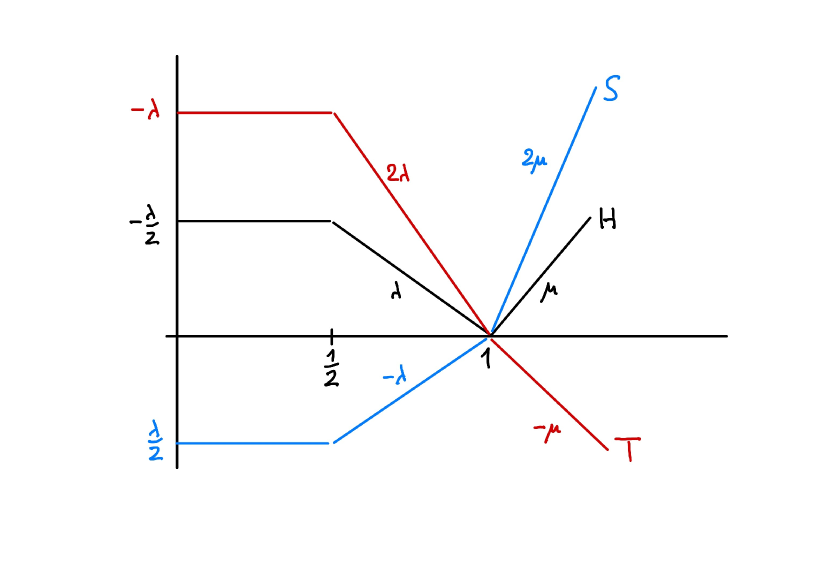
Figure 7. The Hamiltonians $S$ and $T$.

They have the following properties:

1. $H=S+T$ and $-H\leq S,T\leq 2H$.

2. The count of Floer spheres with one positive puncture at $H$ and two negative punctures at $S$ and $T$ is well-defined.

3. For fixed $-\infty<a<b<\infty$ and $\mu,-\lambda$ sufficiently large, $S$ and $T$ have no $1$-periodic orbits with action in $[a,b]$; the same holds for $(1-\tau)S-\tau L$ and $(1-\tau)T+\tau L$ with $\tau\in[0,1]$.

Consider now the moduli space of punctured Floer spheres shown in Figure 8.

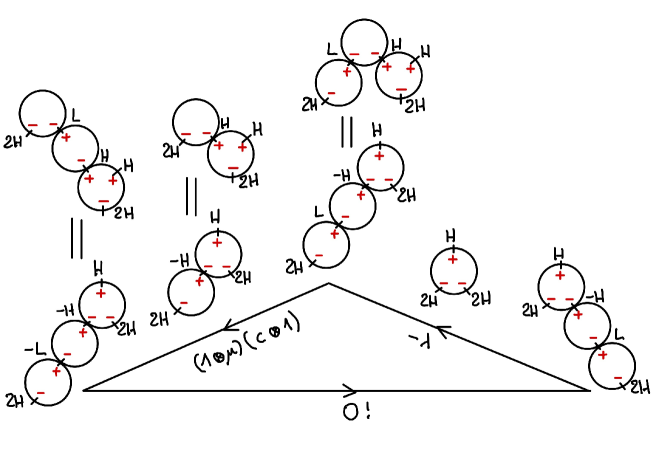
Figure 8. Proof of the unital coFrobenius relation.

Here the upper right side describes $-{\bm{\lambda}}$ and the upper left side the composition $(1\otimes{\bm{\mu}})({\bm{c}}\otimes 1)$. The lower side is described in Figure 9.

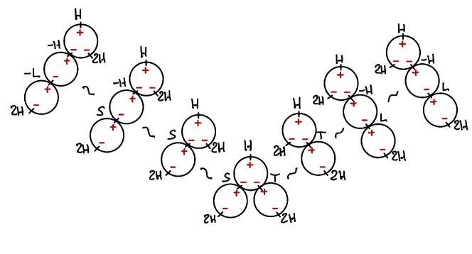
Figure 9. Vanishing of the lower side.

Here (going from left to right) the first deformation linearly interpolates between $-L$ and $S$, the second one glues the puncture at $-H$, the third one splits off the puncture at $T$, the fourth one glues the puncture at $S$, the fifth one splits off the puncture at $-H$, and the sixth one linearly interpolates between $T$ and $L$. In view of properties (1) and (2) above all the corresponding counts are well-defined. For a finite action window $(a,b)$ and $\mu,-\lambda$ sufficiently large, all these counts vanish by property (3) because we always have at least one puncture at $S$, $T$, $(1-\tau)S-\tau L$, or $(1-\tau)T+\tau L$ with $\tau\in[0,1]$. We extend the configurations over the interior of the triangle in Figure 8 by linear interpolation. This proves the first equality of the (unital coFrobenius) relation in a fixed finite action window, and by taking inverse and direct limits it follows on $S{\mathbb{H}}_{*}({\partial}V)$.

The second equality can be proved analogously. Alternatively, it can be formally deduced from the first one by verifying the identity

$$\tau{\bm{\lambda}}=({\bm{\mu}}\tau\otimes 1)(1\otimes\tau{\bm{c}}).$$

and applying the symmetries

$$\tau{\bm{\lambda}}=(-1)^{|{\bm{\lambda}}|}{\bm{\lambda}},\qquad\tau{\bm{c}}=(-1)^{|{\bm{\lambda}}|}{\bm{c}},\qquad{\bm{\mu}}\tau=(-1)^{|{\bm{\mu}}|}{\bm{\mu}}.$$

∎

5.6. The copairing is the inverse of the Poincaré duality isomorphism

Let ${\bm{c}}={\bm{\lambda}}{\bm{\eta}}$ be as in the preceding subsection and recall the notation $\vec{\bm{c}}=(\mathrm{ev}\otimes 1)(1\otimes{\bm{c}})$. We shall sometimes refer to $\vec{\bm{c}}$ as being the secondary continuation map. See [24] for a related discussion.

Proposition 5.9.

The map $-\vec{\bm{c}}:SH^{1-*}({\partial}V)\to SH_{*}({\partial}V)$ is the inverse of the Poincaré duality isomorphism in Theorem 4.8.

Proof.

Let $H=H_{\lambda,\mu}$ be a V-shaped Hamiltonian as in Figure 3 and $L=H_{\lambda,\lambda}$ the corresponding linear Hamiltonian. By construction, the map $\vec{\bm{c}}$ counts cylinders in the $1$-parametric moduli space shown in Figure 10.

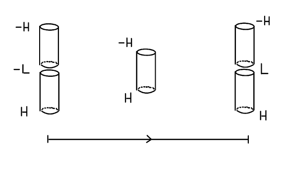
Figure 10. The map $\vec{\bm{c}}$.

As in the proof of Theorem 4.8, we fix a finite action window $(a,b)$ and consider for $\tau\gg 0$ the dented Hamiltonian in Figure 4, redrawn in Figure 11. Let us denote this Hamiltonian by $Z$. Recall that its Floer chain complex in the action window $(a,b)$ has the form

$$FC^{(a,b)}(Z)=C^{-}\oplus C^{+},\qquad{\partial}_{Z}=\begin{pmatrix}{\partial}^{-}&f\\ 0&{\partial}^{+}\end{pmatrix},$$

where $C^{-}$ and $C^{+}$ are generated by orbit groups III and II, respectively, and $f:C^{+}\to C^{-}$ is a map of degree $-1$.

Let $K$ be the Hamiltonian which agrees with $Z$ to the left of orbit group III and with $H$ to its right, see Figure 11.

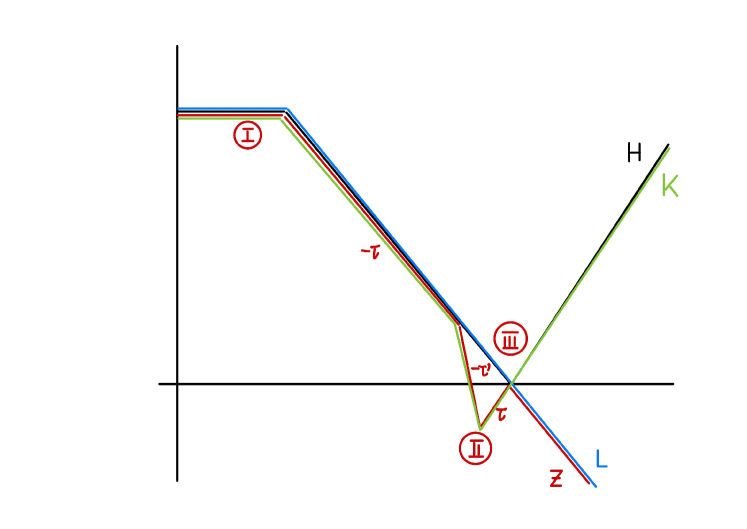
Figure 11. The Hamiltonians $H,L,Z,K$.

Monotone homotopies $Z\leadsto L\leadsto H$ and $Z\leadsto K\leadsto H$ give rise to a diagram of chain maps

which commutes up to a degree $1$ chain homotopy

$$\Phi:\bigl{(}FC^{(a,b)}(Z),{\partial}_{Z}\bigr{)}\to\bigl{(}FC^{(a,b)}(H),{\partial}_{H}\bigr{)}.$$

This means that

$${\partial}_{H}\Phi+\Phi{\partial}_{Z}=F_{1}-F_{0}$$

for the compositions

$$F_{0}:FC^{(a,b)}(Z)\to FC^{(a,b)}(L)\to FC^{(a,b)}(H),$$

$$F_{1}:FC^{(a,b)}(Z)\to FC^{(a,b)}(K)\to FC^{(a,b)}(H).$$

Writing $\Phi=(\Phi^{-},\Phi^{+})$ and $F_{i}=(F_{i}^{-},F_{i}^{+})$ with respect to the splitting $FC^{(a,b)}(Z)=C^{-}\oplus C^{+}$, the relation reads

$$\left\{\begin{aligned} {\partial}_{H}\Phi^{+}+\Phi^{+}{\partial}^{+}+\Phi^{-}f&=F_{1}^{+}-F_{0}^{+},\cr{\partial}_{H}\Phi^{-}+\Phi^{-}{\partial}^{-}&=F_{1}^{-}-F_{0}^{-}.\end{aligned}\right.$$

Now observe that $F_{0}^{\pm}=0$ because the map $F_{0}$ factors through $FC^{(a,b)}(L)=\{0\}$, and the map

$$F_{1}^{+}:C^{+}\stackrel{{\scriptstyle\cong}}{{\longrightarrow}}FC^{(a,b)}(K)\stackrel{{\scriptstyle\cong}}{{\longrightarrow}}FC^{(a,b)}(H)$$

is the identity under the canonical identifications of the chain complexes. Hence the first relation above becomes ${\partial}_{H}\Phi^{+}+\Phi^{+}{\partial}^{+}+\Phi^{-}f=1$, so on homology the composition in the upper row of

is the identity. Commutativity of the first square follows from the definition of the Poincaré duality isomorphism in the proof of Theorem 4.8. The second square commutes because the map $\Phi^{-}:C^{-}\to FC^{(a,b)}(H)$ interpolates between the factorizations through $FC^{(a,b)}(L)$ and $FC^{(a,b)}(K)$, which agrees with the definition of the secondary continuation map $-\vec{\bm{c}}$ (see Figure 10). This proves $(-\vec{\bm{c}})\circ PD=1$ on $SH_{*}^{(a,b)}({\partial}V)$. In the inverse-direct limit we obtain that $(-\vec{\bm{c}})\circ PD=1$ on $SH_{*}({\partial}V)$, i.e. $-\vec{\bm{c}}$ is the inverse of the isomorphism $PD$. ∎

5.7. Proof of Theorems 5.1 and 5.2

Proof of Theorem 5.1.

By §5.2, the degree $0$ product ${\bm{\mu}}$ on $S{\mathbb{H}}_{*}({\partial}V)$ is commutative and associative with unit ${\bm{\eta}}$. The degree $1-2n$ coproduct ${\bm{\lambda}}$ is defined in §5.4. By construction, ${\bm{\lambda}}$ is cocommutative and the associated copairing ${\bm{c}}={\bm{\lambda}}{\bm{\eta}}$ is symmetric. By Proposition 5.8 the (unital coFrobenius) relation holds, and by Proposition 5.9 the map $-\vec{\bm{c}}:S{\mathbb{H}}^{1-2n-*}({\partial}V)\to S{\mathbb{H}}_{*}({\partial}V)$ is the inverse of the Poincaré duality isomorphism. Thus $({\bm{\mu}},{\bm{\lambda}},{\bm{\eta}})$ satisfies the conditions in Proposition 5.5 and it follows that ${\bm{{\varepsilon}}}=-{\bm{\eta}}^{\vee}\vec{\bm{c}}^{-1}$ makes $(S{\mathbb{H}}_{*}({\partial}V),{\bm{\mu}},{\bm{\lambda}},{\bm{\eta}},{\bm{{\varepsilon}}})$ a graded Frobenius algebra. Finally, it follows from Theorem 5.4 that $-\vec{\bm{c}}$ and its inverse $-\vec{\bm{p}}=PD$ intertwine the graded Frobenius algebra structures on $S{\mathbb{H}}_{*}({\partial}V)$ and $S{\mathbb{H}}^{-*}({\partial}V)$. ∎

Proof of Theorem 5.2.

The proof is up to notation the same as that of Theorem 5.1, using the gradings in Appendix A. Note that commutativity of ${\bm{\mu}}$ and cocommutativity of ${\bm{\lambda}}$ need not hold in this case, but symmetry of ${\bm{c}}$ is still satisfied because ${\bm{c}}$ is counting disks with only two boundary punctures. ∎

6. Graded open-closed TQFT structure

In this section we show that the graded Frobenius algebra structure on V-shaped symplectic homology and its Lagrangian counterpart from §5 fit together to a graded version of a two-dimensional open-closed TQFT.

6.1. Two-dimensional open-closed TQFTs

We begin by recalling the description of a two-dimensional open-closed TQFT in terms of generators and relations from Lauda and Pfeiffer [51]. It associates to the circle a finite dimensional free $R$-module $C$ and to the closed interval a finite dimensional free $R$-module $A$. Its generators are the following operations (see Figure 12):

• the product ${\bm{\mu}}_{C}:C\otimes C\to C$ and the unit ${\bm{\eta}}_{C}:R\to C$;

• the coproduct ${\bm{\lambda}}_{C}:C\to C\otimes C$ and the counit ${\bm{{\varepsilon}}}_{C}:C\to R$;

• the product ${\bm{\mu}}_{A}:A\otimes A\to A$ and the unit ${\bm{\eta}}_{A}:R\to A$;

• the coproduct ${\bm{\lambda}}_{A}:A\to A\otimes A$ and the counit ${\bm{{\varepsilon}}}_{A}:A\to R$;

• the zipper (or closed-open map) ${\bm{\zeta}}:C\to A$;

• the cozipper (or open-closed map) ${\bm{\zeta}}^{*}:A\to C$.

These satisfy the following relations (in our terminology):

1. $(C,{\bm{\mu}}_{C},{\bm{\eta}}_{C},{\bm{\lambda}}_{C},{\bm{{\varepsilon}}}_{C})$ is a commutative and cocommutative Frobenius algebra.

2. $(A,{\bm{\mu}}_{A},{\bm{\eta}}_{A},{\bm{\lambda}}_{A},{\bm{{\varepsilon}}}_{A})$ is a Frobenius algebra.

3. The zipper is an algebra homomorphism,

   $${\bm{\mu}}_{A}({\bm{\zeta}}\otimes{\bm{\zeta}})={\bm{\zeta}}\,{\bm{\mu}}_{C},\qquad{\bm{\zeta}}\,{\bm{\eta}}_{C}={\bm{\eta}}_{A}.$$

4. The zipper lands in the center of ${\bm{\mu}}_{A}$,

   $${\bm{\mu}}_{A}({\bm{\zeta}}\otimes 1)={\bm{\mu}}_{A}\tau({\bm{\zeta}}\otimes 1).$$

5. The cozipper is dual to the zipper via the copairings ${\bm{c}}_{C}={\bm{\lambda}}_{C}{\bm{\eta}}_{C}$ and ${\bm{c}}_{A}={\bm{\lambda}}_{A}{\bm{\eta}}_{A}$,

   $$(1\otimes{\bm{\zeta}}){\bm{c}}_{C}=({\bm{\zeta}}^{*}\otimes 1){\bm{c}}_{A}.$$

6. The Cardy condition

   $${\bm{\zeta}}\,{\bm{\zeta}}^{*}={\bm{\mu}}_{A}\tau{\bm{\lambda}}_{A}.$$

In [51] condition (5) is stated as the equivalent condition in Lemma 6.2 below (without signs), and it is proved that a 2D open-closed TQFT is equivalent to the algebraic structure defined by these generators and relations.

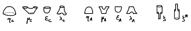
Figure 12. The generators of an open-closed TQFT.

6.2. Graded open-closed TQFTs

In this subsection we adapt the description of a two-dimensional open-closed TQFT to the graded setting, also dropping the finite dimensionality conditions on $C$ and $A$. Thus $C$ and $A$ are now ${\mathbb{Z}}$-graded free $R$-modules. We either assume that $C$ and $A$ are of finite type, i.e. finite dimensional in each degree, or they are endowed with additional filtrations as in Remark 5.7, and it is understood that ${\bm{\lambda}}_{C}$ and ${\bm{\lambda}}_{A}$ take values in completed tensor products. See also [22, §8].

After shifting degrees, we can and will assume that the products ${\bm{\mu}}_{C}$ and ${\bm{\mu}}_{A}$ have degree $0$. Then relations (1)–(5) determine all the other degrees in terms of the degrees of ${\bm{\lambda}}_{C}$ and ${\bm{\lambda}}_{A}$:

$$|{\bm{\mu}}_{C}|=|{\bm{\eta}}_{C}|=|{\bm{\mu}}_{A}|=|{\bm{\eta}}_{A}|=|{\bm{\zeta}}|=0,$$

$$|{\bm{\lambda}}_{C}|=|{\bm{c}}_{C}|=-|{\bm{{\varepsilon}}}_{C}|,\qquad|{\bm{\lambda}}_{A}|=|{\bm{c}}_{A}|=-|{\bm{{\varepsilon}}}_{A}|,$$

$$|{\bm{\zeta}}^{*}|=|{\bm{\lambda}}_{C}|-|{\bm{\lambda}}_{A}|.$$

Relation (6) yields the additional condition $|{\bm{\zeta}}^{*}|=|{\bm{\lambda}}_{A}|$, which combined with the previous one implies that $|{\bm{\lambda}}_{C}|=2|{\bm{\lambda}}_{A}|$ is even. This gives rise to an algebraic structure which recovers the one of the previous subsection in the case that $|{\bm{\lambda}}_{A}|$ is also even.

On degree shifted symplectic homology $S{\mathbb{H}}_{*}({\partial}V)$, however, the coproduct ${\bm{\lambda}}_{C}$ has odd degree $1-2n$, so the associated open-closed structure cannot satisfy the Cardy condition. This leads us to the following definition.

Definition 6.1 (cf. [22, Definition 6.1]).

A graded (two-dimensional) open-closed TQFT consists of two ${\mathbb{Z}}$-graded free $R$-modules $C,A$ and operations as above satisfying the following signed versions of relations (1)–(5) above:

1. $(C,{\bm{\mu}}_{C},{\bm{\eta}}_{C},{\bm{\lambda}}_{C},{\bm{{\varepsilon}}}_{C})$ is a commutative and cocommutative graded Frobenius algebra, called the closed sector.

2. $(A,{\bm{\mu}}_{A},{\bm{\eta}}_{A},{\bm{\lambda}}_{A},{\bm{{\varepsilon}}}_{A})$ is a graded Frobenius algebra, called the open sector.

3. The zipper is an algebra homomorphism,

   $${\bm{\mu}}_{A}({\bm{\zeta}}\otimes{\bm{\zeta}})={\bm{\zeta}}\,{\bm{\mu}}_{C},\qquad{\bm{\zeta}}\,{\bm{\eta}}_{C}={\bm{\eta}}_{A}.$$

4. The zipper lands in the center of ${\bm{\mu}}_{A}$,

   $${\bm{\mu}}_{A}({\bm{\zeta}}\otimes 1)={\bm{\mu}}_{A}\tau({\bm{\zeta}}\otimes 1).$$

5. The cozipper is dual to the zipper via the copairings ${\bm{c}}_{C}={\bm{\lambda}}_{C}{\bm{\eta}}_{C}$ and ${\bm{c}}_{A}={\bm{\lambda}}_{A}{\bm{\eta}}_{A}$,

   $$(1\otimes{\bm{\zeta}}){\bm{c}}_{C}=({\bm{\zeta}}^{*}\otimes 1){\bm{c}}_{A}.$$

6. The graded Cardy condition

   $${\bm{\zeta}}\,{\bm{\zeta}}^{*}=\begin{cases}(-1)^{|\lambda_{A}|}{\bm{\mu}}_{A}\tau{\bm{\lambda}}_{A}&\text{if }|{\bm{\lambda}}_{C}|=2|{\bm{\lambda}}_{A}|,\cr 0&\text{otherwise}.\end{cases}$$

Lemma 6.2 ([22, Lemma 6.3]).

Assuming relations (1) and (2), relation (5) is equivalent to the following relation in terms of the pairings ${\bm{p}}_{C}=-{\bm{{\varepsilon}}}_{C}{\bm{\mu}}_{C}$ and ${\bm{p}}_{A}=(-1)^{|{\bm{\lambda}}_{A}|}{\bm{{\varepsilon}}}_{A}{\bm{\mu}}_{A}$:

$${\bm{p}}_{C}(1\otimes{\bm{\zeta}}^{*})=(-1)^{|{\bm{\lambda}}_{A}|+1}{\bm{p}}_{A}({\bm{\zeta}}\otimes 1).$$

Consider now a Liouville domain $V$ of dimension $2n$ and an exact Lagrangian submanifold $L\subset V$ with Legendrian boundary ${\partial}L\subset{\partial}V$. We define the zipper (or closed-open map) and cozipper (or open-closed map)

$${\bm{\zeta}}:S{\mathbb{H}}_{*}({\partial}V)\to S{\mathbb{H}}_{*}({\partial}L),\qquad{\bm{\zeta}}^{*}:S{\mathbb{H}}_{*}({\partial}L)\to S{\mathbb{H}}_{*-n}({\partial}V)$$

by counts of discs with one positive interior puncture and one negative boundary puncture, respectively one positive boundary puncture and one negative interior puncture, as shown in Figure 13.

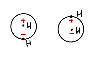
Figure 13. The zipper and cozipper in symplectic homology.

Theorem 6.3 (Graded open-closed TQFT structure on symplectic homology).

Let $V$ be a Liouville domain of dimension $2n$ and $L\subset V$ an exact Lagrangian submanifold with Legendrian boundary ${\partial}L\subset{\partial}V$. Then the graded Frobenius algebra structures on $S{\mathbb{H}}_{*}({\partial}V)$ and $S{\mathbb{H}}_{*}({\partial}L)$, together with the maps ${\bm{\zeta}}$ and ${\bm{\zeta}}^{*}$, fit together into a graded open-closed TQFT structure, with coproducts of degrees $|{\bm{\lambda}}_{C}|=1-2n$ and $|{\bm{\lambda}}_{A}|=1-n$. The Poincaré duality isomorphisms intertwine this structure with the corresponding structure on cohomology $S{{\mathbb{H}}}^{1-2n-*}({\partial}V)$ and $S{{\mathbb{H}}}^{1-n-*}({\partial}L)$.

Proof.

Relations (1) and (2) are Theorems 5.1 and 5.2, respectively. The proofs of relations (3), (4) and (6) are shown in Figures 14, 15 and 16, respectively. Note that here the degrees are such that (6) reads ${\bm{\zeta}}\,{\bm{\zeta}}^{*}=0$.

Figure 14. The zipper is an algebra homomorphism.

Figure 15. The zipper lands in the center.

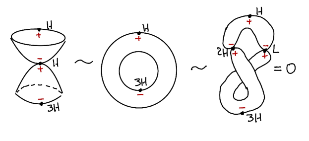
Figure 16. The graded Cardy condition.

The proof of relation (5) is shown in Figure 17. There we consider a moduli space parametrized by a hexagon, where the left side corresponds to $({\bm{\zeta}}^{*}\otimes 1){\bm{c}}_{A}$ and the right side to $-(1\otimes{\bm{\zeta}}){\bm{c}}_{C}$. The operations on the other four sides factor through the Hamiltonian $L$ and therefore vanish because $L$ has no periodic orbits in a given finite action window.

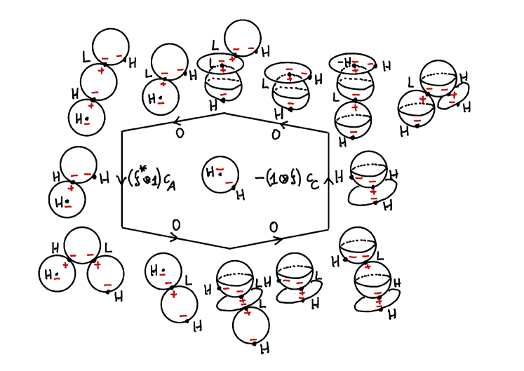
Figure 17. The cozipper is dual to the zipper.

∎

6.3. Topological open-closed and closed-open maps

Now we specialize to the pair $(V,L)=(D^{*}M,D^{*}_{q}M)$, so that we work with Rabinowitz loop homology $\widehat{{\mathbb{H}}}_{*}\Lambda=S{\mathbb{H}}_{*}(S^{*}M)$ and Rabinowitz based loop homology $\widehat{H}_{*}\Omega=S{\mathbb{H}}_{*}(S^{*}_{q}M)$. In this subsection we identify the closed-open and open-closed maps ${\bm{\zeta}},{\bm{\zeta}}^{*}$ described above with their topological counterparts, the topological shriek and pullback/pushforward maps induced by the inclusion $i:{\Omega}\hookrightarrow\Lambda$, denoted $i_{!}$, $i^{*}$ etc. Note that the latter are also well-defined at the level of reduced (co)homology groups.

Proposition 6.4.

With respect to the splittings for $\widehat{H}_{*}\Lambda$ and $\widehat{H}_{*}\Omega$ in Theorem 1.5, the following hold:

(a) The zipper ${\bm{\zeta}}:\widehat{H}_{*}\Lambda\to\widehat{H}_{*-n}\Omega$ restricts to maps $\overline{H}_{*}\Lambda\to H_{*-n}\Omega$ and $\overline{H}^{-*+1}(\Lambda)\to H^{-*+1}\Omega$ which coincide respectively with the topological shriek map $i_{!}$ and the cohomological pullback map $i^{*}$.

(b) The cozipper ${\bm{\zeta}}^{*}:\widehat{H}_{*}\Omega\to\widehat{H}_{*}\Lambda$ restricts to maps $H_{*}\Omega\to\overline{H}_{*}\Lambda$ and $H^{-*+1-n}\Omega\to\overline{H}^{-*+1}\Lambda$ which coincide respectively with the topological pushforward map $i_{*}$ and the cohomological shriek map $i^{!}$.

Proof of Proposition 6.4.

We prove only assertion (a), the proof of (b) being similar. The topological shriek map $i_{!}:H_{*}(\Lambda)\to H_{*-n}(\Omega)$ descends to $i_{!}:\overline{H}_{*}(\Lambda)\to H_{*-n}(\Omega)$ because the point class lies in its kernel for degree reasons. It admits the following description in Morse theory (see [4, 19]). Consider a smooth Lagrange function $L:S^{1}\times TM\to{\mathbb{R}}$ which outside a compact set has the form $L(t,q,v)=\frac{1}{2}|v|^{2}-V_{\infty}(t,q)$ for a smooth potential $V_{\infty}:S^{1}\times M\to{\mathbb{R}}$. It induces a smooth action

$$S_{L}:\Lambda\to{\mathbb{R}},\qquad q\mapsto\int_{0}^{1}L(t,q,\dot{q})dt,$$

which we can assume to be a Morse function whose negative flow with respect to the $W^{1,2}$-gradient $\nabla S_{L}$ is Morse–Smale.

View $\Omega\subset\Lambda$ as a codimension $n$ Hilbert submanifold and choose the base point $q$ generic so that all critical points of $S_{L}$ lie outside $\Omega$. Given $a\in\mathrm{Crit}(S_{L})$ and $b\in\mathrm{Crit}(S_{L}|_{\Omega})$ set

$$\mathcal{M}(a;b):=W^{-}(a)\cap W^{+}(b),$$

where $W^{-}(a)$ is the unstable manifold of $a$ with respect to the flow of $-\nabla S_{L}$ on $\Lambda$, and $W^{+}(b)$ is the stable manifold of $b$ with respect to the flow of $-\nabla(S_{L}|_{\Omega})$ on ${\Omega}$. Generically, this is a manifold of dimension $\dim\mathcal{M}(a,b)=\mathrm{ind}(a)-\mathrm{ind}(b)-n$, where $\mathrm{ind}(a)$ and $\mathrm{ind}(b)$ denote the Morse indices of $a$ and $b$ with respect to $S_{L}$ and $S_{L}|_{\Omega}$, respectively. If its dimension is zero this manifold is compact and defines the map $i_{!}$.

The zipper ${\bm{\zeta}}:\overline{H}_{*}\Lambda\to H_{*-n}\Omega$ can alternatively be described using the usual Hamiltonian profile for the symplectic homology $SH_{*}(T^{*}M)$, i.e. a Hamiltonian that is constant equal to zero on $D^{*}M$ and linear of positive slope with respect to the radial coordinate outside $D^{*}M$.

We use the isomorphism $\Psi_{\Lambda}:SH_{*}(D^{*}M)\stackrel{{\scriptstyle\simeq}}{{\longrightarrow}}H_{*}\Lambda$ from [4, 8]. It is given by a count of mixed configurations consisting of a disc with boundary on the zero section and one positive interior puncture, solving a perturbed Cauchy-Riemann equation, together with a semi-infinite descending gradient line in $\Lambda$ starting at the loop determined by the restriction of the disc to its boundary.

We also use the isomorphism $\Psi_{\Omega}:SH_{*}(D^{*}_{q}M)\stackrel{{\scriptstyle\simeq}}{{\longrightarrow}}H_{*-n}\Omega$ with $\Omega=\Omega_{q}M$, i.e., the Lagrangian counterpart of $\Psi_{\Lambda}$ defined in [4, 8]. It is given by a count of mixed configurations consisting of a disc with three boundary punctures, with one boundary component constrained to $M$, the other two boundary components constrained to $T^{*}_{q}M$, a positive puncture at the end bordered by the two $T^{*}_{q}M$-components, solving a perturbed Cauchy-Riemann equation, together with a semi-infinite descending gradient line in $\Omega$ starting at the loop determined by the restriction of the strip to the boundary component which is constrained to $M$. Note that the strip must be asymptotic to $q$ at each of the punctures bordered by $M$ and $T^{*}_{q}M$, since $q$ is the unique intersection point of $M$ and $T^{*}_{q}M$. Recall that in $H_{*}\Lambda$ and $H_{*-n}\Omega$ we use twisted coefficients as described in Appendix A.2.

We need to show that the following diagram commutes:

We prove that both compositions are equal to the map $\Gamma:SH_{*}(D^{*}M)\break\to H_{*-n}\Omega$ induced by the count of moduli spaces consisting of a disc with boundary on the zero section, one positive interior puncture, solving a perturbed Cauchy-Riemann equation, such that the origin of the loop on the boundary is constrained to be equal to $q$, together with a semi-infinite descending gradient line in $\Omega$ starting at the loop determined by the restriction of the disc to its boundary.

We first discuss the composition $i_{!}\circ\Psi_{\Lambda}$. After gluing, the composition is described by an obvious moduli space involving (starting at the component which contains the positive puncture) a disc, a finite length descending gradient line in $\Lambda$ whose lowest energy point is a loop based at $q$, and a semi-infinite descending gradient line in $\Omega$. We bring the length of the intermediate cylinder to zero in a $1$-parameter family. This produces a homotopic operation and we observe that at the zero-length end of the homotopy we recover the map $\Gamma$.

We now discuss the composition $\Psi_{\Omega}\circ{\bm{\zeta}}$. After gluing, it is described by the count of mixed configurations consisting of a disc with one interior positive puncture, two boundary punctures, one boundary arc constrained to $M$, the other boundary arc constrained to $T^{*}_{q}M$, solving a perturbed Cauchy-Riemann equation, together with a semi-infinite descending gradient line in $\Omega$ starting at the loop determined by the restriction of the disc to the boundary arc which is constrained to $M$. Note that the disc must be asymptotic to $q$ at each boundary puncture, since $q$ is the unique intersection point of $M$ and $T^{*}_{q}M$. We vary the conformal type of the disc in a $1$-parameter family within its moduli space by bringing the two boundary punctures together and shrinking the boundary arc labeled $T^{*}_{q}M$, see Figure 18. This produces a homotopic operation. We find at the other end of the moduli space a nodal disc with two irreducible components $D_{1}$ and $D_{2}$, together with a semi-infinite descending gradient line in $\Omega$. The irreducible component $D_{1}$ of the nodal disc contains the interior puncture, it has the node on its boundary, and the boundary is labeled $M$. The irreducible component $D_{2}$ contains the two boundary punctures and the node, the boundary arcs adjacent to the node are labeled $M$ and the third boundary arc is labeled $T^{*}_{q}M$. On both components $D_{1}$ and $D_{2}$ the resulting curves $u_{1}$ and $u_{2}$ solve a Cauchy-Riemann equation perturbed by a non-negative $1$-form and a Hamiltonian $H$ as in the definition of symplectic homology which vanishes near $M$. The maximum principle forces the curve $u_{2}$ to be contained in $D^{*}M$, where the Hamiltonian vanishes, so that the curve solves a genuine, unperturbed Cauchy-Riemann equation. Since both $M$ and $T^{*}_{q}M$ are exact it follows that $u_{2}$ is constant, necessarily equal to $q$. (This fact is akin to [8, Ch. 13, Exercise 5.3].) As a consequence, the node on the boundary of $u_{1}$ is sent to the point $q$ and we find that the count of such moduli spaces defines the map $\Gamma$. ∎

Figure 18. The $1$-dimensional moduli space of discs with 1 interior puncture and 2 boundary punctures.

7. Proof of the main theorems on loop spaces

In the preceding sections we have proved our main results in the setting of general Liouville domains. Their application to string topology is based on variations and refinements of Viterbo’s isomorphism [73], which we now describe.

In this section, $M$ denotes a closed connected manifold with free loop space $\Lambda$ and based loop space ${\Omega}$. We denote by $T^{*}M$ the unit cotangent bundle with its canonical Liouville form, and by $D^{*}M\subset T^{*}M$ the unit disc bundle for some choice of Riemannian metric on $M$. This is a Liouville domain with boundary the unit sphere bundle $S^{*}M$.

The connection between Floer theory and the topology of free loops is provided by the following theorem, which is the result of a joint effort of many people.

Theorem 7.1.

(a) [73, 2, 5, 3, 64, 62, 21, 50, 8] There are isomorphisms of $R$-modules

$$SH_{*}(D^{*}M)\simeq H_{*}\Lambda,\qquad SH^{*}(D^{*}M)\simeq H^{*}\Lambda.$$

The first isomorphism intertwines the pair-of-pants product on symplectic homology with the loop product on loop space homology.

(b) [19] The second isomorphism induces $SH^{*}_{>0}(D^{*}M)\simeq H^{*}(\Lambda,\Lambda_{0}),$ an isomorphism which intertwines the secondary pair-of-pants product on positive symplectic cohomology with the loop product on loop space cohomology rel $\Lambda_{0}$. ∎

The connection between Floer theory and the topology of based loops is provided by the following theorem, which is the Lagrangian analogue of Theorem 7.1.

Theorem 7.2.

(a) [1, 3, 5, 7] There are isomorphisms of $R$-modules

$$SH_{*+n}(D^{*}_{q}M)\simeq H_{*}\Omega,\qquad SH^{*+n}(D^{*}_{q}M)\simeq H^{*}\Omega.$$

The first isomorphism intertwines the pair-of-pants product on wrapped Floer homology with the Pontrjagin product on based loop homology.

(b) [19] The group $SH^{*+n}(D^{*}_{q}M)$ carries a secondary product which extends the one on $SH^{*+n}_{>0}(D^{*}_{q}M)$ defined in [25], the group $H^{*}\Omega$ carries a secondary product which extends the one on $H^{*}(\Omega,\{q\})$ defined in [38], and the second isomorphism intertwines these two products. ∎

For both these results we refer to the Appendix A.2 for a discussion of the relevant local coefficient systems.

Proof of Theorem 1.4.

The existence of a graded open-closed TQFT structure on the pair $(\widehat{\mathbb{H}}_{*}\Lambda,\widehat{H}_{*}\Omega)$, and the fact that Poincaré duality intertwines it with the corresponding structure on cohomology, follows directly from Theorem 6.3 applied to $L=D^{*}_{q}M\subset V=D^{*}M$.

The statement about the closed-open and open-closed maps is a consequence of Proposition 6.4, which identifies the zipper and cozipper as extensions of the topological shriek and pushforward maps. That Proposition in turn uses Theorems 7.1 and 7.2. ∎

Proof of Theorem 2.1.

The existence of the double filtrations on $\widehat{H}_{*}\Lambda$ and $\widehat{H}^{*}\Lambda$ and their compatibility with the products are immediate consequences of the existence of the action filtrations $SH_{*}^{(a,b)}({\partial}V)$, $SH^{*}_{(a,b)}({\partial}V)$ on symplectic (co)homology and their compatibility with the pair-of-pants products, applied to the unit disc cotangent bundle $V=D^{*}M$. Compatibility with Poincaré duality follows directly from the proof of Theorem 4.8. Compatibility with the splitting provided by Theorem 1.5 follows from compatibility of the isomorphisms $SH_{*}(D^{*}M)\cong H_{*}\Lambda$ and $SH^{*}(D^{*}M)\cong H^{*}\Lambda$ with the action respectively length filtrations proved in [19]. ∎

Proof of Theorem 1.5.

The Theorem is a consequence of combined results from [23, 19, 24]. The existence of splittings is a particular case of results from [24, §7], since cotangent bundles are Weinstein domains with essential skeleton. That the product on (based) Rabinowitz loop homology restricts to the the homological, resp. cohomological (based) loop product is proved in [19]. Item (c) is a consequence of the cone description of (based) Rabinowitz loop homology, see [23, §5]. ∎

8. Computations for odd-dimensional spheres

In this section we illustrate the algebraic structures of this paper for loop spaces of odd-dimensional spheres $S^{n}$. For further details see [22, 19]. We need to distinguish the cases $n\geq 3$ and $n=1$. One morale of the computations that follow is that the structure of a graded Frobenius algebra is extremely rigid. For odd-dimensional spheres, the product determines uniquely the counital coproduct up to sign (and the sign is further determined by an additional extension property).

8.1. The case of odd $n\geq 3$

As a ring with respect to the loop product $\mu$, the degree shifted loop homology of $S^{n}$ (which equals reduced loop homology because $\chi(S^{n})=0$ for $n$ odd) is given by

$${\mathbb{H}}_{*}\Lambda S^{n}=\Lambda[a,u],\qquad|u|=n-1,\ |a|=-n.$$

The loop coproduct was computed in [19] to be

$$\lambda(au^{k}) =\sum_{i+j=k-1\atop i,j\geq 0}au^{i}\otimes au^{j},$$

$$\lambda(u^{k}) =\sum_{i+j=k-1\atop i,j\geq 0}(au^{i}\otimes u^{j}-u^{i}\otimes au^{j}).$$

The coproduct $\lambda$ has odd degree $1-2n$, it is (skew-)coassociative and (skew-)cocommutative, but it has no counit. Moreover, a direct computation shows that Sullivan’s relation (1) holds in its original form.

As a ring with respect to ${\bm{\mu}}$, the degree shifted Rabinowitz loop homology of $S^{n}$ has been computed in Example 2.16 to be

$$\widehat{{\mathbb{H}}}_{*}\Lambda S^{n}=\Lambda[a,u,u^{-1}],\qquad|u|=n-1,\ |a|=-n.$$

Here $\Lambda$ denotes the exterior algebra and we denote generators in homology by $u$ and $a$. Thus ${\bm{\mu}}$ has degree $0$, it is associative, commutative, and unital with unit ${\bm{\eta}}=\mathbb{1}$. (We write $\mathbb{1}$ in boldface to distinguish it from the identity map $1$.)

We claim that the coproduct ${\bm{\lambda}}$ is given by

$${\bm{\lambda}}(au^{k}) =\sum_{i+j=k-1}au^{i}\otimes au^{j},$$

$${\bm{\lambda}}(u^{k}) =\sum_{i+j=k-1}(au^{i}\otimes u^{j}-u^{i}\otimes au^{j}).$$

Note that this coproduct has odd degree $1-2n$, it is (skew-)coassociative, (skew-)cocommutative, and counital with counit

$${\bm{{\varepsilon}}}(u^{k})=0,\qquad{\bm{{\varepsilon}}}(au^{k})=\begin{cases}1,&k=-1,\cr 0,&\text{else}.\end{cases}$$

Moreover, it extends the coproduct $\lambda$ on ${\mathbb{H}}_{*}\Lambda$, meaning that upon restriction to ${\mathbb{H}}_{*}\Lambda$ and then truncation to ${\mathbb{H}}_{*}\Lambda\otimes{\mathbb{H}}_{*}\Lambda$ it is equal to $\lambda$.

Towards proving the claim, let us compute the pairing ${\bm{p}}$ and the copairing ${\bm{c}}$. The pairing ${\bm{p}}=-{\bm{{\varepsilon}}}{\bm{\mu}}$ is given by

$${\bm{p}}(u^{i}\otimes u^{j})=0,\qquad{\bm{p}}(au^{i}\otimes au^{j})=0,$$

$${\bm{p}}(au^{i}\otimes u^{j})={\bm{p}}(u^{i}\otimes au^{j}) =\begin{cases}-1,&i+j=-1,\cr 0,&\text{else}.\end{cases}$$

The copairing is determined by the relation $(1\otimes{\bm{p}})({\bm{c}}\otimes 1)=1$, giving

$${\bm{c}}=\sum_{i+j=-1}(au^{i}\otimes u^{j}-u^{i}\otimes au^{j}).$$

Note that ${\bm{c}}={\bm{\lambda}}(\mathbb{1})$ as expected.

The claim now follows from the fact that the coproduct on $\widehat{\mathbb{H}}_{*}\Lambda$ is counital and extends the coproduct $\lambda$ on ${\mathbb{H}}_{*}\Lambda$ in the above sense. Counitality implies that the counit is nonzero, i.e. it acts nontrivially on $\widehat{{\mathbb{H}}}_{1-2n}\Lambda S^{n}$. This last group is $1$-dimensional generated by $au^{-1}$, and since the coproduct is defined at chain level over ${\mathbb{Z}}$, the counit must be equal to $\pm 1$ on $au^{-1}$ and zero elsewhere. In other words, the counit must be equal to $\pm{\bm{{\varepsilon}}}$, with ${\bm{{\varepsilon}}}$ defined above. The counit $\pm{\bm{{\varepsilon}}}$ determines a pairing equal to $\pm{\bm{p}}$, a copairing equal to $\pm{\bm{c}}$, and further, via the unital coFrobenius relation from Proposition 5.5, a coproduct equal to $\pm{\bm{\lambda}}$, with ${\bm{\lambda}}$ as above. The restriction and truncation to ${\mathbb{H}}_{*}\Lambda$ of the coproduct equals $\pm\lambda$, so the correct coproduct is ${\bm{\lambda}}$. This proves the claim.

One can verify by direct computation that $(\widehat{{\mathbb{H}}}_{*}\Lambda S^{n},{\bm{\mu}},{\bm{\lambda}},{\bm{\eta}},{\bm{{\varepsilon}}})$ is a graded Frobenius algebra.

Denoting by $\{(u^{k})^{\vee},(au^{k})^{\vee}\,:\,k\in{\mathbb{Z}}\}$ the basis dual to the basis $\{u^{k},au^{k}\,:\,k\in{\mathbb{Z}}\}$, the Poincaré duality isomorphism is given by

$$-\vec{\bm{p}}(u^{i})=(au^{-i-1})^{\vee},\qquad-\vec{\bm{p}}(au^{i})=(u^{-i-1})^{\vee}.$$

By Example 2.16, the splitting from Theorem 1.5 can be described explicitly as follows (see also [24, §7])

where all maps are the obvious inclusions or projections and $\iota,i,\bar{i},\bar{j}$ are algebra maps (nonunital except for $\iota$). Note that the algebra structure on $\overline{{\mathbb{H}}}^{1-2n-*}\Lambda S^{n}$ in the lower right corner and the map $\bar{i}$ are uniquely determined by the rest of the diagram, so the splitting is canonical in this example. This confirms general results from [19, §4].

The preceding discussion carries over to the based loop space ${\Omega}S^{n}$ by simply dropping the variable $a$, and one easily works out the maps ${\bm{i}}_{!}$ and ${\bm{i}}_{*}$ of the graded open-closed TQFT structure from Theorem 1.4 in this example, see [22].

The previous technique for computing ${\bm{\lambda}}$ allows to recover the coproduct on reduced loop homology up to a global sign, without any preliminary knowledge of its value on any particular class. This is to be contrasted to [19], where the computation uses the value of the coproduct on a set of generators of the reduced loop homology algebra.

8.2. The case $n=1$

As a ring with respect to the loop product $\mu$, the ordinary loop homology of $S^{1}$ (which equals the reduced homology) is given by

$${\mathbb{H}}_{*}\Lambda S^{1}=\Lambda[a,u,u^{-1}],\qquad|u|=0,\ |a|=-1.$$

According to the description in [19], the loop coproduct in this case depends on the choice of a nowhere vanishing vector field on $S^{1}$, and we shall discuss this later in the section in relation to splittings. Our first goal is to compute the Frobenius algebra structure on $\widehat{\mathbb{H}}_{*}\Lambda S^{1}$. To that effect, we record the fact that the canonically defined coproduct on ${\mathbb{H}}_{*}(\Lambda,\Lambda_{0})$ is given by [19]

$$\lambda(au^{k}) =\begin{cases}\sum_{i=1}^{k-1}au^{i}\otimes au^{k-i}&k\geq 0,\\ -\sum_{i=k+1}^{-1}au^{i}\otimes au^{k-i}&k<0,\end{cases}$$

$$\lambda(u^{k}) =\begin{cases}\sum_{i=1}^{k-1}(au^{i}\otimes u^{k-i}-u^{i}\otimes au^{k-i})&k\geq 0,\\ -\sum_{i=k+1}^{-1}(au^{i}\otimes u^{k-i}-u^{i}\otimes au^{k-i})&k<0.\end{cases}$$

Rabinowitz loop homology $\widehat{\mathbb{H}}_{*}\Lambda S^{1}$ is a direct sum as a graded Frobenius algebra (i.e., the product and coproduct both split)

$$\widehat{{\mathbb{H}}}_{*}\Lambda S^{1}=\Lambda[a_{+},u_{+},u_{+}^{-1}]]\oplus\Lambda[a_{-},u_{-}^{-1},u_{-}]],\quad|u_{\pm}|=0,\ |a_{\pm}|=-1.$$

That the product and the coproduct both split is a consequence of the confinement lemmas in [25]. Here the two summands correspond to the two connected components of the unit sphere cotangent bundle $S^{*}S^{1}=\{+1,-1\}\times S^{1}$, and our convention is chosen such that a term $u_{\pm}^{k}$ has winding number $k\in{\mathbb{Z}}$ around the circle. Since both summands are identical under the transformation $u_{+}\to u_{-}^{-1}$, let us describe one of them, dropping the subscript $\pm$. The graded $R$-module

$$\Lambda[a,u,u^{-1}]],\qquad|u|=0,\ |a|=-1$$

consists of Laurent series

$$\sum_{i=-\infty}^{N}(\alpha_{i}u^{i}+\beta_{i}au^{i}),\qquad\alpha_{i},\beta_{i}\in R,\ N\in{\mathbb{N}}$$

with product given by the usual multiplication. Thus ${\bm{\mu}}$ has degree $0$, it is associative, commutative, and unital with unit ${\bm{\eta}}=\mathbb{1}$.

We claim that the coproduct is

$${\bm{\lambda}}(au^{k}) =\sum_{i+j=k}au^{i}\otimes au^{j},$$

$${\bm{\lambda}}(u^{k}) =\sum_{i+j=k}(au^{i}\otimes u^{j}-u^{i}\otimes au^{j}).$$

Note the similarity to the coproduct on $\widehat{{\mathbb{H}}}_{*}\Lambda S^{n}$ for $n\geq 3$ odd, with the difference that the condition $i+j=k-1$ in the sums now becomes $i+j=k$. The coproduct ${\bm{\lambda}}$ has odd degree $-1$, it is (skew-)coassociative, (skew-)cocommutative, and counital with counit

$${\bm{{\varepsilon}}}(u^{k})=0,\qquad{\bm{{\varepsilon}}}(au^{k})=\begin{cases}1,&k=0,\cr 0,&\text{else}.\end{cases}$$

Also, it extends the coproduct $\lambda$ on ${\mathbb{H}}_{*}(\Lambda,\Lambda_{0})$ in the previous sense.

Towards proving the claim, we compute the copairing

$${\bm{c}}={\bm{\lambda}}(\mathbb{1})=\sum_{i+j=0}(au^{i}\otimes u^{j}-u^{i}\otimes au^{j}),$$

and the pairing ${\bm{p}}=-{\bm{{\varepsilon}}}{\bm{\mu}}$ given by

$${\bm{p}}(u^{i}\otimes u^{j})=0,\qquad{\bm{p}}(au^{i}\otimes au^{j})=0,$$

$${\bm{p}}(au^{i}\otimes u^{j})={\bm{p}}(u^{i}\otimes au^{j}) =\begin{cases}-1,&i+j=0,\cr 0,&\text{else}.\end{cases}$$

The claim is a consequence of the following facts: (i) the coproduct on $\widehat{\mathbb{H}}_{*}\Lambda$ is counital and extends the coproduct $\lambda$ on ${\mathbb{H}}_{*}(\Lambda,\Lambda_{0})$, and (ii) the copairing is nondegenerate and the total winding number at its outputs is zero (this last fact is geometric and is specific to the circle). To prove the claim, denote $counit$, $coproduct$, $copairing$ the operations to be determined. We first show $counit=\pm{\bm{{\varepsilon}}}$, with ${\bm{{\varepsilon}}}$ defined as above: we apply the relation $(counit\otimes 1)coproduct=1$ to the unit, we note that (a) the unit is represented by loops with winding number zero, and (b) the copairing is given by $coproduct(unit)$ and is nondegenerate, and we deduce that $counit$ vanishes on all homology classes represented by loops with winding number $\neq 0$. Since $\widehat{\mathbb{H}}_{-1}\Lambda S^{1}$ is one-dimensional in winding number zero with generator $a$, and $coproduct$ is defined over ${\mathbb{Z}}$, we find that the counit evaluates to $\pm 1$ on $a$ and zero elsewhere, i.e. $counit=\pm{\bm{{\varepsilon}}}$.

From here we conclude as in the case of spheres of odd dimension $\geq 3$: the counit $\pm{\bm{{\varepsilon}}}$ determines a coproduct equal to $\pm{\bm{\lambda}}$ with ${\bm{\lambda}}$ as above, whose restriction and truncation to ${\mathbb{H}}_{*}(\Lambda,\Lambda_{0})$ equals $\pm\lambda$. Therefore the correct coproduct is ${\bm{\lambda}}$, which proves the claim.

One can verify by direct computation that $(\widehat{{\mathbb{H}}}_{*}\Lambda S^{1},{\bm{\mu}},{\bm{\lambda}},{\bm{\eta}},{\bm{{\varepsilon}}})$ is a graded Frobenius algebra.

Denoting by $\{(u^{k})^{\vee},(au^{k})^{\vee}\,:\,k\in{\mathbb{Z}}\}$ the basis dual to the basis $\{u^{k},au^{k}\,:\,k\in{\mathbb{Z}}\}$, the Poincaré duality isomorphism is given by

$$-\vec{\bm{p}}(u^{i})=(au^{-i})^{\vee},\qquad-\vec{\bm{p}}(au^{i})=(u^{-i})^{\vee}.$$

We now discuss the relationship with splittings and coproducts on reduced loop homology. According to [19], the loop coproduct on ${\mathbb{H}}_{*}\Lambda S^{1}$ depends on the choice of a nowhere vanishing vector field on $S^{1}$. Up to homotopy there are two such choices $v_{\pm}(x)=\pm 1$, giving rise to two coproducts

$$\lambda_{+}(au^{k}) =\begin{cases}\sum_{i=0}^{k}au^{i}\otimes au^{k-i}&k\geq 0,\\ -\sum_{i=k+1}^{-1}au^{i}\otimes au^{k-i}&k<0,\end{cases}$$

$$\lambda_{+}(u^{k}) =\begin{cases}\sum_{i=0}^{k}(au^{i}\otimes u^{k-i}-u^{i}\otimes au^{k-i})&k\geq 0,\\ -\sum_{i=k+1}^{-1}(au^{i}\otimes u^{k-i}-u^{i}\otimes au^{k-i})&k<0,\end{cases}$$

$$\lambda_{-}(au^{k}) =\begin{cases}\sum_{i=1}^{k-1}au^{i}\otimes au^{k-i}&k>0,\\ -\sum_{i=k}^{0}au^{i}\otimes au^{k-i}&k\leq 0,\end{cases}$$

$$\lambda_{-}(u^{k}) =\begin{cases}\sum_{i=1}^{k-1}(au^{i}\otimes u^{k-i}-u^{i}\otimes au^{k-i})&k>0,\\ -\sum_{i=k}^{0}(au^{i}\otimes u^{k-i}-u^{i}\otimes au^{k-i})&k\leq 0.\end{cases}$$

The coproduct ${\bm{\lambda}}_{\pm}$ has odd degree $-1$, it is (skew-)coassociative and (skew-)cocommutative, but it has no counit. One readily verifies that in this case Sullivan’s relation holds in the generalized form (8) with

$$\lambda_{\pm}\eta=\lambda_{\pm}(\mathbb{1})=\pm(a\otimes\mathbb{1}-\mathbb{1}\otimes a).$$

The splitting from Theorem 1.5 reads

where $i$ is the obvious inclusion (which is a nonunital algebra map), $\pi$ is the obvious projection, and $\iota$ is the unital algebra map sending $u^{k}$ to $u_{+}^{k}+u_{-}^{k}$ and $au^{k}$ to $a_{+}u_{+}^{k}+a_{-}u_{-}^{k}$. This follows from the fact that the powers of $u$ and $u_{\pm}$ correspond to the winding number around the circle and are therefore preserved under all maps, and $i$ is the inclusion of the negative action part. The image of $\bar{i}$ must be a subalgebra complementary to the image of $\iota$, so it must be generated by the image of $i$ and two elements $\alpha_{+}a_{+}+\alpha_{-}a_{-}$, $\beta_{+}\mathbb{1}_{+}+\beta_{-}\mathbb{1}_{-}$ with $\alpha_{+}\neq\alpha_{-}$, $\beta_{+}\neq\beta_{-}$. A short computation shows that this is only possible if one of $\alpha_{\pm}$ is zero and one of $\beta_{\pm}$ is zero, so $\mathrm{im}\,\bar{i}$ must be the direct sum of $\mathrm{im}\,i$ and one of the four subspaces

$${\rm span}\{\mathbb{1}_{+},a_{+}\},\quad{\rm span}\{\mathbb{1}_{+},a_{-}\},\quad{\rm span}\{\mathbb{1}_{-},a_{+}\},\quad{\rm span}\{\mathbb{1}_{-},a_{-}\}.$$

So, algebraically, there are four possible splitting maps $\bar{i}$, each of which induces a product on ${\mathbb{H}}^{-1-*}\Lambda S^{1}$ extending the cohomology product on ${\mathbb{H}}^{-1-*}(\Lambda S^{1},\Lambda_{0}S^{1})$. Geometrically, only the first and last of the four possibilities are realized by choices of nowhere vanishing vector fields on $S^{1}$, corresponding to the loop coproducts $\lambda_{\pm}$ above.

Again, the discussion carries over to the based loop space ${\Omega}S^{1}$ by dropping the variable $a$ and one easily works out the graded open-closed TQFT structure, see [22].

Appendix A Grading and local systems

A.1. Grading conventions

Rabinowitz loop homology $\widehat{H}_{*}\Lambda$ is graded by the Conley–Zehnder indices of $1$-periodic orbits of Hamiltonians involved in the definition of symplectic homology. These indices are defined using the canonical trivializations of the tangent bundle of $T^{*}M$ along loops defined in [8], with degrees shifted down by $1$ along loops which are orientation reversing (i.e., along which the pullback bundle $TM$ is nonorientable). With this grading the maps ${\varepsilon}$ and $\iota$ in (3) are degree preserving. Similarly, based Rabinowitz loop homology $\widehat{H}_{*}\Omega$ is graded by the Conley-Zehnder indices of Hamiltonian chords. We refer to [30, §4.1] and references therein for more details.

A.2. Local systems

All the results on loop space homology in this paper hold for any closed connected (not necessarily orientable) manifold $M$. For this, we use loop space homology with coefficients twisted by suitable local systems described in [8], see also [19, Appendix A]. Denote $\mathrm{ev}:\Lambda\to M$ the evaluation map at the starting point of a loop and $\mathchoice{{\scriptstyle\mathcal{O}}}{{\scriptstyle\mathcal{O}}}{{\scriptscriptstyle\mathcal{O}}}{\scalebox{0.7}{$\scriptscriptstyle\mathcal{O}$}}$ the orientation local system on $M$. The loop space $\Lambda$ carries two canonical local systems: the orientation local system $\widetilde{\mathchoice{{\scriptstyle\mathcal{O}}}{{\scriptstyle\mathcal{O}}}{{\scriptscriptstyle\mathcal{O}}}{\scalebox{0.7}{$\scriptscriptstyle\mathcal{O}$}}}=\mathrm{ev}^{*}\mathchoice{{\scriptstyle\mathcal{O}}}{{\scriptstyle\mathcal{O}}}{{\scriptscriptstyle\mathcal{O}}}{\scalebox{0.7}{$\scriptscriptstyle\mathcal{O}$}}$ on components of orientation preserving loops (which is trivial iff $M$ is orientable), and the spin local system $\sigma$ (which is trivial iff the second Stiefel–Whitney class of $M$ vanishes). Then all results on closed loops in this paper hold in the following two situations (with corresponding twists in cohomology):

1. $H_{*}\Lambda$ is twisted by $\sigma\otimes\widetilde{\mathchoice{{\scriptstyle\mathcal{O}}}{{\scriptstyle\mathcal{O}}}{{\scriptscriptstyle\mathcal{O}}}{\scalebox{0.7}{$\scriptscriptstyle\mathcal{O}$}}}$ and $SH_{*}(D^{*}M)$ is untwisted;

2. $H_{*}\Lambda$ is twisted by $\widetilde{\mathchoice{{\scriptstyle\mathcal{O}}}{{\scriptstyle\mathcal{O}}}{{\scriptscriptstyle\mathcal{O}}}{\scalebox{0.7}{$\scriptscriptstyle\mathcal{O}$}}}$ and $SH_{*}(D^{*}M)$ is twisted by $\sigma^{-1}$.

Similarly, the results on based loops hold in the following situations:

1. wrapped Floer homology is untwisted and based loop homology is twisted by $\sigma|_{\Omega}$, the restriction of the spin local system to $\Omega$;

2. wrapped Floer homology is twisted by $\sigma|_{\Omega}^{-1}$ and based loop homology is untwisted.

Appendix B Proof of Proposition 2.23

We keep the notation from §2.7. The proof uses the Long index for paths $P:[0,1]\to\mathrm{Sp}(2N)$ which do not necessarily start at the identity, cf. [55, Definition 6.2.9]. We denote it

$$i_{L}(P)\in{\mathbb{Z}}.$$

The Long index is defined from the Bott-Long index by attaching to $P$ an arbitrary path $\xi$ starting at $\mathrm{Id}$ and ending at $P(0)$ and setting $i_{L}(P)=i(\xi\#P)-i(\xi)$. Among the properties of the Long index we will use additivity under concatenations, vanishing on paths for which the nullity is constant along the path, and homotopy invariance with fixed endpoints. Taking into account that $i(P\equiv\mathrm{Id})=-N$, we see that the Long index and the Bott-Long index for paths $P$ which start at the identity are related by the equation

$$i_{L}(P)=i(P)+N.$$

In particular, equation (14) is equivalent to

(24) $$i_{L}(\overline{P})=-i_{L}(P)-\nu(P)+2N.$$

To prove (24) we use a method from [17, Lemma 2.3]. Denote $P_{-}(t)=P(1-t)$, so that $\overline{P}=P_{-}P(1)^{-1}$. We start from the relation $P_{-}P_{-}^{-1}\equiv\mathrm{Id}$. Given two paths $Q,R$ starting at the identity, their product $QR:t\mapsto Q(t)R(t)$ is homotopic to the concatenation $Q\#Q(1)R$. As a particular case, the path $P_{-}P_{-}^{-1}=\overline{P}P(1)P_{-}^{-1}$ is homotopic to the concatenation of $P_{-}P(1)^{-1}=\overline{P}$ and $\overline{P}(1)P(1)P_{-}^{-1}=P_{-}^{-1}$. From $i_{L}(\mathrm{Id})=0$ we therefore obtain

$$i_{L}(\overline{P})=-i_{L}(P_{-}^{-1}).$$

Since the concatenation $P\#P_{-}$ is homotopic with fixed endpoints to $\mathrm{Id}$, we get $i_{L}(P_{-})=-i_{L}(P)$. On the other hand, we prove below that

(25) $$i_{L}(R^{-1})=-i_{L}(R)-\nu(R(1))+\nu(R(0))$$

for any path $R:[0,1]\to\mathrm{Sp}(2N)$. Then (24) follows:

$$i_{L}(\overline{P}) = -i_{L}(P_{-}^{-1})$$

$$= -(-i_{L}(P_{-})-\nu(P_{-}(1))+\nu(P_{-}(0)))$$

$$= -(i_{L}(P)-\nu(P(0))+\nu(P(1)))$$

$$= -i_{L}(P)-\nu(P)+2N.$$

Equation (25) follows directly from the definition of the Long index $i_{L}$ and the equation

(26) $$i(R^{-1})=-i(R)-\nu(R)$$

for paths $R:[0,1]\to\mathrm{Sp}(2N)$ with $R(0)=\mathrm{Id}$.

We are thus left to prove (26). Denote $\mathcal{P}^{*}(2N)=\{R:[0,1]\to\mathrm{Sp}(2N)\,:\,R(0)=\mathrm{Id},\quad\det(R(1)-\mathrm{Id})\neq 0\}$. We first observe that (26) holds for paths $R\in\mathcal{P}^{*}(2N)$: the Bott-Long index $i(R)$ is equal to the Conley-Zehnder index on $\mathcal{P}^{*}(2N)$ [55, Definition 5.2.7], and the definition of the Conley-Zehnder index in terms of the canonical extension $\rho:\mathrm{Sp}(2N)\to U(1)$ of the determinant function $\det:U(N)\to U(1)$ from [65, Theorem 3.1] implies the equality $i(R^{-1})=-i(R)$ for all paths $R\in\mathcal{P}^{*}(2N)$ since $\rho(A^{-1})=\overline{\rho(A)}$ for every $A\in\mathrm{Sp}(2N)$. Since $\nu(R)=0$ for any path $R\in\mathcal{P}^{*}(2N)$, this proves (26).

To prove (26) for arbitrary paths we use the following minimizing characterization of the Bott-Long index, which combines Theorem 5.4.1, Definition 5.4.2, Corollary 6.1.9 and Definition 6.1.10 from [55]:

$$i(R) =\sup_{U\in\mathcal{N}(R)}\inf\{i(B)\,:\,B\in U\cap\mathcal{P}^{*}(2N)\}$$

$$=\inf_{U\in\mathcal{N}(R)}\sup\{i(B)\,:\,B\in U\cap\mathcal{P}^{*}(2N)\}-\nu(R).$$

Here $\mathcal{N}(R)$ is the set of neighbourhoods of $R$ in the space of paths $[0,1]\to\mathrm{Sp}(2N)$ starting at $\mathrm{Id}$. We obtain

$$i(R^{-1}) =\sup_{U\in\mathcal{N}(R^{-1})}\inf\{i(B)\,:\,B\in U\cap\mathcal{P}^{*}(2N)\}$$

$$=\sup_{U\in\mathcal{N}(R)}\inf\{i(B^{-1})\,:\,B\in U\cap\mathcal{P}^{*}(2N)\}$$

$$=\sup_{U\in\mathcal{N}(R)}\inf\{-i(B)\,:\,B\in U\cap\mathcal{P}^{*}(2N)\}$$

$$=-\inf_{U\in\mathcal{N}(R)}\sup\{i(B)\,:\,B\in U\cap\mathcal{P}^{*}(2N)\}$$

$$=-i(R)-\nu(R).$$

The third equality makes use of (26) for paths in $\mathcal{P}^{*}(2N)$.

Appendix C Proof of Theorem 2.25

The proof of Theorem 2.25 uses the following lemma. Given a closed geodesic $c$ of length $L$, index $\lambda$, and nullity $\nu$, we denote

$$H_{*}(c)=\lim_{U\supset c}H_{*}(\Lambda\cap U,\Lambda^{<L}\cap U),\ H^{*}(c)=\lim_{U\supset c}H^{\ast}(\Lambda\cap U,\Lambda^{<L}\cap U),$$

where $U$ is an open set in $\Lambda$ containing the point $c\in\Lambda$.

Lemma C.1.

The condition $H^{\lambda}(Sc)\neq 0$ in Theorem 2.25(a3) is equivalent to $H_{\lambda}(c)\neq 0$. The condition $H_{\lambda+\nu+1}(Sc)\neq 0$ in Theorem 2.25(b3) is equivalent to $H_{\lambda+\nu}(c)\neq 0$.

Proof.

The groups $H_{*}(c)$ and $H^{*}(c)$ have the following properties: (i) They are supported in degrees $\{\lambda,\dots,\lambda+\nu\}$ [39]. (ii) They are isomorphic with rational coefficients to the $S^{1}$-equivariant (co)homology groups $H_{*}(c)\simeq H_{*}^{S^{1}}(Sc)$, $H^{*}(c)\simeq H^{*}_{S^{1}}(Sc)$. This holds because $c$ has finite isotropy and finite groups are ${\mathbb{Q}}$-acyclic [76, Prop. 6.1.10].

To prove the first equivalence, consider the fragment of the Gysin sequence in cohomology $H^{\lambda-2}_{S^{1}}(Sc)\to H^{\lambda}_{S^{1}}(Sc)\to H^{\lambda}(Sc)\to H^{\lambda-1}_{S^{1}}(Sc)$. By (i) and (ii) the first and fourth term vanish, so that $H^{\lambda}(c)\simeq H^{\lambda}_{S^{1}}(Sc)\simeq H^{\lambda}(Sc)$. On the other hand, $H^{\lambda}(c)\neq 0$ if and only if $H_{\lambda}(c)\neq 0$.

To prove the second equivalence, let $k=\lambda+\nu$ and consider the fragment $H_{k+2}^{S^{1}}(Sc)\to H_{k}^{S^{1}}(Sc)\to H_{k+1}(Sc)\to H_{k+1}^{S^{1}}(Sc)$ of the Gysin sequence in homology. By (i) and (ii) the first and fourth term vanish, so that $H_{k}(c)\simeq H_{k}^{S^{1}}(Sc)\simeq H_{k+1}(Sc)$. ∎

Proof of Theorem 2.25.

We assume without loss of generality that all closed geodesics are isolated (otherwise there are infinitely many of them), and prove

$$(\mathrm{a1})\Rightarrow(\mathrm{a2})\Rightarrow(\mathrm{a3})\qquad\mbox{and}\qquad(\mathrm{b1})\Rightarrow(\mathrm{b2})\Rightarrow(\mathrm{b3}).$$

That (a3) implies the existence of infinitely many closed geodesics is the main theorem in [43], in view of the first part of Lemma C.1. That (b3) implies the existence of infinitely many closed geodesics is [42, Proposition 1] in view of the second part of Lemma C.1.

(a1) $\Rightarrow$ (a2) is [38, Lemma 11.2], while (b1) $\Rightarrow$ (b2) is [38, Lemma 7.2].

We prove (a2) $\Rightarrow$ (a3). Let $\deg(x)=k$, so that $\deg(x^{m})=mk+(m-1)(n-1)$. We first observe that $\lambda\leq k$ because $H^{*}(Sc)$ is supported in degrees $\{\lambda,\dots,\lambda+\nu+1\}$. Next we observe that $\overline{\mathrm{ind}}(c)=\lim_{m}\mathrm{ind}(c^{m})/m$ (the mean index of $c$) equals

$$\overline{\mathrm{ind}}(c)=k+n-1.$$

This follows from $\lim_{m}\mathrm{ind}(c^{m})/m=\lim_{m}\deg(x^{m})/m$, which equals $k+n-1$. To prove the equality between the limits we note that $|\deg(x^{m})-\mathrm{ind}(c^{m})|\leq 2n-1$, by the support property of $H^{*}(Sc^{m})$.

The Bott index iteration formula [11, Theorem A] gives $\mathrm{ind}(c^{m})=\sum_{z^{m}=1}\Lambda(z)$, where $\Lambda:S^{1}\to{\mathbb{N}}$ is the Bott index function. The latter is lower semi-continuous, it can have discontinuities only at eigenvalues of the Poincaré return map lying on the circle [11, Theorem C], and the total jump at an eigenvalue, i.e. the sum of the left and right jumps, is bounded from above by the multiplicity of the eigenvalue as a root of the characteristic polynomial (this is a consequence of the characterization of the jumps in terms of the Krein type of the eigenvalue [29, Corollary I.5.15], [55, Theorem 9.1.7], see also [38, §6.3]). These properties imply that: (i) $\Lambda\leq\lambda+n-1$ (because $\Lambda(1)=\lambda$ and the total multiplicity of the eigenvalues is $2n-2$), hence also $\Lambda\leq k+n-1$; (ii) $\overline{\mathrm{ind}}(c)=\frac{1}{2\pi}\int_{0}^{2\pi}\Lambda(e^{i\theta})d\theta$ (this is [11, Corollary 1]). Since $\overline{\mathrm{ind}}(c)=k+n-1$, we infer that the Bott function is constant equal to $k+n-1$ except possibly at the eigenvalues of the Poincaré return map. This implies $\lambda=k$, the eigenvalue 1 has the maximal multiplicity $2n-2$, and the Bott function is equal to $\lambda$ at $1$ and is constant equal to $\lambda+n-1$ elsewhere on the circle. This gives $\mathrm{ind}(c^{m})=m\lambda+(m-1)(n-1)$.

We prove (b2) $\Rightarrow$ (b3). Let $\deg(X)=k$, so that $\deg(X^{m})=mk-(m-1)n$. We first observe that $\lambda+\nu+1\geq k$ because the homology $H_{*}(Sc)$ is supported in degrees $\{\lambda,\dots,\lambda+\nu+1\}$. Next we observe that the mean index of $c$ is

$$\overline{\mathrm{ind}}(c)=k-n.$$

This follows from $\lim_{m}\mathrm{ind}(c^{m})/m=\lim_{m}\deg(X^{m})/m$, which holds because $\deg(X^{m})$ stays at uniformly bounded distance from $\mathrm{ind}(c^{m})$. We consider the Bott iteration formula $\mathrm{ind}(c^{m})+\nu(c^{m})=\sum_{z^{m}=1}(\Lambda(z)+N(z))$, with $\Lambda$ as above and $N:S^{1}\to{\mathbb{N}}$ the Bott nullity function. The latter is zero away from the eigenvalues of the Poincaré return map, and is equal to the nullity at each eigenvalue. The properties of $\Lambda$ listed previously, together with the fact that the left and right jumps at an eigenvalue are bounded from above by the nullity of the eigenvalue [11, Theorem C], imply that $\Lambda+N$ is upper semi-continuous, it can have discontinuities only at eigenvalues of the Poincaré return map lying on the circle, and the total jump at an eigenvalue is bounded from above by the multiplicity of the eigenvalue. Arguing as in the proof of (a2) $\Rightarrow$ (a3), from $\Lambda(1)+N(1)=\lambda+\nu\geq k-1$ we infer that $\lim_{m}(\mathrm{ind}(c^{m})+\nu(c^{m}))/m=k-n$ is possible only if $\lambda+\nu=k-1$, the eigenvalue $1$ has the maximal multiplicity $2n-2$, and the Bott function $\Lambda+N$ is equal to $\lambda+\nu$ at $1$ and is constant equal to $\lambda+\nu-(n-1)$ elsewhere on the circle. This gives $\mathrm{ind}(c^{m})+\nu(c^{m})=m(\lambda+\nu)-(m-1)(n-1)$. ∎

Observe that the proof of (b2) $\Rightarrow$ (b3) is analogous to that of (a2) $\Rightarrow$ (a3), using $-(\Lambda+N)$ instead of $\Lambda$ and noting that $-(\Lambda+N)$ has exactly the same properties as $\Lambda$.

References

- [1] A. Abbondandolo, A. Portaluri, and M. Schwarz. The homology of path spaces and Floer homology with conormal boundary conditions. J. Fixed Point Theory Appl., 4(2):263–293, 2008.
- [2] A. Abbondandolo and M. Schwarz. On the Floer homology of cotangent bundles. Comm. Pure Appl. Math., 59(2):254–316, 2006.
- [3] A. Abbondandolo and M. Schwarz. Floer homology of cotangent bundles and the loop product. Geom. Topol., 14(3):1569–1722, 2010.
- [4] A. Abbondandolo and M. Schwarz. On product structures in Floer homology of cotangent bundles. In Global differential geometry, volume 17 of Springer Proc. Math., pages 491–521. Springer, Heidelberg, 2012.
- [5] A. Abbondandolo and M. Schwarz. Corrigendum: On the Floer homology of cotangent bundles. Comm. Pure Appl. Math., 67(4):670–691, 2014.
- [6] M. Abouzaid. A cotangent fibre generates the Fukaya category. Adv. Math., 228(2):894–939, 2011.
- [7] M. Abouzaid. On the wrapped Fukaya category and based loops. J. Symplectic Geom., 10(1):27–79, 2012.
- [8] M. Abouzaid. Symplectic cohomology and Viterbo’s theorem. In Free loop spaces in geometry and topology, volume 24 of IRMA Lect. Math. Theor. Phys., pages 271–485. Eur. Math. Soc., Zürich, 2015.
- [9] M. Abouzaid and T. Kragh. Simple homotopy equivalence of nearby Lagrangians. Acta Math., 220(2):207–237, 2018.
- [10] A. L. Besse. Manifolds all of whose geodesics are closed, volume 93 of Ergebnisse der Mathematik und ihrer Grenzgebiete [Results in Mathematics and Related Areas]. Springer-Verlag, Berlin, 1978. With appendices by D. B. A. Epstein, J.-P. Bourguignon, L. Bérard-Bergery, M. Berger and J. L. Kazdan.
- [11] R. Bott. On the iteration of closed geodesics and the Sturm intersection theory. Comm. Pure Appl. Math., 9:171–206, 1956.
- [12] M. Chas and D. Sullivan. String topology. arXiv:math/9911159, 1999.
- [13] M. Chas and D. Sullivan. Closed string operators in topology leading to Lie bialgebras and higher string algebra. In The legacy of Niels Henrik Abel, pages 771–784. Springer, Berlin, 2004.
- [14] D. Chataur. A bordism approach to string topology. Int. Math. Res. Not., (46):2829–2875, 2005.
- [15] K. Cieliebak and U. Frauenfelder. A Floer homology for exact contact embeddings. Pacific J. Math., 239(2):251–316, 2009.
- [16] K. Cieliebak and U. Frauenfelder. Morse homology on noncompact manifolds. J. Korean Math. Soc., 48(4):749–774, 2011.
- [17] K. Cieliebak, U. Frauenfelder, and A. Oancea. Rabinowitz Floer homology and symplectic homology. Ann. Sci. Éc. Norm. Supér. (4), 43(6):957–1015, 2010.
- [18] K. Cieliebak, N. Hingston, and A. Oancea. Index growth and level-potency. In progress.
- [19] K. Cieliebak, N. Hingston, and A. Oancea. Loop coproduct in Morse and Floer homology. arXiv:2008.13168.
- [20] K. Cieliebak, N. Hingston, A. Oancea, and E. Shelukhin. Resonances and string point invertibility for compact rank one symmetric spaces. In progress.
- [21] K. Cieliebak and J. Latschev. The role of string topology in symplectic field theory. In New perspectives and challenges in symplectic field theory, volume 49 of CRM Proc. Lecture Notes, pages 113–146. Amer. Math. Soc., Providence, RI, 2009.
- [22] K. Cieliebak and A. Oancea. CoFrobenius bialgebras, Poincaré duality, and graded TQFT. arXiv preprint 2022.
- [23] K. Cieliebak and A. Oancea. Multiplicative structures on cones and duality. arXiv:2008.13165.
- [24] K. Cieliebak and A. Oancea. Reduced symplectic homology and the secondary continuation map. arXiv preprint 2022.
- [25] K. Cieliebak and A. Oancea. Symplectic homology and the Eilenberg–Steenrod axioms. Algebr. Geom. Topol., 18(4):1953–2130, 2018.
- [26] R. L. Cohen, J. D. S. Jones, and J. Yan. The loop homology algebra of spheres and projective spaces. In Categorical decomposition techniques in algebraic topology (Isle of Skye, 2001), volume 215 of Progr. Math., pages 77–92. Birkhäuser, Basel, 2004.
- [27] R. L. Cohen and J. R. Klein. Umkehr maps. Homology Homotopy Appl., 11(1):17–33, 2009.
- [28] K. Costello. Topological conformal field theories and Calabi-Yau categories. Adv. Math., 210(1):165–214, 2007.
- [29] I. Ekeland. Convexity methods in Hamiltonian mechanics, volume 19 of Ergebnisse der Mathematik und ihrer Grenzgebiete (3) [Results in Mathematics and Related Areas (3)]. Springer-Verlag, Berlin, 1990.
- [30] T. Ekholm and A. Oancea. Symplectic and contact differential graded algebras. Geom. Topol., 21(4):2161–2230, 2017.
- [31] H. Freudenthal. Zum Hopfschen Umkehrhomomorphismus. Ann. of Math. (2), 38(4):847–853, 1937.
- [32] K. Fukaya. Application of Floer homology of Langrangian submanifolds to symplectic topology. In Morse theoretic methods in nonlinear analysis and in symplectic topology, volume 217 of NATO Sci. Ser. II Math. Phys. Chem., pages 231–276. Springer, Dordrecht, 2006.
- [33] W. Fulton. Intersection theory, volume 2 of Ergebnisse der Mathematik und ihrer Grenzgebiete (3) [Results in Mathematics and Related Areas (3)]. Springer-Verlag, Berlin, 1984.
- [34] V. L. Ginzburg. The Conley conjecture. Ann. of Math. (2), 172(2):1127–1180, 2010.
- [35] V. L. Ginzburg and B. Z. Gürel. Local Floer homology and the action gap. J. Symplectic Geom., 8(3):323–357, 2010.
- [36] V. L. Ginzburg and B. Z. Gürel. Conley conjecture revisited. Int. Math. Res. Not. IMRN, (3):761–798, 2019.
- [37] V. L. Ginzburg, D. Hein, U. L. Hryniewicz, and L. Macarini. Closed Reeb orbits on the sphere and symplectically degenerate maxima. Acta Math. Vietnam., 38(1):55–78, 2013.
- [38] M. Goresky and N. Hingston. Loop products and closed geodesics. Duke Math. J., 150(1):117–209, 2009.
- [39] D. Gromoll and W. Meyer. On differentiable functions with isolated critical points. Topology, 8:361–369, 1969.
- [40] W. Gysin. Zur Homologietheorie der Abbildungen und Faserungen von Mannigfaltigkeiten. Comment. Math. Helv., 14:61–122, 1942.
- [41] D. Hein, U. Hryniewicz, and L. Macarini. Transversality for local Morse homology with symmetries and applications. Math. Z., 293(3-4):1513–1599, 2019.
- [42] N. Hingston. On the growth of the number of closed geodesics on the two-sphere. Internat. Math. Res. Notices, (9):253–262, 1993.
- [43] N. Hingston. On the lengths of closed geodesics on a two-sphere. Proc. Amer. Math. Soc., 125(10):3099–3106, 1997.
- [44] N. Hingston. Subharmonic solutions of Hamiltonian equations on tori. Ann. of Math. (2), 170(2):529–560, 2009.
- [45] N. Hingston and H.-B. Rademacher. Resonance for loop homology of spheres. J. Differential Geom., 93(1):133–174, 2013.
- [46] N. Hington and N. Wahl. Products and coproducts in string topology. To appear in Ann. Sci. Éc. Norm. Supér. arXiv:1709.06839, 2017.
- [47] H. Hopf. Zur Algebra der Abbildungen von Mannigfaltigkeiten. J. Reine Angew. Math., 163:71–88, 1930.
- [48] H. Hopf. Über die Topologie der Gruppen-Mannigfaltigkeiten und ihre Verallgemeinerungen. Ann. of Math. (2), 42:22–52, 1941.
- [49] K. Irie. A chain level Batalin-Vilkovisky structure in string topology via de Rham chains. Int. Math. Res. Not. IMRN, (15):4602–4674, 2018.
- [50] T. Kragh. The Viterbo transfer as a map of spectra. J. Symplectic Geom., 16(1):85–226, 2018.
- [51] A. D. Lauda and H. Pfeiffer. Open-closed strings: two-dimensional extended TQFTs and Frobenius algebras. Topology Appl., 155(7):623–666, 2008.
- [52] F. Laudenbach. A note on the Chas-Sullivan product. Enseign. Math. (2), 57(1-2):3–21, 2011.
- [53] N. Legout. -category of Lagrangian cobordisms in the symplectization of . To appear in Quantum Topology. arXiv:2012.08245, 2020.
- [54] C.-G. Liu and Y. Long. Iteration inequalities of the Maslov-type index theory with applications. J. Differential Equations, 165(2):355–376, 2000.
- [55] Y. Long. Index theory for symplectic paths with applications, volume 207 of Progress in Mathematics. Birkhäuser Verlag, Basel, 2002.
- [56] M. McLean. Local Floer homology and infinitely many simple Reeb orbits. Algebr. Geom. Topol., 12(4):1901–1923, 2012.
- [57] W. J. Merry. Lagrangian Rabinowitz Floer homology and twisted cotangent bundles. Geom. Dedicata, 171:345–386, 2014.
- [58] G. Moore and G. Segal. D-branes and K-theory in 2D topological field theory. arXiv:hep-th/0609042, 2006.
- [59] F. Naef, M. Rivera, and N. Wahl. String topology in three flavours. arXiv:2203.02429, 2022.
- [60] F. Naef and T. Willwacher. String topology and configuration spaces of two points. arXiv:1911.06202, 2019.
- [61] L. Pontrjagin. Homologies in compact Lie groups. Rec. Math. N. S. [Mat. Sbornik], 6(48):389–422, 1939.
- [62] A. F. Ritter. Topological quantum field theory structure on symplectic cohomology. J. Topol., 6(2):391–489, 2013.
- [63] M. Rivera and Z. Wang. Singular Hochschild cohomology and algebraic string operations. J. Noncommut. Geom., 13(1):297–361, 2019.
- [64] D. Salamon and J. Weber. Floer homology and the heat flow. Geom. Funct. Anal., 16(5):1050–1138, 2006.
- [65] D. Salamon and E. Zehnder. Morse theory for periodic solutions of Hamiltonian systems and the Maslov index. Comm. Pure Appl. Math., 45(10):1303–1360, 1992.
- [66] M. Schwarz. Cohomology Operations from -Cobordisms in Floer Homology. PhD thesis, ETH Zürich, 1995.
- [67] P. Seidel. A biased view of symplectic cohomology. In Current developments in mathematics, 2006, pages 211–253. Int. Press, Somerville, MA, 2008.
- [68] E. Shelukhin. String topology and a conjecture of Viterbo. To appear in Geom. Funct. Anal. arXiv:1904.06798, 2019.
- [69] D. Sullivan. Open and closed string field theory interpreted in classical algebraic topology. In Topology, geometry and quantum field theory, volume 308 of London Math. Soc. Lecture Note Ser., pages 344–357. Cambridge Univ. Press, Cambridge, 2004.
- [70] D. Sullivan. String topology background and present state. In Current developments in mathematics, 2005, pages 41–88. Int. Press, Somerville, MA, 2007.
- [71] H. Tamanoi. Loop coproducts in string topology and triviality of higher genus TQFT operations. J. Pure Appl. Algebra, 214(5):605–615, 2010.
- [72] P. Uebele. Periodic Reeb flows and products in symplectic homology. J. Symplectic Geom., 17(4):1201–1250, 2019.
- [73] C. Viterbo. Functors and computations in Floer homology with applications. II. Prépublication Orsay 98-15, 1998. Available online at https://arxiv.org/abs/1805.01316.
- [74] C. Viterbo. Functors and computations in Floer homology with applications. I. Geom. Funct. Anal., 9(5):985–1033, 1999.
- [75] N. Wahl and C. Westerland. Hochschild homology of structured algebras. Adv. Math., 288:240–307, 2016.
- [76] C. A. Weibel. An introduction to homological algebra, volume 38 of Cambridge Studies in Advanced Mathematics. Cambridge University Press, Cambridge, 1994.