Performance portability through machine learning guided kernel selection in SYCL libraries

Abstract

Automatically tuning parallel compute kernels allows libraries and frameworks to achieve performance on a wide range of hardware, however these techniques are typically focused on finding optimal kernel parameters for particular input sizes and parameters. General purpose compute libraries must be able to cater to all inputs and parameters provided by a user, and so these techniques are of limited use. Additionally parallel programming frameworks such as SYCL require that the kernels be deployed in a binary format embedded within the library. As such it is impractical to deploy a large number of possible kernel configurations without inflating the library size.

Machine learning methods can be used to mitigate against both of these problems and provide performance for general purpose routines with a limited number of kernel configurations. We show that unsupervised clustering methods can be used to select a subset of the possible kernels that should be deployed and that simple classification methods can be trained to select from these kernels at runtime to give good performance. As these techniques are fully automated, relying only on benchmark data, the tuning process for new hardware or problems does not require any developer effort or expertise.

1 Introduction

Auto-tuning has been widely studied as a technique to allow libraries to obtain portable performance across a range of devices by utilising parameterized kernels and selecting the right parameters to match the compute capabilities of the different devices.

For frameworks like OpenCL that provide their kernels as source code this works especially well. The source code can be configured using the preprocessor to handle any number of possible parameter configurations. Other parallel programming frameworks like CUDA and SYCL provide the kernels in a compiled binary format, and so each set of parameters requires a new binary blob containing the kernel compiled with those parameters. Supporting many different kernel instantiations in these libraries adds complexity and a cost in terms of library size and build times.

Standard auto-tuning techniques sample the kernel parameter space in order to determine the set of parameters that give the best performance for a given problem. This process aims to provide the absolute best performance for that particular set of input sizes and problem parameters and so is especially effective when these inputs and problem parameters are constant. On the other hand the auto-tuning must be done every time the inputs or parameters change, which is typically a costly process.

As a result of this it is difficult to use auto-tuning to provide general purpose libraries that can cater to all possible inputs. We look at using unsupervised machine learning techniques to explore the space of kernel parameters and select a subset of kernels that can be deployed in a library to provide close to optimal performance on a wide range of possible inputs. These clustering techniques allow the library to achieve over 90% of the optimal performance while limiting the library to include as few as four kernels.

We also consider how well machine learning classification methods can select from these kernels at runtime. Decision trees are an effective way to do this, preserving a large proportion of the possible performance while being easy to integrate into the library.

When combined, these automated approaches are an effective way to extract performance from parameterized kernels suited for a wide range of possible inputs, and this performance can be achieved with very little developer effort. These approaches allow a simple matrix multiplication kernel to provide performance similar to or even much better than hand optimized BLAS implementations on a range of hardware. We demonstrate this by comparing the inference time of VGG16, a popular image classification network implemented using SYCL-DNN, an accelerated neural network library, when using different matrix multiplication routines. The tuned simple kernel is competitive on desktop GPUs and performs better than optimized BLAS libraries on integrated GPUs and mobile GPUs.

2 Background and related work

2.1 SYCL and OpenCL

OpenCL [1] is a heterogeneous programming framework developed originally by Apple and now maintained by the Khronos Group. It is an open standard designed to provide a cross platform way to program a wide range of hardware from GPUs to FPGAs. OpenCL allows developers to write compute kernels in a subset of C, which are embedded within applications and libraries as strings of source code. This source code is then just-in-time (JIT) compiled to match the target device at runtime.

By using JIT compilation, OpenCL allows developers to use the preprocessor to inject constants and types into generic kernels. Different versions of the same kernels can be compiled multiple times to match the different inputs and sizes at runtime while using the same source code. As the same source code can be used for all the different parameter values, there is no cost to using this technique beyond the additional compilation time to compile each kernel.

SYCL [2] is a more recent open standard from the Khronos Group, introduced in 2014 aiming to remove the boilerplate and complexity of lower level heterogeneous programming frameworks like OpenCL. Using SYCL a developer can write compute kernels using standard C++ as well as make use of the strong C++ type system to track data dependencies and manage data movement between host and device.

OpenCL requires hardware vendors to package a C compiler with their device drivers, but to support SYCL it would be more challenging to include a full C++ compiler and JIT compile heavily templated C++ kernels. Instead, SYCL adopts a two stage compilation approach, where the kernels are initially compiled to an intermediate representation (IR) that is bundled with the library or application binary. This IR blob is then passed to the OpenCL JIT compiler at runtime, significantly reducing the amount of work required to compile the kernels at runtime.

The downside of shipping kernels in a binary format is that these now include the kernel parameters, and so a different binary blob is required for each instantiation of the kernel.

There are many existing OpenCL and SYCL accelerated compute libraries, including the BLAS implementations clBLAS [3], CLBlast [4] and SYCL-BLAS [5, 6]. Each of these libraries is tuned for their target hardware to some extent. These libraries either provide a set of hardcoded kernel parameters for given inputs chosen by hand to try to give good performance, or include more automated approaches that include benchmark scripts that generate these sets of parameters that can then be compiled into the library. These automated approaches currently use heuristics and limited numbers of kernel benchmarks to try to establish which parameters to use.

2.2 Auto tuning

There are many auto-tuning techniques that have been widely studied. General purpose tuning frameworks such as clTune [7] and Kernel Tuner [8] provide easy to use tuning for compute kernels, tuning OpenCL, CUDA and other kernels. The techniques used by these frameworks combine kernel benchmarks to measure the performance of a given of parameters, and a parameter search algorithm to selectively sample from the parameter space while maximising performance.

Despite the sophistication of these parameter search algorithms, such auto-tuning systems can be expensive in terms of power and time usage, and must be run for each required set of inputs. This can be partially mitigated using machine learning to learn a model of the kernel performance and using this model to predict reasonable parameters to start the auto-tuning search. Techniques discussed in [9] and in [10] replace the parameter search algorithms with machine learning based approaches. A random sample of kernel configurations are benchmarked, and these timings used to train a model that predicts the timings of all other kernel configurations, allowing the optimal configuration to be directly chosen from the predicted times.

Other uses of machine learning in automated kernel optimization include predicting whether an operation would be computed faster on CPU or GPU [11, 12], and whether a kernel would perform better when manually caching data in local memory [13].

Auto-tuning has been used to provide portable performance on different hardware for a variety of different computational tasks, including convolutions [14], matrix multiplication [15, 4], FFTs [16] and stencils [17, 18].

A different approach to auto-tuning is to explore the different kernel parameters during the end program runtime. This dynamic approach of auto-tuning allows the best available configuration to be found if the same problem is computed multiple times. This is used in the TensorFlow [19] and MXNet [20] machine learning frameworks with the cuDNN [21] launcher options. While this does not provide as fine grained control as the kernel based auto-tuning techniques, it does allow coarse grained decisions about the best algorithm or approach to take for given problems on fixed hardware.

3 A matrix multiply case study

Matrix multiplications are an integral part of modern deep learning and many other domains, so having accelerated routines optimized for particular hardware gives a significant impact on the performance of these computations. The kernels that calculate a matrix multiplication have been the target of many previous auto-tuning techniques as the kernels can easily be written to make use of many parameters. These kernels are less complicated compared to other stencil or convolutional kernels, while having enough scope for loop transformations, tiling and caching memory accesses that they are good targets for tuning.

In [22] we introduced a matrix multiply case study using the parameterized kernels provided by the SYCL-DNN [23] library. This paper continues the study of auto-tuning these kernels, expanding the number of benchmarks and the devices targeted by the tuning techniques.

Each work item in this matrix multiplication kernel computes a small tile of the output. For integers $R,A,C$, it loads an $R\times A$ tile from the left hand input and an $A\times C$ tile from the right hand input, which are accumulated into an $R\times C$ output tile. These tile sizes are compile time constants that also correspond to the vector sizes used to load the values from memory, so the possible values are 1, 2, 4 and 8. These three parameters give 64 different kernel configurations.

In addition to the compile time kernel constants we considered the effects of different work group sizes on performance, using a combination of 1, 8, 16, 32, 64 and 128. As the total work group size for a kernel is limited by the device drivers, we only used the following pairings: (1, 64), (1, 128), (8, 8), (8, 16), (8, 32), (16, 8), (16, 16), (32, 8), (64, 1) and (128, 1); giving a total of 640 possible configurations to select from.

To measure the effects of the different kernel parameters and work groups sizes we ran a number of benchmarks on two platforms. With only 640 possible configurations it is feasible to test the performance of every configuration. This allows us to evaluate whether the kernel selection techniques manage to choose the best performing kernel and avoids any confounding factors that may arise when combining these techniques with standard kernel auto-tuning techniques. As auto-tuning will typically try to selectively search the kernel parameter space it will only end up sampling the performance of some kernel configurations and so would immediately discount some kernels from being chosen.

Fully connected and convolutional layers in machine learning models can be computed using matrix multiplications. The SYCL-DNN library is designed to provide accelerated routines for machine learning models so matrix sizes derived in this way are representative of the typical workloads for the library. The benchmarks use the matrix sizes from three popular neural networks: VGG [24], ResNet [25] and MobileNet [26]. Overall these gave 300 different sets of sizes for the input matrices of the computations.

3.1 Data collection

The benchmarking framework used to collect the data ran a small number of warmup iterations to ensure the devices were running at optimal clock speeds and that the kernels were compiled. The measurement collected was the total time for a number of iterations of kernel execution, giving an overall mean time for each kernel execution. The actual number of iterations varied depending on the time of execution, aiming for each benchmark to run for around 1 second in total. Between each benchmark run the framework paused for a short amount of time to help reduce any thermal throttling, and device temperatures were monitored during the benchmarking process to ensure there was no throttling.

The devices used to run the benchmarks were:

• An AMD R9 Nano GPU (driver v2482.3).

• An Intel i7-6700K CPU (driver v18.1.0.0920).

We used SYCL on top of OpenCL to target these devices, providing the kernels as SPIR.

3.2 The dataset

The matrix sizes in the dataset vary, with some being very large and others small, some fairly square with a large batch size and others very tall and skinny. These different sizes provide different performance characteristics for the kernels on the hardware. For example the tall and skinny matrices lead to very few threads being used in the multiplication and so for large compute devices like the AMD GPU a lot of the compute capacity goes unused. Even using auto-tuning to select the best kernel will not solve this problem, and really a separate kernel should be used that is designed to utilize all the hardware for these sorts of matrix inputs. This is beyond the scope of the paper, but should such a kernel be available then the type of kernel could be considered as another parameter that has to be selected by a tuning system.

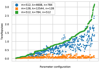
Figure 1: The performance of all different kernel configurations for three sets of input sizes on the AMD R9 Nano GPU, with varying matrix sizes from square to rectangular. Multiplying small reasonably square matrices performs best overall and favors large tile sizes, while tall skinny matrices perform poorly in all configurations.

As an example of this, on the R9 Nano the best performing configuration (tiles (8, 4, 4), work-group (16, 16) for m=512, k=784, n=512, batch=16) achieves 3160 gigaflops per second, while the worst configuration (tiles (1, 8, 1), work-group (8, 8) for m=32, k=12321, n=27, batch=1) only achieves 13 Gflops/sec. The best configurations for the small cases are the ones that use the most threads and so achieve the highest utilisation of the GPU, while the best configurations for large problems are the ones that reuse the most data without spilling registers. As the numbers of threads and numbers of registers are device specific, these are the things that an automated kernel deployment system would have to implicitly learn from the dataset.

Figure 1 shows the performance for three different sets of input matrix sizes. The more square matrices (m=512, k=784, n=512) allowed the kernels to perform best, but it only achieved optimal performance in a very small number of kernel configurations. In this case, of the 640 possible configurations only 55 achieved over 2 teraflops/sec and only 7 of those achieved over 3 teraflops/sec. This highlights the importance of tuning the kernel parameters and ensuring that the best parameters are available in a library.

The second results in Figure 1 from a more rectangular set of input matrices (m=512, k=4608, n=784) have three kernel configurations that achieve over 2 teraflops/sec. All three of these kernel configurations achieve over 3 teraflops/sec with the square input sizes, but the best performing configuration for the square inputs achieves less than 1.4 teraflops/sec for the rectangular input sizes. The third set of results correspond to an input set with a very large number of elements to accumulate, and as discussed above the kernel used is not optimized for these cases and so performs poorly overall.

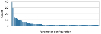
(a) AMD R9 Nano

(b) Intel i7-6700K CPU

Figure 2: The number of times a configuration of kernel parameters achieves optimal performance in the dataset. For the AMD GPU, one configuration is best in 39 cases, but 80 distinct configurations are best in at least one case. For the Intel CPU the top three configurations are best in 35, 28 and 25 cases respectively and 68 are best in at least one case.

The challenge faced by an automated kernel selection program is that many different configurations obtain the best performance for different matrix sizes. Figure 2 shows that while there are a small number of configurations that perform best in a large number of cases, there is a long tail where many other configurations also perform best in at least one of the benchmarks. This long tail illustrates the problem with pruning the number of configurations required to deploy within a library, and suggests that any such pruning will result in some loss of performance. The goal of this paper is to determine whether an automated solution can minimize this loss in performance.

The dataset and the corresponding code is available online [27]. The machine learning routines were provided by scikit-learn [28].

3.3 Determining the target number of configurations

As discussed in Section 2.1 a SYCL library cannot deploy an unlimited number of kernels, as they are embedded within the library as binary blobs. As such the kernels that should be deployed must be carefully selected to provide as much performance as possible. The number of kernels to deploy could be determined through trial and error by investigating the achievable performance of different numbers of kernels. A more tractable approach would be to explore the variance within the dataset and use that to estimate how many kernels may encapsulate that variance.

Principal component analysis (PCA) [29, 30] finds a new coordinate system for the dataset that concentrates the variance into as few dimensions as possible. In this way these principal dimensions contain the most distinguishing information about the dataset. Figure 3 shows the amount of total variance in the dataset that is accounted for by each of the components identified by PCA. This highlights that the data is fairly structured and that the majority of the variance is encapsulated within a small number of components.

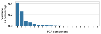
(a) AMD R9 Nano

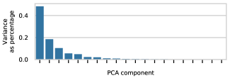
(b) Intel i7-6700K CPU

Figure 3: The percentage of the variance of the dataset accounted for by each PCA component. For the AMD GPU over 80% of the variance is accounted for in the 4 main components, 90% is accounted for in 7 components, and 95% in 14. For the Intel CPU 4 components account for 80% of the variance, 6 components for 90% and 11 components for 95%.

As PCA shows that most of the dataset’s variance can be encapsulated in less than 15 components we study how much performance can be encapsulated when providing at most 15 kernels. We compare the performance that is achievable when the number of kernels that would be deployed in a library varies between 4 and 15.

3.4 Normalization method

For each set of matrix sizes, the benchmarks measured the performance as gigaflops per second for each kernel. This gives 640 floating point values describing the performance, ranging from 0 to the maximum Gflops/sec of the device.

When comparing the performance of kernels for fixed matrix sizes, it is helpful to consider the comparative performance of the kernels instead of the raw flops/s achieved. By normalizing the data to only show the comparative performance, the data is easier for an automated system to understand. Such a normalization technique should map the performance to a value between 0 and 1, with the best performing kernels valued at or close to 1, while poor performing kernels have a value closer to 0.

In the original work, the only normalization technique considered was to scale the performance results relative to the performance of the kernel that performed best. The normalized value is obtained by dividing the achieved performance by the maximal performance for a fixed input. This provides a uniform mapping that preserves the relative performance between all kernels.

As the kernel selection process should infer more from the better performing kernels than the worst performing kernels, and hopefully never tries to select kernels that give mediocre performance, we can normalize the data to only preserve the kernels that perform well. We study three different approaches of doing this.

The first approach is to use a raw cutoff point, so that all results under a certain threshold are clamped to 0. In the results below we consider a cutoff value at 90% of the peak performance, so all results that obtain less than 90% of the optimal performance for each set of inputs is set to 0. This introduces sparsity in the data but does not change any non-zero values, so they range between 0.9 and 1.

An extension of this is to rescale the normalized data after clamping the poorly performing kernels. This ensures that the values make full use of the 0 to 1 range but may encourage the models to discard good performing kernels that it thinks actually perform poorly. In the discussion below we refer to this as the standard cutoff normalization technique (as opposed to the raw cutoff).

A final approach studied is to use a modified sigmoid function to map the scaled values, with many of the less well performing kernels mapped to 0. The sigmoid function $f(x)=(1+\exp(50*(0.85-x)))^{-1}$ was constructed to map 85% performance to 0.5 with all values less than 80% mapped to less than 0.1.

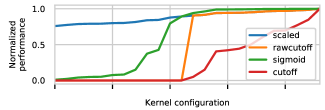
Figure 4: Comparison of different data normalization techniques for the best performing set of input sizes for the AMD GPU.

Figure 4 shows the effects these normalization techniques have on the best performing set of inputs for the AMD GPU, with the raw performance shown in Figure 1. As the normalization techniques all clamp low performing kernel configurations to zero, only the configurations achieving over 75% of the performance of the best configuration are shown.

4 Kernel selection

The techniques in this paper to deploy kernels in SYCL libraries is made up of two steps. First the kernel configurations should be selected, and then a simple model is constructed to choose which of these configurations to use at runtime for a given problem. As SYCL kernels are embedded into the library as binaries it is impractical to include a large number of kernels. In order to balance performance and binary size the number of kernels must be pruned to those that give the best performance on a range of different problems.

The initial selection of kernels is done using unsupervised clustering of the dataset. For a given set of matrix sizes the dataset provides performance information for each of the 640 kernel configurations. This performance information can be represented as a point in 640-dimensional space, though as the raw times vary between matrix sizes it is useful to normalize these coordinates.

Matrix sizes that have similar performance characteristics will naturally end up with similar coordinates, and so clustering techniques can be used to group these together. By considering these clusters of similarly performing matrix sizes we can extract which kernels give the best performance.

4.1 Clustering techniques

There are many unsupervised machine learning clustering techniques available which try to extract meaning directly from the data. These each have different behaviors and consider different aspects of the data, so may extract widely varying sets of kernels.

4.1.1 $K$-means clustering

A relatively simple clustering method is $k$-means clustering, which is an iterative method to find $k$ centroids that minimize the distance from each points in the dataset to their closest centroid. This method is effective when the clusters have shapes that are close to the unit ball in the coordinate space, however if the cluster shapes are less regular or intertwined the method will struggle to separate the clusters.

4.1.2 PCA and $k$-means clustering

To help get around this, the coordinate space of the dataset can be transformed to help separate the clusters. One approach to do this is using Principal Component Analysis to reduce the dimensionality of the dataset and concentrate the variance of the dataset by making use of the full range of values in each of the new dimensions, then using $k$-means clustering on this transformed data.

4.1.3 Spectral clustering

Another similar approach is to use a spectral transformation before using $k$-means clustering. A similarity graph of the coordinates in the dataset can be represented as an adjacency matrix. The eigenvectors of the Laplacian of this matrix provide new coordinates that can be clustered using $k$-means.

4.1.4 HDBScan

Density based methods can also be used to cluster data, which use the density of the data to establish the boundaries between clusters. HDBScan [31, 32] is an example of such a clustering method that uses a hierachical tree structure to construct the clusters and provide better estimates of outlying data.

Unlike the other clustering methods, HDBScan does not provide a parameter for the number of target clusters, rather providing however many clusters it finds based on its other hyperparameters. In order to limit the numbers of clusters we compute the numbers of clusters for a sweep of the hyperparameters and in the following use whichever values gave the correct number of clusters.

4.1.5 Decision tree

While not a clustering method, decision trees can be used to choose a subset of a dataset by artificially limiting the number of leaf nodes in the tree. A decision tree can be trained as a regression solver that maps the input matrix sizes to the vector of performance data. Unlike the clustering methods, this takes into account the matrix sizes rather than just the performance data. Each leaf node then ends up being a performance vector which is an approximate representative of the performance vector for all input sizes that end up at that node in the tree.

4.2 Selecting the kernels to deploy

To compare the effectiveness of clustering methods for selecting kernel configurations to deploy in a library we explored their outcomes given the benchmark dataset. We used a selection method of choosing the kernels that gave best performance by count. This Top-N method is a formulation of the methods used when previously selecting the kernels manually, and serves as a useful baseline to see how differently more advanced methods perform.

The clustering methods provide either representatives of the clusters, such as the centroids of the $k$-means clusters, or just the cluster labels for each of the data entries. When there are representatives of the clusters, these can be used to select an optimal kernel by looking at which kernel configuration performs best for the representative. When the full cluster is provided the optimal kernel is computed by taking the geometric mean of all elements in the cluster and choosing the best performing configuration of this mean set of values.

4.3 The results

The dataset was split into training and test subsets, allowing a comparison of how well the techniques generalize to previously unseen matrix sizes. Each proposed technique used the training dataset to select a fixed number of kernel configurations and the test dataset was used to evaluate what percentage of the optimal performance could be achieved by only considering those selected kernels.

The optimal performance of the test data is given by the benchmark data and normalized to between 0 and 1. A geometric mean of each value for the best performing kernel out of the selection was computed with all entries of the test dataset to give this final performance figure.

Figure 5: The performance of each pruning technique in Section 4 as a percentage of the optimal obtainable performance for the AMD R9 Nano GPU, comparing the normalization techniques discussed in Section 3.4.

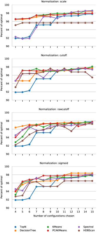
Figure 6: The performance of each pruning technique in Section 4 as a percentage of the optimal obtainable performance for the Intel i7-6700K CPU, comparing the normalization techniques discussed in Section 3.4.

Figure 5 shows the percentage of the optimal performance obtained by the different clustering techniques on the AMD GPU for the four different normalization techniques discussed in Section 3.4. The machine learning methods all perform better than the Top-N method of selecting the kernels based on those that perform best by count, except when the number of kernels selected gets very large. Some of the selection methods perform almost as well when selecting as few as 6 kernels, and don’t improve much as the number of kernels increases. This suggests that there are a small number of kernels that perform well for a wide range of input sizes, but that are not the ones that actually perform best for a large number of inputs.

For example when the number of kernels is limited to 4, the 4 top kernels by count are:

• Tiles (4, 8, 4), work-group (16, 16)

• Tiles (4, 8, 4), work-group (8, 16)

• Tiles (4, 8, 4), work-group (8, 32)

• Tiles (8, 4, 4), work-group (8, 32)

The tile sizes are all similar, with slightly different work-group sizes. These configurations perform similarly, and must perform well for some of the most common input sizes. However they do not perform well on the large number of less optimal input sizes, and so overall this selection gives poor performance. In comparison the decision tree selection is:

• Tile (2, 8, 1), work-group (8, 32)

• Tile (2, 8, 4), work-group (16, 16)

• Tile (4, 4, 4), work-group (8, 32)

• Tile (4, 8, 4), work-group (8, 32)

It includes only one of the top performing configurations, but this allows the overall kernel selection to be better suited to the different corner cases. These much more varied configurations therefore give better performance across a wider range of the input sizes.

All clustering methods performed well for the standard scaled normalization, though the Spectral clustering method performed worst after TopN. For the more sparse normalization techniques the performance of the clustering methods start to become more varied. Both the decision tree and k-means methods appear to perform well across the different normalization techniques, while the performance of HDBScan can vary.

This is promising for extending this data to the much more sparse data that would be generated by other auto-tuning techniques that run benchmarks of many fewer configurations. In these cases the data will naturally be much more sparse than the brute force dataset, and these normalization techniques mimic the data that might be obtained from these approaches.

The clustering methods most affected by normalization method are HDBScan and spectral clustering. When the data becomes more sparse these methods appear to select less optimal kernels and therefore gain worse performance overall. In addition HDBScan was the hardest to train, as the numbers of clusters cannot be specified as a parameter, so a parameter search is required to select the best options to limit the numbers of kernels.

Figure 6 shows the same data but for the Intel i7-6700K CPU. In the benchmarks this device was more consistent in the performance that it achieved for different input sizes. As such all kernel selection techniques performed significantly better than for the AMD GPU, where there was much more variation in the obtained performance.

In these benchmarks, the HDBScan density based clustering technique performed surprisingly poorly and the results varied significantly depending on the number of kernels. For the standard normalization technique all tested parameters gave only 4 or 5 kernels.

The decision tree clustering method performed well for the AMD data, often achieving among the best performance, however for the CPU this is not the case. It seemed to lose the least performance on the raw cutoff normalization scheme, but for all other normalization schemes the decision tree tends to be outperformed by the other clustering methods.

4.4 Clustering conclusions

The baseline option of choosing the kernels by which appear to be best most often is a weak approach. The more intelligent clustering methods outperformed this in the majority of cases, as they consider the distribution of the data more generally and use that to select the kernels that provide better performance across a wide range of inputs.

The aim for the kernel clustering is to automatically prune the number of kernels to provide in a library. As such the chosen solution should provide good performance regardless of the device or normalization scheme. The decision tree, spectral clustering and HDBScan clustering give varied performance across the devices and types of normalization, whereas the K-means and PCA+$K$-means clustering methods provide stable and good results. There are definitely cases where these relatively simplistic clustering techniques do not perform as well as some others, but the difference is rarely large.

5 Deploying the kernels

Selecting which kernels to deploy in a library is only half the story as our goal is to be able to support any inputs required by our users. This requires a method to map the user’s inputs to the best kernel configuration provided by the library. Such a process must be carried out before launching each kernel to ensure that the optimal choice is made at each point. This means that the selection process must be both effective and inexpensive to compute; there is little point gaining a small performance boost in the kernel if it is outweighed by time spent in a large classification system.

5.1 Classifiers

The previous sections investigated how to limit the number of kernel configurations that should be provided in a library. Selecting which of these kernels to run is a classification problem that maps the input matrix sizes to the optimal kernel configuration. For each entry in our dataset we can see which of the chosen kernels provides the best performance, and train a classifier to do this selection using standard supervised learning techniques.

There are many different techniques for classification using machine learning. The classifier will have to be run each time a new matrix multiplication is launched by the library and so the main challenge is to balance the effectiveness of the classifier with the time taken to make a classification. More complicated state of the art classifiers like neural networks may be very effective, but they are also computationally expensive and so would be a poor choice to integrate in this way. Decision trees on the other hand are easy to implement in a performant way and easy to integrate in a library, as they can be implemented as a series of nested if statements within the kernel launcher. If a decision tree can effectively infer the best kernel to use for unseen matrix sizes then this would be an ideal solution to use.

To establish whether this is the case, we compare the effectiveness of three decision trees to other classification techniques. The decision trees have increasing limits on the depth and numbers of samples allowed for leaf nodes. Varying these parameters helps establish how much the decision tree might be overfitting. Deeper trees can fit better to the training data, but will potentially overfit to suit the training data and perform poorly on previously unseen inputs.

The three decision trees are signified A, B and C. Decision tree A has no limit on the maximum depth and allows splitting down to single sample leaf nodes if required. Decision tree B has a maximum depth of 6 and requires leaf nodes to have at least 3 samples, while decision tree C has a maximum depth of 3 and requires at least 4 samples at the leaves. There are many other possible combinations of parameters, however additional tuning of these risk overfitting to the testing data set.

Table 1: The performance results for the classifiers as a percentage of the absolute optimal performance, for the kernel configurations selected by PCA+$K$-means for the AMD R9 Nano. Note that the maximum achievable performance for the selection of configurations is limited to 91.19%, 94.62%, 94.94% and 96.89% for the 5, 6, 8 and 15 configurations respectively.

	Number of configurations
Classifier	5	6	8	15
DecisionTreeA	88.16	86.82	85.53	85.64
DecisionTreeB	86.10	90.62	83.21	83.01
DecisionTreeC	84.56	85.39	82.30	83.66
1NearestNeighbor	77.37	78.93	77.79	75.48
3NearestNeighbor	78.15	78.64	76.85	76.82
7NearestNeighbor	75.38	74.85	75.08	77.39
LinearSVM	68.68	74.46	67.31	77.62
RadialSVM	70.93	70.93	70.93	70.93
RandomForest	86.91	89.31	87.60	83.96
MLP	63.61	56.35	64.39	62.99

Table 2: The performance results for the classifiers as a percentage of the absolute optimal performance, for the kernel configurations selected by PCA+$K$-means for the Intel i7-6700K CPU. Note that the maximum achievable performance for the selection of configurations is limited to 96.55%, 96.65%, 97.34% and 97.95% for the 5, 6, 8 and 15 configurations respectively.

	Number of configurations
Classifier	5	6	8	15
DecisionTreeA	91.65	92.59	93.50	92.29
DecisionTreeB	93.14	91.86	93.87	90.15
DecisionTreeC	92.26	91.11	91.51	91.28
1NearestNeighbor	91.36	91.36	91.40	89.73
3NearestNeighbor	91.18	90.26	91.61	86.42
7NearestNeighbor	88.00	90.15	89.22	87.96
LinearSVM	84.18	76.20	88.32	85.64
RadialSVM	80.49	83.80	78.55	83.80
RandomForest	93.65	93.90	93.26	93.85
MLP	74.30	79.23	79.23	76.88

Nearest neighbor is another relatively simple classification technique that classifies an input based on which of the training inputs are closest to it. As such it requires that the training dataset be stored alongside the classifier to compute which data points are the input’s neighbors. As such it would be infeasible to deploy within the library but provides a useful comparison for what similar classifiers can achieve.

Other classifiers are more complex and require significantly more computation to infer a class from an input. Classifiers like SVM, which computes the vectors that separate the classes, and random forest ensembles, made up of multiple decision trees that are combined together, can potentially provide better performance but would require more work on the host when choosing the kernel to launch.

The comparisons made between these classifiers considered how well they could infer the optimal kernel given the subset of kernels provided by the pruning techniques discussed in Section 4. As the choice of kernels is limited to this subset the maximum achievable performance is not 100%.

Tables 1 and 2 show the relative performance of the different classification methods for a range of possible kernel configurations. Overall the decision tree classification methods perform well, in many cases significantly better than the more computationally expensive methods.

One of the more surprising observations here is that the performance does not improve as the number of classes does, despite the theoretical maximum achievable performance increasing. The absolute best performance for both devices was obtained with just 6 kernel configurations, and the decision tree obtaining best performance for either 6 or 8 kernel configurations. While the additional kernel choices may allow higher theoretical performance, the models seem to struggle to differentiate between similar inputs that would require different kernels. As such having the extra choice actually hinders the model’s performance rather than allowing it to achieve better performance.

When comparing the three different decision tree configurations, the performance data does not support the theory that the tree may overfit to the training data. The more limited trees (B and C) tend to perform worse than the unlimited decision tree (A), though the numbers are not clear. When integrating the decision tree into the SYCL library it is helpful to provide some limits, so as to avoid heavily nested if statements and branching code.

6 Testing a full ML model

This work was carried out to help provide general purpose compute libraries to accelerate machine learning applications. Comparing the inference time of a machine learning model using these techniques to similar libraries that use ore manual tuning techniques can show the efficacy of this work.

One of the popular image classification models a few years ago was VGG16 [24], developed at the Oxford Visual Geometry Group in 2015. By modern standards it is a simple neural network made up of 16 convolutional and pooling layers. Despite the small number of layers it has more parameters than most modern networks with 138 million, as the convolutional layers have many features.

While no longer state of the art, this model is still regularly used by machine learning practitioners and much simpler than more recent image classification networks, making it a good candidate to use to evaluate the performance of the kernel selection process. Comparing the performance of individual kernels provides a good proxy to determine how well a system will perform, but an evaluation on the full system will help uncover any assumptions and shortcomings that would not be visible at the micro-benchmark scale.

A SYCL-DNN sample implements the VGG16 network in SYCL using the pretrained weights provided by the Keras Applications [33] Python module. It can perform image classification based on the ImageNet dataset, providing the class of an input image from the 1000 different ImageNet classes. This pretrained network achieves 71.3% performance classifying the top class of an image in the ImageNet dataset. It is not the best performing model available through Keras but is one of the simplest to implement.

In addition to testing the performance of this network on the devices discussed earlier in this paper, we also tested two additional OpenCL devices. The kernels used were tuned for each device using the methods discussed above and the resulting deployment and selection algorithms were integrated into SYCL-DNN.

The devices used to test these techniques were:

• AMD R9 Nano GPU

• Intel i7-6700K CPU

• Intel HD 530 Gen9 GPU

• ARM Mali G71 GPU

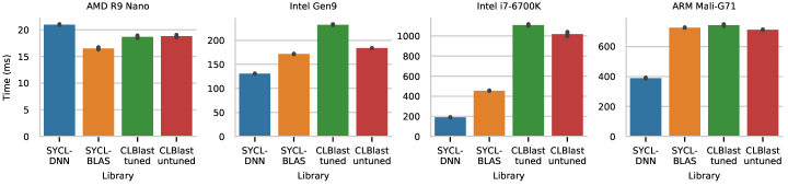
Figure 7: The inference time in miliseconds of a single image using the VGG16 model implemented using SYCL-DNN and different matrix backends when run on different devices.

6.1 Library comparisons

SYCL-DNN allows users to specify different backends that provide the matrix multiplication routines used in neural networks. The library provides its own matrix multiplication, but if a platform has access to a BLAS or other matrix library then it can be easily integrated to make use of these optimized routines. This functionality was used to provide comparisons to the tuned SYCL-DNN matrix multiplication kernels, using both a SYCL-BLAS [5] backend and a CLBlast [4] backend.

SYCL-BLAS is another library developed by Codeplay to provide basic linear algebra kernels. Designed with expression trees and templated kernels it allows users to easily fuse kernels together at compile time, reducing the need to load and store data between kernel launches, and is optimized for a range of devices. SYCL-BLAS provides a number of different matrix multiplication routines, including ones utilizing local (or shared) memory and ones designed for tall skinny matrices that compute partial results which are combined in a final reduction. These kernels are significantly more sophisticated than the simple kernel studied in this paper, however the parameters are all tuned by hand requiring significant developer effort and time.

CLBlast is an OpenCL based BLAS library designed to be performant on a wide range of OpenCL devices. It includes an automated tuning system to select the optimal kernels for different devices, though this system is limited to selecting the single best kernel for each device. Before running this benchmark, the CLBlast library was tuned for each of the benchmark devices used. Similarly to SYCL-BLAS, the CLBlast library contains multiple implementations of matrix multiplication kernels to help achieve performance for different matrix shapes.

6.2 Results

The model was executed a number of times to accurately measure the time of completion. A single image was used as an input, and the model classifies the contents of that image. The weights and initial image are all transferred to the compute device before starting timing, so the benchmark time only includes the computation and not data transfer. The SYCL-DNN matrix multiplication routine was tuned to use 8 kernel configurations per device selected using PCA+$K$-means and a decision tree based runtime selection process. As discussed in Sections 4 and 5 these approaches give good performance for different matrix sizes and devices.

Figure 7 shows the execution time to compute one inference using the VGG16 model. The different devices perform significantly differently as would be expected as they have vastly different compute resources available.

The AMD R9 Nano performed an inference in less than 20ms using the optimized and tuned matrix multiplication kernels from SYCL-BLAS and CLBlast. This GPU along with this particular machine learning model was one of the main targets of optimization during the development of SYCL-BLAS so it is expected that it performs well, outperforming both the kernel studied in this paper and CLBlast. The SYCL-DNN kernel achieved times that were not far off the others, despite the kernel being much simpler than those in the heavily optimized libraries and not making use of the GPU’s fast local memory.

By default CLBlast will use generic tuning parameters based on similar devices, so for the R9 Nano the parameters are based on similar AMD cards. Tuning CLBlast for this specific GPU using the provided tuning tools didn’t provide any benefit, though the actual kernels used did change. For the other devices the tuning often had a negative impact on the performance of CLBlast. This is likely to be a result of the limited way that the tuning works causing it to optimize for best results on matrix sizes that differ from those used in the VGG16 model. The GEMM routine in particular is tuned for single matrices of size 1024x1042 and 256x256, whereas the inputs to GEMM used in the model have a batch size of 16 and vary from 12544x64 to 512x512.

For the Intel CPU and integrated GPU the SYCL-DNN kernel actually performed better than the optimized libraries. The CPU has very different performance characteristics and compute resources to any of the GPUs, and CLBlast particularly struggles to adapt to this.

Both SYCL-BLAS and CLBlast achieve similar performance on the ARM Mali GPU, taking over 700ms per inference. SYCL-DNN on the other hand achieves under 400ms per inference, as it makes use of 4 different configurations out of the chosen 8. This variety of possible kernel configurations allows the library to hand the different matrix sizes where the other libraries only use a single kernel configuration.

One of the areas where the SYCL-DNN kernels are at a disadvantage to the other libraries is in the final fully connected layers in the model. These fully connected layers are implemented as a matrix multiplication, but when using a single image the activation tensor is actually a one dimensional vector rather than a matrix. As such it is much more efficient to use a dedicated matrix-vector multiplication routine common in BLAS libraries. The SYCL-DNN kernel is comparatively inefficient in this case, as it is designed to compute 2D tiles of the output, which would only be one-dimensional. Despite this, the library manages to provide sufficient performance on these operations that the automatically tuned SYCL-DNN kernels outperform the other libraries overall.

7 Conclusions

Auto-tuning allows libraries to achieve performance on a wide range of devices without requiring vast amounts of developer effort to adapt kernels and routines to new hardware. In this paper we used a matrix multiplication case study to evaluate some methods to allow auto-tuning to be deployed in compiled SYCL libraries, balancing binary size, performance and adaptability to unseen inputs.

Unsupervised machine learning techniques like clustering provide effective methods to reduce the large kernel parameter space for a wide range of different input sizes without sacrificing much performance. Some of these methods proved more reliable and resilient than others, with some of the more advanced methods like density based clustering methods struggling to provide performant kernels in some cases.

One of the concerns raised in the original paper [22] introducing these ideas was that the techniques may rely too heavily on the dense benchmark timing information. Intelligent auto-tuning techniques only sample from the very large kernel parameter space, while the data collected for this study used a comparatively small parameter space and so used a brute-force benchmarking technique. The normalization techniques discussed in Section 3.4 introduce sparsity into the data and Section 4 shows that while this does have an impact on the performance of the kernel selection routines, this difference is minimal. This is promising for extending these results to more complicated kernels that use more parameters that can take a larger range of values.

After selecting the kernels to deploy in the SYCL library, there needs to be a runtime routine to choose which of these kernels to execute for any given input. The techniques discussed in Section 5 show that decision trees can provide good performance, as well as being easy to implement and integrate into a library.

When integrated into SYCL-DNN, these techniques met or vastly exceeded other optimized BLAS libraries for a representative machine learning model. The performance was competitive on a range of devices, from powerful desktop GPUs through to embedded mobile GPUs, even though the kernels themselves are relatively simple and don’t use as many hardware features as those in the other libraries.

Overall these tuning and deployment techniques provide an efficient subset of all possible kernels where the kernels have to be provided in binary format as with SYCL. These completely automated approaches allow new devices to be supported with very little developer effort and relatively small code changes.

References

References

- [1] J. E. Stone, D. Gohara, G. Shi, OpenCL: A parallel programming standard for heterogeneous computing systems, Computing in Science Engineering 12 (3) (2010) 66–73. doi:10.1109/MCSE.2010.69.
- [2] SYCL: C++ single-source heterogeneous programming for OpenCL, https://www.khronos.org/sycl/, accessed: 2019-03-11.
- [3] clBLAS: A software library containing BLAS functions written in opencl, https://github.com/clMathLibraries/clBLAS, accessed: 2020-08-26.
-
[4]
C. Nugteren, CLBlast: A tuned
OpenCL BLAS library, in: Proceedings of the International Workshop on
OpenCL, IWOCL ’18, ACM, New York, NY, USA, 2018, pp. 5:1–5:10.
doi:10.1145/3204919.3204924.
URL http://doi.org/10.1145/3204919.3204924 - [5] SYCL-BLAS: An implementation of BLAS using the SYCL open standard, https://github.com/CodeplaySoftware/SYCL-BLAS, accessed: 2019-04-09.
-
[6]
J. I. Aliaga, R. Reyes, M. Goli,
SYCL-BLAS: Leveraging
expression trees for linear algebra, in: Proceedings of the 5th
International Workshop on OpenCL, IWOCL 2017, ACM, New York, NY, USA, 2017,
pp. 32:1–32:5.
doi:10.1145/3078155.3078189.
URL http://doi.org/10.1145/3078155.3078189 - [7] C. Nugteren, V. Codreanu, Cltune: A generic auto-tuner for OpenCL kernels, in: 2015 IEEE 9th International Symposium on Embedded Multicore/Many-core Systems-on-Chip, 2015, pp. 195–202. doi:10.1109/MCSoC.2015.10.
-
[8]
B. van Werkhoven, Kernel
tuner: A search-optimizing GPU code auto-tuner, Future Generation Computer
Systems 90 (2019) 347 – 358.
doi:10.1016/j.future.2018.08.004.
URL https://doi.org/10.1016/j.future.2018.08.004 - [9] T. L. Falch, A. C. Elster, Machine learning based auto-tuning for enhanced OpenCL performance portability, in: 2015 IEEE International Parallel and Distributed Processing Symposium Workshop, 2015, pp. 1231–1240. doi:10.1109/IPDPSW.2015.85.
- [10] J. Bergstra, N. Pinto, D. Cox, Machine learning for predictive auto-tuning with boosted regression trees, in: 2012 Innovative Parallel Computing (InPar), 2012, pp. 1–9. doi:10.1109/InPar.2012.6339587.
-
[11]
D. Grewe, Z. Wang, M. P. O’Boyle,
Portable mapping of data
parallel programs to opencl for heterogeneous systems, in: 2013 IEEE/ACM
International Symposium on Code Generation and Optimization (CGO), IEEE
Computer Society, Los Alamitos, CA, USA, 2013, pp. 1–10.
doi:10.1109/CGO.2013.6494993.
URL https://doi.org/10.1109/CGO.2013.6494993 - [12] W. F. Ogilvie, P. Petoumenos, Z. Wang, H. Leather, Active learning accelerated automatic heuristic construction for parallel program mapping, in: 2014 23rd International Conference on Parallel Architecture and Compilation Techniques (PACT), 2014, pp. 481–482. doi:10.1145/2628071.2628128.
- [13] T. D. Han, T. S. Abdelrahman, Automatic tuning of local memory use on gpgpus, in: ADAPT Workshop proceedings, 2015, Vol. 1410.0759, 2014. arXiv:1410.0759.
-
[14]
B. van Werkhoven, J. Maassen, H. E. Bal, F. J. Seinstra,
Optimizing convolution
operations on GPUs using adaptive tiling, Future Generation Computer
Systems 30 (2014) 14 – 26, special Issue on Extreme Scale Parallel
Architectures and Systems, Cryptography in Cloud Computing and Recent
Advances in Parallel and Distributed Systems, ICPADS 2012 Selected Papers.
doi:10.1016/j.future.2013.09.003.
URL https://doi.org/10.1016/j.future.2013.09.003 - [15] Y. Li, J. Dongarra, S. Tomov, A note on auto-tuning GEMM for GPUs, in: G. Allen, J. Nabrzyski, E. Seidel, G. D. van Albada, J. Dongarra, P. M. A. Sloot (Eds.), Computational Science – ICCS 2009, Springer Berlin Heidelberg, Berlin, Heidelberg, 2009, pp. 884–892.
-
[16]
A. Nukada, S. Matsuoka,
Auto-tuning 3-D FFT library
for CUDA GPUs, in: Proceedings of the Conference on High Performance
Computing Networking, Storage and Analysis, SC ’09, ACM, New York, NY, USA,
2009, pp. 30:1–30:10.
doi:10.1145/1654059.1654090.
URL http://doi.org/10.1145/1654059.1654090 - [17] A. Mametjanov, D. Lowell, C. Ma, B. Norris, Autotuning stencil-based computations on GPUs, in: 2012 IEEE International Conference on Cluster Computing, 2012, pp. 266–274. doi:10.1109/CLUSTER.2012.46.
-
[18]
Y. Zhang, F. Mueller,
Auto-generation and auto-tuning
of 3D stencil codes on GPU clusters, in: Proceedings of the Tenth
International Symposium on Code Generation and Optimization, CGO ’12, ACM,
New York, NY, USA, 2012, pp. 155–164.
doi:10.1145/2259016.2259037.
URL http://doi.org/10.1145/2259016.2259037 -
[19]
M. Abadi, A. Agarwal, P. Barham, E. Brevdo, Z. Chen, C. Citro, G. S. Corrado,
A. Davis, J. Dean, M. Devin, S. Ghemawat, I. Goodfellow, A. Harp, G. Irving,
M. Isard, Y. Jia, R. Jozefowicz, L. Kaiser, M. Kudlur, J. Levenberg,
D. Mané, R. Monga, S. Moore, D. Murray, C. Olah, M. Schuster, J. Shlens,
B. Steiner, I. Sutskever, K. Talwar, P. Tucker, V. Vanhoucke, V. Vasudevan,
F. Viégas, O. Vinyals, P. Warden, M. Wattenberg, M. Wicke, Y. Yu,
X. Zheng, TensorFlow: Large-scale
machine learning on heterogeneous systems, software available from
tensorflow.org (2015).
URL https://www.tensorflow.org/ - [20] T. Chen, M. Li, Y. Li, M. Lin, N. Wang, M. Wang, T. Xiao, B. Xu, C. Zhang, Z. Zhang, Mxnet: A flexible and efficient machine learning library for heterogeneous distributed systems, ArXiv 1512.01274. arXiv:1512.01274.
- [21] S. Chetlur, C. Woolley, P. Vandermersch, J. Cohen, J. Tran, B. Catanzaro, E. Shelhamer, cudnn: Efficient primitives for deep learning, CoRR abs/1410.0759. arXiv:1410.0759.
- [22] J. Lawson, Towards automated kernel selection in machine learning systems: A SYCL case study, in: 2020 IEEE International Parallel and Distributed Processing Symposium Workshops (IPDPSW), 2020, pp. 475–478. doi:10.1109/IPDPSW50202.2020.00086.
-
[23]
R. Burns, J. Lawson, D. McBain, D. Soutar,
Accelerated neural networks on
OpenCL devices using SYCL-DNN, in: Proceedings of the International
Workshop on OpenCL, IWOCL’19, ACM, New York, NY, USA, 2019, pp. 10:1–10:4.
doi:10.1145/3318170.3318183.
URL http://doi.org/10.1145/3318170.3318183 - [24] K. Simonyan, A. Zisserman, Very deep convolutional networks for large-scale image recognition, CoRR abs/1409.1556. arXiv:1409.1556.
- [25] K. He, X. Zhang, S. Ren, J. Sun, Deep residual learning for image recognition, in: 2016 IEEE Conference on Computer Vision and Pattern Recognition (CVPR), 2016, pp. 770–778. doi:10.1109/CVPR.2016.90.
- [26] M. Sandler, A. Howard, M. Zhu, A. Zhmoginov, L. Chen, MobileNetV2: Inverted residuals and linear bottlenecks, in: 2018 IEEE/CVF Conference on Computer Vision and Pattern Recognition, 2018, pp. 4510–4520. doi:10.1109/CVPR.2018.00474.
- [27] Towards automated kernel selection in macine learning systems: Supplementary code and dataset, https://github.com/jwlawson/tuning_kernels, accessed: 2020-02-07.
- [28] F. Pedregosa, G. Varoquaux, A. Gramfort, V. Michel, B. Thirion, O. Grisel, M. Blondel, P. Prettenhofer, R. Weiss, V. Dubourg, J. Vanderplas, A. Passos, D. Cournapeau, M. Brucher, M. Perrot, E. Duchesnay, Scikit-learn: Machine learning in Python, Journal of Machine Learning Research 12 (2011) 2825–2830.
-
[29]
K. Pearson, LIII. On lines
and planes of closest fit to systems of points in space, The London,
Edinburgh, and Dublin Philosophical Magazine and Journal of Science 2 (11)
(1901) 559–572.
doi:10.1080/14786440109462720.
URL https://doi.org/10.1080/14786440109462720 -
[30]
M. E. Tipping, C. M. Bishop,
Probabilistic principal component
analysis, Journal of the Royal Statistical Society. Series B (Statistical
Methodology) 61 (3) (1999) 611–622.
URL http://www.jstor.org/stable/2680726 - [31] R. J. G. B. Campello, D. Moulavi, J. Sander, Density-based clustering based on hierarchical density estimates, in: J. Pei, V. S. Tseng, L. Cao, H. Motoda, G. Xu (Eds.), Advances in Knowledge Discovery and Data Mining, Springer Berlin Heidelberg, Berlin, Heidelberg, 2013, pp. 160–172.
- [32] L. McInnes, J. Healy, Accelerated hierarchical density based clustering, in: 2017 IEEE International Conference on Data Mining Workshops (ICDMW), 2017, pp. 33–42. doi:10.1109/ICDMW.2017.12.
- [33] Keras applications: Reference implementations of popular deep learning models., https://github.com/keras-team/keras-applications, accessed: 2020-08-27.