Formation of dust filaments in the diffuse envelopes of molecular clouds

Abstract

The path to understanding star formation processes begins with the study of the formation of molecular clouds. The outskirts of these clouds are characterized by low column densities that allow the penetration of ultraviolet radiation, resulting in a non-negligible ionization fraction and the charging of the small dust grains that are mixed with the gas; this diffuse phase is then coupled to the ambient magnetic field.
Despite the general assumption that dust and gas are tightly correlated, several observational and theoretical studies have reported variations in the dust-to-gas ratio toward diffuse and cold clouds.
In this work, we present the implementation of a new charged particles module for analyzing the dust dynamics in molecular cloud envelopes. We study the evolution of a single population of small charged grains (0.05 $\mu$m) in the turbulent, magnetized molecular cloud envelope using this module. We show that variations in the dust-to-gas ratio arise due to the coupling of the grains with the magnetic field, forming elongated dust structures decoupled from the gas. This emphasizes the importance of considering the dynamics of charged dust when simulating the different phases of the interstellar medium, especially for star formation studies.

1 Introduction

Molecular clouds (MCs) are the galactic reservoirs of molecular material where star formation takes place. It is therefore necessary to understand their formation and evolution if one aspires to comprehend the physical processes involved in star formation.

It is known that MCs are formed from a more diffuse medium that becomes thermally unstable (see the recent reviews by e.g. Ballesteros-Paredes et al. 2020 and Chevance et al. 2020). Their turbulent nature (Elmegreen & Scalo, 2004) is inherited from the parental gas (Meidt et al., 2018; Kruijssen et al., 2019), and is mantained by several processes both at large and small scales, such as supernova explosions (Padoan et al., 2016; Bacchini et al., 2020) or stellar jets (Federrath, 2015; Offner & Liu, 2018). This turbulence, together with the pervasive galactic magnetic field, plays a fundamental role in the fragmentation of the cloud and the formation of dense gas filaments where stars are actually formed (Myers & Goodman, 1988; Fiege & Pudritz, 2000; Nakamura & Li, 2008; Inutsuka et al., 2015).

MCs are formed from the accretion of warm, diffuse gas from the warm neutral medium (WNM), characterized by its atomic composition (mainly HI), temperatures of approximately 6000K, densities ranging from 0.2 - 0.5 cm^-3 (Ferrière, 2001) and ionization fractions of $\chi\sim 0.1$ (Klessen & Glover, 2016); these conditions are sustained in time due to the constant bombardement of the interstellar radiation field over the molecular gas. Therefore, MC envelopes share properties with the WNM, and they constitute the transition layers between the hot ionized gas of the diffuse interstellar medium (ISM) and the interiors of the clouds. The net charge of the species in the outskirts of these clouds favours their coupling with the galactic magnetic field, which act as a carrier of hydromagnetic waves (Balsara, 1996); they may also facilitate the penetration of cosmic rays inside the cloud (Ivlev et al., 2018).

A key ingredient in the transition from atomic to molecular gas is interstellar dust, which distribution seems to be correlated with that of the gas (Bohlin et al., 1978; Boulanger et al., 1996; Roman-Duval et al., 2010; Lenz et al., 2017). Despite representing only 1% in mass of the ISM, interstellar dust grains play a fundamental role in several physical phenomena. They act as catalysts in chemical reactions (Hollenbach & Salpeter, 1971; Cazaux & Tielens, 2004; Shingledecker et al., 2020), shield the interior of the clouds from the high energy ultraviolet (UV) radiation, and contribute to the thermal regulation of the cloud (Bakes & Tielens, 1994; Wolfire et al., 1995; Weingartner & Draine, 2001; Hocuk & Spaans, 2010)
Due to their composition, dust grains acquire a net charge in the presence of a radiation field (Weingartner & Draine, 2001); even in the densest regions of MCs, grains may be charged due to the action of cosmic rays (Ivlev et al., 2015). In MC envelopes, dust grains contribute to the magnetic field coupling and affect the propagation of hydromagnetic waves (Pilipp et al., 1987; Cramer & Vladimirov, 1997) and, in last instance, star formation (Nakano, 1998). It is then crucial to consider interstellar dust grains when studying the formation and evolution of MCs.

Over the last decade, our knowledge of the cold ISM has grown exponentially thanks to the results of dedicated missions such as Herschel (see e.g. André et al. 2010; Arzoumanian et al. 2011; Palmeirim et al. 2013) and Planck (Planck Collaboration et al., 2018a, b). However, the characterization of the diffuse ISM is more challenging, since it requires tracers sensitive to low column densities, such as ¹²CO (Falgarone & Phillips, 1996; Falgarone et al., 2005) or very high-resolution HI maps (Clark et al., 2014; Martin et al., 2015). An alternative approach, which is very time-consuming but provides a higher resolution, is to perform a spectroscopic survey of the neutral and ionized components of the ISM at optical and UV wavelengths (Savage & Sembach, 1991; Lallement et al., 2003; Redfield et al., 2004; Welsh et al., 2010).

With these ingredients, it seems that a full characterization of MCs may be within reach. However, observations give at most a line-of-sight averaged view of the processes involved in MC evolution and thus, to understand the underlying physics, numerical simulations of these processes are required.

It has been predicted that negatively charged grains may affect the star formation efficiency due to gyroresonance effects with MHD waves propagating inside MCs (Pilipp et al., 1987; Nakano, 1998; Falceta-Gonçalves et al., 2003; Hopkins et al., 2020). For instance, Chapman & Wardle (2006) demonstrated that C-type MHD shocks profiles are deeply affected by the presence of a population of charged grains; Pandey & Vladimirov (2019) have recently shown that the Kevin-Helmholz instability in MCs depends on the dust charge density and size distribution; and Wardle (2007) and Pinto et al. (2008) derived the modified coefficients for non-ideal MHD effects (Ohmic resistivity, and ambipolar and Hall diffusion) in the presence of charged dust grains. However, none of the abovementioned studies followed the numerical evolution of a MC in the presence of a population of dust.

The main trend has been to consider the aerodynamic drag of dust in the framework of protoplanetary disks (Bai & Stone, 2010; Price et al., 2018; Mignone et al., 2019). Up to the knowledge of the authors, the only ones that have included the physics of charged grains in their MHD simulations are Lee et al. (2017); they have devoted a series of papers to the exhaustive study of resonant instabilities that arise between gas and charged dust over different phases of the ISM when dust motions are driven by an external force (Hopkins & Squire, 2018; Seligman et al., 2019; Hopkins et al., 2020).

In this article, we study the dynamics of both gas and charged dust under conditions typical of a molecular cloud envelope with a modified version of the MHD code Athena (Stone et al., 2008). In Section 2 we present our implementation of the dynamics of charged dust. In Section 3, we present the numerical 2D model for the MC envelope (3.1) and analyze the local variations of the dust-to-gas ratio (3.2) as well as the dust filamentary structure (3.3). In Section 4, a discussion of the results is provided and the main results are highlighted in Section 5.

2 Numerical modeling of charged dust

We worked with the latest stable version of Athena (v4.2). This C-version has already implemented an aerodynamic particles module (Bai & Stone 2010, hereafter BS2010). In this section, we detail how we have expanded this module by adding the necessary equations that take into account the dynamics of charged dust. We have also carried out different tests for checking this new implementation that are detailed in Appendix A.

Apart from the traditional drag term characterized by the stopping time $t_{s}$ (Weidenschilling, 1977), we added two terms to the equation of motion of a charged particle that account for the Coulomb drag from charged gas species, and the Lorentz force:

$$\frac{d{\bf v}}{dt}=-\frac{{\bf v}-{\bf u}}{t_{s}}-\nu_{C}({\bf v}-{\bf u})+\frac{Z_{d}e}{m_{d}c}({\bf v}-{\bf u})\times{\bf B}$$ (1)

In the above equation, v is the velocity of the dust grain, u is the gas velocity, $t_{s}$ is the aerodynamic stopping time, $Z_{d}$ is the grain charge, $m_{d}$ is the dust mass, $c$ is the speed of light and the term $\nu_{C}$ is an additional drag term that accounts for Coulomb interactions between charged grains and ions/electrons in the plasma:

$$\nu_{C}=\frac{4}{3}\frac{\sqrt{2\pi}Z_{d}^{2}e^{4}\ln\Lambda n_{d}}{(kT)^{3/2}}\bigg{(}\frac{\delta}{\sqrt{m_{ion}}}+\frac{(1-\delta)}{\sqrt{m_{e}}}\bigg{)}$$ (2)

In this equation, $\ln\Lambda=\ln[(3kT/2e^{3})(kTm_{e}/\rho_{e}\pi)^{1/2}]$ is the Coulomb logarithm, $n_{d}$ is the density of charged dust grains, and $\delta=1$ if $Z<0$, $\delta=0$ otherwise; this means that negatively (positively) charged dust grains interact with the ions (electrons) in the gas. We disregarded the effect of the electric field derived from the magnetic field in the Lorentz force because we are mainly interested in studying the effects of first order terms.

We coupled the integration of the Lorentz force and the Coulomb drag in the semi-implicit integrator of BS2010, which is very similar to the Boris integrator (Boris, 1970) implemented by Lehe et al. (2009). Following the notation by BS2010, the equations to solve for the particle dynamics are:

$$\frac{d{\bf x}}{dt}={\bf v},~{}~{}\frac{d{\bf v}}{dt}={\bf a}[{\bf v},{\bf x},{\bf u}^{n+1/2}({\bf x})]$$ (3)

where we have grouped all the acceleration terms in eq. (1) under the term ${\bf a}$. Then, the velocity update can be computed using the predicted particle position ${\bf x^{\prime}}$ as:

$${\bf v}^{(n+1)}={\bf v}^{(n)}+h\Lambda^{-1}{\bf a}({\bf v}^{(n)},{\bf x^{\prime}},{\bf u}({\bf x^{\prime}})),~{}\Lambda=1-\frac{h}{2}\frac{\partial{\bf a}}{\partial{\bf v}}$$ (4)

where the Jacobian matrix for eq. (1) is:

$$\frac{\partial{\bf a}}{\partial{\bf v}}=\pmatrix{-\frac{1}{t_{s}}-\nu_{C}&Q_{m}B_{z}&-Q_{m}B_{y}\cr-Q_{m}B_{z}&-\frac{1}{t_{s}}-\nu_{C}&Q_{m}B_{x}\cr Q_{m}B_{y}&-Q_{m}B_{x}&-\frac{1}{t_{s}}-\nu_{C}}$$ (5)

In the above matrix, we have renamed the term $Z_{d}e/m_{d}c$ as $Q_{m}$ for simplicity.

The last consideration for the implementation of charged particles is the numerical timestep. In order to integrate accurately the oscillation of a charged particle, the timestep has to be considerably smaller than the particle’s Larmor time. As a compromise between numerical accuracy and computational cost, we have chosen the same value as that by Lee et al. (2017):

$$\Delta t=\frac{\rm CFL}{10}\min\bigg{(}\frac{m_{d}c}{Z_{d}e|{\bf B}|},\Delta t_{\rm MHD}\bigg{)}$$ (6)

where CFL is the Courant-Friedrichs-Lewy number and $t_{\rm MHD}$ is the timestep computed without considering the dust particles.

3 Simulations of a Molecular Cloud envelope

3.1 Numerical model

We solve with Athena the equations for isothermal, ideal MHD in 2D together with Eq. 1 for the dust dynamics in a box of length $L$ with periodic boundary conditions.

As a first step in the study of the dynamics of charged dust in MCs, we developed a very simple model of a MC envelope that responds to the common physical parameters of the WNM. The ambient gas is composed by HI at $T=6000K$ with an ionization fraction $\chi=0.1$; the magnetic field strength is chosen to be $B=10^{-6}$ G, in concordance with the measured values in the ISM of a few $\mu$m (Ferrière, 2001). The gas density is $n=10$ cm^-3, a selection justified by observational evidence (Blitz et al., 2007; Fukui et al., 2009, 2017).

The dust population is represented by 80,000 test particles that share the same properties: a radius of $a_{d}=5\times 10^{-6}$cm and an internal density of $\rho^{int}_{d}=1$g cm^-3. They are randomly distributed over the whole domain with a velocity taken from a Gaussian distribution with deviation $v_{th}$, the isothermal sound speed. For these grains, we computed an average electric charge under the assumption of statistical equilibrium of $Z=-17$ following the procedure described in Weingartner & Draine (2001); the intensity of the interstellar radiation field (Mathis et al., 1983) is considered to be $G=1$.

Initially, the medium is uniform in density, with the magnetic field parallel to the x-axis. The box size is chosen to be $L=1$ pc, a value that allows to resolve the apparent characteristic molecular gas filament widths of 0.1 pc (Arzoumanian et al., 2011) and, of more relevance for the present study, the width of HI fibers observed in the diffuse ISM (sizes below 0.04 pc, Clark et al. 2014): at the chosen resolution ($1024\times 1024$, see below), one pixel size corresponds to $1/1024\sim 9.76\times 10^{-4}$ pc. We introduced a turbulent spectrum in velocity as the superposition of four waves with wavelengths $\lambda_{0}=L/24$, $\lambda_{1}=26L/72$, $\lambda_{2}=49L/72$, $\lambda_{3}=L$ and wave amplitude $u_{0}=v_{th}(k_{n}/k_{0})^{3/2}$:

$$u_{x}=u_{0}\sum_{n=0}^{3}\cos(k_{n}y)$$

$$u_{y}=u_{0}\sum_{n=0}^{3}\sin(k_{n}y)$$ (7)

$$u_{z}=0$$

The wave spectrum has been chosen such that the number of waves ($N_{waves}=4$) is large enough to produce a turbulent state in the gas, but small enough to follow the individual effects of each wave. The longest wavelength is chosen to be $\lambda_{max}=L$, while the shortest one is $\lambda_{min}=1/24$, much larger than the resolution of the domain; the other wavelengths have been chosen from the following relationship: $\lambda_{n}=\lambda_{min}+n*(\lambda_{max}-\lambda_{min})/(N_{waves}-1)$.

The simulation has been run with a resolution of $1024\times 1024$ pixels² and up to $t=5$ (code units, $\sim 0.4Myr$). The reason behind this choice is that at $t=5$, the initial perturbations have been damped by a factor of two and they are bounded for $t>5$, so we consider that the system has been stabilized.

3.2 Decoupled motions of gas and dust

Motivated by the apparent linear relationship between gas and dust column density reported by several authors (Savage et al., 1977; Bohlin et al., 1978; Predehl & Schmitt, 1995; Lenz et al., 2017), we studied the distribution of gas and dust in the simulation.

We built dust distribution maps from the particle’s positions assuming an initial dust-to-gas ratio $\rho_{d}/\rho_{g}=0.01$ (Spitzer, 1954). For the initial conditions, we estimated the dust mass contained in the total volume of 1 pc${}^{2}(\times 1$ pc) and distributed it equally over the 80,000 test particles. We considered that the test particles trace the distribution of real particles, too large to be computationally resolved, and that those real particles are uniformly distributed around the test ones. This post-processing is done after the main simulation, so it does not affect the formation of dust filaments. We distributed the dust mass over a matrix with the same size as the resolution of the simulation ($1024\times 1024$) and normalized it such that a value of 1 corresponds to the assumed dust-to-gas ratio of 0.01. The dust and gas maps at the final stage of the simulation are shown in Fig. 1.

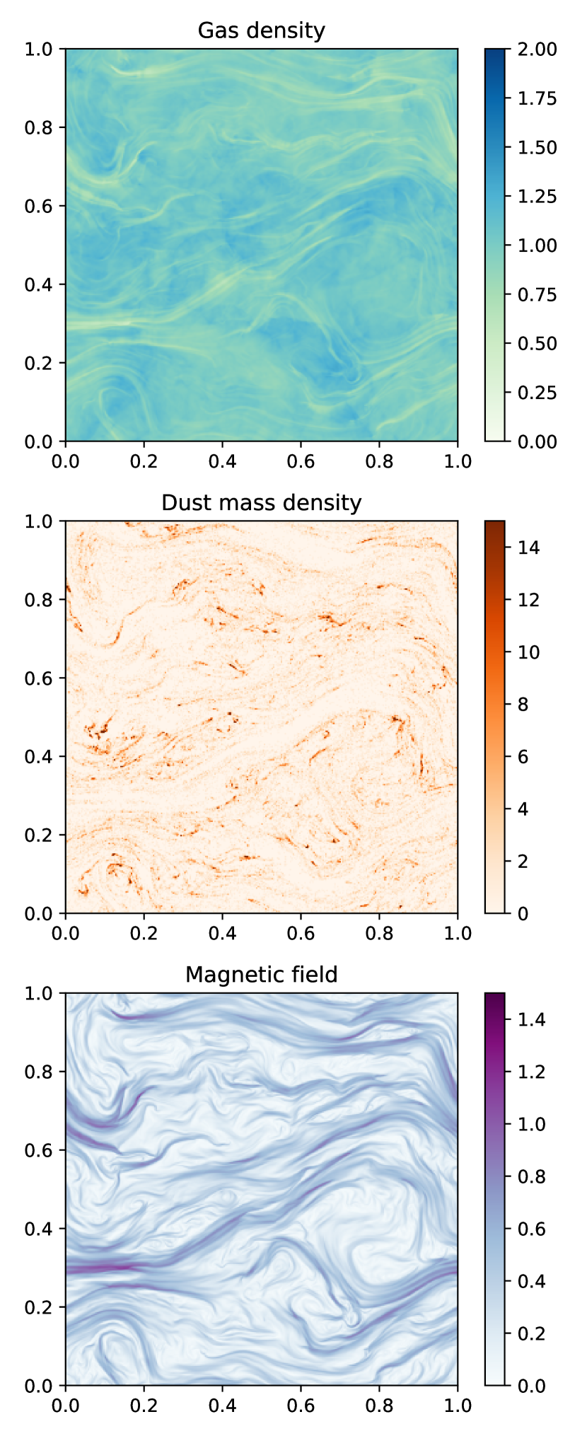
Figure 1: Upper panel: gas density map at the end of the simulation. It is normalized such that at t = 0, the density is constant and equal to 1. Middle panel: dust mass density map (see the text for the details of how it was built) for the same stage of the simulation. A dust mass value of 1 corresponds to the assumed dust-to-gas ratio of 0.01. Some clumps with larger values are observed all over the domain. Lower panel: magnetic field modulus, normalized such that at t = 0, it has a uniform value of $\sim 0.22$. Note the correlations between the dust and magnetic field structures.

If we look at the dust-to-gas ratio maps in Fig. 2, we observe that there are certain regions where the values are significantly larger than the initial average of 0.01 (value equal to unity in the normalized maps). On the other hand, there are some regions of the simulation where the dust-to-gas ratio is very small or that are completely devoid of dust. This is an expected result of the submission of charged dust to a spectrum of Alfvén waves. Finally, it is worth noting that the dust overdensities show a filamentary structure that will be studied in Sec. 3.3.

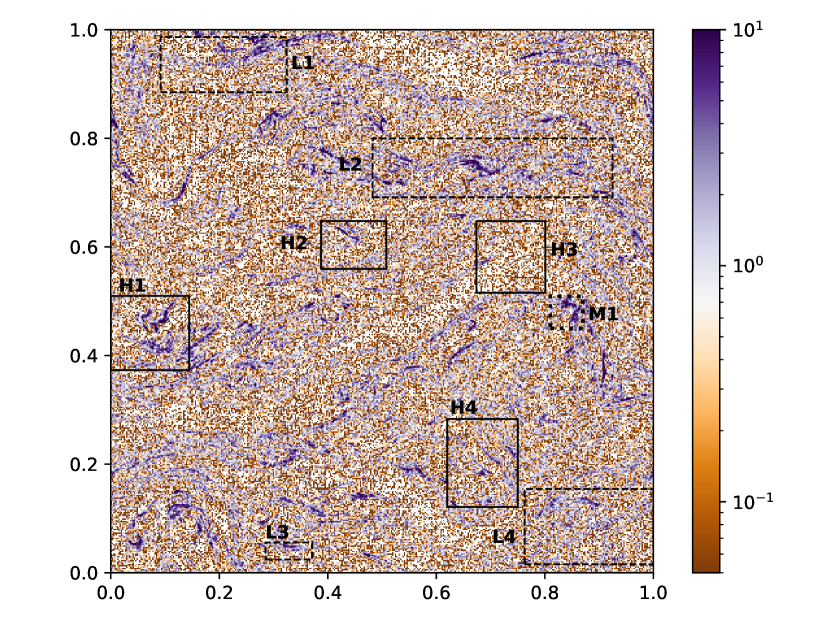
Figure 2: Dust-to-gas ratio map for the final stage of the simulation in log-scale. A value of 1 (0 in log scale, white colors) corresponds to the standard ratio of 0.01; larger values reveal regions where the dust density is dominant, while the regions with a value of 0 correspond to regions with a low or inexistent abundance of dust. Thick (dashed) rectangles encloses regions of high (low) gas density, and the small dotted region encloses an overdensity of dust that corresponds to a region of mid density.

The decoupling of gas and dust could arise due to the large differences between the particle stopping time $t_{s}$ and the Larmor time, $t_{L}=m_{d}c/|Z_{d}|e|\mathbf{B}|$. For all particles in the simulation at the final stage, the ratio $t_{s}/t_{L}$ is always greater than one (see Fig. 3) indicating that the coupling with the magnetic field is dominant. We selected some regions in the gas density map in order to study in detail the relationship between the distribution of dust, the gas density and the magnetic field strength. The regions are displayed in Fig. 2 and were selected such that a region of high (low) gas density shows values greater (lower) than $1\sigma$, since the gas distribution can be approximated by a Gaussian.

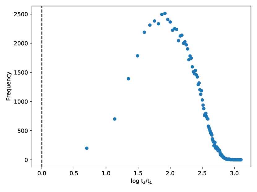
Figure 3: Histogram of the ratio $t_{s}/t_{L}$, particle stopping time over Larmor time (in logarithmic scale), for the final stage of the simulation. All particles show values greater than 0 ($t_{s}/t_{L}=1$, black dashed line), confirming the magnetic field coupling.

The analysis of the selected regions shown in Fig. 2 may be summarized as follows:

• At high gas density regions (Fig. 4) we observe large values of the dust-to-gas ratio forming filaments, parallel to the magnetic field.

• Except for region H3, where the dust density is extremely poor, the dust mean velocity is similar to the Alfvén velocity, pointing toward a strong coupling of dust with the magnetic field.

• At low gas density regions (Fig. 5), the dust filamentary structure is still observed, but there is more granulation and the filament widths are narrower. The modulus of the magnetic field in these regions is approximately 2.5 times greater than in regions H1-H4, and the dust velocity is again similar (and for regions L1 and L4 almost equal) to the Alfvén velocity.

• Finally, for the mid gas density region (Fig. 6) we observe a hybrid behavior. Dust filaments are also formed parallel to the magnetic field, but the overdensities are broader and, generally, perpendicular to the field. In this case, the mean dust motion seems more coupled to the gas dynamics.

Figure 4: Zoom of four high gas density regions labeled as H1-H4. On each panel, the left coloured map represents the normalized dust-to-gas ratio as in Fig. 2 with the magnetic field overlaid. Right panels represents the dust-to-gas velocity ratio.

Figure 5: Same as Fig. 4 but for low gas density regions.

Figure 6: Same as Fig. 4, but for a gas mid-density region.

3.3 Filamentary dust structure

In order to better understand the properties of the dust filaments generally decoupled from the gas (see Sec. 3.2), we analyzed in detail their properties using FilFinder (Koch & Rosolowsky, 2015) over the dust mass map at the final stage of the simulation. For the analysis, we created a custom mask preprocessing the map with the python packages scikit-image (van der Walt et al., 2014) and scikit-learn (Pedregosa et al., 2011). First, we binarized the map considering only pixels with a dust mass greater than the median; then, we identified connected regions and removed those with less than 10 pixels. The resulting mask is then passed as an argument to FilFinder together with the original dust map; we then skipped the flattening and creation of a mask steps and performed directly the identification and pruning of filaments; the results are shown in Fig. 7.

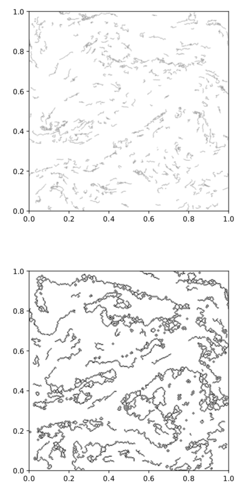
Figure 7: Dust filaments found by FilFinder for the original dust mass map (upper panel) and for a degraded version with one fourth of the resolution (lower panel). Short and numerous filaments are found for the original image, corresponding to the dense clumps. For the degraded image, longer branches tracing the general shape of the filaments are observed.

We found useful to study the filamentary structure over a degraded version of the map ($256\times 256$ px²) as well as over the original one ($1024\times 1024$ px²). While the latter represents well the fragmented structure of the dust clumps, the former gives an overall picture of the morphology of the dust filaments. The typical length of the filaments in the original image is 0.04 pc, while for the degraded image is 0.21 pc. We also computed the typical widths of the filaments as the mean width perpendicular to the longest path and found a value of 0.0035 pc for the high resolution image and 0.0087 pc for the degraded one; note that the image size imposes a resolution limit of $9.8\times 10^{-4}$ pc for the $1024\times 1024$ px² map, and of $3.9\times 10^{-3}$ pc for the $256\times 256$ px² one, but both mean widths are above that threshold. Table 1 summarizes all the parameters of the analyzed regions. It is evident that, although the resolution of the dust map critically affects the filament length, the widths are similar and an order of magnitude smaller than the typical width of 0.01 pc for gas filaments in molecular clouds found by Herschel (Arzoumanian et al. 2011 but see Panopoulou et al. 2017 for a recent discussion on the validity of such a characteristic width); since at large scales the correlation between dust and gas still holds, our results are in concordance with the observational report by Clark et al. (2014) on diffuse HI filaments at all resolved scales, up to a lower limit of 0.04 pc imposed by the instrumental resolution. However, the dust filament width should not depend on the resolution of the global simulation, because dust dynamics is resolved based on the gas properties on the adjacent cells. Hence, as dust grains are coupled to the magnetic field, an increase of the resolution only contributes to a better definition of the shape of the gas filaments, but the overall dynamics of dust grains should remain unchanged. What does affect the morphology of the dust filaments is the wave spectrum, as is discussed later in the following section. The dust structures will be more clumpy or filamentary depending on the propagating waves. In that sense, the box size may play a role since it sets an upper limit to the longest wavelength.

Table 1: Properties of the analyzed regions

Region	Dimensions	$<DGR>$	$<B>$	$<v_{A}>$	$<v_{gas}>$	$<v_{dust}>$	w1024	w256
	pc $\times$ pc		$10^{-6}$ G	$10^{5}$ cm s-1	$10^{5}$ cm s-1	$10^{5}$ cm s-1	$10^{-3}$ pc	$10^{-3}$ pc
H1	0.145 $\times$ 0.138	1.403	0.737	0.476	2.997	0.205	4.385	10.449
H2	0.121 $\times$ 0.089	0.798	0.829	0.534	2.402	0.135	2.981	9.975
H3	0.128 $\times$ 0.133	0.280	1.262	0.806	3.069	0.361	3.818	6.331
H4	0.131 $\times$ 0.163	1.090	1.015	0.649	2.629	0.558	4.109	9.827
L1	0.233 $\times$ 0.103	1.597	2.703	2.124	6.293	0.479	3.046	8.523
L2	0.443 $\times$ 0.109	1.767	2.437	1.841	5.935	0.597	3.300	11.728
L3	0.087 $\times$ 0.032	1.921	1.862	1.368	1.982	0.162	4.112	8.464
L4	0.238 $\times$ 0.140	1.459	2.514	1.910	5.010	0.280	3.362	10.919
M1	0.062 $\times$ 0.060	2.514	0.777	0.532	6.104	1.534	4.939	17.578

Note. — Mean quantities for the dust-to-gas ratio (denoted by $DGR$), magnetic field, Alfvén velocity, gas velocity, and dust velocity. Also included are the mean dust filament widths on each region for the original map (w₁₀₂₄) and for a degraded version (w₂₅₆).

We have also studied the mean dust-to-gas ratio along the longest paths of the filaments, and the results are shown in Fig. 8. We find that, in general, the ratio reaches values six times greater than the average value for the ISM and spans from $\sim 3$ to $\sim 17$, another indicative that dust filaments are not tightly correlated with gas filaments. However, if those mean values are normalized by the filament’s length (number of pixels, L_pix, Fig. 8, lower panel) one can see that the dust-to-gas ratio inside each filament is approximately constant and proportional to its length by a factor that oscilates between 0.1 and 0.3. There not seems to be any apparent relationship between the dust-to-gas ratio of a dust filament and its width, what suggests that such width may be characteristic of the dust filaments. However, to confirm that hypothesis, more realistic simulations that consider a whole representative dust population are needed.

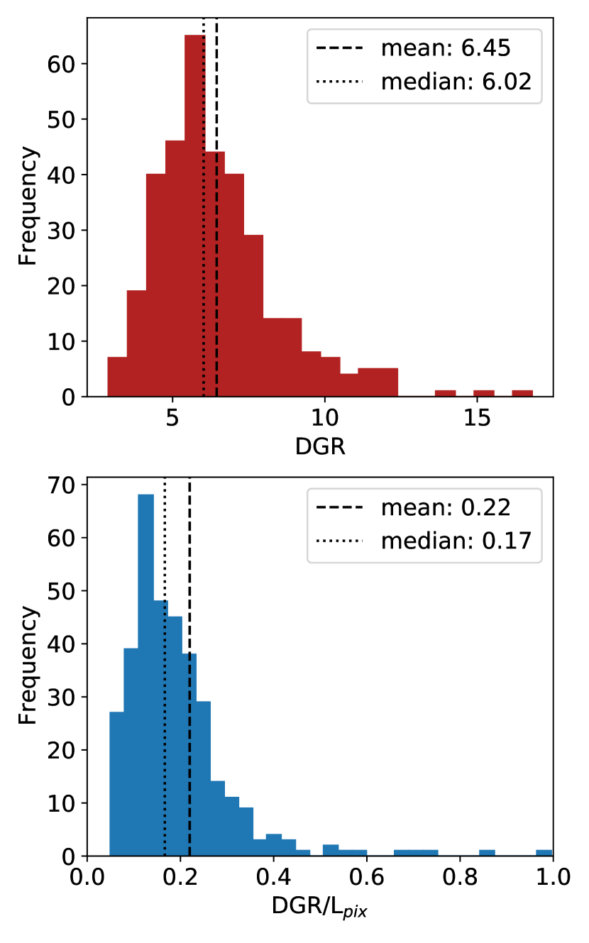
Figure 8: Upper panel: histogram of the dust-to-gas ratio along the filaments found by FilFinder over the original dust map. The values range between 3 and 17 times the typical ISM ratio (value of 1, see Fig. 2). Lower panel: dust-to-gas ratios normalized by their length in pixels, L_pix.

With respect to the relative orientation between the dust filaments and the magnetic field, we find that in general dust filaments tend to be aligned with the magnetic field, see Fig. 9; in the high-resolution map, $\sim 15$% of the filaments have relative orientations between $\pm 0.05$ rad (parallel), while the vast majority (98%) have relative angles inside the range $\pm\pi/4$ (dotted lines in Fig. 9). These angles have been computed along the skeleton of each dust filament as follows: every three pixels of the skeleton, the dot product between the magnetic field vector at the intermediate pixel and the skeleton vector is used to retrieve the relative angle between them, and is restricted to be inside the range $([-\pi/2,\pi/2))$.

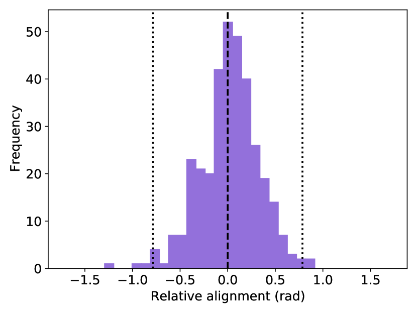
Figure 9: Histogram of relative alignment between the dust filaments and the magnetic field. The dashed vertical line is plotted at 0 rad (perfect parallel alignment) while the vertical dotted lines correspond to $\pm\pi/4$ rad.

4 Discussion

It is a common practice to assume a standard relationship between the dust and gas abundance. However, local variations of the dust-to-gas ratio are to be expected (Padoan et al., 2006; Hopkins, 2014), especially when the dust particles are charged (Lazarian & Yan, 2002; Lee et al., 2017), and they are actually found in the diffuse medium and even inside a cloud (Siebenmorgen et al., 2017; Chen et al., 2015; Reach et al., 2015). There were some early attempts to determine the scale of the fluctuations from extinction measurements (Thoraval et al., 1997, 1999) and variations of the dust size distribution have been found in MCs (Flagey et al., 2009; Köhler et al., 2015; Gómez de Castro et al., 2015; Beitia-Antero & Gómez de Castro, 2017). However, most of the studies are focused on the cool interiors of MCs since the main interest is to determine the possible influence of this phenomenon over the star formation processes. But if one aims to understand how dust may affect star formation and the formation of molecular clouds themselves, it is necessary to begin analyzing its behaviour in MC envelopes, where the coupling to the magnetic field favors the propagation of hydromagnetic waves into the cloud and increase the turbulent state of the molecular gas.

Despite the simplicity of our model and having considered an initial homogeneous distribution of dust and gas, we have shown that the propagation of velocity waves produce local variations of the dust-to-gas ratio, forming narrow dust filaments aligned with the magnetic field. Due to the random distribution of dust grains at the beginning of the simulation, the ratio is not constant even at the initial stage of the simulation, although the mean scarcely varies with time at large scales, as shown in Fig. 10. This fact could support the argument that, at large scales, the dust-to-gas ratio is nearly constant. However, at small scales there are appreciable deviations of the ratio that are far from a linear relationship. In Fig. 11, the histogram of the dust-to-gas ratio map presented in Fig. 2 is shown; there are clear variations of the ratio, and the peak of the distribution is far from the assumed dust-to-gas ratio (dashed vertical line).

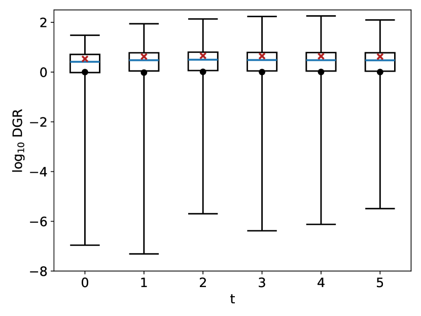
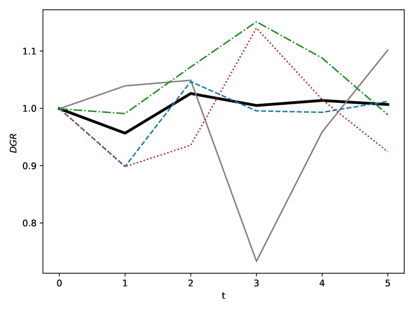
Figure 10: Time evolution of the dust-to-gas ratio, denoted by $DGR$. The upper panel shows, in logarithmic scale, a boxplot for dust-to-gas ratio values different from zero. The horizontal blue line limits the median, the mean is represented by a red cross, and the whiskers limits have been set to the maximum and minimum values. If null values in the map are considered, both the median and the first quantile are 0 (in linear scale); however, the mean represents well the assumed initial dust-to-gas ratio (black circles). The lower panel shows the variations of the mean ratio (black thick line) and the local variations when the whole simulation is analyzed in four large quadrants (gray solid line, blue dashed line, red dotted line, and green dotted dashed line). Note that the overall mean ratio is conserved although local variations are observed.

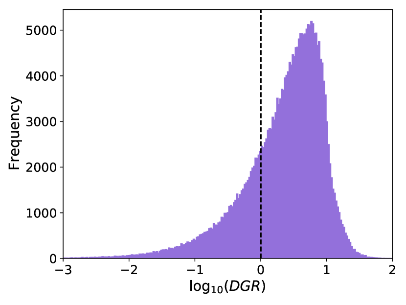
Figure 11: Histogram of the dust-to-gas ratio map shown in Fig. 2. Values greater than 1 (0 in the logscale, vertical dashed line) indicate a dust density value above the expected one. This plot highlights the fact that values ten times greater than the expected for the standard ratio of the diffuse ISM are common in the simulation, and that the relationship between gas and dust densities is far from being linear.

Recently, Lee et al. (2017) reported deviations of the dust-to-gas ratio in the cold neutral medium and Hopkins & Squire (2018) studied in detail the spectrum of instabilities that may arise when charged dust moves in a magnetized gas. In particular, they report that for the WNM the relative velocity between dust particles and gas should be subsonic and that the dominant resonances tend to form structures parallel to the magnetic field. Our results are compatible up to a point, since the majority of the structures are indeed aligned with the magnetic field and the mean dust and gas velocities differ a few tens of km s^-1, see Table 1. These results are also in good agreement with observational evidence of dust filaments with low column densities aligned with the magnetic field (Planck Collaboration et al., 2016; Fissel et al., 2019). There seems to be only an exception with the mid-density region (see Fig. 6), where a dust structure is formed perpendicular to the magnetic field direction. We attribute this localized phenomenon to the clear decrease of the magnetic field strength along the structure.

Additionally, we studied separately the influence of the largest and shortest waves of the initial velocity spectrum in the formation of dust structures. As can be seen in Fig. 12, the shortest wave does not inject enough energy to the medium to produce conspicuous filamentary structures. Nevertheless, tiny clumps of a few ($\leq 10$) pixels are formed, and the histogram of the dust-to-gas ratio is very similar to the one for the complete simulation shown in Fig. 11. For the longest wave, the energy input is so strong that relevant fluctuations are appreciable in density, momentum, and magnetic field distributions. These variations enable the formation of dust filaments with a dust-to-gas ratio distribution that again resembles to the one in Fig. 11. We draw two conclusions from this analysis: first, that variations in the dust-to-gas ratio are expected to arise whenever a wave propagates in a molecular cloud envelope, no matter the energy of the wave; and second, that the morphology of the structures that can be formed in such a medium depends on the wave spectrum. It is of interest to explore in a future work if other properties of the dust filaments, such as their widths, depend on the wave spectrum or if they have a characteristic size. Finally, we want to highlight again that the choice of the box size sets an upper limit to the longest wavelength that we are able to resolve ($L_{0}$), so we are always talking about stuctures at scales lower than $L_{0}=1$ pc.

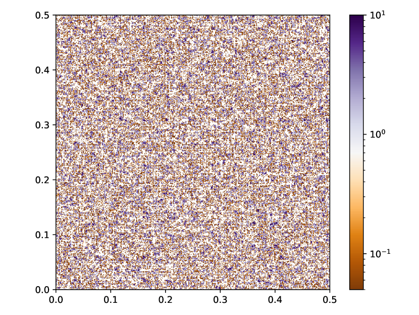
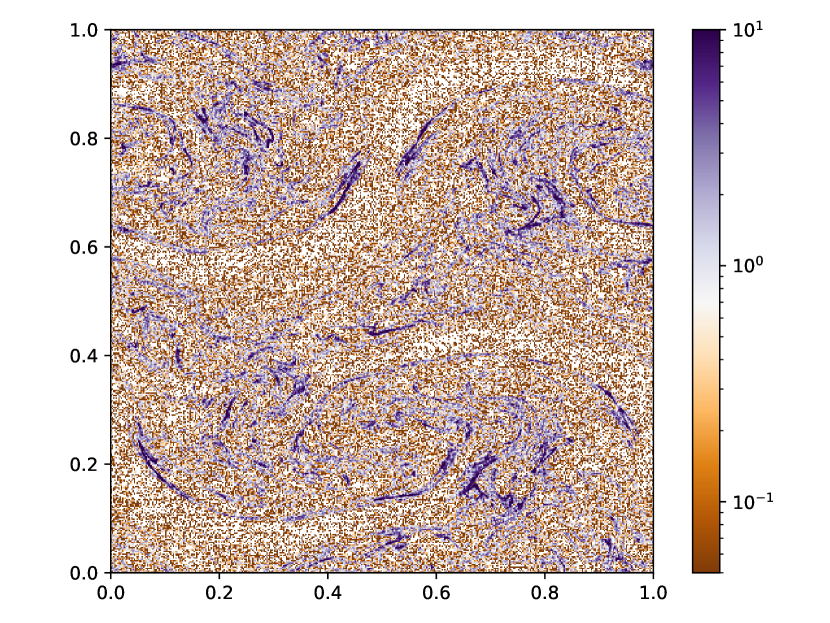
Figure 12: Dust-to-gas maps for single wave evolution at the final stage of the simulation. The upper panel corresponds to the shortest wavelength ($\lambda=1/24$) and the simulation has been run in a domain half the size of the original to optimize the computational resources. The lower panel corresponds to the longest wavelength ($\lambda=1$). These plots show that the shortest wavelengths by themselves can only produce a clumpy distribution with localized overdensities, while the longest ones define the filamentary structures.

4.1 Limitations of the model

There are some points to be taken into account when comparing these results with observations. Some of them are related to the necessary simplifications incorporated in the current model, and others are linked to the typical plasma conditions of the MC envelopes that we have modelled.

The first point is that our model is 2D. This implies that the motion of the particles is produced by polarized Alfvén waves. In 3D, the stirring of the plasma will be in 3D and the filaments too. Adding a degree of freedom will likely result in shorter, helical filaments..

The second point is that we have only evolved a single population of dust with fixed radius, while in the diffuse ISM a realistic size distribution that evolves with time should be considered. With that purpose, we have developed an additional module for Athena to follow dust coagulation and shattering that will be presented in a forthcoming paper (Beitia-Antero et al. in prep.).

And finally, the relevance of resistive processes, and ambipolar and Hall diffusion should be taken into account. The impact of these effects will be studied in subsequent works.

It is also relevant to highlight that the modeled phase is very diffuse, partially ionised, and the dust particles are very small ($a_{d}=0.05~{}\mu$m) so it is better traced by UV and optical tracers rather than with infrared/submillimeter ones. Observations of MC envelopes with high sensitivity, wide field, UV imagers will provide invaluable results for this research.

5 Conclusions

In this work, we have described a new module developed for Athena to deal with the interaction of charged dust particles in astronomical magnetized fluids. The code is applied to the study of dust dynamics in diffuse molecular cloud envelopes, and its performance is illustrated through the formation of dust filaments decoupled from the gas. The model for a molecular cloud envelope considers a density of $n=10$ cm^-3, with a temperature of $T=6000$ K and an ionization fraction $\chi=0.1$, and includes a single population of charged dust silicate particles of radius $0.05~{}\mu$m.

We show that charged dust grains follow the magnetic field and form filamentary structures with a typical width of 0.0035-0.0087 pc. Although the mean dust-to-gas ratio is globally preserved, local variations are observed that are not always correlated with gas density; these variations are in concordance with previous theoretical (Padoan et al., 2006; Hopkins, 2014) and observational (Siebenmorgen et al., 2017; Chen et al., 2015; Reach et al., 2015) results.

Although a more realistic model (non-ideal MHD effects and a full dust distribution) is needed, our results highlight the importance of considering the dynamics of charged dust for star formation studies even at a low-density regime characteristic of a molecular cloud envelope.

Appendix A Code tests

We designed two very simple tests to check that the movement of charged particles is correctly solved in 2D. Both tests consider a positively charged grain, initially at rest, embedded in a uniform medium moving at constant speed parallel to the x-axis. The constant magnetic field is parallel to the z-axis, perpendicular to the domain we are solving.

A.1 Lorentz force term

The first test is intended to check the integration accuracy of the Lorentz force term. The problem to be solved analytically is:

$$\frac{d{\bf x}}{dt}={\bf v},~{}~{}{\bf x}(0)=(x_{0},x_{1})$$

$$\frac{d{\bf v}}{dt}=-\frac{{\bf v}-{\bf u}}{t_{s}}+Q({\bf v}-{\bf u})\times{\bf B},~{}~{}{\bf v}(0)=(0,0)$$

Depending on the ratio between $t_{s}$ and $Q|\mathbf{B}|\doteq QB$, the particle motion will be dominated by gas drag ($t_{s}^{-1}\gg QB$) or by magnetic effects ($t_{s}^{-1}\ll QB$). Hence, we run four tests up to $t=10t_{s}$ for a fiducial stopping time $t_{s}=1$ and have considered the following values for the pair $(Q,B)$: test A (0.1, 0.1), test B (0.1, 1), test C (0.1, 10), and test D (1, 10). For all the cases (see Fig. 13) the error in position is of the order of $10^{-3}$ or lower, and the error in velocity is at most of the order of $10^{-2}$, which confirms that our integrator for the Lorentz term works well and preserves the second-order accuracy. We want to note that for a magnetic-dominated medium ($QB\sim 100$) it is necessary to diminish even more the timestep in Eq. 6 because with the current implementation, the integration diverges after a few timesteps. However, for studies of dust in the interstellar medium such harsh conditions are not expected, so the implementation of the integrator presented here is adequate for our purposes.

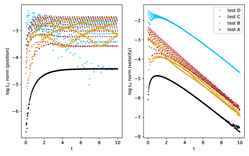
Figure 13: L2 norm for position (left) and velocity (right) for the test of the Lorentz force term and a CFL = 0.8. Black triangles correspond to test A, for which the aerodynamic drag is dominant. For tests B (orange squares), C (red updown triangles), and D (blue circles), the magnetic effects become increasingly dominant and oscillations in the errors are appreciable; however, they are always of the order of $10^{-3}$ or better for position, and $10^{-2}$ or better for velocity.

A.2 Coulomb drag

This test is defined to test the Coulomb drag term in the full Eq. 1. We run test D ($Q=1$, $B=10$) for $\nu=0.1,1,10$ to study how it effects the transition from the aerodynamic regime to the magnetic one; the results are shown in Fig. 14 The main effect of the electric drag is the damping of the magnetic oscillation of the charged grain, that can be rapidly supressed for large values of $\nu$; however, it will be typically lower than $Q$ since $\nu\propto Q^{2}$ (Eq. 2). This implies that the overall accuracy of the integrator is kept second-order, since the oscillations in the precision arise from the effects of the Lorentz force.

Figure 14: Results for the test of the Coulomb electric drag of a positively charged grain in the presence of a gas moving uniformly in the x-direction and a magnetic field oriented parallel to the z-axis. Position (upper left) and velocity (lower left) diagrams are shown for $\nu=0.1$ (black dashed line), $\nu=1$ (blue dashed-dotted line), and $\nu=10$ (red dotted line); the thick light gray curve shows the dynamics of the charged particle without considering the Coulomb drag. $L_{2}$ norm of the errors in position (upper right) and velocity (lower right) are also shown.

References

- André et al. (2010) André, P., Men’shchikov, A., Bontemps, S., et al. 2010, A&A, 518, L102, doi: 10.1051/0004-6361/201014666
- Arzoumanian et al. (2011) Arzoumanian, D., André, P., Didelon, P., et al. 2011, A&A, 529, L6, doi: 10.1051/0004-6361/201116596
- Bacchini et al. (2020) Bacchini, C., Fraternali, F., Iorio, G., et al. 2020, arXiv e-prints, arXiv:2006.10764. https://arxiv.org/abs/2006.10764
- Bai & Stone (2010) Bai, X.-N., & Stone, J. M. 2010, ApJS, 190, 297, doi: 10.1088/0067-0049/190/2/297
- Bakes & Tielens (1994) Bakes, E. L. O., & Tielens, A. G. G. M. 1994, ApJ, 427, 822, doi: 10.1086/174188
- Ballesteros-Paredes et al. (2020) Ballesteros-Paredes, J., André, P., Hennebelle, P., et al. 2020, Space Sci. Rev., 216, 76, doi: 10.1007/s11214-020-00698-3
- Balsara (1996) Balsara, D. S. 1996, ApJ, 465, 775, doi: 10.1086/177462
- Beitia-Antero & Gómez de Castro (2017) Beitia-Antero, L., & Gómez de Castro, A. I. 2017, MNRAS, 469, 2531, doi: 10.1093/mnras/stx881
- Blitz et al. (2007) Blitz, L., Fukui, Y., Kawamura, A., et al. 2007, in Protostars and Planets V, ed. B. Reipurth, D. Jewitt, & K. Keil, 81. https://arxiv.org/abs/astro-ph/0602600
- Bohlin et al. (1978) Bohlin, R. C., Savage, B. D., & Drake, J. F. 1978, ApJ, 224, 132, doi: 10.1086/156357
- Boris (1970) Boris, J. 1970, in Proc. Fourth Conf. on Numerical Simulation of Plasmas (Washington, DC: Naval Research Lab), 3
- Boulanger et al. (1996) Boulanger, F., Abergel, A., Bernard, J. P., et al. 1996, A&A, 312, 256
- Cazaux & Tielens (2004) Cazaux, S., & Tielens, A. G. G. M. 2004, ApJ, 604, 222, doi: 10.1086/381775
- Chapman & Wardle (2006) Chapman, J. F., & Wardle, M. 2006, MNRAS, 371, 513, doi: 10.1111/j.1365-2966.2006.10592.x
- Chen et al. (2015) Chen, B. Q., Liu, X. W., Yuan, H. B., Huang, Y., & Xiang, M. S. 2015, MNRAS, 448, 2187, doi: 10.1093/mnras/stv103
- Chevance et al. (2020) Chevance, M., Kruijssen, J. M. D., Vazquez-Semadeni, E., et al. 2020, Space Sci. Rev., 216, 50, doi: 10.1007/s11214-020-00674-x
- Clark et al. (2014) Clark, S. E., Peek, J. E. G., & Putman, M. E. 2014, ApJ, 789, 82, doi: 10.1088/0004-637X/789/1/82
- Cramer & Vladimirov (1997) Cramer, N. F., & Vladimirov, S. V. 1997, PASA, 14, 170, doi: 10.1071/AS97170
- Elmegreen & Scalo (2004) Elmegreen, B. G., & Scalo, J. 2004, ARA&A, 42, 211, doi: 10.1146/annurev.astro.41.011802.094859
- Falceta-Gonçalves et al. (2003) Falceta-Gonçalves, D., de Juli, M. C., & Jatenco-Pereira, V. 2003, ApJ, 597, 970, doi: 10.1086/378584
- Falgarone & Phillips (1996) Falgarone, E., & Phillips, T. G. 1996, ApJ, 472, 191, doi: 10.1086/178054
- Falgarone et al. (2005) Falgarone, E., Verstraete, L., Pineau Des Forêts, G., & Hily-Blant, P. 2005, A&A, 433, 997, doi: 10.1051/0004-6361:20041893
- Federrath (2015) Federrath, C. 2015, MNRAS, 450, 4035, doi: 10.1093/mnras/stv941
- Ferrière (2001) Ferrière, K. M. 2001, Reviews of Modern Physics, 73, 1031, doi: 10.1103/RevModPhys.73.1031
- Fiege & Pudritz (2000) Fiege, J. D., & Pudritz, R. E. 2000, MNRAS, 311, 105, doi: 10.1046/j.1365-8711.2000.03067.x
- Fissel et al. (2019) Fissel, L. M., Ade, P. A. R., Angilè, F. E., et al. 2019, ApJ, 878, 110, doi: 10.3847/1538-4357/ab1eb0
- Flagey et al. (2009) Flagey, N., Noriega-Crespo, A., Boulanger, F., et al. 2009, ApJ, 701, 1450, doi: 10.1088/0004-637X/701/2/1450
- Fukui et al. (2017) Fukui, Y., Tsuge, K., Sano, H., et al. 2017, PASJ, 69, L5, doi: 10.1093/pasj/psx032
- Fukui et al. (2009) Fukui, Y., Kawamura, A., Wong, T., et al. 2009, ApJ, 705, 144, doi: 10.1088/0004-637X/705/1/144
- Gómez de Castro et al. (2015) Gómez de Castro, A. I., López-Santiago, J., López-Martínez, F., et al. 2015, MNRAS, 449, 3867, doi: 10.1093/mnras/stv413
- Hocuk & Spaans (2010) Hocuk, S., & Spaans, M. 2010, A&A, 510, A110, doi: 10.1051/0004-6361/200912236
- Hollenbach & Salpeter (1971) Hollenbach, D., & Salpeter, E. E. 1971, ApJ, 163, 155, doi: 10.1086/150754
- Hopkins (2014) Hopkins, P. F. 2014, ApJ, 797, 59, doi: 10.1088/0004-637X/797/1/59
- Hopkins & Squire (2018) Hopkins, P. F., & Squire, J. 2018, MNRAS, 479, 4681, doi: 10.1093/mnras/sty1604
- Hopkins et al. (2020) Hopkins, P. F., Squire, J., & Seligman, D. 2020, MNRAS, 496, 2123, doi: 10.1093/mnras/staa1046
- Inutsuka et al. (2015) Inutsuka, S.-i., Inoue, T., Iwasaki, K., & Hosokawa, T. 2015, A&A, 580, A49, doi: 10.1051/0004-6361/201425584
- Ivlev et al. (2018) Ivlev, A. V., Dogiel, V. A., Chernyshov, D. O., et al. 2018, ApJ, 855, 23, doi: 10.3847/1538-4357/aaadb9
- Ivlev et al. (2015) Ivlev, A. V., Padovani, M., Galli, D., & Caselli, P. 2015, ApJ, 812, 135, doi: 10.1088/0004-637X/812/2/135
- Klessen & Glover (2016) Klessen, R. S., & Glover, S. C. O. 2016, Saas-Fee Advanced Course, 43, 85, doi: 10.1007/978-3-662-47890-5_2
- Koch & Rosolowsky (2015) Koch, E. W., & Rosolowsky, E. W. 2015, MNRAS, 452, 3435, doi: 10.1093/mnras/stv1521
- Köhler et al. (2015) Köhler, M., Ysard, N., & Jones, A. P. 2015, A&A, 579, A15, doi: 10.1051/0004-6361/201525646
- Kruijssen et al. (2019) Kruijssen, J. M. D., Dale, J. E., Longmore, S. N., et al. 2019, MNRAS, 484, 5734, doi: 10.1093/mnras/stz381
- Lallement et al. (2003) Lallement, R., Welsh, B. Y., Vergely, J. L., Crifo, F., & Sfeir, D. 2003, A&A, 411, 447, doi: 10.1051/0004-6361:20031214
- Lazarian & Yan (2002) Lazarian, A., & Yan, H. 2002, ApJ, 566, L105, doi: 10.1086/339675
- Lee et al. (2017) Lee, H., Hopkins, P. F., & Squire, J. 2017, MNRAS, 469, 3532, doi: 10.1093/mnras/stx1097
- Lehe et al. (2009) Lehe, R., Parrish, I. J., & Quataert, E. 2009, ApJ, 707, 404, doi: 10.1088/0004-637X/707/1/404
- Lenz et al. (2017) Lenz, D., Hensley, B. S., & Doré, O. 2017, ApJ, 846, 38, doi: 10.3847/1538-4357/aa84af
- Martin et al. (2015) Martin, P. G., Blagrave, K. P. M., Lockman, F. J., et al. 2015, ApJ, 809, 153, doi: 10.1088/0004-637X/809/2/153
- Mathis et al. (1983) Mathis, J. S., Mezger, P. G., & Panagia, N. 1983, A&A, 500, 259
- Meidt et al. (2018) Meidt, S. E., Leroy, A. K., Rosolowsky, E., et al. 2018, ApJ, 854, 100, doi: 10.3847/1538-4357/aaa290
- Mignone et al. (2019) Mignone, A., Flock, M., & Vaidya, B. 2019, ApJS, 244, 38, doi: 10.3847/1538-4365/ab4356
- Myers & Goodman (1988) Myers, P. C., & Goodman, A. A. 1988, ApJ, 329, 392, doi: 10.1086/166385
- Nakamura & Li (2008) Nakamura, F., & Li, Z.-Y. 2008, ApJ, 687, 354, doi: 10.1086/591641
- Nakano (1998) Nakano, T. 1998, ApJ, 494, 587, doi: 10.1086/305230
- Offner & Liu (2018) Offner, S. S. R., & Liu, Y. 2018, Nature Astronomy, 2, 896, doi: 10.1038/s41550-018-0566-1
- Padoan et al. (2006) Padoan, P., Cambrésy, L., Juvela, M., et al. 2006, ApJ, 649, 807, doi: 10.1086/507068
- Padoan et al. (2016) Padoan, P., Pan, L., Haugbølle, T., & Nordlund, Å. 2016, ApJ, 822, 11, doi: 10.3847/0004-637X/822/1/11
- Palmeirim et al. (2013) Palmeirim, P., André, P., Kirk, J., et al. 2013, A&A, 550, A38, doi: 10.1051/0004-6361/201220500
- Pandey & Vladimirov (2019) Pandey, B. P., & Vladimirov, S. V. 2019, AJ, 157, 83, doi: 10.3847/1538-3881/aafc32
- Panopoulou et al. (2017) Panopoulou, G. V., Psaradaki, I., Skalidis, R., Tassis, K., & Andrews, J. J. 2017, MNRAS, 466, 2529, doi: 10.1093/mnras/stw3060
- Pedregosa et al. (2011) Pedregosa, F., Varoquaux, G., Gramfort, A., et al. 2011, Journal of Machine Learning Research, 12, 2825
- Pilipp et al. (1987) Pilipp, W., Hartquist, T. W., Havnes, O., & Morfill, G. E. 1987, ApJ, 314, 341, doi: 10.1086/165064
- Pinto et al. (2008) Pinto, C., Galli, D., & Bacciotti, F. 2008, A&A, 484, 1, doi: 10.1051/0004-6361:20078818
- Planck Collaboration et al. (2016) Planck Collaboration, Adam, R., Ade, P. A. R., et al. 2016, A&A, 586, A135, doi: 10.1051/0004-6361/201425044
- Planck Collaboration et al. (2018a) Planck Collaboration, Akrami, Y., Ashdown, M., et al. 2018a, arXiv e-prints, arXiv:1801.04945. https://arxiv.org/abs/1801.04945
- Planck Collaboration et al. (2018b) Planck Collaboration, Aghanim, N., Akrami, Y., et al. 2018b, arXiv e-prints, arXiv:1807.06212. https://arxiv.org/abs/1807.06212
- Predehl & Schmitt (1995) Predehl, P., & Schmitt, J. H. M. M. 1995, A&A, 500, 459
- Price et al. (2018) Price, D. J., Wurster, J., Tricco, T. S., et al. 2018, PASA, 35, e031, doi: 10.1017/pasa.2018.25
- Reach et al. (2015) Reach, W. T., Heiles, C., & Bernard, J.-P. 2015, ApJ, 811, 118, doi: 10.1088/0004-637X/811/2/118
- Redfield et al. (2004) Redfield, S., Wood, B. E., & Linsky, J. L. 2004, Advances in Space Research, 34, 41, doi: 10.1016/j.asr.2003.02.053
- Roman-Duval et al. (2010) Roman-Duval, J., Israel, F. P., Bolatto, A., et al. 2010, A&A, 518, L74, doi: 10.1051/0004-6361/201014575
- Savage et al. (1977) Savage, B. D., Bohlin, R. C., Drake, J. F., & Budich, W. 1977, ApJ, 216, 291, doi: 10.1086/155471
- Savage & Sembach (1991) Savage, B. D., & Sembach, K. R. 1991, ApJ, 379, 245, doi: 10.1086/170498
- Seligman et al. (2019) Seligman, D., Hopkins, P. F., & Squire, J. 2019, MNRAS, 485, 3991, doi: 10.1093/mnras/stz666
- Shingledecker et al. (2020) Shingledecker, C. N., Lamberts, T., Laas, J. C., et al. 2020, ApJ, 888, 52, doi: 10.3847/1538-4357/ab5360
- Siebenmorgen et al. (2017) Siebenmorgen, R., Voschinnikov, N., Bagnulo, S., Cox, N., & Cami, J. 2017, in Submm/mm/cm QUESO Workshop 2017 (QUESO2017), 27, doi: 10.5281/zenodo.1038101
- Spitzer (1954) Spitzer, Lyman, J. 1954, ApJ, 120, 1, doi: 10.1086/145876
- Stone et al. (2008) Stone, J. M., Gardiner, T. A., Teuben, P., Hawley, J. F., & Simon, J. B. 2008, ApJS, 178, 137, doi: 10.1086/588755
- Thoraval et al. (1997) Thoraval, S., Boisse, P., & Duvert, G. 1997, A&A, 319, 948
- Thoraval et al. (1999) Thoraval, S., Boissé, P., & Duvert, G. 1999, A&A, 351, 1051
- van der Walt et al. (2014) van der Walt, S., Schönberger, J. L., Nunez-Iglesias, J., et al. 2014, PeerJ, 2, e453, doi: 10.7717/peerj.453
- Wardle (2007) Wardle, M. 2007, Ap&SS, 311, 35, doi: 10.1007/s10509-007-9575-8
- Weidenschilling (1977) Weidenschilling, S. J. 1977, MNRAS, 180, 57, doi: 10.1093/mnras/180.1.57
- Weingartner & Draine (2001) Weingartner, J. C., & Draine, B. T. 2001, ApJS, 134, 263, doi: 10.1086/320852
- Welsh et al. (2010) Welsh, B. Y., Lallement, R., Vergely, J. L., & Raimond, S. 2010, A&A, 510, A54, doi: 10.1051/0004-6361/200913202
- Wolfire et al. (1995) Wolfire, M. G., Hollenbach, D., McKee, C. F., Tielens, A. G. G. M., & Bakes, E. L. O. 1995, ApJ, 443, 152, doi: 10.1086/175510