Puzzle-AE: Novelty Detection in Images through Solving Puzzles

Abstract

As an essential part of many anomaly detection methods, the autoencoder lacks flexibility on normal data in complex datasets. U-Net is proven effective for this purpose but overfits the training data if trained only using reconstruction error similar to other AE-based frameworks. As a pretext task of self-supervised learning (SSL) methods, Puzzle-solving has earlier proved its ability in learning semantically meaningful features. We show that training U-Nets based on this task effectively prevents overfitting and facilitates learning beyond pixel-level features. Shortcut solutions, however, are a big challenge in SSL tasks, including jigsaw puzzles. We propose robust adversarial training as an effective automatic shortcut removal. We achieve competitive or superior results compared to the State of the Art (SOTA) anomaly detection methods on various toy and real-world datasets. Unlike many competitors, the proposed framework is stable, fast, data-efficient, and does not require unprincipled early stopping.

1 Introduction

Anomaly/novelty is defined as any digression from the essential features of any given phenomenon. The main task of novelty detection is to infer deviated features from extracted normal training samples’ features. For instance, having a model trained on healthy brain ct-scan images, it should be able to find non-healthy test input images by comparing current extracted features, and the expected ones with different metrics [1, 2, 3].

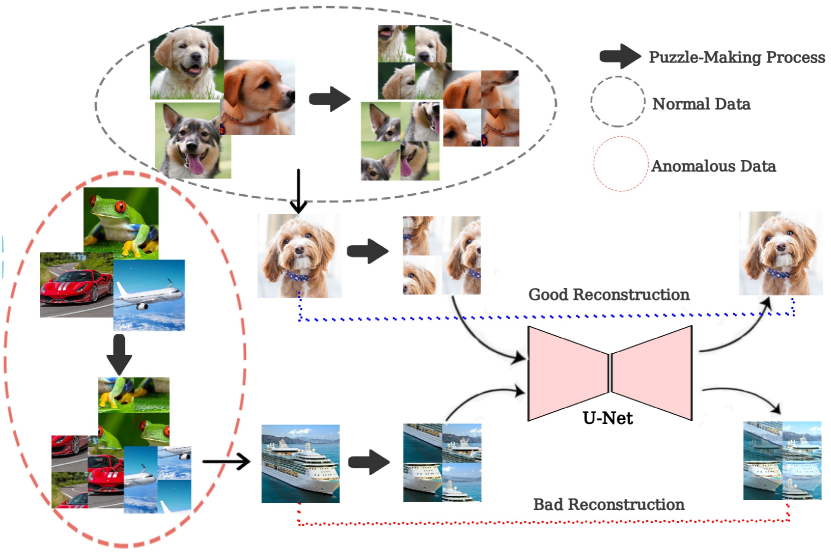
Figure 1: Reconstruction of normal and anomalous inputs during the testing phase. As it is shown, the model is unable to solve the puzzle for anomalous inputs, which do not have the main features existing in the normal data. As a result, anomalous samples produce high reconstruction loss, whereas normal inputs have low reconstruction loss since their puzzles are perfectly solved by the model.

Although Area Under the Curve (AUC) has been used as the primary distinctive metric between binary classifiers’ performances, this criterion is not sufficient alone. That is because AUC shows the average performance of a model in different operating points. However, a fixed operating point of the Receiver Operating Characteristic (ROC) curve is needed in many practical applications, which is usually when True Positive Rate (TPR) is equal to 0.99 or 0.995. In some applications, such as medical and industrial defect detections, data efficiency and real-time performance are key factors for practicality [1, 4]. Another practical criterion is the adaptability of a given framework to other datasets. For example, we generally require the model to be agnostic to various hyperparameters’ choices and have access to well-known criteria to determine when to stop training of the model. In this paper, we propose a new framework and compare its practicality with the SOTA approaches concerning the mentioned criteria. Our results show this framework performs well under all these criteria.

In the literature, GAN based methods [5],[6] suffer from non-reproducibility of the results [7],[8] and data hungriness. Likewise, autoregressive approaches have significantly poor performance [9]. Moreover, we show that one-class methods such as DSVDD [10] suffer from converging to trivial solutions and need confronting techniques such as early stopping that is not easy to find due to the one-class formulation of the problem. These all cause the generality and impracticality problem.

On the other hand, AE-based methods often have a straightforward training process and yield reproducible results. It has been observed that an Autoencoder (AE) that is trained on just normal samples can reconstruct the normal test inputs while failing to reconstruct anomalous test samples [11]. However, various kinds of AEs have the issue of low-quality input reconstruction on complex datasets such as CIFAR-10 [12]. The reason for this phenomenon should be investigated in the training procedure of AE, which tries to model pixel intensities with a complex function that is represented by the decoder and leads to finding fallacious relationships between unnecessary or irrelevant features.

More recently, self-supervised learning methods have shown great potential to go beyond pixel-level and learn semantically meaningful features. Impressive unsupervised classification accuracy on the ImageNet [13] dataset in [14],[15],[16] has attracted a lot of attention to this field. GT [17] has introduced the first one-class classification method that utilizes self-supervised learning with great performance on the CIFAR-10 dataset [12]. However, we show that their performance is not even as good as the base AE on real-world datasets such as MVTecAD [18] and Medical images [19, 20].

We show that one way to benefit from all the significant aspects of AEs and alleviate their deficiencies is using U-Net [21] as a highly expressive AE-based model mixed with a well-defined and unambitious SSL pretext task. That is because U-Net has shown its ability in high-resolution image tasks such as segmentation [22, 23]. However, it could easily overfit when used similar to previous AE based methods such as denoising, etc. One excellent SSL pretext task that solves the overfitting problem and has a minor effect on the data agnosticism of AEs, since it keeps almost all the input information, is a puzzle-solving task [24, 25]. Training a U-Net to solve 4-part puzzled inputs like Fig. 1, would preserve good abilities of AEs while learning how to model normal input data in patch-level rather than pixel one.

However, according to [24], puzzles could be solved easily by finding low-level statistic shortcuts such as edge positions or patches’ mean and variance. Instead of using traditional approaches such as manual jittering, adversarial robust training [26, 27] as an automatic shortcut removal is used to make the shortcuts out of access for the U-Net, which enhances semantical abstraction modeling. Finally, having trained the framework in a GAN-based setting by considering the U-Net as the generator and adding a discriminator, we could increase the quality of generated images even more [28].

Our framework shows great performance on a large number of datasets. To the best of our knowledge, our work is the first study that produces a framework without any need to design unprincipled early stopping criterion while producing stable and reproducible results. Our main contribution is to provide solutions for the following issues:

1. High-quality normal sample reconstruction: Significantly improving the AE flexibility to better reconstruct the normal samples in complex real-world datasets. This is achieved by learning beyond pixel-level abstraction using self-supervised training, removing some of the shortcut features by robust adversarial training, and improving the quality of generated images by training the whole framework similar to the Generative Adversarial Network (GAN).

2. Method Stability: The generative nature of our proposed self-supervised method helps in reaching a stable model across the training epochs. We empirically notice the lack of this property in the earlier self-supervised frameworks for anomaly detection.

3. Shortcuts in the Jigsaw: Relieving the shortcut problem of the jigsaw puzzle pretext task automatically by robust adversarial training (which is traditionally solved by manual jittering).

4. Method Evaluation: Introducing new practical criteria, False Positive Rate (FPR) at a high TPR, and robustness to the test-time adversarial attacks that have not been tested on any recent SOTA models.

5. Method Generality: Competitive or better than SOTA performance on a wide range of problems without any need of unprincipled early stopping, and with a stable training process, yielding robust and reproducible results.

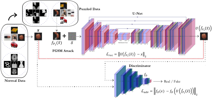
Figure 2: Anomaly Detection framework. As it illustrates, puzzled inputs are added to an FGSM noise to prevent shortcut detection. Then they are given to the U-Net to be solved. The whole framework is trained similar to GAN to improve the quality of reconstructed images.

2 Related Works

The major approaches to novelty detection are AE-based and one-class classification methods. Latent space autoregression (LSA) [29] is a popular AE-based method, which fits an autoregressive model to the AE bottleneck layer. By jointly training an autoregressive and AE model, it can learn a compact latent space for the normal samples. Hence, anomalous samples would have high reconstruction errors, but the value of their bottleneck layer would have a lower probability than the normal ones. This probability is called the “surprise score” in LSA. At testing time, the surprise score is added to the mean reconstruction error, and the sum is then thresholded to determine the class of a given sample.

OCGAN [30] uses an AE that is jointly trained with the reconstruction and generative adversarial error losses. In contrast to the LSA, it tries to force the encoder output distribution to be approximately uniform. This causes the decoder to reconstruct just normal outputs for normal and anomalous inputs, resulting in a higher mean squared error for abnormal input datum.

MemAE [4] is the first AE framework that uses memory in a non-parametric approach for novelty detection. When an input is passed to the AE, it is searched within the memory to find embeddings that match the input. Then, based on the combination of these embeddings, a new one is made and passed through the decoder.

Deep SVDD [10] is a one-class classification method that tries to convert data from the original space to the desired space by using deep neural networks. During the training process, it tries to put normal datum in a circle with a predefined center in a new space and then iteratively reduces its diameter. Because of the problem of finding trivial solutions, it uses early stopping and utilizes some constraints on the activation functions of layers. Geometric Transformations (GT) [17] is another one-class classification method that uses self-supervised learning. It makes a set of different transformations on the training data. Using a classifier, it tries to guess which transformation is done on each input to ensure that normal ones are classified correctly at the testing time despite anomalous inputs.

AnoGAN [31] is the first GAN based framework for novelty detection. It trains a GAN on the normal training datum. Then at the testing time, it looks for an appropriate latent vector such that the mean generator reconstruction error becomes lower than a certain threshold. Because of its high testing time, the authors in [32] introduced an improved version of AnoGAN, called Ganomaly, which does not need to solve any optimization problem at the testing time. Ganomaly employs Variational Autoencoder (VAE) [33] and GAN [34] frameworks to achieve its goal. Rather than solving the optimization problem at the testing time, it just uses the encoder part of VAE to obtain the desired latent vector.

3 Method

We propose the Puzzle-AE framework as a mixture of self-supervised learning methods and regular AEs to use the good features of both and reduce their important weaknesses.

3.1 Model Training

The proposed framework is illustrated schematically in Fig. 2. U-Net [35] architecture is used as our base framework that has a similar structure to AE but is popular because of its ability to reconstruct high-quality images, which is used by many segmentation methods [35, 23, 36]. However, we pass puzzled input rather than the noisy or original image, and it is expected from the U-Net [35] to reconstruct the right ordered image. The U-Net [35] is trained using the Mean Square Error (MSE) loss of its output and original input.

Puzzle Making: According to the principles of self-supervised learning, we use puzzle-solving as our pretext task. Each input image is split into four partitions, and then a random permutation of these partitions with at least two displacements is selected. The 4-partition puzzle is chosen because it is the most obvious way of making a puzzle, resulted in agnosticism about datasets. To obtain better features, the puzzle-making procedure is combined with inpainting (for gray-scale images) or colorization (for colorful images). Thus, a partition is selected randomly to get entirely black or grayscale accordingly.

Suppose we have a given input $x\in\mathcal{X}$, where $\mathcal{X}$ denotes the entire training dataset. We first split this input into four partitions and convert a random partition to entirely black or grayscale to obtain $\tilde{x}$. We show the set of puzzles as $\mathcal{F}=\left\{f_{P_{i}}(\cdot)\mid i=1,\ldots,K\right\}$ where $K$ is equal to 23 in case of having four partitions in each puzzle and considering all the possible permutations of the partitions with at least two displacements. $f_{P_{i}}(\tilde{x})$ denotes a specific permutation of the four partitions in which one partition is fully blacked or converted to black and white.

Puzzle Making for Texture Images: The defined set of puzzles $\mathcal{F}$ determines the ambiguity of our self-supervised learning task. As mentioned in [24], a good self-supervised learning task should not be ambiguous. Considering texture-like images such as the five texture categories in the MVTecAD dataset, the four partitions in the puzzled image are mostly similar. Consequently, finding the right solution for all the 23 permutations of the partitions would be impossible. Therefore, to make our self-supervised learning task less ambiguous, only the six different permutations of the partitions with precisely two displacements are considered in our puzzle set $\mathcal{F}$ which means $K$ would be equal to 6 in this case.

Adversarial Robust Training: To increase robustness and avoid trivially or shortcut solutions in self-supervised learning methods such as finding low-level statistics of different partitions and finding partitions’ border edges in the puzzled input. We obtain robust adversarial training as in [37] (that can be viewed as automatic shortcut removal) to generate adversarial examples. We should mention that to generate these adversarial samples, all we need is a differentiable function. Also, all of the inputs in both training and testing time have at least two displacements in their partitions. Since PGD [26] has a high time complexity, we use FGSM [38], instead. Fig. 3 illustrates the problem above and the effect of robust adversarial training on solving it. As it is shown, FGSM [38] noise is added to the image purposefully to relieve the effect of low-level statistics such as edges. Eq. 1 shows more details about the manipulation of FGSM [38] in the proposed framework.

$$\left\{\begin{array}[]{l}1.\;\delta=Uniform(-\epsilon,\epsilon)\\ 2.\;\delta=\delta+\alpha\cdot\operatorname{sign}\left(\nabla_{x}\left\|U\left(f_{P_{i}}(\tilde{x})+\delta\right)-f_{P_{i}}(\tilde{x})\right\|_{2}\right)\\ 3.\;\delta=\max(\min(\delta,\epsilon),-\epsilon)\\ 4.\;\tilde{f}_{P_{i}}(\tilde{x})=f_{P_{i}}(\tilde{x})+\delta,\end{array}\right.$$ (1)

where $U(\cdot)$ indicates the U-Net network, $\epsilon$ is the attack magnitude, and $\alpha$ is the step size. $\tilde{f}_{P_{i}}(\tilde{x})$ is the adversarial sample obtained from the puzzled input $f_{P_{i}}(\tilde{x})$.

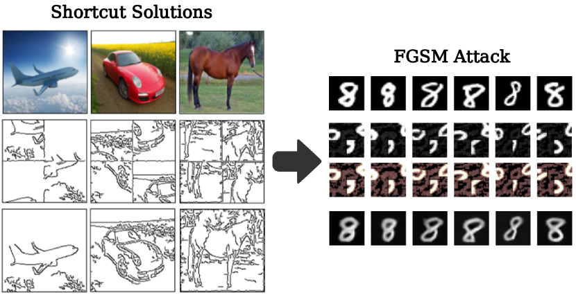
Figure 3: Some trivial features are produced that conduct the model to learn shortcuts. For example, model could understand the number of displacements just by noticing the vertical and horizontal lines. FGSM [38] makes specific anti-shortcut noises that appear similar to the number 8 (right figure). Heat map on the third row shows the normal image with better noise clarification.

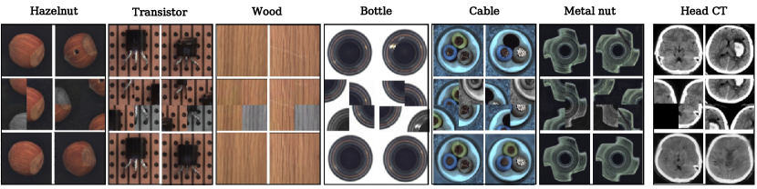
Figure 4: Visualization of the proposed method on MVTecAD [18] and Head CT datasets. First row is the original image, second row is the puzzled input mingled by colorization or inpainting and third row is the model’s output. For each category, first column is a normal input and the second column is an anomalous one.

Adversarial Training and Total Loss: The whole framework is also trained similar to the GAN framework [34] to improve the quality of the produced images. Better quality is obtained because of the ability of the adversarial training to converge to one mode despite MSE that converges to the average of different modes [39, 2, 40]. We define the reconstruction loss $\mathcal{L}_{rec}$ as the $\mathcal{L}_{2}$ distance between the original input $x$ which is drawn from the input data distribution $p_{x}$, and the solved puzzle at the output of the U-Net network $U(\tilde{f}_{P_{i}}(\tilde{x}))$:

$$\mathcal{L}_{rec}=\mathbb{E}_{x\sim p_{x}}\left\|U\left(\tilde{f}_{P_{i}}(\tilde{x})\right)-x\right\|_{2}.$$ (2)

Similar to [32], feature matching loss in the adversarial training is used. $f_{D}(\cdot)$ denotes a function representing an intermediate layer of our discriminator $D$. The adversarial loss $\mathcal{L}_{adv}$ is defined as follows:

$$\mathcal{L}_{adv}=\mathbb{E}_{x\sim p_{x}}\left\|f_{D}(x)-\mathbb{E}_{x\sim P_{x}}f_{D}\left(U\left(\tilde{f}_{P_{i}}(\tilde{x})\right)\right)\right\|_{2}.$$ (3)

Finally, the total loss used as our total training objective is defined as:

$$\mathcal{L}_{total}=\mathcal{L}_{rec}+\lambda\mathcal{L}_{adv},$$ (4)

where $\lambda$ is a hyper-parameter defining the weight of the $L_{adv}$ term in the total loss.

3.2 Anomaly Score

The same puzzle-making procedure is used for evaluation. We split each test data into 4 partitions and consider all the $K$ permutations of these partitions with at least 2 displacements without any inpainting or colorization auxiliary task. Suppose $x$ is a given test data and the $i^{\text{th}}$ permutation is used for the puzzle-making process to obtain $f_{P_{i}}(x)$. The anomaly score for this specific permutation is defined as:

$$\mathcal{S}^{\>i}_{test}=\|U(f_{P_{i}}(x))-x\|_{2}.$$ (5)

Error Normalization: Since solving each of the $K$ puzzles induce different difficulties for the model, the reconstruction error for some puzzles can be much larger than the others. Hence, different reconstruction errors can be obtained for a single input depending on the permutation used for the puzzle-making process. Therefore, we use validation data to normalize these errors over all the permutations. For this purpose, the average reconstruction error over all the validation data is computed for every single permutation. During test time, each reconstruction error is divided by the average error of validation data corresponding to that permutation :

$$\mathcal{S}_{test}^{\>\prime\;i}(x)=\frac{\|U(f_{P_{i}}(x))-x\|_{2}}{\mathbb{E}_{x\sim p_{x}}\|U(f_{P_{i}}(x))-x\|_{2}}.$$ (6)

Finally, min, max and average anomaly score for all the $K$ permutations of a single test data is computed:

$$\mathcal{S}_{test}(x)=\{\min\;\text{OR}\;\max\;\text{OR}\;avg\}_{1\leq i\leq K}\left\{\mathcal{S}_{test}^{\>\prime\;i}(x)\right\}.$$ (7)

The experiments show that using the max anomaly score is better for simple datasets, and as the dataset becomes more complex, using the average or min would yield better results. Therefore, to avoid unnecessary confusion and complexity in our performance measurement, we report the results by taking the max for the toy datasets and taking the average for the real-world datasets.

Fig. 4 shows the output of the model for some normal and anomalous inputs from MVTecAD [18] and Head CT (hemorrhage) dataset.

TABLE I: AUROC in % for several datasets. As it is shown, Puzzle-AE surpass the SOTA by 7% on average on the CIFAR-10 [12] dataset while it is still competitive on the other ones.

Dataset	Method	0	1	2	3	4	5	6	7	8	9	Mean
MNIST [41]	ARAE [37]	99.8	99.9	96.0	97.2	97.0	97.4	99.5	96.9	92.4	98.5	97.5
	OCSVM [42]	99.5	99.9	92.6	93.6	96.7	95.5	98.7	96.6	90.3	96.2	96.0
	AnoGAN [31]	96.6	99.2	85.0	88.7	89.4	88.3	94.7	93.5	84.9	92.4	91.3
	DSVDD [10]	98.0	99.7	91.7	91.9	94.9	88.5	98.3	94.6	93.9	96.5	94.8
	CapsNetPP [43]	99.8	99.0	98.4	97.6	93.5	97.0	94.2	98.7	99.3	99.0	97.7
	OCGAN [30]	99.8	99.9	94.2	96.3	97.5	98.0	99.1	98.1	93.9	98.1	97.5
	LSA [29]	99.3	99.9	95.9	96.6	95.6	96.4	99.4	98.0	95.3	98.1	97.5
	OURS	${99.6\pm 0.004}$	${99.93\pm 0.004}$	${97.12\pm 0.083}$	${96.97\pm 0.039}$	${97.70\pm 0.017}$	${98.43\pm 0.022}$	${99.29\pm 0.041}$	${98.26\pm 0.036}$	${94.14\pm 0.073}$	${98.57\pm 0.082}$	98.00
Fashion-MNIST [44]	ARAE [37]	93.7	99.1	91.1	94.4	92.3	91.4	83.6	98.9	93.9	97.9	93.6
	OCSVM [42]	91.9	99.0	89.4	94.2	90.7	91.8	83.4	98.8	90.3	98.2	92.8
	DAGMM [45]	30.3	31.1	47.5	48.1	49.9	41.3	42.0	37.4	51.8	37.8	41.7
	DSEBM [46]	89.1	56.0	86.1	90.3	88.4	85.9	78.2	98.1	86.5	96.7	85.5
	DSVDD [10]	98.2	90.3	90.7	94.2	89.4	91.8	83.4	98.8	91.9	99.0	92.8
	LSA [29]	91.6	98.3	87.8	92.3	89.7	90.7	84.1	97.7	91.0	98.4	92.2
	OURS(4-parts)	${91.37\pm 0.200}$	${98.96\pm 0.019}$	${89.34\pm 0.056}$	${92.04\pm 0.317}$	${91.04\pm 0.087}$	${90.73\pm 0.189}$	${82.39\pm 0.077}$	${98.23\pm 0.026}$	${91.02\pm 0.190}$	${97.52\pm 0.200}$	92.26
	OURS(9-parts)	${91.73\pm 0.621}$	${98.74\pm 0.133}$	${89.92\pm 0.252}$	${91.94\pm 0.612}$	${89.69\pm 0.566}$	${93.54\pm 0.606}$	${84.90\pm 0.405}$	${98.78\pm 0.078}$	${92.30\pm 1.178}$	${98.46\pm 0.169}$	93.00
CIFAR-10 [12]	ARAE [37]	72.2	43.1	69.0	55.0	75.2	54.7	70.1	51.0	72.2	40.0	60.23
	OCSVM [42]	63.0	44.0	64.9	48.7	73.5	50.0	72.5	53.3	64.9	50.8	58.56
	AnoGAN [31]	67.1	54.7	52.9	54.5	65.1	60.3	58.5	62.5	75.8	66.5	61.79
	DSVDD [10]	61.7	65.9	50.8	59.1	60.9	65.7	67.7	67.3	75.9	73.1	64.81
	CapsNetPP [43]	62.2	45.5	67.1	67.5	68.3	63.5	72.7	67.3	71.0	46.6	61.2
	OCGAN [30]	75.7	53.1	64.0	62.0	72.3	62.0	72.3	57.5	82.0	55.4	65.66
	LSA [29]	73.5	58.0	69.0	54.2	76.1	54.6	75.1	53.5	71.7	54.8	64.1
	OURS	${78.93\pm 0.203}$	${78.05\pm 0.755}$	${69.95\pm 0.344}$	${54.88\pm 0.410}$	${75.46\pm 0.204}$	${66.04\pm 0.430}$	${74.76\pm 0.280}$	${73.30\pm 0.468}$	${83.34\pm 0.256}$	${69.96\pm 0.461}$	72.47

4 Experiments

In this section, we validate our method by conducting extensive experiments. We consider multiple commonly used toy and also real-world datasets for evaluating our model.

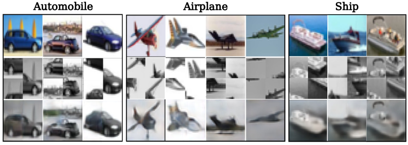
Figure 5: Effect of converting images to grayscale on the model learned features for some classes of CIFAR-10 [12] dataset. As it is shown, the model can produce perfect outputs even for grayscale inputs.

TABLE II: AUROC in % on MVTec AD [18] dataset. We surpass the SOTA by $\sim 4.6\%$.

Method	Bottle	Hazelnut	Capsule	Metal Nut	Leather	Pill	Wood	Carpet	Tile	Grid	Cable	Transistor	Toothbrush	Screw	Zipper	Mean
AVID [39]	88.0	86.0	85.0	63.0	58.0	86.0	83.0	70.0	66.0	59.0	64.0	58.0	73.0	66.0	84.0	73.0
AESSIM [47]	88.0	54.0	61.0	54.0	46.0	60.0	83.0	67.0	52.0	69.0	61.0	52.0	74.0	51.0	80.0	63.0
AEL2 [47]	80.0	88.0	62.0	73.0	44.0	62.0	74.0	50.0	77.0	78.0	56.0	71.0	98.0	69.0	80.0	71.0
AnoGAN [31]	69.0	50.0	58.0	50.0	52.0	62.0	68.0	49.0	51.0	51.0	53.0	67.0	57.0	35.0	59.0	55.0
LSA [29]	86.0	80.0	71.0	67.0	70.0	85.0	75.0	74.0	70.0	54.0	61.0	50.0	89.0	75.0	88.0	73.0
OURS	${94.24\pm 0.10}$	${91.21\pm 0.13}$	${66.88\pm 0.23}$	${66.33\pm 0.10}$	${72.86\pm 0.86}$	${71.63\pm 0.11}$	${89.51\pm 0.63}$	${65.73\pm 0.37}$	${65.48\pm 0.12}$	${75.35\pm 0.60}$	${87.90\pm 0.10}$	${85.96\pm 0.12}$	${97.79\pm 0.05}$	${57.81\pm 1.12}$	${75.74\pm 0.13}$	77.63

4.1 Experimental Setup

Datasets. We considered seven datasets for evaluating our method: MNIST, Fashion-MNIST, CIFAR-10, COIL-100, MVTecAD, and two medical datasets (Head CT (hemorrhage) and Brain MRI Images for Brain Tumor Detection). We briefly describe each of these datasets:
MNIST [41]: 60k training and 10k test $28\times 28$ gray-scale handwritten digit images from 0 to 9. Fashion-MNIST [44]: 60k training and 10k test grayscale images of 10 fashion product categories. CIFAR-10 [12]: 50k training and 10k test $32\times 32$ color images in 10 classes. COIL-100 [48]: 7200 $128\times 128$ color images of 100 object classes with 72 images of each object in different poses. MVTecAD [18]: an industrial dataset with more than 5k high-resolution images in 15 categories of objects and textures. Each category contains both normal and anomalous images with various kinds of defects (used for testing). We downscale all images to the size $128\times 128$ and use zoom data augmentation to create 800 training images for each class. Head CT (hemorrhage) [19]: a medical dataset containing 100 $128\times 128$ normal head CT images and 100 with hemorrhage. Brain MRI Images for Brain Tumor Detection [20]: a medical dataset with 98 $256\times 256$ normal MRI images and 155 with brain tumors.

Model Configuration and Hyperparameters. We used the standard U-Net architecture without the batchnorm layers [49] as our base framework, which is trained to reconstruct right order images. Moreover, the common discriminator introduced in DCGAN [50] was used as our next subnetwork, which was trained to classify the original input and output of the U-Net [35] as real or fake. We used the Adam optimizer [51] for training both networks. The learning rate was initially set to 1e-3 for the U-Net [35] and 2e-4 for the discriminator. We used a learning rate scheduler to multiply the learning rate by 0.8 when the minimum amount of loss did not change for 50 subsequent epochs [52]. Finally, we used the FGSM attack for robust adversarial training of the model. We trained the model until convergence of the loss function with a batch size of 8 for MVTecAD [18] and medical datasets and a batch size of 128 for the rest of the datasets.

Evaluating Protocols. The data partitioning used for the training-testing procedures is done similarly to [30] that introduces two protocols. We use Protocol 1 for the COIL-100 [53] dataset that randomly takes one class as the normal data and other classes as an anomaly. It uses 80% of all normal samples for the training and the rest for the test time normal samples. Test time anomalies are sampled from other classes until normal data, and anomalous ones are the same. This process is repeated 30 times, and the results are averaged. We randomly selected ten normal images for the medical datasets and used them along with the anomalous ones for the test data. The rest of the normal images were used for the training. For the MVTecAD [18] dataset, we use the given train and test sets for each class. Zoom augmentation is also performed to create 800 training images for each category of MVTecAD. Protocol 2 is used for all other datasets, which uses the whole training set of just one class as the normal data for training and the whole test set for the test time. We consider 15% of the training data as validation in each dataset. We evaluated the performance using the AUC of the ROC curve, which is commonly used for measuring performance in anomaly detection tasks.

4.2 Training and Testing Computational Cost

Because our method uses adversarial samples in its training process, one extra cost is added to our normal training process. To keep the additional cost to a minimum level, an FGSM attack has been used, which adds only one backpropagation to the training process. For the testing time, we compare our method with one of the best performing SOTA. To compare the execution time of our method with GT [17], we ran the CIFAR-10 experiment on the NVIDIA-GTX1080ti processor with 11 Gigabytes of RAM and with the same batch size. It has been observed that our testing routine has $4.7\times$ better execution performance than the GT algorithm, and it can become even faster by employing parallelism for finding each of the permutations’ costs. This faster execution time is beneficial in time-dependant anomaly detection tasks [1].

TABLE III: AUROC in % on COIL-100 [53] dataset. Obviously, Puzzle-AE reaches one of the SOTAs.

	COIL-100
Outlier Pursuit [54]	90.8
DPCP [55]	90.0
ALOCC DR [28]	80.9
ALOCC D [28]	68.6
GPND [56]	96.8
OCGAN [30]	99.5
OURS	99.3

TABLE IV: AUROC in % on real-world medical datasets. We have significant improvement with respect to the other AE-based SOTA methods.

		LSA* [29]	OCGAN* [30]	OURS
Head CT	AUC	${81.67\pm 0.358}$	${51.22\pm 3.626}$	${\textbf{86.43}\pm\textbf{0.04}}$
	FPR	0.81	1.00	0.70
Brain MRI	AUC	${95.61\pm 1.433}$	${91.74\pm 3.050}$	${\textbf{96.34}\pm\textbf{0.031}}$
	FPR	0.40	0.60	0.50

TABLE V: Significant better generalization of Puzzle-AE in compression with GT [17].

	GT [17]	OURS
MNIST [41]	98.00	98.00
CIFAR-10 [12]	82.30	72.47
MVTec [18]	$67.06*$	77.63
Head CT	$44.70^{*}$	86.43
Brain MRI	$82.07^{*}$	96.34

4.3 Results

In this section, our method’s results are compared with SOTA on the mentioned datasets. We report the mean and variance of our model AUC in the last 20 epochs of training. Other methods’ results are obtained from the main paper or reproduced from their officially released code.

AUC comparison with SOTA methods: The AUC results are presented for MNIST [41], Fashion-MNIST [44] and CIFAR-10 [12] in Table. I, in which Puzzle-AE is compared with the recent SOTAs on these datasets. Table. II shows comparison between Puzzle-AE and other SOTA methods on real-world, industrial dataset MVTecAD [18]. Table. III shows the results of Puzzle-AE on COIL-100 [53] dataset. To show the effectiveness and generalization properties of the proposed framework, two different experiments are conducted on two different medical datasets, and the results are presented in Table. IV. The results verify that Puzzle-AE performs significantly better than the competing methods. We also compared our method with a recent self-supervised learning method called GT [17], and the results are shown in Table. V. Moreover, while GT needs extra expert knowledge to design extra-large (72) unambiguous geometric transformations, Puzzle-AE is robust and does not need expert knowledge. Fig. 10 shows the brittleness of such transformations that become ambiguous with a low amount of noise for competing methods and also shows the robustness of Puzzle-AE in comparison to these methods.

AUC comparison with none-AE/AE based SSL methods on MVTecAD: Although GT [17] is an SSL based anomaly detector, we compare our method with other similar tasks to provide a more comprehensive comparison. In this part, the performance of our method is compared with the two of the most well-known SSL methods, such as jigsaw puzzle [24], and RotNet [57]. As it is shown in the Table. VI, similar to GT, these none AE-based SSL methods substantially fail on the real-world dataset MVTecAD. That is probably because they discard a lot of pixel-level information and only preserve as much as enough to solve their classification tasks. This is desirable, especially when dealing with semantic anomalies such as the CIFAR-10 dataset; however, as the results show, they are weak when dealing with subtle anomalies used in most industrial settings. We also compare puzzle-solving performance with the rotation prediction task implemented on our framework in ablation studies.

TABLE VI: The top rows shows AUROC in % for some of the fundamental none AE-based SSL methods on MVTecAD. The bottom row shows the AUROC in % of the Rot-AE on the similar dataset.

	Method	Bottle	Hazelnut	Capsule	Metal Nut	Leather	Pill	Wood	Carpet	Tile	Grid	Cable	Transistor	Toothbrush	Screw	Zipper	Mean
None AE-based SSL methods	Jigsaw puzzle [24]	38.41	57.96	41.28	52.74	12.6	47.71	46.49	35.79	24.13	60.48	33.62	24.00	35.56	51.24	8.95	37.93
	RotNet [57]	43.1	68.61	67.55	67.57	37.19	66.58	64.3	41.09	49.57	72.14	74.79	78.67	81.94	34.06	81	61.87
AE-based SSL method	Rot-AE	90.96	84.98	68.21	77.98	68.98	82.79	96.54	37.13	55.87	77.34	84.85	84.19	97.65	53.92	86.01	76.49

FPR comparison for high TPR: As discussed earlier, the two critical operating points of ROC curve are when TPR is equal to 99.0% or 99.5%. Table X shows that Puzzle-AE has significantly lower FPR in those critical points in comparison with LSA [29], while their difference in AUC is not significant.

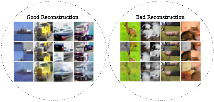
Figure 6: Anomalous reconstruction of the model trained on the class car of the CIFAR-10 [12] dataset. Good reconstruction occurs in classes with high similarity in main features such as truck and ship.

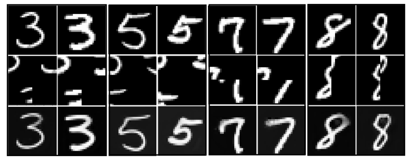
Figure 7: Visualization of the proposed method on MNIST [41] dataset. First row is the original input, second row is the puzzled input mingled by inpainting task and the third row is the unpuzzled output.

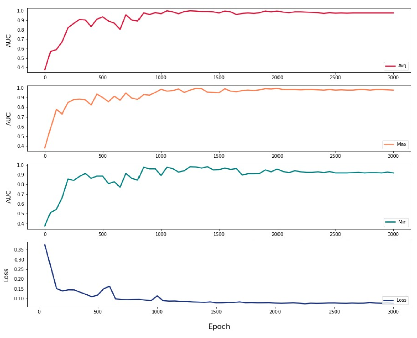
Figure 13: Min, max and avg AUC Plots with respect to training epochs are shown for the class toothbrush of the MVTecAD [18] dataset. As it is shown, training procedure continues till the convergence of all of the AUC plots and also loss value.

Model stability: Puzzle-AE has more stability in comparison with other methods. Fig. 13, 14, 15, 9, and tables I, II, IV show that we could achieve a highly reliable and stable model with the low variances at the end of the training phase. Moreover, because of using weight decay, the weights of our model are bounded, which is the consequence of Lipschitz continuity of Puzzle-AE.

Let $w$ denotes the weights of our model and let $\mathcal{L}$ be the total loss. Because of using weight decay, the main objective of the training procedure is defined as:

$$\min_{w}\;\;\mathcal{L}+c\|w\|_{\mathcal{F}}^{2}$$ (8)

where $\|\cdot\|_{\mathcal{F}}$ denotes the Frobenius norm and $c$ is a constant. This is equivalent to:

$$\min_{w}\;\mathcal{L}\;\;s.t.\;\;\|w\|_{\mathcal{F}}^{2}\leq M$$ (9)

which means that the model weights are bounded by some constant $M$. Also because all of the activation functions are smooth so have limited derivative value. This results in having limited upper bound for the whole network. Furthermore, Puzzle-AE produces smooth output, and it is shown that [58], being Lipschitz and smooth, the convergence of ADAM optimizer [51] is theoretically provable. This means that we could achieve a highly reliable and stable model at the end of the training phase. This is not the case for other methods such as GT [17] and DSVDD [10] as shown in the table VII where there are large fluctuations of AUC in different epochs of their training process. Because of using unprincipled early stopping methods that usually do not generalize well on unseen datasets, GT [17] AUC fluctuates nearly by 6% on the medical dataset and nearly 30% on MVTecAD [18] dataset while its training accuracy is above 98%.

Effect of training sample size on performance: Data efficiency, as another important feature that is desired in real-world applications, is shown in Fig. 8. Traditional AE based approaches usually need a rich dataset to model every complexity in data and obtain good generalization. However, As Fig. 8 illustrates, Puzzle-AE is significantly better than LSA [29] and DAE [59] in terms of data efficiency that is because of its different mean to model abstractions. It is also shown in table IX that not only Puzzle-AE is significantly better than other SOTA AE-based approaches but also is better than DSVDD [10] which is a one-class method.

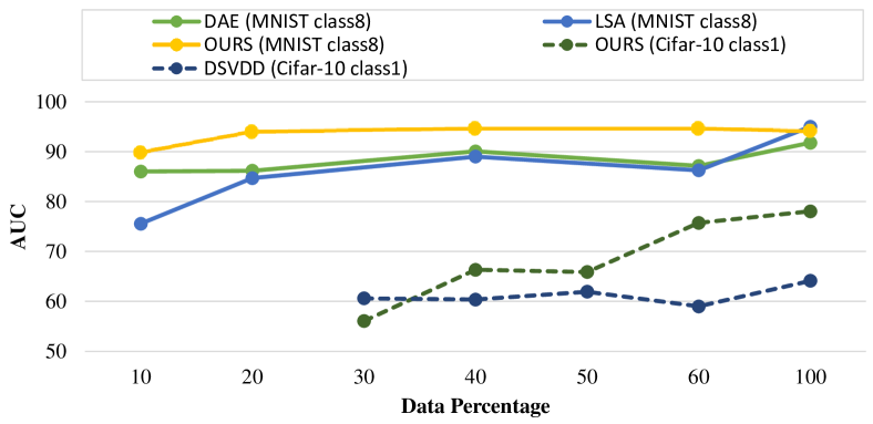
Figure 8: Puzzle-AE is significantly more data efficient than LSA [29] and DAE [59] on the class 8 of the MNIST [41] dataset. Puzzle-AE also performs better than DSVDD [10] in the class car of the CIFAR-10 [12] dataset.

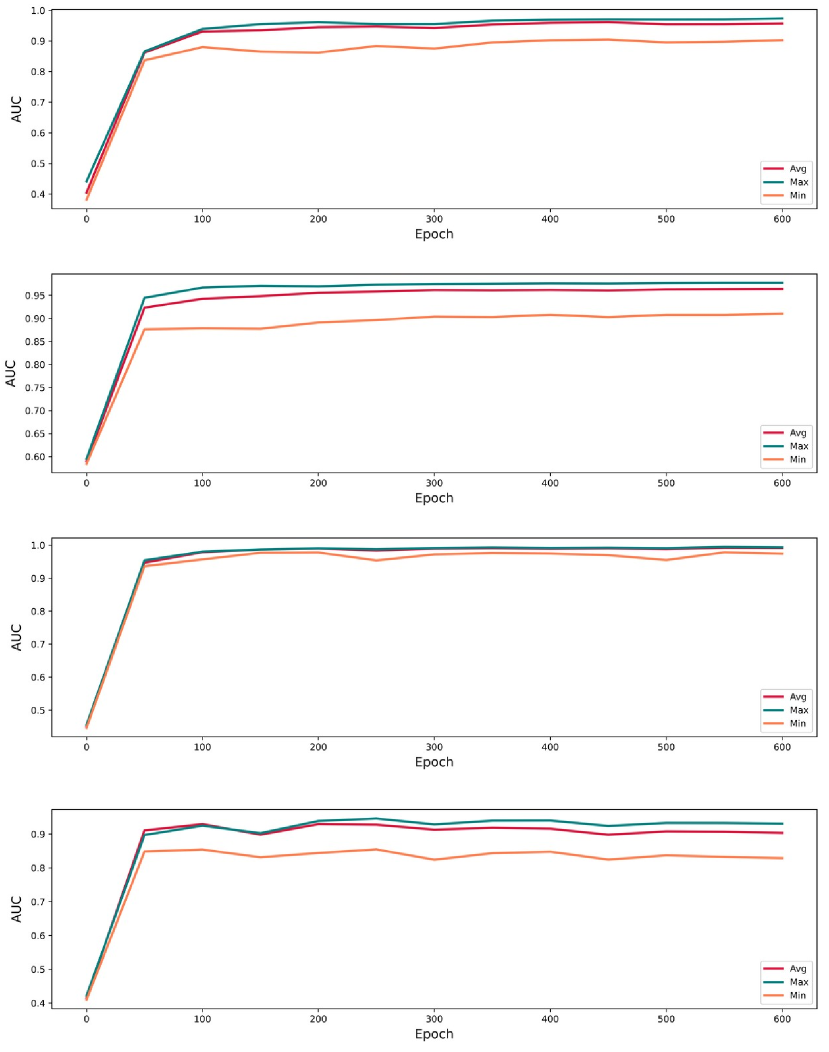
Figure 9: Min, max and avg AUC Plots with respect to training epochs are shown for the classes 2, 4, 6 and 8 of the MNIST [41] dataset.

Robustness through attacked normal samples: Robustness against attacked normal images was examined and the results are reported in Fig. 10. As it is shown, Puzzle-AE is significantly more robust against attacks to normal images with three different values of $\epsilon$ ($0.05,0.1$ and $0.2$) in comparison with LSA [29], ARAE [37] and GT [17]. To explain different attacks applied to our method in attack1, we apply FGSM [38] attack on the normal class before permutation. However, in attack2, we apply FGSM [38] attack on the permuted image. The attacked image is brought back to the original form by using the corresponding inverse permutation. By averaging over all possible permutations, the attacked version of the normal class is obtained.

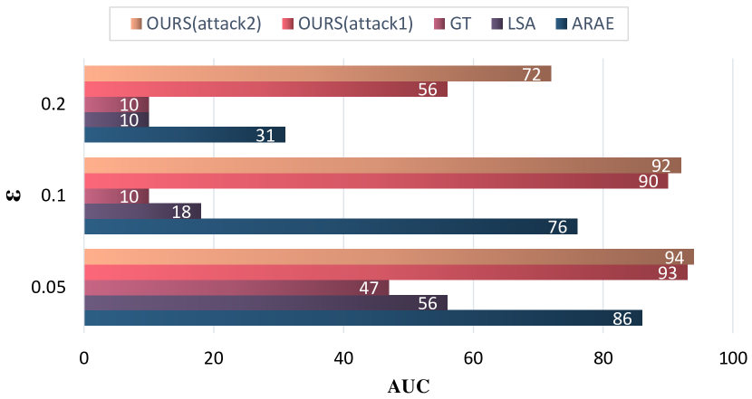
Figure 10: Robustness to adversarial attack on normal data at testing time. The results are shown for three different $\epsilon$ and the model is trained on class 8 of the MNIST [41] dataset.

Visualization of Puzzle-AE on Different Datasets: Sample images from different datasets are shown in Fig. 11, 7, and 12. In each image, the first row shows the original input; the second row is the puzzled input mingled by one of the inpainting or colorization tasks. The final unpuzzled output of the model is shown in the third row.

Figure 11: Visualization of the proposed method on CIFAR-10 [12] dataset. First row is the original input, second row is the puzzled input mingled by colorization task and the third row is the unpuzzled output.

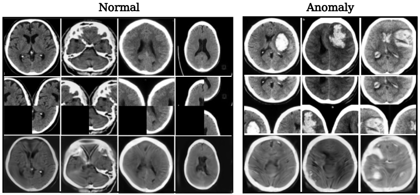
Figure 12: Visualization of the proposed method on Head CT dataset. First row is the original input, second row is the puzzled input mingled by the inpainting task, and the third row is the unpuzzled output solved by the model.

Fig. 6 shows outputs of the model trained on the class car of the CIFAR-10 [12] dataset for some anomalous inputs.

TABLE VII: Up - GT [17] AUC fluctuations during training procedure on head ct medical and the capsule class of MVTecAD [18] dataset. Bottom - DSVDD [10] AUC fluctuations during last 16 epochs of training procedure on the class car of CIFAR-10 [12] dataset.

Method	Dataset		0	1	2	3	4	5	6	7	8	9	10	11	12	13	14	15	16
GT [17]	Head CT	AUC	56.52	53.68	54.26	69.29	67.10	69.87	77.48	79.03	76.45	77.48	79.55	80.06	81.23	80.90	77.68	79.23	75.03
		Train ACC	14.59	34.45	43.41	55.84	71.17	90.08	98.88	99.92	99.98	100	100	100	100	100	99.93	99.60	98.14
	MVTec (Capsule)	AUC	45.95	67.41	71.20	74.11	77.46	60.75	64.10	73.00	73.00	62.82	62.50	66.29	69.49	60.63	66.85	73.35	68.93
		Train ACC	98.89	99.50	100	100	100	99.99	100	100	100	100	100	99.55	100	98.49	100	100	100
DSVDD [10]	Cifar-10 (Car)	AUC	56.21	51.83	53.74	54.50	57.57	59.86	60.23	60.60	59.81	56.37	57.72	55.82	58.40	54.04	54.97	55.25	56.22
		Train loss	0.577	0.477	0.387	0.332	0.328	0.314	0.306	0.300	0.288	0.282	0.267	0.259	0.251	0.242	0.229	0.218	0.211

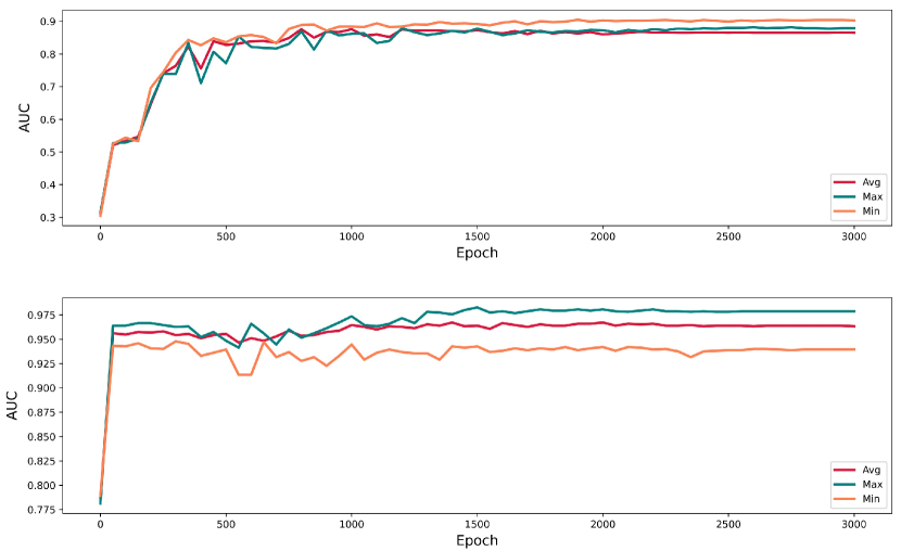
Figure 14: Min, max and avg AUC Plots with respect to training epochs are shown for each medical dataset.

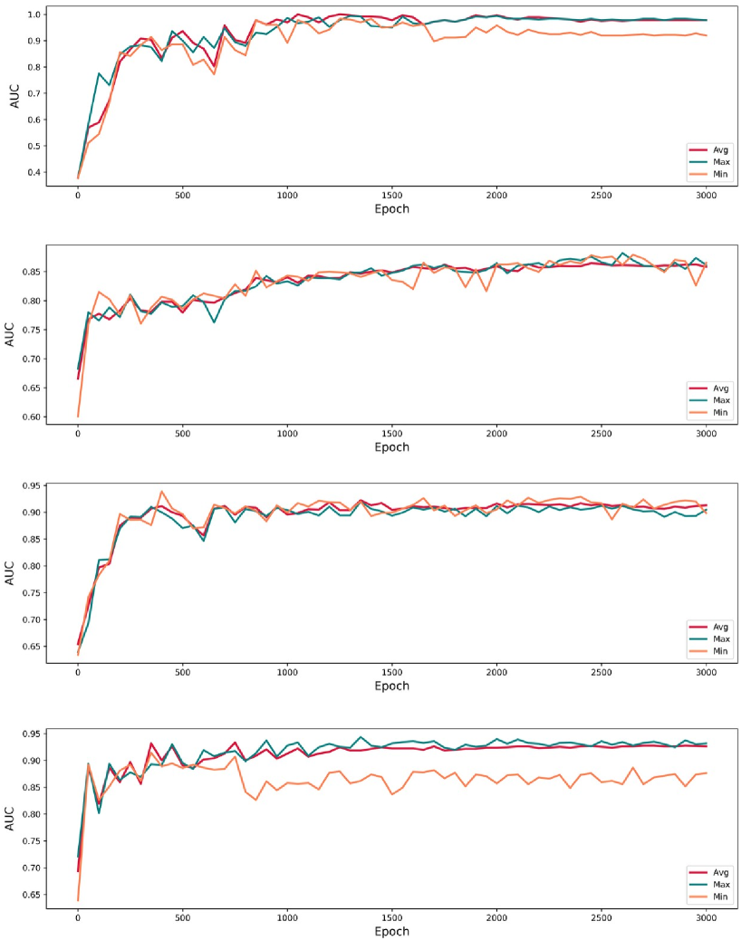
Figure 15: Min, max and avg AUC Plots with respect to training epochs are shown for the classes toothbrush, transistor, hazelnut and bottle of the MVTecAD [18] dataset.

5 Ablation

In this section, the effects of several important parameters are examined, as follows:

1. Effect of Each Component of the Puzzle-AE on Final Performance: Table. VIII shows the effect of every single module or algorithm that has been used in this framework on the CIFAR-10 [12] dataset. The results are shown for puzzle-solving AE (PAE), puzzle-solving and colorization (CPAE), and also CPAE combined with adversarial training (CPAE-G). The results show that each of these parts has an important role in gaining the best possible performance.

   TABLE VIII: Effect of each component or algorithm is illustrated separately. As it is shown, CPAE-G has the best results on sample dataset CIFAR-10 [12].

   		0	1	2	3	4	5	6	7	8	9	mean
   MIN	puzzle AE (PAE)	76.32	69.69	68.70	54.08	75.30	62.91	72.72	69.61	80.87	64.88	69.51
   	colorization + puzzle (CPAE)	79.51	69.77	68.51	54.75	72.56	63.24	67.86	68.30	82.09	65.57	69.22
   	colorization + puzzle + GAN (CPAE-G)	79.42	73.00	69.48	53.00	73.98	65.13	68.98	70.65	83.28	66.73	70.37
   MAX	puzzle AE (PAE)	76.29	69.07	68.19	52.14	75.84	60.84	73.66	68.61	78.26	66.20	68.91
   	colorization + puzzle (CPAE)	78.87	76.56	67.97	54.33	74.69	62.32	75.72	71.59	81.06	70.92	71.40
   	colorization + puzzle + GAN (CPAE-G)	77.21	77.31	69.3	54.10	74.76	64.10	76.02	70.42	81.04	66.91	71.12
   AVG	puzzle AE (PAE)	76.59	68.84	68.54	53.00	76.00	61.8	73.32	68.87	79.54	66.12	69.26
   	colorization + puzzle (CPAE)	79.72	75.86	68.56	54.74	74.87	64.21	74.02	72.97	82.64	70.62	71.82
   	colorization + puzzle + GAN (CPAE-G)	78.93	78.05	69.95	54.88	75.46	66.04	74.76	73.30	83.34	69.96	72.47

2. Effect of Puzzle Solving Compare to Rotation as the SSL Task: As the Table. VI reports, the performance of the rotation task is 1% lesser than our method on the average of 15 classes. That is because of the rotation invariant aspect existing in most of the texture classes. As mentioned earlier, the puzzle-solving task is less ambiguous for different datasets than rotation prediction, which means we have lesser presumptions on training datasets for various problems.

3. Effect of converting pictures to gray-scale on performance: It was observed that extracted normal features of Puzzle-AE are less sensitive to color for some specific classes of the CIFAR-10 [12] dataset. For example, no significant performance drop was observed on the class car of CIFAR-10 [12] when converting the whole dataset to gray-scale. Fig. 5 shows the ability of the proposed model in solving unseen gray-scale puzzled inputs.

4. Effect of PGD [26], FGSM [38]: It was observed that PGD [26] and FGSM [38] have almost similar effects on the performance. They provide about 1% improvement on datasets that have obvious shortcuts, such as MNIST. However, their role would be more significant in the robustification of the framework.

TABLE IX: Puzzle-AE has  6% and  3% better performances when trained on the MNIST [41] with 1/12 samples with respect to LSA [29] and DSVDD [10].

Method	0	1	2	3	4	5	6	7	8	9	mean
LSA* [29]	${95.93\pm 0.087}$	${99.82\pm 0.005}$	${80.95\pm 0.119}$	${83.95\pm 0.090}$	${87.59\pm 0.113}$	${85.81\pm 0.072}$	${92.61\pm 0.059}$	${93.31\pm 0.074}$	${76.56\pm 0.328}$	${92.40\pm 0.075}$	88.89
DSVDD* [10]	${96.10\pm 0.057}$	${99.17\pm 0.006}$	${88.62\pm 0.146}$	${86.60\pm 0.252}$	${95.09\pm 0.024}$	${84.93\pm 0.091}$	${96.40\pm 0.058}$	${94.68\pm 0.036}$	${89.76\pm 0.121}$	${94.72\pm 0.044}$	92.61
OURS	${99.54\pm 0.044}$	${99.73\pm 0.034}$	${90.41\pm 0.593}$	${89.59\pm 1.056}$	${95.71\pm 0.306}$	${96.79\pm 0.504}$	${97.23\pm 0.310}$	${96.98\pm 0.189}$	${89.81\pm 0.676}$	${93.17\pm 0.592}$	94.90

TABLE X: Puzzle-AE has significantly better TPR at FPR equal to 99.5% and 99.0% than LSA [29] on the MNIST [41] dataset for 10 class average.

TPR	Method	0	1	2	3	4	5	6	7	8	9	Mean
99%	LSA* [29]	0.0765	0.0088	0.7238	0.4119	0.6365	0.3274	0.1190	0.4591	0.5975	0.2428	0.3603
	OURS	0.0480	0.0053	0.3295	0.2079	0.3157	0.1939	0.1086	0.2451	0.7156	0.1724	0.2342
99.5%	LSA* [29]	0.0980	0.0123	0.8178	0.4871	0.7210	0.3924	0.1587	0.5447	0.7146	0.3142	0.4261
	OURS	0.0694	0.0088	0.4079	0.2545	0.4287	0.3262	0.1441	0.2977	0.7895	0.2061	0.2932

6 Conclusion and Future Work

In this study, we have tackled two significant problems of AEs. Using a U-Net that solves puzzled inputs, the quality of reconstructed normal test time inputs is increased, and the inability to reconstruct anomalous samples is kept. The experimental results show significant improvements in stability, robustness, data efficiency, generality, and FPR at high TPRs on a wide gamut of datasets. For the future works, some solutions for the several deficiencies of our method, such as solving some anomalous puzzled inputs, as is shown in the Fig. 6 will be investigated. Moreover, a quantitative criterion for selecting min, max, or the average of the anomaly score could improve the results for future works.

Mohammadreza Salehi received his B.Sc. degree in computer engineering from the University of Tehran in 2018. He is currently an M.Sc. student in the Department of Computer Engineering, Sharif University of Technology. His research interests include computer vision and machine learning, focusing on anomaly detection in image and video.

Ainaz Eftekhar is currently pursuing her B.Sc. degree in the Department of Computer Engineering at the Sharif University of Technology. She is working as a researcher in the Robust and Interpretable ML Lab and as a remote research assistant in Visual Intelligence and Learning Laboratory (VILAB) at EPFL. Her research interests include computer vision, machine learning, and AI.

Niousha Sadjadi is a senior undergraduate student in the Department of Computer Engineering at the Sharif University of Technology. Currently, she works as a researcher on different anomaly detection methods in the Robust and Interpretable ML lab. Her research interests include computer vision, unsupervised learning, neural computing, and anomaly detection on images.

Mohammad Hossein Rohban received his BS, MS ad Ph.D. degrees in Computer Engineering from the Sharif University of Technology. Currently, he is an assistant professor in the Department of Computer Engineering at the Sharif University of Technology. His current research interests include interpretable and robust machine learning, anomaly detection, and computational Biology. He previously spent three years as a postdoctoral associate at the Broad Institute of Harvard and MIT. He focused on various problems at the intersection of machine learning and image-based Computational Biology, where he published several prestigious papers on the mentioned subjects in the relevant journals.

Hamid R. Rabiee (SM ’07) received his BS and MS degrees (with Great Distinction) in Electrical Engineering from CSULB, Long Beach, CA (1987, 1989), his EEE degree in Electrical and Computer Engineering from USC, Los Angeles, CA (1993), and his Ph.D. in Electrical and Computer Engineering from Purdue University, West Lafayette, IN, in 1996. From 1993 to 1996, he was a Member of the Technical Staff at AT&T Bell Laboratories. From 1996 to 1999, he worked as a Senior Software Engineer at Intel Corporation. He was also with PSU, OGI, and OSU universities as an adjunct professor of Electrical and Computer Engineering from 1996-2000. Since September 2000, he has joined the Sharif University of Technology, Tehran, Iran. He was also a visiting professor at the Imperial College of London for the 2017-2018 academic year. He is the founder of Sharif University Advanced Information and Communication Technology Research Institute (AICT), ICT Innovation Center, Advanced Technologies Incubator (SATI), Digital Media Laboratory (DML), Mobile Value Added Services Laboratory (VASL), Bioinformatics and Computational Biology Laboratory (BCB) and Cognitive Neuroengineering Research Center. He is also a consultant and member of AI in Health Expert Group at WHO. He has been the founder of many successful High-Tech start-up companies in ICT as an entrepreneur. He is currently a Professor of Computer Engineering at Sharif University of Technology, and Director of AICT, DML, and VASL. He has received numerous awards and honors for his Industrial, scientific, and academic contributions and holds three patents. His research interests include statistical machine learning, Bayesian statistics, data analytics, and complex networks with applications in social networks, multimedia systems, cloud and IoT privacy, bioinformatics, and brain networks.

References

- [1] R. Chalapathy and S. Chawla, “Deep learning for anomaly detection: A survey,” arXiv preprint arXiv:1901.03407, 2019.
- [2] X. Chen and E. Konukoglu, “Unsupervised detection of lesions in brain mri using constrained adversarial auto-encoders,” arXiv preprint arXiv:1806.04972, 2018.
- [3] C. Baur, B. Wiestler, S. Albarqouni, and N. Navab, “Deep autoencoding models for unsupervised anomaly segmentation in brain mr images,” in International MICCAI Brainlesion Workshop. Springer, 2018, pp. 161–169.
- [4] D. Gong, L. Liu, V. Le, B. Saha, M. R. Mansour, S. Venkatesh, and A. v. d. Hengel, “Memorizing normality to detect anomaly: Memory-augmented deep autoencoder for unsupervised anomaly detection,” in Proceedings of the IEEE International Conference on Computer Vision, 2019, pp. 1705–1714.
- [5] I. Goodfellow, “Nips 2016 tutorial: Generative adversarial networks,” arXiv preprint arXiv:1701.00160, 2016.
- [6] N. Kodali, J. Abernethy, J. Hays, and Z. Kira, “On convergence and stability of gans,” arXiv preprint arXiv:1705.07215, 2017.
- [7] T. Salimans, I. Goodfellow, W. Zaremba, V. Cheung, A. Radford, and X. Chen, “Improved techniques for training gans,” in Advances in neural information processing systems, 2016, pp. 2234–2242.
- [8] A. Martin and B. Lon, “Towards principled methods for training generative adversarial networks,” in NIPS 2016 Workshop on Adversarial Training. In review for ICLR, vol. 2016, 2017.
- [9] E. Nalisnick, A. Matsukawa, Y. W. Teh, D. Gorur, and B. Lakshminarayanan, “Do deep generative models know what they don’t know?” arXiv preprint arXiv:1810.09136, 2018.
- [10] L. Ruff, R. Vandermeulen, N. Goernitz, L. Deecke, S. A. Siddiqui, A. Binder, E. Müller, and M. Kloft, “Deep one-class classification,” in International conference on machine learning, 2018, pp. 4393–4402.
- [11] M. Sakurada and T. Yairi, “Anomaly detection using autoencoders with nonlinear dimensionality reduction,” in Proceedings of the MLSDA 2014 2nd Workshop on Machine Learning for Sensory Data Analysis, 2014, pp. 4–11.
- [12] A. Krizhevsky, V. Nair, and G. Hinton, “Cifar-10 (canadian institute for advanced research),” 2009.
- [13] J. Deng, W. Dong, R. Socher, L.-J. Li, K. Li, and L. Fei-Fei, “Imagenet: A large-scale hierarchical image database,” in 2009 IEEE conference on computer vision and pattern recognition. Ieee, 2009, pp. 248–255.
- [14] Z. Wu, Y. Xiong, S. X. Yu, and D. Lin, “Unsupervised feature learning via non-parametric instance discrimination,” in Proceedings of the IEEE Conference on Computer Vision and Pattern Recognition, 2018, pp. 3733–3742.
- [15] A. v. d. Oord, Y. Li, and O. Vinyals, “Representation learning with contrastive predictive coding,” arXiv preprint arXiv:1807.03748, 2018.
- [16] R. Zhang, P. Isola, and A. A. Efros, “Split-brain autoencoders: Unsupervised learning by cross-channel prediction,” in Proceedings of the IEEE Conference on Computer Vision and Pattern Recognition, 2017, pp. 1058–1067.
- [17] I. Golan and R. El-Yaniv, “Deep anomaly detection using geometric transformations,” in Advances in Neural Information Processing Systems, 2018, pp. 9758–9769.
- [18] P. Bergmann, M. Fauser, D. Sattlegger, and C. Steger, “Mvtec ad–a comprehensive real-world dataset for unsupervised anomaly detection,” in Proceedings of the IEEE Conference on Computer Vision and Pattern Recognition, 2019, pp. 9592–9600.
- [19] F. Kitamura, “Head ct - hemorrhage,” https://www.kaggle.com/felipekitamura/head-ct-hemorrhage, 2018.
- [20] N. Chakrabarty, “Brain mri images for brain tumor detection,” https://www.kaggle.com/navoneel/brain-mri-images-for-brain-tumor-detection, 2019.
- [21] O. Ronneberger, P. Fischer, and T. Brox, “U-net: Convolutional networks for biomedical image segmentation,” in International Conference on Medical image computing and computer-assisted intervention. Springer, 2015, pp. 234–241.
- [22] V. Badrinarayanan, A. Kendall, and R. Cipolla, “Segnet: A deep convolutional encoder-decoder architecture for image segmentation,” IEEE transactions on pattern analysis and machine intelligence, vol. 39, no. 12, pp. 2481–2495, 2017.
- [23] G. Litjens, T. Kooi, B. E. Bejnordi, A. A. A. Setio, F. Ciompi, M. Ghafoorian, J. A. Van Der Laak, B. Van Ginneken, and C. I. Sánchez, “A survey on deep learning in medical image analysis,” Medical image analysis, vol. 42, pp. 60–88, 2017.
- [24] M. Noroozi and P. Favaro, “Unsupervised learning of visual representations by solving jigsaw puzzles,” in European Conference on Computer Vision. Springer, 2016, pp. 69–84.
- [25] D. Hendrycks, M. Mazeika, S. Kadavath, and D. Song, “Using self-supervised learning can improve model robustness and uncertainty,” in Advances in Neural Information Processing Systems, 2019, pp. 15 663–15 674.
- [26] A. Madry, A. Makelov, L. Schmidt, D. Tsipras, and A. Vladu, “Towards deep learning models resistant to adversarial attacks,” arXiv preprint arXiv:1706.06083, 2017.
- [27] A. Ilyas, S. Santurkar, D. Tsipras, L. Engstrom, B. Tran, and A. Madry, “Adversarial examples are not bugs, they are features,” in Advances in Neural Information Processing Systems, 2019, pp. 125–136.
- [28] M. Sabokrou, M. Khalooei, M. Fathy, and E. Adeli, “Adversarially learned one-class classifier for novelty detection,” in Proceedings of the IEEE Conference on Computer Vision and Pattern Recognition, 2018, pp. 3379–3388.
- [29] D. Abati, A. Porrello, S. Calderara, and R. Cucchiara, “Latent space autoregression for novelty detection,” in Proceedings of the IEEE Conference on Computer Vision and Pattern Recognition, 2019, pp. 481–490.
- [30] P. Perera, R. Nallapati, and B. Xiang, “Ocgan: One-class novelty detection using gans with constrained latent representations,” in Proceedings of the IEEE Conference on Computer Vision and Pattern Recognition, 2019, pp. 2898–2906.
- [31] T. Schlegl, P. Seeböck, S. M. Waldstein, U. Schmidt-Erfurth, and G. Langs, “Unsupervised anomaly detection with generative adversarial networks to guide marker discovery,” in International conference on information processing in medical imaging. Springer, 2017, pp. 146–157.
- [32] S. Akcay, A. Atapour-Abarghouei, and T. P. Breckon, “Ganomaly: Semi-supervised anomaly detection via adversarial training,” in Asian Conference on Computer Vision. Springer, 2018, pp. 622–637.
- [33] D. P. Kingma and M. Welling, “Auto-encoding variational bayes,” arXiv preprint arXiv:1312.6114, 2013.
- [34] I. J. Goodfellow, J. Shlens, and C. Szegedy, “Explaining and harnessing adversarial examples,” arXiv preprint arXiv:1412.6572, 2014.
- [35] X. Li, H. Chen, X. Qi, Q. Dou, C.-W. Fu, and P.-A. Heng, “H-denseunet: hybrid densely connected unet for liver and tumor segmentation from ct volumes,” IEEE transactions on medical imaging, vol. 37, no. 12, pp. 2663–2674, 2018.
- [36] X. Wang, Y. Peng, L. Lu, Z. Lu, M. Bagheri, and R. M. Summers, “Chestx-ray8: Hospital-scale chest x-ray database and benchmarks on weakly-supervised classification and localization of common thorax diseases,” in Proceedings of the IEEE conference on computer vision and pattern recognition, 2017, pp. 2097–2106.
- [37] M. Salehi, A. Arya, B. Pajoum, M. Otoofi, A. Shaeiri, M. H. Rohban, and H. R. Rabiee, “Arae: Adversarially robust training of autoencoders improves novelty detection,” arXiv preprint arXiv:2003.05669, 2020.
- [38] E. Wong, L. Rice, and J. Z. Kolter, “Fast is better than free: Revisiting adversarial training,” arXiv preprint arXiv:2001.03994, 2020.
- [39] M. Sabokrou, M. Pourreza, M. Fayyaz, R. Entezari, M. Fathy, J. Gall, and E. Adeli, “Avid: Adversarial visual irregularity detection,” in Asian Conference on Computer Vision. Springer, 2018, pp. 488–505.
- [40] I. Tolstikhin, O. Bousquet, S. Gelly, and B. Schoelkopf, “Wasserstein auto-encoders,” arXiv preprint arXiv:1711.01558, 2017.
- [41] Y. LeCun, C. Cortes, and C. Burges, “Mnist handwritten digit database,” 2010.
- [42] Y. Chen, X. S. Zhou, and T. S. Huang, “One-class svm for learning in image retrieval,” in Proceedings 2001 International Conference on Image Processing (Cat. No. 01CH37205), vol. 1. IEEE, 2001, pp. 34–37.
- [43] X. Li, I. Kiringa, T. Yeap, X. Zhu, and Y. Li, “Exploring deep anomaly detection methods based on capsule net,” in ICML 2019 Workshop on Uncertainty and Robustness in Deep Learning, At Long Beach, 2019.
- [44] H. Xiao, K. Rasul, and R. Vollgraf, “Fashion-mnist: a novel image dataset for benchmarking machine learning algorithms,” arXiv preprint arXiv:1708.07747, 2017.
- [45] B. Zong, Q. Song, M. R. Min, W. Cheng, C. Lumezanu, D. Cho, and H. Chen, “Deep autoencoding gaussian mixture model for unsupervised anomaly detection,” 2018.
- [46] S. Zhai, Y. Cheng, W. Lu, and Z. Zhang, “Deep structured energy based models for anomaly detection,” arXiv preprint arXiv:1605.07717, 2016.
- [47] P. Bergmann, S. Löwe, M. Fauser, D. Sattlegger, and C. Steger, “Improving unsupervised defect segmentation by applying structural similarity to autoencoders,” in International Joint Conference on Computer Vision, Imaging and Computer Graphics Theory and Applications (VISIGRAPP), 2019.
- [48] S. A. Nene, S. K. Nayar, H. Murase et al., “Columbia object image library (coil-100),” 1996.
- [49] S. Ioffe and C. Szegedy, “Batch normalization: Accelerating deep network training by reducing internal covariate shift,” arXiv preprint arXiv:1502.03167, 2015.
- [50] A. Radford, L. Metz, and S. Chintala, “Unsupervised representation learning with deep convolutional generative adversarial networks,” arXiv preprint arXiv:1511.06434, 2015.
- [51] D. P. Kingma and J. Ba, “Adam: A method for stochastic optimization,” arXiv preprint arXiv:1412.6980, 2014.
- [52] P. Goyal, P. Dollár, R. Girshick, P. Noordhuis, L. Wesolowski, A. Kyrola, A. Tulloch, Y. Jia, and K. He, “Accurate, large minibatch sgd: Training imagenet in 1 hour,” arXiv preprint arXiv:1706.02677, 2017.
- [53] S. A. Nene, S. K. Nayar, and H. Murase, “object image library (coil-100,” Tech. Rep., 1996.
- [54] H. Xu, C. Caramanis, and S. Sanghavi, “Robust pca via outlier pursuit,” in Advances in Neural Information Processing Systems, 2010, pp. 2496–2504.
- [55] M. C. Tsakiris and R. Vidal, “Dual principal component pursuit,” The Journal of Machine Learning Research, vol. 19, no. 1, pp. 684–732, 2018.
- [56] S. Pidhorskyi, R. Almohsen, and G. Doretto, “Generative probabilistic novelty detection with adversarial autoencoders,” in Advances in neural information processing systems, 2018, pp. 6822–6833.
- [57] S. Gidaris, P. Singh, and N. Komodakis, “Unsupervised representation learning by predicting image rotations,” arXiv preprint arXiv:1803.07728, 2018.
- [58] X. Chen, S. Liu, R. Sun, and M. Hong, “On the convergence of a class of adam-type algorithms for non-convex optimization,” arXiv preprint arXiv:1808.02941, 2018.
- [59] P. Vincent, H. Larochelle, Y. Bengio, and P.-A. Manzagol, “Extracting and composing robust features with denoising autoencoders,” in Proceedings of the 25th international conference on Machine learning, 2008, pp. 1096–1103.