On the model-based stochastic value gradient for continuous reinforcement learning

Abstract

For over a decade, model-based reinforcement learning has been seen as a way to leverage control-based domain knowledge to improve the sample-efficiency of reinforcement learning agents. While model-based agents are conceptually appealing, their policies tend to lag behind those of model-free agents in terms of final reward, especially in non-trivial environments. In response, researchers have proposed model-based agents with increasingly complex components, from ensembles of probabilistic dynamics models, to heuristics for mitigating model error. In a reversal of this trend, we show that simple model-based agents can be derived from existing ideas that not only match, but outperform state-of-the-art model-free agents in terms of both sample-efficiency and final reward. We find that a model-free soft value estimate for policy evaluation and a model-based stochastic value gradient for policy improvement is an effective combination, achieving state-of-the-art results on a high-dimensional humanoid control task, which most model-based agents are unable to solve. Our findings suggest that model-based policy evaluation deserves closer attention.

Source Code: github.com/facebookresearch/svg

1 Introduction

The task of designing a reinforcement learning (RL) agent that can learn to optimally interact with an unknown environment has wide-reaching applications in, e.g., robotics [41, 59], control [48, 39], finance [20], and gaming [75, 5, 37]. Many long-standing challenges remain after decades of research [68] and the field is unsettled on a single method for solving classes of tasks. Subtle variations in the settings can significantly impact how agents need to learn, explore, and represent their internal decision process and the external world around them.

Model-based methods explicitly construct a surrogate of the true environment, which can be queried with hypothetical sequences of actions to assess their outcome. In contrast, model-free methods rely entirely on online and historical ground-truth data, and implicitly incorporate the environment dynamics into action value estimates. Historically, the abstractions of model-based methods are more amenable to the incorporation of expert domain knowledge [71], and often find higher reward policies than their model-free counterparts when only a small amount of ground-truth data can be collected [16, 12, 77, 35, 38]. However model-based methods struggle to match the performance of model-free agents when the latter are allowed unlimited interactions with the environment. While recent work has greatly improved the asymptotic performance of model-based agents, on the most challenging tasks they still often significantly under-perform model-free approaches.

While the incorporation of an explicit world model can introduce helpful inductive biases to RL agents, imperfect learned models introduce additional, unwanted biases. An imperfect model may assign high expected reward to catastrophic actions, or it may conjure fantasies of hypothetical states having no correspondence to any realizable agent configuration. Precisely which biases are introduced, and the resulting impact on the agent, depends heavily on how the model is used. In some cases, the model aids action selection online, and in others it augments an existing replay buffer with fictional experience. The reproducibility crisis in reinforcement learning [34, 32, 18, 65] makes evaluating and understanding the tradeoffs difficult.

In this work we seek to answer a key question: “What is the simplest model-based agent that can achieve state-of-the-art results on current benchmark tasks?” We show that if the model is used only for policy improvement, then a simple combination of a stochastic value gradient (SVG) [31], entropy regularization, soft value estimates [27], and a single deterministic dynamics model are sufficient to match and surpass the performance of model-based and model-free methods. This finding is particularly notable because our baselines are substantially stronger than those reported in previous work. We also show that the performance improvements of our approach cannot be attributed to model architecture alone. Finally, we demonstrate that policy evaluation can be significantly more sensitive to model bias than policy improvement, even for short rollouts.

Figure 1: A model-based SAC-SVG agent learns a near-optimal humanoid gait by using short-horizon model rollouts. More videos are online at sites.google.com/view/2020-svg.

2 Related work on model-based continuous reinforcement learning

In most model-based methods for continuous control, the dynamics model serves some or all of the following functions: (1) a source of low-bias on-policy value estimates, obtained by explicitly unrolling the policy for the full horizon or by refining a bootstrapped value estimate; (2) a source of multistep value gradients for policy improvement; or (3) a source of fictional transition data with which to augment expensive ground-truth transition data for standard model-free updates. Nearly every combination of these three functions can be found in the literature. If bootstrapped value estimates are not used, and the model fulfills functions (1) and (2), one obtains a generalized form of PILCO [16]. Introducing bootstrapped value estimates and removing (1), one obtains the value gradient [31, 9, 28, 13]. The model with (1) can also be used in a search procedure [66, 49]. Conversely if (1) is retained and (2) is removed, the MVE method [19] is recovered. Dyna-Q [67] is an early method which uses the model exclusively for (3), followed more recently by NAF [25], ME-TRPO [44], and MBPO [35]. Other contributions focus on the effect of ensembling some or all of the learned models, such as PETS [12], STEVE [8], and POPLIN [77]. We overview the current state of the literature and summarize some key dimensions in table 1. Our paper fits into this space of related work to show that if set up correctly, the value gradient is a competitive baseline.

We have focused this section on continuous spaces and refer to Schrittwieser et al. [61], Hamrick et al. [29] for further discussions and related work in discrete spaces.

Table 1: Key differences between related work on imagination, value-expansion, and policy distillation for continuous control. We use MVE to denote some form of value-expansion, which may not necessarily have an explicit terminal value approximation.

	Policy Learning		Value Learning	Dynamics
	Update	Objective		Model	Ensemble	Observation Space
PILCO [16]	G	MBPG	-	GP	No	Proprio
MVE [19]	G	MF	MVE	Det NN	No	Proprio
STEVE [8]	G	MF	MVE	Prob NN	Yes	Proprio
IVG [9]	G	MVE	MF	Det NN	No	Pixel+Proprio
Dreamer [28]	G	MVE	MVE	Prob NN	No	Pixel
GPS [47]	BC	MVE	-	Local	No	Proprio
POPLIN [77]	BC	MVE	-	Prob NN	Yes	Proprio
METRPO [44]	G	MF+rollout data	MF+rollout data	Det NN	Yes	Proprio
MBPO [35]	G	MF+rollout data	MF+rollout data	Prob NN	Yes	Proprio
SAC [27]	G	MF	MF		-
SAC-SVG(H) — this paper	G	MVE	MF	Det NN	No	Proprio

G=Gradient-based BC=Behavioral Cloning MF=Model Free MVE=Model-Based Value Expansion GP=Gaussian Process

3 Preliminaries, notation, and background in reinforcement learning

Here we present the non-discounted setting for brevity and refer to Thomas [70], Haarnoja et al. [27] for the full details behind the $\gamma$-discounted setting.

3.1 Markov decision processes and reinforcement learning

A Markov decision process (MDP) [69, 60] is a discrete-time stochastic control process widely used in robotics and industrial systems. We represent an MDP as the tuple $({\mathcal{X}},{\mathcal{U}},p,r)$, where ${\mathcal{X}}$ is the state space, ${\mathcal{U}}$ is the control or action space, the transition dynamics $p\vcentcolon=\Pr(x_{t+1}|x_{t},u_{t})$ capture the distribution over the next state $x_{t+1}$ given the current state $x_{t}$ and control $u_{t}$, $r:{\mathcal{X}}\times{\mathcal{U}}\rightarrow\mathbb{R}$ is the reward map. The termination map $d:{\mathcal{X}}\times{\mathcal{U}}\rightarrow[0,1]$ indicates the probability of the system terminating after executing $(x_{t},u_{t})$. We refer to the dynamics, rewards, and termination map as the world model, e.g. following Ha and Schmidhuber [26], and consider MDPs with known and unknown world models. We focus on MDPs with continuous and real-valued state spaces ${\mathcal{X}}=\mathbb{R}^{m}$ and bounded control spaces ${\mathcal{U}}=[-1,1]^{n}$. We consider parameterized stochastic policies $\pi_{\theta}(x_{t})\vcentcolon=\Pr(u_{t}|x_{t})$ that induce state and state-control marginals $\rho_{t}^{\pi}(\cdot)$ for each time step $t$, which can be constrained to start from an initial state $x_{0}$ as $\rho_{t}^{\pi}(\cdot|x_{0})$. For finite-horizon non-discounted MDPs, the value $V$ or action-conditional value $Q$ of a policy $\pi$ is

$$V^{\pi}(x)\vcentcolon=\sum_{t}\operatorname*{\mathbb{E}}_{(x_{t},u_{t})\sim\rho_{t}^{\pi}(\cdot|x)}r(x_{t},u_{t}),\qquad Q^{\pi}(x,u)\vcentcolon=r(x,u)+\operatorname*{\mathbb{E}}_{x^{\prime}\sim\rho_{1}^{\pi}(\cdot|x)}V^{\pi}(x^{\prime}),$$ (1)

which may be extended to regularize the policy’s entropy with some temperature $\alpha\geq 0$ as

$$V^{\pi,\alpha}(x)\vcentcolon=\sum_{t}\operatorname*{\mathbb{E}}_{(x_{t},u_{t})\sim\rho_{t}^{\pi}(\cdot|x)}r(x_{t},u_{t})-\alpha\log\pi(u_{t}|x_{t}).$$ (2)

The value function of a given policy can be estimated (i.e. policy evaluation) by explicitly rolling out the world model for $H$ steps with

$$\begin{split}V^{\pi}_{0:H}(x)&\vcentcolon=\sum_{t<H}\operatorname*{\mathbb{E}}_{(x_{t},u_{t})\sim\rho_{t}^{\pi}(\cdot|x)}r(x_{t},u_{t})+\operatorname*{\mathbb{E}}_{x_{H}\sim\rho_{H}^{\pi}(\cdot|x)}\tilde{V}(x_{H}),\\ Q^{\pi}_{0:H}(x,u)&\vcentcolon=r(x,u)+\operatorname*{\mathbb{E}}_{x^{\prime}\sim\rho_{1}^{\pi}(\cdot|x)}V^{\pi}_{0:H-1}(x^{\prime}).\end{split}$$ (3)

The final value estimator $\tilde{V}$ can take the form of a simple terminal reward function or a parametric function approximator trained through some variant of Bellman backup such as fitted Q-iteration [4]. Following Feinberg et al. [19], we refer to eq. 3 as the model-based value expansion (MVE).

Policy improvement updates the policy to attain a better expected value. In the RL setting, the world model is often unknown and the value estimate is approximated in a model-free way that does not attempt to explicitly model the world. In many actor-critic methods, policy improvement is done with gradient ascent using the value gradient $\nabla_{\theta}V^{\pi}(x)$. With stochastic policies, $\nabla_{\theta}V^{\pi}(x)$ is the stochastic value gradient (SVG) [31]. For consistency, we refer to methods that update the policy with an $H$-step value expansion as $\textrm{SVG}(H)$, even though other papers refer to this by other names [9, 28, 13].

3.2 The soft actor-critic for learning continuous control policies

The soft actor-critic (SAC) method [27] learns a state-action value function $Q_{\theta}$, stochastic policy $\pi_{\theta}$, and a temperature $\alpha$ to find an optimal policy for a continuous-valued MDP $({\mathcal{X}},{\mathcal{U}},p,r,\gamma)$. SAC optimizes a $\gamma$-discounted maximum-entropy objective as in Ziebart et al. [84], Ziebart [83], Fox et al. [21]. The policy $\pi_{\theta}$ is a parameterized $\tanh$-Gaussian that given $x_{t}$, generates samples $u_{t}=\tanh(\mu_{\theta}(x_{t})+\sigma_{\theta}(x_{t})\epsilon)$, where $\epsilon\sim{\mathcal{N}}(0,1)$ and $\mu_{\theta}$ and $\sigma_{\theta}$ are models that generate the pre-squashed mean and standard deviation. The critic $Q_{\theta}$ optimizes the soft (single-step) Bellman residual

$$\small{\mathcal{J}}_{Q}({\mathcal{D}})\vcentcolon=\operatorname*{\mathbb{E}}_{(x_{t},u_{t})\sim{\mathcal{D}}}[(Q_{\theta}(x_{t},u_{t})-Q_{\bar{\theta}}^{\rm targ}(x_{t},u_{t}))^{2}],$$ (4)

where ${\mathcal{D}}$ is a distribution of transitions, e.g. an offline replay buffer containing recent experience, $\bar{\theta}$ is an exponential moving average of the weights [51],

$$Q_{\bar{\theta}}^{\rm targ}(x_{t},u_{t})\vcentcolon=r(x_{t},u_{t})+\gamma\operatorname*{\mathbb{E}}_{x_{t+1}\sim p}V_{\bar{\theta}}(x_{t+1}),$$ (5)

is the critic target, the soft value function is

$$V_{\bar{\theta}}(x)\vcentcolon=\operatorname*{\mathbb{E}}_{u\sim\pi_{\theta}(x)}\left[Q_{\bar{\theta}}(x,u)-\alpha\log\pi_{\theta}(u|x)\right],$$ (6)

and $\log\pi_{\theta}(u|x)$ is the log-probability of the action. SAC also uses double Q learning [30] and does policy optimization with the objective

$${\mathcal{J}}_{\pi,\alpha}^{\rm SAC}({\mathcal{D}})\vcentcolon=\operatorname*{\mathbb{E}}_{x\sim{\mathcal{D}}}\left[{\rm D}_{\rm KL}(\pi_{\theta}(\cdot|x)\;||\;{\mathcal{Q}}_{\theta,\alpha}(x,\cdot))\right]=\operatorname*{\mathbb{E}}_{x\sim{\mathcal{D}},u\sim\pi(x)}\left[\alpha\log\pi(u|x)-Q(x,u)\right],$$ (7)

where ${\mathcal{Q}}_{\theta,\alpha}(x,\cdot)\propto\exp\{\frac{1}{\alpha}Q_{\theta,\alpha}(x,\cdot)\}$ and the last equality comes from expanding the KL definition. The temperature $\alpha$ is adapted following Haarnoja et al. [27] to make the policy’s entropy match a target value $\bar{\mathcal{H}}\in\mathbb{R}$ by optimizing

$${\mathcal{J}}_{\alpha}({\mathcal{D}})\vcentcolon=\operatorname*{\mathbb{E}}_{x_{t}\sim{\mathcal{D}},u_{t}\sim\pi_{\theta}(x_{t})}\left[-\alpha\log\pi_{\theta}(u_{t}|x_{t})-\alpha\bar{\mathcal{H}}\right].$$ (8)

4 $\textrm{SVG}(H)$ with entropy regularization and a model-free value estimate

In this section we discuss a simple model-based extension of model-free SAC. We find that one is immediately suggested by reframing the SAC actor update within the SVG framework. We also describe our dynamics model architecture, which is better suited for multistep value gradients than the MLPs often employed in model-based RL agents.

4.1 Connecting the SAC actor update and stochastic value gradients

Although motivated differently in Haarnoja et al. [27], the SAC actor update is equivalent to entropy-regularized SVG(0) with a soft value estimate. This is seen by comparing the entropy-regularized value estimate in eq. 2 with the SAC actor objective in eq. 7.

Given the empirical success of model-free SAC agents, it is natural to think about a model-based extension. Since the model-free SAC actor update is entropy-regularized SVG(0), simply using the same soft value estimate and entropy adjustment heuristic from SAC, and increasing the SVG horizon from 0 to H immediately provides such an extension. The approach retains some of the desirable characteristics of SAC, such as the effectiveness of the soft value estimate in encouraging exploration, but adds the ability of multi-step SVG to use on-policy value expansions for policy improvement. Algorithm 1 summarizes the approach, which we will refer to $\textrm{SAC-SVG}(H)$, with more details provided in app. A. Briefly put, for policy improvement we minimize the entropy-regularized value estimate

$${\mathcal{J}}_{\pi,\alpha}^{\rm SVG}({\mathcal{D}})\vcentcolon=\operatorname*{\mathbb{E}}_{x\sim{\mathcal{D}}}-V^{\pi,\alpha}_{0:H}(x)$$ (9)

by ascending the stochastic value gradient, differentiating eq. 9 with respect to $\theta$. $V^{\pi,\alpha}_{0:H}$ is an entropy-regularized value expansion that explicitly unrolls the model for H steps and uses the model-free SAC value estimate at the terminal rollout state-action pair. We adapt the temperature $\alpha$ to make the policy’s expected entropy match a target value $\bar{\mathcal{H}}\in\mathbb{R}$ by optimizing the ${\mathcal{J}}_{\alpha}$ from SAC in eq. 8.

4.2 Approximate world models for deterministic systems

We learn a deterministic transition dynamics model $f_{\theta}$ that maps the current state and a sequence of actions to the next sequence of states, i.e. $f_{\theta}:{\mathcal{X}}\times{\mathcal{U}}^{H-1}\rightarrow{\mathcal{X}}^{H-1}$. Our dynamics $f_{\theta}$ is autoregressive over time and predicts state deltas with a GRU [10] carrying forward a hidden state. We start with the current system state $x_{1}$ and an initial hidden state $h_{1}$ and use $h_{1}=0$ in all of our experiments. Given $\{x_{t},h_{t},u_{t}\}$, we encode the state and action into $z_{t}\vcentcolon=f^{\rm enc}_{\theta}(x_{t},u_{t})$. We then use a multi-layer GRU to update the hidden state with $h_{t+1}\vcentcolon={\rm GRU}(z_{t},h_{t})$, and we then decode the hidden state with $\hat{x}_{t+1}\vcentcolon=x_{t}+f^{\rm dec}_{\theta}(h_{t+1})$. We model $f^{\rm enc}_{\theta}$ and $f^{\rm dec}_{\theta}$ with multi-layer MLPs. App. A describes more experimental details and our hyper-parameters. For every task we consider, we use a 2-layer MLPs with 512 hidden units and 2-layer GRU.

Learning the dynamics uses multi-step squared error loss

$${\mathcal{J}}_{f}({\mathcal{D}})\vcentcolon=\operatorname*{\mathbb{E}}_{(x_{1:H},u_{1:H-1})\sim{\mathcal{D}}}\left[||f_{\theta}(x_{1},u_{1:H-1})-x_{2:H}||_{2}^{2}\right],$$ (10)

where $f_{\theta}(x_{1},u_{1:H-1})$ unrolls the GRU and predicts the next states $\hat{x}_{2:H}$ and the expectation $\operatorname*{\mathbb{E}}_{(x_{1:H},u_{1:H-1})\sim{\mathcal{D}}}$ is over $H$-step sequences uniformly from the replay buffer. We approximate all expectations for the models in this section with a batch size of 1024.

We learn the reward map $r_{\theta}:{\mathcal{X}}\times{\mathcal{U}}\rightarrow\mathbb{R}$ as a neural network with a squared error loss

$${\mathcal{J}}_{r}({\mathcal{D}})\vcentcolon=\operatorname*{\mathbb{E}}_{(x_{t},u_{t},r_{t})\sim{\mathcal{D}}}\left[||r_{\theta}(x_{t},u_{t})-r_{t}||_{2}^{2}\right].$$ (11)

We learn the termination map $d_{\theta}:{\mathcal{X}}\times{\mathcal{U}}\rightarrow[0,1]$ that predicts the probability of the system terminating after executing $(x_{t},u_{t})$, which we observe as $d_{t+1}\in\{0,1\}$. We model $d_{t+1}$ as a Bernoulli response with likelihood

$$\Pr(d_{t+1}|x_{t},u_{t})\vcentcolon=d_{\theta}(x_{t},u_{t})^{d_{t+1}}(1-d_{\theta}(x_{t},u_{t}))^{1-d_{t+1}}.$$ (12)

We use a multi-layer neural network to model $d_{\theta}$ in the logit space and minimize the negative log-likelihood with the objective

$${\mathcal{J}}_{d}({\mathcal{D}})\vcentcolon=\operatorname*{\mathbb{E}}_{(x_{t},u_{t},d_{t+1})\sim{\mathcal{D}}}\left[-\log d_{\theta}(d_{t+1}|x_{t},u_{t})\right].$$ (13)

We only learn the terminations that are not time-based. Equation 13 could be weighted to deal with an imbalance between termination and non-termination conditions, but in practice we found this weighting to not be important.

Discussion. Our deterministic dynamics model using a GRU for predicting multi-step dynamics is simple in comparison to the ensembles of probabilistic models other recent methods use [12, 8, 35]. The improvements from these models could benefit our base model as well, but our design choice here for simplicity enables us to 1) sample states uniformly from the replay buffer without needing to obtain the most recent hidden state associated with it, 2) still model transitions in a latent space of the GRU, and 3) optimize the multi-step likelihood.

5 Experimental results on MuJoCo locomotion control tasks

We evaluate $\textrm{SAC-SVG}(H)$ on all of the MuJoCo [71] locomotion experiments considered by POPLIN, MBPO, and STEVE, all current state-of-the-art related approaches. Note that although we compare against those methods, elements of each could be introduced to $\textrm{SAC-SVG}(H)$ and improve the performance at the cost of increased complexity. We provide a sweep over horizon lengths for the POPLIN tasks and fix $H=2$ in the MBPO tasks. For every horizon length, we perform a hyper-parameter search only over the target entropy schedule, which we further describe in app. A. Our SAC baseline uses the same state normalization and target entropy schedule as our SAC-MVE runs in every environment.

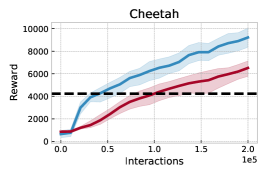
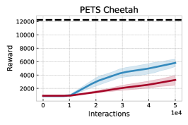
Table 2 shows the results of our method in comparison to POPLIN [77] on the locomotion tasks they consider from Wang et al. [76], POPLIN uses the ground-truth reward for these tasks and learns a model — we learn both. We outperform POPLIN in most of the locomotion tasks, though it has a strong exploration strategy and works exceedingly well in the cheetah environment from PETS [12]. Notably our SAC baseline often also outperforms the SAC baseline reported in Wang and Ba [77]. 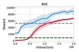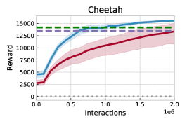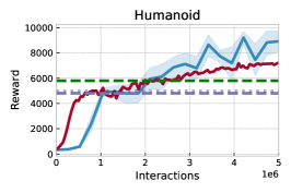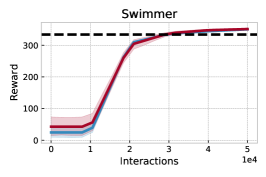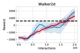We are able to find a policy that generates an optimal action with a single rollout sample rather than the thousands of rollouts POPLIN typically uses and find that setting $H=2$ usually improves upon our SAC baseline ($H=0$). Figure 2 shows our results in comparison to MBPO and STEVE, which evaluate on the MuJoCo tasks in the OpenAI gym [7] that are mostly the standard v2 tasks with early termination and alive bonuses, and with a truncated observation space for the humanoid and ant that discards the inertial measurement units. $\textrm{SAC-SVG}(H)$ consistently matches the best performance and convergence rates across every task and is able to learn a running gait on the humanoid (fig. 1).

Table 2: $\textrm{SAC-SVG}(H)$ excels in the locomotion tasks considered in Wang and Ba [77]. We report the mean evaluation rewards and standard deviations across ten trials.

this paper

	Ant	Hopper	Swimmer	Cheetah	Walker2d	PETS Cheetah
SAC-SVG(1)	3691.00 $\pm$ 1096.77	1594.43 $\pm$ 1689.01	348.40 $\pm$ 8.32	6890.20 $\pm$ 1860.49	-291.54 $\pm$ 659.52	5321.23 $\pm$ 1507.00
SAC-SVG(2)	4473.36 $\pm$ 893.44	2851.90 $\pm$ 361.07	350.22 $\pm$ 3.63	8751.76 $\pm$ 1785.66	447.68 $\pm$ 1139.51	5799.59 $\pm$ 1266.93
SAC-SVG(3)	3833.12 $\pm$ 1418.15	2024.43 $\pm$ 1981.51	340.75 $\pm$ 13.46	9220.39 $\pm$ 1431.77	877.77 $\pm$ 1533.08	5636.93 $\pm$ 2117.52
SAC-SVG(4)	2896.77 $\pm$ 1444.40	2062.16 $\pm$ 1245.33	348.03 $\pm$ 6.35	8175.29 $\pm$ 3226.04	1852.18 $\pm$ 967.61	5807.69 $\pm$ 1008.60
SAC-SVG(5)	3221.66 $\pm$ 1576.25	608.58 $\pm$ 2105.60	340.99 $\pm$ 4.58	6129.02 $\pm$ 3519.98	1309.20 $\pm$ 1281.76	4896.22 $\pm$ 1033.33
SAC-SVG(10)	1389.30 $\pm$ 981.59	-2511.05 $\pm$ 881.26	303.16 $\pm$ 10.57	2477.25 $\pm$ 2596.43	-2328.08 $\pm$ 735.48	4248.25 $\pm$ 802.54
POPLIN-P [77]	2330.1 $\pm$ 320.9	2055.2 $\pm$ 613.8	334.4 $\pm$ 34.2	4235.0 $\pm$ 1133.0	597.0 $\pm$ 478.8	12227.9 $\pm$ 5652.8
SAC* [27]	548.1 $\pm$ 146.6	788.3 $\pm$ 738.2	204.6 $\pm$ 69.3	3459.8 $\pm$ 1326.6	164.5 $\pm$ 1318.6	1745.9 $\pm$ 839.2
SAC (our run)	510.56 $\pm$ 76.38	2180.33 $\pm$ 977.30	351.24 $\pm$ 5.27	6514.83 $\pm$ 1100.61	1265.13 $\pm$ 1317.00	3259.99 $\pm$ 1219.94
PETS* [12]	1165.5 $\pm$ 226.9	114.9 $\pm$ 621.0	326.2 $\pm$ 12.6	2288.4 $\pm$ 1019.0	282.5 $\pm$ 501.6	4204.5 $\pm$ 789.0
METRPO* [44]	282.2 $\pm$ 18.0	1272.5 $\pm$ 500.9	225.5 $\pm$ 104.6	2283.7 $\pm$ 900.4	-1609.3 $\pm$ 657.5	-744.8 $\pm$ 707.1
TD3* [24]	870.1 $\pm$ 283.8	1816.6 $\pm$ 994.8	72.1 $\pm$ 130.9	3015.7 $\pm$ 969.8	-516.4 $\pm$ 812.2	218.9 $\pm$ 593.3
Training Timesteps	200000	200000	50000	200000	200000	50000

*Denotes the baseline results reported in Wang and Ba [77].

Figure 2: $\textrm{SAC-SVG}(H)$ excels in the locomotion tasks considered in Janner et al. [35]. We report the mean evaluation rewards and standard deviations across ten trials.

5.1 Ablations

5.1.1 Model architectures and ensembling

PETS, POPLIN, and MBPO all relied on very similar implementations of bootstrapped ensembles of MLPs to model dynamics. Since we use a different architecture, it is important to consider the impact of the change on the agent’s performance. Simply comparing the reward curves resulting from different model choices does not provide any insight into why some methods perform better than others. In particular, such head-to-head comparisons cannot differentiate between a model’s overall ability to generalize and more subtle interactions with the rest of the agent, such as the effect on exploration.

Figure 3: We compare the multi-step MSE of a 5-component ensemble of MLPs trained on one-step transitions to that of a single recurrent network, trained on multi-step transition sequences. The gap between the holdout curve and the test curve is error due to distribution shift between the train and test distributions. Since the ensemble of MLPs generalizes better in the supervised setting, our performance improvement cannot be attributed to a simple change in model architecture.

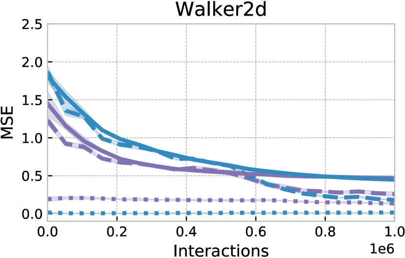
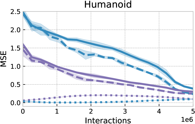
To explore the difference in generalization ability between different architectures, we removed the dependence of the data collection process on the dynamics model by comparing the architectures on an independent episodic replay buffer, generated by a standard model-free SAC trial. By sequentially adding episodes to the model’s training and holdout datasets, retraining the model, and testing on a fixed test split, we isolated the generalization characteristics of the models while simulating the online nature of the RL data-collection process. The results of this experiment are presented in fig. 3. An ensemble of MLPs generalizes better than a single recurrent network of similar capacity. We selected the recurrent network for its amenability to multistep value gradient backpropagation. While we could ensemble our recurrent architecture, we observe that a single model obtains competitive results, and have chosen to prioritize simplicity. Interestingly, even though the single recurrent model overfits much more heavily to the training data, the asymptotic reward of our humanoid agent is significantly higher and qualitatively different than the agent in Janner et al. [35]. Hence it is not clear how well the model needs to generalize, since short-horizon rollouts are typically initiated with states from the replay buffer (i.e. the model’s training data).

5.1.2 Value expansions in the actor and critic

Figure 4: We ablate model rollouts on critic updates and actor updates. Since value learning is particularly sensitive to dynamics model error, on more complex tasks a slightly inaccurate model can halt MVE agent improvement.

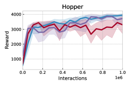
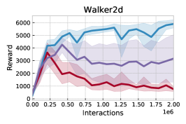
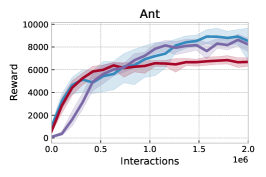
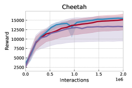
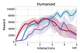
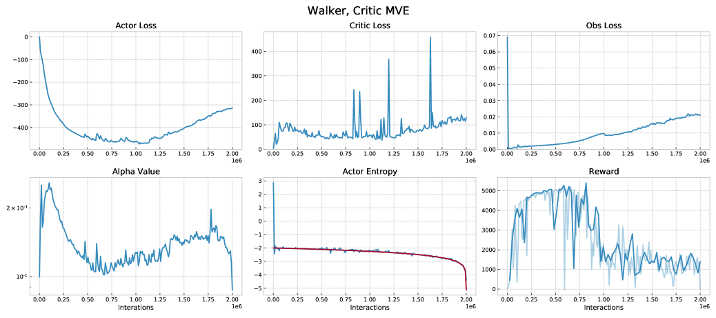
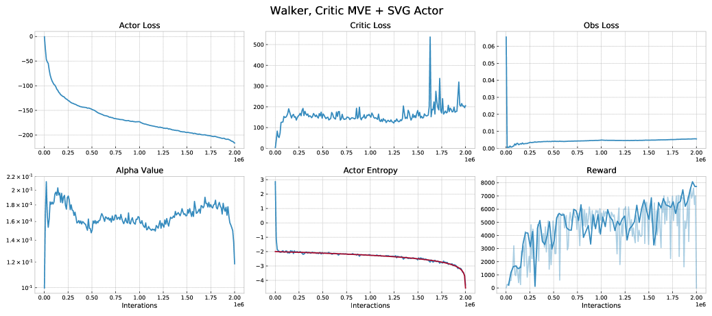
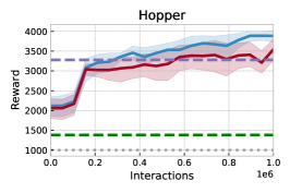
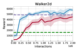
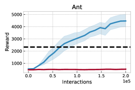
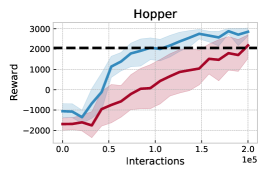
In fig. 4, we consider the effect of introducing the critic MVE update of Feinberg et al. [19] when combined with either the standard model-free SAC actor update or $\textrm{SVG}(H)$. Of particular interest is the first combination, since it bears close resemblance to an ablation performed in Janner et al. [35] on the Hopper environment. In Feinberg et al. [19], both the dynamics model and the actor/critic models are updated with 4 minibatch gradient steps at each timestep. MBPO periodically trained the dynamics model to convergence on the full replay buffer, generated a large batch of fictional transitions, and proceeded to repeatedly update the actor/critic models on those stored transitions.

The contrast between our results and those of the MBPO ablation are instructive. Whereas Janner et al. [35] reported that MVE significantly underperformed MBPO in terms of final reward, even when $H=1$, we find that MVE is competitive on all environments until a certain point in learning, after which performance gradually degrades. A likely explanation lies in the MVE dynamics model update. As the replay buffer grows, the dynamics model update is less likely to sample recent transitions in each minibatch, resulting in a gradual increase in model error (fig. 7). As in fig. 3, the increase in dynamics model error cannot be attributed to the capacity of the model architecture, since the supervised training error on an equivalent replay buffer is significantly lower than the online training error. This observation highlights the impact of model error when the model-generated transitions are used to update the critic, and supports van Hasselt et al. [73] argument that inaccurate parametric forward dynamics models may be particularly detrimental to value learning.

6 Conclusion

$\textrm{SAC-SVG}(H)$ combines the most effective ideas from recent MBRL research, resulting in a simple, robust model-based agent. A few key future directions and applications are in:

1. Policy refinement or semi-amortization as in Marino et al. [49] interprets the policy as solving a model-based control optimization problem and can be combined with differentiable control [53, 3, 58, 2, 17]. Fine-tuning can also be performed at an episode-level as in Nagabandi et al. [52] to adapt the dynamics to the observations in the episode.

2. Constrained MDPs [14, 42, 11, 15, 6], where the model-based value expansion and SVG can guide the agent away from undesirable parts of the state space.

3. Extensions of other model-free algorithms. While we only considered SVG extensions to SAC as presented in Haarnoja et al. [27], similar SVG variations can be added to the policy learning in other model-free methods such as Abdolmaleki et al. [1], Fujimoto et al. [23], Lee et al. [45, 46], Yarats et al. [82].

4. Unsupervised pretraining or self-supervised learning using world models [26, 64, 57, 63, 62] push against the tabula rasa viewpoint of agents starting from zero knowledge about the environment it is interacting with and would allow them to start with a reasonable idea of what primitive skills the system enables them to do.

5. Going beyond the single-agent, single-task, online setting. Some of the core ideas behind model-based value expansion can be applied to more sophisticated settings. In multi-agent settings, an agent can consider short-horizon rollouts of the opponents. In the batch RL setting [22, 43, 79] the short-horizon rollouts can be used to constrain the agent to only considering policies that keep the observations close to the data manifold of observed trajectories.

We thank Alex Terenin, Maximilian Nickel, and Aravind Rajeswaran for insightful discussions and acknowledge the Python community [74, 55] for developing the core set of tools that enabled this work, including PyTorch [56], Hydra [80], Jupyter [40], Matplotlib [33], seaborn [78], numpy [54, 72], pandas [50], and SciPy [36]. This research is supported by an Amazon Research Award, NSF I-DISRE 193471, NIH R01 DA048764-01A1, NSF IIS-1910266, and NSF 1922658 NRT-HDR: FUTURE Foundations, Translation, and Responsibility for Data Science. Samuel Stanton is additionally supported by an NDSEG fellowship from the United States Department of Defense.

Appendix A More experimental details

Algorithm 1 Our combination of SAC and $\textrm{SVG}(H)$. Components of SAC are in colored in black and the model-based SVG components are in purple.

Hyperparameters: #updates $M_{\rm step},M_{\rm seq}$, target network update $\tau$, planning horizon $H$

Models: Actor $\pi_{\theta}$, critic ensemble $Q_{\theta}$, temperature $\alpha$, dynamics $f_{\theta}$, reward $r_{\theta}$, termination $d_{\theta}$

Initialize the replay buffer ${\mathcal{D}}$

for environment step $t=1..T$ do

    Sample $u_{t}\sim\pi(x_{t})$ and execute $u_{t}$ on the system to obtain $(r_{t},x_{t+1},d_{t+1})$ and append it to ${\mathcal{D}}$

    for $M_{\rm step}$ updates do

         ${\mathcal{D}}_{\rm step}\leftarrow\{(x_{s},u_{s},r_{s},x_{s+1},d_{s+1})\}_{s}\sim_{\rm step}{\mathcal{D}}$ $\triangleright$ Sample a batch of single-step transitions

          $\theta_{\pi}\leftarrow\mathrm{grad\_update}(\theta_{\pi},\nabla_{\theta_{\pi}}{\mathcal{J}}_{\pi,\alpha}^{\rm SVG}({\mathcal{D}}_{\rm step}))$ $\triangleright$ Fit the SVG(H) actor with (9)

         $\alpha\leftarrow\mathrm{grad\_update}(\alpha,\nabla_{\alpha}{\mathcal{J}}_{\alpha}({\mathcal{D}}_{\rm step}))$ $\triangleright$ Update the temperature with (8)

         $\theta_{Q}\leftarrow\mathrm{grad\_update}(\theta_{Q},\nabla_{\theta_{Q}}{\mathcal{J}}_{Q}({\mathcal{D}}_{\rm step}))$ $\triangleright$ Fit the critic ensemble with (4)

          $\theta_{r}\leftarrow\mathrm{grad\_update}(\theta_{r},\nabla_{\theta_{r}}{\mathcal{J}}_{r}({\mathcal{D}}_{\rm step}))$ $\triangleright$ Fit the reward model with (11)

          $\theta_{d}\leftarrow\mathrm{grad\_update}(\theta_{d},\nabla_{\theta_{d}}{\mathcal{J}}_{d}({\mathcal{D}}_{\rm step}))$ $\triangleright$ Fit the termination model with (13)

         $\bar{\theta}_{Q}\leftarrow\tau\theta_{Q}+(1-\tau)\bar{\theta}_{Q}$ $\triangleright$ Update the target critic ensemble weights

    end for

    for $M_{\rm seq}$ updates do

         ${\mathcal{D}}_{\rm seq}\leftarrow\{x_{s:s+H}\}_{s}\sim_{\rm seq}{\mathcal{D}}$ $\triangleright$ Sample a batch of multi-step transitions

         $\theta_{f}\leftarrow\mathrm{grad\_update}(\theta_{f},\nabla_{\theta_{f}}{\mathcal{J}}_{f}({\mathcal{D}}_{\rm seq}))$ $\triangleright$ Fit the multi-step dynamics model with (10)

    end for

end for

This section provides more details behind our experiments, including a time-dependent target entropy in sect. A.1, a description of our hyper-parameters in sect. A.2, further analysis and descriptions of a walker experiment in sect. A.3, and full plots of our POPLIN experiments in fig. 5. Algorithm 1 overviews the algorithm describing our combination of SAC and $\textrm{SVG}(H)$.

Figure 5: Results on the environments tasks considered in POPLIN. We run SAC-SVG for ten trials and report the mean and standard deviation of the reward.

A.1 Time-dependent target entropy

Figure 6: Example target entropy decay schedules when training for 1M timesteps with a target entropy starting of $0$ and ending at $-10$.

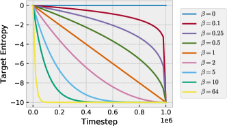
We explicitly decay the policy’s target entropy $\bar{\mathcal{H}}$ rather than keeping it fixed the entire episode as done in vanilla SAC. The target entropy is important for balancing exploration and exploitation and manually decaying it helps control the agent in data-limited settings. This allows us to start the training with a high-entropy policy that we explicitly anneal down to a lower entropy by the end of training. We do this with the exponential decay

$$\bar{H}_{t}=(\bar{H}_{\mathrm{init}}-\bar{H}_{\mathrm{final}})(1-t/T)^{\beta}+\bar{H}_{\mathrm{final}},$$ (14)

where $T$ is the number of training timesteps, $\bar{H}_{\mathrm{init}}$ is the initial target entropy, $\bar{H}_{\mathrm{final}}$ is the final target entropy, and $\beta$ is the decay factor. We plot an example of this in fig. 6.

A.2 Hyper-parameters and random search

We share the hyper-parameters in table 3 between the tasks and only search over the horizon and target entropy values, which we show in table 4. We only perform a hyper-parameter search over the target entropy decay rates for each task, which is important to learn as it impacts how the agent explores in the environment. We found $\textrm{SAC-SVG}(H)$ to be more sensitive to the target entropy decay rate and posit it is important to help the policy interact with the model-based components in the earlier phases of training. We perform a random search over 20 seeds for each task to find a target entropy schedule, where we sample $\bar{H}_{\mathrm{init}}\sim{\rm Cat}(\{1,0,-1,-2\})$, $\bar{H}_{\mathrm{final}}\sim{\rm Cat}\left(\{\bar{H}_{\mathrm{init}},-5\}\cup\{-2^{i}|i\in\{0,\ldots,6\}\}\right)$, and $\gamma\sim{\rm Cat}\left(\{2^{i}|i\in\{0,\ldots,6\}\}\right)$, where ${\rm Cat}(\cdot)$ is a uniform categorical distribution.

Table 3: Shared hyper-parameters for all tasks. SAC’s base hyper-parameters are in black and our $\textrm{SVG}(H)$ extensions are in purple.

Hyper-Parameter	Value
Replay buffer capacity	1M interactions
All optimizers	Adam
Actor and critic LRs	$10^{-4}$
Temperature LR	$5\cdot 10^{-4}$
Init temperature $\alpha_{\rm init}$	0.1
Critic target update rate $\tau$	$5\cdot 10^{-3}$
Critic target update freq	every timestep
Actor update freq	every timestep
Discount $\gamma$	0.99
Single-step updates $N_{step}$	1
Single-step batch size	512
Actor and critic MLPs	2 hidden layers, 512 units
Actor log-std bounds	$[-5,2]$
Reward, term, and dx MLPs	2 hidden layers, 512 units
Dx recurrence	2-layer GRU, 512 units
Reward, term, and dx LRs	$10^{-3}$
Multi-step updates $N_{seq}$	4
Multi-step batch size	1024

Table 4: Task-specific hyper-parameters for the POPLIN (left) and MBPO (right) tasks.

Environment	$H$	$\bar{H}_{\mathrm{init}}$	$\bar{H}_{\mathrm{final}}$	$\beta$
Ant	3	1	-4	0.0625
Hopper	3	1	1	-
Swimmer	3	-2	-16	16
Cheetah	4	0	-4	1
Walker2d	5	1	1	-
PETS Cheetah	5	-2	-4	0.0625

Environment	$\bar{H}_{\mathrm{init}}$	$\bar{H}_{\mathrm{final}}$	$\beta$
Hopper	0	-1	0.5
Walker2d	-2	-3	64
Ant	2	-4	1
Cheetah	-2	-2	-
Humanoid	-1	-1	-

A.3 Walker experiment analysis when doing critic MVE

We provide additional data from selected walker trials that use value expansion on the critic and $\textrm{SVG}(H)$ expansion on the actor behind the summary shown in fig. 4. In MVE trials that perform poorly we can see the model error increase until eventually the agent stops improving. As noted in the previous section, this phenomenon highlights the impact of model error when the model-generated transitions are used to update the critic, and lends credence to the argument of van Hasselt et al. [73], who also suggest that inaccurate parametric forward dynamics models may be particularly detrimental to value learning.

Figure 7: The full details behind the Walker runs when performing critic value expansion with model-free actor updates (top) and critic value expansion with the $\textrm{SVG}(H)$ actor updates (bottom). We find value-expanding in the actor typically leads to more stable behavior.

References

- Abdolmaleki et al. [2018] Abbas Abdolmaleki, Jost Tobias Springenberg, Yuval Tassa, Remi Munos, Nicolas Heess, and Martin Riedmiller. Maximum a posteriori policy optimisation. arXiv preprint arXiv:1806.06920, 2018.
- Agrawal et al. [2019] Akshay Agrawal, Shane Barratt, Stephen Boyd, and Bartolomeo Stellato. Learning convex optimization control policies, 2019.
- Amos et al. [2018] Brandon Amos, Ivan Jimenez, Jacob Sacks, Byron Boots, and J Zico Kolter. Differentiable mpc for end-to-end planning and control. In Advances in Neural Information Processing Systems, pages 8289–8300, 2018.
- Antos et al. [2008] András Antos, Csaba Szepesvári, and Rémi Munos. Fitted q-iteration in continuous action-space mdps. In Advances in neural information processing systems, pages 9–16, 2008.
- Berner et al. [2019] Christopher Berner, Greg Brockman, Brooke Chan, Vicki Cheung, Przemysław Dębiak, Christy Dennison, David Farhi, Quirin Fischer, Shariq Hashme, Chris Hesse, et al. Dota 2 with large scale deep reinforcement learning. arXiv preprint arXiv:1912.06680, 2019.
- Bohez et al. [2019] Steven Bohez, Abbas Abdolmaleki, Michael Neunert, Jonas Buchli, Nicolas Heess, and Raia Hadsell. Value constrained model-free continuous control. arXiv preprint arXiv:1902.04623, 2019.
- Brockman et al. [2016] Greg Brockman, Vicki Cheung, Ludwig Pettersson, Jonas Schneider, John Schulman, Jie Tang, and Wojciech Zaremba. Openai gym. arXiv preprint arXiv:1606.01540, 2016.
- Buckman et al. [2018] Jacob Buckman, Danijar Hafner, George Tucker, Eugene Brevdo, and Honglak Lee. Sample-efficient reinforcement learning with stochastic ensemble value expansion. In Advances in Neural Information Processing Systems, pages 8224–8234, 2018.
- Byravan et al. [2019] Arunkumar Byravan, Jost Tobias Springenberg, Abbas Abdolmaleki, Roland Hafner, Michael Neunert, Thomas Lampe, Noah Siegel, Nicolas Heess, and Martin Riedmiller. Imagined value gradients: Model-based policy optimization with transferable latent dynamics models. arXiv preprint arXiv:1910.04142, 2019.
- Cho et al. [2014] Kyunghyun Cho, Bart Van Merriënboer, Caglar Gulcehre, Dzmitry Bahdanau, Fethi Bougares, Holger Schwenk, and Yoshua Bengio. Learning phrase representations using rnn encoder-decoder for statistical machine translation. arXiv preprint arXiv:1406.1078, 2014.
- Chow et al. [2018] Yinlam Chow, Ofir Nachum, Edgar Duenez-Guzman, and Mohammad Ghavamzadeh. A lyapunov-based approach to safe reinforcement learning. In Advances in neural information processing systems, pages 8092–8101, 2018.
- Chua et al. [2018] Kurtland Chua, Roberto Calandra, Rowan McAllister, and Sergey Levine. Deep reinforcement learning in a handful of trials using probabilistic dynamics models. In Advances in Neural Information Processing Systems, 2018.
- Clavera et al. [2020] Ignasi Clavera, Violet Fu, and Pieter Abbeel. Model-augmented actor-critic: Backpropagating through paths. arXiv preprint arXiv:2005.08068, 2020.
- Dalal et al. [2018] Gal Dalal, Krishnamurthy Dvijotham, Matej Vecerik, Todd Hester, Cosmin Paduraru, and Yuval Tassa. Safe exploration in continuous action spaces. arXiv preprint arXiv:1801.08757, 2018.
- Dean et al. [2019] Sarah Dean, Stephen Tu, Nikolai Matni, and Benjamin Recht. Safely learning to control the constrained linear quadratic regulator. In 2019 American Control Conference (ACC), pages 5582–5588. IEEE, 2019.
- Deisenroth and Rasmussen [2011] Marc Deisenroth and Carl E Rasmussen. Pilco: A model-based and data-efficient approach to policy search. In Proceedings of the 28th International Conference on machine learning (ICML-11), pages 465–472, 2011.
- East et al. [2020] Sebastian East, Marco Gallieri, Jonathan Masci, Jan Koutník, and Mark Cannon. Infinite-horizon differentiable model predictive control. arXiv preprint arXiv:2001.02244, 2020.
- Engstrom et al. [2020] Logan Engstrom, Andrew Ilyas, Shibani Santurkar, Dimitris Tsipras, Firdaus Janoos, Larry Rudolph, and Aleksander Madry. Implementation matters in deep policy gradients: A case study on ppo and trpo. arXiv preprint arXiv:2005.12729, 2020.
- Feinberg et al. [2018] V Feinberg, A Wan, I Stoica, MI Jordan, JE Gonzalez, and S Levine. Model-based value expansion for efficient model-free reinforcement learning. In Proceedings of the 35th International Conference on Machine Learning (ICML 2018), 2018.
- Fischer [2018] Thomas G Fischer. Reinforcement learning in financial markets-a survey. Technical report, FAU Discussion Papers in Economics, 2018.
- Fox et al. [2015] Roy Fox, Ari Pakman, and Naftali Tishby. Taming the noise in reinforcement learning via soft updates. arXiv preprint arXiv:1512.08562, 2015.
- Fujimoto et al. [2018a] Scott Fujimoto, David Meger, and Doina Precup. Off-policy deep reinforcement learning without exploration. CoRR, 2018a.
- Fujimoto et al. [2018b] Scott Fujimoto, Herke Van Hoof, and David Meger. Addressing function approximation error in actor-critic methods. arXiv preprint arXiv:1802.09477, 2018b.
- Fujimoto et al. [2018c] Scott Fujimoto, Herke van Hoof, and David Meger. Addressing function approximation error in actor-critic methods. In Proceedings of the 35th International Conference on Machine Learning, ICML 2018, Stockholmsmässan, Stockholm, Sweden, July 10-15, 2018, 2018c.
- Gu et al. [2016] Shixiang Gu, Timothy Lillicrap, Ilya Sutskever, and Sergey Levine. Continuous deep q-learning with model-based acceleration. In International Conference on Machine Learning, pages 2829–2838, 2016.
- Ha and Schmidhuber [2018] David Ha and Jürgen Schmidhuber. Recurrent world models facilitate policy evolution. In Advances in Neural Information Processing Systems 31. Curran Associates, Inc., 2018.
- Haarnoja et al. [2018] Tuomas Haarnoja, Aurick Zhou, Kristian Hartikainen, George Tucker, Sehoon Ha, Jie Tan, Vikash Kumar, Henry Zhu, Abhishek Gupta, Pieter Abbeel, et al. Soft actor-critic algorithms and applications. arXiv preprint arXiv:1812.05905, 2018.
- Hafner et al. [2019] Danijar Hafner, Timothy Lillicrap, Jimmy Ba, and Mohammad Norouzi. Dream to control: Learning behaviors by latent imagination. arXiv preprint arXiv:1912.01603, 2019.
- Hamrick et al. [2020] Jessica B Hamrick, Abram L Friesen, Feryal Behbahani, Arthur Guez, Fabio Viola, Sims Witherspoon, Thomas Anthony, Lars Buesing, Petar Veličković, and Théophane Weber. On the role of planning in model-based deep reinforcement learning. arXiv preprint arXiv:2011.04021, 2020.
- Hasselt [2010] Hado V Hasselt. Double q-learning. In Advances in neural information processing systems, pages 2613–2621, 2010.
- Heess et al. [2015] Nicolas Heess, Gregory Wayne, David Silver, Timothy Lillicrap, Tom Erez, and Yuval Tassa. Learning continuous control policies by stochastic value gradients. In Advances in Neural Information Processing Systems, pages 2944–2952, 2015.
- Henderson et al. [2018] Peter Henderson, Riashat Islam, Philip Bachman, Joelle Pineau, Doina Precup, and David Meger. Deep reinforcement learning that matters. In Thirty-Second AAAI Conference on Artificial Intelligence, 2018.
- Hunter [2007] John D Hunter. Matplotlib: A 2d graphics environment. Computing in science & engineering, 9(3):90, 2007.
- Islam et al. [2017] Riashat Islam, Peter Henderson, Maziar Gomrokchi, and Doina Precup. Reproducibility of benchmarked deep reinforcement learning tasks for continuous control. arXiv preprint arXiv:1708.04133, 2017.
- Janner et al. [2019] Michael Janner, Justin Fu, Marvin Zhang, and Sergey Levine. When to trust your model: Model-based policy optimization. arXiv preprint arXiv:1906.08253, 2019.
- Jones et al. [2014] Eric Jones, Travis Oliphant, and Pearu Peterson. SciPy: Open source scientific tools for Python. 2014.
- Justesen et al. [2019] Niels Justesen, Philip Bontrager, Julian Togelius, and Sebastian Risi. Deep learning for video game playing. IEEE Transactions on Games, 2019.
- Kaiser et al. [2019] Lukasz Kaiser, Mohammad Babaeizadeh, Piotr Milos, Blazej Osinski, Roy H Campbell, Konrad Czechowski, Dumitru Erhan, Chelsea Finn, Piotr Kozakowski, Sergey Levine, et al. Model-based reinforcement learning for atari. arXiv preprint arXiv:1903.00374, 2019.
- Kiumarsi et al. [2017] Bahare Kiumarsi, Kyriakos G Vamvoudakis, Hamidreza Modares, and Frank L Lewis. Optimal and autonomous control using reinforcement learning: A survey. IEEE transactions on neural networks and learning systems, 29(6):2042–2062, 2017.
- Kluyver et al. [2016] Thomas Kluyver, Benjamin Ragan-Kelley, Fernando Pérez, Brian E Granger, Matthias Bussonnier, Jonathan Frederic, Kyle Kelley, Jessica B Hamrick, Jason Grout, Sylvain Corlay, et al. Jupyter notebooks-a publishing format for reproducible computational workflows. In ELPUB, pages 87–90, 2016.
- Kober et al. [2013] Jens Kober, J Andrew Bagnell, and Jan Peters. Reinforcement learning in robotics: A survey. The International Journal of Robotics Research, 32(11):1238–1274, 2013.
- Koller et al. [2018] Torsten Koller, Felix Berkenkamp, Matteo Turchetta, and Andreas Krause. Learning-based model predictive control for safe exploration. In 2018 IEEE Conference on Decision and Control (CDC), pages 6059–6066. IEEE, 2018.
- Kumar et al. [2019] Aviral Kumar, Justin Fu, Matthew Soh, George Tucker, and Sergey Levine. Stabilizing off-policy q-learning via bootstrapping error reduction. In Advances in Neural Information Processing Systems, pages 11761–11771, 2019.
- Kurutach et al. [2018] Thanard Kurutach, Ignasi Clavera, Yan Duan, Aviv Tamar, and Pieter Abbeel. Model-ensemble trust-region policy optimization. arXiv preprint arXiv:1802.10592, 2018.
- Lee et al. [2019] A. X. Lee, A. Nagabandi, P. Abbeel, and S. Levine. Stochastic latent actor-critic: Deep reinforcement learning with a latent variable model. arXiv e-prints, 2019.
- Lee et al. [2020] Kimin Lee, Michael Laskin, Aravind Srinivas, and Pieter Abbeel. Sunrise: A simple unified framework for ensemble learning in deep reinforcement learning. arXiv preprint arXiv:2007.04938, 2020.
- Levine and Koltun [2013] Sergey Levine and Vladlen Koltun. Guided policy search. In International Conference on Machine Learning, pages 1–9, 2013.
- Lillicrap et al. [2015] Timothy P Lillicrap, Jonathan J Hunt, Alexander Pritzel, Nicolas Heess, Tom Erez, Yuval Tassa, David Silver, and Daan Wierstra. Continuous control with deep reinforcement learning. arXiv preprint arXiv:1509.02971, 2015.
- Marino et al. [2020] Joseph Marino, Alexandre Piché, Alessandro Davide Ialongo, and Yisong Yue. Iterative amortized policy optimization. arXiv preprint arXiv:2010.10670, 2020.
- McKinney [2012] Wes McKinney. Python for data analysis: Data wrangling with Pandas, NumPy, and IPython. " O’Reilly Media, Inc.", 2012.
- Mnih et al. [2015] Volodymyr Mnih, Koray Kavukcuoglu, David Silver, Andrei A Rusu, Joel Veness, Marc G Bellemare, Alex Graves, Martin Riedmiller, Andreas K Fidjeland, Georg Ostrovski, et al. Human-level control through deep reinforcement learning. Nature, 518(7540):529–533, 2015.
- Nagabandi et al. [2018] Anusha Nagabandi, Ignasi Clavera, Simin Liu, Ronald S Fearing, Pieter Abbeel, Sergey Levine, and Chelsea Finn. Learning to adapt in dynamic, real-world environments through meta-reinforcement learning. arXiv preprint arXiv:1803.11347, 2018.
- Okada et al. [2017] Masashi Okada, Luca Rigazio, and Takenobu Aoshima. Path integral networks: End-to-end differentiable optimal control. arXiv preprint arXiv:1706.09597, 2017.
- Oliphant [2006] Travis E Oliphant. A guide to NumPy, volume 1. Trelgol Publishing USA, 2006.
- Oliphant [2007] Travis E Oliphant. Python for scientific computing. Computing in Science & Engineering, 9(3):10–20, 2007.
- Paszke et al. [2019] Adam Paszke, Sam Gross, Francisco Massa, Adam Lerer, James Bradbury, Gregory Chanan, Trevor Killeen, Zeming Lin, Natalia Gimelshein, Luca Antiga, et al. Pytorch: An imperative style, high-performance deep learning library. In Advances in neural information processing systems, pages 8026–8037, 2019.
- Pathak et al. [2019] Deepak Pathak, Dhiraj Gandhi, and Abhinav Gupta. Self-supervised exploration via disagreement. arXiv preprint arXiv:1906.04161, 2019.
- Pereira et al. [2018] Marcus Pereira, David D Fan, Gabriel Nakajima An, and Evangelos Theodorou. Mpc-inspired neural network policies for sequential decision making. arXiv preprint arXiv:1802.05803, 2018.
- Polydoros and Nalpantidis [2017] Athanasios S Polydoros and Lazaros Nalpantidis. Survey of model-based reinforcement learning: Applications on robotics. Journal of Intelligent & Robotic Systems, 86(2):153–173, 2017.
- Puterman [2014] Martin L Puterman. Markov decision processes: discrete stochastic dynamic programming. John Wiley & Sons, 2014.
- Schrittwieser et al. [2020] Julian Schrittwieser, Ioannis Antonoglou, Thomas Hubert, Karen Simonyan, Laurent Sifre, Simon Schmitt, Arthur Guez, Edward Lockhart, Demis Hassabis, Thore Graepel, et al. Mastering atari, go, chess and shogi by planning with a learned model. Nature, 588(7839):604–609, 2020.
- Sekar et al. [2020] Ramanan Sekar, Oleh Rybkin, Kostas Daniilidis, Pieter Abbeel, Danijar Hafner, and Deepak Pathak. Planning to explore via self-supervised world models. arXiv preprint arXiv:2005.05960, 2020.
- Sharma et al. [2020] Archit Sharma, Shane Gu, Sergey Levine, Vikash Kumar, and Karol Hausman. Dynamics-aware unsupervised skill discovery. In Proceeding of the International Conference on Learning Representations (ICLR), Addis Ababa, Ethiopia, pages 26–30, 2020.
- Shyam et al. [2018] Pranav Shyam, Wojciech Jaśkowski, and Faustino Gomez. Model-based active exploration. arXiv preprint arXiv:1810.12162, 2018.
- Sinha et al. [2020] Samarth Sinha, Homanga Bharadhwaj, Aravind Srinivas, and Animesh Garg. D2rl: Deep dense architectures in reinforcement learning. arXiv preprint arXiv:2010.09163, 2020.
- Springenberg et al. [2020] Jost Tobias Springenberg, Nicolas Heess, Daniel Mankowitz, Josh Merel, Arunkumar Byravan, Abbas Abdolmaleki, Jackie Kay, Jonas Degrave, Julian Schrittwieser, Yuval Tassa, et al. Local search for policy iteration in continuous control. arXiv preprint arXiv:2010.05545, 2020.
- Sutton [1990] Richard S Sutton. Integrated architectures for learning, planning, and reacting based on approximating dynamic programming. In Machine learning proceedings 1990, pages 216–224. Elsevier, 1990.
- Sutton and Barto [2018] Richard S Sutton and Andrew G Barto. Reinforcement learning: An introduction. MIT press, 2018.
- Szepesvári [2010] Csaba Szepesvári. Algorithms for reinforcement learning. Synthesis lectures on artificial intelligence and machine learning, 4(1):1–103, 2010.
- Thomas [2014] Philip Thomas. Bias in natural actor-critic algorithms. In International conference on machine learning, pages 441–448, 2014.
- Todorov et al. [2012] Emanuel Todorov, Tom Erez, and Yuval Tassa. Mujoco: A physics engine for model-based control. In 2012 IEEE/RSJ International Conference on Intelligent Robots and Systems, 2012.
- Van Der Walt et al. [2011] Stefan Van Der Walt, S Chris Colbert, and Gael Varoquaux. The numpy array: a structure for efficient numerical computation. Computing in Science & Engineering, 13(2):22, 2011.
- van Hasselt et al. [2019] Hado P van Hasselt, Matteo Hessel, and John Aslanides. When to use parametric models in reinforcement learning? In Advances in Neural Information Processing Systems, pages 14322–14333, 2019.
- Van Rossum and Drake Jr [1995] Guido Van Rossum and Fred L Drake Jr. Python reference manual. Centrum voor Wiskunde en Informatica Amsterdam, 1995.
- Vinyals et al. [2019] Oriol Vinyals, Igor Babuschkin, Wojciech M Czarnecki, Michaël Mathieu, Andrew Dudzik, Junyoung Chung, David H Choi, Richard Powell, Timo Ewalds, Petko Georgiev, et al. Grandmaster level in starcraft ii using multi-agent reinforcement learning. Nature, 575(7782):350–354, 2019.
- Wang et al. [2019] T. Wang, X. Bao, I. Clavera, J. Hoang, Y. Wen, E. Langlois, S. Zhang, G. Zhang, P. Abbeel, and J. Ba. Benchmarking model-based reinforcement learning. arXiv e-prints, 2019.
- Wang and Ba [2019] Tingwu Wang and Jimmy Ba. Exploring model-based planning with policy networks. arXiv preprint arXiv:1906.08649, 2019.
- Waskom et al. [2018] Michael Waskom, Olga Botvinnik, Drew O’Kane, Paul Hobson, Joel Ostblom, Saulius Lukauskas, David C Gemperline, Tom Augspurger, Yaroslav Halchenko, John B. Cole, Jordi Warmenhoven, Julian de Ruiter, Cameron Pye, Stephan Hoyer, Jake Vanderplas, Santi Villalba, Gero Kunter, Eric Quintero, Pete Bachant, Marcel Martin, Kyle Meyer, Alistair Miles, Yoav Ram, Thomas Brunner, Tal Yarkoni, Mike Lee Williams, Constantine Evans, Clark Fitzgerald, Brian, and Adel Qalieh. mwaskom/seaborn: v0.9.0 (july 2018), July 2018. URL https://doi.org/10.5281/zenodo.1313201.
- Wu et al. [2019] Yifan Wu, George Tucker, and Ofir Nachum. Behavior regularized offline reinforcement learning. CoRR, 2019.
- Yadan [2019] Omry Yadan. Hydra - a framework for elegantly configuring complex applications. Github, 2019. URL https://github.com/facebookresearch/hydra.
- Yarats and Kostrikov [2020] Denis Yarats and Ilya Kostrikov. Soft actor-critic (sac) implementation in pytorch. https://github.com/denisyarats/pytorch_sac, 2020.
- Yarats et al. [2019] Denis Yarats, Amy Zhang, Ilya Kostrikov, Brandon Amos, Joelle Pineau, and Rob Fergus. Improving sample efficiency in model-free reinforcement learning from images. arXiv preprint arXiv:1910.01741, 2019.
- Ziebart [2010] Brian D Ziebart. Modeling purposeful adaptive behavior with the principle of maximum causal entropy. 2010.
- Ziebart et al. [2008] Brian D Ziebart, Andrew L Maas, J Andrew Bagnell, and Anind K Dey. Maximum entropy inverse reinforcement learning. In Aaai, volume 8, pages 1433–1438. Chicago, IL, USA, 2008.