A modelling study of hydrodynamical and biogeochemical processes within the California Upwelling System

Abstract

The ROMS modeling system was applied to the California Upwelling System (CalUS) to understand the key hydrodynamic conditions and dynamics of the nitrogen-based ecosystem using the NPZD model proposed by Powell et al. (2006). A new type of sponge layer has been successfully implemented in the ROMS modelling system in order to stabilize the hydrodynamic part of the modeling system when using so-called ”reduced” boundary conditions. The hydrodynamic performance of the model was examined using a tidal analysis based on tidal measurement data, a comparison of the modeled sea surface temperature (SST) with buoy and satellite data, and vertical sections of the currents along the coast and the water temperature. This validation process shows that the hydrodynamic module used in this study can reproduce the basic hydrodynamic and circulation characteristics within the CalUS. The results of the ecosystem model show the characteristic features of upwelling regions as well as the well-known spotty horizontal structures of the zooplankton community. The model thus provides a solid basis for the hydrodynamic and ecological characteristics of the CalUS and enables the ecological model to be expanded into a complex ecological model for investigating the effects of climate change on the ecological balance in the area investigated.

1 Introduction

Eastern boundary upwelling (EBU) system belong to the most productive regions of the word ocean, which is due to the fuelling of the photic zone by cool and nutrient rich water masses from below based on offshore Ekman transport in surface waters. These upwelling regions account for only about 1 % of the global ocean, but produce about 20 % of the global fish catch and are also known to support sea birds and mammals such as whales and seals (see e.g. Kämpf and Chapman (2016) for a general overview of global upwelling systems). The four main eastern boundary systems are those off a) California / Oregon / Washington in the North Pacific, b) Peru and Chile in the South Pacific, c) off northwest Africa and Portugal in the North Atlantic, and d) off South Africa and Namibia in the South Atlantic. Apart from these four major systems, a number of other upwelling systems exist throughout the global ocean, some of which are year-round features, whereas others occur on a seasonal basis (Kämpf and Chapman, 2016).

Understanding the physical and biogeochemical processes in these upwelling systems is of great importance. And coupled modelling systems have been valuable tools in the past to contribute to this understanding. Within this manuscript, we want to focus on the California Upwelling System (CalUS) and have developed a coupled modelling system for that region. In detail, we use a 3D coastal ocean circulation model coupled to a lower trophic level nitrogen-based ecosystem model, which are part of the ROMS modelling system (Regional Ocean Modelling System, see e.g. Haidvogel et al., 2000; Wilkin et al., 2005).

The ROMS modelling system has been applied to the CalUS many times before (see e.g. Gruber et al., 2006; Song et al., 2011; Jacox et al., 2014), in order to study different physical and biogeochemical processes. For example, the strong horizontal nutrient gradients and lateral horizontal transports by filaments and mesoscale eddies, which are characteristic for EBUs, was nicely illustrated (see e.g. Marchesiello et al., 2003; Nagai et al., 2015).

This manuscript describes the application of the ROMS modelling system to the CalUS. The used lower trophic level nitrogen-based ecosystem model is based on the four-component NPZD model by Powell et al. (2006), which itself is mainly based on the studies by Spitz et al. (2003) and Newberger et al. (2003). We show some validation of the physical and biological module.

The interested reader will find a short overview of the California Current System in Section 2. In Section 3, the modelling System is described, and its validation is presented in Section 4. Finally, the new sponge layer type used to stabilize the ROMS modelling system when using so-called reduced boundary conditions is presented and discussed in A.

2 The California Current System

As the hydrography and its variability of the California Current System (CCS) has been described in the past by many authors (see e.g. Hickey, 1979; Lynn and Simpson, 1987; Strub and James, 2000; Centurioni et al., 2008; Checkley and Barth, 2009; Gangopadhyay et al., 2011; Kämpf and Chapman, 2016, and references therein), we only want to give a brief description of the CCS in order to provide the background for evaluating the hydrodynamic model features presented below.

The California Current System consists of different current features with different water mass characteristics due to their source regions, that are located at surface or below surface, and which might show a northward or southward net flow structure (see e.g. Checkley and Barth (2009) Fig. 1 or Gangopadhyay et al. (2011) Fig. 3 for a general overview of the different current features). It extends, in the north, from the Transition Zone (50^∘N, separating the North Pacific and Alaska gyres), where the east-flowing North Pacific Current (also called the West Wind Drift, see e.g. Strub and James, 2000) approaches North America, to subtropical waters off Baja California, Mexico ($\sim$ 15-25^∘N) in the south (Hickey, 1979; Checkley and Barth, 2009). Checkley and Barth (2009) and Gangopadhyay et al. (2011) summarize diverse current features and processes on different spatial and temporal scales that occur in the CCS: wind-driven upwelling, the geostrophically balanced California Current (CC), the coastal jet, the California Undercurrent (CU), Inshore Countercurrent (ICC) (Davidson Current), jets (narrow high-speed flows) in general, squirts (localized energetic off-shelf flows), filaments, mushroom-head vortices, mesoscale and sub-mesoscale eddies, and finally large meanders. When describing the horizontal position of these hydrodynamic features, we follow Lynn and Simpson (1987), who separate the CCS into an offshore oceanic zone ($\approx$ 300 - 1000 km), a near-shore coastal zone ($\approx$ 0 - 200 km) and an intervening transition zone ($\approx$ 200 - 300 km) (this spatial division is also evident in Fig. 1 of Checkley and Barth, 2009). These zones interact with each other by various mechanisms, and their widths are only a rough estimate and are not static.

Concerning the California Current (CC), the classical view depicts a slow and broad current that flows equatorward within about 1000 km of the west coast of North America connecting the eastward North Pacific Current at approximately 50^∘N to the westward North Equatorial Current at approximately 20^∘N (Strub and James, 2000; Checkley and Barth, 2009). It is a year-round, and surface-intensified flow usually in the upper 500 m that carries about 10 Sv (Sverdrup et al., 1942; Checkley and Barth, 2009), and, according to Lynn and Simpson (1987), the main core of the CC is located within the transition zone. However, this picture of the slow and broad current has changed over the last decades (see e.g. Davis, 1985; Huyer et al., 1998; Centurioni et al., 2008; Marchesiello et al., 2003). According to Checkley and Barth (2009) and references therein, the southward flow can be partly organized in form of intense equatorward jets that are embedded within the region of slower southward flow (Mooers and Robinson, 1984; Huyer et al., 1998). The intense jets have widths of 50 - 75 km, speeds in excess of 0.5 m s^-1, comprise up to half of the total CC transport, and are mainly located in or near the transition zone mentioned above. According to Collins et al. (2003) and looking at graphs in Strub and James (2000), the observed California Current jets in and near the transition zone can be seen as the inshore edge of the broader mean seasonal equatorward flow of the California Current. In some cases, these jets can be traced back to coastal upwelling jets that separate from the coast, merge offshore (to about 130^∘W) to become a free, open-ocean jet that maintains its identity as the CC core during spring and summer (Barth et al., 2000; Strub and James, 2000; Gangopadhyay et al., 2011).

The near-shore coastal zone and the transition zone show a very complex dynamic, which changes during the year, and with more mesoscale features present in late summer to early fall (e.g. Strub and James, 2000). Within these zones, the upwelling regions, the coastal jet, the California Undercurrent (CU), as well as the Inshore Countercurrent (ICC) are located (Checkley and Barth, 2009). It is the source region of coastal and westward propagating cyclonic and anticyclonic mesoscale eddies (Kurian et al., 2011) and it is the region with all those smaller-scales, high-energetic features like those filaments mentioned above. In addition, within the coastal zone, there exist some frequent standing eddies, like the counterclockwise Southern California eddy located south of Point Conception (Checkley and Barth, 2009), a counterclockwise eddy off San Francisco and about half the distance to Point Conception (Hickey, 1979), eddies near Point Arena, and the Cape Mendocino eddy (Hayward and Mantyla, 1990).

The coastal jet is generated in geostrophic balance due to both a drop in coastal sea level and the presence of the cold water front near the coast (Checkley and Barth, 2009), which generates a strong, equatorward coastal upwelling jet with speeds of up to 1 m s^-1. According to the thermal-wind relation, the coastal upwelling jet is vertically sheared, with strongest currents near the surface, because temperature, salinity and, hence, density vary in the cross-shelf direction. The jet is also horizontally sheared and fastest near the strongest cross-shelf density difference, i.e. the coastal upwelling front (Checkley and Barth, 2009). Interactions of the alongshore flow with coastal and bottom bathymetric features (capes, banks, canyons), in combination with hydrodynamic instability, also leads to intense alongshore variability e.g. visible in transient and even persistent meanders and eddies especially from spring to early fall (Strub and James, 2000; Centurioni et al., 2008; Checkley and Barth, 2009; Drake et al., 2011).

Within the coastal zone of the CCS, two narrow poleward flowing boundary currents are found. These currents, the Inshore Countercurrent (ICC) and the California Undercurrent (CU), are distinguished from each other by their water mass characteristics, their vertical location, and their temporal presence during the year (Collins et al., 2000).

The CU appears as a subsurface maximum of flow between 100 and 250 m depth over the continental slope and transports warm, saline equatorial waters (Chelton, 1984; Lynn and Simpson, 1987; Hickey, 1998). It is considered to originate in the eastern equatorial Pacific and to flow poleward along the North American coast (Sverdrup et al., 1942; Lynn and Simpson, 1987). Thus, the CU can be seen as an example of poleward undercurrents also present in other major ocean basins, which are usually found over the continental slope and which have typical alongshore speeds of 0.1 - 0.3 m s^-1 and a depth range of 100 - 300 m (Pierce et al., 2000). In the mean, the main core of the CU is located at 250 m depth near the continental slope and it does not extend beyond 100 km from the coast, although there is some seasonal variability of the height and strength (mean $\approx$ 5 - 10 cm s^-1) of the core (Lynn and Simpson, 1987; Collins et al., 1996). In detail, the CU has been observed at locations ranging from Baja California to Vancouver Island (Hickey, 1998), and shipboard surveys along the West Coast of the U.S. show poleward flow over the upper slope at all latitudes (Pierce et al., 1996; Collins et al., 2000).

According to Collins et al. (2000), the ICC has been reported as a seasonal flow, appearing in fall and winter (Reid Jr. and Schwartzlose, 1962; Lynn and Simpson, 1987). It is found over both the shelf and slope and transports shallow, upper ocean waters, which mainly are derived from CC waters with some modification by coastal processes. North of Point Conception, the ICC is sometimes called the Davidson Current or the Davidson Inshore Current (Reid Jr. and Schwartzlose, 1962; Hickey, 1979).

3 Description of the coupled modelling system

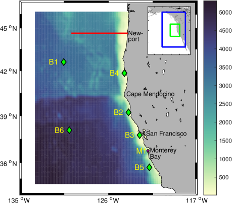
Figure 1: The model area of the 3D modelling system applied to the CalUS. The small panel top right depicts the extent of the parent grid (blue box) and the one-way nested child grid (green box), whose bathymetry is depicted within the larger panel. The symbols B1 - B6 denote the NDBC buoys (used for temperature validation). The red line denotes the position of the Newport transect. Finally, the magenta symbol M1 denotes the position of the M1 buoy of Monterey Bay Aquarium Research Institute (MBARI).

For studying the CalUS, we decided to use the ROMS modelling system (Regional Ocean Modelling System, see e.g. Haidvogel et al., 2000; Wilkin et al., 2005), as it has been applied to this study region many times before.
Here, within this modelling system a 3D coastal ocean circulation model is coupled to a lower trophic level nitrogen-based ecosystem model. In the following we will describe the two modules separately.

3.1 Description of the hydrodynamic module

The hydrodynamic component is built using an online one-way nested system (see model domains in Fig. 1 ) with the coarser parent grid having a horizontal resolution of about 15 km and the nested child grid having a resolution of about 5 km, which corresponds to a three-times nesting refinement. In the vertical, 30 layers of terrain-following S-coordinates are used with a strong refinement near the sea surface to resolve the upper 500 m of the water column and a smaller one near the sea floor (see the corresponding parameters in Tab. 1). To capture subgrid-scale vertical turbulence, a k-kl variant of the Generic Length Scale (GLS) turbulence scheme (Umlauf and Burchard, 2003; Warner et al., 2005) is chosen for estimating vertical mixing coefficients for the hydrodynamic and the biological module, whereas for the horizontal mixing of momentum and active/passive tracers harmonic diffusion with constant turbulent diffusivities is used (see Tab. 1). To deal with the turbulent vertical flux of horizontal momentum within the bottom boundary layer a quadratic bottom friction is selected.

In order to reduce the model spinup-time, initial conditions of free-surface elevation, horizontal water velocities, temperature and salinity for January 2012 are taken from the 1/12 degree global HYCOM + NCODA reanalysis data (HYbrid Coordinate Ocean Model, see e.g. Bleck, 2002; Chassignet et al., 2006). This also means that there is a sufficient amount of turbulence already present at the beginning of the model simulation, which does not have to be built over a spinup process of several years as e.g. described by Marchesiello et al. (2003).

Hydrodynamic open-boundary conditions for the larger parent grid are obtained from two different data sources. In order to include tidal effects into the modelling system, tidal-harmonic constants are provided using the OSU Tidal Data Prediction Software together with the OTIS Regional Tidal Solutions dataset ’PO2009’ for the Pacific Ocean (Egbert and Erofeeva, 2002). In order to obtain an estimate of the true free-surface along the open boundary (tidal + mean background), free-surface elevation model data from the HYCOM + NCODA reanalysis are added to the obtained tidal signal. The vertical-mean horizontal velocities are obtained via the ’reduced’ boundary condition type from the prescribed (’clamped’) free-surface elevation. However, as it is well known that the ROMS modelling system might face some problems at open boundaries when using these kind of ’reduced’ boundary conditions, a new sponge-layer type is implemented into the ROMS model code to stabilize the model along the open boundaries. The working mechanism of this new sponge layer is explained in more detail within A. The three-dimensional horizontal velocities are ’nudged’ to velocity data obtained from the 1/12 degree global HYCOM + NCODA reanalysis data. With using these HYCOM + NCODA reanalysis data sets, the parent model domain is included into the large-scale hydrodynamic circulation of the Pacific Ocean.

Table 1: Model parameters used for the hydrodynamic module of the 3D coupled modelling system

General parameters:
Number of vertical layers	30
S-coordinate transformation equation	2
S-coordinate stretching function	4
S-coordinate surface control parameter	7.0
S-coordinate bottom control parameter	0.5
Quadratic bottom drag coefficient.	0.0025
3D velocity nudging time scale	1.0 d
Tracer nudging time scale	1.0 d
Factor outflow/inflow nudging	10
Parent grid:
External/barotropic time step	1.5 s
Internal/baroclinic time step	30 s
Horizontal resolution	$\approx$ 15 km
Horiz. turbulent viscosity	300 m2 s-1
Horiz. turbulent tracer diffusivity	300 m2 s-1
Child grid:
External/barotropic time step	0.5 s
Internal/baroclinic time step	10 s
Horizontal resolution	$\approx$ 5 km
Horiz. turbulent viscosity	100 m2 s-1
Horiz. turbulent tracer diffusivity	100 m2 s-1

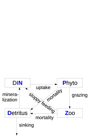
Figure 2: Schematic of the considered biological model after Powell et al. (2006): dissolved inorganic nitrogen (N), particulate nitrogen (detritus: D), phototrophic phytoplankton (P), and herbivorous zooplankton (Z).

The atmospheric forcing (wind speed, air temperature, precipitation, sea-level pressure, total cloud cover and air humidity) is based on 3-hourly ECMWF/ERA5 (2017) reanalysis data with a spatial resolution of about 0.28 degree. Time-varying river runoff data for the year 2012 from USGS, USA, is also included for the following larger rivers: Stikine River (Alaska), Columbia River (Oregon / Washington), Rogue River (Oregon), Klamath River (Oregon / California), Eel River (California), Sacramento River (California), San Joaquin River (California). For each river, its discharge and contribution to salinity has been considered, whereas coastal temperatures and state variables of the biological module are not affected by river runoff.

3.2 Description of the biological module

The Powell et al. (2006) four-component NPZD model, which itself is mainly based on the studies by Spitz et al. (2003) and Newberger et al. (2003), is used as a simple model with sufficient complexity to investigate biogeochemical conversion rates under the influence of turbulent transport processes. The model parameters are mainly taken as described within these articles (with one exception, see below). Therefore, we skip a very detailed validation of the biological model. Within this nitrogen-based trophic module, total nitrogen is partitioned between dissolved inorganic nitrogen (N), particulate organic nitrogen (detritus: D), phototrophic phytoplankton (P), and herbivorous zooplankton (Z).

The dynamics of each of these four components and their interactions are illustrated in Fig. 2 and can be described via a transport-reaction equation of the form:

$$\frac{\partial C}{\partial t}+\nabla\cdot(\boldsymbol{v}C)=\nabla_{h}\cdot(D_{h}\nabla_{h}C)+\frac{\textstyle\partial}{\textstyle\partial z}\left(D_{v}\frac{\partial C}{\partial z}\right)+R$$ (1)

where $\nabla$ denotes the nabla-operator, $\boldsymbol{v}$ the water velocity ($\boldsymbol{v}=(u,v,w)$), $D_{h}$ the horizontal eddy diffusion coefficient, $D_{v}$ the vertical eddy diffusion coefficient, and finally, $R$ the net conversion rate for each species.

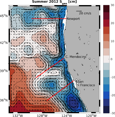
Figure 3: The contour plot denotes the anomaly (the spatial mean has been subtracted) of the summer-mean modified geostrophic stream function $S_{geo}$ after Eq. (9) in 100 m depth, whereas the summer mean Eulerian horizontal velocities at 100 m are denoted by the black arrows. The red lines mark the location of the vertical transects, for which normal velocities and temperatures are plotted within Fig. 4.

In detail, the net biological conversion rates for each species are (for more details see Powell et al., 2006):

$$R_{N} = \delta D+\gamma_{n}GZ-UP$$ (2)

$$R_{P} = UP-GZ-\sigma_{d}P$$ (3)

$$R_{Z} = (1-\gamma_{n})GZ-\zeta_{d}Z$$ (4)

$$R_{D} = \sigma_{d}P+\zeta_{d}Z-\delta D~{}~{}+w_{d}\frac{\partial D}{\partial z}$$ (5)

The detritus rate term $R_{D}$ is augmented by the detritus sinking rate (the last term on the right in Eq. 5), which is actually not a biological conversion term. Furthermore, the following definitions are used:

$$G := R_{m}(1-e^{-\Lambda P})$$ (6)

$$U := \frac{\textstyle V_{m}N}{\textstyle k_{U}+N}\frac{\textstyle\alpha I}{\textstyle\sqrt{V_{m}^{2}+\alpha^{2}I^{2}}}$$ (7)

$$I := I_{0}~{}par~{}exp\left(-k_{z}z-k_{p}\int_{0}^{z}P(z^{\prime})dz^{\prime}\right)$$ (8)

Light attenuation is modelled by Eq. (8), where $z$ denotes the (positive) vertical distance between the sea surface and the position within the water column, $I_{0}$ the variable sea-surface short wave radiation flux, and $par$ the fraction of light that is available for photosynthesis (see e.g. Fennel et al., 2006). The parameters of this NPZD-model are mainly identical to the values used in Powell et al. (2006) and are listed in Tab. 2. However, the parameters of grazing by zooplankton upon phytoplankton have been changed according to Fiechter et al. (2009), as this leads to a larger mortality of phytoplankton due to grazing, which is more realistic for the CalUS (personal communication with Jerome Fiechter).

Figure 4: Horizontal normal current velocity ([m s^-1]) (panels a) - c)) and potential temperature ([^oC]) (panels d) - f)) on the vertical sections marked by the red lines in Fig. 3. Panel a) and d) correspond to the Newport transect, panel b) and e) to CalCOFI line 46.7 starting at Cape Mendocino, and panel c) and f) belong to CalCOFI line 60 starting at San Francisco. Normal velocities in northward direction are denoted by positive (red) values.

Table 2: Model parameters used for the biological module of the coupled 3D modelling system (mainly identical with Powell et al., 2006; Spitz et al., 2003).

Parameter Name	Symbol	Value
Light extinction coeff.	$k_{z}$	0.067 m-1
Self-shading coeff.	$k_{p}$	0.0095 (m $\mu$M-N)-1
Initial slope of P-I curve	$\alpha$	0.025 m2W-1
PAR-fraction	$par$	0.43
Phyto. max. uptake rate	$V_{m}$	1.5 d-1
Uptake half saturation	$k_{U}$	1.0 $\mu$M-N
Phyto. senescence	$\sigma_{d}$	0.1 d-1
Zoop. grazing rate	$R_{m}$	0.65 d-1
Ivlev constant	$\Lambda$	0.84 $\mu$M-N-1
Excretion efficiency	$\gamma_{n}$	0.3
Zoop. mortality	$\zeta_{d}$	0.145 d-1
Remineralization	$\delta$	1.03 d-1
Detrital sinking rate	$w_{d}$	8.0 m d-1

At the open boundaries of the model domain, a nudging method is used to force the biological variables to prescribed values. Apart from the DIN pool, all other biological variables are forced to zero for all times and all depth levels. However, dissolved inorganic nitrogen (DIN) is set according to the depth-dependent annual-mean NO${}_{3}^{-}$ concentration obtained from the Levitus data set (Levitus, 1982). The initial conditions are set to a value of 1.0 mmol-N m^-3 for all variables apart from the nitrogen pool, which is set to 17.0 mmol-N m^-3. So, although DIN also includes other N-species like nitrite or amonium, the boundary and initial conditions were mainly set to nitrate based numbers.

4 ’Validation’ of the modelling system

After this technical description of the two coupled modules, we want to demonstrate that the modelling system at hand provides a sufficient first representation of the CalUS without reproducing all hydrodynamic and biogeochemical features of the CalUS.

4.1 Validation of the hydrodynamic module

Within this part, the hydrodynamic module is to be validated by means of temperature data, data of free-surface elevation, and current velocity.

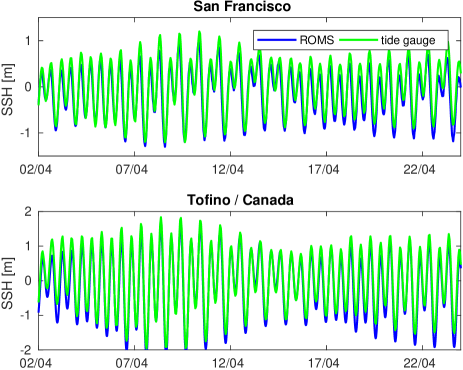
Figure 5: Comparison of modelled sea surface height (SSH) with tide gauge data at Fort Point, San Francisco, and Tofino (Vancouver Island, Canada) over a time-period of two weeks in April 2012.

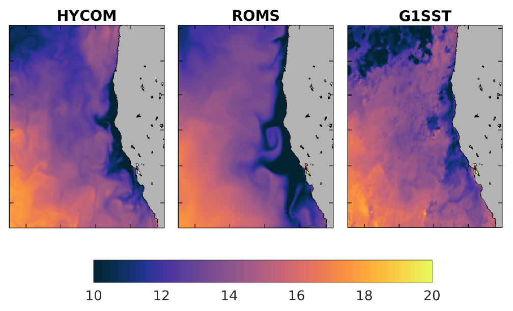
Figure 6: SST at 16 June 2012 obtained from the 1/12 degree global HYCOM + NCODA reanalysis data (left), the hydrodynamic model component of the ROMS modelling system presented in this study (middle), and finally from L4-G1SST satellite data (left).

Current Velocities

First, we want to demonstrate that the model captures the main features of the horizontal circulation within the CCS as described above. As an example, Fig. 3 depicts the summer mean horizontal Eulerian velocity in 100 m depth. In addition, this figure also depicts the contour lines of the anomaly (the spatial mean has been subtracted) of the 2012 summer-mean modified dynamic height:

$$S_{geo}(x,y,z):=\zeta(x,y)+\frac{\textstyle 1}{\textstyle\rho_{0}}\int_{z}^{\zeta}\rho_{ano}(x,y,z^{\prime})dz^{\prime}$$ (9)

Here, $\zeta$ denotes summer-mean sea surface height, $\rho_{0}$ = 1000 kg/m³, $\rho_{ano}$ the density anomaly to 1000 kg/m³ obtained from the summer mean distribution of potential temperature and salinity. As $gS_{geo}/f$ (with $g$ the gravitational acceleration, $f$ the Coriolis parameter) is a geostrophic streamfunction, $S_{geo}$ can be considered as some kind of scaled geostrophic streamfunction, whose contour lines should also be parallel to the geostrophic velocity.

As is evident from Fig. 3, the mean horizontal current velocities are more or less parallel to the streamlines, which is due to the validity of the geostrophic approximation. This picture shows the drop of $S_{geo}$ towards the coast; and the resulting coastal jet mentioned above is clearly visible (especially between Newport and Cape Mendocino). Similar to observations, this jet shows strong meandering, and separates from the coast south of Cape Mendocino as indicated in Fig. 3. of Gangopadhyay et al. (2011). While separating from the coast near Cape Mendocino, the coastal jet seems to split into two branches: one moving offshore, one flowing further near the coast. Also similar with this figure, within the south-west corner of Fig. 3, meanders and jets of the broader and slower CC seem to be visible. In addition, there are also some strong closed contours of the summer mean $S_{geo}$, that might indicate standing eddies within that region. Some of them might corresponds to mentioned features within the literature, as the one south of San Francisco near $36$ N, that might correspond to the San Francisco eddy mentioned in Hickey (1979); likewise the smaller one near Point Arena (near 39 N) mentioned in Hayward and Mantyla (1990).

The mentioned hydrodynamic features are also visible on vertical sections of the horizontal current velocity depicted in Fig. 4, and the positions of these transects of 450 km length are marked by the red lines in Fig. 3. The northern most transect is chosen according to the transect presented in Powell et al. (2006). The two southern lines are chosen after the California Cooperative Fisheries Investigations (CalCOFI) sampling grid. The line starting at Cape Mendocino corresponds to CalCOFI transect with line coordinate 46.7, whereas the southern most line starting at San Francisco corresponds to line coordinate 60. Within a 100 km band close to the coast, the coastal jet is clearly visible in Fig. 4 a) and c). Near Cape Mendocino, due to a meander, the jet has moved more offshore and is visible 200 km from the coast. From this figure, the vertical extent of the main core of the coastal jet is clearly visible to be within the upper 200 m. Furthermore, on all three transects, the California Undercurrent (CU) is visible as the red band near the continental slope with its core to be between 400 - 200 m. However, the CU reaches upwards to 100 m, such that its northward flow velocity is also visible by the northward pointing velocity vectors close to the coast in Fig. 3.

Table 3: Results of the tidal analysis for year 2012 obtained via the T-tide software package (Pawlowicz et al., 2002) at San Francisco and Tofino (Vancouver Island, Canada) tide-gauge stations. The phase difference is obtained by subtracting the phase value of the modelled data from the phase value of the measured data. So, a negative phase difference denotes the model lagging behind the data.

	San Francisco		Tofino
	data	model	data	model
$M_{2}$ amp. [m]	0.57	0.52	0.97	0.96
$M_{2}$ $\Delta\phi$ [∘]	15.05		-0.50
$M_{2}$ $\Delta\phi$ [min]	31.15		-1.04
$S_{2}$ amp. [m]	0.13	0.12	0.28	0.29
$S_{2}$ $\Delta\phi$ [∘]	10.0		-3.72
$S_{2}$ $\Delta\phi$ [min]	19.99		-7.43
$K_{1}$ amp. [m]	0.37	0.41	0.39	0.49
$K_{1}$ $\Delta\phi$ [∘]	8.94		6.57
$K_{1}$ $\Delta\phi$ [min]	35.66		26.20
$O_{1}$ amp. [m]	0.23	0.26	0.24	0.31
$O_{1}$ $\Delta\phi$ [∘]	8.07		7.24
$O_{1}$ $\Delta\phi$ [min]	34.72		31.15

Sea Surface Height (SSH)

As the tides quite significantly contribute to the short-term variability, we want to pay some attention to their representation within the model. As the model is forced along the open boundaries by tidal elevations as described above (here, model errors are only due to the errors within the forcing data), it might be questionable if the (tidal) fluctuations of SSH in the central part of the model domain are of the right order. Therefore, tide gauge data of two stations located in the central area of the model domain have been considered for model validation: from Tofino (Vancouver Island, Canada) within the coarser grid, and from San Francisco (Fort Point) within the finer child grid. As a first inspection, SSH time series for a two-weeks period in April 2012 are depicted in Fig. 5. Although not matching perfectly, it is evident from this figure that the tides are represented appropriately with respect to amplitude and phase at these two tide gauge stations. This is further confirmed by using a Taylor diagram analysis (see Fig. 8) for the total year 2012, which shows the good agreement in terms of standard deviation and correlation. In addition, the harmonic analysis (using the T-tide software package of Pawlowicz et al. (2002)) presented in Tab. 3 shows a satisfactory agreement of the tidal amplitudes of the harmonics M2, S2, O1, and K1 for both tide gauge stations. However, there is some phase lag in the order of some minutes of the M2 and S2 tide in San Francisco, which might be due to small errors in tidal wave propagation. In the end, this validation process demonstrates that the tidal dynamics in the CalUS is represented to the right order of magnitude within the hydrodynamic module at hand.

Water Temperatures

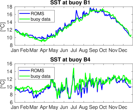
Figure 7: Comparison of modelled (blue line) and measured (green line) sea surface temperature (SST) at buoys B1 and B4 for the year 2012 (for the location of these buoys, please see Fig. 1).

As signatures of upwelling processes are usually visible as specific features of sea surface temperature, we compare time series of modelled and measured SST at different sites within the CalUS, for which buoy data have been available from the NDBC. The locations of these buoys are shown in Fig. 1 and are denoted by symbols B1 - B6, which correspond to the following buoy numbers: B1 - 46002; B2 - 46014 ; B3 - 46026 ; B4 - 46027; B5 - 46028; B6 - 46059.

Fig. 7 depicts the 2012 time series of SST at two buoy sites: one close to the coast (B4) and one more offshore (B1). This figure demonstrates that the model captures the long-term evolution of the SST quite well. It even reproduces the timing and strength of some upwelling events in May and June 2012, which can be seen from the lower panel in Fig. 7. However, is is also visible from the time series of the near-shore site that the model might overestimate the strength of the upwelling process a bit, which could explain the underestimation of the near-shore SST. In addition, the SST comparisons for the other buoy sites are depicted within the Taylor diagram in Fig. 8, from which it is evident that the SST dynamics is captured by the model in a sufficient manner.

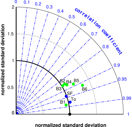
Figure 8: Taylor diagram for validation of modelled sea surface temperature at buoys B1 - B6 (for the location of these buoys, please see Fig. 1) and SSH at tide gauge stations located in San Francisco (SF) and Tofino (To) (Vancouver Island, Canada).

This impression of a slight overestimation of the upwelling process can also been reasoned from Fig. 6, which shows a spatial plot of modelled SST for 16 June 2012 together with SST fields obtained from the HYCOM model and satellite data. Although the position and extent of the upwelling region are quite similar to those features within the HYCOM data and the L4-G1SST satellite data, our model seems to overestimate the upwelling process in that time period to some extent, which is evident from the colder SST values near the coast. However, looking at special features of SST at that day, the model clearly shows filaments as well as mushroom-like and eddy structures due to the upwelling process as mentioned above.

In addition, the near-shore upwelling of colder subsurface waters can also be seen on the vertical CalCOFI sections depicted in Fig. 4 d) - f), which are comparable to vertical temperature sections shown in Marchesiello et al. (2003) or Chenillat et al. (2013).

4.2 ’Validation’ of the biological module

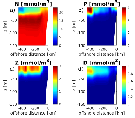
Figure 9: Monthly mean values for May 2012 of the four species of the biological model on the vertical transect near Newport. The location of this transect is depicted within Fig. 1.

To illustrate the performance of the biological module, monthly mean values of dissolved inorganic nitrogen (DIN), phytoplankton and zooplankton are plotted along the Newport transect (similar to Powell et al., 2006, red line in Fig. 1) for May 2012 in Fig. 9. The upwelling of DIN-rich water mass is visible at the coast in panel Fig. 9a, as well as the DIN consumption within the euphotic zone by growing phytoplankton. The growing of zooplankton is visible in panel Fig. 9c, and the remineralization of detritus to DIN is evident from the increase of nutrients below the euphotic zone within the depth-interval between 50 - 100 m in Fig. 9a.

The interaction and the temporal succession of the N-species is also visible within a temporal snapshot of near-surface distributions of the N-species depicted in Fig. 10. This figure shows the horizontal mesoscale structure of the biological variables, which is similar to the structures depicted in Powell et al. (2006), and which also shows an increase in nutrients towards the coast due to the prevailing upwelling dynamics. As an example, within the south-western region of the four panels of this figure, a stretched structure is visible as a depletion of N, which is also present as a build-up within the other panels for P, Z and D. Thus the temporal succession of nitrogen though the four pools is visible.

What is also visible within these horizontal distributions, is the patchy structure of the zooplankton species that is described e.g. in Messié and Chavez (2017). Messié and Chavez (2017) and Fiechter et al. (2020) investigate the formation and occurrence of zooplankton hotspots within the CalUS. They attribute their formation and distribution to regions of coastal nutrient upwelling as well as converging and diverging surface currents. The simple NPZD model at hand shows, to some extent, a similar behaviour as depicted in Fig. 11. Within that figure, the temporal evolution a zooplankton patch near Monterey Bay (denoted as MB within that figure) is shown over a time period of nearly two weeks in June 2012. The simultaneous generation of zooplankton from phytoplankton within an upwelling centre as well as the horizontal transport of zooplankton within a narrow stripe to offshore locations is visible from this figure.

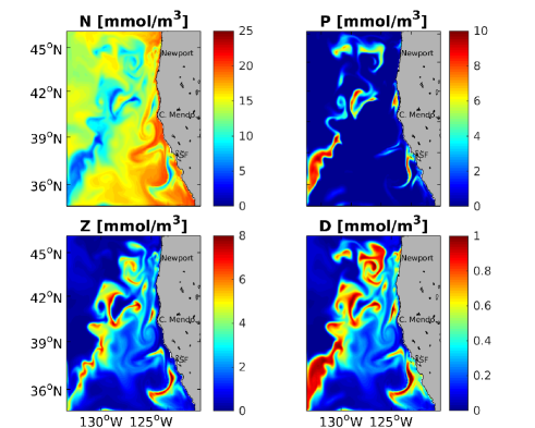
Figure 10: Exemplary horizontal distributions of the biological module at 16 June 2012 in a water depth of 15 m below sea surface.

In order to investigate and validate the temporal dynamics of this simple NPZD model, modelled near-surface DIN concentrations are compared to measured nitrate values at a long-term time series station in Monterey Bay (M1 buoy, see Fig. 1 for the position of this buoy) (Sakamoto et al., 2017; Chavez et al., 2017). Concerning the origin of upwelled water masses, Monterey Bay is mainly influenced by the upwelling center off Año Nuevo (to the north of the bay), from which cold and nutrient-rich water enters Monterey Bay (see e.g. Chavez et al., 2017), although upwelling and/or mixing occurs along the entire region from Año Nuevo to Point Sur. Due to its wind-protection capabilities, its slower circulation and a warm and stable mixed layer, Monterey Bay is a classical upwelling shadow environment that foster dense phytoplankton blooms (Chavez et al., 2017).

As mentioned above, DIN includes more N-species apart from nitrate, such that a direct comparison of nitrate and DIN is problematic, However, the DIN is initialized and set at open boundaries to the order of long-term nitrate concentrations. Therefore, the DIN within this manuscript is of similar magnitude as nitrate. According to Chavez et al. (2017) the nitrate concentration at M1 buoy at the entrance of Monterey Bay is strongly influenced by coastal upwelling of deep nutrient rich waters. Riverine nitrate input is negligible at that site in general and only of some importance during winter months (Sakamoto et al., 2017). The long-term (1988 - 2016) climatological nitrate concentration shows a peak due to coastal upwelling during March and July (Chavez et al., 2017), which is to some extent visible for the year 2012 in Fig. 12 (see green line in upper panel). It is evident from this figure that the modelled nitrate concentration (blue line in upper panel) is of similar magnitude. However, it is also evident that the two time series (modelled and measured) do not match. As an example, the modelled time series depicts some peak at the beginning of August 2012, whereas the measured nitrate data show a falling trend with low absolute values.

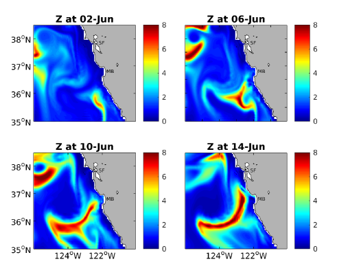
Figure 11: Exemplary horizontal evolution of a zooplankton [mmol/m³] patch in a depth of 15 m below sea surface in the first half June 2012.

In the lower panel of Fig. 12, the modelled (blue line) and measured (green line) SST is depicted, which shows that the overall trend and the right order of magnitude is captured by the model. However, some the short-term fluctuations are not always captured by the model, as can e.g. be seen in mid-May as well as at the beginning of July, when some cooler (an likely upwelling) events are missed by the model.

In order get some idea, what causes these differences, we also compared the SST at this site, which seems to be a good indicator of upwelling waters. According to Sakamoto et al. (2017), as a first approximation, the nitrate concentration (mmol/m³) can be estimated from sea surface temperature (SST, ^oC) by a simple linear regression model (correlation coefficient $r^{2}$ = 0.59) of the form:

$$\text{NO}_{3}^{-}=-2.82\times\text{SST}+43.59$$ (10)

Thus, the top panel also shows the SST-based estimated nitrate concentrations using the modelled (cyan line) and measured (red line) sea surface temperature at buoy M1.

It is evident that the model seems to capture an upwelling event with the largest measured nitrate concentration at the end of May, which is visible in all the four nitrate curves. However, the model shows high measured nitrate concentration at the beginning of July and end of July, which only partially seem to be related to modelled upwelling events. Whereas the event at the beginning of July shows some modelled upwelling signature (the cyan curve shows a small peak), the high nitrate concentration at the end of July / beginning of August has no upwelling counterpart.

The reason for the occasional overestimation of the modelled nitrate data might be due to the initialization of the nitrate concentration within the model domain, which also puts hight nutrient loads in the upper waters of the euphotic zone which is evident from Fig. 9, which shows nutrient concentration of about 15 mmol/m³ in offshore waters. Therefore, in the model, in addition to upwelling of nutrients from below, horizontal currents could transport nutrients to buoy M1, which might explain the nitrate peaks outside the upwelling season. Alternatively, the temporal dynamics of the uncoupled (i.e. without any spatial transports) NPZD model could be visible on this figure.

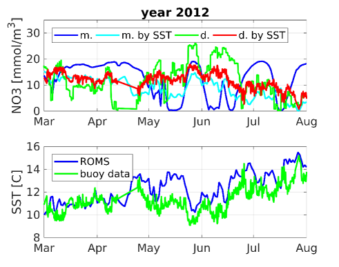
Figure 12: Time series of modelled and measured nitrate concentrations (upper panel) as well as sea surface temperature (SST, lower panel) at MBARI buoy M1 in 2012. (See Fig. 1 for the position of this buoy in Monterey Bay.) Within the upper panel, the blue line denotes the modelled (m.) ’nitrate’ concentration, whereas the measured is denoted by the green line (d.). Using a simple linear regression model based on measured SST, the other two lines denote the estimated nitrate concentration using Eq. (10) (m. by SST - using modelled SST; d. by SST - using measured SST).

In order to improve the model, the initialization of nutrients should be done in that way that the surface waters down to a depth of about 200 m should be free of nutrients. Only deeper waters should contain initial nutrient loads that can be brought to the surface by coastal upwelling. As an alternative, the model should have spun up over several years to deplete offshore waters from nutrients due to detrital sinking.

5 Summary and conclusions

A coupled modelling system for the California Upwelling System has been presented and validated. The hydrodynamic performance of the model is investigated in more detail by means of a tidal analysis against tide gauge data, a comparison of modelled sea surface temperature (SST) against buoy and satellite data, as well as vertical sections of along-shore currents and water temperature. Although the upwelling dynamics along the coast might be a bit overestimated as demonstrated by means of SST, in the end, the validation process demonstrates that the hydrodynamic module used within this study is capable to reproduce the basic hydrodynamic and circulation features within the CalUS.

However, the usage of the simple NPZD module for modelling the real nutrient and planktonic dynamics in that region is quite conceptual, as more sophisticated models are standard and available (see e.g. Fiechter et al., 2020). On the other hand, the simple NPZD model at hand is able to show some basic features of plankton dynamics with the right order of magnitude within that region.

To conclude, the presented modelling system might be a valuable tool to investigate the physical and (to some basic extent) the biogeochemical dynamics within the CalUS. However, although the physical module already seems to be ’matured’ to a sufficient degree, the biological has to be improved by means of more realistic initial and boundary conditions as well as a more sophisticated structure of the underlying ’food-web’ (e.g. using more planktonic species and higher trophic levels).

6 Acknowledgments

We are grateful to Klemens Buhmann, Matthias Schrö-der and Stefan Harfst for technical support. We want to thank Jörg-Olaf Wolff and David M. Checkley Jr. for help and advice concerning the manuscript. The numerical simulations were performed on the high performance computing cluster CARL, financed by the Ministry for Science and Culture (MWK) of Lower Saxony, Germany, and the German Research Foundation (DFG). VS was funded within the research project ’ENVICOPAS - Impact of Environmental Chances on Coastal Pathogen Systems (ENVICOPAS)’ by German Research Foundation (DFG) under grant number 283700004. FH was funded within the research project ’Macroplastics Pollution in the Southern North Sea - Sources, Pathways and Abatement Strategies’ by the Ministry for Science and Culture (MWK) of Lower Saxony, Germany.

We finally want to mention some of our data sources: The 1/12 deg global HYCOM + NCODA Ocean Reanalysis was funded by the U.S. Navy and the Modeling and Simulation Coordination Office. Computer time was made available by the DoD High Performance Computing Modernization Program. The output is publicly available at http://hycom.org. Atmospheric forcing data for estimating the upwelling index were obtained from NCEP Reanalysis provided by the NOAA/OAR/ESRL PSD, Boulder, Colorado, USA, (see e.g. Kalnay et al., 1996). The L4-G1SST satellite data set, a blended Global 1-km Sea Surface Temperature Data Set for Research and Applications was provided by Yi Chao, Benyang Tang, Zhijin Li, Peggy Li, Quoc Vu, Jet Propulsion Laboratory. The atmospheric forcing for the hydrodynamic modelling system contains modified Copernicus Climate Change Service Information for the year 2012 provided by ’Copernicus Climate Change Service (C3S) (2017): ERA5: Fifth generation of ECMWF atmospheric reanalyses of the global climate. Copernicus Climate Change Service Climate Data Store (CDS), downloaded in August 2018 via
https://cds.climate.copernicus.eu/cdsapp.

Last but not least, we want to say ’thank you’ to Monterey Bay Aquarium Research Institute (MBARI) (by name Reiko Michisaki) for providing the ISUS nitrate time series data (Chavez et al., 1994) obtained at their surface buoy M1. MBARI provides data ”as is”, with no warranty, express or implied, of the quality or consistency. Data are provided without support and without obligation on the part of the Monterey Bay Aquarium Research Institute to assist in its use, correction, modification, or enhancement.

Appendix A The proposed sponge layer type

A new type of sponge layer is introduced into the ROMS source code to stabilize the vertical-mean velocity at open boundaries when so-called reduced boundary conditions are used. In this case, the free-surface elevation is prescribed at open-boundary points and the vertical-mean velocities are derived from a simplified momentum balance including pressure and Coriolis force. As this single prescription of the free-surface elevation and the derivation of the vertical-mean velocity might not be a consistent boundary condition, it is observed quite often that the model becomes unstable at open-boundary points. Therefore, a new type of sponge layer has been introduced into the ROMS source code, which has also been implemented into the unstructured-grid ocean model FVCOM (see e.g. Chen et al., 2003, 2007; Qi et al., 2009) as explained in Kirchner et al. (2020), and which we want to explain here for completeness, as well.

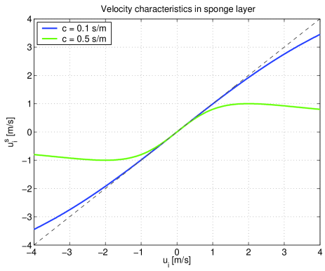
Figure 13: Illustration of the sponge layer characteristics used at open-boundary points to stabilize the vertical-mean velocity when using the sponge layer in combination with ’reduced’ boundary conditions. The green and blue line correspond to sponge-layer curves for $c\neq 0$. The black dashed line denotes the sponge-layer curve for $c=0$.

To stabilize the vertical-mean horizontal velocity components $(u,v)$ at open-boundary grid points, each velocity component is modified according to the following equation:

$$u^{s}_{i}=\frac{\textstyle u_{i}}{\textstyle 1+[c~{}u_{i}]^{2}}$$ (11)

$u_{i}$ denotes the eastward or the northward component, $c$ denotes the sponge-layer parameter, with $c=0$ switching-off the sponge layer. And $u^{s}_{i}$ denotes the velocity value being further used at the open boundary.

In Fig. 13 two sponge-layer curves are depicted for two different sponge-parameter values. It is evident from this figure that the modification of the vertical-mean velocity along the open boundary is very small for small velocity values. In this case, the velocity is not affected by the sponge-layer. Depending on the value of the $c$-parameter, the sponge layer is only effective for larger velocity values which e.g. might be encountered in case of instabilities.

This sponge-layer characteristic after Eq. (11) is symmetric around zero, which might be a disadvantage in case of valid currents at open boundaries which enter or leave the model domain. In this case, the mean velocity of the open-boundary currents might be decreased too much by the sponge-layer. In order to solve this issue, one could use a slightly modified version of Eq. (11). Suppose the model should meet a background current velocity at the open boundary denoted by $u^{b}_{i}$, then the following equation dampens differences to this background velocity wanted:

$$u^{s}_{i}=\frac{\textstyle u_{i}}{\textstyle 1+[c~{}(u_{i}-u^{b}_{i})]^{2}}$$ (12)

Again, within this study, the sponge-layer after Eq. (11) is used.

References

- Barth et al. (2000) Barth, J.A., Pierce, S.D., Smith, R.L., 2000. A separating coastal upwelling jet at Cape Blanco, Oregon and its connection to the California Current System. Deep Sea Research Part II: Topical Studies in Oceanography 47, 783 – 810.
- Bleck (2002) Bleck, R., 2002. An oceanic general circulation model framed in hybrid isopycnic - Cartesian coordinates. Ocean Modelling 37, 55 – 88.
- Centurioni et al. (2008) Centurioni, L.R., Ohlmann, J.C., Niiler, P.P., 2008. Permanent meanders in the california current system. Journal of Physical Oceanography 38, 1690–1710.
- Chassignet et al. (2006) Chassignet, E.P., Hurlburt, H.E., Smedstad, O.M., Halliwell, G.R., Wallcraft, A.J., Metzger, E.J., Blanton, B.O., Lozano, C., Rao, D.B., Hogan, P.J., Srinivasan, A., 2006. Generalized vertical coordinates for eddy-resolving global and coastal ocean forecasts. Oceanography 19.
- Chavez et al. (1994) Chavez, F.P., Herlien, R.A., Thurmond, G.D., 1994. Oasis - acquisition system for moorings/drifters: Developed for interdisciplinary science, with multiple adaptable interfaces; tested on atlas moorings in monterey bay, california. Sea technology 35, 51–59.
- Chavez et al. (2017) Chavez, F.P., Michisaki, R.P., Blum, M., Chavez, G.M., Friederich, J., Jones, B., Herlien, R., Kieft, B., Hobson, B., Ren, A.S., Ryan, J., Sevadjian, J.C., Wahl, C., Walz, K.R., Yamahara, K., Friederich, G.E., Messié, M., 2017. Climate variability and change: Response of a coastal ocean ecosystem. Oceanography .
- Checkley and Barth (2009) Checkley, D.M., Barth, J.A., 2009. Patterns and processes in the California Current System. Progress in Oceanography 83, 49 – 64.
- Chelton (1984) Chelton, D.B., 1984. Seasonal variability of alongshore geostrophic velocity off central California. Journal of Geophysical Research: Oceans 89, 3473 – 3486.
- Chen et al. (2007) Chen, C., Huang, H., Beardsley, R.C., Liu, H., Xu, Q., Cowles, G., 2007. A finite-volume numerical approach for coastal ocean circulation studies: comparisons with finite difference models. Journal of Geophysical Research 112, C03018.
- Chen et al. (2003) Chen, C., Liu, H., Beardsley, R.C., 2003. An unstructured, finite-volume, three-dimensional, primitive equation ocean model: application to coastal ocean and estuaries. Journal of Atmospheric and Oceanic Technology. 20, 159–186.
- Chenillat et al. (2013) Chenillat, F., Rivière, P., Capet, X., Franks, P.J.S., Blanke, B., 2013. California Coastal Upwelling Onset Variability: Cross-Shore and Bottom-Up Propagation in the Planktonic Ecosystem. PLOS ONE 8, 1–15. URL: https://doi.org/10.1371/journal.pone.0062281, doi:10.1371/journal.pone.0062281.
- Collins et al. (2000) Collins, C., Garfield, N., Rago, T., Rischmiller, F., Carter, E., 2000. Mean structure of the inshore countercurrent and California undercurrent off Point Sur, California. Deep Sea Research Part II: Topical Studies in Oceanography 47, 765 – 782.
- Collins et al. (1996) Collins, C., Paquette, R., Ramp, S., 1996. Annual variability of currents at 350 m above the continental slope of Point Sur, California. CalCOFI Reports 37 , 251 – 257.
- Collins et al. (2003) Collins, C., Pennington, J., Castro, C., Rago, T., Chavez, F., 2003. The California Current system off Monterey, California: physical and biological coupling. Deep Sea Research Part II: Topical Studies in Oceanography 50, 2389 – 2404.
- Davis (1985) Davis, R., 1985. Drifter Observations of Coastal Surface Currents During CODE: The Method and Descriptive View. Journal of Geophysical Research 90, 4741–4755. doi:10.1029/JC090iC03p04741.
- Drake et al. (2011) Drake, P.T., Edwards, C.A., Barth, J.A., 2011. Dispersion and connectivity estimates along the U.S. west coast from a realistic numerical model . Journal of Marine Research 69, 1 – 37.
- ECMWF/ERA5 (2017) ECMWF/ERA5, 2017. Copernicus Climate Change Service (C3S). ERA5: Fifth generation of ECMWF atmospheric reanalyses of the global climate. Copernicus Climate Change Service Climate Data Store (CDS). https://cds.climate.copernicus.eu .
- Egbert and Erofeeva (2002) Egbert, G.D., Erofeeva, S.Y., 2002. Efficient inverse modeling of barotropic ocean tides. Journal of Atmospheric and Oceanic Technology 19, 183 – 204.
- Fennel et al. (2006) Fennel, K., Wilkin, J., Levin, J., Moisan, J., O’Reilly, J., Haidvogel, D., 2006. Nitrogen cycling in the middle atlantic bight: Results from a three-dimensional model and implications for the north atlantic nitrogen budget. Global Biogeochemical Cycles 20. GB3007.
- Fiechter et al. (2009) Fiechter, J., Moore, A.M., Edwards, C.A., Bruland, K.W., Lorenzo, E.D., Lewis, C.V., Powell, T.M., Curchitser, E.N., Hedstrom, K., 2009. Modeling iron limitation of primary production in the coastal Gulf of Alaska. Deep Sea Research Part II: Topical Studies in Oceanography 56, 2503 – 2519.
- Fiechter et al. (2020) Fiechter, J., Santora, J.A., Chavez, F., Northcott, D., Messié, M., 2020. Krill hotspot formation and phenology in the california current ecosystem. Geophysical Research Letters 47, e2020GL088039. doi:10.1029/2020GL088039.
- Gangopadhyay et al. (2011) Gangopadhyay, A., Lermusiaux, P.F., Rosenfeld, L., Robinson, A.R., Calado, L., Kim, H.S., Leslie, W.G., Haley, P.J., 2011. The California Current System: A multiscale overview and the development of a feature-oriented regional modeling system (FORMS). Dynamics of Atmospheres and Oceans 52, 131 – 169.
- Gruber et al. (2006) Gruber, N., Frenzel, H., Doney, S.C., Marchesiello, P., Williams, J.C.M., Moisan, J.R., Oram, J.J., Plattner, G.K., Stolzenbach, K.D., 2006. Eddy-resolving simulation of plankton ecosystem dynamics in the California Current System. Deep-Sea Research I 53, 1483 – 1516.
- Haidvogel et al. (2000) Haidvogel, D.B., Arango, H.G., Hedstrom, K., Beckmann, A., Malanotte-Rizzoli, P., Shchepetkin, A.F., 2000. Model evaluation experiments in the North Atlantic Basin: Simulations in nonlinear terrain-following coordinates. Dyn. Atmos. Oceans , 239 – 281.
- Hayward and Mantyla (1990) Hayward, T.L., Mantyla, A.W., 1990. Physical, chemical and biological structure of a coastal eddy near Cape Mendocino. Journal of Marine Research 48, 825–850. doi:10.1357/002224090784988683.
- Hickey (1979) Hickey, B.M., 1979. The California current system - hypotheses and facts. Progress in Oceanography 8, 191 – 279.
- Hickey (1998) Hickey, B.M., 1998. Western North America, tip of Baja California to Vancouver Island. The Sea, Wiley, New York 11, 345 – 394.
- Huyer et al. (1998) Huyer, A., Barth, J., Kosro, P., Shearman, R., Smith, R., 1998. Upper-ocean water mass characteristics of the California current, Summer 1993. Deep Sea Research Part II: Topical Studies in Oceanography 45, 1411 – 1442.
- Jacox et al. (2014) Jacox, M.G., Moore, A.M., Edwards, C.A., , Fiechter, J., 2014. Spatially resolved upwelling in the California Current System and its connections to climate variability. Geophysical Research Letters , 10.1002/2014GL059589.
- Kalnay et al. (1996) Kalnay, E., Kanamitsu, M., Kistler, R., Collins, W., Deaven, D., Gandin, L., Iredell, M., Saha, S., White, G., Woollen, J., Zhu, Y., Chelliah, M., Ebisuzaki, W., Higgins, W., Janowiak, J., Mo, K.C., Ropelewski, C., Wang, J., Leetmaa, A., Reynolds, R., Jenne, R., Joseph, D., 1996. The NCEP/NCAR 40-Year Reanalysis Project. Bulletin of the American Meteorological Society 77, 437 – 472.
- Kämpf and Chapman (2016) Kämpf, J., Chapman, P., 2016. Upwelling Systems of the World. Springer International Publishing.
- Kirchner et al. (2020) Kirchner, J.S., Lettmann, K.A., Schnetger, B., Wolff, J.O., Brumsack, H.J., 2020. Carbon capture via accelerated weathering of limestone: Modeling local impacts on the carbonate chemistry of the southern North Sea. International Journal of Greenhouse Gas Control 92, 102855.
- Kurian et al. (2011) Kurian, J., Colas, F., Capet, X., McWilliams, J.C., Chelton, D.B., 2011. Eddy properties in the California Current System. Journal of Geophysical Research: Oceans 116.
- Levitus (1982) Levitus, S., 1982. CLIMATOLOGICAL ATLAS OF THE WORLD OCEAN, NOAA Professional Paper 13. U.S. Government Printing Office, Washington D.C. , 173pp.
- Lynn and Simpson (1987) Lynn, R.J., Simpson, J.J., 1987. The California Current system: The seasonal variability of its physical characteristics. Journal of Geophysical Research: Oceans 92, 12947–12966.
- Marchesiello et al. (2003) Marchesiello, P., McWilliams, J.C., Shchepetkin, A., 2003. Equilibrium structure and dynamics of the california current system. Journal of Physical Oceanography 33, 753–783.
- Messié and Chavez (2017) Messié, M., Chavez, F.P., 2017. Nutrient supply, surface currents, and plankton dynamics predict zooplankton hotspots in coastal upwelling systems. Geophysical Research Letters 44, 8979–8986. doi:10.1002/2017GL074322.
- Mooers and Robinson (1984) Mooers, C.N.K., Robinson, A.R., 1984. Turbulent Jets and Eddies in the California Current and Inferred Cross-Shore Transports. Science 223, 51 – 53.
- Nagai et al. (2015) Nagai, T., Gruber, N., Frenzel, H., Lachkar, Z., McWilliams, J.C., Plattner, G.K., 2015. Dominant role of eddies and filaments in the offshore transport of carbon and nutrients in the california current system. Journal of Geophysical Research: Oceans 120, 5318–5341.
- Newberger et al. (2003) Newberger, P.A., Allen, J.S., Spitz, Y.H., 2003. Analysis and comparison of three ecosystem models. Journal of Geophysical Research 108.
- Pawlowicz et al. (2002) Pawlowicz, R., Beardsley, B., Lentz, S., 2002. Classical tidal harmonic analysis including error estimates in MATLAB using T-TIDE. Computers and Geosciences 28, 929 – 937.
- Pierce et al. (1996) Pierce, S., Smith, R., Kosro, P., 1996. Observations of the poleward undercurrent along the eastern boundary of the mid-latitude Pacific. EOS, Transactions of the American Geophysical Union 77, F345 (abstract).
- Pierce et al. (2000) Pierce, S., Smith, R., Kosro, P., Barth, J., Wilson, C., 2000. Continuity of the poleward undercurrent along the eastern boundary of the mid-latitude north Pacific. Deep Sea Research Part II: Topical Studies in Oceanography 47, 811 – 829.
- Powell et al. (2006) Powell, T.M., Lewis, C.V.W., Curchitser, E.N., Haidvogel, D.B., Hermann, A.J., Dobbins, E.L., 2006. Results from a three-dimensional, nested biological-physical model of the California Current System and comparisons with statistics from satellite imagery. Journal of Geophysical Research 111, C07018.
- Qi et al. (2009) Qi, J., Chen, C., Beardsley, R.C., Perrie, W., Cowles, G.W., Lai, Z., 2009. An unstructured-grid finite-volume surface wave model (fvcom-swave): Implementation, validations and applications. Ocean Modelling 28, 153–166.
- Reid Jr. and Schwartzlose (1962) Reid Jr., J.L., Schwartzlose, R.A., 1962. Direct measurements of the Davidson Current off central California. Journal of Geophysical Research (1896-1977) 67, 2491 – 2497.
- Sakamoto et al. (2017) Sakamoto, C.M., Johnson, K.S., Coletti, L.J., Maurer, T.L., Massion, G., Pennington, J.T., Plant, J.N., Jannasch, H.W., Chavez, F.P., 2017. Hourly In Situ Nitrate on a Coastal Mooring: A 15-Year Record and Insights into New Production. Oceanography URL: https://doi.org/10.5670/oceanog.2017.428.
- Song et al. (2011) Song, H., Miller, A.J., Cornuelle, B.D., Lorenzo, E.D., 2011. Changes in upwelling and its water sources in the california current system driven by different wind forcing. Dynamics of Atmospheres and Oceans 52, 170–191.
- Spitz et al. (2003) Spitz, Y.H., Newberger, P.A., Allen, J.S., 2003. Ecosystem response to upwelling off the oregon coast: Behavior of three nitrogen-based models. Journal of Geophysical Research: Oceans 108.
- Strub and James (2000) Strub, P., James, C., 2000. Altimeter-derived variability of surface velocities in the California Current System: 2. Seasonal circulation and eddy statistics. Deep Sea Research Part II: Topical Studies in Oceanography 47, 831 – 870.
- Sverdrup et al. (1942) Sverdrup, H., Johnson, M., Fleming, R., 1942. The Oceans: Their Physics, Chemistry and General Biology. Prentice-Hall, Upper Saddle River, New Jersey .
- Umlauf and Burchard (2003) Umlauf, L., Burchard, H., 2003. A generic length-scale equation for geophysical turbulence models. J. Mar. Res. 61, 235 – 265.
- Warner et al. (2005) Warner, J.C., Sherwood, C.R., Arango, H.G., Signell, R.P., 2005. Performance of four turbulence closure models implemented using a generic length scale method. Ocean Modelling 8, 81 – 113.
- Weber and Moore (2013) Weber, E.D., Moore, T.J., 2013. CORRECTED CONVERSION ALGORITHMS FOR THE CALCOFI STATION GRID AND THEIR IMPLEMENTATION IN SEVERAL COMPUTER LANGUAGES. CalCOFI Rep. 54.
- Wilkin et al. (2005) Wilkin, J.L., Arango, H.G., Haidvogel, D.B., Lichtenwalner, C.S., Durski, S.M., Hedstrom, K.S., 2005. A regional Ocean Modeling System for the Long-term Ecosystem Observatory. J. Geophys. Res. 110, C06S91.