Type II critical collapse on a single fixed grid:
a gauge-driven ingoing boundary method

Abstract

We develop a numerical method suitable for gravitational collapse based on Cauchy evolution with an ingoing characteristic boundary. Unlike similar methods proposed recently (Ripley; Bieri, Garfinkle & Yau 2019/20), the numerical grid remains fixed during the evolution and no points need to be removed or added. Increasing coordinate refinement of the central region as the field collapses is achieved solely through the choice of spatial gauge and particularly its boundary condition. We apply this method to study critical collapse of a massless scalar field in spherical symmetry using maximal slicing and isotropic coordinates. Known results on mass scaling, discrete self-similarity and universality of the critical solution (Choptuik 1993) are reproduced using this considerably simpler numerical method.

1 Introduction

Critical phenomena in gravitational collapse are one of the most remarkable discoveries made through numerical methods applied to Einstein’s field equations of general relativity. Since Choptuik’s groundbreaking study of a massless scalar field coupled to the Einstein equations in spherical symmetry Choptuik1993 , similar phenomena have been discovered for a variety of matter models and even in vacuum, see Gundlach2007 for a review article. Briefly, the idea is to choose a smooth one-parameter family of initial data such that in the future Cauchy development of such data, a black hole forms for large parameter values and the field disperses to flat spacetime for small parameter values. We are interested in the threshold between these two final states and the associated critical solution. In what has been termed Type II critical collapse, the black hole mass becomes infinitesimally small as the threshold, obeying a universal scaling law, and the critical solution is discretely self-similar and universal, i.e. independent of the particular one-parameter family of initial data chosen. (There is also Type I critical collapse in certain models, where the black hole mass is finite at the threshold and the critical solution is stationary or time-periodic.)

It is this discrete self-similarity of near-critical evolutions that makes the problem so hard numerically: the solution repeats itself on smaller and smaller spatial scales, in shorter and shorter time intervals. Choptuik Choptuik1993 implemented an adaptive mesh refinement algorithm Berger1984 in order to be able to resolve the increasingly smaller length scales of the solution.

Alternate methods to tackle the same problems have subsequently been developed, e.g. formulations in double null coordinates with Hamade1996 and without Garfinkle1995 adaptive mesh refinement, although in the latter case grid points had to be added during the evolution in order to maintain accuracy.

Recently Bieri, Garfinkle and Yau Bieri2020 proposed a general method for Cauchy evolution in numerical relativity whereby the boundary of the finite spatial computational domain is expanded along a spacelike direction at each time step. Additional initial data must be specified on this surface. The advantage is that with such a setup, no outer boundary conditions need to be imposed because all the constant-time slices lie within the domain of dependence of the initial slice and the additional “tilted” spacelike surface. This proposal thus avoids the long-standing problem of imposing boundary conditions along a finite timelike surface in general relativity Sarbach2007 . Other alternatives to this problem include Cauchy-characteristic matching Winicour2012 , evolution on hyperboloidal slices compactified towards future null infinity Zenginoglu2008 ; Moncrief2009 ; Rinne2010 and the regular conformal field equations Friedrich1983 ; Frauendiener2004 .

Related to Bieri et al.’s scheme is the “excision method” proposed by Ripley Ripley2019 , whereby the computational domain is excised along a surface that is spacelike or tangent to an ingoing characteristic of the boundary on the initial slice. Again, no boundary conditions need to be impose at the outer boundary because in this case all characteristics leave the computational domain. This method appears to be well suited to gravitational collapse problems. A disadvantage is that grid points are lost during the evolution due to the excision procedure so that one will have to add grid points in the interior in order to maintain accuracy.

The method developed in the present paper is similar to Ripley’s in that the outer boundary of the spatial computational domain is an ingoing characteristic. However, no grid points are excised; instead merely the spatial coordinates are changed as time proceeds.

In the Arnowitt-Deser-Misner (ADM) formulation of general relativity Arnowitt1962 , the time vector field $\partial/\partial t$ is decomposed as

$$\left(\textstyle\frac{\partial}{\partial t}\right)^{a}=\alpha n^{a}+\beta^{a},$$ (1)

where $n_{a}=-\alpha\nabla_{a}t$ is the unit future-directed timelike normal, $\alpha$ is the lapse function and $\beta^{a}$ the shift vector (which is spatial, $n_{a}\beta^{a}=0$). This means that a point with spatial coordinates $x^{i}$ on the spatial slice at time $t$ correponds to the point with spatial coordinates $x^{i}-\beta^{i}\mathrm{d}t$ on the slice at time $t+\mathrm{d}t$ if we drag it along the timelike normal.

Consider now a shift vector field of the form

$$\beta^{i}=cx^{i}$$ (2)

where $c$ is a constant w.r.t. the spatial coordinates $x^{i}$. Hence identified points on the spatial slices will change coordinates according to

$$x^{i}\rightarrow(1-c\,\mathrm{d}t)x^{i}$$ (3)

as time increases from $t$ to $t+\mathrm{d}t$, so if we choose $c<0$ then the coordinates “zoom in” isotropically towards the origin. The significance of (2) is that it is a homogeneous solution to the spatial isotropic gauge condition in spherical symmetry, Eq. (11) below, where $\beta^{r}=r\beta$ so (2) corresponds to $\beta=c=\mathrm{const}$. The value of the constant $c$ will be fixed by the boundary condition on the shift in the isotropic gauge condition. For a suitable value of this (in general time-dependent) constant, the outer boundary can be made an ingoing characteristic (or spacelike) so that no boundary conditions on the evolved fields are needed.

We supplement the isotropic spatial gauge condition with a maximal slicing condition. The advantage of such a slicing as compared with the polar slicing used by Choptuik Choptuik1993 is that the coordinates remain regular at the apparent horizon when it forms, which allows for a more accurate determination of its location and mass.

This article is organised as follows. In Sect. 2 we set up our model problem of a massless scalar field in spherical symmetry, and we state the gauge conditions and their boundary conditions appropriate for our ingoing boundary method. In Sect. 3 we provide details on the numerical methods we use to solve the field equations. The numerical results are contained in Sect. 4. We set up two families of initial data, describe our method to tune to the critical parameter and to choose an appropriate outer boundary radius, and we present results on the mass scaling, discrete self-similarity and universality of the critical solution. In Sect. 5 we summarise, discuss potential challenges of the method and future applications.

2 Formulation of the model

2.1 Choice of gauge and variables

In spherical symmetry and isotropic coordinates, the spacetime metric takes the form

$$ds^{2}=-(\alpha^{2}-\psi^{4}r^{2}\beta^{2})\mathrm{d}t^{2}+2r\beta\psi^{4}\mathrm{d}t\,\mathrm{d}r+\psi^{4}\left[\mathrm{d}r^{2}+r^{2}(\mathrm{d}\theta^{2}+\sin^{2}\theta\,\mathrm{d}\varphi^{2})\right].$$ (4)

We impose maximal slicing and hence the extrinsic curvature has only one independent component in spherical symmetry:

$$K^{i}{}_{j}=\mathrm{diag}(K^{r}{}_{r},-\textstyle\frac{1}{2}K^{r}{}_{r},-\textstyle\frac{1}{2}K^{r}{}_{r}).$$ (5)

For reasons discussed shortly, we define a rescaled quantity

$${\hat{K}^{r}{}_{r}}:=r^{-2}\psi^{6}K^{r}{}_{r}.$$ (6)

The massless scalar field $\Phi$ itself does not enter the equations but only its first derivatives

$${\hat{\xi}}:=r^{-1}\psi^{2}\Phi^{\prime},\qquad{\hat{\Pi}}:=\psi^{4}\alpha^{-1}(\dot{\Phi}-r\beta\Phi^{\prime}),$$ (7)

where here and in the following a dash denotes a partial derivative w.r.t. $r$ and a dot w.r.t. $t$.

The fundamental variables $\alpha,\beta,\psi,{\hat{K}^{r}{}_{r}},{\hat{\xi}}$ and ${\hat{\Pi}}$ depend on $t$ and $r$ only, and the powers of $r$ in their definitions have been chosen so that they are all even functions of $r$ with finite nonzero limits at the origin $r=0$.

2.2 Field equations

The relevant components of the Einstein equations $R_{ab}=\kappa\nabla_{a}\nabla_{b}\Phi$, where $R_{ab}$ is the spacetime Ricci tensor and $\kappa=8\pi$ in geometric units, are the momentum constraint

$$r{\hat{K}^{r}{}_{r}}^{\prime}+5{\hat{K}^{r}{}_{r}}+\kappa\hat{\pi}\hat{\xi}=0$$ (8)

and the Hamiltonian constraint

$$\psi^{\prime\prime}+2r^{-1}\psi^{\prime}+\textstyle\frac{3}{16}\psi^{-7}(r^{2}{\hat{K}^{r}{}_{r}})^{2}+\textstyle\frac{1}{8}\kappa\psi^{-3}({\hat{\Pi}}^{2}+r^{2}{\hat{\xi}}^{2})=0.$$ (9)

When linearising (9) about a given background solution $\overline{\psi}$, the coefficient of the undifferentiated term proportional to $\psi$ is manifestly negative because of the negative powers of $\psi$ in (9). If this was not the case then non-unique oscillatory solutions might exist; see Walsh2007 ; Rinne2008 for further discussion of this issue. This is the reason for the choice of the powers of $\psi$ in (6) and (7).

The maximal slicing condition implies the following equation for the lapse,

$$\alpha^{\prime\prime}+2\alpha^{\prime}(r^{-1}+\psi^{-1}\psi^{\prime})-\alpha\left[\kappa\psi^{-4}{\hat{\Pi}}^{2}+\textstyle\frac{3}{2}\psi^{-8}(r^{2}{\hat{K}^{r}{}_{r}})^{2}\right]=0,$$ (10)

and preservation of the isotropic form of the metric (4) yields

$$\beta^{\prime}-\textstyle\frac{3}{2}r\alpha\psi^{-6}{\hat{K}^{r}{}_{r}}=0.$$ (11)

The equation of motion for the scalar field $\nabla^{a}\nabla_{a}\Phi=0$ reduces to the pair of first-order equations

$$\dot{\hat{\xi}} = r\beta{\hat{\xi}}^{\prime}+(3\beta+2\alpha\psi^{-6}r^{2}{\hat{K}^{r}{}_{r}}){\hat{\xi}}+\alpha\psi^{-2}r^{-1}{\hat{\Pi}}^{\prime}$$ (12)

$$+\psi^{-3}r^{-1}(\psi\alpha^{\prime}-4\alpha\psi^{\prime}){\hat{\Pi}},$$

$$\dot{\hat{\Pi}} = r\beta{\hat{\Pi}}^{\prime}+(2\beta+\alpha\psi^{-6}r^{2}{\hat{K}^{r}{}_{r}}){\hat{\Pi}}+\alpha\psi^{-2}r{\hat{\xi}}^{\prime}+\psi^{-2}(r\alpha^{\prime}+3\alpha){\hat{\xi}}.$$ (13)

There are redundant evolution equations for $\psi$ and ${\hat{K}^{r}{}_{r}}$ that can be used to monitor the accuracy of the code; the first will also be needed to specify boundary conditions:

$$\dot{\psi} = r\beta\psi^{\prime}+\textstyle\frac{1}{2}\beta\psi+\textstyle\frac{1}{4}r^{2}\alpha\psi^{-5}{\hat{K}^{r}{}_{r}},$$ (14)

$$\dot{\hat{K}^{r}{}_{r}} = r\beta{\hat{K}^{r}{}_{r}}^{\prime}+5\beta{\hat{K}^{r}{}_{r}}+\textstyle\frac{3}{2}\alpha r^{2}\psi^{-6}{\hat{K}^{r}{}_{r}}^{2}-\textstyle\frac{2}{3}\psi^{2}r^{-1}(r^{-1}\alpha^{\prime})^{\prime}$$ (15)

$$-\textstyle\frac{4}{3}\alpha\psi r^{-1}(r^{-1}\psi^{\prime})^{\prime}+4r^{-2}\psi^{\prime}(\alpha\psi^{\prime}+\textstyle\frac{2}{3}\psi\alpha^{\prime})-\textstyle\frac{2}{3}\kappa\alpha\psi^{-2}{\hat{\xi}}^{2}.$$

2.3 Boundary conditions

A crucial feature of our method is the choice of gauge boundary conditions. We want the outer boundary to be ingoing null or spacelike, which corresponds to setting

$$\beta\doteq-\nu\,r^{-1}\psi^{-2}\alpha$$ (16)

with $\nu\geqslant 1$, where $\doteq$ means equality at the outer boundary $r=r_{\max}$. For the results presented in Sect. 4 we will always choose $\nu=1$ corresponding to the boundary being null, although we will briefly discuss making $\nu$ a time-dependent function in Sect. 5.

Since there are no ingoing characteristics at the outer boundary with this choice, the evolution equations (12) and (13) for the scalar field do not require any boundary conditions. We specify Dirichlet boundary conditions on $\psi$ for the Hamiltonian constraint (9) by evolving (14) at the outer boundary. The momentum constraint (8) does not require a boundary condition as this is already fixed by demanding the solution to be regular at the origin.

What remains to be specified is an outer boundary condition on the lapse $\alpha$ for the maximal slicing condition (10). Freezing the lapse to its flat value $\alpha=1$ is not a good idea since this will lead to unacceptably large slice stretching as the physical size of the grid shrinks and the lapse collapses in the centre as the singularity is approached. Instead we simply advect the lapse along the shift at the outer boundary, as in the first terms of all the evolution equations:

$$\dot{\alpha}\doteq r\beta\alpha^{\prime}.$$ (17)

Another way of phrasing this is to extrapolate (in time) the value of the lapse at the outer boundary $r=r_{\max}$ on the slice at time $t+\mathrm{d}t$ from its value at the identified radius on the slice at time $t$, which according to (3) is at $(r+r\beta\mathrm{d}t)_{r=r_{\max}}<r_{\max}$ (note $\beta<0$ at $r=r_{\max}$).

3 Numerical methods

3.1 Evolution scheme

Given data at time $t$, we first evolve the scalar field variables ${\hat{\xi}}$ and ${\hat{\Pi}}$ to the next timestep $t+\Delta t$ using (12) and (13). At the advanced time the radial ordinary differential equations (ODEs) (8)–(11) are solved in this order for ${\hat{K}^{r}{}_{r}},\psi,\alpha$ and $\beta$ (notice they form a hierarchy). Dirichlet boundary values for $\psi$ and $\alpha$ are supplied by evolving (14) and (17) at the outer boundary along with the other evolution equations, and the boundary condition for $\beta$ is (16).

3.2 Discretisation

We use a fixed non-uniform radial grid at points $r_{i}=f(x_{i})$, where

$$f:[0,1]\to[0,r_{\max}],\quad f(x)=r_{\mathrm{eff}}x+(r_{\max}-r_{\mathrm{eff}})x^{3}$$ (18)

is a cubic map from numerical to physical coordinates. Here $r_{\mathrm{eff}}\leqslant r_{\max}$ can be thought of as an “effective” radius the grid would have if the same resolution as close to the origin was used all the way to the outer boundary. We typically choose $r_{\mathrm{eff}}\approx\textstyle\frac{1}{2}r_{\max}$. It should be noted that a non-uniform grid is not essential for our method to work, it just saves computational resources since the distribution of grid points is better adapted to the features of the solution, which has its largest gradients close to the origin. We could just as well take $r_{\mathrm{eff}}=r_{\max}$ corresponding to a uniform grid. With respect to the numerical coordinate $x$, the grid is equidistant and staggered at the origin:

$$x_{i}=(i+\textstyle\frac{1}{2})h,\quad i=0,1,\ldots,N,\quad h=(N+\textstyle\frac{1}{2})^{-1}.$$

We use $N=500$ grid points for the simulations presented in Sect. 4. The grid remains unchanged during the evolution.

We use centred fourth-order finite differences to discretise the equations in $r$. Near the origin the finite-difference stencils are modified according to the known (even) $r$-parity of all the evolved variables. Near the outer boundary (fourth-order) backward finite differences are used.

3.3 ODE solvers

Following the method of lines, the evolution equations are integrated forward in time using a standard fourth-order Runge-Kutta method. Sixth-order Kreiss-Oliger dissipation Kreiss1973 is added to the right-hand sides of the evolution equations in order to maintain numerical stability (a small coefficient $\approx 0.1$ is found to be sufficient).

The radial ODEs are solved using a direct band-diagonal solver at each substep of the Runge-Kutta method.

Since the size of the metric functions $\alpha,\beta$ and $\psi$ changes drastically during the evolution, it is important to adapt the size of the time step $\Delta t$ in order not to violate the Courant-Friedrichs-Lewy (CFL) condition for numerical stability. At each time step, we compute the characteristic speeds of the scalar wave equation

$$v_{\pm}(r)=-r\beta\pm\psi^{-2}\alpha$$ (19)

and set the time step size according to

$$\Delta t=\lambda\min_{i=1,\ldots,N}\frac{r_{i}-r_{i-1}}{\max(|v_{+}(r_{i})|,|v_{-}(r_{i})|)}.$$ (20)

The CFL condition states $0<\lambda<1$, and we typically choose $\lambda=\textstyle\frac{1}{2}$.

3.4 Termination criteria

We terminate a simulation when either a black hole forms (i.e. the evolution is supercritical) or the field disperses to flat spacetime (i.e. the evolution is subcritical).

Formation of a black hole is detected by looking for an apparent horizon (outermost marginally outer trapped surface). This is an $r=\mathrm{const}$ surface whose outgoing null expansion vanishes,

$$\theta_{+}=2(\ln R)_{,a}\ell^{a}=0,$$ (21)

where

$$R=r\psi^{2}$$ (22)

is the areal radius and $\ell^{a}$ is an outward-pointing radial null vector. In our variables (21) is equivalent to

$$r\psi^{\prime}+\textstyle\frac{1}{2}\psi+\textstyle\frac{1}{4}r^{3}\psi^{-3}{\hat{K}^{r}{}_{r}}=0.$$ (23)

The radius $r_{\mathrm{AH}}$ of the apparent horizon is the largest zero of this equation, and the associated mass is

$$M=\textstyle\frac{1}{2}R|_{r=r_{\mathrm{AH}}}.$$ (24)

It is this mass computed from the apparent horizon that will enter the scaling law in Sect. 4.3. Assuming cosmic censorship holds, formation of an apparent horizon implies the existence of an event horizon containing the apparent horizon in its interior.

We consider an evolution to be subcritical if the maximum (w.r.t. $r$) of the scalar curvature

$$\mathcal{R}=\kappa\psi^{-8}\left[(r{\hat{\xi}})^{2}-{\hat{\Pi}}^{2}\right]$$ (25)

drops below some fraction (typically $5\%$) of its maximum value attained during the evolution.

4 Numerical results

4.1 Initial data and bisection

We consider two very different families of initial data for the scalar field:
(i) data that would be exactly ingoing in a flat metric ($\psi=\alpha=1,\,\beta=0$),

$$\Phi=A\,\exp\left[-\frac{1}{2}\left(\frac{r-r_{0}}{\sigma}\right)^{2}\right],\quad{\hat{\xi}}=r^{-1}\Phi^{\prime},\quad{\hat{\Pi}}=r^{-1}(r\Phi)^{\prime},$$ (26)

and (ii) data that are centred at the origin and initially at rest,

$$\Phi=A\,\exp\left[-\frac{1}{2}\left(\frac{r}{\sigma}\right)^{2}\right],\quad{\hat{\xi}}=r^{-1}\Phi^{\prime},\quad{\hat{\Pi}}=0.$$ (27)

We fix the parameters $\sigma=1$ and (for the ingoing family) $r_{0}=10$, and we take the amplitude $A$ as the critical parameter. For large values of $A$ the solution forms a black hole whereas for small values it disperses. We use the bisection method to find an approximation to the critical amplitude $A_{*}$.

4.2 Choosing the outer boundary radius

A typical Penrose diagram of a supercritical evolution close to the critical point is shown in Fig. 1. It becomes obvious from this diagram that the success of our method will depend on a good choice of the radius $r_{\max}$ of the outer boundary on the initial spatial slice.

Figure 1: Penrose diagram of a typical near-critical spacetime. Shown are the initial spatial slice at $t=0$ and a number of subsequent spatial slices and their ingoing null boundaries for two different initial boundary radii $r_{1}$ and $r_{2}$ as discussed in the main text. On the last slice the apparent horizon (AH) forms, which at later times converges to the event horizon (EH) of the black hole. Spacetime is close to the Type II critical solution roughly in the shaded region.

If this is taken to be too large, $r_{\max}=r_{2}$ in Fig. 1, then despite the fact that the outer boundary is an ingoing characteristic, the apparent horizon forms at a very small radius compared to the radius of the outer boundary. We terminate the bisection scheme if the radius of the apparent horizon in the supercritical evolutions gets too small, say $r_{\mathrm{AH}}<0.01\,r_{\max}$, and start over with a smaller value of $r_{\max}$.

If on the other hand the initial boundary radius is chosen too small, $r_{\max}=r_{1}$ in Fig. 1, then the field escapes from the spatial domain before the apparent horizon forms. In a numerical evolution of this type we observe that the bulk of the scalar field moves out of the domain but the scalar curvature (25) remains large, unlike in a subcritical evolution. If this happens, we terminate the bisection scheme and repeat it with a larger value of $r_{\max}$.

Essentially this adds an outer bisection loop (for $r_{\max}$) to the inner one (for $A$). In practice, one does not have to repeat the $A$-bisection all the way from the start because one can use a somewhat smaller $A$-interval of the previous $r_{\max}$-iteration as the initial interval for the $A$-bisection at the improved value of $r_{\max}$.

Using this procedure we determine $r_{\max}^{(i)}=15.421875$ for the ingoing family and $r_{\max}^{(ii)}=5.64$ for the centred family. (For comparison, the near-critical ADM masses are $M_{\mathrm{ADM}}^{(i)}=0.27$ and $M_{\mathrm{ADM}}^{(ii)}=0.41$.) Being able to observe the mass scaling (Sect. 4.3) does not require such a precise choice of $r_{\max}$, while for the echoing behaviour of the critical solution (Sect. 4.4) more accuracy is needed. (About three echos were visible in the simulations reported here.)

To provide some idea of how the physical size of the grid changes during a simulation, we plot in Fig. 2 the areal radius $R_{\max}$ of the outer boundary as a function of the number of time steps $n$ for a near-critical evolution. The exponential decrease of $R_{\max}$ with $n$ is well adapted to the expected discrete self-similarity of the critical solution, which repeats itself on smaller and smaller scales. Also shown in Fig. 2 are the coordinate time $t$ and proper time at the origin

$$T_{0}(t)=\int_{0}^{t}\alpha(\tilde{t},0)\mathrm{d}\tilde{t}$$ (28)

as functions of the number of time steps $n$. The latter approaches the accumulation time $T_{0}^{*}$ of the critical solution.

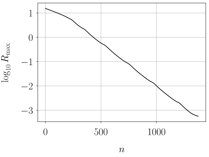
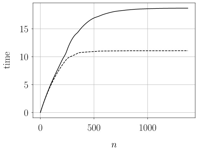
Figure 2: Left: areal radius $R_{\max}$ as a function of the number of time steps $n$. Right: coordinate time $t$ (solid curve) and proper time at the origin $T_{0}$ (dashed curve) as functions of $n$.

4.3 Mass scaling

In Fig. 3 we plot the apparent horizon mass $M$ vs. the distance $A-A_{*}$ to the critical amplitude for a series of supercritical evolutions. In a double-logarithmic plot this forms a straight line with a periodic wiggle:

$$\ln(M)=\gamma\ln(A-A_{*})+\Psi[\ln(A-A_{*})]+\mathrm{const},$$ (29)

as first observed numerically in Choptuik1993 ; Hod1997 and predicted from a perturbative analysis of the critical solution in Hod1997 ; Gundlach1997 . According to this analysis, the period $\varpi$ of the function $\Psi$ is related to the echoing exponent $\Delta$ (cf. Sect. 4.4) via $\Delta=2\varpi\gamma$. The values of the mass scaling exponent $\gamma$ and the echoing exponent $\Delta$ obtained from a fit to our numerical data are shown in Table 1 and are in good agreement with the predicted values. It should be noted that $\Delta$ can be determined more accurately from the echoing behaviour of the near-critical solution (Sect. 4.4).

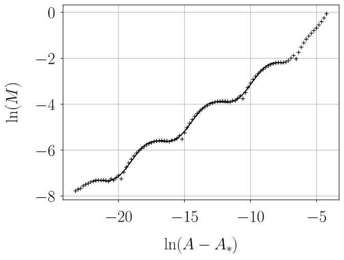
Figure 3: Apparent horizon mass $M$ vs. critical parameter distance $A-A_{*}$ in a double-logarithmic plot for a series of supercritical evolutions of the ingoing family ($+$) and best fit using the function $f(x)=c_{0}+c_{1}x+c_{2}\cos(c_{3}+c_{4}x)$ (solid curve).

	fit ingoing family (i)	fit centred family (ii)	prediction
$\gamma$	$0.3744\pm 0.0017$	$0.3738\pm 0.0027$	$0.374\pm 0.001$
$\Delta$	$3.419\pm 0.033$	$3.442\pm 0.058$	$3.4453\pm 0.0005$

Table 1: Mass scaling exponent $\gamma$ and echoing exponent $\Delta$ fitted from the numerical values of the mass for the two initial data families, and their predictions from a perturbative analysis of the critical solution Gundlach1997 .

4.4 Discrete self-similarity and universality of the critical solution

Variables that are scale invariant display discrete self-similarity in near-critical evolutions. One such scale-invariant variable for the scalar field is

$$X:=r\Phi^{\prime}=r^{2}\psi^{-2}{\hat{\xi}}.$$ (30)

Discrete self-similarity is best described in terms of logarithmic coordinates

$$\tau:=\ln(T_{0}^{*}-T_{0}),\qquad\rho:=\ln R,$$ (31)

where $T_{0}^{*}$ is the accumulation time of the critical solution. The conjecture, first discovered numerically in Choptuik1993 , is that for the critical solution (indicated by the star), any scale-invariant variable such as $X$ (30) obeys

$$X_{*}(\rho-\Delta,\tau-\Delta)=X_{*}(\rho,\tau),$$ (32)

where $\Delta$ is the echoing exponent.

In Fig. 4 we plot $X^{(i)}(\rho,\tau)$ for a near-critical evolution of the ingoing family as a function of $\rho$ at two different times $\tau$, and we overlay $X^{(i)}(\rho-\Delta,\tau-\Delta)$ in the same plots, using $\Delta=3.44$. The accumulation time $T_{0}^{*}$ has been determined by minimising the norm of the difference between both functions at one fixed time $\tau$. The fact that the curves nearly coincide provides strong support of the echoing property (32). We can also see in Fig. 4 that the solution is well resolved numerically both at the original time $\tau$ and at the time of the echo $\tau-\Delta$, when the spatial scale has shrunk by a factor $\mathrm{e}^{\Delta}\approx 31$.

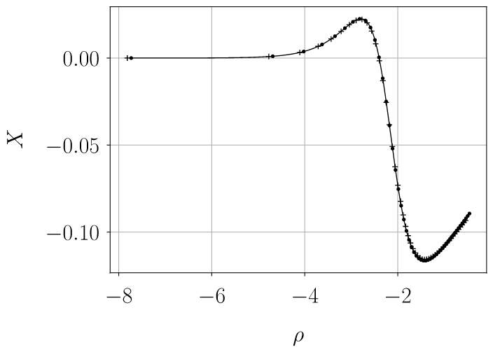
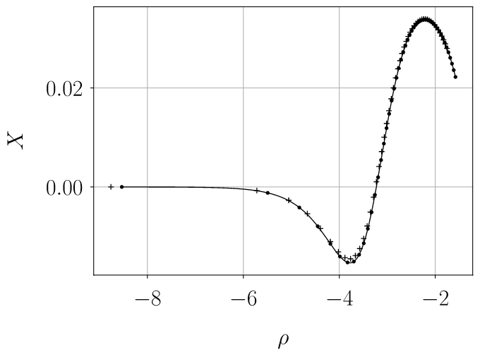
Figure 4: Discrete self-similarity: the scale-invariant variable $X^{(i)}(\tau,\rho)$ for a near-critical evolution of the ingoing family is plotted as a function of $\rho$ at two different times $\tau=-1.8$ (left) and $\tau=-3.1$ (right) as a solid curve with dots at every tenth grid point. In the same plots, we also show $X^{(i)}(\tau-\Delta,\rho-\Delta)$ as a function of $\rho$ with plus symbols ($+$) at every tenth grid point. The echoing exponent is taken to be $\Delta=3.44$.

Finally we investigate if the critical solution is universal, i.e. independent of the particular one-parameter family of initial data. In Fig. 5 we again plot $X^{(i)}(\rho,\tau)$ for a near-critical evolution of the ingoing family as a function of $\rho$ at two different times $\tau$, but this time we overlay $X^{(ii)}(\rho-\delta,\tau-\delta)$ for a near-critical evolution of the centred family, where $\delta$ is an overall family-dependent scale chosen such that the norm of the difference between the two solutions is minimal at one fixed $\tau$. The fact that the curves nearly coincide also at a different time $\tau$ with the same constant offset $\delta$ strongly supports the conjecture that the critical solution is universal, as already argued in Choptuik1993 .

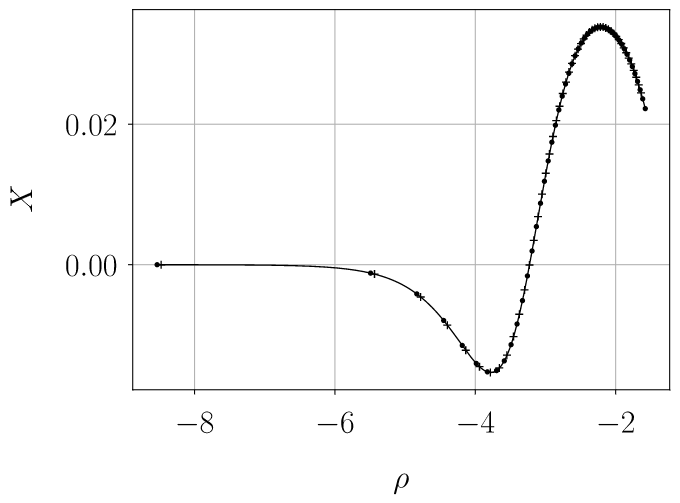
Figure 5: Universality: the scale-invariant variable $X^{(i)}(\tau,\rho)$ for a near-critical evolution of the ingoing family is plotted as a function of $\rho$ at two different times $\tau=-1.8$ (left) and $\tau=-3.1$ (right) as a solid curve with dots at every tenth grid point. In the same plots, we also show $X^{(ii)}(\tau-\delta,\rho-\delta)$ for a near-critical evolution of the centred family with plus symbols ($+$) at every tenth grid point. The same (family-dependent) constant offset $\delta=0.245$ is used in both plots.

5 Discussion

We presented a numerical method for gravitational collapse based on Cauchy evolution with an ingoing null boundary. The method is similar in spirit to the excision method of Ripley Ripley2019 but differs in that no grid points are removed from the computational domain; rather, the grid remains fixed and only the coordinates are adapted along with the evolution. This is achieved by adding a linear term to the shift vector that causes the coordinates to “zoom in” isotropically towards the centre. This linear term is a homogeneous solution to the isotropic spatial gauge condition. Another important ingredient is the treatment of the lapse function. We propose to use an advection equation for the lapse along the shift vector at the outer boundary in order to provide boundary values for the slicing condition (in our case, maximal slicing). This corresponds to interpolating the lapse from the previous time step and minimises the amount of slice stretching as the lapse collapses towards zero in the high curvature region in the centre.

We worked out the method in detail for the model problem of a massless scalar field coupled to the Einstein equations in spherical symmetry. Known results on critical behaviour Choptuik1993 are reproduced: the mass-scaling relation including its fine structure Hod1997 ; Gundlach1997 , the discrete self-similarity (echoing) of the critical solution and its universality among different families of initial data. This demonstrates that the method is well suited to studying critical phenomena in gravitational collapse, while being considerably simpler than more commonly used methods that typically employ adaptive mesh refinement.

A price one has to pay for the simplicity of the method is that the outer boundary radius $r_{\max}$ of the initial data slice needs to be chosen carefully so that a sufficiently large region of spacetime where the evolution is close to the critical solution can be explored. We optimised $r_{\max}$ using an outer bisection loop depending on the outcome of the standard inner bisection along the critical parameter. One might wonder if this makes the method overly computationally expensive. Certainly in spherical symmetry this is not the case as a single evolution takes less than five minutes on a laptop even close to the critical point. Furthermore one does not have to restart the bisection for the critical parameter from the beginning for each $r_{\max}$ iteration; instead, a smaller interval from the previous bisection can be used as an improved initial guess. Whether the method is competitive in axisymmetry or without any spacetime symmetries remains to be seen.

We have tried to alleviate the need for fine-tuning $r_{\max}$ by equipping the algorithm with a control system similar to the one described in Lindblom2007 : make $\nu$ in (16) time dependent and steer it so that a typical feature of the solution such as the minimum of the outgoing expansion (21) remains approximately at a constant coordinate radius. The larger the value of $\nu$, the stronger the magnifying effect. For this to work, $r_{\max}$ must be chosen somewhat larger than its optimal value for a null boundary, and $\nu$ must be taken somewhat larger than $1$ initially, so that the control system has enough room to do its job. While performing reasonably well at early times, we have found such a control system to be ineffective in halting the rapid escape of the scalar field from the domain that often occurs just before an apparent horizon forms if the initial $r_{\max}$ was chosen too small or the control system kept $\nu$ too large for too long a time. One should note that $\nu$ must not get smaller than $1$, otherwise the boundary becomes timelike and boundary conditions for the evolved fields are needed.

Let us finally comment on other gauge conditions and less restrictive spacetime symmetries. In axisymmetry there is the well-known quasi-isotropic (or isothermal) gauge in which the spatial metric takes the form (compare (4))

$${}^{(3)}ds^{2}=\phi^{4}\mathrm{e}^{2\eta/3}(\mathrm{d}r^{2}+r^{2}\mathrm{d}\theta^{2}+\mathrm{e}^{-2\eta}r^{2}\sin^{2}\theta\,\mathrm{d}\varphi^{2}).$$ (33)

This has been used in much numerical work, including the first study of critical behaviour in vacuum axisymmetric gravitational collapse by Abrahams and Evans Abrahams1993 , as well as e.g. Rinne2008 ; Garfinkle2001 ; Choptuik2003 ; Choptuik2003a ). The quasi-isotropic gauge condition admits homogeneous solutions analogous to the isotropic gauge condition in spherical symmetry, and our method can be carried over with very few modifications. Work along these lines is in progress.

It is conceivable that our method can be made to work with other classes of spatial gauge conditions as well. Any elliptic shift condition such as the minimal strain or minimal distortion conditions Smarr1978 requires boundary conditions, and the freedom in choosing the boundary data can be used to make the outer boundary an ingoing null surface. Evolutionary shift conditions such as the hyperbolic Gamma-driver condition employed in some of the first successful binary black hole merger simulations Campanelli2006 require initial conditions, and they could also be modified by adding lower-order terms, which could be used to a similar effect. These are interesting questions for further research.

Finally it should be stressed that this ingoing boundary method or the related method of Ripley Ripley2019 are not limited to studying critical collapse. One can also start with a standard Cauchy evolution with timelike boundary (where of course boundary conditions must be imposed) and switch to the ingoing boundary method at a certain time. Combinations with the outgoing boundary method of Bieri et al.Bieri2020 are also possible.

- (1) M.W. Choptuik: Universality and scaling in gravitational collapse of a massless scalar field. Phys. Rev. Lett. 70, 9 (1993)
- (2) C. Gundlach, J.M. Martín-García: Critical phenomena in gravitational collapse. Living Rev. Relativity 10(5) (2007)
- (3) M.J. Berger, J. Oliger: Adaptive mesh refinement for hyperbolic partial differential equations. J. Comput. Phys. 53, 484 (1984)
- (4) R.S. Hamadé, J.M. Stewart: The spherically symmetric collapse of a massless scalar field. Class. Quantum Grav. 13, 497 (1996)
- (5) D. Garfinkle: Choptuik scaling in null coordinates. Phys. Rev. D 51, 5558 (1995)
- (6) L. Bieri, D. Garfinkle, S.T. Yau: A no-boundary method for numerical relativity. Class. Quantum Grav. 37, 045015 (2020)
- (7) O. Sarbach: Absorbing boundary conditions for Einstein’s field equations. J. Phys.: Conf. Ser. 91, 012005 (2007)
- (8) J. Winicour: Characteristic evolution and matching. Living Rev. Relativity 15(2) (2012)
- (9) A. Zenginoğlu: Hyperbolodial evolution with the Einstein equations. Class. Quantum Grav. 25, 195025 (2008)
- (10) V. Moncrief, O. Rinne: Regularity of the Einstein equations at future null infinity. Class. Quantum Grav. 26, 125010 (2009)
- (11) O. Rinne: An axisymmetric evolution code for the Einstein equations on hyperboloidal slices. Class. Quantum Grav. 27, 035014 (2010)
- (12) H. Friedrich: Cauchy problems for the conformal vacuum field equations in general relativity. Commun. Math. Phys. 91, 445 (1983)
- (13) J. Frauendiener: Conformal infinity. Living Rev. Relativity 7(1) (2004)
- (14) J.L. Ripley: Excision and avoiding the use of boundary conditions in numerical relativity. Class. Quantum Grav. 36, 237001 (2020)
- (15) R. Arnowitt, S. Deser, C.W. Misner: The dynamics of general relativity. In Gravitation: an introduction to current research, ed. by L. Witten (Wiley, New York, 1962), chap. 7
- (16) D.M. Walsh: Non-uniqueness in conformal formulations of the Einstein constraints. Class. Quantum Grav. 24, 1911 (2007)
- (17) O. Rinne: Constrained evolution in axisymmetry and the gravitational collapse of prolate Brill waves. Class. Quantum Grav. 25, 135009 (2008)
- (18) H.O. Kreiss, J. Oliger: Methods for the approximate solution of time dependent problems. Global Atmospheric Research Programme, Publication Series No. 10 (1973)
- (19) S. Hod, T. Piran: Fine structure of Choptuik’s mass-scaling relation. Phys. Rev. D 55, R440 (1997)
- (20) C. Gundlach: Understanding critical collapse of a scalar field. Phys. Rev. D 55, 695 (1997)
- (21) L. Lindblom, K.D. Matthews, O. Rinne, M.A. Scheel: Gauge drivers for the generalized harmonic Einstein equations. Phys. Rev. D 77, 084001 (2008)
- (22) A.M. Abrahams, C.R. Evans: Critical behavior and scaling in vacuum axisymmetric gravitational collapse. Phys. Rev. Lett. 70, 2980 (1993)
- (23) D. Garfinkle, G.C. Duncan: Numerical evolution of Brill waves. Phys. Rev. D 63, 044011 (2001)
- (24) M.W. Choptuik, E.W. Hirschmann, S.L. Liebling, F. Pretorius: An axisymmetric gravitational collapse code. Class. Quantum Grav. 20, 1857 (2003)
- (25) M.W. Choptuik, E.W. Hirschmann, S.L. Liebling, F. Pretorius: Critical collapse of the massless scalar field in axisymmetry. Phys. Rev. D 68, 044007 (2003)
- (26) L. Smarr, J.W. York: Kinematical conditions in the construction of spacetime. Phys. Rev. D 17, 2529 (1978)
- (27) M. Campanelli, C.O. Lousto, P. Marronetti, Y. Zlochower: Accurate evolutions of orbiting black-hole binaries without excision. Phys. Rev. Lett. 96, 111101 (2006)