Generalized Lee Bounds

Abstract

Lee (2009) is a common approach to bound the average causal effect in the presence of selection bias, assuming the treatment effect on selection has the same sign for all subjects. This paper generalizes Lee bounds to allow the sign of this effect to be identified by pretreatment covariates, relaxing the standard (unconditional) monotonicity to its conditional analog. Asymptotic theory for generalized Lee bounds is proposed in low-dimensional smooth and high-dimensional sparse designs. The paper also generalizes Lee bounds to accommodate multiple outcomes. It characterizes the sharp identified set for the causal parameter and proposes uniform Gaussian inference on the support function. The estimated bounds achieve nearly point-identification in JobCorps job training program (Lee (2009)), where unconditional monotonicity is unlikely to hold.

1 Introduction

Randomized controlled trials are often complicated by endogenous sample selection and non-response. This problem occurs when treatment affects the researcher’s ability to observe an outcome (a selection effect) in addition to the outcome itself (the causal effect of interest). For example, being randomized into a job training program affects both an individual’s wage and employment status. Since wages exist only for employed individuals, treatment-control wage difference is contaminated by selection bias. A common way to proceed is to bound the average causal effect from above and below, focusing on subjects whose outcomes are observed regardless of treatment receipt (the always-observed principal strata, Frangakis and Rubin, (2002) or the always-takers, Lee, (2009)).

Seminal work by Lee, (2009) proposes nonparametric bounds assuming the selection effect is non-negative for all subjects (monotonicity). For example, if JobCorps cannot deter employment, basic Lee lower bound is the treatment-control difference in wages, where the top wages in the treated group are trimmed until treated and control employment rates are equal. Furthermore, Lee, (2009) shows that the covariate density-weighted conditional Lee bound is weakly tighter than the basic bound that does not involve any covariates. However, only a handful of discrete covariates can be utilized to tighten the bound, since each covariate cell is required to have a positive number of treated and control outcomes.

This paper generalizes Lee bounds to accommodate differential sign of selection response. Specifically, each subject is allowed to have either a positive or negative selection response, as long as the direction of this response is identified by a covariate vector. After imposing conditional monotonicity, the paper represents the generalized Lee bound as a semiparametric moment equation and proposes an orthogonal moment for it. If the conditional selection probability and conditional outcome quantile are smooth functions of covariates, they can be estimated by logistic series regression of Hirano et al., (2003) and quantile series of Belloni et al., (2019), respectively. Alternatively, if these functions have a sparse representation with respect to some basis, one could employ their $\ell_{1}$-penalized analogs proposed in Belloni et al., (2016) and Belloni and Chernozhukov, (2011), Belloni et al., (2017). Unlike the density-based estimator in Lee, (2009), the moment-based estimator no longer requires covariates to be discrete. The estimated bounds are asymptotically sharp in smooth and sparse designs. Furthermore, the estimator no longer requires the propensity score (i.e., the probability of treatment) to be known, overcoming a key historical limitation to the widespread adoption of Lee bounds in quasi-experiments.

The main theoretical contribution is to extend Lee’s trimming approach to the case of multiple outcomes. A naive approach to construct an identified set is to take a Cartesian product of bounds for each component of the causal parameter. However, this approach may be extra conservative because not all its points may not correspond to an admissible d.g.p. Instead, I characterize the sharp identified set for the causal parameter as well as its support function. Furthermore, I establish uniform inference on the support function based on first-stage regularized estimators. The results provide formal uncertainty quantification for the parameters involving multi-dimensional outcomes, such as standardized treatment effect and wage growth.

As an empirical application, I revisit Lee’s JobCorps study as in Lee, (2009) using the data from Schochet et al., (2008). The paper’s first major empirical finding is to the evidence against unconditional monotonicity of selection. After imposing conditional monotonicity (and accounting for the differential JobCorps effect on employment), I find that the average JobCorps effect on the always-takers’ week 90 wages is $4.0$–$4.6\%$, which is slightly smaller than Lee’s replicated estimate of $4.9\%$. Furthermore, the average JobCorps effect on wage growth from week 104 to week 208 ranges between $-11\%$ and $11\%$. Thus, the average growth rate is $15\%$ in the control status and ranges between $4\%$ and $26\%$ in the treated status. Finally, I provide evidence of mean reversion of the expected log wage for the always-takers in the control status. This mean reversion corroborates Ashenfelter, (1978) pattern and shows that earnings would have recovered even without JobCorps training. Therefore, evaluating JobCorps would have been very difficult without a randomized experiment, as one would need to explicitly model mean reversion in the potential wage in the control status.

This paper combines ideas from various branches of economics and statistics, including bounds on causal effects (Manski, (1989), Manski, (1990), Horowitz and Manski, (1995), Frangakis and Rubin, (2002), Angrist et al., (2002), Zhang and Rubin, (2003), Angrist et al., (2006), Chen and Flores, (2015), Feller et al., (2016), Angrist et al., (2013), Abdulkadiroglu et al., (2020), Honore and Hu, (2020), Kamat, (2021)), convex analysis and support function (Chernozhukov et al., (2010), Stoye, (2009), Beresteanu and Molinari, (2008), Bontemps et al., (2012), Kaido and Santos, (2014), Kaido, (2017), Stoye, (2010), Kaido et al., (2019), Gafarov, (2019), Kaido et al., (2021), Molinari, (2020)), monotonicity and latent index models (Vytlacil, (2002), Kline and Walters, (2019), Kamat, (2019), Sloczynski, (2021), Mogstad et al., 2020a , Mogstad et al., 2020b , Ura, (2018)), including the bounds on the same empirical context – JobCorps job training program – (Lee, (2009), Blanco et al., (2013), Chen and Flores, (2015)).

Next, this paper contributes to a large body of work on debiased/orthogonal inference for parameters following regularization or model selection (Neyman, (1959), Neyman, (1979), Hardle and Stoker, (1989), Newey and Stoker, (1993), Andrews, 1994b , Newey, (1994), Robins and Rotnitzky, (1995), Robinson, (1988), Ackerberg et al., (2014), Zhang and Zhang, (2014), Javanmard and Montanari, (2014), Chernozhukov et al., (2018), Chernozhukov et al., (2016), Belloni et al., (2017), Sasaki and Ura, (2020), Sasaki et al., (2020), Chiang et al., (2019), Chiang et al., (2019), Ning et al., (2020), Chernozhukov et al., 2018a , Chernozhukov et al., 2018b , Semenova and Chernozhukov, (2021), Nekipelov et al., (2022), Singh and Sun, (2020), Colangelo and Lee, (2020), Fan et al., (2019), Zimmert and Lechner, (2019)). In many classic cases, such as Robins and Rotnitzky, (1995) or Robinson, (1988), orthogonalization expands the set of first-stage parameters to be estimated. In contrast, the set of first-stage nuisance for the truncated conditional mean functional does not expand after orthogonalization. Finally, the paper contributes to a growing literature on machine learning for bounds and partially identified models (Kallus and Zhou, (2019), Jeong and Namkoong, (2020), Bonvini and Kennedy, (2021), Bruns-Smith and Zhou, (2023), Semenova, (2023)). The causal parameter is not a special case of a set-identified linear model of Beresteanu and Molinari, (2008); Bontemps et al., (2012), and the identification and estimation approaches of Chandrasekhar et al., (2012) and Semenova, (2023) do not apply. In particular, the Donsker properties for the trimmed mean functionals must be verified from scratch rather than by invoking classic results (e.g., Andrews, 1994b ).

An emerging body of research has validated the usefulness of this paper’s results by both expanding theoretical framework and/or employing them in applications. For instance, Olma, (2021) proposes a nonparametric estimator of truncated conditional expectation functions by plugging an orthogonal moment for the truncated mean into a locally linear regression. While interesting by itself, this parameter enters the correction term for the unknown propensity score in Section 4.4. Next, Heiler, (2022) proposes an estimator of heterogeneous treatment effects using least squares regression.

The paper is organized as follows. Section 2 reviews basic Lee bounds and Lee’s estimator under the standard monotonicity assumption. Section 3 generalizes Lee bounds under conditional monotonicity. Section 4 overviews the proposed estimator and provides inference results for this parameter. Section 5 presents an extension to the multiple outcome case. Section 6 presents empirical application. Section 7 concludes. The Supplementary Appendix contains proofs (Appendix A) and empirical details (Appendix B).

2 Lee, (2009) bounds

In this section, I review the Lee, (2009) sample selection model. Let $D=1$ be an indicator for treatment receipt. Let $Y(1)$ and $Y(0)$ denote the potential outcomes if an individual is treated or not, respectively. Likewise, let $S(1)=1$ and $S(0)=1$ be dummies for whether an individual’s outcome is observed with and without treatment. The data vector $W=(D,X,S,S\cdot Y)$ consists of the treatment status $D$, a baseline covariate vector $X$, the selection status $S=D\cdot S(1)+(1-D)\cdot S(0)$ and the outcome $S\cdot Y=S\cdot(D\cdot Y(1)+(1-D)\cdot Y(0))$ for selected individuals. Lee, (2009) focuses on the average treatment effect (ATE)

$$\beta_{0}=\mathbb{E}[Y(1)-Y(0)\mid S(1)=1,S(0)=1]$$ (2.1)

for subjects who are selected into the sample regardless of treatment receipt—the always-takers.

ASSUMPTION 1 (Assumptions of Lee, (2009)).

The following statements hold.

1. (Monotonicity).

   $$S(1)\geq S(0)\quad\text{ a.s. }$$ (2.2)

2. (Complete Independence). The potential outcomes vector $(Y(1),Y(0),S(1),S(0),X)$ is independent of $D$.

The independence assumption holds by random assignment. In addition, it requires all subjects to have the same probability of being treated. The monotonicity requires all subjects to have the same direction of selection response. In particular, a subject that is selected into the sample when untreated must remain selected if treated:

$$S(0)=1\quad\Rightarrow\quad S(1)=1.$$

As a result,

$$\mathbb{E}[Y(0)\mid S(1)=1,S(0)=1]=\mathbb{E}[Y(0)\mid S(0)=1].$$

By complete independence,

$$\mathbb{E}[Y(0)\mid S(0)=1]=\mathbb{E}[Y\mid S=1,D=0],$$

and $\mathbb{E}[Y(0)\mid S(1)=1,S(0)=1]$ is point-identified.

In contrast to the control group, a treated outcome can be either an always-taker’s outcome or a complier’s outcome. The always-takers’ share among the treated is

$$p_{0}=\Pr[S(1)=1,S(0)=1\mid S(1)=1]=\Pr[S(0)=1\mid S(1)=1]=\dfrac{\Pr[S=1\mid D=0]}{\Pr[S=1\mid D=1]}.$$ (2.3)

In the best case, the always-takers comprise the top $p_{0}$ quantile of the treated outcomes. The largest possible value of $\beta_{0}$ is

$$\beta_{U}^{\text{basic}}=\mathbb{E}[Y\mid Y\geq Q^{1}(1-p_{0}),D=1,S=1]-\mathbb{E}[Y\mid S=1,D=0],$$ (2.4)

where $Q^{1}(u)$ is the $u$-quantile of $Y\mid D=1,S=1$ and $p_{0}$ in (2.3) is the trimming threshold. Likewise, the smallest possible one is

$$\beta_{L}^{\text{basic}}=\mathbb{E}[Y\mid Y\leq Q^{1}(p_{0}),D=1,S=1]-\mathbb{E}[Y\mid D=0,S=1].$$

Lee’s identification strategy can be implemented conditional on covariates. Denote the conditional trimming threshold $p_{0}(x)$ as

$$p_{0}(x)=\dfrac{\Pr[S=1\mid D=0,X=x]}{\Pr[S=1\mid D=1,X=x]}=\dfrac{s(0,x)}{s(1,x)}\quad x\in\mathcal{X}$$ (2.5)

and the conditional upper bound $\beta_{U}^{\text{basic}}(x)$ as

$$\beta_{U}^{\text{basic}}(x) =\mathbb{E}[Y\mid D=1,S=1,Y\geq Q^{1}(1-p_{0}(x),x),X=x]-\mathbb{E}[Y\mid S=1,D=0,X=x]$$ (2.6)

where $Q^{1}(u,x)$ is the conditional $u$-quantile of $Y$ in $S=1,D=1,X=x$ group. The sharp upper bound is

$$\beta_{U} =\int_{x\in\mathcal{X}}\beta_{U}^{\text{basic}}(x)f_{X}(x\mid S=1,D=0)dx,$$ (2.7)

which, as Lee has shown, obeys $\beta_{U}\leq\beta_{U}^{\text{basic}}$.

Lee proposes to estimate $\beta_{U}$ using a sample analog of (2.7), partitioning the covariate space $\mathcal{X}$ into a small number of discrete groups. Each covariate group must contain both treated and control subjects, and a non-zero fraction of control subjects must be selected into the sample. Consequently, the sample analog of (2.7) can accommodate only coarse partitions of the covariate space. If the vector $X$ contains many informative covariates, Lee, (2009)’s covariate-based estimator will not be close to the sharp bound $\beta_{U}$ in a large sample.

3 Generalized Lee Bounds

In this section, I generalize Lee bounds under conditional monotonicity. Define the conditional average treatment effect on selection as

$$\tau_{0}(x):=s_{0}(1,x)-s_{0}(0,x)$$ (3.1)

and the following sets

$$\mathcal{X}_{\text{help}}:=\{x:\tau_{0}(x)>0\},\quad\mathcal{X}_{\text{hurt}}:=\{x:\tau_{0}(x)<0\},\quad\mathcal{X}_{0}:=\{x:\tau_{0}(x)=0\}.$$ (3.2)

Assumption 2(a) (Conditional monotonicity).

The covariate set $\mathcal{X}=\mathcal{X}_{\text{help}}\sqcup\mathcal{X}_{\text{hurt}}\sqcup\mathcal{X}_{0}$ can be partitioned into the sets $\mathcal{X}_{\text{help}}$, $\mathcal{X}_{\text{hurt}}$ and $\mathcal{X}_{0}$ so that

$$X \in\mathcal{X}_{\text{help}}\Rightarrow S(1)\geq S(0)\text{ a.s. },$$

$$X \in\mathcal{X}_{\text{hurt}}\Rightarrow S(1)\leq S(0)\text{ a.s. },$$

$$X \in\mathcal{X}_{0}\Rightarrow S(1)=S(0)\text{ a.s. }.$$

Assumption 2(a) relaxes Assumption 1 (a). It allows the direction of the effect to vary across covariate values. Defiers $(S(1)=0,S(0)=1)$ are ruled out on the covariate set $\mathcal{X}_{\text{help}}$, compliers $(S(1)=1,S(0)=0)$ are ruled out on $\mathcal{X}_{\text{hurt}}$, and both compliers and defiers are ruled out on the set $\mathcal{X}_{0}$. In many practical cases, the boundary set $\mathcal{X}_{0}$ has zero mass, it is accounted for in the identification results.

Assumption 1 (b) requires complete independence, or, equivalently, the propensity score

$$\mu_{1}(X)=\Pr(D=1\mid X)$$ (3.3)

to be constant. Assumption 2(b) relaxes the complete independence to its conditional analog.

Assumption 2(b) (Conditional Independence).

The potential outcomes vector is independent of the treatment $D$ conditional on $X$:

$$(Y(1),Y(0),S(1),S(0))\perp\!\!\!\perp D\mid X.$$

I describe the sharp – the tightest possible version – of the generalized bound. For the covariate value $x\in\mathcal{X}_{\text{help}}$, define

$$\beta_{U}(x):=\beta^{\text{basic}}_{U}(x),$$ (3.4)

where $\beta^{\text{basic}}_{U}(x)$ is the conditional upper bound in (2.6). Likewise, for $x\in\mathcal{X}_{\text{hurt}}$, the conditional bound is the analog of (2.6) with the roles of the treated and control group reversed:

$$\beta_{U}(x):=\beta^{\text{hurt}}_{U}(x)=\mathbb{E}[Y\mid D=1,S=1,X=x]-\mathbb{E}[Y\mid D=0,S=1,Y\leq Q^{0}(1/p_{0}(x),x),X=x],$$ (3.5)

where $Q^{0}(u,x)$ is the conditional $u$-quantile of $Y\mid D=0,S=1,X=x$. Aggregating the conditional sharp bound gives the aggregate sharp bound

$$\beta_{U}=\int_{\mathcal{X}}\beta_{U}(x)f_{X}(x\mid S(1)=S(0)=1)dx.$$ (3.6)

I conclude this section by representing (3.6) as a ratio of two moment equations. Let $W=(D,X,S,S\cdot Y)$ be the data vector. Define the moment function

$$m_{U}(W,\xi):=m^{\text{help}}_{U}(W,\xi) =\dfrac{D}{\mu_{1}(X)}\cdot S\cdot Y\cdot 1{\{Y\geq Q^{1}(1-p(X),X)\}}-\dfrac{1-D}{\mu_{0}(X)}\cdot S\cdot Y,p(X)\leq 1$$

$$m_{U}(W,\xi):=m^{\text{hurt}}_{U}(W,\xi) =\dfrac{D}{\mu_{1}(X)}\cdot S\cdot Y-\dfrac{1-D}{\mu_{0}(X)}\cdot S\cdot Y\cdot 1{\{Y\leq Q^{0}(1/p(X),X)\}},p(X)>1,$$

where first-stage nuisance parameter is

$$\xi_{0}(x)=\{s(0,x),s(1,x),Q^{1}(1-p(x),x)1\{x\in\mathcal{X}_{\text{help}}\}+Q^{0}(1/p(x),x)1\{x\in\mathcal{X}_{\text{hurt}}\}\}.$$ (3.7)

Lemma 1 (Moment-based representation for $\beta_{U}$.).

Suppose the always-takers’ share is strictly positive $\pi_{\text{AT}}:=\mathbb{E}\min(s(0,X),s(1,X))>0$. The upper bound $\beta_{U}$ is a ratio of two moments:

$$\beta_{U}=\dfrac{\mathbb{E}[\beta_{U}(X)\min(s(0,X),s(1,X))]}{\mathbb{E}\min(s(0,X),s(1,X))}=\dfrac{\mathbb{E}m_{U}(W,\xi_{0})}{\pi_{\text{AT}}}.$$ (3.8)

The bound $\beta_{U}$ is a sharp upper bound on $\beta_{0}$ in (2.1).

Lemma 1 represents $\beta_{U}$ as a ratio of two moments that no longer involve the always-takers’ covariate density function $f_{X}(x\mid S=1,D=0)$. This representation makes it possible to employ continuous covariates under various semiparametric assumptions.

4 Overview of the Estimator and the Results

In this section, I describe an estimator and state the assumptions and the results. Section 4.1 describes the estimators of the first-stage nuisance parameters – the conditional probability of selection and the conditional quantile. Section 4.2 sketches the bounds’ estimator and the confidence region assuming the known propensity score. Section 4.3 states the assumptions and the results. Section 4.4 considers the case of unknown propensity score and gives the orthogonal correction. In what follows, let $U\in(0,1)$ be a compact set that does not change with $N$.

4.1 First Stage

Example 1 ($\ell_{1}$-penalized LR).

Suppose the selection probability $s(d,x)$ for $d\in\{1,0\}$ can be approximated by a logistic function

$$s(d,x)=\Lambda(B(x)^{\prime}\gamma^{d}_{0})+r_{d}(x),\quad d\in\{1,0\},$$ (4.1)

where $\Lambda(\cdot)=\dfrac{\exp(\cdot)}{1+\exp(\cdot)}$ is the logistic CDF, $B(x)=(B_{1}(x),B_{2}(x),\dots B_{p}(x))^{\prime}$ is a vector of basis functions (e.g., polynomial series or splines), $\gamma^{d}_{0}\in\mathrm{R}^{p}$ is the pseudo-true value of the logistic parameter, and $r_{d}(x)$ is its approximation error. The logistic likelihood function is

$$\ell_{d}(\gamma^{d})=\dfrac{1}{N}\sum_{i=1}^{N}(D_{i}=d)\bigg{(}\log(1+\exp(B(X_{i})^{\prime}\gamma^{d}))-S_{i}B(X_{i})^{\prime}\gamma^{d}\bigg{)}.$$ (4.2)

Given the penalty parameter $\lambda_{S}$, the $\ell_{1}$-regularized logistic estimator of $\gamma^{d}$ is

$$\widehat{\gamma}^{d}_{L}=\arg\max_{\gamma^{d}\in\mathrm{R}^{p}}\ell_{d}(\gamma^{d})+\lambda_{S}\|\gamma^{d}\|_{1},$$ (4.3)

and of selection probabilities is

$$\widehat{s}(d,x) =\Lambda(B(x)^{\prime}\widehat{\gamma}_{L}^{d}),\quad d\in\{1,0\},\quad\widehat{\tau}(x)=\widehat{s}(1,x)-\widehat{s}(0,x).$$ (4.4)

Example 2 ($\ell_{1}$-penalized QR).

Let $U=[\epsilon,1-\epsilon]$ be a compact set in $(0,1)$. For each $u\in U$, suppose the $u$-th conditional quantile can be approximated as

$$Q^{d}(u,x)=B(x)^{\prime}\xi^{d}_{0}(u),\quad d\in\{1,0\},$$ (4.5)

where the conditional quantile is defined as

$$\xi^{d}_{0}(u) =\arg\min_{\xi^{d}\in\mathrm{R}^{p}}\mathbb{E}[\rho_{u}(Y-B(X)^{\prime}\xi^{d})\mid S=1,D=d,X=x]\quad\forall x.$$

The quantile loss function takes the form

$$\ell_{u}(\xi^{d}):=\dfrac{1}{N}\sum_{i=1}^{N}(D_{i}=d)(S_{i}=1)\rho_{u}(Y_{i}-B(X_{i})^{\prime}\xi^{d}),$$

Let $\widehat{\sigma}^{2}_{j}:=N^{-1}\sum_{i=1}^{N}B^{2}_{j}(X_{i}),\quad j=1,2,\dots,p$. Given the penalty parameter $\lambda_{Q}$, the $\ell_{1}$-penalized quantile regression estimator is

$$\widehat{\xi}^{d}(u)=\arg\min_{\xi^{d}\in\mathrm{R}^{p}}\ell_{u}(\xi^{d})+\lambda_{Q}/N\sqrt{u(1-u)}\sum_{j=1}^{p}\widehat{\sigma}_{j}|\xi^{d}|$$ (4.6)

and the quantile estimate takes the form

$$\widehat{Q}^{d}(u,x):=B(x)^{\prime}\widehat{\xi}^{d}(u),\quad d\in\{1,0\}.$$

4.2 Second Stage. Moments

In this section, I describe two key ideas employed in the second stage – cross-fitting and orthogonality.

Cross-fitting.

We use different samples in the first and the second stages in the form of $K=2$-fold cross-fitting. In the first stage, we construct an estimate $\widehat{\xi}$ of the nuisance parameter $\xi_{0}$, using either classic nonparametric or regularized estimator capable of dealing with the high-dimensional covariate vector $X$. In the second stage we evaluate the nuisance parameter $\widehat{\xi}_{i}=\widehat{\xi}_{k}(X_{i})$ for each unit $i$. We use different samples in the first and second stage in the form of cross-fitting.

Definition 1 (Cross-Fitting).

1. For a random sample of size $N$, denote a $K=2$-fold random partition of the sample indices $[N]=\{1,2,...,N\}$ by $(J_{k})_{k=1}^{K}$, where $K$ is the number of partitions and the sample size of each fold is $n=N/K$. For each $k\in[K]=\{1,2,...,K\}$ define $J_{k}^{c}=\{1,2,...,N\}\setminus J_{k}$.

2. For each $k\in[K]$, construct an estimator $\widehat{\xi}_{k}=\widehat{\xi}(W_{i\in J_{k}^{c}})$ of the nuisance parameter $\xi_{0}$ using only the data $\{W_{j}:j\in J_{k}^{c}\}$. For any observation $i\in J_{k}$, define $\widehat{\xi}=\widehat{\xi}_{i}$.

Orthogonality.

Let $X\in\mathcal{X}_{\text{help}}$ be a covariate value, and $m_{U}(W,\xi)=m^{\text{help}}_{U}(W,\xi)$ for $\xi$ close to $\xi_{0}$. I demonstrate the sensitivity of moment function $m^{\text{help}}_{U}(W,\xi)$ to $s(0,x)$. Let $s(0,x)\neq s_{0}(0,x)$ be an estimate of $s_{0}(0,x)$, that, by virtue of sample splitting, is treated fixed. For $r\in(0,1)\rightarrow m^{\text{help}}_{U}(W,r):=m^{\text{help}}_{U}(W,s_{r}(0,x),s_{0}(1,x),Q_{0}(u,x))$ be the moment function evaluated at the true values of $s(1,x)$ and $Q^{1}(u,x)$ and $s_{r}(0,x):=s_{0}(0,x)+r(s(0,x)-s_{0}(0,x))$. Then, the partial derivative of the moment function with respect to $r$

$$\partial_{r}\mathbb{E}[m^{\text{help}}_{U}(W,r)\mid X]\mid_{r=0}=Q_{0}^{1}(1-p_{0}(X),X)(s(0,X)-s_{0}(0,X))\neq 0\text{ a.s.}$$

As a result, plugging a nonparametric estimator of $\widehat{s}(0,X)$ into the moment equation $m^{\text{help}}_{U}(W,\xi)$ makes a non-negligible first-order effect in the moment itself, which makes the asymptotic variance complicated. Furthermore, in case the first-stage estimator is regularized, such as in Example 1, the biased estimation error cannot be made smaller by classic nonparametric techniques such as undersmoothing. As a result, the moment estimator based on $\ell_{1}$-regularized LR is a low-quality, biased numerator of $\beta_{U}$.

To overcome the transmission of the first-stage error into the second stage, I add the correction terms for the functions $s(0,x),s(1,x),Q(u,x)$, respectively. Define

$$\text{cor}^{\text{help}}_{U}(W,\xi) =Q^{1}(1-p(X),X)\bigg{(}\dfrac{1-D}{\mu_{0}(X)}\cdot(S-s(0,X))$$ (4.7)

$$-\dfrac{D}{\mu_{1}(X)}\cdot p(X)\cdot(S-s(1,X))$$

$$+\dfrac{DS}{\mu_{1}(X)}(1\{Y\leq Q^{1}(1-p(X),X)\}-1+p(X))\bigg{)}.$$

The proposed moment function

$$g^{\text{help}}_{U}(W,\xi):=m^{\text{help}}_{U}(W,\xi)+\text{cor}^{\text{help}}_{U}(W,\xi)$$

is centered correctly conditional on $X$

$$\mathbb{E}[g^{\text{help}}_{U}(W,\xi_{0})\mid X]=\mathbb{E}[m^{\text{help}}_{U}(W,\xi_{0})\mid X]\text{ a.s.}$$ (4.8)

Furthermore, it obeys orthogonality condition at $r=0$. To demonstrate it, we consider $g^{\text{help}}_{U}(W,r):=m^{\text{help}}_{U}(W,r)+\text{cor}^{\text{help}}_{U}(W,r)$ evaluated at the true values of $s(1,x)$ and $Q^{1}(u,x)$, respectively. The derivative takes the form

$$\partial_{r}\mathbb{E}[g^{\text{help}}_{U}(W,r)\mid X]\mid_{r=0}=$$

$$=^{i}Q_{0}^{1}(1-p_{0}(X),X)\cdot(s(0,X)-s_{0}(0,X))$$

$${}^{ii}-Q_{0}^{1}(1-p_{0}(X),X)\mathbb{E}\bigg{[}\dfrac{1-D}{\mu_{0}(X)}\mid X\bigg{]}\cdot(s(0,X)-s_{0}(0,X))$$

$$+Q_{0}^{1}(1-p_{0}(X),X)s_{0}^{-1}(1,X)\cdot\mathbb{E}[S-s_{0}(1,X)\mid X]\cdot(s(0,X)-s_{0}(0,X))$$

$$+\partial_{r}Q_{0}^{1}(1-p_{0}(X),X)\cdot(F_{0}(Q_{0}^{1}(1-s_{r}(0,X)/s_{0}(1,X),X)\mid X)-F_{0}(Q_{0}^{1}(1-s_{r}(0,X)/s_{0}(1,X),X))\mid X)$$

$$+\partial_{r}Q_{0}^{1}(1-s_{r}(0,X)/s(1,X),X))\cdot 0$$

$$=(i)+(ii)+0+0+0,$$

where (i) + (ii) = $0$ by definition of $\mu_{0}(X)=\Pr(D=0\mid X)$. As a result, the first-order estimation error $\widehat{s}(0,X)-s(0,X)$ has only second-order effect on the moment function, which overcomes any first-order regularization bias and simplifies the asymptotic variance of $\beta_{U}$. The correction term $\text{cor}^{\text{hurt}}_{U}(W,\xi)$ is given in (A.12), and $\text{cor}^{\text{help}}_{L}(W,\xi)$ and $\text{cor}^{\text{hurt}}_{L}(W,\xi)$ for the lower bound in (A.13)-(A.14).

Let $\widehat{\xi}_{i}=\widehat{\xi}(X_{i})$ be the nuisance parameter cross-fit estimates. Define

$$g^{\text{help}}_{U}(W_{i},\widehat{\xi}_{i}): =m^{\text{help}}_{U}(W_{i},\widehat{\xi}_{i})+\text{cor}_{U}^{\text{help}}(W_{i},\widehat{\xi}_{i}),$$ (4.9)

$$g^{\text{hurt}}_{U}(W_{i},\widehat{\xi}_{i}): =m^{\text{hurt}}_{U}(W_{i},\widehat{\xi}_{i})+\text{cor}_{U}^{\text{hurt}}(W_{i},\widehat{\xi}_{i}).$$ (4.10)

Input: estimated first-stage values $(\widehat{s}(0,X_{i}),\widehat{s}(1,X_{i}),\widehat{\tau}(X_{i})=(\widehat{s}(1,X_{i})-\widehat{s}(0,X_{i})),\cup_{u\in U}\widehat{Q}(u,X_{i}))_{i=1}^{N}$. Estimate

1:  Estimate the always-takers’ share $\widehat{\pi}_{\text{AT}}:=N^{-1}\sum_{i=1}^{N}g_{D}(W_{i},\widehat{\tau}_{i})$.

2:  Estimate the numerator for the upper and the lower bound:

$$\widehat{N}_{U}:=N^{-1}\sum_{i=1}^{N}g_{U}(W_{i},\widehat{\xi}_{i}),\qquad\widehat{N}_{L}:=N^{-1}\sum_{i=1}^{N}g_{L}(W_{i},\widehat{\xi}_{i}).$$

3:  Compute the preliminary bounds

$$\widehat{\beta}_{L}:=\dfrac{\widehat{N}_{L}}{\widehat{\pi}_{\text{AT}}},\quad\widehat{\beta}_{U}:=\dfrac{\widehat{N}_{U}}{\widehat{\pi}_{\text{AT}}}$$ (4.11)

and report sorted bounds

$$\widetilde{\beta}_{L}:=\min(\widehat{\beta}_{L},\widehat{\beta}_{U}),\quad\widetilde{\beta}_{U}:=\max(\widehat{\beta}_{L},\widehat{\beta}_{U})$$

Algorithm 1 Generalized Lee Bounds.

Algorithm 1 describes the estimator of generalized Lee bounds which has three steps. The first step is to estimate the always-takers’ share $\pi_{\text{AT}}$. The second step is to estimate the numerator moment and to compute the preliminary bounds. Since $\widehat{\beta}_{L}$ and $\widehat{\beta}_{U}$ may not be correctly sorted after orthogonalization, the third step is to sort the bounds. As discussed in Chernozhukov et al., (2013), sorting can only improve the convergence rate of the preliminary bounds. The inference is based on the following Gaussian approximation

$$\sqrt{N}\left(\begin{matrix}\widehat{\beta}_{L}-\beta_{L}\\ \widehat{\beta}_{U}-\beta_{U}\end{matrix}\right)\Rightarrow^{d}N\left(0,\Omega\right),$$

where the asymptotic variance is $\Omega=Q\Gamma Q^{-1}$ and

$$Q=\begin{pmatrix}1&0&-\beta_{L}/\pi_{\text{AT}}\\ 0&1&-\beta_{U}/\pi_{\text{AT}}\\ \end{pmatrix},\quad\Gamma=\text{Var}(g_{L}(W,\xi_{0}),\quad g_{U}(W,\xi_{0}),\quad g_{D}(W,\tau_{0})).$$

Confidence Region for $[\beta_{L},\beta_{U}]$.

By virtue of orthogonality, the first-stage estimation has no contribution to the asymptotic variance of the upper bound $\beta_{U}$. Given a level $\alpha$, a $(1-\alpha)$ Confidence Region for $[\beta_{L},\beta_{U}]$ takes the form

$$CR^{1-\alpha}(c_{L},c_{U}):=[\widehat{\beta}_{L}+N^{-1/2}\widehat{\Omega}^{1/2}_{LL}c_{L},\quad\widehat{\beta}_{U}+N^{-1/2}\widehat{\Omega}^{1/2}_{UU}c_{U}]$$ (4.12)

where $(c_{L},c_{U})=(c_{\alpha/2},c_{1-\alpha/2})$, and $c_{1-\alpha/2}$ is $(1-\alpha/2)$-quantile of $N(0,1)$. The confidence region contains the true identified set with probability $1-\alpha$ uniformly over $P_{N}$

$$\lim_{N\rightarrow\infty}\Pr_{P_{N}}([\beta_{L},\beta_{U}]\in CR^{1-\alpha}(c_{\alpha/2},c_{1-\alpha/2}))=1-\alpha.$$ (4.13)

Likewise, sorting the endpoints of $CR^{1-\alpha}(c_{\alpha/2},c_{1-\alpha/2})$ can only improve the coverage property.

4.3 Main Result

In this section, I describe the assumptions and the results.

Assumption 3 (Regularity Conditions).

(SO) Strict Overlap: There exists $\kappa\in(0,1/2)$ so that $s(d,x)\in(\kappa,1-\kappa)\quad\forall d,x$ and $\mu_{1}(x):=\Pr(D=1\mid X=x)\in(\kappa,1-\kappa)$ for any $x$. (REG) For each value x in the support of $X$, the conditional density $f^{d}(y\mid x):=f_{Y\mid S=1,D=d,X=x}(y\mid x)$ is continuously differentiable in $y$ at each $y\in\mathrm{R}$, and $f^{d}(y\mid x)$ and its derivative $y\rightarrow\partial_{y}f^{d}(y\mid x)$ are bounded in absolute value by constants $C_{f}$ and $C_{f}^{\prime}$ uniformly in $y\in\mathrm{R}$ and in the support of $X$. Moreover, the conditional density of $\partial_{y}f^{d}(y\mid x)$, evaluated at the conditional quantile $Q^{d}(u,x)$ is bounded away from zero uniformly in $U$ and in $x\in\mathcal{X}$, that is

$$\inf_{u\in U}\inf_{d\in\{1,0\}}f^{d}(Q^{d}(u,x)\mid x)\geq B_{f}>0.$$ (4.14)

(SEP). There exists an absolute constant $\epsilon>0$ such that $\inf_{x\in\bar{\mathcal{X}}}:|s_{0}(0,x)-s_{0}(1,x)|>2\epsilon/\kappa$.

Assumption 3 describes regularity conditions. Strict Overlap (SO) is a standard condition in treatment effects literature. I impose it both for the conditional probability of selection $s(d,x)$ and the propensity score $\mu_{1}(x)$. The condition (REG) requires the outcome to be continuously distributed without point masses, and is routinely imposed for quantile estimation (e.g., Belloni and Chernozhukov, (2011) and Belloni et al., (2019)).

The condition (SEP) is the price of relaxing Assumption 1(2) to Assumption 2(a). It ensures that subjects are correctly assigned into $\mathcal{X}_{\text{help}}$ and $\mathcal{X}_{\text{hurt}}$ when the sample size is large, with high probability. To attain correct classification, a sufficient condition on the trimming threshold $p_{0}(x)$ is to have its support bounded away from both zero and one. In particular, the trimming threshold $p_{0}(x)$ cannot be equal to one (i.e., selection cannot be conditionally exogenous) with positive probability. Lee’s model implicitly imposes condition (SEP), requiring that the covariate-specific trimming thresholds are bounded away from one for each discrete cell. If the covariate distribution is smooth, this assumption could be further relaxed to allow for classification mistakes, which is explored in future work.

Assumption 4 introduces mean square ($L_{2}$) selection rate $s_{N}$ and quantile rate $q_{N}$, $L_{1}$ selection and quantile rates $s^{1}_{N}$ and $q^{1}_{N}$, and worst-case selection rate $s^{\infty}_{N}$. The formal definition of rates is given Definitions 3 and 4 in Online Appendix. For Examples 1 and 2, the rates are defined in terms of the model primitives (i.e., the sparsity indices).

Example 1’ (Example 1, cont.).

Consider the model (4.1) with $p\gg N$. Suppose there exists a vector $\gamma^{d}_{0}\in\mathrm{R}^{p}$ with only $s_{\gamma}$ non-zero coordinates such that the approximation error $r_{d}(x)$ in (4.1) decays sufficiently fast relative to the sampling error:

$$\sup_{d\in\{1,0\}}\left(\frac{1}{N}\sum_{i=1}^{N}r_{d}^{2}(X_{i})\right)^{1/2}\lesssim_{P}\sqrt{\dfrac{s_{\gamma}^{2}\log p}{N}}.$$

Then, the $\ell_{1}$-regularized LR of Example 1 with the data-driven choice of penalty as in Belloni et al., (2017) attains the mean square rate $s_{N}:=O\left(\sqrt{s_{\gamma}\log p/N}\right)$ and $s^{1}_{N}:=s^{\infty}_{N}:=O\left(\sqrt{s_{\gamma}^{2}\log p/N}\right)$. Thus,

$$s_{\gamma}^{2}\log^{2}N\log p=o(N^{1/2})$$

is sufficient for $s^{\infty}_{N}=o(N^{-1/4}\log^{-1}N)$.

Example 2’ (Example 2, cont.).

Consider the model (4.5). Suppose Assumption 3(REG) holds with $B_{f}$ bounded away from zero. Then, the $\ell_{1}$-regularized quantile regression of Belloni and Chernozhukov, (2011) with data-driven choice of penalty attains the mean square rate $q_{N}=O\left(\sqrt{s_{Q}\log p/N\rho_{N}}\right)$ and $q^{1}_{N}=O\left(\sqrt{s^{2}_{Q}\log p/N\rho_{N}}\right)$. Thus,

$$\log Ns^{2}_{Q}\log p=o(N^{1/4})$$

is sufficient for $q_{N}=o(N^{-1/4})$ and $q^{1}_{N}=o(1)$.

Assumption 4 (First-Stage Rates).

The sequences $s_{N},q_{N},s^{\infty}_{N},s^{1}_{N},q^{1}_{N}$ obey the following bounds

$$s_{N}+q_{N}=o(N^{-1/4}),\quad s^{1}_{N}=o(1),\quad q^{1}_{N}=o(1)$$ (4.15)

$$s^{\infty}_{N}=o(1)$$ (4.16)

Assumption 4 states that the functions $s(0,x),s(1,x),Q(u,x)$ converge in mean square and sup-rate with sufficiently fast rate. The $o(N^{-1/4})$ bound on mean square rates is a classic assumption in the semiparametric literature (see, e.g., Newey, (1994), Chernozhukov et al., (2018)). As for (4.16), the bound $s^{\infty}_{N}=o(1)$ ensures that the covariate values are classified correctly with probability $1-o(1),N\rightarrow\infty$.

Theorem 1 (Generalized Lee bounds).

Suppose Assumptions 2(a), 2(b), 3 and 4 hold. Then, the estimator (4.11) is consistent and asymptotically normal,

$$\sqrt{N}\left(\begin{matrix}\widehat{\beta}_{L}-\beta_{L}\\ \widehat{\beta}_{U}-\beta_{U}\end{matrix}\right)\Rightarrow N\left(0,\Omega\right).$$

Theorem 1 delivers a root-$N$ consistent, asymptotically normal estimator of $(\beta_{L},\beta_{U})$ assuming the conditional probability of selection and conditional quantile are estimated at a sufficiently fast rate. In particular, this assumption is satisfied when few of the covariates affect selection and the outcome (i.e., sparsity). By orthogonality, the first-stage estimation error does not contribute to the total uncertainty of the two-stage procedure. As a result, the asymptotic variance $\Omega$ does not have any additional terms due to the first-stage estimation.

4.4 Unknown propensity score

In this section, I consider the case when the moment function $g_{U}(W,\xi)$ depends on the unknown (and, potentially, high-dimensional) propensity score. In this case, the nuisance parameter $\xi_{0}(x)$ expands as

$$\xi_{0}(x)=\{s(0,x),s(1,x),\mu_{1}(x),\beta^{\star}_{U}(x),\star\in\{\text{help},\text{hurt}\}\},$$

where

$$\beta^{\text{help}}_{U}(x) =\mathbb{E}[Y\mid Y\geq Q^{1}_{0}(1-p_{0}(X),X),D=1,S=1,X=x]-\mathbb{E}[Y\mid D=0,S=1,X=x]$$

$$=:\beta^{1\text{help}}_{U}(x)-\beta^{0\text{help}}_{U}(x)$$

$$\beta^{\text{hurt}}_{U}(x) =\mathbb{E}[Y\mid D=1,S=1,X=x]-\mathbb{E}[Y\mid D=0,S=1,Y\leq Q^{0}_{0}(1/p_{0}(X),X),X=x]$$

$$=:\beta^{1\text{hurt}}_{U}(x)-\beta^{0\text{hurt}}_{U}(x).$$

The correction term for the propensity score is

$$\text{cor}^{\star}_{U\mu}(W,\xi) =\Lambda^{\star}_{U}(X)(D-\mu_{1}(X)),\quad\star\in\{\text{help},\text{hurt}\},$$ (4.17)

where the multipliers are

$$\Lambda^{\text{help}}_{U}(X):=(-\mu^{-1}_{1}(X)\beta^{1\text{help}}_{U}(X)-\mu^{-1}_{0}(X)\beta^{0\text{help}}_{U}(X))s(0,X)$$

$$\Lambda^{\text{hurt}}_{U}(X):=(-\mu^{-1}_{1}(X)\beta^{1\text{hurt}}_{U}(X)-\mu^{-1}_{0}(X)\beta^{0\text{hurt}}_{U}(X))s(1,X).$$

Adding the propensity-score correction term (4.17) to the baseline correction term (4.7) gives the full correction term

$$\text{cor}^{\star}_{U}(W,\xi)=\text{cor}^{\star}_{U\mu}(W,\xi)+\text{cor}^{\star}_{U}(W,\xi).$$

Note that $(d,x)\rightarrow\mathbb{E}[Y\mid D=d,S=1,X=x]$ is a conditional mean function, and standard regression methods apply. Estimation of conditional trimmed means $\beta^{1\text{help}}_{U}(x)$ and $\beta^{0\text{hurt}}_{U}(x)$ using kernel regression is explored in Olma, (2021). Alternatively, since the functions $\Lambda_{U}(X)$ and $\Lambda_{L}(X)$ are Riesz representer functionals for the propensity score, one could use the automated minimum distance approach of Chernozhukov et al., 2018b .

5 Multiple outcomes

In this section, I extend the trimming bounds to accommodate multiple outcomes. Section 5.1 considers the case of a scalar selection outcome and multiple outcomes. Section 5.2 considers the case of multiple selection outcomes. Section 5.3 describes the examples. Section 5.4 sketches the estimator of the support function and proposes the asymptotic theory. For the sake of exposition, I assume unconditional monotonicity and complete independence (Assumption 1) instead of their conditional analogs.

5.1 Single selection outcome

Consider the sample selection problem with multiple outcomes. The data $W=(X,D,S,S\cdot\mathbf{Y})$ consist of the covariates $X$, the treatment $D$, the scalar selection indicator $S$ and the multidimensional outcome

$$\mathbf{Y}=(\mathbf{Y}_{1},\mathbf{Y}_{2},\dots,\mathbf{Y}_{d})^{\prime}\in\mathrm{R}^{d}$$

observed if and only if $S=1$. The parameter of interest is the ATE for the always-takers

$$\beta_{0}=\mathbb{E}[\mathbf{Y}(1)-\mathbf{Y}(0)\mid S(1)=S(0)=1].$$ (5.1)

Since $\beta_{0}$ is not point-identified, the target parameter is the identified set $\mathcal{B}$ for $\beta_{0}$ as well as its projections onto various directions of economic interest.

A standard approach to describing the identified set is to use its support function. Define the $d$-dimensional unit sphere

$$\mathcal{S}^{d-1}:=\{q\in\mathrm{R}^{d},\quad\|q\|=1\}.$$ (5.2)

For any direction $q\in\mathcal{S}^{d-1}$, define the support function as the upper bound on $q^{\prime}\beta_{0}$

$$\sigma(q):=\sup_{b\in\mathcal{B}}q^{\prime}b.$$ (5.3)

The support function is derived in two steps. First, I conjecture the formula for $\sigma(q)$. Second, I verify that $\sigma(q)$ is convex, positive homogenous of degree one, and lower hemicontinuous. Therefore, the set

$$\mathcal{B}=\cap_{q\in\mathrm{R}^{d}:\|q\|=1}\{b\in\mathrm{R}^{d}:q^{\prime}b\leq\sigma(q)\}.$$ (5.4)

is a compact and convex set and $\sigma(q)$ is its support function.

Let me first describe $\sigma(q)$ in the model without covariates. Define the outcome projection $Y_{q}$ and the data vector $W_{q}$

$$Y_{q}:=q^{\prime}\mathbf{Y},\quad W_{q}:=(D,S,Y_{q})$$

Consider a function

$$\sigma(q)=\mathbb{E}[Y_{q}\mid Y_{q}\geq Q^{1}_{Y_{q}}(1-p_{0}),D=1,S=1]-\mathbb{E}[Y_{q}\mid D=0,S=1].$$ (5.5)

By the properties of trimmed mean, $\sigma(q)$ is a convex, positive-homogeneous of degree one, and lower-hemicontinuous functions of $q$. In addition, if $\{Y_{q},q\in\mathcal{S}^{d-1}\}$ is continuously distributed, $\sigma(q)$ is differentiable. Its gradient is

$$\gamma(q):=\partial_{q}\sigma(q)=\mathbb{E}[Y\mid Y_{q}\geq Q^{1}_{Y_{q}}(1-p_{0}),D=1,S=1]-\mathbb{E}[Y\mid D=0,S=1].$$ (5.6)

Next, I describe the support function $\sigma(q)$ for the sharp identified set $\mathcal{B}$ in the model $(X,D,S,\mathbf{Y})$ with covariates. Plugging $W_{q}$ in place of $W$ into (3.8) gives the function

$$\sigma(q)=\dfrac{\mathbb{E}m_{U}(W_{q},\xi_{0}(q))}{\mathbb{E}s(0,X)},$$ (5.7)

where the nuisance parameter $\xi_{0}(q)$ is

$$\xi_{0}(q)=\{s(0,x),s(1,x),Q^{1}_{Y_{q}}(u,x),\quad q\in\mathcal{S}^{d-1},u\in U\}.$$

Theorem 2 shows that $\sigma(q)$ is a convex, positive-homogeneous of degree one, and lower-hemicontinuous functions of $q$. In addition, if $\{Y_{q},q\in\mathcal{S}^{d-1}\}$ is continuously distributed, $\sigma(q)$ is differentiable and its gradient is equal to

$$\gamma(q):=\partial_{q}\sigma(q)=\dfrac{\partial_{q}\mathbb{E}m_{U}(W_{q},\xi_{0}(q))}{\mathbb{E}s(0,X)}.$$ (5.8)

Theorem 2 characterizes the sharp identified set $\mathcal{B}$ for the causal parameter $\beta_{0}$ in (5.1).

Theorem 2 (Lee’s Identified Set).

Suppose there exists a finite $M$ such that $\|\mathbf{Y}\|\leq M\text{ a.s. }$ and (2) $\{Y_{q},q\in\mathcal{S}^{d-1}\}$ has a conditional density bounded by $\bar{B}_{f}$ uniformly over $\mathcal{S}^{d-1}$ and $\mathcal{X}$, namely

$$\inf_{q\in\mathcal{S}^{d-1}}\inf_{t\in\text{Conv}(Q_{q}(1-p),p\in U,q\in\mathcal{S}^{d-1})}\inf_{x\in\mathcal{X}}|f_{q}(t\mid x)|\geq\bar{B}_{f}>0.$$ (5.9)

Then, $\sigma(q)$ in (5.5) is a convex, positive-homogeneous of degree one, and differentiable function of $q$. Therefore, the set $\mathcal{B}$ in (5.4) is a compact and strictly convex set, and $\sigma(q)$ is its support function. The boundary of $\mathcal{B}$ consists of the support vectors:

$$\partial\mathcal{B}=\{\gamma(q),q\in\mathcal{S}^{d-1}\}.$$

5.2 Multiple selection outcomes

Consider the sample selection problem with multiple outcomes and multiple selection outcomes. In the section below, the data vector $W=(D,X,\mathbf{S},\mathbf{S}\cdot\mathbf{Y})$ consists of treatment $D$, covariates $X$, the multi-dimensional outcome $\mathbf{Y}\in\mathrm{R}^{d}$ and the vector of selection indicators $\mathbf{S}\in\mathrm{R}^{d}$. Define the scalar selection outcome

$$S(d):=\begin{cases}1,\quad\mathbf{S}(d)=\mathbf{1}\\ 0,\quad\text{otherwise}\end{cases},\quad d\in\{1,0\}.$$ (5.10)

Thus, the problem with multiple selection outcomes is reduced to the problem with single selection outcome $S:=1\{\mathbf{S}=1\}$. The target parameter $\beta_{0}$ in (5.1) reduces to the average treatment effect on subjects who are selected into the sample for each scalar outcome $j:1\leq j\leq d$. For example, if $d=2$, the target population is

$$S_{1}(1)=S_{1}(0)=S_{2}(1)=S_{2}(0)=1.$$

In what follows, I refer to the (2.2) as reduced scalar monotonicity.

A sufficient condition for monotonicity (2.2) of the reduced outcome $S$ is to have vector monotonicity:

$$\mathbf{S}(1)\geq\mathbf{S}(0),$$ (5.11)

frequently employed in causal inference literature (e.g., actual monotonicity in Mogstad et al., 2020a ; Mogstad et al., 2020b ). Indeed, if (5.11) holds for $\mathbf{S}$, (2.2) holds for $S$. For another example, the following inequality

$$S_{1}(1)\leq S_{1}(0)\leq S_{2}(0)\leq S_{2}(1),$$

also implies reduced scalar monotonicity with $S$ in (5.10) and $S(0)\geq S(1)$.

5.3 Examples

Example 1. Wage Growth Let $\mathbf{S}=(S_{t_{1}},S_{t_{2}})$ be a vector of employment outcomes for the period $t\in\{t_{1},t_{2}\}$, $\mathbf{Y}=(Y_{t_{1}},Y_{t_{2}})$ be a vector of log wages. Let

$$\beta_{0}=(\beta_{t_{1}},\beta_{t_{2}})=\mathbb{E}[\mathbf{Y}(1)-\mathbf{Y}(0)\mid S(1)=S(0)=1]$$

be the effect on log wage in time periods $t_{1}$ and $t_{2}$. The target parameter is the effect on average wage growth from $t_{1}$ to $t_{2}$, that is, $\beta_{t_{2}}-\beta_{t_{1}}$. For $\sigma(q)$ in (5.7), the sharp bounds on $\beta_{t_{2}}-\beta_{t_{1}}$ are

$$[-\sqrt{2}\sigma(-q_{0}),\quad\sqrt{2}\sigma(q_{0})],\quad q_{0}=(1/\sqrt{2},-1/\sqrt{2}).$$ (5.12)

Example 5.3 describes the bounds on the effect on the average wage growth. A simplistic approach to construct an upper bound on $\beta_{t_{2}}-\beta_{t_{1}}$ is to subtract the lower bound on $\beta_{t_{1}}$ from the upper bound on $\beta_{t_{2}}$. Since wages in weeks $t_{1}$ and $t_{2}$ are likely to be correlated, this upper bound may not correspond to any data generating process consistent with the observed data. In contrast, the sharp bounds on $\beta_{t_{2}}-\beta_{t_{1}}$ are obtained by projection of $\mathcal{B}$ onto the $-45$ degree line, as formalized in (5.12).

Example 2. Aggregated Treatment Effect Let $\mathbf{Y}$ be a vector of related outcomes from a shared domain and $\mathbf{S}=(S_{1},S_{2},\dots,S_{j},S_{d})$ be a vector such that $S_{j}=1$ if $Y_{j}$ is observed. Let

$$\beta_{0}=(\beta_{1},\dots,\beta_{d})=\mathbb{E}[\mathbf{Y}(1)-\mathbf{Y}(0)\mid S(1)=S(0)=1]$$

be the average causal effect on each component of the outcome. A common approach to summarize findings is to consider the aggregated treatment effect

$$\text{ATE}=\dfrac{1}{d}\sum_{j=1}^{d}\dfrac{\beta_{j}}{\zeta_{j}},$$ (5.13)

where $\zeta_{j}$ is the standard deviation of the outcome $j$ in the control group $Y_{j}\mid D=0,S=1$. The sharp lower and upper bounds on ATE are given by

$$[-C_{\zeta}\sigma(-q),\quad C_{\zeta}\sigma(q)],$$ (5.14)

where $\widetilde{q}=1/\zeta$ and $q=\widetilde{q}/\|\widetilde{q}\|$ and $C_{\zeta}=\|\widetilde{q}\|/d$.

Example 5.3 describes the bounds on the effect on a linear combination of related outcomes. In contrast to Example 5.3, the target direction $q$ is an unknown population parameter that needs to be estimated. Therefore, the estimator $\widehat{\sigma}(q)$ must be approximated in some neighborhood of $q$ rather than just at a specific $q$ itself. This parameter calls for the uniform Gaussian approximation of $\widehat{\sigma}(q)$ established in Theorem 3 in addition to the pointwise one established in Theorem 1.

5.4 Overview of the Estimator and the Results

The proposed estimator of $\widehat{\sigma}(q)$ consists of two stages. In the first stage, I estimate $s(d,x)$ and $Q^{d}_{Y_{q}}(u,x)$ such as in Examples 1 and 2, respectively, and construct the first-stage fitted values. In the second stage, I estimate $\widehat{\sigma}(q)$ as in Definition 2.

Definition 2 (Support Function).

Given the estimated first-stage values $(\widehat{s}(0,X_{i}),\widehat{s}(1,X_{i}),\widehat{\tau}(X_{i})=(\widehat{s}(1,X_{i})-\widehat{s}(0,X_{i})),\widehat{Q}^{d}_{Y_{q}}(u,X_{i}))_{i=1}^{N}$, the support function estimator is

$$\widehat{\sigma}(q):=\dfrac{N^{-1}\sum_{i=1}^{N}g_{U}(W_{q,i},\widehat{\xi}_{i}(q))}{\widehat{\pi}_{\text{AT}}}.$$ (5.15)

Assumption 5 (Regularity conditions for multiple outcomes).

Suppose the conditions of Theorem 2 holds. In addition, suppose the $\ell_{1}$-regularization estimated quantile $\widehat{Q}_{Y_{q}}(p_{0}(X),X)=Z(X)^{\prime}\widehat{\zeta}(q)$ belongs to the realization set

$$Q_{N}^{d}:=\bigg{\{}W\rightarrow Z(X)^{\prime}\zeta(q),\quad\zeta(q)\in\mathrm{R}^{p_{X}},\sup_{q}\|\zeta(q)\|_{0}\leq C_{X}s_{N},\sup_{q}\|\zeta(q)\|\leq C_{X},\quad q\in\mathcal{S}^{d-1}\bigg{\}},\quad d\in\{1,0\}.$$

w.p. $1-o(1)$. Furthermore, the rates $q_{N}$ and $q^{1}_{N}$, redefined as

$$\sup_{d\in\{1,0\}}\sup_{Q\in Q_{N}^{d}}\sup_{u\in U}\sup_{q\in\mathcal{S}^{d-1}}(\mathbb{E}(Q_{Y_{q}}^{d}(u,X)-Q_{Y_{q},0}^{d}(u,X))^{2})^{1/2}=:q_{N}$$

$$\sup_{d\in\{1,0\}}\sup_{Q\in Q_{N}^{d}}\sup_{u\in U}\sup_{q\in\mathcal{S}^{d-1}}\mathbb{E}|Q_{Y_{q}}^{d}(u,X)-Q_{Y_{q},0}^{d}(u,X)|=:q^{1}_{N}.$$

obey a condition with $V^{2}_{N}:=s^{2}_{N}+q^{2}_{N}+s^{1}_{N}+q^{1}_{N}$ and $a_{N}=p_{X}+N$

$$V_{N}\log^{1/2}(a_{N}/V_{N})+N^{-1/2}\log^{1/2}(a_{N}/V_{N})=o(1).$$ (5.16)

The conditional CDF is Lipschitz in $q$, namely, for some $L_{2}$-integrable $\bar{F}(x)$,

$$\sup_{t\in\mathcal{R}}\sup_{x\in\mathcal{X}}|F_{q_{1}}(t\mid x)-F_{q_{2}}(t\mid x)|\leq\bar{F}(x)\|q_{1}-q_{2}\|,\quad q_{1},q_{2}\in\mathcal{S}^{d-1}$$ (5.17)

Assumption 5 states the conditions for uniform inference on the support function. First, it redefines the convergence rates $q_{N}$ and $q^{1}_{N}$ and places an additional restriction (5.16), which comes from maximal inequality to bound estimation error uniformly over $q\in\mathcal{S}^{d-1}$. Finally, the quantile realization set is restricted to linear sparse combinations of covariates.

Theorem 3.

Suppose Assumptions 3 (SO, SEP) as well as (REG) for $\{Y_{q},q\in\mathcal{S}^{d-1}\}$ hold. Suppose Assumption 5 hold. Then, the support function process $S_{N}(q):=\sqrt{N}(\widehat{\sigma}(q)-\sigma(q))$ is asymptotically linear uniformly on $\mathcal{S}^{d-1}$,

$$S_{N}(q)=\mathbb{G}_{N}[h(W,q)]+o_{P}(1)\text{ uniformly on }\mathcal{S}^{d-1},$$

where

$$h(W,q): =\pi^{-1}_{\text{AT}}(g_{U}(W_{q},\xi_{0}(q))-\sigma(q)-\pi_{\text{AT}}^{-1}\sigma(q)(g_{D}(W,\tau_{0})-\pi_{\text{AT}})).$$

Furthermore, the process $S_{N}(q)$ admits the following approximation

$$S_{N}(q)=_{d}\mathbb{G}[h(q)]+o_{P}(1)\quad\text{ in }\ell^{\infty}(\mathcal{S}^{d-1}),$$

where the process $\mathbb{G}[h(q)]$ is a tight $P$-Brownian bridge in $\ell^{\infty}(\mathcal{S}^{d-1})$ with a non-degenerate covariance function

$$\Omega(q_{1},q_{2})=\mathbb{E}[h(W,q_{1})h(W,q_{2})]-\mathbb{E}[h(W,q_{1})]\mathbb{E}[h(W,q_{2})],\quad q_{1},q_{2}\in\mathcal{S}^{d-1}.$$

Theorem 3 is my main theoretical result. It says that the Support Function Estimator is asymptotically equivalent to a tight Gaussian process with a nondegenerate covariance function.

6 JobCorps revisited

In this section, I review the basics of Lee, (2009)’s empirical analysis of JobCorps job training program and replicate Lee’s results. I then discuss how the direction of JobCorps’ effect on employment differs with observed characteristics.

Lee, (2009) studies the effect of winning a lottery to attend JobCorps, a federal vocational and training program, on applicants’ wages. In the mid-1990s, JobCorps used lottery-based admission to assess its effectiveness. The control group of $5,977$ applicants was essentially embargoed from the program for three years, while the remaining applicants (the treated group) could enroll in JobCorps as usual. The sample consists of $9,145$ JobCorps applicants and has data on lottery outcome, hours worked and wages for 208 consecutive weeks after random assignment. In addition, the data contain educational attainment, employment, recruiting experiences, household composition, income, drug use, arrest records, and applicants’ background information. These data were collected as part of a baseline interview, conducted by Mathematica Policy Research (MPR) shortly after randomization (Schochet et al., (2008)). After converting applicants’ answers to binary vectors and adding numeric demographic characteristics, I obtain a total of $5,177$ raw baseline covariates, which are summarized in Section A.4.

6.1 Testing framework

Having access to baseline covariates $X$ means that the monotonicity assumption can be tested. Using the notation of Section 2, let $S$ correspond to employment and $Y$ correspond to log wages. If monotonicity holds, the treatment-control difference in employment rates $\tau_{0}(x)$ must be either non-positive or non-negative for all covariate values. Consequently, it cannot be the case that

$$\text{Prob}(\tau_{0}(x)>0)>0\quad\text{ and }\quad\text{Prob}(\tau_{0}(x)<0)>0.$$ (6.1)

My first exercise is to estimate $s(1,x)$ and $s(0,x)$ by a week-specific cross-sectional logistic regression

$$s(D,X)=\Lambda(X^{\prime}\alpha_{0}+D\cdot X^{\prime}\gamma_{0}),$$ (6.2)

where $\Lambda(\cdot)=\dfrac{\exp(\cdot)}{1+\exp(\cdot)}$ is the logistic CDF, $X$ is a vector of baseline covariates that includes a constant, $D\cdot X$ is a vector of covariates interacted with treatment, and $\alpha$ and $\gamma$ are fixed vectors. I report the fraction of subjects in the covariate group $\{\tau_{0}(x)>0\}$ in Figure 1.

The second exercise is to test monotonicity without relying on logistic approximation. For each week, I select a small number of discrete covariates and partition the sample into discrete cells $C_{j},\quad j\in\{1,2,\dots,J\}$, determined by covariate values. For example, one binary covariate corresponds to $J=2$ two cells. By monotonicity, the vector of cell-specific treatment-control differences in employment rates, $\mathbf{\mu}=(\mathbb{E}[\tau_{0}(x)|X\in C_{j}])_{j=1}^{J}$, must be non-negative:

$$H_{0}:\quad(-1)\cdot\mathbf{\mu}\leq 0.$$ (6.3)

The test statistic for the hypothesis in equation (6.3) is

$$T=\max_{1\leq j\leq J}\dfrac{(-1)\cdot\widehat{\mu}_{j}}{\widehat{\sigma}_{j}},$$ (6.4)

and the critical value is the self-normalized critical value of Chernozhukov et al., (2019).

Figure 1 plots the fraction of subjects with a positive JobCorps effect on employment in each week. In the first weeks after random assignment, there is no evidence of a positive JobCorps effect on employment for any group. By the end of the second year (week 104), JobCorps increases employment for nearly half of the individuals, and this fraction rises to $0.75$ by the end of the study period (week 208). This pattern is consistent with the JobCorps program description. While being enrolled in JobCorps, participants cannot hold a job, which is known as the lock-in effect (Blanco et al., (2013)). After finishing the program, JobCorps graduates may have gained employment skills that help them outperform the control group.

Figure 1 shows the results of testing the inequality in (6.3) for each week. The direction of the employment effect varies with socio-economic factors. For example, the applicants who received AFDC benefits during the 8 months before RA or who belonged to median income and yearly earnings groups experience a significantly positive ($p\leq 0.05$) employment effect at weeks $60$–$89$, although the average effect is significantly negative. As another example, the applicants who answered “1: Very important” to the question “How important was getting away from community on the scale from $1$ (very important) to $3$ (not important)?” and who smoke marijuana or hashish a few times each months experience a significantly negative ($p\leq 0.05$) employment effect at week $117$–$152$ despite the average effect being positive. Finally, at week $153$–$186$, the average JobCorps effect is significantly negative for subjects whose most recent arrest occurred less than 12 months ago, despite the average effect being positive.

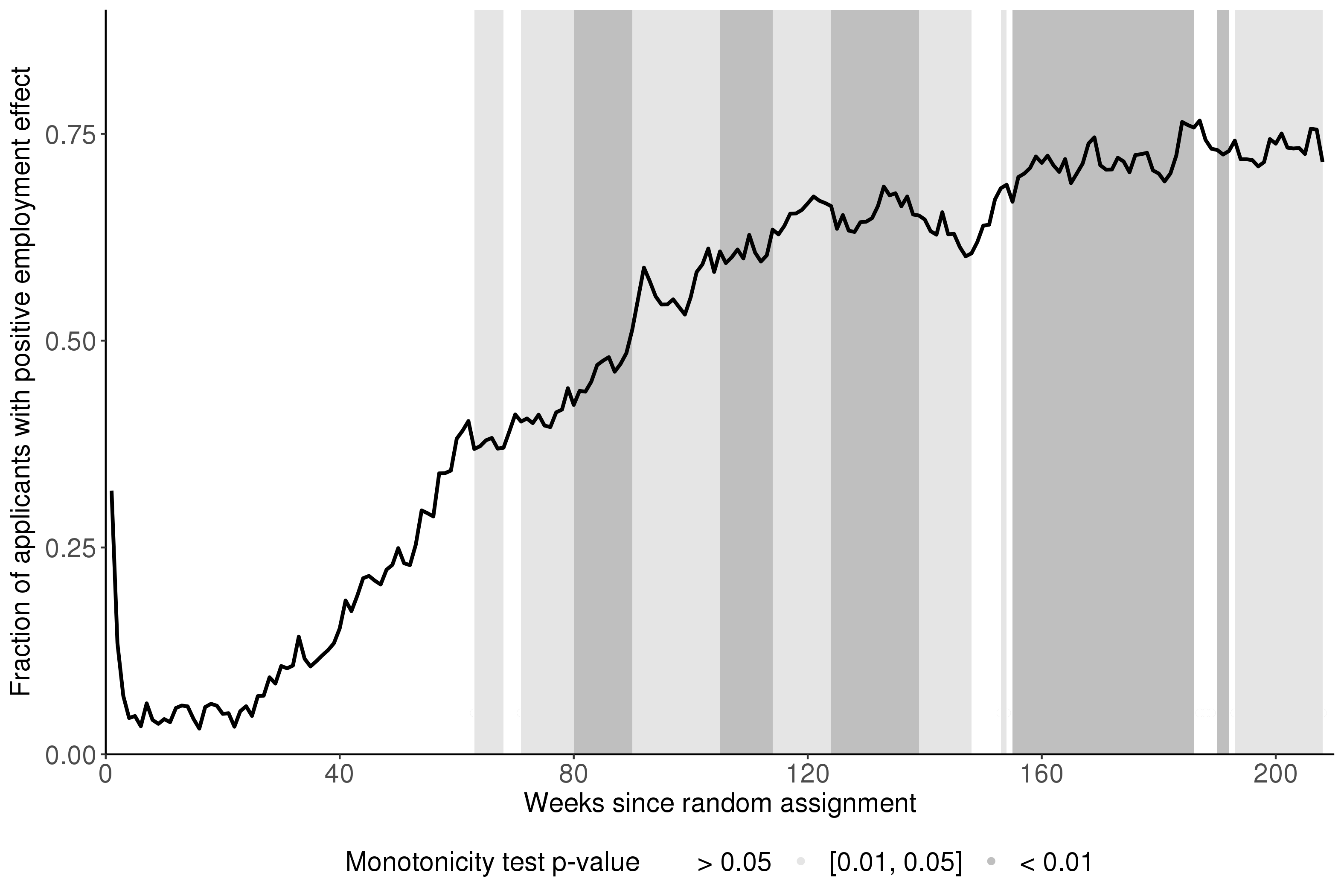
Figure 1: Fraction of JobCorps applicants with positive conditional employment effect by week.

Notes. The horizontal axis shows the number of weeks since random assignment. The vertical axis shows the fraction of applicants whose conditional employment effect $\tau(x)$ is positive. Following week 60, a week is shaded if the test statistic $T$ exceeds the critical value at the $p=0.01$ (dark gray) or $p\in[0.05,0.01)$ (light gray) significance level. For each week, $\tau(x)$ is defined in equation (A.1) and estimated as in equation (6.2), the null hypothesis is as in equation (6.3), the test statistic $T$ is as in equation (6.4), and the test cells and critical values are as defined in Table A.4. Computations use design weights.

Table 1: Estimated bounds on the JobCorps effect on log wages under monotonicity.

	Basic	Covariate-based
	(1)	(2)
Week 45	[-0.072, 0.140]	[-0.074, 0.127]
	(-0.097, 0.170)	(-0.096, 0.156)
Week 90	[0.048, 0.049]	[0.036, 0.048]
	(0.011, 0.081)	(0.011, 0.075)
Week 208	[-0.020, 0.095]	[-0.014, 0.084]
	(-0.050, 0.118)	(-0.041, 0.109)
Covariates	N/A	5

Notes. The sample $(N=9,145)$ and the time horizons are the same as in Lee, (2009). Each panel reports estimated bounds (first row), the $95\%$ confidence region for the identified set (second row) and the $95\%$ Imbens and Manski, (2004) confidence interval for the true parameter (third row). Column (1) reports basic Lee bounds. Column (2) reports covariate-based Lee bounds. All bounds assume that JobCorps discourages employment in week 45 and helps employment following week 90. The covariate in Column (2) is a linear combination of $28$ baseline covariates, selected by Lee, given in Table B.1. The covariates are weighted by the coefficients from a regression of week 208 wages on all baseline characteristics in the control group. The five discrete groups are formed according to whether the predicted wage is within intervals defined by $\$6.75$, $\$7$, $\$7.50$, and $\$8.50$. Week 90 is highlighted in bold as the only week where Lee found a statistically significant effect on wages. Computations use design weights.

Table 1 replicates Lee’s estimates of basic (Column (1)) bounds on JobCorps effect on the wages of always-takers focusing on week 90. Week 90 is a special week since it is the first week where the average employment effect switches from negative to positive, and the only one out of five horizons where Lee found the average wage effect on the always-takers to be significant. In addition, I also compute the covariate-based bounds using the discretized predicted wage potential covariate that Lee proposed (Column (2)). Week 90 is the only horizon where Lee found JobCorps effect on wages to be statistically significant. However, basic Lee bounds do not overlap with the covariate-based ones. Sharpness fails because one of the five covariate-specific trimming thresholds exceeds $1$ and is being capped at $0.999$ to impose unconditional monotonicity. Capping corresponds to the researcher’s belief that the covariate-specific threshold exceeded $1$ due to sampling noise, the only belief consistent with unconditional monotonicity. Once this assumption is weakened, basic Lee bounds do not cover zero in any week (Table 7, Column 1).

Table 7 reports generalized Lee bounds on the JobCorps week 90 wage effect on the always-takers and the confidence region for the identified set. The no-covariate generalized Lee bounds cannot determine the direction of the effect (Column (1)). Neither can the bounds defined conditional on a subset of the covariates selected by Lee (Column (2)). If few of the covariates affect week 90 employment and wage, the Column (3) bounds suggest that JobCorps raises week 90 wages by $4.0$–$4.6\%$ on average, which is slightly smaller than Lee’s original estimate ($4.9$–$5\%$). Despite numerical proximity, Lee’s basic estimates (Table 1, Column 1) and generalized Lee estimates (Table 7, Column 3) have substantially different reasons for being tight. Lee’s estimates are tight because one believes JobCorps’s week 90 employment effect is close to zero. In contrast, the generalized bounds are tight because variation in employment is well-explained by reasons for joining JobCorps, highest grade completed, and variation in wages is explained by pre-randomization earnings, household income, gender and other socio-economic factors.

The sparsity assumption of Column (3) may not be economically plausible. In Column (4), the target bounds are defined as the generalized Lee bounds given the $15$ covariates, selected for either employment or wage equation in Column (3). The Column (4) are almost the same as the Column (3) ones, suggesting that the bounds are not too sensitive to sparsity violations. However, the Column (4) confidence region does not account for the uncertainty in how these $15$ covariates are selected.

Figure 2 reports the upper and lower bounds on the average log wage for the always-takers in the control status, $\mathbb{E}[Y_{\text{week}}(0)|S_{\text{week}}(1)=S_{\text{week}}(0)=1]$ for each week. The lower (upper) bound grows from $1.45$ ($1.90$) in week $5$ to $1.978$ ($2.036$) in week $208$. The bounds’ width decreases from $0.45$ in week 14 to $0.01$ in week 208. The gap between the lower and the upper bound shrinks over time as the share of applicants with a positive employment effect, where the average log wage is identified in the control status, increases. One can interpret Figure 2 as corroborating the Ashenfelter, (1978) pattern and showing that earnings would have recovered even without JobCorps training. Therefore, evaluating JobCorps would have been very difficult without a randomized experiment, as one would need to explicitly model mean reversion in the potential wage in the control status.

7 Conclusion

Lee bounds are a popular empirical strategy for addressing post-randomization selection bias. This paper generalizes Lee bounds under conditional monotonicity. This relaxation is especially important for JobCorps job training program, where the standard (unconditional) monotonicity is unlikely to hold. Next, the paper proposes asymptotic theory for sharp bounds based on modern regularized techniques, and the proposed bounds are sharp in low-dimensional smooth and high-dimensional sparse designs. In the JobCorps, the use of additional covariates not considered by Lee, (2009) substantially tightens the bounds on the causal parameter.

The paper leaves a number of theoretical limitations and unresolved empirical questions. In terms of the theory, Assumption 2(a) is untestable. Yet, untestable does not mean true, which calls for more research on Lee bounds without (any) monotonicity. Next, Assumption 3(SEP) abstracts away from misclassification mistakes. Particularly, it rules out continuous covariates whose support is non-empty in both regions of positive and negative selection response. Second, Assumption 3 (REG) limits the attention only to continuously distributed outcomes with well-behaved densities. While this assumption is plausible for wage in the JobCorps data, it rules out binary outcomes commonly occur in survey samples (e.g., Finkelstein et al., (2012)).

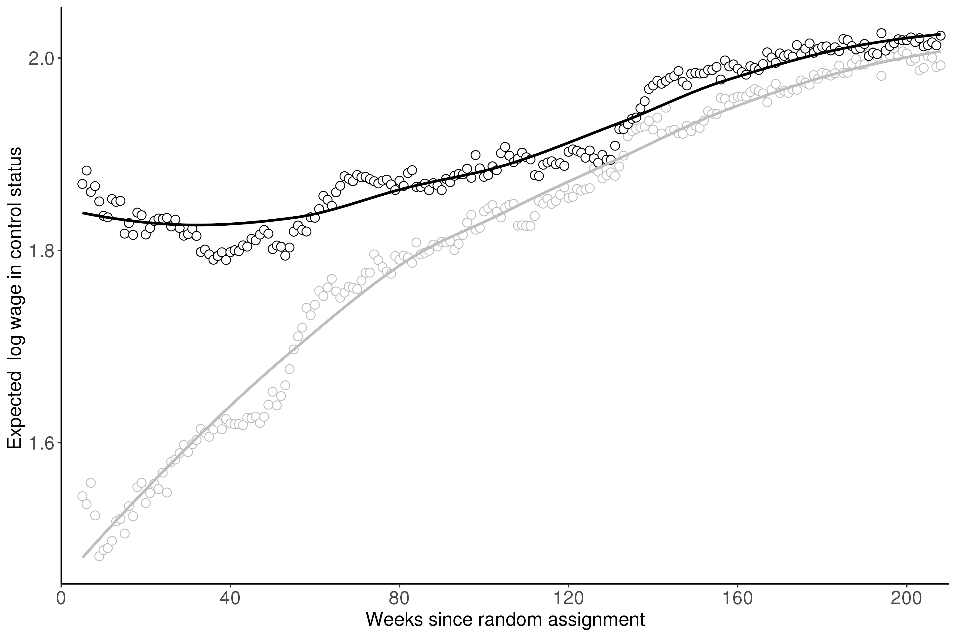
Figure 2: Estimated bounds on the average wage in the control status by week.

Notes. The horizontal axis shows the number of weeks since random assignment. The black (gray) circles show the upper (lower) bound on the average untreated log wage for the always-takers. The black (gray) fitted line is estimated by local linear approximation to $201$ black (gray) points, respectively. Computations use design weights.

Table 2: Estimated bounds on the JobCorps effect on week 90 log wages

	(1)	(2)	(3)	(4)
	[-0.027, 0.111]	[-0.005, 0.091]	[0.040, 0.046]	[0.041, 0.059]
	(-0.058, 0.142)	(-0.054, 0.135)	(0.001, 0.078)	(-0.019, 0.112)
Selection covs	28	28	5 177	15
Post-lasso-log.	N/A	N/A	9	N/A
Wage covs	0	28	470	15
Post-lasso	N/A	N/A	6	N/A

Notes. Estimated bounds are in square brackets and the $95\%$ confidence region for the identified set is in parentheses. All subjects are partitioned into the sets $\mathcal{X}_{\text{help}}=\{\widehat{p}(X)<1\}$ and $\mathcal{X}_{\text{hurt}}=\{\widehat{p}(X)>1\}$, where the trimming threshold $\widehat{p}(x)=\widehat{s}(0,x)/\widehat{s}(1,x)$ is estimated as in equation (6.2). (1): no-covariate bounds given $28$ Lee’s covariates. (2): generalized Lee bounds given $28$ Lee’s covariates. (3): generalized bounds given all covariates assuming few of them affect employment and wage. (4): generalized bounds given the union of raw covariates selected for the employment and wage equations in Column (3). Covariates are defined in Section A.4. Computations use design weights.

Appendix A: Proofs

A.1 Notation, Definitions, and Technical Lemmas

Notation and Definitions.

Define the conditional average treatment effect on selection as

$$\tau_{0}(x):=s_{0}(1,x)-s_{0}(0,x)$$ (A.1)

and the following sets

$$\mathcal{X}_{\text{help}}:=\{x:\tau_{0}(x)>0\},\quad\mathcal{X}_{\text{hurt}}:=\{x:\tau_{0}(x)<0\}.$$ (A.2)

The propensity score is

$$\mu_{1}(X)=\Pr(D=1\mid X),\quad\mu_{0}(X)=1-\mu_{1}(X)=\Pr(D=0\mid X).$$ (A.3)

The conditional CDF is defined as

$$F^{d}(t\mid x):=\Pr(Y\leq t\mid S=1,D=d,X=x),\quad d\in\{1,0\},\quad t\in\mathrm{R},$$

the conditional densities are

$$f^{d}(t|x)=f_{Y\mid S=1,D=d,X=x}(t\mid x),\quad d\in\{1,0\},\quad t\in\mathrm{R}.$$

The conditional quantiles in the selected treated and selected control groups are

$$Q^{d}(u,x):\quad\Pr(Y\leq Q^{d}(u,x)|S=1,D=d,X=x)=u,\quad u\in[0,1],\quad d\in\{1,0\}.$$ (A.4)

For $x\in\mathcal{X}_{\text{help}}$, the conditional upper bound is

$$\bar{\beta}_{U}^{\text{help}}(x)=\mathbb{E}[Y|D=1,S=1,Y\geq Q^{1}(1-p_{0}(x),x),X=x]-\mathbb{E}[Y|D=0,S=1,X=x]$$ (A.5)

and the conditional lower bound is

$$\bar{\beta}_{L}^{\text{help}}(x)=\mathbb{E}[Y|D=1,S=1,Y\leq Q^{1}(p_{0}(x),x),X=x]-\mathbb{E}[Y|D=0,S=1,X=x].$$ (A.6)

For $x\in\mathcal{X}_{\text{hurt}}$, the conditional upper bound is

$$\bar{\beta}_{U}^{\text{hurt}}(x)=\mathbb{E}[Y|D=1,S=1,X=x]-\mathbb{E}[Y|D=0,S=1,Y\leq Q^{0}(1/p_{0}(x),x),X=x]$$ (A.7)

and the conditional lower bound is

$$\bar{\beta}_{L}^{\text{hurt}}(x)=\mathbb{E}[Y|D=1,S=1,X=x]-\mathbb{E}[Y|D=0,S=1,Y\geq Q^{0}(1-1/p_{0}(x),x),X=x].$$ (A.8)

The sharp Lee bounds $\beta_{L}$ and $\beta_{U}$ are:

$$\beta_{\star} =\dfrac{\int_{\mathcal{X}}\beta_{\star}(x)\min(s(0,x),s(1,x))f_{X}(x)dx}{\int_{\mathcal{X}}\min(s(0,x),s(1,x))f_{X}(x)dx}\quad\star\in\{L,U\}.$$ (A.9)

The numerator’s moment function for the upper bound is in (3.8). For the lower bound, the moment function is

$$m_{L}(W,\xi)=1\{p(X)\leq 1\}m^{\text{help}}_{L}(W,\xi)+1\{p(X)>1\}m^{\text{hurt}}_{L}(W,\xi)$$

where

$$m^{\text{help}}_{L}(W,\xi) =\dfrac{D}{\mu_{1}(X)}\cdot S\cdot Y\cdot 1{\{Y\leq Q^{1}(p(X),X)\}}-\dfrac{1-D}{\mu_{0}(X)}\cdot S\cdot Y$$ (A.10)

$$m^{\text{hurt}}_{L}(W,\xi) =\dfrac{D}{\mu_{1}(X)}\cdot S\cdot Y-\dfrac{1-D}{\mu_{0}(X)}\cdot S\cdot Y\cdot 1{\{Y\geq Q^{0}(1-1/p(X),X)\}}.$$ (A.11)

The correction term for the upper bound is as follows. For $p(X)<1$, the correction term is given in (4.7). For $p(X)>1$, the correction term is

$$\text{cor}_{U}(W,\xi)=-Q^{0}(1/p(X),X)\bigg{(}\dfrac{1-D}{\mu_{0}(X)}(1/p(X))\cdot(S-s(0,X))$$ (A.12)

$$-\dfrac{D}{\mu_{1}(X)}\cdot(S-s(1,X))$$

$$-\dfrac{(1-D)S}{\mu_{0}(X)}Q^{0}(1/p(X),X)(1\{Y\leq Q^{0}(1/p(X),X)\}-1/p(X))\bigg{)}.$$

For the lower bound, the correction term is

$$\text{cor}_{L}(W,\xi) =Q^{1}(p(X),X)\bigg{(}\dfrac{1-D}{\mu_{0}(X)}\cdot(S-s(0,X))$$ (A.13)

$$-\dfrac{D}{\mu_{1}(X)}\cdot p(X)\cdot(S-s(1,X))$$

$$+\dfrac{DS}{\mu_{1}(X)}(1\{Y\leq Q^{1}(p(X),X)\}-p(X))\bigg{)},\quad p(X)<1$$

and

$$\text{cor}_{L}(W,\xi)=-Q^{0}(1-1/p(X),X)\bigg{(}\dfrac{1-D}{\mu_{0}(X)}(1/p(X))\cdot(S-s(0,X))$$ (A.14)

$$-\dfrac{D}{\mu_{1}(X)}\cdot(S-s(1,X))$$

$$-\dfrac{(1-D)S}{\mu_{0}(X)}(1\{Y\leq Q^{0}(1-1/p(X),X)\}-1/p(X)+1)\bigg{)},\quad p(X)>1$$

The orthogonal moment takes the form

$$g_{L}(W,\xi)=m_{L}(W,\xi)+\text{cor}_{L}(W,\xi),\quad g_{U}(W,\xi)=m_{U}(W,\xi)+\text{cor}_{U}(W,\xi).$$ (A.15)

Lemma A.1 (Corollary 4.1 in Horowitz and Manski, (1995)).

Let $Y$ be a continuous random variable and a mixture of two random variables, with cdfs $M^{*}(y)$ and $N^{*}(y)$, and a known mixing proportion $p^{*}\in(0,1)$, so we have $F^{*}(y)=p^{*}M^{*}(y)+(1-p^{*})N^{*}(y)$. Let $G^{*}(y)$ be the cdf of $Y$ after truncating the $p^{*}$ lower tail of $Y$. Then,

$$\int_{-\infty}^{\infty}ydN^{*}(y)\leq\int_{-\infty}^{\infty}ydG^{*}(y).$$

Furthermore, $\int_{-\infty}^{\infty}ydG^{*}(y)$ is the sharp upper bound on $\int_{-\infty}^{\infty}ydN^{*}(y)$.

Lemma A.1 is a restatement of Corollary 4.1 in Horowitz and Manski, (1995).

Definition 3 (Selection Rate).

For $d\in\{1,0\}$, let $\{S^{d}_{N}\}_{N\geq 1}$ be a sequence of sets, such that the first-stage estimates $\widehat{s}(d,x)$ of the true function $s_{0}(d,x)$ belong to $S^{d}_{N}$ with probability at least $1-o(1)$. Define the rates

$$\sup_{d\in\{1,0\}}\sup_{s\in S^{d}_{N}}(\mathbb{E}(s(d,X)-s_{0}(d,X))^{2})^{1/2}: =s_{N}$$

$$\sup_{d\in\{1,0\}}\sup_{x\in\mathcal{X}}\sup_{s\in S^{d}_{N}}|s(d,x)-s_{0}(d,x)| =:s^{\infty}_{N}$$

$$\sup_{d\in\{1,0\}}\sup_{s\in S^{d}_{N}}\mathbb{E}|s(d,X)-s_{0}(d,X)|: =s^{1}_{N}$$

Furthermore, the sets $S^{d}_{N}$ consist only of the functions obeying $s(d,x)>\kappa/2$ for all $x\in\mathcal{X}$ and $d\in\{1,0\}$.

Definition 4 (Quantile Rate).

For $d\in\{1,0\}$, let $\{Q^{d}_{N}\}_{N\geq 1}$ be a sequence of sets, such that the first-stage estimates $\widehat{Q}^{d}(u,x)$ of the true function $Q^{d}(u,x)$ belong to $Q^{d}(u,x)$ with probability at least $1-o(1)$. Define the mean square and $L_{1}$ rates

$$\sup_{d\in\{1,0\}}\sup_{Q\in Q_{N}^{d}}\sup_{u\in U}(\mathbb{E}(Q^{d}(u,X)-Q^{d}_{0}(u,X))^{2})^{1/2}=:q_{N}$$

$$\sup_{d\in\{1,0\}}\sup_{Q\in Q_{N}^{d}}\sup_{u\in U}\mathbb{E}|Q^{d}(u,X)-Q^{d}_{0}(u,X)|=:q^{1}_{N}$$

Definition 5 (Nuisance Realization Set).

Let $\{S^{d}_{N}\}_{N\geq 1}$ and $\{Q^{d}_{N}\}_{N\geq 1}$ be the sequences of sets in Definitions 3 and 4, and let $\xi(x)$ be as defined in (3.7). Then, the set $\Xi_{N}$ is taken as the cartesian product of the sets $S^{1}_{N},S^{0}_{N},Q^{1}_{N},Q^{0}_{N}$ that shrink towards $\xi_{0}(u,x):=\{s_{0}(1,x),s_{0}(0,x),Q^{1}_{0}(\cdot,x),Q^{0}_{0}(\cdot,x)\}$.

Lemma A.2 (Negligible First-Stage Error).

Let $R(W,\xi)$ be a known function of the data vector $W$ and the nuisance parameter $\xi_{0}$. Let $\{\Xi_{N}:N\geq 1\}$ be a sequence of sets that contain the first-stage estimate $\widehat{\xi}$ w.p. approaching one. The sets shrink at the following rates

$$\sup_{\xi\in\Xi_{N}}|\mathbb{E}[R(W,\xi)-R(W,\xi_{0})]|=O(B_{N})=o(N^{-1/2})$$

$$\sup_{\xi\in\Xi_{N}}(\mathbb{E}(R(W,\xi)-R(W,\xi_{0}))^{2})^{1/2}=O(V_{N})=o(1).$$

Then, $\sqrt{N}\mathbb{E}_{N}[R(W_{i};\widehat{\xi}_{i})-R(W_{i},\xi_{0})]=o_{P}(1)$.

Lemma A.2 is a special case of Lemma A.3 in Semenova and Chernozhukov, (2021) with the constant basis function $p(X)=1$.

Lemma A.3 (Lipschitz CDF implies Lipschitz quantile).

Let $\{F_{q}(\cdot),q\in\mathcal{S}^{d-1}\}$ be the CDF of $Y_{q}$ such that

$$\sup_{t\in\mathcal{R}}|F_{q_{1}}(t)-F_{q_{2}}(t)|\leq\bar{F}\|q_{1}-q_{2}\|$$ (A.16)

and the PDF such that

$$\inf_{q\in\mathcal{S}^{d-1}}\inf_{t\in\text{Conv}(Q_{q}(1-p),p\in U,q\in\mathcal{S}^{d-1})}|f_{q}(t)|\geq\bar{B}_{f}>0.$$

Then,

$$\sup_{q_{1},q_{2}\in\mathcal{S}^{d-1}}\sup_{p\in U}|Q_{q_{2}}(1-p)-Q_{q_{1}}(1-p)| \leq\sup_{t\in\mathcal{R}}|F_{q_{1}}(t)-F_{q_{2}}(t)|\sup_{t\in\mathcal{R}}\sup_{q\in\mathcal{S}^{d-1}}f_{q}^{-1}(t)$$

$$\leq\|q_{1}-q_{2}\|\bar{F}/\bar{B}_{f}.$$ (A.17)

Proof of Lemma A.3.

I use an implicit function theorem-type argument. By definition,

$$F_{q_{1}}(Q_{q_{1}}(1-p))=1-p,\quad F_{q_{2}}(Q_{q_{2}}(1-p))=1-p,$$

which implies

$$F_{q_{1}}(Q_{q_{1}}(1-p))-F_{q_{2}}(Q_{q_{2}}(1-p)) =F_{q_{1}}(Q_{q_{1}}(1-p))-F_{q_{2}}(Q_{q_{1}}(1-p))$$

$$+F_{q_{2}}(Q_{q_{1}}(1-p))-F_{q_{2}}(Q_{q_{2}}(1-p))=0.$$

Mean value theorem gives for some $t^{*}\in(Q_{q_{1}}(1-p),Q_{q_{2}}(1-p))$

$$|F_{q_{2}}(Q_{q_{1}}(1-p))-F_{q_{2}}(Q_{q_{2}}(1-p))|=f_{q_{2}}(t^{*})|Q_{q_{1}}(1-p))-Q_{q_{2}}(1-p)|,$$

and

$$|Q_{q_{1}}(1-p)-Q_{q_{2}}(1-p)|\leq\sup_{t}\sup_{t^{*}}\dfrac{|F_{q_{2}}(t)-F_{q_{2}}(t)|}{f_{q_{2}}(t^{*})}\leq\bar{F}\|q_{1}-q_{2}\|/\bar{B}_{f}.$$

Invoking (A.16) gives (A.3). ∎

ASSUMPTION A.2 (Concentration).

Let $\{R(W_{q},\xi),q\in\mathcal{S}^{d-1}\}$ be a known function of the data vector $W_{q}$ and the nuisance parameter $\xi_{0}(q)$. The following conditions hold for the function class

$$\mathcal{F}_{\xi} =\{g_{U}(W,\xi(q)),q\in\mathcal{S}^{d-1}\}$$ (A.18)

(1). There exists a measurable envelope function $F_{\xi}=F_{\xi}(W)$ that almost surely bounds all elements in the class $\sup_{q\in\mathcal{S}^{d-1}}|g_{U}(W,q,\xi(q))|\leq F_{\xi}(W)\quad\text{a.s.}$. There exists $c>2$ such that $\|F_{\xi}\|_{L_{P,c}}:=\left(\int_{w\in\mathcal{W}}(F_{\xi}(w))^{c}\right)^{1/c}<\infty$. There exist constants $a,v$ that may depend on $N$ such that the uniform covering entropy of the function class $\mathcal{F}_{\xi}$ is bounded

$$\log\sup_{Q}N(\epsilon\|F_{\xi}\|_{Q,2},\mathcal{F}_{\xi},\|\cdot\|_{Q,2})\leq v_{N}\log(a_{N}/\epsilon),\quad\text{ for all }0<\epsilon\leq 1.$$ (A.19)

and (5.16) holds. (2) For the true parameter value $\xi_{0}$, the function class $\mathcal{F}_{\xi_{0}}$ is $P$-Donsker, and (A.19) holds for some constant $v$ and $a$ that do not change with $N$.

Lemma A.4 (Negligible First-Stage Error).

Let $\{R(W_{q},\xi),q\in\mathcal{S}^{d-1}\}$ be a known function of the data vector $W_{q}$ and the nuisance parameter $\xi_{0}(q)$. Suppose the following conditions hold. (1) There exist sequences $B_{N}=o(N^{-1/2})$ and $V_{N}=o(1)$ such that

$$\sup_{\xi\in\Xi_{N}}\sup_{q\in\mathcal{S}^{d-1}}|\mathbb{E}[R(W_{q},\xi(q))-R(W_{q},\xi_{0}(q))]|=O(B_{N})=o(N^{-1/2})$$

$$\sup_{\xi\in\Xi_{N}}\sup_{q\in\mathcal{S}^{d-1}}(\mathbb{E}(R(W_{q},\xi(q))-R(W_{q},\xi_{0}(q)))^{2})^{1/2}=O(V_{N})=o(1).$$

(2) Assumption A.2 holds. Then, $\sup_{q\in\mathcal{S}^{d-1}}|\sqrt{N}\mathbb{E}_{N}[R(W_{qi};\widehat{\xi}_{i}(q))-R(W_{qi},\xi_{0}(q))]|=o_{P}(1)$.

Lemma A.4 follows from the Steps 2–5 of the proof of Theorem 3.1 in Semenova, (2023) as well as the maximal inequality (Lemma 6.2 in Chernozhukov et al., (2018)).

Lemma A.5 (Entropy Bounds).

(1) Let $Z(X)$ be a vector of basis functions. The function class

$$\mathcal{M} =\bigg{\{}W\rightarrow Z(X)^{\prime}\zeta,\quad\zeta\in\mathrm{R}^{p_{X}},\|\zeta\|_{0}\leq C_{X}s_{N},\|\zeta\|\leq C_{X}\bigg{\}}$$

obeys $a_{N}=p_{X}+N$,

$$\log\sup_{Q}N(\epsilon\|M\|_{Q,2},\mathcal{M},\|\cdot\|_{Q,2})\lesssim 1+s_{N}\log(a_{N}/\epsilon),\quad\text{ for all }0<\epsilon\leq 1.$$ (A.20)

(2) Suppose $\mathbf{Y}\in\mathrm{R}^{d}$ is a.s. bounded: $\|\mathbf{Y}\|\leq M\text{ a.s. }$ for some finite $M$. (2) There exists an integrable function $\bar{F}(x)$, so that

$$\sup_{t\in\mathrm{R}^{d}}|F_{q_{1}}(t\mid x)-F_{q_{2}}(t\mid x)|\leq\bar{F}(x)\|q_{1}-q_{2}\|$$

and $\inf_{q\in\mathcal{S}^{d-1}}\inf_{t\in\text{Conv}(Q_{q}(1-p),p\in U,q\in\mathcal{S}^{d-1})}|f_{q}(t)|\geq\bar{B}_{f}>0.$. Then, (A.19) holds with $v_{N}=d$ and $a_{N}$ that do not depend on $N$, and the function class $\mathcal{M}$

$$\mathcal{M}:=\{X\rightarrow Q_{Y_{q}}(p(X),X),\quad q\in\mathcal{S}^{d-1}\}$$

is a VC class.

Proof of Lemma A.5.

Invoking (A.3) gives

$$|Q_{q_{1}}(p_{0}(x),x)-Q_{q_{2}}(p_{0}(x),x)| \leq\bar{F}(x)/\bar{B}_{f}\|q_{1}-q_{2}\|$$ (A.21)

By Example 19.7 from van der Vaart, (2000), the covering numbers of the function class $\mathcal{M}$ obey

$$N_{[]}(\epsilon\|\bar{F}(x)/\bar{B}_{f}\|_{P,r},\mathcal{M},L_{r}(P))\lesssim\left(\dfrac{2}{\epsilon}\right)^{d},\text{ every }0<\epsilon<2.$$

Finally, since $\mathbf{Y}\in\mathrm{R}^{d}$ is an a.s. bounded vector, each element of the class $\mathcal{M}$ is bounded by $\|\mathbf{Y}\|\leq M\text{ a.s. }$, and $M$ can be taken as the envelope of $\mathcal{M}$. Therefore, $\mathcal{M}$ is $P$-Donsker and obeys (A.19) with $v=d$ and $a=2$.

∎

Lemma A.6 (Verification of Assumption A.2).

The class $\mathcal{F}_{\xi_{0}}=\{g_{U}(W_{q},\xi_{0}(q)),q\in\mathcal{S}^{d-1}\}$ is a VC class, that is, obeys (A.20) with $v$ and $a$ that do not change with $N$. Furthermore, the class $\mathcal{F}_{\xi}=\{g_{U}(W_{q},\xi(q)),q\in\mathcal{S}^{d-1}\}$ is a VC class, that is, obeys (A.20) with $v_{N}$ and $a_{N}$.

Proof of Lemma A.6.

Consider the class of true quantile functions

$$\mathcal{L}_{\xi_{0}}:=\bigg{\{}L(q,X),\quad q\in\mathcal{S}^{d-1}\bigg{\}}=:\{X\rightarrow Q_{Y_{q}}(p(X),X),\quad q\in\mathcal{S}^{d-1}\}$$

and the class of estimates

$$\mathcal{L}_{\xi}:=\bigg{\{}W\rightarrow Z(X)^{\prime}\zeta,\quad\zeta\in\mathrm{R}^{p_{X}},\|\zeta\|_{0}\leq C_{X}s_{N},\|\zeta\|\leq C_{X}\bigg{\}}$$

Step 1. The function class $\mathcal{H}^{\prime}_{\xi}=\bigg{\{}W\rightarrow Y_{q}-L(q,X),\quad q\in\mathcal{S}^{d-1}\bigg{\}}$ is the sum of 2 VC classes. Therefore, by Andrews, 1994a , $\mathcal{H}^{\prime}$ is a VC class itself. Therefore, the class of indicators

$$\mathcal{H}:=\bigg{\{}W\rightarrow 1{\{Y_{q}-L(q,X)\leq 0\}},\quad q\in\mathcal{S}^{d-1}\bigg{\}}.$$

is also a VC class with a constant envelope.

Step 3 . The function class

$$\mathcal{H}_{1}=\bigg{\{}W\rightarrow\dfrac{D\cdot S\cdot 1{\{Y_{q}\leq L(q,X)\}}}{\mu_{1}(X)}\bigg{\}}$$

is obtained by multiplying each element of $\mathcal{H}$ by an a.s. bounded random variable $D\cdot S/\mu_{1}(X)$. The function class

$$\mathcal{H}_{2}=\bigg{\{}W\rightarrow L(q,X)\left(\dfrac{(1-D)}{\mu_{0}(X)}-s(0,X\right)\bigg{\}}$$

is obtained from $\mathcal{M}$ by multiplying each element of $\mathcal{M}$ by an a.s. bounded random variable $\left(\dfrac{(1-D)}{\mu_{0}(X)}-s(0,X)\right)$. The same argument applies to the function class

$$\mathcal{H}_{3}=\bigg{\{}W\rightarrow L(q,X)p_{0}(X)\bigg{(}\dfrac{D}{\mu_{1}(X)}-s(1,X)\bigg{)}\bigg{\}}.$$

The function class

$$\mathcal{H}_{4}=\bigg{\{}W\rightarrow L(q,X)s(1,X)\left(\dfrac{D\cdot S1{\{Y_{q}\leq L(q,X)\}}}{\mu_{1}(X)s(1,X)}-p_{0}(X)\right)\bigg{\}}$$

is obtained as a product of function classes $\mathcal{M}$ and $\mathcal{H}$, multiplied by a random variable $s(1,X)$. Finally, the function class $\mathcal{F}_{\xi}$ in (A.18) is obtained by adding the elements of $\mathcal{H}_{k},\quad k=1,2,3,4$. Since entropies obey the rules of addition and multiplication by a random variable (Andrews, 1994a ), the argument follows.

∎

Proofs for Section 3

Proof of Lemma 1.

Step 1. For any $x\in\mathcal{X}_{\text{help}}$,

$$\Pr(S(1)=S(0)=1\mid X=x)=\Pr(S=1\mid X=x,D=0)=s(0,x).$$

Likewise, for any $x\in\mathcal{X}_{\text{hurt}}$,

$$\Pr(S(1)=S(0)=1\mid X=x)=\Pr(S=1\mid X=x,D=1)=s(1,x).$$

For any $x\in\mathcal{X}_{0}$, $\tau_{0}(x)=0\Rightarrow s_{0}(1,x)=s_{0}(0,x)$. Bayes rule for conditional density gives

$$f_{X}(x\mid S(1)=S(0)=1)=D_{0}^{-1}\begin{cases}s(0,x)f_{X}(x)&x\in\mathcal{X}_{\text{help}}\\ s(1,x)f_{X}(x)&x\in\mathcal{X}_{\text{hurt}},\\ s(1,x)f_{X}(x)&x\in\mathcal{X}_{0},\\ \end{cases}$$ (A.22)

where the denominator is

$$D_{0}:=\Pr(S(1)=S(0)=1) =\int_{\mathcal{X}_{\text{help}}}s(0,x)f_{X}(x)dx+\int_{\mathcal{X}_{\text{hurt}}}s(1,x)f_{X}(x)dx+\int_{\mathcal{X}_{0}}s(1,x)f_{X}(x)dx$$ (A.23)

$$=\int_{\mathcal{X}}\min(s(0,x),s(1,x))f_{X}(x)dx=\mathbb{E}\min(s(0,X),s(1,X)).$$ (A.24)

Step 2. By the law of conditional probability,

$$\Pr(Y\geq Q_{0}^{1}(1-p_{0}(x),x)\mid D=1,S=1,X=x)=1-(1-p_{0}(x))=p_{0}(x).$$

For any $x\in\mathcal{X}_{\text{help}}$,

$$\mathbb{E}[m^{\text{help}}_{U}(W,\xi_{0})\mid X=x]$$

$$=\mathbb{E}[Y1{\{Y\geq Q^{1}(1-p_{0}(X),X)\}}\mid D=1,S=1,X=x]s(1,x)$$ (A.25)

$$-\mathbb{E}[Y\mid D=0,S=1,X=x]s(0,x).$$

$$=\mathbb{E}[Y\mid Y\geq Q_{0}^{1}(1-p_{0}(x),x),D=1,S=1,X=x]p_{0}(x)s(1,x)$$ (A.26)

$$-\mathbb{E}[Y\mid D=0,S=1,X=x]s(0,x)=\beta^{\text{help}}_{U}(x)\min(s(0,x),s(1,x)).$$

For $x\in\mathcal{X}_{\text{hurt}}$, a similar argument gives

$$\mathbb{E}[m^{\text{hurt}}_{U}(W,\xi_{0})\mid X=x]$$

$$=\mathbb{E}[Y\mid D=1,S=1,X=x]s(1,x)$$

$$-\mathbb{E}[Y1{\{Y\leq Q^{0}(1/p_{0}(X),X)\}}\mid D=0,S=1,X=x]\min(s(0,x),s(1,x))$$

$$=\beta^{\text{hurt}}_{U}(x)s(1,x).$$

Finally, for $x\in\mathcal{X}_{0}$, $\beta_{U}(x)=\beta_{L}(x)=\beta_{0}(x)$, $s(0,x)=s(1,x)$, $\mathbb{E}[m_{U}(W,\xi_{0})\mid X=x]=\mathbb{E}[m_{L}(W,\xi_{0})\mid X=x]=\beta_{U}(x)\min(s(0,x),s(1,x)).$.

Step 3. The proof of sharpness is similar to Lee, (2009). Consider the following data generating process (d.g.p.). For each $x\in\mathcal{X}_{\text{help}}$, the always-takers’ treated outcomes comprise the top $p_{0}(x)=s(0,x)/s(1,x)$ quantile of the distribution of $Y\mid D=1,S=1,X=x$ in the treated selected group. For this group, $\beta_{0}(x)=\beta_{U}(x)$ holds by Lemma A.1. Likewise, for each $x\in\mathcal{X}_{\text{hurt}}$, the always-takers’ untreated outcomes comprise the bottom $1/p(x)$-quantile of the distribution of $Y\mid D=0,S=1,X=x$ in the untreated selected group. For this group, $\beta_{0}(x)=\beta_{U}(x)$. Finally, for $x\in\mathcal{X}_{0}$, $\beta_{L}(x)=\beta_{U}(x)$, which implies $\beta_{L}(x)=\beta_{0}(x)=\beta_{U}(x)$. Therefore, the largest attainable value of $\mathbb{E}[Y(1)-Y(0)\mid S(1)=S(0)=1]$ is

$$\int_{\mathcal{X}}\beta_{U}(x)f_{X}(x\mid S(1)=S(0)=1)dx.$$

Since the conditional density $f_{X}(x\mid S(1)=S(0)=1)$ is identified in (A.22), the statement holds. That is, for any $\beta^{\prime}<\beta_{U}$, $\beta^{\prime}$ cannot be a valid bound because there exists a d.g.p. for which $\beta_{0}=\beta_{U}>\beta^{\prime}$. ∎

A.2 Proofs for Section 4

Define

$$\psi_{4}(1): =\dfrac{DS}{\mu_{1}(X)}b^{1}_{1}(X)\left(1\{Y\leq b^{1}_{1}(X)\}-(1-p(X))\right)$$ (A.27)

$$\psi_{5}(1): =b^{0}_{2}(X)\dfrac{(1-D)}{\mu_{0}(X)}\left(S-s(0,X)\right)$$ (A.28)

$$\psi_{6}(1): =b^{0}_{3}(X)p(X)\dfrac{D}{\mu_{1}(X)}\left(S-s(1,X)\right)$$ (A.29)

$$\psi_{7}(1): =(b^{1}_{1}(X)-b^{0}_{2}(X))\dfrac{(1-D)}{\mu_{0}(X)}\left(S-s(0,X)\right)$$ (A.30)

$$\psi_{8}(1): =(b^{1}_{1}(X)-b^{0}_{2}(X))\dfrac{D}{\mu_{1}(X)}\left(S-s(1,X)\right)$$ (A.31)

$$\psi_{9}(1): =(b^{0}_{2}(X)-b^{0}_{3}(X)))\dfrac{D}{\mu_{1}(X)}\left(S-s(1,X)\right)$$ (A.32)

$$\psi_{4}(0): =b^{0}_{3}(X)\dfrac{DS}{\mu_{1}(X)}\left(1\{Y\leq b^{0}_{3}(X)\}-(1-p_{0}(X))\right)$$ (A.33)

$$\psi_{5}(0): =b^{0}_{3}(X)\dfrac{(1-D)}{\mu_{0}(X)}\left(S-s_{0}(0,X)\right)$$ (A.34)

$$\psi_{6}(0): =b^{0}_{3}(X)p_{0}(X)\dfrac{D}{\mu_{1}(X)}\left(S-s_{0}(1,X)\right)$$ (A.35)

Lemma A.7 (Verification of small bias condition).

Under Assumptions 3 and 4,

$$\sup_{\xi\in\Xi_{N}}|\mathbb{E}(g_{U}(W,\xi)-g_{U}(W,\xi_{0}))|=O(s_{N}^{2}+q_{N}^{2})$$ (A.36)

$$\sup_{\xi\in\Xi_{N}}\mathbb{E}(g_{U}(W,\xi)-g_{U}(W,\xi_{0}))^{2}=O(s^{1}_{N}+q^{1}_{N}+s_{N}^{2}+q_{N}^{2})$$ (A.37)

Proof of Lemma A.7.

Step 1. Definitions Let $r\in(0,1)$ be a parameter

$$b^{r}_{1}(x) =Q_{r}(1-p(x),x)=Q_{0}(1-p(x),x)+r(Q(1-p(x),x)-Q_{0}(1-p(x),x))$$

$$b^{r}_{2}(x) =Q_{0}(1-s_{r}(0,x)/s(1,x),x),\quad s_{r}(0,x)=s_{0}(0,x)+r(s(0,x)-s_{0}(0,x))$$

$$b^{r}_{3}(x) =Q_{0}(1-s_{0}(0,x)/s_{r}(1,x),x),\quad s_{r}(1,x)=s_{0}(1,x)+r(s(1,x)-s_{0}(1,x))$$

By construction, $b^{0}_{1}(x)=b^{1}_{2}(x)$ and $b^{0}_{2}(x)=b^{1}_{3}(x)$. For $k=1,2,3$, define

$$\psi_{k}(r): =\dfrac{DS}{\mu_{1}(X)}Y1\{Y\geq b^{r}_{k}(X),X)\}.$$

Since $\psi_{1}(0)=\psi_{2}(1)$ and $\psi_{2}(0)=\psi_{3}(1)$,

$$m^{\text{help}}_{U}(W,\xi)-m^{\text{help}}_{U}(W,\xi_{0}) =\sum_{k=1}^{3}[\psi_{k}(1)-\psi_{k}(0)].$$

Observe that

$$\text{cor}^{\text{help}}_{U}(W,\xi)-\text{cor}^{\text{help}}_{U}(W,\xi_{0}) =\sum_{k=4}^{6}[\psi_{k}(1)-\psi_{k}(0)]+\sum_{k=7}^{9}\psi_{k}(1)$$

$$g^{\text{help}}_{U}(W,\xi)-g^{\text{help}}_{U}(W,\xi_{0}) =\sum_{k=1}^{6}[\psi_{k}(1)-\psi_{k}(0)]+\sum_{k=7}^{9}\psi_{k}(1).$$

Step 2. Intermediate value theorem. For $r\in(0,1)$ and $x\in\mathcal{X}$, define the following functions

$$\Gamma_{1}(r,x): =yf_{11}^{1}(y\mid x)\bigg{|}_{y=b^{r}_{1}(x)}.$$

$$\Gamma_{2}(r,x): =y^{2}f_{11}^{1}(y\mid x)\bigg{|}_{y=b^{r}_{1}(x)}.$$

$$\zeta(r,x) =\partial_{r}\Gamma_{1}(r,x):=(f_{11}^{1}(y\mid x)+y\partial_{y}f_{11}^{1}(y\mid x))\bigg{|}_{y=b^{r}_{1}(x)}.$$

$$\mathbb{E}[\psi_{k}(1)-\psi_{k}(0)\mid X=x] =-s_{0}(1,x)\int_{b^{1}_{k}(x)}^{b^{0}_{k}(x)}yf_{11}^{1}(y\mid x)dy$$

$$\mathbb{E}[(\psi_{k}(1)-\psi_{k}(0))^{2}\mid X=x] =s_{0}(1,x)\bigg{|}\int_{b^{1}_{k}(x)}^{b^{0}_{k}(x)}y^{2}f_{11}^{1}(y\mid x)dy\bigg{|}$$

For some $r_{1}=r_{1}(x)$, $r_{2}=r_{2}(x)$ and $r_{3}=r_{3}(x)$, intermediate value theorem gives bounds for the first order terms

$$\mathbb{E}[\psi_{1}(1)-\psi_{1}(0)\mid X=x] =s_{0}(1,x)\Gamma_{1}(r_{1}(x),x)(b^{1}_{1}(x)-b^{0}_{1}(x)).$$

$$\mathbb{E}[\psi_{2}(1)-\psi_{2}(0)\mid X=x] =s_{0}(1,x)/s(1,x)\cdot b_{2}^{r_{2}(x)}(x)\cdot(s(0,x)-s_{0}(0,x))$$

$$\mathbb{E}[\psi_{3}(1)-\psi_{3}(0)\mid X=x] =-s_{0}(1,x)/s(1,x)b_{3}^{r_{3}(x)}(x)\cdot(s(1,x)-s_{0}(1,x))\cdot p_{0}(x)$$

For the second powers, for some $r^{\prime}_{1}=r^{\prime}_{1}(x)$, $r^{\prime}_{2}=r^{\prime}_{2}(x)$ and $r^{\prime}_{3}=r^{\prime}_{3}(x)$,

$$\mathbb{E}[(\psi_{1}(1)-\psi_{1}(0))^{2}\mid X=x] =s_{0}(1,x)\Gamma_{2}(r^{\prime}_{1}(x),x)|b^{1}_{1}(x)-b^{0}_{1}(x)|.$$ (A.38)

$$\mathbb{E}[(\psi_{2}(1)-\psi_{2}(0))^{2}\mid X=x] =s_{0}(1,x)/s(1,x)\cdot b_{2}^{2r_{2}^{\prime}(x)}(x)\cdot|s(0,x)-s_{0}(0,x)|$$

$$\mathbb{E}[(\psi_{3}(1)-\psi_{3}(0))^{2}\mid X=x] =b_{3}^{2r_{3}^{\prime}(x)}(x)\cdot s_{0}(1,x)/s(1,x)\cdot p_{0}(x)\cdot|s(1,x)-s_{0}(1,x)|$$

For some $r_{4}=r_{4}(x)$ and $r_{5}=r_{5}(x)$, the following equalities hold

$$F^{1}{11}(b^{1}_{1}(x)\mid x)-F^{1}{11}(b^{0}_{1}(x)\mid x) =f^{1}(b^{r_{4}(x)}(x)\mid x)(b^{1}_{1}(x)-b^{0}_{1}(x))$$ (A.39)

$$b^{1}_{2}(x)-b^{0}_{2}(x) =f^{-1}(Q_{0}(1-s_{r_{5}(x)}(0,x)/s_{1}(1,x),x))(s(0,x)-s_{0}(0,x))s^{-1}(1,x)$$ (A.40)

$$b^{1}_{3}(x)-b^{0}_{3}(x) =f^{-1}(Q_{0}(1-s_{0}(0,x)/s_{r_{6}(x)}(1,x),x))(s(1,x)-s_{0}(1,x))p_{0}(x)s^{-1}(1,x)$$ (A.41)

Step 3.a. Bounding the bias $\psi_{1}(1)-\psi_{1}(0)+\psi_{4}(1)$.

$$\mathbb{E}[\psi_{4}(1)\mid X=x]=s_{0}(1,x)b^{1}_{1}(x)(F^{1}{11}(b^{1}_{1}(x)\mid x)-F^{1}{11}(b^{0}_{1}(x)\mid x))$$

$$=s_{0}(1,x)b^{1}_{1}(x)f_{11}^{1}(b^{r_{4}(x)}_{1}(x)\mid x)(b^{1}_{1}(x)-b^{0}_{1}(x))$$

$$=s_{0}(1,x)(b^{1}_{1}(x)-b^{r_{4}(x)}_{1}(x))f_{11}^{1}(b^{r_{4}(x)}_{1}(x)\mid x)(b^{1}_{1}(x)-b^{0}_{1}(x))$$

$$+s_{0}(1,x)\Gamma_{1}(r_{4}(x),x)(b^{1}_{1}(x)-b^{0}_{1}(x)).$$

Therefore,

$$|\mathbb{E}[\psi_{1}(1)-\psi_{1}(0)+\psi_{4}(1)\mid X=x]| \leq|(\Gamma_{1}(r_{4}(x),x)-\Gamma_{1}(r_{1}(x),x))(b_{1}^{1}(x)-b_{1}^{0}(x))|$$

$$+|f_{11}^{1}(b^{r_{4}(x)}_{1}(x)\mid x)(r_{4}(x)-r_{1}(x))(b^{1}_{1}(x)-b^{0}_{1}(x))^{2}|$$

$$\leq^{ii}(C_{f}+MC_{f^{\prime}})(b^{1}_{1}(x)-b^{0}_{1}(x))^{2}+C_{f}(b^{1}_{1}(x)-b^{0}_{1}(x))^{2}.$$

Step 3.b. Bounding the bias $\psi_{2}(1)-\psi_{2}(0)+\psi_{5}(1)$.

$$\mathbb{E}[\psi_{5}(1)\mid X=x] =b^{1}_{2}(x)(s_{0}(0,x)-s(0,x)).$$

Summing $\mathbb{E}[\psi_{2}(1)-\psi_{2}(0)\mid X=x]$ and $\mathbb{E}[\psi_{5}(1)\mid X=x]$ gives

$$|\mathbb{E}[\psi_{2}(1)-\psi_{2}(0)\mid X=x]+\mathbb{E}[\psi_{5}(1)\mid X=x]|$$

$$=|-b^{1}_{2}(x)(1-s_{0}(1,x)/s(1,x))(s(0,x)-s_{0}(0,x))$$

$$+(b^{1}_{2}(x)-b^{r_{2}(x)}_{2}(x))(s(0,x)-s_{0}(0,x))s_{0}(1,x)/s(1,x)|$$

$$=|-b^{1}_{2}(x)(s(1,x)-s_{0}(1,x))(s(0,x)-s_{0}(0,x))s^{-1}(1,x)$$

$$+(b^{1}_{2}(x)-b^{r_{2}(x)}_{2}(x))(s(0,x)-s_{0}(0,x))s_{0}(1,x)/s(1,x)|.$$

Invoking $|b^{0}_{1}(x)|\leq M$ and $s^{-1}(1,x)\leq 2/\kappa$ and

$$|b^{1}_{2}(x)-b^{r_{2}(x)}_{2}(x))|\leq B_{f}|(s(0,x)-s_{0}(0,x))|$$

$$|\mathbb{E}[\psi_{2}(1)-\psi_{2}(0)\mid X=x]+\mathbb{E}[\psi_{5}(1)\mid X=x]|$$

$$\leq 2(B_{f}+M)/\kappa((s(0,x)-s_{0}(0,x))^{2}+|(s(0,x)-s_{0}(0,x))(s(1,x)-s_{0}(1,x))|).$$

Step 3.c. Bounding the bias $\psi_{3}(1)-\psi_{3}(0)+\psi_{6}(1)$.

$$\mathbb{E}[\psi_{6}(1)\mid X=x] =-b^{1}_{3}(x)\cdot p(x)\cdot(s(1,x)-s_{0}(1,x)).$$

Summing $\mathbb{E}[\psi_{3}(1)-\psi_{3}(0)\mid X=x]$ and $\mathbb{E}[\psi_{6}(1)\mid X=x]$ gives

$$|\mathbb{E}[\psi_{3}(1)-\psi_{3}(0)\mid X=x]+\mathbb{E}[\psi_{6}(1)\mid X=x]|$$

$$=|b^{r_{3}(x)}_{3}(x)-b^{1}_{3}(x)|\cdot p_{0}(x)\cdot(s(1,x)-s_{0}(1,x))s_{0}(1,x)/s(1,x)$$

$$+b^{1}_{3}(x)(s(0,x)-s_{0}(0,x))\cdot(s(1,x)-s_{1}(0,x))s^{-1}(1,x)|$$

Step 3.d. Conclusion For $k=7,8$, the second-order correction terms obey

$$|\mathbb{E}(\psi_{k}(1)-\psi_{k}(0))|=|\mathbb{E}\psi_{k}(1)|\leq C(B_{f},\kappa)(\sup_{u\in U}(\mathbb{E}(Q(u,X)-Q_{0}(u,X))^{2})^{1/2}$$

$$+B_{f}\sup_{d\in\{1,0\}}{\mathbb{E}(s(d,X)-s_{0}(d,X))^{2}}^{1/2})$$

$$|\mathbb{E}\psi_{9}(1)|=|\mathbb{E}\psi_{9}(1)|\leq C(B_{f},\kappa)\sup_{d\in\{1,0\}}\mathbb{E}(s(d,X)-s_{0}(d,X))^{2}$$

$$\sup_{\xi\in\Xi_{N}}\sum_{k=1}^{9}\mathbb{E}[(\psi_{k}(1)-\psi_{k}(0))]=O(s^{2}_{N}+q^{2}_{N}).$$

Step 4. Bounding second powers Invoking (A.38) gives

Observe that

$$\psi_{4}(1)-\psi_{4}(0) =\dfrac{DS}{\mu_{1}(X)}(b^{1}_{1}(X)-b^{0}_{3}(X))\left(1\{Y\leq b^{1}_{1}(X)\}-(1-p(X))\right)$$

$$+\dfrac{DS}{\mu_{1}(X)}b^{0}_{3}(X)\left(1\{Y\leq b^{1}_{1}(X)\}-1\{Y\leq b^{0}_{3}(X)\}\right)$$

$$+\dfrac{DS}{\mu_{1}(X)}b^{0}_{3}(X)\left(p(X)-p_{0}(X)\right)=:I_{41}+I_{42}+I_{43}.$$

and

$$\psi_{5}(1)-\psi_{5}(0) =(b^{1}_{3}(X)-b^{0}_{3}(X))\dfrac{(1-D)}{\mu_{0}(X)}(S-s(0,X))$$

$$+b^{0}_{3}(X)\dfrac{(1-D)}{\mu_{0}(X)}(s_{0}(0,X)-s(0,X))=:I_{51}+I_{52}.$$

and

$$\psi_{6}(1)-\psi_{6}(0) =-(b^{1}_{3}(X)-b^{0}_{3}(X))p(X)\cdot\dfrac{D}{\mu_{1}(X)}\left(S-s(1,X)\right)$$

$$-b^{0}_{3}(X)(p(X)-p_{0}(X))\cdot\dfrac{D}{\mu_{1}(X)}\left(S-s(1,X)\right)$$

$$-b_{0}^{3}(X)p_{0}(X)\cdot\dfrac{D}{\mu_{1}(X)}\left(s_{0}(1,X)-s(1,X)\right)=:I_{61}+I_{62}+I_{63}.$$

Observe that

$$\mathbb{E}[(1\{Y\leq b^{1}_{1}(X)\}-1\{Y\leq b^{0}_{3}(X)\})^{2}\mid X=x]=|F(b^{1}_{1}(x))-F(b^{0}_{3}(x))|\leq C_{f}M^{2}/\kappa|b^{1}_{1}(x)-b^{0}_{3}(x)|.$$

Invoking (A.40)-(A.41) gives

$$|b^{1}_{1}(x)-b^{0}_{1}(x)| \leq\sup_{u\in U}|Q(u,x)-Q_{0}(u,x)|$$ (A.42)

$$|b^{1}_{2}(x)-b^{0}_{3}(x)| \leq\sum_{k=2}^{3}|b^{1}_{k}(x)-b^{0}_{k}(x)|\leq 4B_{f}/\kappa\sup_{d\in\{1,0\}}|s(d,x)-s_{0}(d,x)|$$ (A.43)

$$|p(x)-p_{0}(x)| \leq 2/\kappa(|s(0,x)-s_{0}(0,x)|+|s(1,x)-s_{0}(1,x)|).$$ (A.44)

Thus,

$$\sup_{\xi\in\Xi_{N}}\mathbb{E}[I^{2}_{42}]\leq\sup_{Q^{d}\in Q^{d}_{N}}\sup_{u\in U}\mathbb{E}|Q^{d}(u,X)-Q^{d}_{0}(u,X)|\leq q^{1}_{N}.$$

Let $k\in\{1,2,3\}$. For all terms $I_{4k},I_{5k},I_{6k}$ not $I_{42}$, the term is a product of a difference of functions of $X$, including $s(d,x)-s_{0}(d,x),\quad d\in\{1,0\}$ and (A.42)-(A.44) and a random variable that is bounded a.s. Therefore,

$$\sup_{\xi\in\Xi_{N}}\mathbb{E}I^{2}_{lk}\leq O(q^{2}_{N}+s^{2}_{N}),\quad l\in\{4,5,6\},k\{1,2,3\},\quad I_{lk}\neq I_{42}.$$

Step 5. Summary Steps 1-4 imply

$$\sup_{\xi\in\Xi_{N}}|\mathbb{E}(g_{U}(W,\xi)-g_{U}(W,\xi_{0}))|=O(s^{2}_{N}+q^{2}_{N}).$$

$$\sup_{\xi\in\Xi_{N}}\mathbb{E}(g_{U}(W,\xi)-g_{U}(W,\xi_{0}))^{2}=O(q^{1}_{N}+s^{1}_{N}+s^{2}_{N}+q^{2}_{N}).$$

∎

Proof of Theorem 1.

Step 1. Consider an open set $(\kappa/2,1-\kappa/2)\bigtimes(\kappa/2,1-\kappa/2)$. W.p. $1-o(1)$, the pair of estimated functions $(\widehat{s}(0,\cdot),\widehat{s}(1,\cdot))$ belongs to this set. The function $f(t_{1},t_{2})=t_{1}/t_{2}$ has bounded partial derivatives in any direction on this set. Invoking Assumptions 3 (SEP) and 4 gives that, w.p. $1-o(1)$, $\{X_{i}\}_{i=1}^{N}$ are correctly classified, and

$$\sqrt{N}(\mathbb{E}_{N}g_{D}(W_{i};\widehat{\tau}_{i})-g_{D}(W_{i},\tau_{0}))=o_{P}(1).$$

Step 2. By Lemma A.7, the first moments are bounded as

$$\sup_{\xi\in\Xi_{N}}|\mathbb{E}(g_{U}(W,\xi)-g_{U}(W,\xi_{0}))|=O(s_{N}^{2}+q_{N}^{2}).$$

and the second moments are bounded as

$$\sup_{\xi\in\Xi_{N}}\mathbb{E}(g_{U}(W,\xi)-g_{U}(W,\xi_{0}))^{2} \leq O(s_{N}^{1}+q_{N}^{1}+s^{2}_{N}+q^{2}_{N}).$$

Invoking Lemma A.2 with $B_{N}=s_{N}^{2}+q_{N}^{2}$ and $V^{2}_{N}=s_{N}^{1}+q_{N}^{1}+s^{2}_{N}+q^{2}_{N}$ gives $\sqrt{N}(\mathbb{E}_{N}g_{U}(W_{i};\widehat{\xi}_{i})-\mathbb{E}_{N}g_{U}(W_{i},\xi_{0}))=o_{P}(1)$. Step 3. Invoking Delta method for a continuous function

$$\psi(x,y,z):=(x/z,\quad y/z)^{\prime}$$

with $x=\mathbb{E}g_{L}(W,\xi_{0});y=\mathbb{E}g_{U}(W,\xi_{0});z=\mathbb{E}g_{D}(W,\tau_{0})>0$ gives the statement of the Theorem.

∎

A.3 Proofs for Section 5

Proof of Theorem 2.

Suppose $\sigma(q):\mathcal{S}^{d-1}\rightarrow\mathrm{R}$ is (1) convex, (2) positive homogenous of degree one and (3) lower-semicontinuous function of $q$. By Corollary 13.2.1 from Rockafellar, (1997), the properties (1)-(3) imply that $\mathcal{B}$ in (5.4) is a convex and compact set and $\sigma(q)$ is its support function. Steps 1-3 verify these properties for the trimming functional $q\rightarrow\sigma(q)$ in (5.3). Steps 4 shows that $\sigma(q)$ in (5.3) is differentiable if $Y\mid D=1,S=1$ is continuously distributed. Relying on Steps 1–4, Steps 5-6 verify the properties (1)–(3) and differentiability for $\sigma(q)$ in (5.5), which establishes Theorem 2.

Step 1. By construction, $q^{\prime}\beta_{0}=q^{\prime}\mathbb{E}[\mathbf{Y}(1)-\mathbf{Y}(0)\mid S(1)=S(0)=1]=\mathbb{E}[Y_{q}(1)-Y_{q}(0)\mid S(1)=S(0)=1]$, which coincides with the one-dimensional ATE in the model $(D,S,Y_{q})$. Invoking Lee bound for one-dimensional case gives

$$q_{1}^{\prime}\beta_{0}\leq\sigma(q_{1})\quad\text{ and }\quad q_{2}^{\prime}\beta_{0}\leq\sigma(q_{2}).$$

Let $\lambda\in[0,1]$. Multiplying the inequalities by $\lambda$ and $1-\lambda$ gives

$$(\lambda q_{1}+(1-\lambda)q_{2})^{\prime}\beta_{0}\leq\lambda\sigma(q_{1})+(1-\lambda)\sigma(q_{2}).$$

Next, take $q:=\lambda q_{1}+(1-\lambda)q_{2}$. By sharpness, $\sigma(\lambda q_{1}+(1-\lambda)q_{2})$ is the smallest bound on $(\lambda q_{1}+(1-\lambda)q_{2})^{\prime}\beta_{0}$ in the model without covariates. Therefore,

$$\sigma(\lambda q_{1}+(1-\lambda)q_{2})\leq\lambda\sigma(q_{1})+(1-\lambda)\sigma(q_{2}),$$

which implies that $\sigma(q)$ is a convex function of $q$.

Step 2. Let $\lambda>0$. Observe that the event $\{\lambda q^{\prime}\mathbf{Y}\geq Q_{\lambda q^{\prime}\mathbf{Y}}(u,X)\}$ holds if and only if $\{Y_{q}\geq Q_{Y_{q}}(u,X)\}$. Since $Y_{q}=Y_{q}$ is a linear function of $q$, $\sigma(q)$ defined in (5.7) is positive homogenous of degree $1$.

Step 3. Consider a sequence of vectors $q_{k}\rightarrow q,k\rightarrow\infty$. Suppose $\sigma(q_{k})\leq C$. Then, $q_{k}^{\prime}\beta_{0}\leq\sigma(q_{k})\leq C$, which implies that $q^{\prime}\beta_{0}\leq C$ must hold. Therefore, $C$ is a bound on $q^{\prime}\beta_{0}$. By sharpness, $\sigma(q)$ is the smallest bound on $q^{\prime}\beta_{0}$, which implies $\sigma(q)\leq C$.

Step 4. I show that $\sigma(q)$ is differentiable in $q$, which implies that $\mathcal{B}$ in (5.4) is strictly convex. Recall that $\gamma(q)$ is defined as

$$\gamma(q): =\mathbb{E}[Y\mid Y_{q}\geq Q^{1}{Y_{q}}(1-p_{0}),D=1,S=1]-\mathbb{E}[Y\mid D=0,S=1]$$

$$=p_{0}^{-1}\mathbb{E}[Y1\{Y_{q}\geq Q^{1}{Y_{q}}(1-p_{0})\}\mid D=1,S=1]-\mathbb{E}[Y\mid D=0,S=1].$$

Let $q_{1},q_{2}\in\mathcal{S}^{d-1}$. Define

$$G(q_{1},q_{2}): =\sigma(q_{2})-\sigma(q_{1})-\gamma(q_{1})^{\prime}(q_{2}-q_{1})$$

$$=p_{0}^{-1}\mathbb{E}[Y_{q_{2}}(1\{Y_{q_{2}}-Q^{1}{Y_{q_{2}}}(1-p_{0})\geq 0\}-1\{Y_{q_{1}}-Q^{1}{Y_{q_{1}}}(1-p_{0})\geq 0\})\mid D=1,S=1]$$

$$=p_{0}^{-1}\mathbb{E}[(Y_{q_{1}}-Q^{1}{Y_{q_{1}}}(1-p_{0}))(1\{Y_{q_{2}}-Q^{1}{Y_{q_{2}}}(1-p_{0})\geq 0\}-1\{Y_{q_{1}}-Q^{1}{Y_{q_{1}}}(1-p_{0})\geq 0\})\mid D=1,S=1]$$

$$+p_{0}^{-1}Q^{1}{Y_{q_{1}}}(1-p_{0})\mathbb{E}[(1\{Y_{q_{2}}-Q^{1}{Y_{q_{2}}}(1-p_{0})\geq 0\}-1\{Y_{q_{1}}-Q^{1}{Y_{q_{1}}}(1-p_{0})\geq 0\})\mid D=1,S=1]$$

$$=G_{1}(q_{1},q_{2})+G_{2}(q_{1},q_{2}).$$

The second term is zero by construction

$$G_{2}(q_{1},q_{2})=p_{0}^{-1}Q^{1}{Y_{q_{1}}}(1-p_{0})(p_{0}-p_{0})=0.$$

To bound the first term, I invoke the following bound

$$|1{\{x\geq z\}}-1{\{y\geq z\}}|\leq 1\{|z-y|<|x-y|\}$$ (A.45)

with $x:=Y_{q_{2}}-Q^{1}{Y_{q_{2}}}(1-p_{0})$ and $y:=Y_{q_{1}}-Q^{1}{Y_{q_{1}}}(1-p_{0})$ and $z:=0$. As a result,

$$|G(q_{1},q_{2})| \leq p_{0}^{-1}\mathbb{E}|Y_{q_{1}}-Q^{1}{Y_{q_{1}}}(1-p_{0})|1\{|Y_{q_{1}}-Q^{1}{Y_{q_{1}}}(1-p_{0})|$$

$$<|Y_{q_{2}}-Y_{q_{1}}-(Q^{1}{Y_{q_{2}}}(1-p_{0})-Q^{1}{Y_{q_{1}}}(1-p_{0}))|\}\mid D=1,S=1].$$

Invoking (A.3) from Lemma A.3 gives for $\bar{M}:=M+\bar{F}/\bar{B}_{f}$

$$|Y_{q_{2}}-Y_{q_{1}}-(Q^{1}{Y_{q_{2}}}(1-p_{0})-Q^{1}{Y_{q_{1}}}(1-p_{0}))| \leq\|q_{2}-q_{1}\|M+|(Q^{1}{Y_{q_{2}}}(1-p_{0})-Q^{1}{Y_{q_{1}}}(1-p_{0}))|$$

$$\leq\|q_{2}-q_{1}\|\bar{M}.$$

Therefore,

$$|G(q_{1},q_{2})| \leq p_{0}^{-1}\mathbb{E}[|Y_{q_{1}}-Q^{1}{Y_{q_{1}}}(1-p_{0})|1\{0\leq|Y_{q_{1}}-Q^{1}{Y_{q_{1}}}(1-p_{0})|<\bar{M}\|q_{2}-q_{1}\|\}\mid D=1,S=1]$$

$$\leq p_{0}^{-1}\bar{M}\|q_{2}-q_{1}\|\Pr(0\leq|Y_{q_{1}}-Q^{1}{Y_{q_{1}}}(1-p_{0}))|<\bar{M}\|q_{2}-q_{1}\|)$$

$$\leq p_{0}^{-1}\bar{M}\|q_{2}-q_{1}\|(F_{q_{1}}(Q^{1}{Y_{q_{1}}}(1-p_{0})+\bar{M}\|q_{2}-q_{1}\|)-F_{q_{1}}(Q^{1}{Y_{q_{1}}}(1-p_{0})-\bar{M}\|q_{2}-q_{1}\|))$$

$$=O(\|q_{2}-q_{1}\|^{2})=o(\|q_{1}-q_{2}\|),\quad q_{1}-q_{2}\rightarrow 0.$$

Step 5. The trimmed mean functions are

$$\beta(q,x)=\mathbb{E}[Y_{q}\mid Y_{q}\geq Q^{1}{Y_{q}}(1-p_{0}(x),x),D=1,S=1,X=x]-\mathbb{E}[Y_{q}\mid D=0,S=1,X=x]$$

and

$$\sigma(q)=\dfrac{\mathbb{E}_{X}\beta(q,X)s(0,X)}{\mathbb{E}s(0,X)}.$$

By construction, for each $x\in\mathcal{X}$, $\beta(q,x)$ is a convex and positive homogenous of degree one function of $q$. Therefore, a weighted average of these functions (with non-negative weighting function) must retain the properties.

Step 6. I invoke the argument of Step 5 conditional on covariates. Define

$$G(q_{1},q_{2},x): =\beta(q_{1},x)-\beta(q_{2},x)-\gamma(q_{1},x)^{\prime}(q_{2}-q_{1})=:G_{1}(q_{1},q_{2},x)+G_{2}(q_{1},q_{2},x),$$

where $G_{2}(q_{1},q_{2},x)=0$ for all $q_{1}$ and $q_{2}$. Invoking (5.9) gives

$$\sup_{q_{1},q_{2}\in\mathcal{S}^{d-1},x\in\mathcal{X}}|G(q_{1},q_{2},x)|=O(\|q_{2}-q_{1}\|^{2})=o(\|q_{1}-q_{2}\|),\quad q_{1}-q_{2}\rightarrow 0.$$

Therefore, $q\rightarrow\beta(q,x)$ is differentiable in $q$ almost surely in $\mathcal{X}$ with the gradient $\gamma(q,x)$. Note that $\sigma(q)$ in (5.5) reduces to

$$\sigma(q)=\dfrac{\int_{\mathcal{X}}\beta(q,x)s(0,x)f_{X}(x)dx}{\int_{\mathcal{X}}s(0,x)f_{X}(x)dx}=\dfrac{\mathbb{E}m_{U}(W_{q},\xi_{0}(q))}{\mathbb{E}s(0,X)}$$

The following dominance condition holds

$$\sup_{q\in\mathcal{S}^{d-1}}\|\gamma(q,x)\| =\sup_{q\in\mathcal{S}^{d-1}}\|\nabla_{q}\beta(q,x)\|\leq 2\bar{M},\quad\forall x\in\mathcal{X}.$$

By dominated conference theorem applies, the function

$$\partial_{q}\dfrac{\int_{\mathcal{X}}\beta(q,x)s(0,x)f_{X}(x)dx}{\int_{\mathcal{X}}s(0,x)f_{X}(x)dx}=\dfrac{\int_{\mathcal{X}}\partial_{q}\beta(q,x)s(0,x)f_{X}(x)dx}{\int_{\mathcal{X}}s(0,x)f_{X}(x)dx}=\dfrac{\int_{\mathcal{X}}\gamma(q,x)s(0,x)f_{X}(x)dx}{\int_{\mathcal{X}}s(0,x)f_{X}(x)dx}.$$

is differentiable (and, therefore, lower-hemicontinuous). Invoking Step 5 implies that $\sigma(q)$ in (5.5) obeys all 3 properties required for being a support function, and, furthermore, is differentiable.

∎

Proof of Theorem 3.

Invoking Lemma A.7 with $B_{N}:=s^{2}_{N}+q^{2}_{N}$ and $V_{N}^{2}=s^{1}_{N}+q^{1}_{N}+s_{N}+q_{N}$ verifies condition (1) in Lemma A.4. Assumption A.2 is verified in Lemma A.6. Invoking Lemma A.4 concludes the proof. ∎

Appendix B: Empirical details

A.4 JobCorps Data description.

In this section, I describe baseline covariates for the JobCorps empirical application. The data is taken from Schochet et al., (2008), who provides covariate descriptions in Appendix L. All covariates describe experiences before random assignment (RA). Most of the covariates represent answers to multiple choice questions; for these covariates I list the question and the list of possible answers. An answer is highlighted in boldface if is selected by post-lasso-logistic of Belloni et al., (2016) for one of employment equation specifications, described below. Table B.1 lists the covariates selected by Lee, (2009). A full list of numeric covariates, not provided here, includes $p=5,177$ numeric covariates.

Covariates selected by Lee, (2009). Lee, (2009) selected 28 baseline covariates to estimate parametric specification of the sample selection model. They are given in Table B.1.

Table B.1: Baseline covariates selected by Lee, (2009).

Name	Description
FEMALE	female
AGE	age
BLACK, HISP, OTHERRAC	race categories
MARRIED, TOGETHER, SEPARATED	family status categories
HASCHILD	has child
NCHILD	number of children
EVARRST	ever arrested
HGC	highest grade completed
HGC_MOTH, HGC_FATH	mother’s and father’s HGC
$\text{HH\_INC}1-\text{HH\_INC}5$	five household income groups with cutoffs $3,000,6,000,9,000,18,000$
$\text{PERS\_INC}1-\text{PERS\_INC}4$	four personal income groups with cutoffs $3,000,6,000,9,000$
WKEARNR	weekly earnings at most recent job
HRSWK_JR	ususal weekly work hours at most recent job
MOSINJOB	the number of months employed in past year
CURRJOB	employed at the moment of interview
EARN_YR	total yearly earnings
YR_WORK	any work in the year before RA

Reasons for joining JobCorps (R_X). Applicants were asked a question “How important was reason X on the scale from $1$ (very important) to $3$ (not important), or $4$ (N/A), for joining JobCorps?”. Each reason X was asked about in an independent question.

Table B.2: Reasons for joining JobCorps

Name	description	Name	description
R_HOME	getting away from home	R_COMM	getting away from community
R_GETGED	getting a GED	R_CRGOAL	desire to achieve a career goal
R_TRAIN	getting job training	R_NOWORK	not being able to find work

For example, a covariate R_HOME1 is a binary indicator for the reason R_HOME being ranked as a very important reason for joining JobCorps.

Sources of advice about the decision to enroll in JobCorps (IMP_X). Applicants were asked a question “How important was advice of X on the scale from $1$ (important) to $0$ (not important) ?”. Each source of advice was asked about in an independent question.

Table B.3: Sources of advice about the decision to enroll in JobCorps.

Name	description	Name	description
IMP_PAR	parent or legal guardian	IMP_FRD	friend
IMP_TCH	teacher	IMP_CW	case worker
IMP_PRO	probation officer	IMP_CHL	church leader

Main types of worry about joining JobCorps (TYPEWORR). Applicants were asked to select one main type of worry about joining JobCorps.

Table B.4: Types of worry about joining JobCorps

$\#$	description	$\#$	description
1	not knowing anybody or not fitting in	2	violence $/$ safety
3	homesickness	4	not knowing what it will be like
5	dealing with other people	6	living arrangements
7	strict rules and highly regimented life	8	racism
9	not doing well in classes	10	none

Drug use summary (DRUG_SUMP). Applicants were asked to select one of $5$ possible answers best describing their drug use in the past year before RA.

Table B.5: Summary of drug use in the year before RA

$\#$	description	$\#$	description
1	did not use drugs	2	marijuana $/$ hashish only
3	drugs other than marijuana $/$ hashish	4	both marijuana and other drugs

Frequency of marijuana use (FRQ_POT) . Applicants were asked to select one of $5$ possible answers best describing their marijuana $/$ hashish use in the past year before RA.

Table B.6: Frequency of marijuana/hashish use in the year before RA

$\#$	description	$\#$	description
1	daily	2	a few times each week
3	a few times each month	4	less often
5	missing	6	N/A

Applicant’s welfare receipt history. Applicants were asked whether they ever received food stamps (GOTFS), AFDC benefits (GOTAFDC) or other welfare (GOTOTHW) in the year prior to RA. In case of receipt, they asked about the duration of receipt in months ($\text{MOS\_ANYW},\text{MOS\_AFDC}$). For example, GOTAFDC=1 and MOS_AFDC=8 describes an applicant who received AFDC benefits during 8 months before RA.

Household welfare receipt history (WELF_KID). Applicants were asked about family welfare receipt history during childhood.

Table B.7: Family was on welfare when growing up

$\#$	description	$\#$	description
1	never	2	occasionally
3	half of the time	4	most or all time

Health status (HEALTH). Applicants were asked to rate their health at the moment of RA

Table B.8: Health status at RA

$\#$	description	$\#$	description
1	excellent	2	good
3	fair	4	poor

Arrest experience. CPAROLE21=1 is a binary indicator for being on probation or parole at the moment or RA. In addition, arrested applicants were asked about the time past since most recent arrest MARRCAT.

Table B.9: Number of months since most recent arrest

$\#$	description	$\#$	description
1	less than 12	2	12 to 24
3	24 or more	4	N/A

Table B.10: Figure 1 details: monotonicity test results

Weeks	Cell with the largest $t$-statistic	Average Test Statistic
(1)	(2)	(3)
Weeks 60 – 89	MOS_AFDC=8 or
PERS_INC=3 and EARN_YR $\in[720,3315]$	2.390
Weeks 90 – 116	R_HOME=1 and MARRCAT11=1 or
WELF_KID=4 and TYPEWORR=5	2.536
Weeks 117 – 152	R_COMM=1 and IMP_PRO=1 and FRQ_POT=3 or
DRG_SUMP=2 and TYPEWORR=5 and IMP_PRO=1	2.690
Weeks 153 – 186	IMP_PRO=1 and MARRCAT11 or
REASED_R4 = 1 and R_COMM=1 and DRG_SUMP=2	3.303
Weeks 187 – 208	same as weeks 90–116	2.221

Notes. This table shows the results for the monotonicity test in Figure 1. The test is conducted separately for each week using a week-specific test statistic and p-value. For each test, I partition $N=9,145$ subjects into $J=2$ cells $C_{1},C_{2}$. Column (2) describes the cell with the largest $t$-statistic whose value is compared to the critical value. Column (3) shows the average test-statistic across time period in Column (1). The test statistic is $T=\max_{j\in\{1,2\}}\widehat{\mu}_{j}/\widehat{\sigma}_{j}$, where $\widehat{\mu}_{j}$ and $\widehat{\sigma}_{j}$ are sample average and standard deviation of random variable $\xi_{j}:=\mathbb{E}[(2D-1)\cdot S|X\in C_{j}]$, weighted by design weights DSGN_WGT. The critical value $c_{\alpha}$ is the self-normalized critical value of Chernozhukov et al., (2019). For $\alpha=0.05$, $c_{\alpha}=1.960$. For $\alpha=0.01$, $c_{\alpha}=2.577$. Covariates are defined in Section A.4.

References

- Abdulkadiroglu et al., (2020) Abdulkadiroglu, A., Pathak, P. A., and Walters, C. R. (2020). Do parents value school effectiveness. American Economic Review, 110(5):1502–1539.
- Ackerberg et al., (2014) Ackerberg, D., Chen, X., Hahn, J., and Liao, Z. (2014). Asymptotic efficiency of semiparametric two-step gmm. Review of Economic Studies, 81:919–943.
- (3) Andrews, D. (1994a). Asymptotics for semiparametric econometric models via stochastic equicontinuity. Econometrica, 62(1):43–72.
- (4) Andrews, D. (1994b). Empirical process methods in econometrics. Econometrica, 1(62):43–72.
- Angrist et al., (2002) Angrist, J., Bettinger, E., Bloom, E., King, E., and Kremer, M. (2002). Vouchers for private schooling in colombia: Evidence from a randomized natural experiment. The American Economic Review, 92(5):1535–1558.
- Angrist et al., (2006) Angrist, J., Bettinger, E., and Kremer, M. (2006). Long-term consequences of secondary school vouchers: Evidence from administrative records in colombia. The American Economic Review, 96(3):847–862.
- Angrist et al., (2013) Angrist, J. D., Pathak, P. A., and Walters, C. R. (2013). Explaining charter school effectiveness. American Economic Journal: Applied Economics, 5(4):1–27.
- Ashenfelter, (1978) Ashenfelter, O. (1978). Estimating the effect of training programs on earnings. Review of Economics and Statistics, 60:47–50.
- Belloni and Chernozhukov, (2011) Belloni, A. and Chernozhukov, V. (2011). -penalized quantile regression in high-dimensional sparse models. The Annals of Statistics, 39(1):82–130.
- Belloni et al., (2019) Belloni, A., Chernozhukov, V., Chetverikov, D., and Fernandez-Val, I. (2019). Conditional quantile processes based on series or many regressors. Journal of Econometrics, 213(260):4–29.
- Belloni et al., (2017) Belloni, A., Chernozhukov, V., Fernandez-Val, I., and Hansen, C. (2017). Program evaluation and causal inference with high-dimensional data. Econometrica, 85:233–298.
- Belloni et al., (2016) Belloni, A., Chernozhukov, V., and Wei, Y. (2016). Post-selection inference for generalized linear models with many controls. Journal of Business & Economic Statistics, 34(4):606–619.
- Beresteanu and Molinari, (2008) Beresteanu, A. and Molinari, F. (2008). Asymptotic properties for a class of partially identified models. Econometrica, 76(4):763–814.
- Blanco et al., (2013) Blanco, G., Flores, C. A., and Flores-Lagunes, A. (2013). Bounds on average and quantile treatment effects of job corps training on wages. The Journal of Human Resources, 48(3):659–701.
- Bontemps et al., (2012) Bontemps, C., Magnac, T., and Maurin, E. (2012). Set identified linear models. Econometrica, 80:1129–1155.
- Bonvini and Kennedy, (2021) Bonvini, M. and Kennedy, E. H. (2021). Sensitivity analysis via the proportion of unmeasured confounding. Journal of the American Statistical Association, page 1–11.
- Bruns-Smith and Zhou, (2023) Bruns-Smith, D. and Zhou, A. (2023). Robust fitted-q-evaluation and iteration under sequentially exogenous unobserved confounders.
- Chandrasekhar et al., (2012) Chandrasekhar, A., Chernozhukov, V., Molinari, F., and Schrimpf, P. (2012). Inference for best linear approximations to set identified functions. arXiv e-prints, page arXiv:1212.5627.
- Chen and Flores, (2015) Chen, X. and Flores, C. A. (2015). Bounds on treatment effects in the presence of sample selection and noncompliance: The wage effects of job corps. Journal of Business and Economic Statistics, 33(4):523–540.
- Chernozhukov et al., (2018) Chernozhukov, V., Chetverikov, D., Demirer, M., Duflo, E., Hansen, C., Newey, W., and Robins, J. (2018). Double/debiased machine learning for treatment and structural parameters. Econometrics Journal, 21:C1–C68.
- Chernozhukov et al., (2019) Chernozhukov, V., Chetverikov, D., and Kato, K. (2019). Inference on causal and structural parameters using many moment inequalities. Review of Economic Studies, 86:1867–1900.
- Chernozhukov et al., (2016) Chernozhukov, V., Escanciano, J. C., Ichimura, H., Newey, W. K., and Robins, J. M. (2016). Locally Robust Semiparametric Estimation. arXiv e-prints, page arXiv:1608.00033.
- Chernozhukov et al., (2013) Chernozhukov, V., Fernandez-Val, I., and Melly, B. (2013). Inference on counterfactual distributions. Biometrics, 81(6):2205–2268.
- (24) Chernozhukov, V., Newey, W., and Singh, R. (2018a). Debiased machine learning of global and local parameters using regularized riesz representers. arXiv e-prints, page arXiv:1802.08667.
- (25) Chernozhukov, V., Newey, W. K., and Singh, R. (2018b). Automatic debiased machine learning of causal and structural effects. arXiv e-prints, page arXiv:1809.05224.
- Chernozhukov et al., (2010) Chernozhukov, V., Rigobon, R., and Stoker, T. (2010). Set identification and sensitivity analysis with Tobin regressors. Quantitative Economics, 1(6B):255 – 277.
- Chiang et al., (2019) Chiang, H. D., Kango, K., Ma, Y., and Sasaki, Y. (2019). Multiway cluster robust double/debiased machine learning.
- Chiang et al., (2019) Chiang, H. D., Kato, K., Ma, Y., and Sasaki, Y. (2019). Multiway Cluster Robust Double/Debiased Machine Learning. arXiv e-prints, page arXiv:1909.03489.
- Colangelo and Lee, (2020) Colangelo, K. and Lee, Y.-Y. (2020). Double Debiased Machine Learning Nonparametric Inference with Continuous Treatments. arXiv e-prints, page arXiv:2004.03036.
- Fan et al., (2019) Fan, Q., Hsu, Y.-C., Lieli, R. P., and Zhang, Y. (2019). Estimation of conditional average treatment effects with high-dimensional data. arXiv e-prints, page arXiv:1908.02399.
- Feller et al., (2016) Feller, A., Greif, E., Ho, N., Miratrix, L., and Pillai, N. (2016). Weak separation in mixture models and implications for principal stratification.
- Finkelstein et al., (2012) Finkelstein, A., Taubman, S., Wright, B., Bernstein, M., Gruber, J., Newhouse, J., Allen, H., Baicker, K., and Group, O. H. S. (2012). The oregon health insurance experiment: Evidence from the first year. Quarterly Journal of Economics, 127(3):1057–1106.
- Frangakis and Rubin, (2002) Frangakis, C. E. and Rubin, D. B. (2002). Principal stratification in causal inference. Biometrics, 58(1):21–29.
- Gafarov, (2019) Gafarov, B. (2019). Inference in high-dimensional set-identified affine models.
- Hardle and Stoker, (1989) Hardle, W. and Stoker, T. (1989). Investigating smooth multiple regression by the method of average derivatives. Journal of American Statistical Association, 84(408):986–995.
- Heiler, (2022) Heiler, P. (2022). Heterogeneous treatment effect bounds under sample selection with an application to the effects of social media on political polarization.
- Hirano et al., (2003) Hirano, K., Imbens, G., and Reeder, G. (2003). Efficient estimation of average treatment effects under the estimated propensity score. Econometrica, 71(4):1161–1189.
- Honore and Hu, (2020) Honore, B. and Hu, L. (2020). Selection without exclusion. Econometrica, 88(88):1007–1029.
- Horowitz and Manski, (1995) Horowitz, J. L. and Manski, C. F. (1995). Identification and robustness with contaminated and corrupted data. Econometrica, 63(2):281–302.
- Imbens and Manski, (2004) Imbens, G. and Manski, C. (2004). Confidence intervals for partially identified parameters. Econometrica, 72(6):1845–1857.
- Javanmard and Montanari, (2014) Javanmard, A. and Montanari, A. (2014). Confidence intervals and hypothesis testing for high-dimensional regression. Journal of Machine Learning Research, 2(4):2869–2909.
- Jeong and Namkoong, (2020) Jeong, S. and Namkoong, H. (2020). Robust causal inference under covariate shift via worst-case subpopulation treatment effects. arXiv e-prints, page arXiv:2007.02411.
- Kaido, (2017) Kaido, H. (2017). Asymptotically efficient estimation of weighted average derivatives with an interval censored variable. Econometric Theory, 33(5):1218–1241.
- Kaido et al., (2019) Kaido, H., Molinari, F., and Stoye, J. (2019). Confidence intervals for projections of partially identified parameters. Econometrica, 87(4):1397–1432.
- Kaido et al., (2021) Kaido, H., Molinari, F., and Stoye, J. (2021). Constraint qualifications in partial identification. Econometric Theory.
- Kaido and Santos, (2014) Kaido, H. and Santos, A. (2014). Asymptotically efficient estimation of models defined by convex moment inequalities. Econometrica, 82(1):387–413.
- Kallus and Zhou, (2019) Kallus, N. and Zhou, A. (2019). Assessing disparate impacts of personalized interventions: Identifiability and bounds.
- Kamat, (2019) Kamat, V. (2019). On the identifying content of instrument monotonicity.
- Kamat, (2021) Kamat, V. (2021). Identifying the effects of a program offer with an application to head start.
- Kline and Walters, (2019) Kline, P. and Walters, C. (2019). On heckits, late, and numerical equivalence. Econometrica, 87(2):677–696.
- Lee, (2009) Lee, D. (2009). Training, wages, and sample selection: Estimating sharp bounds on treatment effects. Review of Economic Studies, 76(3):1071–1102.
- Manski, (1989) Manski, C. F. (1989). Anatomy of the selection problem. The Journal of Human Resources, 24(3):343–360.
- Manski, (1990) Manski, C. F. (1990). Nonparametric bounds on treatment effects. The American Economic Review, 80(2):319–323.
- (54) Mogstad, M., Torgovitsky, A., and Walters, C. (2020a). The causal interpretation of two-stage least squares with multiple instrumental variables.
- (55) Mogstad, M., Torgovitsky, A., and Walters, C. (2020b). Policy evaluation with multiple instrumental variables.
- Molinari, (2020) Molinari, F. (2020). Chapter 5 - microeconometrics with partial identification. In Handbook of Econometrics, Volume 7A, volume 7 of Handbook of Econometrics, pages 355–486. Elsevier.
- Nekipelov et al., (2022) Nekipelov, D., Semenova, V., and Syrgkanis, V. (2022). Regularized orthogonal estimation of nonlinear semiparametric models.
- Newey, (1994) Newey, W. (1994). The asymptotic variance of semiparametric estimators. Econometrica, 62(6):245–271.
- Newey and Stoker, (1993) Newey, W. and Stoker, T. (1993). Efficiency of weighted average derivative estimators and index models. Econometrica, 61(5):1199–1223.
- Neyman, (1959) Neyman, J. (1959). Optimal asymptotic tests of composite statistical hypotheses. Probability and Statistics, 213(57):416–444.
- Neyman, (1979) Neyman, J. (1979). tests and their use. Sankhya, pages 1–21.
- Ning et al., (2020) Ning, Y., Peng, S., and Tao, J. (2020). Doubly robust semiparametric difference-in-differences estimators with high-dimensional data.
- Olma, (2021) Olma, T. (2021). Nonparametric estimation of truncated conditional expectation functions.
- Robins and Rotnitzky, (1995) Robins, J. and Rotnitzky, A. (1995). Semiparametric efficiency in multivariate regression models with missing data. Journal of American Statistical Association, 90(429):122–129.
- Robinson, (1988) Robinson, P. M. (1988). Root-n-consistent semiparametric regression. Econometrica, 56(4):931–954.
- Rockafellar, (1997) Rockafellar, R. T. (1997). Convex Analysis. Princeton University Press.
- Sasaki and Ura, (2020) Sasaki, Y. and Ura, T. (2020). Estimation and inference for Policy Relevant Treatment Effects. Journal of Econometrics.
- Sasaki et al., (2020) Sasaki, Y., Ura, T., and Zhang, Y. (2020). Unconditional quantile regression with high-dimensional data. arXiv e-prints, page arXiv:2007.13659.
- Schochet et al., (2008) Schochet, P. Z., Burghardt, J., and McConnell, S. (2008). Does job corps work? impact findings from the national job corps study. American Economic Review, 98(1):1864–1886.
- Semenova, (2023) Semenova, V. (2023). Debiased machine learning for set-identified linear models. Journal of Econometrics.
- Semenova and Chernozhukov, (2021) Semenova, V. and Chernozhukov, V. (2021). Debiased machine learning of conditional average treatment effect and other causal functions. Econometrics Journal, (24).
- Singh and Sun, (2020) Singh, R. and Sun, L. (2020). De-biased machine learning in instrumental variable models for treatment effects.
- Sloczynski, (2021) Sloczynski, T. (2021). When should we (not) interpret linear iv estimands as late?
- Stoye, (2009) Stoye, J. (2009). Minimax regret treatment choice with finite samples. Journal of Econometrics, 151:70–81.
- Stoye, (2010) Stoye, J. (2010). Partial identification of spread parameters. Quantitative Economics, 2:29–51.
- Ura, (2018) Ura, T. (2018). Heterogeneous treatment effects with mismeasured endogenous treatment. Quantitative Economics, 9(3):1335–1370.
- van der Vaart, (2000) van der Vaart, A. (2000). Asymptotic Statistics. Cambridge University Press.
- Vytlacil, (2002) Vytlacil, E. (2002). Independence, monotonicity, and latent index models: An equivalence result. Econometrica, 70:331–341.
- Zhang and Zhang, (2014) Zhang, C.-H. and Zhang, S. (2014). Confidence intervals for low-dimensional parameters in high-dimensional linear models. Journal of the Royal Statistical Society: Series B (Statistical Methodology), 76(1):217–242.
- Zhang and Rubin, (2003) Zhang, J. L. and Rubin, D. B. (2003). Estimation of causal effects via principal stratification when some outcomes are truncated by death. Journal of Educational and Behavioral Statistics, 28:353–368.
- Zimmert and Lechner, (2019) Zimmert, M. and Lechner, M. (2019). Nonparametric estimation of causal heterogeneity under high-dimensional confounding. arXiv e-prints, page arXiv:1908.08779.