Bound states of a Klein-Gordon particle in presence of a smooth potential well

Abstract

We solve the one-dimensional time-independent Klein-Gordon equation in presence of a smooth potential well. The bound state solutions are given in terms of the Whittaker $M_{\kappa,\mu}(x)$ function, and the antiparticle bound state is discussed in terms of potential parameters.

PACS numbers: 02.30.Gp,03.65.Pm, 03.65.Nk

1 Introduction

The discussion of the overcritial behavior of bosons requires a full understanding of the single particle spectrum. For short range potentials, the solutions of the Klein-Gordon equation can exhibit spontaneous production of antiparticles as the strength of an external potential reaches certain value $V_{0}$ [1]. In $1940$, Schiff, Snyder and Weinberg [2] carried out one of the earliest investigations of the solution of the Klein-Gordon equation with a strong external potential. They solved the problem of the square well potential and discovered that there is a critical point $V_{cr}$ where the bound antiparticle mode appears to coalesce with the bound particle. In $1979$, Bawin [3] showed that the antiparticle p-wave bound state arises for some conditions on the potential parameters.

In the present article, we solve the one-dimensional time-independent Klein-Gordon equation for a smooth potential well. This smooth potential well is a short-range potential which support antiparticle bound states and we can determine how the shape of the potential affects the pair creation mechanism. This potential is interesting because varying the smoothness of the curve can be represented from the square potential well to the cusp potential well. We show that the antiparticle bound states arise in the limit of the square potential well, and in the limit of a cusp potential well.

The Klein-Gordon equation is used to describe spin-0 particles. The analytical solution of the one-dimensional time-independent Klein-Gordon equation for different potentials has been caused of a lot of interest in recent years, for both bound states [4, 5, 6, 7, 8, 9, 10] and scattering solutions [11, 12, 13, 6, 14, 15, 8, 16, 10, 17, 18, 19, 20]. It has allowed the understanding of several physical phenomena of Relativistic Quantum Mechanics such as the antiparticle bound state [2, 21], transmission resonances [11, 12, 13], and superradiance [22, 14, 23, 24].

The article is structured as follows: Sec. 2 is devoted to discuss the Klein-Gordon equation. In Sec. 3 we present the smooth potential well. In Sec. 4 we solve the Klein-Gordon equation in the presence of a one-dimensional smooth potential well. In Sec. 5 we derive the equation governing the eigenvalues corresponding to the bound states and compute the bound states. We also show the dependence of supercritical states on the strength and shape of the potential. Finally, in Sec. 6, we briefly summarize our results.

2 The Klein-Gordon equation

The Klein-Gordon equation for free particles, in natural units $\hbar=c=m=1$, is given by [25],

$$\hat{p}^{\mu}\hat{p}_{\mu}\varphi=\varphi,$$ (1)

being $\hat{p}^{\mu}=i\left(\dfrac{\partial}{\partial t},-\vec{\nabla}\right)$, Eq. (1) becomes:

$$\left(\Box+1\right)\varphi=0.$$ (2)

We need to solve the Klein-Gordon equation interacting with a spatially one-dimensional potential, then we start finding the form of the Klein-Gordon equation with the interaction of an electromagnetic field.

The electromagnetic field is described by the four-vector [25]:

$$A^{\mu} = (A_{0},\vec{A}),$$ (3)

$$A_{\mu} = \eta_{\mu\nu}A^{\nu}=(A_{0},-\vec{A}),$$ (4)

where $\eta_{\mu\nu}=\textnormal{diag}(1,-1)$.

The minimal coupling of the electromagnetic field is expressed in the form,

$$\hat{A}^{\mu} \rightarrow \hat{p}^{\mu}-eA^{\mu},$$ (5)

$$\hat{A}_{\mu} \rightarrow \hat{p}_{\mu}-eA_{\mu}.$$ (6)

The one-dimensional Klein-Gordon equation minimally coupled to a vector potential $A^{\mu}$ can be written as [25]:

$$(\hat{p}^{\mu}-eA^{\mu})(\hat{p}_{\mu}-eA_{\mu})\varphi=\varphi.$$ (7)

Consider a spatially one-dimensional potential $eA_{0}=V(x)$, $\vec{A}=0$, and a stationary solution of the Klein-Gordon equation $\varphi(x,t)=\phi(x)e^{-iEt}$, Eq. (7) can be written as:

$$\frac{\mathrm{d}^{2}\phi(x)}{\mathrm{d}x^{2}}+\left\{[E-V(x)]^{2}-1\right\}\phi(x)=0,$$ (8)

where $E$ is the energy of the particle.

3 The smooth potential well

The smooth potential well is given by:

$$V(x)=\left\{\begin{array}[]{ll}\quad-V_{0}e^{\nicefrac{{(x-x_{0})}}{{a}}},\quad\textnormal{for}\quad x<x_{0},\\ \quad-V_{0},\quad\textnormal{for}\quad x_{0}\leq x\leq 0,\\ \quad-V_{0}e^{-\nicefrac{{x}}{{a}}},\quad\textnormal{for}\quad x>0,\end{array}\right.$$ (9)

where $V_{0}$ represents the depth of the potential well, $a$ gives the smoothness of the curve, and $x_{0}$ represents the widht of the smooth potential well. The form of the potential (9) is showed in the Fig. (1). From Fig. 1 we can note that the smooth potential well reduces to the square potential well considering $a\rightarrow 0$. Also this potential reduces to the cusp well for $a>0$ and $x_{0}=0$.

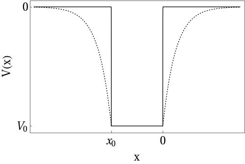
Figure 1: Smooth potential well for $V_{0}=2$ with $a=0.5$ (dotted line) and square potential well for $a=0.001$ (solid line).

4 Bound State Solutions

4.1 Bound state solutions for $x<x_{0}$

The bound state solutions for $x<x_{0}$ are obtained by solving the differential equation

$$\frac{\mathrm{d}^{2}\phi_{\textnormal{I}}(x)}{\mathrm{d}x^{2}}+\left\{\left[E+V_{0}e^{\frac{(x-x_{0})}{a}}\right]^{2}-1\right\}\phi_{\textnormal{I}}(x)=0.$$ (10)

On making the change of variable $y=2iaV_{0}e^{\frac{(x-x_{0})}{a}}$, Eq. (10) becomes

$$y\frac{\mathrm{d}}{\mathrm{d}y}\left(y\frac{\phi_{\textnormal{I}}}{\mathrm{d}y}\right)-\left[\left(iaE+\frac{y}{2}\right)^{2}+a^{2}\right]\phi_{\textnormal{I}}=0.$$ (11)

Putting $\phi_{\textnormal{I}}=y^{-\nicefrac{{1}}{{2}}}f(y)$ we obtain the Whittaker differential equation

$$f(y)^{\prime\prime}+\left[-\frac{1}{4}\textasciiacute-\frac{iaE}{y}+\frac{\nicefrac{{1}}{{4}}-a^{2}(1-E^{2})}{y^{2}}\right]f(y)=0,$$ (12)

which general solution is given by

$$f(y)=c_{1}M_{\kappa,\mu}(y)+d_{1}W_{\kappa,\mu}(y),$$ (13)

where $M_{\kappa,\mu}(y)$, $W_{\kappa,\mu}(y)$ are the Whittaker functions, $\kappa=-iaE$, and $\mu=a\sqrt{1-E^{2}}$. Then the solution of Eq. (11) is given by,

$$\phi_{\textnormal{I}}(y)=b_{1}y^{-\nicefrac{{1}}{{2}}}M_{\kappa,\mu}(y)+b_{2}y^{-\nicefrac{{1}}{{2}}}W_{\kappa,\mu}(y).$$ (14)

Since we are looking for bounds states of equation (10), we choose to work with regular solutions of $\phi_{\textnormal{I}}$ along the $x$ axis. If $x\rightarrow-\infty,\quad y\rightarrow 0$, the limits of the Whittaker functions are given by

$$\lim\limits_{y\rightarrow 0}\,y^{-\nicefrac{{1}}{{2}}}M_{\kappa,\mu}(y) \rightarrow 0,$$ (15)

$$\lim\limits_{y\rightarrow 0}\,y^{-\nicefrac{{1}}{{2}}}W_{\kappa,\mu}(y) \rightarrow \textnormal{complex infinity}.$$ (16)

Then the regular solution is,

$$\phi_{\textnormal{I}}(x)=b_{1}(2iaV_{0})^{-\nicefrac{{1}}{{2}}}e^{-\frac{(x-x_{0})}{2a}}M_{\kappa,\mu}\left[2iaV_{0}e^{\frac{(x-x_{0})}{a}}\right].$$ (17)

4.2 Bound state solutions for $x_{0}\leq x\leq 0$

The bound solutions for $x_{0}<x<0$ are obtained by solving the differential equation

$$\frac{\mathrm{d}^{2}\phi_{\textnormal{II}}(x)}{\mathrm{d}x^{2}}+\left[\left(E+V_{0}\right)^{2}-1\right]\phi_{\textnormal{II}}(x)=0.$$ (18)

Eq. (18) has the general solution

$$\phi_{\textnormal{II}}(x)=b_{3}\,e^{-iqx}+b_{4}\,e^{iqx},$$ (19)

where $q=\sqrt{\left(E+V_{0}\right)^{2}-1}$.

4.3 Bound state solutions for $x>0$

The scattering solutions for $x>0$ are obtained by solving the differential equation

$$\frac{\mathrm{d}^{2}\phi_{\textnormal{III}}(x)}{\mathrm{d}x^{2}}+\left[\left(E+V_{0}e^{-\frac{x}{a}}\right)^{2}-1\right]\phi_{\textnormal{III}}(x)=0.$$ (20)

On making the change of variable $z=2iaV_{0}e^{-\frac{x}{a}}$, Eq. (20) becomes

$$z\frac{\mathrm{d}}{\mathrm{d}z}\left(z\frac{\phi_{\textnormal{III}}}{\mathrm{d}z}\right)-\left[\left(iaE+\frac{z}{2}\right)^{2}+a^{2}\right]\phi_{\textnormal{III}}=0.$$ (21)

Putting $\phi_{\textnormal{III}}=z^{-\nicefrac{{1}}{{2}}}g(z)$ we obtain the Whittaker differential equation

$$g(z)^{\prime\prime}+\left[-\frac{1}{4}-\frac{iaE}{z}+\frac{\nicefrac{{1}}{{4}}-a^{2}(1-E^{2})}{z^{2}}\right]g(z)=0,$$ (22)

which solution is given by

$$g(z)=b_{5}M_{\kappa,\mu}(z)+b_{6}W_{\kappa,\mu}(z).$$ (23)

The solution of Eq. (21) becomes

$$\phi_{\textnormal{III}}(z)=b_{5}z^{-\nicefrac{{1}}{{2}}}M_{\kappa,\mu}(z)+b_{6}z^{-\nicefrac{{1}}{{2}}}W_{\kappa,\mu}(z).$$ (24)

Searching the regular solution: if $x\rightarrow\infty,\quad y\rightarrow 0$, the limits of the Whittaker functions are given by

$$\lim\limits_{z\rightarrow 0}\,z^{-\nicefrac{{1}}{{2}}}M_{\kappa,\mu}(z) \rightarrow 0,$$ (25)

$$\lim\limits_{z\rightarrow 0}\,z^{-\nicefrac{{1}}{{2}}}W_{\kappa,\mu}(z) \rightarrow \textnormal{complex infinity}.$$ (26)

Then, in terms of the variable $x$, the regular solution becomes

$$\phi_{\textnormal{III}}(x)=b_{5}\,(2iaV_{0})^{(-\nicefrac{{1}}{{2}})}e^{\frac{x}{2a}}M_{\kappa,\mu}\left(2iaV_{0}e^{-\frac{x}{a}}\right).$$ (27)

5 Results and discussion

In order to find bound states, we impose the condition that the wave functions and their first derivatives must be continuous at $x=x_{0}$ and $x=0$. Working algebraically with the resulting system of equations we obtain that the energy eigenvalues must satisfy the equation

$$\dfrac{1}{4a^{2}}\left\{\left[1+2\kappa+2ia(q-V_{0})\right]M_{\kappa,\mu}(2iaV_{0})-(1+2\kappa+2\mu)M_{1+\kappa,\mu}(2iaV_{0})^{2}\right\}^{2}$$

$$- \dfrac{e^{-2ix_{0}q}}{4a^{2}}\left\{\left[1+2\kappa-2ia(q+V_{0})\right]M_{\kappa,\mu}(2iaV_{0})-(1+2\kappa+2\mu)M_{1+\kappa,\mu}(2iaV_{0})\right\}^{2}=0.$$

The explicit solutions of Eq. (5), showing the dependence of the energy $E$ on $V_{0}$, $a$ and $x_{0}$ can be determined numerically. Fig (2) shows the dependence of the spectrum of bound states on the potential strength $V_{0}$, for $2.715<V_{0}\leq 2.735$ two states appear, one with positive energy and another with negative energy. The bound antiparticle state joins with the bound particle state at $V_{\textnormal{cr}}=2.7322$ where they form a state with zero norm.

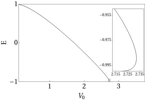
Figure 2: Bound-state spectrum for $a=0.5$ and $x_{0}=-0.5$.

The normalization of the wave functions (17), (19), and (27), with the respective value of $b_{1}$, $b_{3}{\tiny}$, and $b_{5}$ in terms of $b_{4}$ obtained from the continuity conditions, is given by

$$N=2\int^{\infty}_{-\infty}dx[E-V(x)]\phi(x)^{*}\phi(x).$$ (29)

The norm of the Klein-Gordon equation vanishes at $V_{cr}$, where both possible solution $E^{(+)}$ and $E^{(-)}$ meet. Particle bound states ($E^{(+)}$) and antiparticle bound states ($E^{(-)}$) correspond to $N>0$ and $N<0$ respectively. For $N=0$ both solutions meet and have the same energy. In Fig. 2 the antiparticle bound state appears at $V_{0}=2.72$, and the norm of two points before reaching $V_{\textnormal{cr}}$ is showing in Table 1.

$E$	$V_{0}$	$N$	Comment
- 0.979087	2.73	4.16463	Particle bound state
- 0.996487	2.73	- 8.08205	Antiparticle bound state

Table 1: Value of the norm for two points of the curve showed in Fig. 2.

Antiparticle bound states appear in all cases considered. For $a=0.5$, we moved the width parameter $x_{0}$ from $0$ to $-5$. Fig 3 shows the bound-state spectrum for $a=0.5$ and three different values of $x_{0}$, we can observed that the value of $V_{\textnormal{cr}}$ decreases as $\left|x_{0}\right|$ increases. Note that for $x_{0}=0$ we recover the results for the cusp potential well [5], also if we consider $x_{0}\neq 0$ and $a\rightarrow 0$ we recover the result for the square potential well [25].

Fig. 4 shows the behavior of the energy $E$ versus the potential parameter $x_{0}$. We can observe that as the value of $\left|x_{0}\right|$ increases, the energy value, for which antiparticle states appears, decreases.

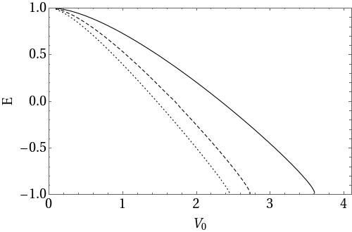
Figure 3: Bound-state spectrum for $a=0.5$ and three different values of $x_{0}$. Solid line represents $x_{0}=0$, dashed-line represents $x_{0}=-0.5$, and dotted line represents $x_{0}=-1$.

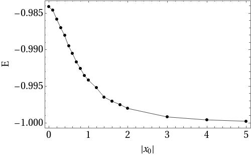
Figure 4: Energy vs width of the smooth potential well for $a=0.5$.

6 Conclusions

In this paper we have studied the bound state solutions of the Klein-Gordon equation in presence of a smooth potential well. We have calculated the energy eigenvalues as function of the parameters of the potential, and the antiparticle bound state appears in all cases considered. For certain values of the smoothness and width of the smooth potential well we recover the results of the cusp potential well [5] and the square potential well [25].

References

- [1] J. Rafelski, L. P. Fulcher, and A. Klein. Fermions and bosons interacting with arbitrarily strong external fields. Phys. Rep., 38:227, 1978.
- [2] Schiff, L. I., Snyder, H. and Weinberg, J. On the existence of stationary states of the mesotron field. Phys. Rev., 57:315, 1940.
- [3] M. Bawin. Klein-Gordon Particles in Deep Square Wells. Lett. Nuovo Cimento, 26:586, 1979.
- [4] C. Rojas and V. M. Villalba. The Klein-Gordon equation with the Woods-Saxon potential well. Rev. Mex. Fis, 52:127, 2006.
- [5] V. M. Villalba and C. Rojas. Bound states of the Klein-Gordon equation in the presence of short range potentials. Int. J. Mod. Phys. A, 21:313, 2006.
- [6] O. Aydodu, A. Arda, and R. Server. Effective-mass Dirac equation for Woods-Saxon potential: Scattering, bound states, and resonances. J. Math Phys, 53:042106, 2012.
- [7] G. Chen, Z.-D. Chena and Z.-M. Loua. Exact bound state solutions of the s-wave Klein-Gordon equation with the generalized Hulthén potential. Phys. Lett. A, 367:498, 2007.
- [8] H. Hassanabadi, S. Zarrinkamar and E. Maghsoodi. Cusp interation in minimal length quantum mechanics. Body Syst., 55:255, 2014.
- [9] Wen-Du Li and Wu-Sheng Dai. Exact solution of inversesquareroot potential . Ann. Phys., 373:207, 2016.
- [10] B. C. Lütfüogl, F. Akdeniz, and O. Bayrak. Scattering, bound, and quasi-bound states of the generalized symmetric Woods-Saxon potential. J. Math Phys, 57:032103, 2016.
- [11] C. Rojas and V. M. Villalba. Scattering of a Klein-Gordon particle by a Woods-Saxon potential. Phys. Rev. A, 71:052101, 2005.
- [12] V. M. Villalba and C. Rojas. Scattering of a relativistic scalar particle by a cusp potential. Phys. Lett. A, 362:21, 2007.
- [13] V. M. Villalba and L. A. GonzálezDíaz. Resonant states in an attractive one-dimensional cusp potential. Phys. Scr., 75:645, 2007.
- [14] C. Rojas. Scattering of a relativistic particle by a hyperbolic tangent potential. Can. J. Phys., 99:1, 2014.
- [15] C. Rojas. Scattering solutions of the kleingordon equation for a step potential with hyperbolic tangent potential. Mod. Phys. Lett. A, 29:1450146, 2014.
- [16] A. N. Ikok, H. Hassanabadi, N. Salehi, H. P. Obong and M. C. Onyeaju. Scattering states of cusp potential in minimal length dirac equation. Indian J. Phys, 89:1221, 2015.
- [17] M. Chabab, A. El Batoul, H. Hassanabadi, M. Oulne and S. Zare. Scattering states of dirac particle equation with position-dependent mass under the cusp potential. Eur. Phys. J. Plus, 131:2016, 2016.
- [18] B. C. Lütfüogl, A. N. Ikot, E. O. Chukwocha, and F. E. Bazuaye. Analytical solution of the Klein Gordon equation with a multi-parameter q-deformed Woods-Saxon type potential. Eur. Phys. J. Plus, 133, 2018.
- [19] E. J. Aquino Curi, L. B. Castro and A. S. de Castro. Proper treatment of scalar and vector exponential potentials in the klein-gorodon equations: Scattering and bound states. Eur. Phys. J. Plus, 134:248, 2019.
- [20] E. López and C. Rojas. Scattering of a klein-gordon particle by a smooth barrier. Can. J. Phys, In press, 2020.
- [21] M. Bawin and J. P. Lavine. The exponential potential and the klein-gordon equaion. IL Nuo. Cim. A, 23:311, 1974.
- [22] C. A. Manogue. The Klein paradox and superradiance. Ann. Phys, 181:261, 1988.
- [23] A. Molgado, O. Morales and J. A. Vallejo. Virtual beams and the klein paradox for the klein-gordon equation. Rev. Mex. Fis. E, 64:1, 2018.
- [24] L. Puentes, C. Cocha and C. Rojas. Study of superradiance in the lambert-w potential barrier. Int. J. Mod. Phys. A, 34:1950087, 2019.
- [25] W. Greiner. Relativistic Quantum Mechanics. Wave equations. Springer, 1987.