A comparison between quantum and classical noise radar sources

Abstract

We compare the performance of a quantum radar based on two-mode squeezed states with a classical radar system based on correlated thermal noise. With a constraint of equal number of photons $N_{S}$ transmitted to probe the environment, we find that the quantum setup exhibits an advantage with respect to its classical counterpart of $\sqrt{2}$ in the cross-mode correlations. Amplification of the signal and the idler is considered at different stages of the protocol, showing that no quantum advantage is achievable when a large-enough gain is applied, even when quantum-limited amplifiers are available. We also characterize the minimal type-II error probability decay, given a constraint on the type-I error probability, and find that the optimal decay rate of the type-II error probability in the quantum setup is $\ln(1+1/N_{S})$ larger than the optimal classical setup, in the $N_{S}\ll 1$ regime. In addition, we consider the Receiver Operating Characteristic (ROC) curves for the scenario when the idler and the received signal are measured separately, showing that no quantum advantage is present in this case. Our work characterizes the trade-off between quantum correlations and noise in quantum radar systems.

I Introduction

The quantum Illumination (QI) protocol [1, 2, 3, 4, 5, 6, 7] uses entanglement as a resource to improve the detection of a low-reflectivity object embedded in a bright environment. The protocol was first developed for a single photon source [1], and it was then extended to general bosonic quantum states and thermal bosonic channels [2]. Here, a $6$ dB advantage in the effective signal-to-noise ratio (SNR) is achievable when using two-mode squeezed states instead of coherent states. This gain has been recently shown to be optimal, and reachable exclusively in the regime of low transmitting power per mode [8, 9]. The QI protocol has possible applications in the spectrum below the Terahertz band, as here the environmental noise is naturally bright. In particular, microwave quantum technology has been very well developed in the last decades [10], paving the way of implementing these ideas for building a first prototype of quantum radar.

The possible benefits of a quantum radar system are generally understood to be situational. In an adversarial scenario, it is beneficial for a radar system to be able to operate while minimizing the power output, in order to reduce the probability for the transmitted signals to be detected. This property is commonly referred to as Low Probability of Intercept (LPI), and it is a common measure to limit the ability of the enemy to localize and discover the radar. The low signal levels required for QI are in principle excellent for acquiring good LPI properties. However, there are several challenges to face in order to achieve this goal. A first proposal for implementing a microwave QI protocol was advanced in Ref. [11]. The protocol relies on an efficient microwave-optical interface for the idler storage and the measurement stage. This technology is promising for this and other applications, however it is still in its infancy. Furthermore, the signal generation requires cryogenic technology, which must be interfaced with a room-temperature environment. Recently, a number of QI-related experiments have been carried out in the microwave regime [12, 13], showing that some correlations of an entangled signal-idler system are preserved after the signal is sent out of the dilution refrigerator. While these results are a good benchmark for future QI experiments, they strictly rely on the amplification of the signal and idler. This has been shown to rule out any quantum advantage with respect to an optimal classical reference [14].

In this work, we discuss the role of quantum correlations and amplification in the QI protocol, providing a comparative analysis of quantum and classical noise radars in different scenarios. Noise radar is an old concept that operates by probing the environment with a noisy signal and cross-correlating the returns with a retained copy of the transmitted signal [15]. A quantum noise radar operates similarly to its conventional counterpart, but differs in the use of a two-mode entangled state as noise source [12, 13]. An advantage of the quantum noise radar over the classical counterpart can be declared if stronger correlations can be achieved, when both systems illuminate the environment with equal power. In the microwave regime, the two-mode squeezed state used for noise correlations can be generated with superconducting circuits with a Josephson Parametric Amplifier (JPA) at $T\simeq 20$ mK [16, 17]. On the one hand, using quantum correlated signals generated by a JPA enhances the signal-to-noise ratio in the low transmitting power per mode regime. On the other hand, Josephson parametric circuits are able to generate correlated and entangled signals with large bandwidth [18, 19, 20]. This allows, in principle, a system to operate in the low power-per-mode regime, where quantum radars show fully their advantage. Here, we analyze the performance of a JPA-based noise radar in different scenarios which include different sources of noise. Our analysis shows that any quantum advantage is destroyed by the unavoidable noise added when amplifying either the signal or the idler. We also show when the idler and signal are measured separately, the entanglement initially present in the signal-idler system is not properly exploited, and no quantum advantage can be retained. The latter happens even without amplifying the signal or the idler. Our work complements the analysis done in Ref. [14] with the explicit calculations of the cross-correlation coefficients and the optimal asymptotic ROC performance in the microwave regime.

II Theory

In this section, we introduce the models for the quantum and classical systems, within the quantum mechanical description. In this step, we emulate Refs. [21, 14], where the classical and quantum noise radar were first studied. In all expressions, we assume the natural units ($\hbar=1$, $k_{\text{B}}=1$).

II-A Quantum preliminaries

A single, narrowband mode of the electric field, at microwave frequency $f$, is defined with an operator (in suitable units) as $\hat{E}=\hat{q}\cos{2\pi ft}+\hat{p}\sin{2\pi ft},$ where $\hat{q}$ and $\hat{p}$ are the in-phase and quadrature operators, respectively. The quadratures are related to the bosonic annihilation ($\hat{a}$) and creation ($\hat{a}^{\dagger}$) operators as $\hat{q}=(\hat{a}^{\dagger}{+}\hat{a})/\sqrt{2}$ and $\hat{p}=\mathrm{i}(\hat{a}^{\dagger}{-}\hat{a})/\sqrt{2}$, where $[\hat{a},\hat{a}^{\dagger}]=\hat{\mathbb{I}}$. The commutation relation $[\hat{q},\hat{p}]=\mathrm{i}\hat{\mathbb{I}}$ implies that the quadratures can not be measured simultaneously with arbitrary precision, due to the Heisenberg uncertainty relation. In the following, we represent the quadratures of the two-modes of the electric field by the vector $\hat{X}=(\hat{q}_{S},\hat{p}_{S},\hat{q}_{I},\hat{p}_{I})^{T}$, where the indices $S$ and $I$ refer to the signal and idler mode, respectively. These mode designations are used interchangeably for both the quantum and classical system.

II-A1 Classically-correlated thermal noise

Figure 1: Preparation of classically-correlated thermal noise. A beamsplitter with reflection coefficient $\xi$ and phase turning angle $\varphi$ generates the signal and idler modes from the modes $\hat{a}_{0}$ and $\hat{a}_{1}$. These modes are in a thermal state with $T_{0}$ and $T_{1}$ effective noise temperatures, respectively. The output modes are correlated provided that $T_{0}\not=T_{1}$.

The classically-correlated noise (CCN) system uses two sources of thermal noise, $\hat{a}_{0}$ and $\hat{a}_{1}$, at temperatures $T_{0}$ and $T_{1}$, respectively. In general, the quantum state of a thermal noise mode at temperature $T$ can be represented by the density operator

$$\mathbf{{\rho}}_{th}=\sum_{n=0}^{\infty}\frac{N^{n}}{\left(N+1\right)^{n+1}}\ket{n}\bra{n},$$ (1)

where the average number of photons is defined by the thermal equilibrium Bose-Einstein statistics at temperature $T$, i.e., $N=\left[\exp\left(2\pi f/T\right)-1\right]^{-1}$. In the following, we will refer as $N_{0}$ ($N_{1}$) the average number of photons for the mode $\hat{a}_{0}$ ($\hat{a}_{1}$). The thermal modes $\hat{a}_{0}$ and $\hat{a}_{1}$ pass through a beamsplitter, as shown in Fig. 1. This generates a signal mode $\hat{a}_{S}^{(C)}$ and an idler mode $\hat{a}_{I}^{(C)}$, related to the inputs as [22]

$$\begin{pmatrix}\hat{a}_{S}^{(C)}\\ \hat{a}_{I}^{(C)}\end{pmatrix}=\begin{pmatrix}\sqrt{\xi}&\sqrt{1-\xi}\mathrm{e}^{\mathrm{i}\varphi}\\ -\sqrt{1-\xi}\mathrm{e}^{-\mathrm{i}\varphi}&\sqrt{\xi}\end{pmatrix}\begin{pmatrix}\hat{a}_{0}\\ \hat{a}_{1}\end{pmatrix}.$$ (2)

Here, $\xi\in(0,1)$ is the reflection coefficient and $\varphi$ is the phase turning angle of the beamsplitter, in the following set to be zero. One can think of this process as a noise signal, generated by a thermal source at temperature $T_{0}$, sent as input of a power divider placed in an environment at temperature $T_{1}$. The output modes $\hat{a}_{S}^{(C)}$ and $\hat{a}_{I}^{(C)}$ are in a thermal state with $\xi N_{0}+(1-\xi)N_{1}$ and $\xi N_{1}+(1-\xi)N_{0}$ average number of photons, respectively. If $T_{1}\not=T_{0}$, or, equivalently, $N_{1}\not=N_{0}$, then the outputs are classically-correlated, regardless of the value of $\xi$.

II-A2 Entangled thermal noise

A Two-Mode Squeezed Vacuum (TMSV) state $\ket{\psi}_{\rm TMSV}$ is represented in the Fock basis as

$$\ket{\psi}_{\rm TMSV}=\sum_{n=0}^{\infty}\sqrt{\frac{N_{S}^{n}}{\left(N_{S}+1\right)^{n+1}}}\ket{n}_{S}\ket{n}_{I},$$ (3)

where $N_{S}$ is the average number of photons in both the signal and idler mode. A TMSV state is closely related to a classically-correlated thermal noise, as also here both signal and idler photons are Bose-Einstein distributed. However, as we will see, the resulting correlations in the low signal-power regime are stronger for the TSMV states.

II-B Covariance and correlation matrices

As the states considered here are Gaussian, their statistics is entirely determined by the first and second order quadrature moments. For zero-mean states, i.e., when $\braket{\hat{X}_{i}}=0$ for all $i$, the states are characterized entirely by the covariance matrix $\mathbf{\Sigma}$, with elements

$$\mathbf{\Sigma}_{i,j}=\frac{1}{2}\braket{\hat{X}_{i}\hat{X}_{j}^{\dagger}+\hat{X}_{j}\hat{X}_{i}^{\dagger}}-\braket{\hat{X}_{i}}\braket{\hat{X}_{j}^{\dagger}}.$$ (4)

This is the case for both the classical and the entangled thermal noise states. Similarly, one can introduce the correlation coefficient matrix $\mathbf{R}$, whose elements are

$$\mathbf{R}_{i,j}=\frac{\Sigma_{i,j}}{\sqrt{\Sigma_{i,i}}\sqrt{\Sigma_{j,j}}}\in[-1,1].$$ (5)

These coefficients, also referred to as Pearson’s correlation coefficients, characterize the linear dependence between the quadratures $\hat{X}_{i}$ and $\hat{X}_{j}$.

II-C Quantum relative entropy

The quantum relative entropy defines an information measure between two quantum states. It is defined as

$$D(\rho_{1}||\rho_{0})=\text{Tr}\,\rho_{1}(\ln\rho_{1}-\ln\rho_{0}),$$ (6)

for two density matrices $\rho_{0}$ and $\rho_{1}$. This quantity is related to the performance in the asymmetric binary hypothesis testing via the quantum Stein’s lemma. The task is to discriminate between $M$ copies of $\rho_{0}$ and $M$ copies of $\rho_{1}$, given a bound on the type-I error probability (probability of false alarm, $P_{Fa}$) of $\varepsilon\in(0,1)$. In this discrimination, the maximum type-II error probability (probability of miss, $P_{M}$) exponent is

$$\small-\frac{\ln P_{M}}{M}=D(\rho_{1}||\rho_{0})+\sqrt{\frac{V(\rho_{1}||\rho_{0})}{M}}\Phi^{-1}(\varepsilon)+\mathcal{O}\left(\frac{\ln M}{M}\right),$$ (7)

where $V(\rho_{1}||\rho_{0})=\text{Tr}\,\rho_{1}[\ln\rho_{1}-\ln\rho_{0}-D(\rho_{1}||\rho_{0})]^{2}$ is the quantum relative entropy variance and $\Phi^{-1}$ is the inverse cumulative normal distribution [23]. In this work, we rely on quantum relative entropy computations and its variance in order to quantify the performance in the asymptotic setting, i.e., when $M\gg 1$. This is in contrast to the original treatment based on the Chernoff bound [2], which provides an estimation of the average error probability when the prior probabilities of target absence or presence are equal. In a typical radar scenario, the prior probabilities are not the same, and may be even unknown.

III Noise radar operation

In this section, we analyze the performance of the classical and quantum noise correlated radars, based on the states defined in the previous section.

III-A Probing the environment

The signal mode is transmitted to probe the environment where an object (target) may be present or absent. This process is modelled as a channel with reflection coefficient $\eta$ that is non-zero and small when the target is present ($0<\eta\ll 1$) and zero when the target is absent ($\eta=0$), see Fig. 2. Here, $\eta$ can be interpreted as the ratio between transmitted power and received power, including the effects of atmospheric attenuation, the antenna gain and the target radar cross section. We use a beamsplitter model to take into account the environmental losses. In other words, the returned mode $\hat{a}_{R}$ is given by

$$\hat{a}_{R}=\sqrt{\eta}~{}\hat{a}_{S}\mathrm{e}^{-\mathrm{i}\theta}+\sqrt{1-\eta}~{}\hat{a}_{B},$$ (8)

where $\hat{a}_{B}$ is a bright background noise mode with $\braket{\hat{a}_{B}^{\dagger}\hat{a}_{B}}=N_{B}$ average power per mode, and where $\theta$ is a phase shift relative to the idler. In the $1-10$ GHz regime, where the technology is advanced enough to apply these ideas in the quantum regime, we have that $N_{B}\simeq 10^{3}$, which is assumed for numerical computations. For the current calculation, the reflection coefficient is assumed to be non-fluctuating. We also assume $\braket{\hat{a}_{I}\hat{a}_{B}}=0$, i.e., the returned signal preserves some correlations with the idler mode only if the object is present. This allows us to define a correlation detector able to detect the presence or absence of the object.

Figure 2: Scheme of the quantum and classical noise radar systems. The system probes a region of space with a signal $\hat{a}_{S}$ to detect a possible object, modelled as a channel with reflectivity parameter $\eta$. The returned signal $\hat{a}_{R}$ is then used for detecting correlations with the idler mode $\hat{a}_{I}$, which has been retained in the lab.

III-B Cross-correlation coefficient

The covariance matrix of the system composed of the received signal and the idler is easily computable using Eq. (4) and Eq. (8). For both the classical and the quantum noise radars considered here, applying Eq. (5) gives us the correlation matrix

$$\mathbf{R}=\begin{pmatrix}\mathbf{I}&\kappa\mathbf{D}(\theta)\\ \kappa\mathbf{D}(\theta)^{T}&\mathbf{I}\end{pmatrix},$$ (9)

where $0\leq\kappa\leq 1$ is the amplitude of the cross-correlation coefficient, and $\mathbf{D}$ is a matrix with determinant $\left|\mathbf{D}\right|=\pm 1$. The cross-correlation coefficient for the entangled TMSV source can be derived directly from the definition,

$$\kappa_{\text{TMSV}} =\frac{\sqrt{\eta N_{S}(N_{S}+1)}}{\sqrt{N_{R}+\frac{1}{2}}\sqrt{N_{S}+\frac{1}{2}}},$$ (10)

with $N_{R}=\eta N_{S}+(1-\eta)N_{B}$. For a fair comparison between the quantum and classical systems, we introduce a constraint on the transmitted power of the signal modes, i.e., we set

$$N_{S}=\xi N_{0}+(1-\xi)N_{1}.$$ (11)

This constraint can be interpreted as giving both systems equal LPI properties. Eq. (11) yields an expression for the classical cross-correlation amplitude as

$$\kappa_{\text{CCN}}=\frac{\sqrt{\eta}(N_{S}-N_{1})}{\sqrt{N_{R}+\frac{1}{2}}\sqrt{N_{S}-N_{1}+\frac{\xi}{1-\xi}\left(N_{1}+\frac{1}{2}\right)}},$$ (12)

where $N_{S}>N_{1}$ follows directly from Eq. (11) and the assumption $N_{0}>N_{1}$. This quantity is maximal in the $N_{1}\ll 1$ regime, where Eq. (11) reduces to $N_{S}=\xi N_{0}$. We assume $N_{1}\ll 1$, which corresponds to classically-correlated thermal noise generated in a noise-free environment. At microwave frequencies this is achievable at mK temperatures. Eq. (12), for given noise transmitting power, defines the correlations of a class of classical noise radars, labeled by the beamsplitter parameter $\xi$.

III-C Quantum advantage

It is easy to see that the quantity $\kappa^{2}$ is linearly proportional to the effective SNR in the likelihood-ratio tests. A larger value of $\kappa^{2}$ means a stronger discrimination power. Therefore, we define a figure of merit $Q_{A}$, quantifying the advantage of the quantum over the classical noise radar, as

$$Q_{A} \equiv\frac{\kappa_{\text{TMSV}}^{2}}{\kappa_{\text{CCN}}^{2}}=\frac{N_{S}+1}{N_{S}+\frac{1}{2}}\left[1+\frac{\xi}{2N_{S}(1-\xi)}\right],$$ (13)

which can be evaluated for different values of the free parameter $\xi$. Restricting the constraint to equal power in both the signal and idler mode is equivalent to applying a 50-50 beamsplitter to the thermal noise source in Eq. (2), or, in other words, it corresponds to setting $\xi~{}=~{}1/2$. This gives

$$Q_{A}(\xi=1/2)=1+\frac{1}{N_{S}},$$ (14)

which is unbounded for $N_{S}\rightarrow 0$. This setting as been used as benchmarking in the recent microwave quantum illumination experiments [12, 13]. However, this choice of $\xi$ is not optimal, leading to an overestimation of the quantum radar advantage. A strongly asymmetric beamsplitter must be applied to a very bright noise source ($N_{0}\gg 1$) in order to maximize the correlations in the classical case, while maintaining the constraint on transmitted power $N_{S}=\xi N_{0}$. It can be seen in Eq. (13), that $Q_{A}$ is maximized in the $\xi/(1-\xi)\ll N_{S}$ limit. In this setting, the CCN idler has a much better SNR than in the symmetric configuration, and we get

$$Q_{A}(\xi/(1-\xi)\ll N_{S})\approx 2\left[1-\frac{N_{S}}{2N_{S}+1}\right].$$ (15)

In the low transmitting power limit we have that $\lim\limits_{N_{S}\rightarrow 0}Q_{A}=2$, i.e., a $\sqrt{2}$ advantage in the correlation coefficient. In Fig. 3 we show the functional behaviour of the correlation coefficients for the entangled and classically-correlated thermal noise source, depending on the transmitting power $N_{S}$. The quantum advantage decays slowly with increasing $N_{S}$, keeping an advantage also for finite $N_{S}$, until virtually disappearing for $N_{S}\simeq 10$. Note that in the limit where the advantage is maximized, the modes also become uncorrelated ($\kappa\rightarrow 0$) in both systems. A signal-idler system with a large operating bandwidth is needed to compensate the low amount of correlations per mode in the $N_{S}\ll 1$ limit.

Here, the phase-shift of the signal mode due to the propagating path has been set to zero. In other words, we work in a rotated frame, where the inter-mode phase angle $\theta$ is applied only to the idler mode, i.e., $\hat{a}_{I}\mapsto\hat{a}_{I}\mathrm{e}^{-\mathrm{i}\theta}$. Note that, in general, the phase $\theta$ is unknown. The original QI protocol assumes the knowledge of the inter-mode phase angle $\theta$. In this case, the complex conjugate receiver defined in Ref. [24] saturates the quantum advantage given in Eq. (13) with a likelihood-ratio test [25]. If $\theta$ is unknown, then one can define an adaptive strategy where $\mathcal{O}(\sqrt{M})$ copies are used to get a rough estimate of $\theta$, and then $M-\mathcal{O}(\sqrt{M})$ are used to perform the discrimination protocol in the optimal reference frame maximizing the Fisher information [7]. This strategy shows the same asymptotic performance as in the case of known $\theta$.

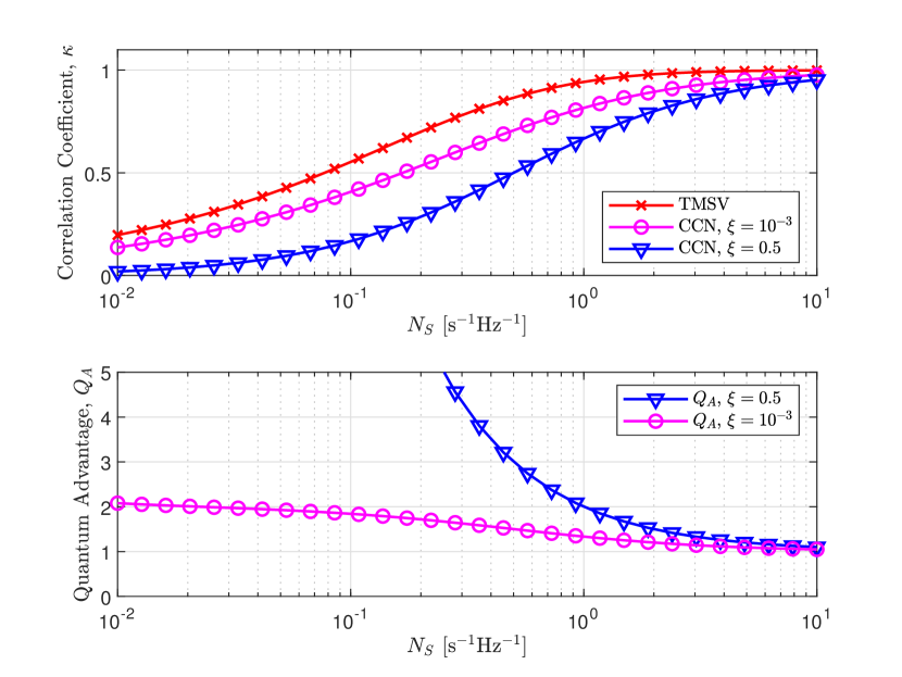
Figure 3: Performance of the quantum and classical noise radars in terms of the cross-correlation coefficient. (Upper) The cross-correlation coefficients for the quantum and classical noise radars, as functions of the transmitted quanta, rescaled such that $\sqrt{\eta}=1$. (Lower) The quantum advantage for the cases considered above. In both plots, we have considered the $\xi=10^{-3}$ and $\xi=0.5$ settings. The first setting achieves a close to optimal cross-correlation coefficient. The second setting is suboptimal, and it has been used as classical reference in recent microwave illumination experiments [12, 13].

III-D The effect of amplification

In the following, we consider three Gaussian amplifying schemes. We show how the quantum advantage defined in terms the cross-correlation coefficients rapidly disappears when an amplification is involved at any stage of the protocol.

III-D1 Amplification before transmitting the signal mode

If we amplify the signal mode before transmission to the environment, the transmitted mode is $\hat{a}_{S}^{\prime}=\sqrt{G_{S}}~{}\hat{a}_{S}+\sqrt{G_{S}-1}~{}\hat{a}_{G_{S}}^{\dagger},$ where $G_{S}\geq 1$ is the gain and where $\braket{\hat{a}_{G_{S}}^{\dagger}\hat{a}_{G_{S}}}=N_{G_{S}}$ is the added noise. The classical and quantum covariance matrix transforms identically. Correspondingly, the advantage in Eq. (13) is actually independent of the signal amplification. However, although $G_{S}$ counteracts the loss due to $\eta$, the added noise limits the absolute correlations that can be achieved. In addition, in the weak signal regime where the quantum advantage is relevant, the effective SNR is low even before amplification. Amplifying a signal with low SNR is trivially outperformed by using a stronger signal with better SNR to begin with, as is the case of a classically-correlated thermal noise with $G_{S}N_{S}+(G_{S}-1)(N_{G_{S}}+1)$ average signal photons. In addition, any sufficiently strong amplification applied at this stage would weaken LPI properties, and possibly move the system to a regime where another protocol outperforms correlation detection.

III-D2 Amplification before measurement

These amplification schemes describe the pre-amplification of the modes in heterodyne quadratures measurement.

With $G_{R}\geq 1$ amplifying the returned mode, as $\hat{a}_{R}^{\prime}=\sqrt{G_{R}}~{}\hat{a}_{R}+\sqrt{G_{R}-1}~{}\hat{a}_{G_{R}}^{\dagger},$ the covariance matrix again transforms identically for the quantum and classical systems, and any added noise cancels in the advantage merit. However, as can be intuitively understood, amplification at the receiver end can not increase correlations with the idler reference. Indeed, the added amplifier noise reduces correlations, but equally in both systems.

Instead, applying the amplification $G_{I}\geq 1$ to the idler, as $\hat{a}_{I}^{\prime}=\sqrt{G_{I}}~{}\hat{a}_{I}+\sqrt{G_{I}-1}~{}\hat{a}_{G_{I}}^{\dagger},$ is actually detrimental to the advantage of Eq. (13). In the limit of strong amplification ($G_{I}\gg 1$), the advantage merit is

$$Q_{A}=\frac{N_{S}+1}{N_{S}+N_{G_{I}}+1}\left[1+\frac{\xi(N_{G_{I}}+1)}{N_{S}(1-\xi)}\right],$$ (16)

where $\braket{\hat{a}_{G_{I}}^{\dagger}\hat{a}_{G_{I}}}=N_{G_{I}}$ is the added noise. We consider the ideal case of quantum limited amplifier noise ($N_{G_{I}}\rightarrow 0$), which simplifies the quantum advantage to

$$Q_{A}=1+\frac{\xi}{N_{S}(1-\xi)}.$$ (17)

In this form it is clear that in the $\xi/(1-\xi)\ll N_{S}$ setting, all the quantum advantage is destroyed. Conversely, an unlimited quantum advantage can be observed in the $N_{S}\ll\xi$ regime.

III-E Receiver Operating Characteristic performance

In this section, we analyze the quantum and classical noise radar in the asymmetric setting, i.e., when the prior probabilities are not equal, under a different perspective. We derive the ROC curves in the case when the idler and the signal are separately measured with heterodyne detection. In addition, we show the asymptotic performances of the optimal quantum strategies.

III-E1 ROC curves with heterodyne detection

We assume measurement is performed with heterodyne detection of the four quadratures $\vec{X}=\braket{\hat{X}}$. Based on the observed data set $\mathbf{X}=\{\vec{X}_{1},\vec{X}_{2},\ldots,\vec{X}_{M}\}$, an optimal threshold detector is computed by maximizing the log-likelihood ratio test around $\eta\ll 1$. This detector has, by Wilks’s theorem, asymptotically Chi-squared statistical distribution. The ROC is computed in terms of the probability of detection ($P_{D}=1-P_{M}$) as

$$P_{D}=Q_{\chi_{1}^{\prime 2}(2M\kappa^{2})}\left(Q_{\chi_{1}^{2}}^{-1}(P_{Fa})\right),$$ (18)

where $Q$ is defined as the right-tail probability of the respective distribution. The performance for this detector is presented with an example in Fig. 4, for realistic parameters in the microwave regime. We see that the quantum source is not any better than a classical source, when $\xi/(1-\xi)\ll N_{S}$. This is due to the amount of noise added with heterodyne detection.

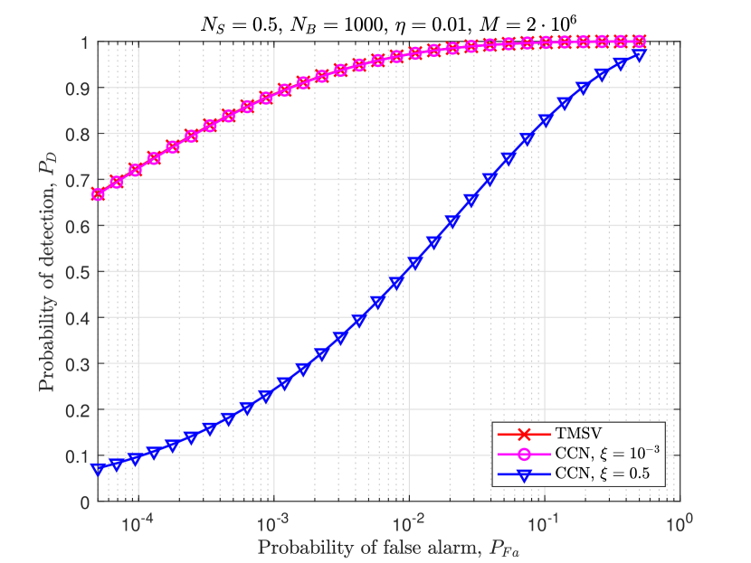
Figure 4: ROC curves with heterodyne detection for different radar systems. In the optimal classical setting, corresponding to $\xi/(1-\xi)\ll N_{S}$, the classical noise radar has the same ROC curve as the quantum noise radar. This shows how the entanglement initially present in the system is not properly exploited when the received signal and the idler are measured separately.

III-E2 Quantum Stein’s lemma

We provide the asymptotic performance as given in Subsection II-C. This analysis has been done for a radar system based on coherent state [23], but the classically-correlated noise case was missing. The quantum relative entropy rules the asymptotic behaviour of the error probability decay. These are given by

$$\small D_{\text{TMSV}}\simeq\frac{\eta N_{S}(N_{S}+1)}{N_{S}+N_{B}+1}\left[\ln\left(1+\tfrac{1}{N_{B}}\right)+\ln\left(1+\tfrac{1}{N_{S}}\right)\right],$$ (19)

$$\small D_{\text{CCN}}\simeq\frac{\eta N_{S}^{2}}{N_{S}-\tfrac{\xi N_{B}}{1-\xi}}\left[\ln\left(1{+}\tfrac{1}{N_{B}}\right){-}\ln\left(1{+}\tfrac{\xi}{N_{S}(1-\xi)}\right)\right],$$ (20)

to first order in $\eta$. One can easily see that the $\xi/(1-\xi)\ll N_{S}$ setting is optimal for the classical case. In particular, in the $N_{B}\gg 1\gg N_{S}\gg\xi$ regime, we have that $D_{\text{TMSV}}/D_{\text{CCN}}\sim\ln(1+1/N_{S})$. A substantial advantage can be also found for moderate values of $N_{S}$ (see Fig. 5). The variance of the quantum relative entropy provides the convergence rate of the error probability exponent to its asymptotic value, for the type-I error probability constrained to be lower than $\varepsilon$. We do not provide the explicit formula here. However, in Fig. 5 we depict an example for the values of $\xi$ previously considered, and for $\varepsilon=10^{-3}$.

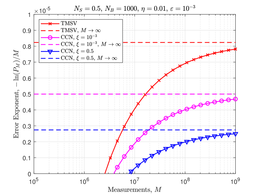
Figure 5: Asymptotic error probability exponent in the asymmetric setting. This is computed according to the quantum Stein’s lemma (see Eq. (7)). Here, we consider an optimal joint measurements of the idler and received signal for both the quantum and the classical radar systems. The amount of measurements $M$ needed for the error probability exponent to converge to the asymptotic values increases logarithmically in $\varepsilon^{-1}$, see Eq. (7). In the asymptotic regime, a $\ln(1+1/N_{S})$ advantage is achievable for $N_{S}\ll 1$, see Eqs. (19)-(20). However, a substantial advantage is achievable also for moderate values of $N_{S}$ (in the figure $N_{S}=0.5$).

IV Conclusion and Outlook

We have compared the performance of a quantum noise radar based on two-mode squeezed states and a class of noise radars based on thermal states. We have found that, given a constraint on the transmitting power, a quantum advantage in the ROC curve and their asymptotic performances is possible. If a low-powered signal of a quantum noise radar is amplified, then there is a classical noise radar which outperforms considerably the quantum radar. In addition, if enough noise is added at the idler level, such as when it is amplified or measured heterodyne, then all the quantum advantage is lost. However, a quantum advantage appears when the idler and signal are allowed to be measured jointly. Our results show that amplification is not a good strategy to overcome the technical difficulties that one must face in a practical quantum radar implementation. This suggests that quantum radars are more difficult to achieve than what recent experiments were claiming [13, 12]. Interfacing a large bandwidth entangled microwave signal with the environment, and developing low-noise power detectors is crucial for performing a QI experiment with a quantum advantage.

References

- [1] S. Lloyd, “Enhanced sensitivity of photodetection via quantum illumination,” Science, vol. 321, no. 5895, pp. 1463–1465, 2008.
- [2] S.-H. Tan et al., “Quantum illumination with gaussian states,” Physical Review Letters, vol. 101, no. 25, p. 253601, 2008.
- [3] E. D. Lopaeva, I. Ruo Berchera, I. P. Degiovanni, S. Olivares, G. Brida, and M. Genovese, “Experimental realization of quantum illumination,” Physical Review Letters, vol. 110, no. 15, p. 153603, 2013.
- [4] Z. Zhang, M. Tengner, T. Zhong, F. N. C. Wong, and J. H. Shapiro, “Entanglement’s benefit survives an entanglement-breaking channel,” Physical Review Letters, vol. 111, no. 1, p. 010501, 2013.
- [5] Z. Zhang, S. Mouradian, F. N. C. Wong, and J. H. Shapiro, “Entanglement-enhanced sensing in a lossy and noisy environment,” Physical Review Letters, vol. 114, no. 11, p. 110506, 2015.
- [6] Q. Zhuang, Z. Zhang, and J. H. Shapiro, “Optimum mixed-state discrimination for noisy entanglement-enhanced sensing,” Physical Review Letters, vol. 118, no. 4, p. 040801, 2017.
- [7] M. Sanz, U. Las Heras, J. J. Garcia-Ripoll, E. Solano, and R. Di Candia, “Quantum estimation methods for quantum illumination,” Physical Review Letters, vol. 118, no. 7, p. 070803, 2017.
- [8] R. Di Candia, H. Yiğitler, S. G. Paraoanu, and R. Jäntti, “Two-way covert microwave quantum communication,” arXiv:2004.07192, 2020.
- [9] R. Nair and M. Gu, “Fundamental limits of quantum illumination,” arXiv:2002.12252, 2020.
- [10] X. Gu, A. Frisk Kockum, A. Miranowicz, Y.-x. Liu, and F. Nori, “Microwave photonics with superconducting quantum circuits,” Physics Reports, vol. 718-719, pp. 1–102, 2017.
- [11] S. Barzanjeh, S. Guha, C. Weedbrook, D. Vitali, J. H. Shapiro, and S. Pirandola, “Microwave quantum illumination,” Physical Review Letters, vol. 114, no. 8, p. 080503, 2015.
- [12] C. S. Chang, A. Vadiraj, J. Bourassa, B. Balaji, and C. Wilson, “Quantum-enhanced noise radar,” Applied Physics Letters, vol. 114, no. 11, p. 112601, 2019.
- [13] S. Barzanjeh, S. Pirandola, D. Vitali, and J. Fink, “Microwave quantum illumination using a digital receiver,” Science Advances, vol. 6, no. 19, eabb0451, 2020.
- [14] J. H. Shapiro, “The quantum illumination story,” IEEE Aerosp. Electron. Sys. Mag., vol. 35, no. 4, p. 8–20, 2020.
- [15] G. R. Cooper et al., “Random signal radar,” ECE Technical Reports, 1967, Paper 366.
- [16] E. Flurin, N. Roch, F. Mallet, M. H. Devoret, and B. Huard, “Generating entangled microwave radiation over two transmission lines,” Physical Review Letters, vol. 109, no. 18, p. 183901, 2012.
- [17] E. P. Menzel et al., “Path entanglement of continuous-variable quantum microwaves,” Physical Review Letters, vol. 109, no. 25, p. 250502, 2012.
- [18] C. M. Wilson et al., “Observation of the dynamical casimir effect in a superconducting circuit,” Nature, vol. 479, pp. 376–379, 2011.
- [19] J. Johansson, G. Johansson, C. Wilson, P. Delsing, and F. Nori, “Nonclassical microwave radiation from the dynamical casimir effect,” Physical Review A, vol. 87, no. 4, p. 043804, 2013.
- [20] B. Schneider et al., “Observation of broadband entanglement in microwave radiation from a single time-varying boundary condition,” Physical Review Letters, vol. 124, no. 14, p. 140503, 2020.
- [21] D. Luong, C. Chang, A. Vadiraj, A. Damini, C. Wilson, and B. Balaji, “Receiver operating characteristics for a prototype quantum two-mode squeezing radar,” IEEE Transactions on Aerospace and Electronic Systems, vol. 56, no. 3, pp. 2041–2060, 2020.
- [22] R. Loudon, The quantum theory of light. OUP Oxford, 2000.
- [23] M. M. Wilde, M. Tomamichel, S. Lloyd, and M. Berta, “Gaussian hypothesis testing and quantum illumination,” Physical Review Letters, vol. 119, no. 12, p. 120501, 2017.
- [24] S. Guha and B. I. Erkmen, “Gaussian-state quantum-illumination receivers for target detection,” Physical Review A, vol. 80, no. 5, p. 052310, 2009.
- [25] Q. Zhuang, Z. Zhang, and J. H. Shapiro, “Entanglement-enhanced neyman-pearson target detection using quantum illumination,” Journal of the Optical Society of America B, vol. 34, no. 8, p. 1567, 2017.