Bandwidth Cost of Code Conversions in Distributed Storage: Fundamental Limits and Optimal Constructions

Abstract

Erasure codes have become an integral part of distributed storage systems as a tool for providing data reliability and durability under the constant threat of device failures. In such systems, an $[n,k]$ code over a finite field $\mathbb{F}_{q}$ encodes $k$ message symbols from $\mathbb{F}_{q}$ into $n$ codeword symbols from $\mathbb{F}_{q}$ which are then stored on $n$ different nodes in the system. Recent work has shown that significant savings in storage space can be obtained by tuning $n$ and $k$ to variations in device failure rates. Such a tuning necessitates code conversion: the process of converting already encoded data under an initial $[n^{I},k^{I}]$ code to its equivalent under a final $[n^{F},k^{F}]$ code. The default approach to conversion is to re-encode the data under the new code, which places significant burden on system resources. Convertible codes are a recently proposed class of codes for enabling resource-efficient conversions. Existing work on convertible codes has focused on minimizing the access cost, i.e., the number of code symbols accessed during conversion. Bandwidth, which corresponds to the amount of data read and transferred, is another important resource to optimize during conversions.

In this paper, we initiate the study on the fundamental limits on bandwidth used during code conversion and present constructions for bandwidth-optimal convertible codes. First, we model the code conversion problem using network information flow graphs with variable capacity edges. Second, focusing on MDS codes and an important parameter regime called the merge regime, we derive tight lower bounds on the bandwidth cost of conversion. The derived bounds show that the bandwidth cost of conversion can be significantly reduced even in regimes where it has been shown that access cost cannot be reduced as compared to the default approach. Third, we present a new construction for MDS convertible codes which matches the proposed lower bound and is thus bandwidth-optimal during conversion.

I Introduction

Erasure codes are an essential tool in distributed storage systems used to add redundancy to data in order to avoid data loss when device failures occur [1, 2, 3, 4]. In particular, Maximum Distance Separable (MDS) codes are widely used for this purpose in practice because they require the minimum amount of storage overhead for a given level of failure tolerance. In this setting, an $[n,k]$ MDS code over a finite field $\mathbb{F}_{q}$ is used to encode a message consisting of $k$ symbols of $\mathbb{F}_{q}$ into a codeword consisting of $n$ symbols of $\mathbb{F}_{q}$. Each of these $n$ codeword symbols are then stored on $n$ distinct nodes of the distributed storage system (typically, nodes correspond to storage devices residing on different servers). Large-scale distributed storage systems usually comprise hundreds to thousands of nodes, while $n$ is much smaller in comparison, meaning that these systems store many such codewords distributed across different subsets of nodes. The MDS property ensures that any subset of $k$ symbols out of the $n$ symbols in the codeword is enough to decode the original data. This provides tolerance for up to $(n-k)$ node failures.

The parameters $n$ and $k$ are typically set based on the reliability of storage devices and additional requirements on system performance and storage overhead. Recent work by Kadekodi et al. [5] has shown that the failure rate of disks can vary drastically over time, and that significant savings in storage space (and hence operating costs) can be achieved by tuning the code rate to the observed failure rates. Such tuning typically needs to change both $n$ and $k$ of the code, due to other practical system constraints on these parameters [5]. Other reasons for tuning parameters include changing $k$ in response to changes in data popularity, and adapting the code rate to limit the total amount of storage space used. Such tuning of parameters requires converting the already encoded data from one set of parameters to the newly chosen set of parameters. The default approach to achieving this is to re-encode, that is, read the encoded data, decode if necessary, re-encode it under the new code, and then write it back into the relevant nodes. However, such an approach necessitates significantly high overhead in terms of network bandwidth, I/O, and CPU resources in the cluster. This disrupts the normal operation of the storage system.

These applications have led to the study of the code conversion problem [6, 7]. Code conversion is the process of transforming a collection of codewords encoding data under an initial code ${\mathcal{C}^{I}}$ into a collection of codewords encoding the same data under a final code ${\mathcal{C}^{F}}$. Given certain parameters for ${\mathcal{C}^{I}}$ and ${\mathcal{C}^{F}}$, the goal is to design the codes ${\mathcal{C}^{I}}$ and ${\mathcal{C}^{F}}$ along with a conversion procedure from ${\mathcal{C}^{I}}$ to ${\mathcal{C}^{F}}$ that is efficient in conversion (according to some notion of conversion cost as will be discussed subsequently). The design is subject to additional decodability constraints on the codes ${\mathcal{C}^{I}}$ and ${\mathcal{C}^{F}}$, such as both satisfying the MDS property, since both these codes encode data in the storage system at different snapshots in time. A pair of codes designed to efficiently convert encoded data from an $[n^{I},k^{I}]$ code to an $[n^{F},k^{F}]$ code is called an $({n^{I}},\allowbreak{k^{I}};\allowbreak{n^{F}},\allowbreak{k^{F}})$ convertible code, and the initial $[n^{I},k^{I}]$ code is said to be $({n^{F}},{k^{F}})$-convertible. In practice, the exact value of the final parameters $n^{F}$ and $k^{F}$ might not be known at the time of code construction, as it might depend on future failure rates. Instead, one might have some finite set of possible values for the pair $(n^{F},k^{F})$ that will be chosen from at the time of conversion. For this reason, we will also seek to construct initial codes which are simultaneously $({n^{F}},{k^{F}})$-convertible for all $(n^{F},k^{F})$ in a given finite set of final parameter values. This allows the flexibility to choose the parameters $n^{F}$ and $k^{F}$ at the time conversion is performed.

Existing works on convertible codes have studied efficiency in terms of the access cost of conversion, which corresponds to the number of codeword symbols accessed during conversion. In particular, previous works [6, 7] have derived tight lower bounds on the access cost of conversion for linear MDS convertible codes, and presented explicit constructions of MDS convertible codes that meet those lower bounds (i.e. access-optimal MDS convertible codes). Another important resource overhead incurred during conversion is that on the network bandwidth, which we call conversion bandwidth. In the system, this corresponds to the total amount of data read and transferred between nodes during conversion. Access-optimal convertible codes, by virtue of reducing the number of code symbols accessed, also reduce the network bandwidth cost as compared to the default approach. However, it is not known if these codes are also bandwidth optimal.

In this paper, the focus is on MDS convertible codes that incur minimum conversion bandwidth (i.e. bandwidth-optimal convertible codes). We specifically focus on a parameter regime known as the merge regime, which has been shown to play the most critical role in the analysis and construction of convertible codes [6]. The merge regime corresponds to conversions where multiple initial codewords are merged into a single final codeword (i.e. $k^{F}=\varsigma k^{I}$ for some integer $\varsigma\geq 2$).

For the access cost of conversion in the merge regime, it is known [7] that one cannot do better than the default approach for a wide range of parameters (specifically, when $(n^{I}-k^{I})<(n^{F}-k^{F})$, which we term Regime 1). For the remaining set of parameters (which we term Regime 2), access-optimal convertible codes lead to considerable reduction in access cost compared to the default approach. Yet, it is possible that there is room for a significant reduction in bandwidth cost in both of these regimes. This is possible by considering codes over finite extensions of finite fields $\mathbb{F}_{q^{\alpha}}$, where each codeword symbol can be interpreted as an $\alpha$-length vector over the base field $\mathbb{F}_{q}$. Such codes are called vector codes. Vector codes allow conversion procedures to download elements of the base field from nodes, allowing them to download only a fraction of the codeword symbols. This is inspired by the work on regenerating codes by Dimakis et al. [8] who used vector codes to reduce bandwidth cost of reconstructing a subset of the codeword symbols.

Contributions of this paper. First, to analyze the bandwidth cost, we model the code conversion problem via a network information flow graph. This is a directed acyclic graph with capacities, where vertices represent nodes and edges represent the communication between nodes. The approach of information flow graphs has been used by Dimakis et al. [8] in the study on regenerating codes. Unlike in the case of regenerating codes, the proposed model involves variable capacities on edges representing data download during conversion. This feature turns out to be be critical; we show that conversion procedures which download a uniform amount of data from each node are necessarily sub-optimal.

Second, by using the information flow model, we derive a tight lower bound on the network bandwidth cost of conversion for MDS convertible codes in the merge regime. Specifically, we use the information flow graph to derive constraints on edge capacities that we then feed into an optimization problem whose objective is to minimize the bandwidth of conversion. With this we derive a tight lower bound on the total bandwidth cost of conversion for given code parameters $(n^{I},k^{I};n^{F},k^{F})$.

Third, using the above derived (tight) lower bound, we show that (1) in Regime 1, where no reduction in access cost as compared to the default approach is possible, a substantial reduction in bandwidth cost can be achieved, and (2) in Regime 2, the access-optimal convertible codes are indeed bandwidth-optimal.

Fourth, we present an explicit construction of MDS convertible codes in the merge regime which achieves this lower bound and is therefore optimal in terms of bandwidth cost. This construction exploits the Piggybacking framework [9], which is a general framework for constructing vector codes, and uses access-optimal MDS convertible codes [7] as a building block.

Above, only a single value of final parameters $n^{F}$ and $k^{F}$ was considered. So finally, we propose a technique to transform our construction so as to be simultaneously bandwidth-optimal in conversion for any given set of potential final parameter values. The proposed transformation exploits piggybacking in a recursive fashion.

Organization. We review the necessary background and discuss related work in Section II. In Section III, we describe our model of the conversion process as an information flow graph. In Section IV, we derive a lower bound on the conversion bandwidth of MDS convertible codes in the merge regime. In Section V, we propose an explicit construction for bandwidth-optimal MDS convertible codes in the merge regime, including the transformation to make the construction simultaneously bandwidth-optimal in conversion for multiple final parameter values. In Section VI, we analyze the savings enabled by bandwidth-optimal convertible codes. We conclude the paper in Section VII.

II Background and related work

In this section we start by introducing concepts from the existing literature that are used in this paper. We then do an overview of other related work.

II-A Vector codes and puncturing

An $[n,k,\alpha]$ vector code $\mathcal{C}$ over a finite field $\mathbb{F}_{q}$ is an $\mathbb{F}_{q}$-linear subspace $\mathcal{C}\subseteq\mathbb{F}_{q}^{\alpha n}$ of dimension $\alpha k$. For a given codeword $\mathbf{c}\in\mathcal{C}$ and $i\in[n]$, define $\mathbf{c}_{i}=(c_{\alpha(i-1)+1},\ldots,c_{\alpha i})$ as the $i$-th symbol of $\mathbf{c}$, which is a vector of length $\alpha$ over $\mathbb{F}_{q}$. In the context of vector codes, we will refer to elements from the base field $\mathbb{F}_{q}$ as subsymbols. An encoding function for $\mathcal{C}$ is a function $f(\mathbf{m})=(f_{1}(\mathbf{m}),\ldots,f_{n}(\mathbf{m}))$ mapping messages $\mathbf{m}$ to codewords of $\mathcal{C}$. We denote the encoding of a message $\mathbf{m}$ under a code $\mathcal{C}$ as $\mathcal{C}(\mathbf{m})$. An encoding function (or its associated code) is said to be systematic if it always maps $\mathbf{m}$ to a codeword having $\mathbf{m}$ as a prefix. For an $[n,k,\alpha]$ vector code $\mathcal{C}$, the encoding of message $\mathbf{m}\in\mathbb{F}_{q}^{k\alpha}$ is given by the mapping $\mathbf{m}\mapsto\mathbf{m}\mathbf{G}$ where $\mathbf{G}\in\mathbb{F}_{q}^{k\alpha\times n\alpha}$ is called the generator matrix of $\mathcal{C}$, and the columns of $\mathbf{G}$ are called encoding vectors. An $[n,k,\alpha]$ vector code $\mathcal{C}$ is maximum distance separable (MDS) if its minimum distance is the maximum possible:

$$\operatorname{min-dist}(\mathcal{C})=\min_{\mathbf{c}\neq\mathbf{c}^{\prime}\in\mathcal{C}}|\{i\in[n]:\mathbf{c}_{i}\neq\mathbf{c}^{\prime}_{i}\}|=n-k+1.$$

Equivalently, an $[n,k,\alpha]$ vector code $\mathcal{C}$ is MDS if and only if for every $\mathbf{c}\in\mathcal{C}$, any $k$ symbols of $\mathbf{c}$ uniquely specify the remaining $(n-k)$ symbols (i.e. every codeword can be decoded from any $k$ symbols). A scalar code is a vector code with $\alpha=1$. We will omit the parameter $\alpha$ when it is clear from context or when $\alpha=1$. A puncturing of a vector code $\mathcal{C}$ is the resulting vector code after removing a fixed subset of symbols from every codeword $\mathbf{c}\in\mathcal{C}$.

II-B Convertible codes [6, 7]

Convertible codes are erasure codes which are designed to enable encoded data to undergo efficient conversion. Let ${\mathcal{C}^{I}}$ be an $[n^{I},k^{I}]$ code over $\mathbb{F}_{q}$, and ${\mathcal{C}^{F}}$ be an $[n^{F},k^{F}]$ code over $\mathbb{F}_{q}$. Previous works on convertible codes (and also the present paper) focus on the case where both ${\mathcal{C}^{I}}$ and ${\mathcal{C}^{F}}$ are linear codes. In the initial configuration, data will be encoded under the initial code ${\mathcal{C}^{I}}$, and in the final configuration data will be encoded under the final code ${\mathcal{C}^{F}}$. Let $r^{I}=(n^{I}-k^{I})$ and ${r^{F}}=(n^{F}-k^{F})$. In order to allow for a change in code dimension from $k^{I}$ to $k^{F}$, multiple codewords of codes ${\mathcal{C}^{I}}$ and ${\mathcal{C}^{F}}$ are considered. The reason behind this is that in the initial and final configurations, the system must encode the same total number of message symbols (though encoded differently). Thus, even the simplest instance of the problem involves multiple codewords in the initial and final configuration. Let $\mathbf{m}$ be a message of length $M=\operatorname{lcm}(k^{I},k^{F})$ which in the initial configuration is encoded as $\lambda^{I}=(\nicefrac{{M}}{{k^{I}}})$ codewords of ${\mathcal{C}^{I}}$ and in the final configuration is encoded as $\lambda^{F}=(\nicefrac{{M}}{{k^{F}}})$ codewords of ${\mathcal{C}^{F}}$. For a subset $\mathcal{I}\subseteq[M]$, we denote the restriction of $\mathbf{m}$ to the coordinates in $\mathcal{I}$ as $\mathbf{m}|_{\mathcal{I}}\in\mathbb{F}_{q}^{|\mathcal{I}|}$. The mapping of message symbols from $\mathbf{m}$ to different codewords is specified by two partitions of $[M]$: an initial partition $\mathcal{P}_{I}$ and a final partition $\mathcal{P}_{F}$. Each subset ${{P^{I}_{i}}}\in\mathcal{P}_{I}$ must be of size $|{{P^{I}_{i}}}|=k^{I}$, and indicates that the submessage $\mathbf{m}|_{{{P^{I}_{i}}}}$ is encoded by initial codeword $i$, for $i\in[\lambda^{I}]$. Similarly, each subset ${{P^{F}_{j}}}\in\mathcal{P}_{I}$ must be of size $|{{P^{F}_{j}}}|=k^{F}$, and indicates that the submessage $\mathbf{m}|_{{{P^{F}_{j}}}}$ is encoded by final codeword $j$, for $j\in[\lambda^{F}]$. A conversion from initial code ${\mathcal{C}^{I}}$ to final ${\mathcal{C}^{F}}$ is a procedure that takes the initial codewords $\{{\mathcal{C}^{I}}(\mathbf{m}|_{{P^{I}_{i}}}):i\in[\lambda^{I}]\}$ and outputs the final codewords $\{{\mathcal{C}^{F}}(\mathbf{m}|_{{P^{F}_{i}}}):i\in[\lambda^{F}]\}$. Putting all these elements together, a convertible code is formally defined as follows.

Definition 1 (Convertible code [6]).

An $({n^{I}},\allowbreak{k^{I}};\allowbreak{n^{F}},\allowbreak{k^{F}})$ convertible code over $\mathbb{F}_{q}$ is defined by : (1) a pair of initial and final codes $({\mathcal{C}^{I}},{\mathcal{C}^{F}})$ over $\mathbb{F}_{q}$, where ${\mathcal{C}^{I}}$ is an $[n^{I},k^{I}]$ code and ${\mathcal{C}^{F}}$ is an $[n^{F},k^{F}]$ code, (2) initial and final partitions $(\mathcal{P}_{I},\mathcal{P}_{F})$ of $M$ such that $|{{P^{I}_{i}}}|=k^{I}$ for ${{P^{I}_{i}}}\in\mathcal{P}_{I}$ and $|{{P^{F}_{j}}}|=k^{F}$ for ${{P^{F}_{j}}}\in\mathcal{P}_{F}$, (3) a conversion procedure from ${\mathcal{C}^{I}}$ to ${\mathcal{C}^{F}}$.

The access cost of a conversion procedure is the sum of the read access cost, i.e. the total number of code symbols read, and the write access cost, i.e. the total number of code symbols written. An access-optimal convertible code is a convertible code whose conversion procedure has the minimum access cost over all convertible codes with given parameters $(n^{I},k^{I};\allowbreak n^{F},k^{F})$. Similarly, an $[n^{I},k^{I}]$ code is said to be $({n^{F}},{k^{F}})$-access-optimally convertible if it is the initial code of an access-optimal $({n^{I}},\allowbreak{k^{I}};\allowbreak{n^{F}},\allowbreak{k^{F}})$ convertible code.

Definition 1 considers single fixed values for parameters $n^{F}$ and $k^{F}$. In practice, the values of $n^{F}$ and $k^{F}$ for the conversion might be unknown. Thus, constructing convertible codes which are simultaneously $({n^{F}},{k^{F}})$-access-optimally convertible for several possible values of $n^{F}$ and $k^{F}$ is also important (as will be discussed in Section V-B).

Though the definition of convertible codes allows for any kind of initial and final codes, in this work we focus exclusively on erasure codes that are MDS. We call an $({n^{I}},\allowbreak{k^{I}};\allowbreak{n^{F}},\allowbreak{k^{F}})$ convertible code MDS when both ${\mathcal{C}^{I}}$ and ${\mathcal{C}^{F}}$ are MDS. The access cost lower bound for linear MDS convertible codes is known.

Theorem 1 ([7]).

Let $d_{1}$ be the read access cost of a linear MDS $({n^{I}},\allowbreak{k^{I}};\allowbreak{n^{F}},\allowbreak{k^{F}})$ convertible code, and $d_{2}$ its write access cost.. When $k^{I}\neq k^{F}$, for every access-optimal code:

$$d_{1}\geq\begin{cases}\lambda^{I}{r^{F}}+[\lambda^{I}\bmod\lambda^{F}](k^{I}-\max\{[k^{F}\bmod k^{I}],{r^{F}}\}),&\text{if }r^{I}\geq{r^{F}}\text{ and }{r^{F}}<\min\{k^{I},k^{F}\}\\ M,&\text{otherwise}\end{cases}$$

$$d_{2}\geq\lambda^{F}{r^{F}}.$$

There are explicit constructions [6, 7] of access-optimal convertible codes for all valid parameters $(n^{I},k^{I};\allowbreak n^{F},k^{F})$. Notice that for Regime 1 ($r^{I}<{r^{F}}$), read access cost is always $M$, which is the same as the default approach. In Regime 2 ($r^{I}\geq{r^{F}}$), on the other hand, one can achieve lower access cost than the default approach when ${r^{F}}<\min\{k^{I},k^{F}\}$.

During conversion, code symbols from the initial codewords can play multiple roles: they can become part of different final codewords, their contents might be read or written, additional code symbols may be added and existing code symbols may be removed. Based on their role, code symbols can be divided into three groups: (1) unchanged symbols, which are present both in the initial and final codewords without any modifications; (2) retired symbols, which are only present in the initial codewords but not in the final codewords; and (3) new symbols, which are present only in the final codewords but not in the initial codewords. Clearly, both unchanged and retired symbols may be read during conversion, and then linear combinations of data read are written into the new symbols. Convertible codes which have the maximum number of unchanged symbols ($M$ when $k^{I}\neq k^{F}$) are called stable.

The merge regime is a fundamental regime of convertible codes which corresponds to conversions which merge multiple initial codewords into a single final codeword. Thus, convertible codes in the merge regime are such that $k^{F}=\varsigma k^{I}$ for some integer $\varsigma\geq 2$. We recall two lemmas from previous work which are useful for analyzing the merge regime.

Proposition 1 ([6]).

For every $({n^{I}},\allowbreak{k^{I}};\allowbreak{n^{F}},\allowbreak{\varsigma k^{I}})$ convertible code, all possible pairs of initial and final partitions $(\mathcal{P}_{I},\mathcal{P}_{F})$ are equivalent up to relabeling.

In the merge regime, all data gets mapped to the same final stripe. Thus, the initial and final partition do not play an important role in this case.

Proposition 2 ([6]).

In an MDS $({n^{I}},\allowbreak{k^{I}};\allowbreak{n^{F}},\allowbreak{\varsigma k^{I}})$ convertible code, there can be at most $k^{I}$ unchanged symbols from each initial codeword.

This is because having more than $k^{I}$ unchanged symbols in an initial codeword would contradict the MDS property.

Access optimal convertible code for merge regime. In the merge regime, the bound from Theorem 1 in the case where $r^{I}\geq{r^{F}}$ and ${r^{F}}<k^{I}$ reduces to $d_{1}\geq\varsigma{r^{F}}$ and $d_{2}\geq{r^{F}}$. Thus in access-optimal conversion in the merge regime, only ${r^{F}}$ code symbols from each initial codeword need to be read. These symbols are then used to compute ${r^{F}}$ new code symbols.

In [6], a simple construction for access-optimal convertible codes in the merge regime is proposed. Codes built using this construction are (1) systematic, (2) linear, (3) during conversion only access the first ${r^{F}}$ parities from each initial stripe (assuming ${r^{F}}\leq r^{I}$), and (4) when constructed with a given value of $\lambda^{I}=\varsigma$ and ${r^{F}}=r$, the initial $[n^{I},k^{I}]$ code is $({n^{F}},{k^{F}})$-access-optimally convertible for all $k^{F}=\varsigma^{\prime}k^{I}$ and $n^{F}=k^{F}+r^{\prime}$ such that $1\leq\varsigma^{\prime}\leq\varsigma$ and $1\leq r^{\prime}\leq r$. In Section V we use an access-optimal convertible code in the merge regime as part of our construction of bandwidth-optimal convertible codes for the merge regime. We will assume, without loss of generality, that the code has these four properties.

II-C Network information flow

Network information flow [10] is a class of problems that model the transmission of information from sources to sinks in a point-to-point communication network. Network coding [11, 12, 13, 14, 15] is a generalization of store-and-forward routing, where each node in the network is allowed to combine its inputs using a code before communicating messages to other nodes. For the purposes of this paper, an information flow graph is a directed acyclic graph with $G=(V,E)$, where $E\subseteq V\times V\times\mathbb{R}_{\geq 0}$ is the set of edges with non-negative capacities, and $(i,j,c)\in E$ represents that information can be sent noiselessly from node $i$ to node $j$ at rate $c$. Let $X_{1},X_{2},\ldots,X_{m}$ be mutually independent information sources with rates $x_{1},x_{2},\ldots,x_{m}$ respectively. Each information source $X_{i}$ is associated with a source $s_{i}\in V$, where it is generated, and a sink $t_{i}\in V$, where it is required. In this paper we mainly make use of the information max-flow bound [16] which indicates that it is impossible to transmit $X_{i}$ at a higher rate than the maximum flow from $s_{i}$ to $t_{i}$. In other words, $x_{i}\leq\operatorname{max-flow}(s_{i},t_{i})$ for all $i\in[m]$ is a necessary condition for a network coding scheme satisfying all constraints to exist. In our analysis, we will consider $s_{i}$-$t_{i}$-cuts of the information flow graph, which give an upper bound on $\operatorname{max-flow}(s_{i},t_{i})$ and thus an upper bound on $x_{i}$ as well. We will also utilize the fact that two independent information sources with the same source and sink can be considered as a single information source with rate equal to the sum of their rates.

In [8], information flow and network coding is applied to the repair problem in distributed storage systems. The repair problem is the problem of reconstructing a small number of failed code symbols in an erasure code (without having to decode the full codeword). Dimakis et al. [8] use information flow to establish bounds on the storage size and repair network-bandwidth of erasure codes. Similarly, in this work we use information flow to model the process of code conversion and establish lower bounds on the total amount of network bandwidth used during conversion.

$$\footnotesize\begin{array}[]{c|c|c|c|c|c|c|c|c|c|}\cline{2-5}\cr\cline{7-10}\cr\text{Symbol }1&f_{1}(\mathbf{m}_{1})&f_{1}(\mathbf{m}_{2})&\cdots&f_{1}(\mathbf{m}_{\alpha})&&f_{1}(\mathbf{m}_{1})&f_{1}(\mathbf{m}_{1})+g_{2,1}(\mathbf{m}_{2})&\cdots&f_{1}(\mathbf{m}_{\alpha})+g_{\alpha,1}(\mathbf{m}_{1},\ldots,\mathbf{m}_{\alpha})\\ \cline{2-5}\cr\cline{7-10}\cr\vdots&\vdots&\vdots&\ddots&\vdots&&\vdots&\vdots&\ddots&\vdots\\ \cline{2-5}\cr\cline{7-10}\cr\text{Symbol }n&f_{n}(\mathbf{m}_{1})&f_{n}(\mathbf{m}_{2})&\cdots&f_{n}(\mathbf{m}_{\alpha})&&f_{n}(\mathbf{m}_{1})&f_{n}(\mathbf{m}_{1})+g_{2,n}(\mathbf{m}_{2})&\cdots&f_{1}(\mathbf{m}_{\alpha})+g_{\alpha,n}(\mathbf{m}_{1},\ldots,\mathbf{m}_{\alpha})\\ \cline{2-5}\cr\cline{7-10}\cr\lx@intercol\hfil\hfil\lx@intercol\\[-7.19995pt] \lx@intercol\hfil\hfil\lx@intercol&\lx@intercol\hfil\text{(a) $\alpha$ instances of the base code}\hfil\lx@intercol&\lx@intercol\hfil\hfil\lx@intercol&\lx@intercol\hfil\text{(b) Piggybacked code}\hfil\lx@intercol\\ \end{array}$$

Figure 1: Piggybacking framework [9] for constructing vector codes.

II-D Piggybacking framework for constructing vector codes

The Piggybacking framework [17, 9] is a framework for constructing new vector codes building on top of existing codes. The main technique behind the Piggybacking framework is to take an existing code as a base code, create a new vector code consisting of multiple instances of the base code (as described below), and then add carefully designed functions of the data (called piggybacks) from one instance to the others. These piggybacks are added in a way such that it retains the decodability properties of the base code (such as the MDS property). The piggyback functions are chosen to confer additional desired properties to the resulting code. In [9], the authors showcase the Piggybacking framework by constructing codes that are efficient in reducing bandwidth consumed in repairing codeword symbols.

More specifically, the Piggybacking framework works as follows. Consider a length $n$ code defined by encoding function $f(\mathbf{m})=(f_{1}(\mathbf{m}),f_{2}(\mathbf{m}),\ldots,f_{n}(\mathbf{m}))$. Now, consider $\alpha$ instances of this base code, each corresponding to a coordinate of the $\alpha$-length vector of each symbol in the new vector code. Let $\mathbf{m}_{1},\mathbf{m}_{2},\cdots,\mathbf{m}_{\alpha}$ denote the independent messages encoded under these $\alpha$ instances, as shown in Figure 1. For every $i$ such that $2\leq i\leq\alpha$, one can add to the data encoded in instance $i$ an arbitrary function of the data encoded by instances $\{1,\ldots,(i-1)\}$. Such functions are called piggyback functions, and the piggyback function corresponding to code symbol $j\in[n]$ of instance $i\in\{2,\ldots,\alpha\}$ is denoted as $g_{i,j}$.

The decoding of the piggybacked code proceeds as follows. Observe that instance $1$ does not have any piggybacks. First, instance $1$ of the base code is decoded using the base code’s decoding procedure in order to obtain $\mathbf{m}_{1}$. Then, $\mathbf{m}_{1}$ is used to compute and subtract any of the piggybacks $\{g_{2,i}(\mathbf{m}_{1})\}_{i=1}^{n}$ from instance $2$ and the base code’s decoding can then be used to recover $\mathbf{m}_{2}$. Decoding proceeds like this, using the data decoded from previous instances in order to remove the piggybacks until all instances have been decoded. It is clear that if an $[n,k,\alpha]$ vector code is constructed from an $[n,k]$ MDS code as the base code using the Piggybacking framework, then the resulting vector code is also MDS. This is because any set of $k$ symbols from the vector code contains a set of $k$ subsymbols from each of the $\alpha$ instances.

In this paper, we use the Piggybacking framework to design a code where piggybacks store data which helps in making the conversion process efficient.

II-E Other related work

Apart from [6], which presented a general formulation for the code conversion problem, special cases of code conversion have been studied in the literature. In [18], the authors propose two specific pairs of non-MDS codes for a distributed storage system which support conversion with lower access cost than the default approach. In [19], the authors study two kinds of conversion in the context of distributed matrix multiplication. These works focus on reducing the access cost of conversion, whereas the focus of the current paper is on the bandwidth cost of conversion. Furthermore, the approaches proposed in these works [18, 19] do not come with any theoretical guarantees on optimality, whereas the current paper also presents tight lower bounds on the bandwidth cost of conversion along with bandwidth-optimal constructions.

A related line of research is that of regenerating codes. Regenerating codes are erasure codes which are designed to solve the repair problem (described in Section II-C above) by downloading the least amount of data from the surviving nodes. Regenerating codes were first proposed by Dimakis et al. [8]. Several subsequent works (e.g., [20, 21, 22, 23, 24, 25, 26, 27, 28, 29, 30, 31, 9, 32, 33, 34, 35, 36, 37, 38, 39, 40, 41, 42, 43, 44, 45, 46, 47, 48, 49, 50, 51] and references therein) have provided constructions and generalizations of regenerating codes. The regenerating codes framework measures the cost of repair in a similar way to how we measure the cost of conversion in this work: in terms of the total amount of network bandwidth used, i.e. the total amount of data transferred during repair. Thus, some of the techniques used in this paper are inspired by the existing regenerating codes literature, as further explained in Section II-C. Furthermore, specific instances of code conversion can be viewed as instances of the repair problem, for example, increasing $n$ while keeping $k$ fixed as studied in [42, 9, 52]. In such a scenario, one can view adding additional nodes as “repairing” them as proposed in [42]. Note that this setting imposes a relaxed requirement of repairing only a specific subset of nodes as compared to regenerating codes which require optimal repair of all nodes. Yet, the lower bound from regenerating codes still applies for MDS codes, since as shown in [22], the regenerating codes lower bound for MDS codes applies even for repair of only a single specific node.

Another related line of research is that of locally recoverable codes, also known as local reconstruction codes, or LRCs for short. LRCs are non-MDS codes with the property that any codeword symbol can be recovered by reading a relatively small subset of other symbols (and usually much smaller than the subset of symbols required to decode the full data). Several works (e.g., [53, 54, 55, 56, 51, 57, 58, 59, 60, 61, 62, 63, 64] and references therein) have studied the properties of LRCs (and variants thereof) and proposed constructions. While the cost metric of LRCs more closely resembles the access cost metric, the constraint that each initial and final codeword in a convertible code can be decoded independently may be seen as a form of local decodability.

There have been several works studying the scaling problem [65, 66, 67, 68, 69, 70, 71, 72, 73, 74, 75, 76]. This problem considers upgrading an erasure-coded storage system with $s$ new empty data nodes. The general goal is to efficiently and evenly redistribute data across all nodes, while updating parities to reflect the new placement of the data. This is a fundamentally different problem from the code conversion problem we study in this paper, due to the scaling problem’s need to redistribute data across nodes.

III Modeling conversion for optimizing network bandwidth

In this section, we model the conversion process as an information flow problem. We utilize this model primarily for deriving lower bounds on the total amount of information that needs to be transferred during conversion. Since our focus is on modeling the conversion process, we consider a single value for each of the final parameters $n^{F}$ and $k^{F}$. This model continues to be valid for each individual conversion, even when the final parameters might take multiple values.

In Section II-B, we reviewed the definition of convertible codes from literature [7, 6]. Existing works on convertible codes [7, 6] have considered only scalar codes, where each code symbol corresponds to a scalar from a finite field $\mathbb{F}_{q}$. Considering scalar codes is sufficient when optimizing for access cost, which was the focus in these prior works, since the access cost is measured at the granularity of code symbols. However, when optimizing the cost of network bandwidth, vector codes can perform better than scalar codes since they allow partial download from a node. This allows conversion procedures to only download a fraction of a code symbol and thus only incur the bandwidth cost associated with the size of that fraction. This can potentially lead to significant reduction in network bandwidth cost. For this reason, we consider the initial code ${\mathcal{C}^{I}}$ as an $[n^{I},k^{I},\alpha]$ MDS code and the final code ${\mathcal{C}^{F}}$ as an $[n^{F},k^{F},\alpha]$ MDS code, where $\alpha\geq 1$ is considered as a free parameter chosen to minimize network bandwidth cost. This move to vector codes is inspired by the work of Dimakis et al. [8] on regenerating codes, who showed the benefit of vector codes in reducing network bandwidth in the context of the repair problem. For MDS convertible codes, message size will be $B=M\alpha=\operatorname{lcm}(k^{I},k^{F})\alpha$, which we interpret as a vector $\mathbf{m}\in\mathbb{F}_{q}^{M\alpha}$ composed of $M$ symbols made up of $\alpha$ subsymbols each. We will denote the number of symbols downloaded from node $s$ during conversion as $\beta\!\left({s}\right)\leq\alpha$ and extend this notation to sets of nodes as $\beta(\mathcal{S})=\sum_{s\in\mathcal{S}}\beta\!\left({s}\right)$.

Consider an $({n^{I}},\allowbreak{k^{I}};\allowbreak{n^{F}},\allowbreak{k^{F}})$ MDS convertible code with initial partition $\mathcal{P}_{I}=\{{{P^{I}_{1}}},\ldots,{{P^{I}_{\lambda^{I}}}}\}$ and final partition $\mathcal{P}_{F}=\{{{P^{F}_{1}}},\ldots,{{P^{F}_{\lambda^{F}}}}\}$. We model conversion using an information flow graph as the one shown in Figure 2 where message symbols are generated at source nodes, and sinks represent the decoding constraints of the final code. Symbols of message $\mathbf{m}$ are modeled as information sources $X_{1},X_{2},\ldots,X_{M}$ of rate $\alpha$ (over $\mathbb{F}_{q}$) each. For each initial codeword $i\in[\lambda^{I}]$, we include one source node $s_{i}$, where the information sources corresponding to the message symbols in ${{P^{I}_{i}}}$ are generated. Each code symbol of initial codeword $i$ is modeled as a node with an incoming edge from $s_{i}$. A coordinator node $c$ models the central location where the contents of new symbols are computed, and it has incoming edges from all nodes in the initial codewords. During conversion, some of the initial code symbols will remain unchanged, some will be retired, and some new code symbols will be added. Thus, we also include the nodes corresponding to unchanged symbols in the final codewords (that is, every unchanged node is shown twice in Figure 2). Note that the unchanged nodes in the initial codewords and the unchanged nodes in the final codewords are identical, and thus do not add any bandwidth cost. For each new symbol we add a node that connects to the coordinator node. From this point, we will refer to code symbols and their corresponding nodes interchangeably. For each final codeword $j\in[\lambda^{F}]$, we add a sink $t_{j}$ which connects to some subset of nodes from final codeword $j$, and recovers the information sources corresponding to the message symbols in ${{P^{F}_{j}}}$.

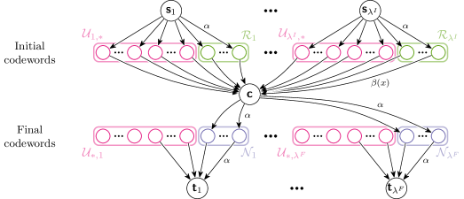
Figure 2: Information flow graph of conversion in the general case. Unchanged, retired, and new nodes are shown in different colors. Notice that each unchanged node in this figure is drawn twice: once in the initial codewords and once in the final codewords. These correspond to exactly the same node, but are drawn twice for clarity. Some representative edges are labeled with their capacities.

Thus, the information flow graph for a convertible code comprises the following nodes:

• unchanged nodes $\mathcal{U}_{{i},{j}}=\{u_{{i},{j},{1}},\ldots,u_{{i},{j},{|\mathcal{U}_{{i},{j}}|}}\}$ for all $i\in[\lambda^{I}],\ j\in[\lambda^{F}]$, which are present both in the initial and final codewords;

• retired nodes $\mathcal{R}_{i}=\{v_{{i},{1}},\ldots,v_{{i},{|\mathcal{R}_{i}|}}\}$ for $i\in[\lambda^{I}]$, which are only present in the initial codewords;

• new nodes $\mathcal{N}_{j}=\{w_{{j},{1}},\ldots,w_{{j},{|\mathcal{N}_{j}|}}\}$ for $j\in[\lambda^{F}]$, which are only present in the final codewords;

• source nodes $s_{i}$ for $i\in[\lambda^{I}]$, representing the data to be encoded;

• sink nodes $t_{j}$ for $j\in[\lambda^{F}]$, representing the data decoded; and

• a coordinator node $c$.

In the information flow graph, information source $X_{l}$ is generated at node $s_{i}$ if and only if $l\in{{P^{I}_{i}}}$, and recovered at node $t_{l}$ if and only if $l\in{{P^{F}_{j}}}$.

Throughout this paper, we use the disjoint union symbol $\sqcup$ when appropriate to emphasize that the two sets in the union are disjoint. To simplify the notation, when $*$ is used as an index, it denotes the disjoint union of the indexed set over the range of that index, e.g. $\mathcal{U}_{{*},{j}}=\bigsqcup_{i=1}^{\lambda^{I}}\mathcal{U}_{{i},{j}}$.

The information flow graph must be such that the following conditions hold: (1) the number of nodes per initial codeword is $n^{I}$, i.e., $|\mathcal{U}_{{i},{*}}|+|\mathcal{R}_{i}|=n^{I}$ for all $i\in[\lambda^{I}]$; and (2) the number of nodes per final codeword is $n^{F}$, i.e., $|\mathcal{U}_{{*},{j}}|+|\mathcal{N}_{j}|=n^{F}$ for all $j\in[\lambda^{F}]$. Additionally, the information flow graph contains the following set of edges $E$, where a directed edge from node $u$ to $v$ with capacity $\delta$ is represented with the triple $(u,v,\delta)$:

• $\{(s_{i},x,\alpha):x\in\mathcal{U}_{{i},{*}}\sqcup\mathcal{R}_{i}\}\subset E$ for each $i\in[\lambda^{I}]$, where the capacity corresponds to the size of the data stored on each node;

• $\{(x,c,\beta\!\left({x}\right)):x\in\mathcal{U}_{{i},{*}}\sqcup\mathcal{R}_{i}\}\subset E$ for each $i\in[\lambda^{I}]$, where the capacity corresponds to the amount of data downloaded from node $x$;

• $\{(c,y,\alpha):y\in\mathcal{N}_{j}\}\subset E$ for each $j\in[\lambda^{F}]$, where the capacity corresponds to the size of the data stored on each new node;

• $\{(y,t_{j},\alpha):y\in V_{j}\}\subset E$ for $V_{j}\subseteq\mathcal{U}_{{*},{j}}\sqcup\mathcal{N}_{j}$ such that $|V_{j}|=k^{F}$, for all $j\in[\lambda^{F}]$, where the capacity corresponds to the size of the data stored on each node.

The sinks $t_{j}$ represent the decoding constraints of the final code, and each choice of set $V_{j}$ will represent a different choice $k$ code symbols for decoding the final codeword. A necessary condition for a conversion procedure is to satisfy all sinks $t_{j}$ for all possible $V_{1},\ldots,V_{\lambda^{F}}$. The sets $\mathcal{U}_{{i},{j}},\mathcal{R}_{i},\mathcal{N}_{j}$ and the capacities $\beta\!\left({x}\right)$ are determined by the conversion procedure of the convertible code. Figure 2 shows the information flow graph of an arbitrary convertible code.

Definition 2 (Conversion bandwidth).

The conversion bandwidth $\gamma$ is the total network bandwidth used during conversion and is equal to the total amount of data that is transferred to the coordinator node $c$ from the initial nodes plus the total amount of data transferred to the new nodes from the coordinator node $c$, that is:

$$\gamma=\beta\!\left({\mathcal{U}_{{*},{*}}\sqcup\mathcal{R}_{*}}\right)+|\mathcal{N}_{*}|\alpha.$$ (1)

Once the structure of the graph is set and fixed, information flow analysis gives lower bounds on the capacities $\beta\!\left({x}\right)$. Therefore, a part of our objective in designing convertible codes is to set $\mathcal{U}_{{i},{j}},\mathcal{R}_{i},\mathcal{N}_{j}$ so as to minimize the lower bound on $\gamma$.

Remark 1.

In practice, conversion bandwidth can sometimes be further reduced by placing the coordinator node along with a new node and/or a retired node in the same server. One can even first split the coordinator node into several coordinator nodes, each processing data which is not used in conjunction with data processed by other coordinator nodes, and then place them in the same server as a new node and/or a retired node. Such “optimizations” do not fundamentally alter our result, and hence are left out in order to make the exposition clear.

IV Optimizing network bandwidth of conversion in the merge regime

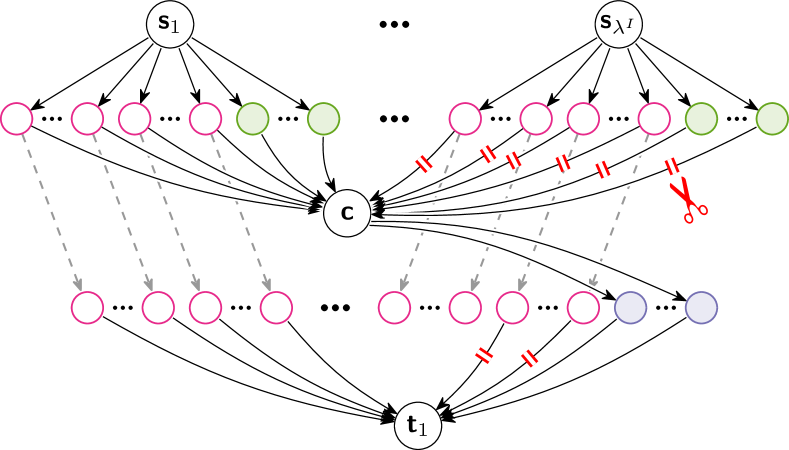
(a)

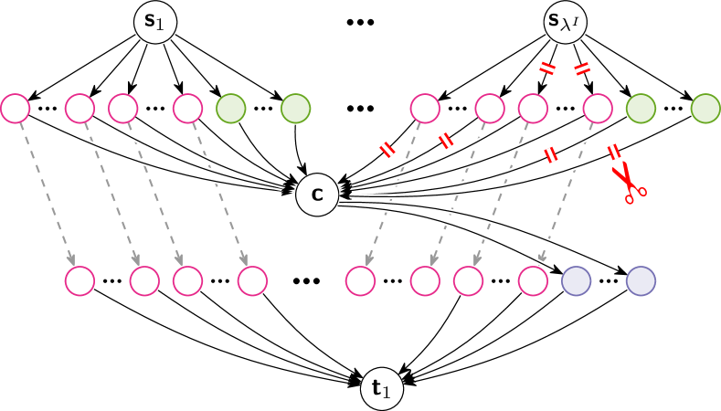
(b)

Figure 3: Information flow graph of conversion in the merge regime with two different cuts (used in proofs). For clarity, each unchanged node is drawn twice: once in the initial codewords and once in the final codeword. These two instances are connected by a dashed arrow. Marked edges denote a graph cut.

In this section, we use the information flow model presented in Section III to derive a lower bound on the conversion bandwidth for MDS codes in the merge regime. Recall from Section II-B, that convertible codes in the merge regime are those where $k^{F}=\varsigma k^{I}$ for some integer $\varsigma\geq 2$, i.e., this regime corresponds to conversions were multiple initial codewords are merged into a single final codeword. As in the previous section, our analysis focuses on a single conversion, and thus a single value for the final parameters $n^{F}$ and $k^{F}$. The lower bound on conversion bandwidth derived in this section continues to hold even when we consider multiple possible values for the final parameters $n^{F}$ and $k^{F}$.

Consider an $({n^{I}},\allowbreak{k^{I}};\allowbreak{n^{F}},\allowbreak{\varsigma k^{I}})$ convertible code in the merge regime, for some integer $\varsigma\geq 2$. Note that for all convertible codes in the merge regime, it holds that $\lambda^{I}=\varsigma$ and $\lambda^{F}=1$. Since all initial and final partitions $(\mathcal{P}_{I},\mathcal{P}_{F})$ are equivalent up to relabeling in this regime (by Proposition 1 [6]), we can omit them from our analysis. Note also that every information source shares the same sink, as there is only a single sink $t_{1}$. Thus, we may treat each source $s_{i}$ as having a single information source $X_{i}$ of rate $\alpha k^{I}$ ($i\in[\lambda^{I}]$). Figure 3(a) shows the information flow graph for a convertible code in the merge regime.

First, we derive a general lower bound on conversion bandwidth in the merge regime by considering a simple cut in the information flow graph. Intuitively, this lower bound emerges from the fact that new nodes need to have a certain amount of information from each initial codeword in order to fulfill the MDS property of the final code. This lower bound depends on the number of unchanged nodes and achieves its minimum when the number of unchanged nodes is maximized. Recall from Section II-B that convertible codes with maximum number of unchanged nodes are called stable convertible codes. Thus, the derived lower bound is minimized for stable convertible codes.

Lemma 2.

Consider an MDS $({n^{I}},\allowbreak{k^{I}};\allowbreak{n^{F}},\allowbreak{\varsigma k^{I}})$ convertible code. Then $\gamma\geq\varsigma\alpha\min\{{r^{F}},k^{I}\}+{r^{F}}\alpha$, where equality is only possible for stable codes.

Proof.

We prove this inequality via an information flow argument. Let $i\in[\lambda^{I}]$ and consider the information source generated at source $s_{i}$. Let $S\subseteq\mathcal{U}_{{i},{1}}$ be a subset of unchanged nodes from initial codeword $i$ of size $\tilde{r}_{i}=\min\{{r^{F}},|\mathcal{U}_{{i},{1}}|\}$. Consider a sink $t_{1}$ that connects to nodes $\mathcal{U}_{{*},{1}}\setminus S$. We choose the graph cut defined by nodes $\{s_{i}\}\sqcup\mathcal{U}_{{i},{1}}\sqcup\mathcal{R}_{i}$ (see Figure 3(a), which depicts the cut for $i=\lambda^{I}$). This cut yields the following inequality:

$$k^{I}\alpha\leq\max\{|\mathcal{U}_{{i},{1}}|-{r^{F}},0\}\alpha+\beta\!\left({\mathcal{U}_{{i},{1}}\sqcup\mathcal{R}_{i}}\right)$$

$$\iff\beta\!\left({\mathcal{U}_{{i},{1}}\sqcup\mathcal{R}_{i}}\right)\geq(k^{I}+{r^{F}}-\max\{|\mathcal{U}_{{i},{1}}|,{r^{F}}\})\alpha$$

By summing this inequality over all sources $i\in[\lambda^{I}]$ and using the definition of $\gamma$ (Equation 1), we obtain:

$$\gamma\geq\sum_{i=1}^{\lambda^{I}}(k^{I}+{r^{F}}-\max\{|\mathcal{U}_{{i},{1}}|,{r^{F}}\})\alpha+|\mathcal{N}_{1}|\alpha$$

By Proposition 2[6], $|\mathcal{U}_{{i},{1}}|\leq k^{I}$. Therefore, it is clear that the right hand side achieves its minimum if and only $|\mathcal{U}_{{i},{1}}|=k^{I}$ for all $i\in[\lambda^{I}]$, proving the result. ∎

Remark 2.

Note that the conversion bandwidth lower bound described in Lemma 2 coincides with the access-cost lower bound described in Theorem 1 when $r^{I}\geq{r^{F}}$. This follows by recalling that each node corresponds to an $\alpha$-length vector, and for scalar codes $\alpha=1$.

In particular, this implies that convertible codes in the merge regime which are access-optimal and have $r^{I}\geq{r^{F}}$ are also bandwidth-optimal. Observe that this corresponds to Regime 1. However, as we will show next, this property fails to hold when $r^{I}<{r^{F}}$ (that is, Regime 2).

We next derive a lower bound on conversion bandwidth which is tighter than Lemma 2 when $r^{I}<{r^{F}}$. Nevertheless, it allows for less conversion bandwidth usage than the access-optimal codes.

Intuitively, the data downloaded from retired nodes during conversion will be “more useful” than the data downloaded from unchanged nodes, since unchanged nodes already form part of the final codeword. At the same time, it is better to have the maximum amount of unchanged nodes per initial codeword ($k^{I}$) because this minimizes the number of new nodes that need to be constructed. However, this leads to fewer retired nodes per initial codeword ($r^{I}$). If the number of retired nodes per initial codeword is less than the number of new nodes ($r^{I}<{r^{F}}$), then conversion procedures are forced to download data from unchanged nodes. This is because one needs to download at least ${r^{F}}\alpha$ from each initial codeword (by Lemma 2). Since data from unchanged nodes is “less useful”, more data needs to be downloaded in order to construct the new nodes.

As in the case of Lemma 2, this lower bound depends on the number of unchanged nodes in each initial codeword, and achieves its minimum in the case of stable convertible codes.

Lemma 3.

Consider an MDS $({n^{I}},\allowbreak{k^{I}};\allowbreak{n^{F}},\allowbreak{\varsigma k^{I}})$ convertible code, with $r^{I}<{r^{F}}\leq k^{I}$. Then $\gamma\geq\varsigma\alpha\left(r^{I}+k^{I}\left(1-\frac{r^{I}}{{r^{F}}}\right)\right)+{r^{F}}\alpha$, where equality is only possible for stable codes.

Proof.

We prove this via an information flow argument. Let $i\in[\lambda^{I}]$ and consider the information source generated at source $s_{i}$. Let $S\subseteq\mathcal{U}_{{i},{1}}$ be a subset of size $\tilde{r}_{i}=\min\{{r^{F}},|\mathcal{U}_{{i},{1}}|\}$. Consider a sink $t_{1}$ that connects to the nodes in $\mathcal{U}_{{*},{1}}\setminus S$. We choose the graph cut defined by nodes $\{s_{i}\}\sqcup S\sqcup\mathcal{R}_{i}$ (see Figure 3(b), which depicts the cut when $i=\lambda^{I}$). This yields the following inequality:

$$k^{I}\alpha\leq(|\mathcal{U}_{{i},{1}}|-\tilde{r}_{i})\alpha+\beta\!\left({S}\right)+\beta\!\left({\mathcal{R}_{i}}\right).$$

By rearranging this inequality and summing over all possible choices of subset $S$, we obtain the following inequality:

$$\binom{|\mathcal{U}_{{i},{1}}|}{\tilde{r}_{i}}(k^{I}+\tilde{r}_{i}-|\mathcal{U}_{{i},{1}}|)\alpha\leq\binom{|\mathcal{U}_{{i},{1}}|-1}{\tilde{r}_{i}-1}\beta\!\left({\mathcal{U}_{{i},{1}}}\right)+\binom{|\mathcal{U}_{{i},{1}}|}{\tilde{r}_{i}}\beta\!\left({\mathcal{R}_{i}}\right)$$

$$\iff|\mathcal{U}_{{i},{1}}|(k^{I}+\tilde{r}_{i}-|\mathcal{U}_{{i},{1}}|)\alpha\leq\tilde{r}_{i}\beta\!\left({\mathcal{U}_{{i},{1}}}\right)+|\mathcal{U}_{{i},{1}}|\beta\!\left({\mathcal{R}_{i}}\right).$$ (2)

Then, our strategy to obtain a lower bound is to find the minimum value for conversion bandwidth $\gamma$ which satisfies Equation 2 for all $i\in[\lambda^{I}]$, which can be formulated as the following optimization problem:

$$\begin{array}[]{rl}\text{minimize}&\gamma=\sum_{i\in\lambda^{I}}\left[\beta\!\left({\mathcal{U}_{{i},{1}}}\right)+\beta\!\left({\mathcal{R}_{i}}\right)\right]+|\mathcal{N}_{1}|\alpha\\ \text{subject to}&\text{\lx@cref{creftype~refnum}{eq:merge-flow}, for all $i\in[\lambda^{I}]$}\\ &0\leq\beta\!\left({x}\right)\leq\alpha,\text{ for all }x\in\mathcal{U}_{{*},{1}}\sqcup\mathcal{R}_{*}.\end{array}$$ (3)

Intuitively, this linear program shows that it is preferable to download more data from retired nodes ($\beta\!\left({\mathcal{R}_{i}}\right)$) than unchanged nodes ($\beta\!\left({\mathcal{U}_{{i},{1}}}\right)$), since both have the same impact on $\gamma$ but the contribution $\beta\!\left({\mathcal{R}_{i}}\right)$ towards satisfying Equation 2 is greater than or equal than that of $\beta\!\left({\mathcal{R}_{i}}\right)$, because $\tilde{r}_{i}\leq|\mathcal{U}_{{i},{1}}|$ by definition. Thus to obtain an optimal solution we first set $\beta\!\left({\mathcal{R}_{i}}\right)=\min\{k^{I}+\tilde{r}_{i}-|\mathcal{U}_{{i},{1}}|,|\mathcal{R}_{i}|\}\alpha$ to the maximum needed for all $i\in[\lambda^{I}]$, and then set:

$$\sum_{x\in\mathcal{U}_{{i},{1}}}\beta\!\left({x}\right)=\frac{\max\{\tilde{r}_{i}-r^{I},0\}|\mathcal{U}_{{i},{1}}|\alpha}{\tilde{r}_{i}},\qquad\text{for all }i\in[\lambda^{I}]$$

to satisfy the constraints. It is straightforward to check that this solution satisfies the KKT (Karush-Kuhn-Tucker) conditions, and thus is an optimal solution to Equation 3. By replacing these terms back into $\gamma$ and simplifying we obtain the optimal objective value:

$$\gamma^{*}=\sum_{i=1}^{\lambda^{I}}\left[k^{I}-\min\{r^{I},\tilde{r}_{i}\}\left(\frac{|\mathcal{U}_{{i},{1}}|}{\tilde{r}_{i}}-1\right)\right]\alpha+|\mathcal{N}_{1}|\alpha$$

It is easy to show that the right hand side achieves its minimum if and only if $|\mathcal{U}_{{i},{1}}|=k^{I}$ for all $i\in[\lambda^{I}]$ (i.e., the code is stable). This gives the following lower bound for conversion bandwidth:

$$\gamma\geq\lambda^{I}\alpha\left(r^{I}+k^{I}\left(1-\frac{r^{I}}{{r^{F}}}\right)\right)+{r^{F}}\alpha.$$

∎

By combining Lemmas 2 and 3 we obtain the following general lower bound on conversion bandwidth of MDS convertible codes in the merge regime.

Theorem 4.

For any MDS $({n^{I}},\allowbreak{k^{I}};\allowbreak{n^{F}},\allowbreak{\varsigma k^{I}})$ convertible code:

$$\gamma\geq\begin{cases}\varsigma\alpha\min\{k^{I},{r^{F}}\}+{r^{F}}\alpha,&\text{if }r^{I}\geq{r^{F}}\text{ or }k^{I}\leq{r^{F}}\\ \varsigma\alpha\left(r^{I}+k^{I}\left(1-\frac{r^{I}}{{r^{F}}}\right)\right)+{r^{F}}\alpha,&\text{otherwise}\end{cases}$$

where equality can only be achieved by stable convertible codes.

Proof.

Follows from Lemmas 2 and 3. ∎

In Section V, we show that the lower bound of Theorem 4 is indeed achievable for all parameter values in the merge regime, and thus it is tight. We will refer to convertible codes that meet this bound with equality as bandwidth-optimal.

Remark 3.

Observe that the model above allows for nonuniform data download during conversion, that is, it allows the amount of data downloaded from each node during conversion to be different. If instead one were to assume uniform download, i.e. $\beta\!\left({x}\right)=\beta\!\left({y}\right)$ for all $x,y\in\mathcal{U}_{{*},{*}}\sqcup\mathcal{R}_{*}$, then a higher lower bound for conversion bandwidth $\gamma$ is obtained (mainly due to Equation 2 in the proof of Lemma 3). Since the lower bound of Theorem 4 is achievable, this implies that assuming uniform download necessarily leads to a suboptimal solution.

Remark 4.

The case where $k^{I}=k^{F}$ can be analyzed using the same techniques used in this section. In this case, $\lambda^{I}=\varsigma=1$. There are some differences compared to the case of the merge regime: for example, in this case the number of unchanged nodes can be at most $\min\{n^{I},n^{F}\}$ (in contrast to the $\varsigma k^{I}$ maximum of the merge regime). So, conversion bandwidth in the case where $n^{I}\geq n^{F}$ is zero, since we can simply keep $n^{F}$ nodes unchanged. In the case where $n^{I}<n^{F}$, the same analysis from Lemma 3 is followed, but the larger number of unchanged nodes will lead to a slightly different inequality. Thus, in the case of $k^{I}=k^{F}$ the lower bound on conversion bandwidth is:

$$\gamma\geq\begin{cases}0,&\text{if $n^{I}\geq n^{F}$}\\ \alpha\left(k^{I}+r^{I}\right)\left(1-\frac{r^{I}}{{r^{F}}}\right)+({r^{F}}-r^{I})\alpha,&\text{otherwise.}\end{cases}$$

Readers familiar with regenerating codes might notice that the above lower bound is equivalent to the lower bound on the repair bandwidth [8, 39] when $({r^{F}}-r^{I})$ symbols of an $[k^{I}+{r^{F}},k^{I}]$ MDS code are to be repaired with the help of the remaining $(k^{I}+r^{I})$ symbols. Note that this setting imposes a relaxed requirement of repairing only a specific subset of symbols as compared to regenerating codes which require optimal repair of all nodes. Yet, the lower bound remains the same. This is not surprising though, since it has been shown [22] that the regenerating codes lower bound for MDS codes applies even for repair of only a single specific symbol.

V Explicit construction of Bandwidth-optimal MDS convertible codes in
the merge regime

In this section, we present an explicit construction for bandwidth-optimal convertible codes in the merge regime. Our construction employs the Piggybacking framework [9]. Recall from Section II-D that the Piggybacking framework is a framework for constructing vector codes using an existing code as a base code and adding specially designed functions called piggybacks which impart additional properties to the resulting code. We use an access-optimal convertible code to construct the base code and design the piggybacks to help achieve minimum conversion bandwidth. First, in Section V-A, we describe our construction of bandwidth-optimal convertible codes in the case where we only consider fixed unique values for the final parameters $n^{F}$ and $k^{F}=\varsigma k^{I}$. Then, in Section V-B, we show that initial codes built with this construction are not only $({n^{F}},{k^{F}})$-bandwidth-optimally convertible, but also simultaneously bandwidth-optimally convertible for multiple other values of the pair $(n^{F},k^{F})$. Additionally, we present a construction which given any finite set of possible final parameter values $(n^{F},k^{F})$, constructs an initial $[n^{I},k^{I}]$ code which is simultaneously $({n^{F}},{k^{F}})$-bandwidth-optimally convertible for every $(n^{F},k^{F})$ in that set.

V-A Bandwidth-optimal MDS convertible codes for fixed final parameters

The case where ${r^{F}}\geq k^{I}$ is trivial, since the default approach to conversion is bandwidth-optimal in this case. Therefore, in the rest of this section, we only consider ${r^{F}}<k^{I}$. Moreover, in the case where $r^{I}\geq{r^{F}}$ (Regime 2), access-optimal convertible codes (for which explicit constructions are known) are also bandwidth-optimal. Therefore, we focus on the case $r^{I}<{r^{F}}$ (Regime 1).

We start by describing the base code used in our construction, followed by the design of piggybacks, and then describe the conversion procedure along with the role of piggybacks during conversion.

Base code for piggybacking

As the base code for our construction, we use a punctured initial code of an access-optimal $({k^{I}+{r^{F}}},\allowbreak{k^{I}};\allowbreak{n^{F}},\allowbreak{k^{F}})$ convertible code. Any access-optimal convertible code can be used. However, as mentioned in Section II-B, we assume without loss of generality that this convertible code is: (1) systematic, (2) linear, and (3) only requires accessing the first ${r^{F}}$ parities from each initial codeword during access-optimal conversion. We refer to the $[k^{I}+{r^{F}},k^{I}]$ initial code of this access-optimal convertible code as ${\mathcal{C}^{I}}^{\prime}$, to its $[n^{F},k^{F}]$ final code as ${\mathcal{C}^{F}}^{\prime}$. Let ${\mathcal{C}^{I}}^{\prime\prime}$ be the punctured version of ${\mathcal{C}^{I}}^{\prime}$ where the last $({r^{F}}-r^{I})$ parity symbols are punctured.

$$\begin{array}[]{|c|c|}\lx@intercol\hfil\text{initial codeword\ }1\ ({\mathcal{C}^{I}})\hfil\lx@intercol\\ \hline\cr a_{1}&b_{1}\\ \hline\cr\vbox{\hbox{.}\hbox{.}\hbox{.} }&\vbox{\hbox{.}\hbox{.}\hbox{.} }\\ \hline\cr a_{4}&b_{4}\\ \hline\cr\mathbf{a}^{\scaleto{(1)}{6pt}}\mathbf{p}_{1}^{I}&\mathbf{b}^{\scaleto{(1)}{6pt}}\mathbf{p}_{1}^{I}{\color[rgb]{0.8515625,0.37109375,0.0078125}{}+\mathbf{a}^{\scaleto{(1)}{6pt}}\mathbf{p}_{2}^{I}}\\ \hline\cr\end{array}\quad\begin{array}[]{|c|c|}\lx@intercol\hfil\text{initial codeword\ }2\ ({\mathcal{C}^{I}})\hfil\lx@intercol\\ \hline\cr a_{5}&b_{5}\\ \hline\cr\vbox{\hbox{.}\hbox{.}\hbox{.} }&\vbox{\hbox{.}\hbox{.}\hbox{.} }\\ \hline\cr a_{8}&b_{8}\\ \hline\cr\mathbf{a}^{\scaleto{(2)}{6pt}}\mathbf{p}_{1}^{I}&\mathbf{b}^{\scaleto{(2)}{6pt}}\mathbf{p}_{1}^{I}{\color[rgb]{0.8515625,0.37109375,0.0078125}{}+\mathbf{a}^{\scaleto{(2)}{6pt}}\mathbf{p}_{2}^{I}}\\ \hline\cr\end{array}\quad\begin{array}[]{|c|c|}\lx@intercol\hfil\text{final codeword\ }({\mathcal{C}^{F}})\hfil\lx@intercol\\ \hline\cr a_{1}&b_{1}\\ \hline\cr\vbox{\hbox{.}\hbox{.}\hbox{.} }&\vbox{\hbox{.}\hbox{.}\hbox{.} }\\ \hline\cr a_{4}&b_{4}\\ \hline\cr a_{5}&b_{5}\\ \hline\cr\vbox{\hbox{.}\hbox{.}\hbox{.} }&\vbox{\hbox{.}\hbox{.}\hbox{.} }\\ \hline\cr a_{8}&b_{8}\\ \hline\cr\mathbf{a}\mathbf{p}_{1}^{F}&\mathbf{b}\mathbf{p}_{1}^{F}\\ \hline\cr{\color[rgb]{0.8515625,0.37109375,0.0078125}\mathbf{a}\mathbf{p}_{2}^{F}}&\mathbf{b}\mathbf{p}_{2}^{F}\\ \hline\cr\end{array}$$

Figure 4: Example of a bandwidth-optimal $({5},\allowbreak{4};\allowbreak{10},\allowbreak{8})$ convertible code. Each block in this diagram represents a codeword, where each column corresponds to a distinct coordinate of the $\alpha$-length vector ($\alpha=2$ in this case), and each row corresponds to a node. The shaded rows correspond to retired nodes for the first two blocks (initial codewords), and new nodes for the third block (final codeword). For the initial codewords, text color is used emphasize the piggybacks. In the final codeword, text color is used to denote the base code symbol which can be directly computed from the piggybacks.

Piggyback design

Now, we describe how to construct the $[n^{I},k^{I},\alpha]$ initial vector code ${\mathcal{C}^{I}}$ and the $[n^{F},k^{F},\alpha]$ final vector code ${\mathcal{C}^{F}}$ that make up the bandwidth-optimal $({n^{I}},\allowbreak{k^{I}};\allowbreak{n^{F}},\allowbreak{\varsigma k^{I}})$ convertible code.

The first step is to choose the value of $\alpha$. Let us reexamine the lower bound derived in Theorem 4 for $r^{I}<{r^{F}}<k^{I}$, which is rewritten below in a different form.

$$\gamma\geq\lambda^{I}\left(r^{I}\alpha+k^{I}\left(1-\frac{r^{I}}{{r^{F}}}\right)\alpha\right)+{r^{F}}\alpha.$$

We can see that one way to achieve this lower bound would be to download exactly $\beta_{1}=\alpha$ subsymbols from each of the $r^{I}$ retired nodes in the $\lambda^{I}$ initial codewords, and to download $\beta_{2}=\left(1-\nicefrac{{r^{I}}}{{{r^{F}}}}\right)\alpha$ subsymbols from each of the $k^{I}$ unchanged nodes in the $\lambda^{I}$ initial stripes. Thus, we choose $\alpha={r^{F}}$, which is the smallest value that makes $\beta_{1}$ and $\beta_{2}$ integers, thus making:

$$\beta_{1}={r^{F}}\qquad\text{and}\qquad\beta_{2}=({r^{F}}-r^{I}).$$

The next step is to design the piggybacks. We first provide the intuition behind the design. Recall from above that we can download $\beta_{2}=({r^{F}}-r^{I})$ subsymbols from each unchanged node and all the $\alpha$ subsymbols from each retired node. Hence, we can utilize up to $\beta_{2}=({r^{F}}-r^{I})$ coordinates from each of the $r^{I}$ parity nodes for piggybacking. Given that there are precisely $({r^{F}}-r^{I})$ punctured symbols and $\alpha$ instances of ${\mathcal{C}^{I}}^{\prime\prime}$, we can store piggybacks corresponding to $r^{I}$ instances of each of these punctured symbols. During conversion, these punctured symbols can be reconstructed and used for constructing the new nodes.

Consider a message $\mathbf{m}\in\mathbb{F}_{q}^{\lambda^{I}k^{I}\alpha}$ split into $\lambda^{I}\alpha$ submessages $\mathbf{m}^{({s})}_{j}\in\mathbb{F}_{q}^{k^{I}}$, representing the data encoded by instance $j\in[\alpha]$ of the base code in initial codeword $s\in[\lambda^{I}]$. Recall that ${\mathcal{C}^{I}}^{\prime\prime}$ is systematic by construction. Therefore, the submessage $\mathbf{m}^{({s})}_{j}$ will correspond to the contents of the $j$-th coordinate of the $k^{I}$ systematic nodes in initial codeword $s$. Let $c^{I}_{{i},{j}}(s)$ denote the contents of the $j$-th coordinate of parity symbol $i$ in initial codeword $s$ under code ${\mathcal{C}^{I}}$, and $c^{F}_{{i},{j}}$ let denote the same for the single final codeword encoded under ${\mathcal{C}^{F}}$. These are constructed as follows:

$$c^{I}_{{i},{j}}(s) =\begin{cases}\mathbf{m}^{({s})}_{j}\mathbf{p}^{I}_{i},&\text{for }s\in[\lambda^{I}],\;i\in[r^{I}],\;1\leq j\leq r^{I}\\ \mathbf{m}^{({s})}_{j}\mathbf{p}^{I}_{i}+\mathbf{m}^{({s})}_{i}\mathbf{p}^{I}_{j},&\text{for }s\in[\lambda^{I}],\;i\in[r^{I}],\;r^{I}<j\leq{r^{F}}\end{cases}$$

$$c^{F}_{{i},{j}} =[\mathbf{m}^{({1})}_{j}\cdots\mathbf{m}^{({\lambda^{I}})}_{j}]\mathbf{p}^{F}_{i},\qquad\text{for }i\in[{r^{F}}],\;j\in[{r^{F}}],$$

where $\mathbf{p}^{I}_{i}$ corresponds to the encoding vector of the $i$-th parity of ${\mathcal{C}^{I}}^{\prime}$ and $\mathbf{p}^{F}_{i}$ corresponds to the encoding vector of the $i$-th parity of ${\mathcal{C}^{F}}^{\prime}$. By using the access-optimal conversion procedure from the base code, we can compute $c^{F}_{{i},{j}}=[\mathbf{m}^{({1})}_{j}\cdots\mathbf{m}^{({\lambda^{I}})}_{j}]\mathbf{p}^{F}_{i}$ from $\{\mathbf{m}^{({s})}_{j}\mathbf{p}^{I}_{i}:s\in[\lambda^{I}]\}$ for all $i\in[{r^{F}}]$ and $j\in[{r^{F}}]$. Notice that each initial codeword is independent and encoded in the same way (as required).

This piggybacking design, that of using parity code symbols of the base code as piggybacks, is inspired by one of the piggybacking designs proposed in [9], where it is used for efficiently reconstructing failed (parity) code symbols.

Conversion procedure

Conversion proceeds as follows:

1. Download $D=\{\mathbf{m}^{({s})}_{j}:s\in[\lambda^{I}]\text{ and }r^{I}<j\leq{r^{F}}\}$, $C_{1}=\{c^{I}_{{i},{j}}(s):s\in[\lambda^{I}],\ i\in[r^{I}],\text{ and }1\leq j\leq r^{I}\}$, and $C_{2}=\{c^{I}_{{i},{j}}(s):s\in[\lambda^{I}],\ i\in[r^{I}],\text{ and }r^{I}<j\leq{r^{F}}\}$.

2. Recover the piggybacks $C_{3}=\{\mathbf{m}^{({s})}_{j}\mathbf{p}^{I}_{i}:s\in[\lambda^{I}],\ r^{I}<i\leq{r^{F}},\text{ and }1\leq j\leq r^{I}\}$ by computing $\mathbf{m}^{({s})}_{i}\mathbf{p}^{I}_{j}$ from $D$ and obtaining $\mathbf{m}^{({s})}_{j}\mathbf{p}^{I}_{i}=c^{I}_{{j},{i}}(s)-\mathbf{m}^{({s})}_{i}\mathbf{p}^{I}_{j}$ using $C_{2}$.

3. Compute the remaining base code symbols from the punctured symbols $C_{4}=\{\mathbf{m}^{({s})}_{i}\mathbf{p}^{I}_{j}:s\in[\lambda^{I}],\ r^{I}<i\leq{r^{F}},\text{ and }r^{I}<j\leq{r^{F}}\}$ using $D$.

4. Compute the parity nodes of the final codeword specified by the subsymbols $C_{5}=\{c^{F}_{{i},{j}}:i\in[{r^{F}}],\ j\in[{r^{F}}]\}$. This is done by using the conversion procedure from the access-optimal convertible code used as base code to compute $C_{5}$ from $C_{1},\ C_{2},\ C_{3},$ and $C_{4}$.

This procedure requires downloading $\beta_{1}$ subsymbols from each retired node and $\beta_{2}$ subsymbols from each unchanged node. Additionally, ${r^{F}}\alpha$ network bandwidth is required to write the new nodes. Thus, the total network bandwidth of conversion is:

$$\gamma =\lambda^{I}\left(r^{I}\beta_{1}+k^{I}\beta_{2}\right)+{r^{F}}\alpha$$

$$=\lambda^{I}\left(r^{I}\alpha+k^{I}\left(1-\frac{r^{I}}{{r^{F}}}\right)\right)+{r^{F}}\alpha$$

which matches Theorem 4.

Now we show a concrete example of our construction.

Example 1 (Bandwidth-optimal conversion in the merge regime).

Suppose we want to construct a bandwidth-optimal $({5},\allowbreak{4};\allowbreak{10},\allowbreak{8})$ convertible code over a finite field $\mathbb{F}_{q}$ (assume that $q$ is sufficiently large). As a base code, we use a punctured access-optimal $({6},\allowbreak{4};\allowbreak{10},\allowbreak{8})$ convertible code. Thus, ${\mathcal{C}^{I}}^{\prime}$ is a $[6,4]$ code, ${\mathcal{C}^{F}}^{\prime}$ is a $[10,8]$ code, and ${\mathcal{C}^{I}}^{\prime\prime}$ is a $[5,4]$ code, all derived from the chosen access-optimal convertible code as described in the construction above. Let $\mathbf{p}_{1}^{I},\mathbf{p}_{2}^{I}\in\mathbb{F}_{q}^{4\times 1}$ be the encoding vectors for the parities of ${\mathcal{C}^{I}}^{\prime}$, and $\mathbf{p}_{1}^{F},\mathbf{p}_{2}^{F}\in\mathbb{F}_{q}^{8\times 1}$ be the encoding vector for the parities of ${\mathcal{C}^{F}}^{\prime}$.

Since $\alpha=2$, we construct a $[5,4,2]$ initial vector code ${\mathcal{C}^{I}}$ and a $[10,8,2]$ final vector code ${\mathcal{C}^{F}}$. Let $\mathbf{a}=(a_{1},\ldots,a_{8})$ and $\mathbf{b}=(b_{1},\ldots,b_{8})$. Figure 4 shows the resulting piggybacked codes encoding submessages $\mathbf{a}^{(1)}=(a_{1},\ldots,a_{4}),\mathbf{a}^{(2)}=(a_{5},\ldots,a_{8}),\mathbf{b}^{(1)}=(b_{1},\ldots,b_{4}),\mathbf{b}^{(2)}=(b_{5},\ldots,b_{8})\in\mathbb{F}_{q}^{1\times 4}$.

During conversion, only 12 subsymbols need to be downloaded: $\mathbf{b}^{(1)},\mathbf{b}^{(2)}$ and all the parity symbols from both codewords. From these subsymbols, we can recover the piggyback terms $\mathbf{a}^{(1)}\mathbf{p}_{2}^{I}$ and $\mathbf{a}^{(2)}\mathbf{p}_{2}^{I}$, and then compute $\mathbf{b}^{(1)}\mathbf{p}_{2}^{I}$ and $\mathbf{b}^{(2)}\mathbf{p}_{2}^{I}$ in order to reconstruct the second parity symbol of ${\mathcal{C}^{I}}^{\prime}$. Finally, we use $\mathbf{a}^{(i)}\mathbf{p}_{1}^{I},\mathbf{b}^{(i)}\mathbf{p}_{1}^{I},\mathbf{a}^{(i)}\mathbf{p}_{2}^{I},\mathbf{b}^{(i)}\mathbf{p}_{2}^{I}$ for $i\in\{1,2\}$ with the conversion procedure from the access-optimal convertible code to compute the base code symbols $\mathbf{a}\ \mathbf{p}^{F}_{1},\mathbf{a}\ \mathbf{p}^{F}_{2},\mathbf{b}\ \mathbf{p}^{F}_{1}$ and $\mathbf{b}\ \mathbf{p}^{F}_{2}$ of the new nodes.

The default approach would require one to download 16 subsymbols in total from the initial nodes. Both approaches require downloading 4 subsymbols in total from the coordinator node to the new nodes. Thus, the proposed construction leads to $20\%$ reduction in conversion bandwidth as compared to the default approach of reencoding.

V-B Convertible codes with bandwidth-optimal conversion for multiple final parameters

In practice, the final parameters $n^{F},k^{F}$ might depend on observations made after the initial encoding of the data and hence they may be unknown at code construction time. In particular, for a $({n^{I}},\allowbreak{k^{I}};\allowbreak{n^{F}},\allowbreak{\varsigma k^{I}})$ convertible code in the merge regime this means that the values of $\lambda^{I}=\varsigma$ and ${r^{F}}=(n^{F}-k^{F})$ are unknown.

To ameliorate this problem, we now present convertible codes which support bandwidth-optimal conversion simultaneously for multiple possible values of the final parameters. Recall property (4) of the access-optimal base code which we reviewed in Section II-B: when constructed with a given value of $\lambda^{I}=\varsigma$ and ${r^{F}}=r$, the initial $[n^{I},k^{I}]$ code is $({n^{F}},{k^{F}})$-access-optimally convertible for all $k^{F}=\varsigma^{\prime}k^{I}$ and $n^{F}=k^{F}+r^{\prime}$ such that $1\leq\varsigma^{\prime}\leq\varsigma$ and $1\leq r^{\prime}\leq r$.

V-B1 Supporting multiple values of $\lambda^{I}$

The construction from Section V for some particular value of $\lambda^{I}=\varsigma$, natively supports bandwidth-optimal conversion for any $\lambda^{I}=\varsigma^{\prime}<\varsigma$. This is a consequence of property (4) above, and can be done easily by considering one or multiple of the initial codewords as consisting of zeroes only, and ignoring them during conversion. From Theorem 4, it is easy to see that this modified conversion procedure achieves optimal network bandwidth cost for the new parameter $\lambda^{I}=\varsigma^{\prime}$.

V-B2 Supporting multiple values of ${r^{F}}$

We break this scenario into two cases:

Case 1 (supporting ${r^{F}}\leq r^{I}$): due to property (4) above, the base code used in the construction from Section V supports access-optimal conversion for any value of ${r^{F}}=r$ such that $r\leq r^{I}$. Using this property, one can achieve bandwidth optimality for any $r\leq r^{I}$ by simply using the access-optimal conversion on each of the $\alpha$ instances of the base code independently. The only difference is that some of the instances might have piggybacks, which can be simply ignored. The final code might still have these piggybacks, however they will still satisfy the property that the piggybacks in instance $i$ ($2\leq i\leq\alpha$) only depend on data from instances $\{1,\ldots,(i-1)\}$. Thus, the final code will have the MDS property and the desired parameters.

Case 2 (supporting ${r^{F}}>r^{I}$): for supporting multiple values of ${r^{F}}\in\{r_{1},r_{2},\ldots,r_{s}\}$ such that $r_{i}>r^{I}$ ($i\in[s]$), we start with an access-optimal convertible code having ${r^{F}}=\max_{i}r_{i}$. Then we repeat the piggybacking step of the construction (see Section V-A) for each $r_{i}$, using the resulting code from step $i$ (with the punctured symbols from ${\mathcal{C}^{I}}^{\prime}$ added back) as a base code for step $(i+1)$. Therefore, the resulting code will have $\alpha=\prod_{i=1}^{s}r_{i}$. Since the piggybacking step will preserve the MDS property of its base code, and the initial code used in the first piggyback step is MDS, it is clear that the initial code resulting from the last piggybacking step will also be MDS. Conversion for one of the supported ${r^{F}}=r_{i}$ is performed as described in Section V-A on each of the additional instances created by steps $(i+1),\ldots,s$ (i.e. $\prod_{i^{\prime}=(i+1)}^{s}r_{i^{\prime}}$ in total). As before, some of these instances after conversion will have piggybacks, which can be simply ignored, as the resulting code will continue to have the property that piggybacks from a given instance only depend on data from earlier instances.

$$\begin{array}[]{|c|c||c|c||c|c|}\lx@intercol\hfil\text{initial codeword\ }1\ ({\mathcal{C}^{I}})\hfil\lx@intercol\\ \hline\cr a_{1}&b_{1}&c_{1}&d_{1}&e_{1}&f_{1}\\ \hline\cr\vbox{\hbox{.}\hbox{.}\hbox{.} }&\vbox{\hbox{.}\hbox{.}\hbox{.} }&\vbox{\hbox{.}\hbox{.}\hbox{.} }&\vbox{\hbox{.}\hbox{.}\hbox{.} }&\vbox{\hbox{.}\hbox{.}\hbox{.} }&\vbox{\hbox{.}\hbox{.}\hbox{.} }\\ \hline\cr a_{4}&b_{4}&c_{4}&d_{4}&e_{4}&f_{4}\\ \hline\cr\mathbf{a}^{\scaleto{(1)}{6pt}}\mathbf{p}_{1}^{I}&\mathbf{b}^{\scaleto{(1)}{6pt}}\mathbf{p}_{1}^{I}{\color[rgb]{0.8515625,0.37109375,0.0078125}{}+\mathbf{a}^{\scaleto{(1)}{6pt}}\mathbf{p}_{2}^{I}}&\mathbf{c}^{\scaleto{(1)}{6pt}}\mathbf{p}_{1}^{I}{\color[rgb]{0.90625,0.16015625,0.54296875}{}+\mathbf{a}^{\scaleto{(1)}{6pt}}\mathbf{p}_{2}^{I}}&\mathbf{d}^{\scaleto{(1)}{6pt}}\mathbf{p}_{1}^{I}{\color[rgb]{0.8515625,0.37109375,0.0078125}{}+\mathbf{c}^{\scaleto{(1)}{6pt}}\mathbf{p}_{2}^{I}}{\color[rgb]{0.90625,0.16015625,0.54296875}{}+\mathbf{b}^{\scaleto{(1)}{6pt}}\mathbf{p}_{2}^{I}}&\mathbf{e}^{\scaleto{(1)}{6pt}}\mathbf{p}_{1}^{I}{\color[rgb]{0.90625,0.16015625,0.54296875}{}+\mathbf{a}^{\scaleto{(1)}{6pt}}\mathbf{p}_{3}^{I}}&\mathbf{f}^{\scaleto{(1)}{6pt}}\mathbf{p}_{1}^{I}{\color[rgb]{0.8515625,0.37109375,0.0078125}{}+\mathbf{e}^{\scaleto{(1)}{6pt}}\mathbf{p}_{2}^{I}}{\color[rgb]{0.90625,0.16015625,0.54296875}{}+\mathbf{b}^{\scaleto{(1)}{6pt}}\mathbf{p}_{3}^{I}}\\ \hline\cr\end{array}$$

$$\begin{array}[]{|c|c||c|c||c|c|}\lx@intercol\hfil\text{final codeword\ }({r^{F}}=2)\hfil\lx@intercol\\ \hline\cr a_{1}&b_{1}&c_{1}&d_{1}&e_{1}&f_{1}\\ \hline\cr\vbox{\hbox{.}\hbox{.}\hbox{.} }&\vbox{\hbox{.}\hbox{.}\hbox{.} }&\vbox{\hbox{.}\hbox{.}\hbox{.} }&\vbox{\hbox{.}\hbox{.}\hbox{.} }&\vbox{\hbox{.}\hbox{.}\hbox{.} }&\vbox{\hbox{.}\hbox{.}\hbox{.} }\\ \hline\cr a_{8}&b_{8}&c_{8}&d_{8}&e_{8}&f_{8}\\ \hline\cr\mathbf{a}\mathbf{p}_{1}^{F}&\mathbf{b}\mathbf{p}_{1}^{F}&\mathbf{c}\mathbf{p}_{1}^{F}{\color[rgb]{0.90625,0.16015625,0.54296875}{}+\mathbf{a}^{\scaleto{(1)}{6pt}}\mathbf{p}_{2}^{I}}{\color[rgb]{0.90625,0.16015625,0.54296875}{}+\mathbf{a}^{\scaleto{(2)}{6pt}}\mathbf{p}_{2}^{I}}&\mathbf{d}\mathbf{p}_{1}^{F}&\mathbf{e}\mathbf{p}_{1}^{F}{\color[rgb]{0.90625,0.16015625,0.54296875}{}+\mathbf{a}^{\scaleto{(1)}{6pt}}\mathbf{p}_{3}^{I}}{\color[rgb]{0.90625,0.16015625,0.54296875}{}+\mathbf{a}^{\scaleto{(2)}{6pt}}\mathbf{p}_{3}^{I}}&\mathbf{f}\mathbf{p}_{1}^{F}\\ \hline\cr{\color[rgb]{0.8515625,0.37109375,0.0078125}\mathbf{a}\mathbf{p}_{2}^{F}}&\mathbf{b}\mathbf{p}_{2}^{F}&{\color[rgb]{0.8515625,0.37109375,0.0078125}\mathbf{c}\mathbf{p}_{2}^{F}}&\mathbf{d}\mathbf{p}_{2}^{F}&{\color[rgb]{0.8515625,0.37109375,0.0078125}\mathbf{e}\mathbf{p}_{2}^{F}}&\mathbf{f}\mathbf{p}_{2}^{F}\\ \hline\cr\end{array}$$

$$\begin{array}[]{|c|c||c|c||c|c|}\lx@intercol\hfil\text{final codeword\ }({r^{F}}=3)\hfil\lx@intercol\\ \hline\cr a_{1}&b_{1}&c_{1}&d_{1}&e_{1}&f_{1}\\ \hline\cr\vbox{\hbox{.}\hbox{.}\hbox{.} }&\vbox{\hbox{.}\hbox{.}\hbox{.} }&\vbox{\hbox{.}\hbox{.}\hbox{.} }&\vbox{\hbox{.}\hbox{.}\hbox{.} }&\vbox{\hbox{.}\hbox{.}\hbox{.} }&\vbox{\hbox{.}\hbox{.}\hbox{.} }\\ \hline\cr a_{8}&b_{8}&c_{8}&d_{8}&e_{8}&f_{8}\\ \hline\cr\mathbf{a}\mathbf{p}_{1}^{F}&\mathbf{b}\mathbf{p}_{1}^{F}{\color[rgb]{0.8515625,0.37109375,0.0078125}{}+\mathbf{a}^{\scaleto{(1)}{6pt}}\mathbf{p}_{2}^{I}}{\color[rgb]{0.8515625,0.37109375,0.0078125}{}+\mathbf{a}^{\scaleto{(2)}{6pt}}\mathbf{p}_{2}^{I}}&\mathbf{c}\mathbf{p}_{1}^{F}&\mathbf{d}\mathbf{p}_{1}^{F}&\mathbf{e}\mathbf{p}_{1}^{F}&\mathbf{f}\mathbf{p}_{1}^{F}\\ \hline\cr{\color[rgb]{0.90625,0.16015625,0.54296875}\mathbf{a}\mathbf{p}_{2}^{F}}&{\color[rgb]{0.90625,0.16015625,0.54296875}\mathbf{b}\mathbf{p}_{2}^{F}}&\mathbf{c}\mathbf{p}_{2}^{F}&\mathbf{d}\mathbf{p}_{2}^{F}&\mathbf{e}\mathbf{p}_{2}^{F}&\mathbf{f}\mathbf{p}_{2}^{F}\\ \hline\cr{\color[rgb]{0.90625,0.16015625,0.54296875}\mathbf{a}\mathbf{p}_{3}^{F}}&{\color[rgb]{0.90625,0.16015625,0.54296875}\mathbf{b}\mathbf{p}_{3}^{F}}&\mathbf{c}\mathbf{p}_{3}^{F}&\mathbf{d}\mathbf{p}_{3}^{F}&\mathbf{e}\mathbf{p}_{3}^{F}&\mathbf{f}\mathbf{p}_{3}^{F}\\ \hline\cr\end{array}$$

Figure 5: Example of a $[5,4]$ MDS code that supports bandwidth-optimal conversion to multiple final codes (only one initial stripe is shown). This code supports bandwidth-optimal conversion to a $[8+r,8]$ MDS code for $r=1,2,3$. Text color is used in the initial codeword to denote piggybacks from different piggybacking steps. In the possible final codewords, text color is used to denote base code symbols which are directly computed from the corresponding piggybacks, or to denote leftover piggybacks which were not used during conversion.

Example 2 (bandwidth-optimal conversion for multiple final parameters).

In this example, we will extend the $({5},\allowbreak{4};\allowbreak{10},\allowbreak{8})$ convertible code from Example 1 (${r^{F}}=2$) to construct a code which additionally supports bandwidth-optimal conversion to an $[11,8]$ MDS code (${r^{F}}=3$). Figure 5 shows one initial codeword of the new initial vector code, which has $\alpha=2\cdot 3=6$. Here $\mathbf{a}^{(1)}=(a_{1},\ldots,a_{4})$, $\mathbf{a}^{(2)}=(a_{5},\ldots,a_{8})\in\mathbb{F}_{q}^{1\times 4}$, $\mathbf{a}=(a_{1},\ldots,a_{8})\in\mathbb{F}_{q}^{1\times 8}$, and similarly for $\mathbf{b},\ldots,\mathbf{f}$. The vectors $\mathbf{p}^{I}_{i}\in\mathbb{F}_{q}^{4\times 1}$ are the encoding vectors of the initial code ${\mathcal{C}^{I}}^{\prime}$ and $\mathbf{p}^{F}_{i}\in\mathbb{F}_{q}^{8\times 1}$ are encoding vectors of the final code ${\mathcal{C}^{F}}^{\prime}$ ($i\in\{1,2,3\}$). Since the maximum supported ${r^{F}}$ is 3, we start with an access-optimal $({7},\allowbreak{4};\allowbreak{11},\allowbreak{8})$ convertible code. Thus, ${\mathcal{C}^{I}}^{\prime}$ is a $[7,4]$ code, ${\mathcal{C}^{F}}^{\prime}$ is a $[11,8]$ code, and ${\mathcal{C}^{I}}^{\prime\prime}$ is a $[5,4]$ code. In the first round of piggybacking we consider ${r^{F}}=2$, which yields the code shown in Example 1. In the second round of piggybacking we consider ${r^{F}}=3$ and piggyback the code resulting from the first round, which yields the code shown in Figure 5. Conversion for ${r^{F}}=1$ proceeds by simply downloading the contents of the single parity node and using the access-optimal conversion procedure. Conversion for ${r^{F}}=2$ proceeds by treating this code as three instances of the code from Example 1 and performing conversion for each one independently. Conversion for ${r^{F}}=3$ proceeds by treating this code as a vector code with $\alpha=3$ and base field $\mathbb{F}_{q^{2}}$ (i.e. each element is a vector over $\mathbb{F}_{q}$ of length 2).

Remark 5 (Field size requirement).

The field size requirement for $\mathbb{F}_{q}$ of the constructions presented in this section is given by the field size requirement of the base code used. The currently lowest known field size requirement for an explicit construction of systematic linear access-optimal convertible codes in the merge regime is given by [6]. In general, this requirement is roughly $q\geq 2^{\varsigma(n^{I})^{3}}$. When ${r^{F}}\leq r^{I}-\varsigma+1$, the requirement can be significantly reduced to $q\geq k^{I}r^{I}$. And when ${r^{F}}\leq\lfloor\nicefrac{{r^{I}}}{{\varsigma}}\rfloor$, the requirement can be further reduced to $q\geq\max\{n^{I},n^{F}\}$.

VI Bandwidth savings of bandwidth-optimal convertible codes

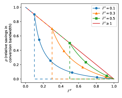
Figure 6: Achievable savings in conversion bandwidth by bandwidth-optimal convertible codes in comparison to the default approach to conversion. Here $\widetilde{r}^{I}=r^{I}/k^{I}$ and $\widetilde{r}^{F}={r^{F}}/k^{I}$ are the initial and final redundancies, divided by the initial code dimension. Each curve shows the relative savings for a fixed value of $\widetilde{r}^{I}$, as $\widetilde{r}^{F}$ varies. Solid lines indicate bandwidth-optimal convertible codes, and dashed lines indicate access-optimal convertible codes. Notice that each curve overlaps with the red curve ($\widetilde{r}^{I}\geq 1$) in the range $\widetilde{r}^{F}\in(0,\widetilde{r}^{I}]$.

In this section, we show the amount of savings in bandwidth that can be obtained by using bandwidth-optimal convertible codes in the merge regime, relative to the default approach to conversion. We present the amount of savings in terms of two ratios:

$$\widetilde{r}^{I}=(\nicefrac{{r^{I}}}{{k^{I}}})\qquad\text{and}\qquad\widetilde{r}^{F}=(\nicefrac{{{r^{F}}}}{{k^{I}}}),$$

i.e. the initial and final amount of “redundancy” relative to the initial dimension of the code. For simplicity, we only consider the bandwidth cost of communication from nodes to the coordinator node, since the bandwidth cost of communication from the coordinator node to new nodes is fixed for stable convertible codes (specifically, it is equal to $\alpha{r^{F}}$). Thus, the bandwidth cost of the default approach is always $\varsigma k^{I}\alpha$. Figure 6 shows the relative savings, i.e. the ratio between the bandwidth cost of optimal conversion and the bandwidth cost of conversion under the default approach, for fixed values of $\widetilde{r}^{I}\in(0,\infty)$ and varying $\widetilde{r}^{F}\in(0,\infty)$.

Each curve shown in Figure 6 can be divided into three regions, depending on the value of $\widetilde{r}^{F}$:

• Region $0<\widetilde{r}^{F}\leq\widetilde{r}^{I}$ and $\widetilde{r}^{F}<1$: this implies that ${r^{F}}\leq r^{I}$, so by Lemma 2 the conversion bandwidth is $\varsigma{r^{F}}\alpha$, and the relative savings are:

  $$\rho=1-\frac{\varsigma{r^{F}}\alpha}{\varsigma k^{I}\alpha}=1-\widetilde{r}^{F}.$$

  This region corresponds to Regime 2, and in this region access-optimal convertible codes are also bandwidth-optimal. This region of the curve is linear, and the amount of savings is not affected by $\widetilde{r}^{I}$.

• Region $\widetilde{r}^{I}<\widetilde{r}^{F}<1$: this implies that $r^{I}\leq{r^{F}}\leq k^{I}$, and by Lemma 3 the conversion bandwidth is $\varsigma\alpha(r^{I}+k^{I}(1-r^{I}/{r^{F}}))$, and the relative savings are:

  $$\rho=1-\frac{\varsigma\alpha\left(r^{I}+k^{I}\left(1-\frac{r^{I}}{{r^{F}}}\right)\right)}{\varsigma k^{I}\alpha}=\widetilde{r}^{I}\left(\frac{1}{\widetilde{r}^{F}}-1\right).$$

  This corresponds to Regime 1, where access-optimal convertible codes provide no conversion bandwidth savings. Thus bandwidth-optimal convertible codes provide substantial savings in conversion bandwidth in this regime, compared to access-optimal convertible codes.

• Region $\widetilde{r}^{F}\geq 1$: this implies that ${r^{F}}\geq k^{I}$ and by Lemma 2 a bandwidth of $\varsigma k^{I}\alpha$ is required. Thus no savings in bandwidth cost are possible in this region.

Thus, bandwidth-optimal convertible codes allow for savings in network bandwidth on a much broader region relative to access-optimal convertible codes.

VII Conclusions and future directions

In this paper, we initiated a study on the network bandwidth cost of convertible codes. We showed that the conversion problem can be effectively modeled using network information flow to obtain lower bounds on conversion bandwidth. Using the bounds derived, we showed that for the merge regime access-optimal convertible codes are also bandwidth-optimal when $r^{I}\geq{r^{F}}$ (Regime 1) and that there is room for reducing conversion bandwidth when $r^{I}<{r^{F}}$ (Regime 2). We proposed an explicit construction which achieves the optimal conversion bandwidth for all parameters in the merge regime. Finally, we showed that bandwidth-optimal convertible codes can achieve substantial savings in conversion bandwidth over the default approach and access-optimal convertible codes.

This work leads to several open questions and challenges. The main challenge is to extend the conversion bandwidth lower bounds and bandwidth-optimal constructions to encompass all possible parameter values (i.e. the general regime). Another important challenge is characterizing the optimal value of $\alpha$, especially in the case of multiple possible final parameter values, where $\alpha$ can become very large when using the construction proposed in this paper. Yet another open challenge is lowering the field size requirement of bandwidth-optimal convertible code constructions, as well as deriving lower bounds for their field size requirements.

References

- [1] S. Ghemawat, H. Gobioff, and S. Leung, “The Google file system,” in Proceedings of the 19th ACM Symposium on Operating Systems Principles 2003, SOSP 2003, Bolton Landing, NY, USA, October 19-22, 2003 (M. L. Scott and L. L. Peterson, eds.), pp. 29–43, ACM, 2003.
- [2] D. Borthakur, R. Schmidt, R. Vadali, S. Chen, and P. Kling, “HDFS RAID - Facebook.” Available on: http://www.slideshare.net/ydn/hdfs-raid-facebook. Accessed: 2019-07-23.
- [3] C. Huang, H. Simitci, Y. Xu, A. Ogus, B. Calder, P. Gopalan, J. Li, and S. Yekhanin, “Erasure coding in Windows Azure storage,” in 2012 USENIX Annual Technical Conference, Boston, MA, USA, June 13-15, 2012 (G. Heiser and W. C. Hsieh, eds.), pp. 15–26, USENIX Association, 2012.
- [4] Apache Software Foundation, “Apache hadoop: HDFS erasure coding.” Available on: https://hadoop.apache.org/docs/r3.0.0/hadoop-project-dist/hadoop-hdfs/HDFSErasureCoding.html. Accessed: 2019-07-23.
- [5] S. Kadekodi, K. V. Rashmi, and G. R. Ganger, “Cluster storage systems gotta have HeART: improving storage efficiency by exploiting disk-reliability heterogeneity,” in 17th USENIX Conference on File and Storage Technologies, FAST 2019, Boston, MA, February 25-28, 2019 (A. Merchant and H. Weatherspoon, eds.), pp. 345–358, USENIX Association, 2019.
- [6] F. Maturana and K. V. Rashmi, “Convertible codes: new class of codes for efficient conversion of coded data in distributed storage,” in 11th Innovations in Theoretical Computer Science Conference, ITCS 2020, January 12-14, 2020, Seattle, Washington, USA (T. Vidick, ed.), vol. 151 of LIPIcs, pp. 66:1–66:26, Schloss Dagstuhl - Leibniz-Zentrum für Informatik, 2020.
- [7] F. Maturana, V. S. C. Mukka, and K. V. Rashmi, “Access-optimal linear MDS convertible codes for all parameters,” in IEEE International Symposium on Information Theory, ISIT 2020, Los Angeles, California, USA, June 21-26, 2020, 2020.
- [8] A. G. Dimakis, B. Godfrey, Y. Wu, M. J. Wainwright, and K. Ramchandran, “Network coding for distributed storage systems,” IEEE Transactions on Information Theory, vol. 56, no. 9, pp. 4539–4551, 2010.
- [9] K. V. Rashmi, N. B. Shah, and K. Ramchandran, “A piggybacking design framework for read-and download-efficient distributed storage codes,” IEEE Transactions on Information Theory, vol. 63, no. 9, pp. 5802–5820, 2017.
- [10] R. Ahlswede, N. Cai, S. R. Li, and R. W. Yeung, “Network information flow,” IEEE Transactions on Information Theory, vol. 46, no. 4, pp. 1204–1216, 2000.
- [11] S. R. Li, R. W. Yeung, and N. Cai, “Linear network coding,” IEEE Transactions on Information Theory, vol. 49, no. 2, pp. 371–381, 2003.
- [12] R. Koetter and M. Médard, “An algebraic approach to network coding,” IEEE/ACM Transactions on Networking, vol. 11, no. 5, pp. 782–795, 2003.
- [13] T. Ho, M. Médard, R. Koetter, D. R. Karger, M. Effros, J. Shi, and B. Leong, “A random linear network coding approach to multicast,” IEEE Transactions on Information Theory, vol. 52, no. 10, pp. 4413–4430, 2006.
- [14] P. Sanders, S. Egner, and L. M. G. M. Tolhuizen, “Polynomial time algorithms for network information flow,” in SPAA 2003: Proceedings of the Fifteenth Annual ACM Symposium on Parallelism in Algorithms and Architectures, June 7-9, 2003, San Diego, California, USA (part of FCRC 2003) (A. L. Rosenberg and F. M. auf der Heide, eds.), pp. 286–294, ACM, 2003.
- [15] S. Jaggi, P. Sanders, P. A. Chou, M. Effros, S. Egner, K. Jain, and L. M. G. M. Tolhuizen, “Polynomial time algorithms for multicast network code construction,” IEEE Transactions on Information Theory, vol. 51, no. 6, pp. 1973–1982, 2005.
- [16] R. W. Yeung, A First Course in Information Theory. Boston, MA: Springer US, 2002.
- [17] K. V. Rashmi, N. B. Shah, and K. Ramchandran, “A piggybacking design framework for read-and download-efficient distributed storage codes,” in 2013 IEEE International Symposium on Information Theory, ISIT 2013, Istanbul, Turkey, July 7-12, 2013, pp. 331–335, IEEE, 2013.
- [18] M. Xia, M. Saxena, M. Blaum, and D. Pease, “A tale of two erasure codes in HDFS,” in Proceedings of the 13th USENIX Conference on File and Storage Technologies, FAST 2015, Santa Clara, CA, USA, February 16-19, 2015 (J. Schindler and E. Zadok, eds.), pp. 213–226, USENIX Association, 2015.
- [19] X. Su, X. Zhong, X. Fan, and J. Li, “Local re-encoding for coded matrix multiplication,” in IEEE International Symposium on Information Theory, ISIT 2020, Los Angeles, California, USA, June 21-26, 2020, 2020.
- [20] K. V. Rashmi, N. B. Shah, and P. V. Kumar, “Optimal exact-regenerating codes for distributed storage at the MSR and MBR points via a product-matrix construction,” IEEE Transactions on Information Theory, vol. 57, no. 8, pp. 5227–5239, 2011.
- [21] N. B. Shah, K. V. Rashmi, P. V. Kumar, and K. Ramchandran, “Distributed storage codes with repair-by-transfer and nonachievability of interior points on the storage-bandwidth tradeoff,” IEEE Transactions on Information Theory, vol. 58, no. 3, pp. 1837–1852, 2011.
- [22] N. B. Shah, K. V. Rashmi, P. V. Kumar, and K. Ramchandran, “Interference alignment in regenerating codes for distributed storage: necessity and code constructions,” IEEE Transactions on Information Theory, vol. 58, no. 4, pp. 2134–2158, 2012.
- [23] C. Suh and K. Ramchandran, “Exact-repair MDS code construction using interference alignment,” IEEE Transactions on Information Theory, vol. 57, no. 3, pp. 1425–1442, 2011.
- [24] V. R. Cadambe, C. Huang, J. Li, and S. Mehrotra, “Polynomial length MDS codes with optimal repair in distributed storage,” in Conference Record of the Forty Fifth Asilomar Conference on Signals, Systems and Computers, ACSCC 2011, Pacific Grove, CA, USA, November 6-9, 2011 (M. B. Matthews, ed.), pp. 1850–1854, IEEE, 2011.
- [25] Z. Wang, I. Tamo, and J. Bruck, “On codes for optimal rebuilding access,” in 49th Annual Allerton Conference on Communication, Control, and Computing, Allerton 2011, Allerton Park & Retreat Center, Monticello, IL, USA, 28-30 September, 2011, pp. 1374–1381, IEEE, 2011.
- [26] I. Tamo, Z. Wang, and J. Bruck, “Zigzag codes: MDS array codes with optimal rebuilding,” IEEE Transactions on Information Theory, vol. 59, no. 3, pp. 1597–1616, 2013.
- [27] D. S. Papailiopoulos, A. G. Dimakis, and V. R. Cadambe, “Repair optimal erasure codes through Hadamard designs,” IEEE Transactions on Information Theory, vol. 59, pp. 3021–3037, May 2013.
- [28] O. Alrabiah and V. Guruswami, “An exponential lower bound on the sub-packetization of MSR codes,” in Proceedings of the 51st Annual ACM SIGACT Symposium on Theory of Computing, STOC 2019, Phoenix, AZ, USA, June 23-26, 2019 (M. Charikar and E. Cohen, eds.), pp. 979–985, ACM, 2019.
- [29] S. B. Balaji and P. V. Kumar, “A tight lower bound on the sub-packetization level of optimal-access MSR and MDS codes,” in 2018 IEEE International Symposium on Information Theory, ISIT 2018, Vail, CO, USA, June 17-22, 2018, pp. 2381–2385, IEEE, 2018.
- [30] A. Chowdhury and A. Vardy, “New constructions of MDS codes with asymptotically optimal repair,” in 2018 IEEE International Symposium on Information Theory, ISIT 2018, Vail, CO, USA, June 17-22, 2018, pp. 1944–1948, IEEE, 2018.
- [31] K. Mahdaviani, S. Mohajer, and A. Khisti, “Product matrix MSR codes with bandwidth adaptive exact repair,” IEEE Transactions on Information Theory, vol. 64, no. 4, pp. 3121–3135, 2018.
- [32] B. Sasidharan, M. Vajha, and P. V. Kumar, “An explicit, coupled-layer construction of a high-rate MSR code with low sub-packetization level, small field size and ,” in 2017 IEEE International Symposium on Information Theory, ISIT 2017, Aachen, Germany, June 25-30, 2017, pp. 2048–2052, IEEE, 2017.
- [33] M. Ye and A. Barg, “Explicit constructions of high-rate MDS array codes with optimal repair bandwidth,” IEEE Transactions on Information Theory, vol. 63, no. 4, pp. 2001–2014, 2017.
- [34] A. S. Rawat, I. Tamo, V. Guruswami, and K. Efremenko, “MDS code constructions with small sub-packetization and near-optimal repair bandwidth,” IEEE Transactions on Information Theory, vol. 64, no. 10, pp. 6506–6525, 2018.
- [35] S. Goparaju, A. Fazeli, and A. Vardy, “Minimum storage regenerating codes for all parameters,” IEEE Transactions on Information Theory, vol. 63, no. 10, pp. 6318–6328, 2017.
- [36] K. V. Rashmi, N. B. Shah, D. Gu, H. Kuang, D. Borthakur, and K. Ramchandran, “A ”hitchhiker’s” guide to fast and efficient data reconstruction in erasure-coded data centers,” in ACM SIGCOMM 2014 Conference, SIGCOMM’14, Chicago, IL, USA, August 17-22, 2014 (F. E. Bustamante, Y. C. Hu, A. Krishnamurthy, and S. Ratnasamy, eds.), pp. 331–342, ACM, 2014.
- [37] I. Tamo, Z. Wang, and J. Bruck, “Access versus bandwidth in codes for storage,” IEEE Transactions on Information Theory, vol. 60, no. 4, pp. 2028–2037, 2014.
- [38] K. V. Rashmi, N. B. Shah, D. Gu, H. Kuang, D. Borthakur, and K. Ramchandran, “A solution to the network challenges of data recovery in erasure-coded distributed storage systems: A study on the Facebook warehouse cluster,” in 5th USENIX Workshop on Hot Topics in Storage and File Systems, HotStorage’13, San Jose, CA, USA, June 27-28, 2013 (A. Gulati, ed.), USENIX Association, 2013.
- [39] V. R. Cadambe, S. A. Jafar, H. Maleki, K. Ramchandran, and C. Suh, “Asymptotic interference alignment for optimal repair of MDS codes in distributed storage,” IEEE Transactions on Information Theory, vol. 59, no. 5, pp. 2974–2987, 2013.
- [40] Z. Wang, I. Tamo, and J. Bruck, “Long MDS codes for optimal repair bandwidth,” in 2012 IEEE International Symposium on Information Theory, ISIT 2012, Cambridge, MA, USA, July 1-6, 2012, pp. 1182–1186, IEEE, 2012.
- [41] K. W. Shum, “Cooperative regenerating codes for distributed storage systems,” in Proceedings of IEEE International Conference on Communications, ICC 2011, Kyoto, Japan, 5-9 June, 2011, pp. 1–5, IEEE, 2011.
- [42] K. V. Rashmi, N. B. Shah, and P. V. Kumar, “Enabling node repair in any erasure code for distributed storage,” in 2011 IEEE International Symposium on Information Theory Proceedings, ISIT 2011, St. Petersburg, Russia, July 31 - August 5, 2011 (A. Kuleshov, V. M. Blinovsky, and A. Ephremides, eds.), pp. 1235–1239, IEEE, 2011.
- [43] N. B. Shah, K. V. Rashmi, and P. V. Kumar, “A flexible class of regenerating codes for distributed storage,” in IEEE International Symposium on Information Theory, ISIT 2010, June 13-18, 2010, Austin, Texas, USA, Proceedings, pp. 1943–1947, IEEE, 2010.
- [44] M. Ye and A. Barg, “Explicit constructions of MDS array codes and RS codes with optimal repair bandwidth,” in IEEE International Symposium on Information Theory, ISIT 2016, Barcelona, Spain, July 10-15, 2016, pp. 1202–1206, IEEE, 2016.
- [45] H. Dau, I. M. Duursma, H. M. Kiah, and O. Milenkovic, “Repairing Reed-Solomon codes with multiple erasures,” IEEE Transactions on Information Theory, vol. 64, no. 10, pp. 6567–6582, 2018.
- [46] V. Guruswami and M. Wootters, “Repairing Reed-Solomon codes,” IEEE Transactions on Information Theory, vol. 63, no. 9, pp. 5684–5698, 2017.
- [47] J. Li, X. Tang, and C. Tian, “A generic transformation to enable optimal repair in MDS codes for distributed storage systems,” IEEE Transactions on Information Theory, vol. 64, no. 9, pp. 6257–6267, 2018.
- [48] J. Mardia, B. Bartan, and M. Wootters, “Repairing multiple failures for scalar MDS codes,” IEEE Transactions on Information Theory, vol. 65, no. 5, pp. 2661–2672, 2019.
- [49] K. Shanmugam, D. S. Papailiopoulos, A. G. Dimakis, and G. Caire, “A repair framework for scalar MDS codes,” IEEE Journal on Selected Areas in Communications, vol. 32, no. 5, pp. 998–1007, 2014.
- [50] I. Tamo, M. Ye, and A. Barg, “Optimal repair of Reed-Solomon codes: achieving the cut-set bound,” in 58th IEEE Annual Symposium on Foundations of Computer Science, FOCS 2017, Berkeley, CA, USA, October 15-17, 2017 (C. Umans, ed.), pp. 216–227, IEEE Computer Society, 2017.
- [51] G. M. Kamath, N. Prakash, V. Lalitha, and P. V. Kumar, “Codes with local regeneration and erasure correction,” IEEE Transactions on Information Theory, vol. 60, no. 8, pp. 4637–4660, 2014.
- [52] S. Mousavi, T. Zhou, and C. Tian, “Delayed parity generation in MDS storage codes,” in 2018 IEEE International Symposium on Information Theory, ISIT 2018, Vail, CO, USA, June 17-22, 2018, pp. 1889–1893, IEEE, 2018.
- [53] P. Gopalan, C. Huang, H. Simitci, and S. Yekhanin, “On the locality of codeword symbols,” IEEE Transactions on Information Theory, vol. 58, no. 11, pp. 6925–6934, 2012.
- [54] P. Gopalan, C. Huang, B. Jenkins, and S. Yekhanin, “Explicit maximally recoverable codes with locality,” IEEE Transactions on Information Theory, vol. 60, no. 9, pp. 5245–5256, 2014.
- [55] D. S. Papailiopoulos and A. G. Dimakis, “Locally repairable codes,” IEEE Transactions on Information Theory, vol. 60, no. 10, pp. 5843–5855, 2014.
- [56] I. Tamo and A. Barg, “A family of optimal locally recoverable codes,” IEEE Transactions on Information Theory, vol. 60, no. 8, pp. 4661–4676, 2014.
- [57] V. R. Cadambe and A. Mazumdar, “Bounds on the size of locally recoverable codes,” IEEE Transactions on Information Theory, vol. 61, no. 11, pp. 5787–5794, 2015.
- [58] I. Tamo, D. S. Papailiopoulos, and A. G. Dimakis, “Optimal locally repairable codes and connections to matroid theory,” IEEE Transactions on Information Theory, vol. 62, no. 12, pp. 6661–6671, 2016.
- [59] A. Barg, K. Haymaker, E. W. Howe, G. L. Matthews, and A. Várilly-Alvarado, “Locally recoverable codes from algebraic curves and surfaces,” in Algebraic Geometry for Coding Theory and Cryptography (E. W. Howe, K. E. Lauter, and J. L. Walker, eds.), (Cham), pp. 95–127, Springer International Publishing, 2017.
- [60] S. L. Frank-Fischer, V. Guruswami, and M. Wootters, “Locality via partially lifted codes,” in Approximation, Randomization, and Combinatorial Optimization. Algorithms and Techniques, APPROX/RANDOM 2017, August 16-18, 2017, Berkeley, CA, USA (K. Jansen, J. D. P. Rolim, D. Williamson, and S. S. Vempala, eds.), vol. 81(43) of LIPIcs, pp. 1–17, Schloss Dagstuhl - Leibniz-Zentrum fuer Informatik, 2017.
- [61] A. Mazumdar, “Capacity of locally recoverable codes,” in IEEE Information Theory Workshop, ITW 2018, Guangzhou, China, November 25-29, 2018, pp. 1–5, IEEE, 2018.
- [62] V. Guruswami, C. Xing, and C. Yuan, “How long can optimal locally repairable codes be?,” IEEE Transactions on Information Theory, vol. 65, no. 6, pp. 3662–3670, 2019.
- [63] S. Gopi, V. Guruswami, and S. Yekhanin, “Maximally recoverable LRCs: A field size lower bound and constructions for few heavy parities,” in Proceedings of the Thirtieth Annual ACM-SIAM Symposium on Discrete Algorithms, SODA 2019, San Diego, California, USA, January 6-9, 2019 (T. M. Chan, ed.), pp. 2154–2170, SIAM, 2019.
- [64] N. Prakash, G. M. Kamath, V. Lalitha, and P. V. Kumar, “Optimal linear codes with a local-error-correction property,” in Proceedings of the 2012 IEEE International Symposium on Information Theory, ISIT 2012, Cambridge, MA, USA, July 1-6, 2012, pp. 2776–2780, IEEE, 2012.
- [65] G. Zhang, W. Zheng, and J. Shu, “ALV: A new data redistribution approach to RAID-5 scaling,” IEEE Transactions on Computers, vol. 59, no. 3, pp. 345–357, 2010.
- [66] W. Zheng and G. Zhang, “Fastscale: accelerate RAID scaling by minimizing data migration,” in 9th USENIX Conference on File and Storage Technologies, San Jose, CA, USA, February 15-17, 2011 (G. R. Ganger and J. Wilkes, eds.), pp. 149–161, USENIX, 2011.
- [67] C. Wu and X. He, “GSR: A global stripe-based redistribution approach to accelerate RAID-5 scaling,” in 41st International Conference on Parallel Processing, ICPP 2012, Pittsburgh, PA, USA, September 10-13, 2012, pp. 460–469, IEEE Computer Society, 2012.
- [68] G. Zhang, W. Zheng, and K. Li, “Rethinking RAID-5 data layout for better scalability,” IEEE Transactions on Computers, vol. 63, no. 11, pp. 2816–2828, 2014.
- [69] J. Huang, X. Liang, X. Qin, P. Xie, and C. Xie, “Scale-RS: an efficient scaling scheme for RS-coded storage clusters,” IEEE Transactions on Parallel and Distributed Systems, vol. 26, no. 6, pp. 1704–1717, 2015.
- [70] S. Wu, Y. Xu, Y. Li, and Z. Yang, “I/O-efficient scaling schemes for distributed storage systems with CRS codes,” IEEE Transactions on Parallel and Distributed Systems, vol. 27, no. 9, pp. 2639–2652, 2016.
- [71] X. Zhang, Y. Hu, P. P. C. Lee, and P. Zhou, “Toward optimal storage scaling via network coding: from theory to practice,” in 2018 IEEE Conference on Computer Communications, INFOCOM 2018, Honolulu, HI, USA, April 16-19, 2018, pp. 1808–1816, IEEE, 2018.
- [72] Y. Hu, X. Zhang, P. P. C. Lee, and P. Zhou, “Generalized optimal storage scaling via network coding,” in 2018 IEEE International Symposium on Information Theory, ISIT 2018, Vail, CO, USA, June 17-22, 2018, pp. 956–960, IEEE, 2018.
- [73] X. Zhang and Y. Hu, “Efficient storage scaling for MBR and MSR codes,” IEEE Access, vol. 8, pp. 78992–79002, 2020.
- [74] B. K. Rai, V. Dhoorjati, L. Saini, and A. K. Jha, “On adaptive distributed storage systems,” in IEEE International Symposium on Information Theory, ISIT 2015, Hong Kong, China, June 14-19, 2015, pp. 1482–1486, IEEE, 2015.
- [75] B. K. Rai, “On adaptive (functional MSR code based) distributed storage systems,” in 2015 International Symposium on Network Coding, NetCod 2015, Sydney, Australia, June 22-24, 2015, pp. 46–50, IEEE, 2015.
- [76] S. Wu, Z. Shen, and P. P. C. Lee, “On the optimal repair-scaling trade-off in locally repairable codes,” in 2020 IEEE Conference on Computer Communications, INFOCOM 2020, Virtual Conference, July 6-9, 2020, IEEE, 2020.